An isogeometric approach to cohesive zone modelingeprints.whiterose.ac.uk/96215/8/WRRO_96215.pdf ·...

This is a repository copy of An isogeometric approach to cohesive zone modeling.

White Rose Research Online URL for this paper:http://eprints.whiterose.ac.uk/96215/

Version: Accepted Version

Article:

Verhoosel, C.V., Scott, M.A., de Borst, R. et al. (1 more author) (2011) An isogeometric approach to cohesive zone modeling. International Journal for Numerical Methods in Engineering, 87 (1-5). pp. 336-360. ISSN 0029-5981

https://doi.org/10.1002/nme.3061

This is the peer reviewed version of the following article: Verhoosel, C. V., Scott, M. A., de Borst, R. and Hughes, T. J. R. (2011), An isogeometric approach to cohesive zone modeling. Int. J. Numer. Meth. Engng., 87: 336–360. doi:10.1002/nme.3061, which has been published in final form at http://dx.doi.org/10.1002/nme.3061. This article may be used for non-commercial purposes in accordance with Wiley Terms and Conditions for Self-Archiving (http://olabout.wiley.com/WileyCDA/Section/id-820227.html).

[email protected]://eprints.whiterose.ac.uk/

Reuse

Unless indicated otherwise, fulltext items are protected by copyright with all rights reserved. The copyright exception in section 29 of the Copyright, Designs and Patents Act 1988 allows the making of a single copy solely for the purpose of non-commercial research or private study within the limits of fair dealing. The publisher or other rights-holder may allow further reproduction and re-use of this version - refer to the White Rose Research Online record for this item. Where records identify the publisher as the copyright holder, users can verify any specific terms of use on the publisher’s website.

Takedown

If you consider content in White Rose Research Online to be in breach of UK law, please notify us by emailing [email protected] including the URL of the record and the reason for the withdrawal request.

mailto:[email protected]

https://eprints.whiterose.ac.uk/

INTERNATIONAL JOURNAL FOR NUMERICAL METHODS IN ENGINEERINGInt. J. Numer. Meth. Engng 2000; 00:1–30 Prepared using nmeauth.cls [Version: 2002/09/18 v2.02]

An isogeometric approach to cohesive zone modeling

Clemens V. Verhoosel1,2∗, Michael A. Scott2, Rene de Borst1 and Thomas J. R.Hughes2

1 Department of Mechanical Engineering, Eindhoven University of Technology, 5600 MB, Eindhoven, TheNetherlands

2 Institute for Compuational Engineering and Sciences, University of Texas at Austin, 78712, Austin,Texas, U.S.A.

SUMMARY

The possibility of enhancing a B-spline basis with discontinuities by means of knot insertion makesisogeometric finite elements a suitable candidate for modeling discrete cracks. In this contribution weuse isogeometric finite elements to discretize the cohesive zone formulation for failure in materials.In the case of a pre-defined interface, non-uniform rational B-splines (NURBS) are used to obtain anefficient discretization. In the case that propagating cracks are considered, T-splines are found to bemore suitable, due to their ability to generate localized discontinuities. Various numerical simulationsdemonstrate the suitability of the isogeometric approach to cohesive zone modeling. Copyright c©2000 John Wiley & Sons, Ltd.

key words: Fracture, Cohesive zone models, Isogeometric analysis, NURBS, T-splines

1. INTRODUCTION

Understanding and predicting failure is of crucial importance for improving the design ofmany engineering structures. Failure of materials is characterized by the appearance of discretecracks. In contrast to purely brittle fracture, the failure process in most materials takes placein a zone that is larger than its atomistic microstructure. A realistic description of failurerequires this process zone to be taken into account.

Discrete fracture models that incorporate a process zone, referred to as cohesive zone models,were introduced by Dugdale [1] and Barenblatt [2]. In contrast to the models for brittlefracture, as introduced by Griffith [3], in a cohesive zone model a material gradually loses itsload-bearing capacity. The finite element method is commonly used for the discretization ofcohesive zone models. From the perspective of element technology, the challenge lies in flexiblycapturing the internal traction boundaries, by which cracks are modeled. This is particularlyso when propagating discontinuities are to be simulated. Among the available finite element

∗Correspondence to: [email protected], Department of Mechanical Engineering, Eindhoven University ofTechnology, 5600 MB, Eindhoven, The Netherlands

Copyright c© 2000 John Wiley & Sons, Ltd.

2 C. V. VERHOOSEL ET AL.

technologies for capturing propagating discontinuities are interface elements (e.g. [4, 5, 6])and embedded discontinuities (e.g. [7, 8]). Nowadays, the partition of unity method (PUM,or XFEM, e.g. [9, 10, 11]) is considered as the most flexible element technology for capturingpropagating cracks.

In this contribution isogeometric finite elements, as introduced by Hughes et al. [12], areused to introduce the cohesive zone. Isogeometric analysis is regarded as the fusion of computeraided design (CAD) and finite element analyses (FEA), and has successfully been applied toa large variety of problems [13], including problems in solid mechanics (e.g. [12, 14, 15]).Isogeometric finite elements have several advantages compared to classical finite elements.Their ability to exactly represent complex geometries is of particular interest in cohesive zonemodels, since the mesh resolution in such models is often dictated by the necessity to capturecomplex geometries (e.g. hard inclusions embedded in a softer matrix). Another advantage ofisogeometric finite elements is the higher-order continuity conditions that can be achieved. Incohesive zone models, this is important since cracks can be discretized by smooth surfaces.

One possibility of discretizing the cohesive zone formulation using isogeometric finiteelements is to use them in combination with the partition of unity method. In that casethe discontinuities would be embedded in the solution space by means of Heaviside functions.Although such an approach would benefit from both advantages of the isogeometric approach,isogeometric finite elements offer the possibility to directly insert discontinuities in the solutionspace. The conceptual idea is that in the isogeometric approach the inter-element continuitycan be decreased by means of knot insertion, e.g. [16]. Knots should not be confused with finiteelement nodes, although the proposed concept of treating discontinuities is similar to that ininterface elements.

In this contribution we show that the isogeometric concept can be used to discretize both pre-defined and propagating discontinuities. In section 2 we introduce the cohesive zone formulationalong with the fundamental set of assumptions made in this work. In section 3 we introducethe isogeometric discretization strategy. We first discuss how discontinuities can be inserted inB-splines and NURBS, the fundamental building blocks of isogeometric analysis. Subsequently,we outline how discontinuity boundaries can be inserted in NURBS and T-splines, which areused for modeling pre-defined and propagating discontinuities, respectively. In section 4 wediscuss some algorithmic aspects, and the approach is demonstrated by a variety of numericalsimulations in section 5.

2. COHESIVE ZONE FORMULATION

Consider a solid Ω ⊂ RN (with N = 2 or 3) as shown in Figure 1. The displacement of the

material points x ∈ Ω is described by the displacement field u ∈ RN . The external boundary of

the body is composed of a boundary Γu on which essential boundary conditions are provided,and a boundary Γt with natural boundary conditions. In addition an internal boundary Γd

is present which represents either an adhesive interface between two separate regions, or acohesive crack.

Under the assumption of small displacements and displacement gradients, the deformation

of the material is characterized by the infinitesimal strain tensor εij = 12

(

∂ui

∂xj+

∂uj

∂xi

)

.

Furthermore, the crack opening JuiK is defined as the difference between the displacements

Copyright c© 2000 John Wiley & Sons, Ltd. Int. J. Numer. Meth. Engng 2000; 00:1–30Prepared using nmeauth.cls

AN ISOGEOMETRIC APPROACH TO COHESIVE ZONE MODELING 3

x

x2

Γd

Γt

Ω

Γu

x1

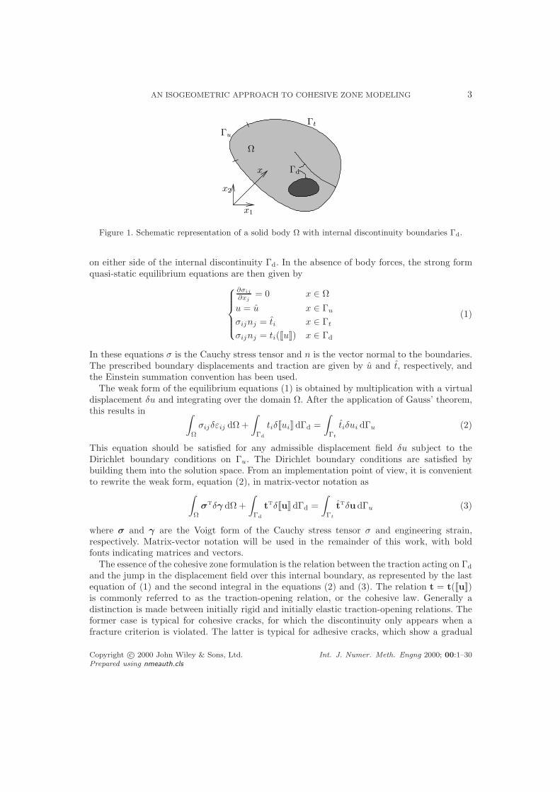
Figure 1. Schematic representation of a solid body Ω with internal discontinuity boundaries Γd.

on either side of the internal discontinuity Γd. In the absence of body forces, the strong formquasi-static equilibrium equations are then given by

∂σij

∂xj= 0 x ∈ Ω

u = u x ∈ Γu

σijnj = ti x ∈ Γt

σijnj = ti(JuK) x ∈ Γd

(1)

In these equations σ is the Cauchy stress tensor and n is the vector normal to the boundaries.The prescribed boundary displacements and traction are given by u and t, respectively, andthe Einstein summation convention has been used.

The weak form of the equilibrium equations (1) is obtained by multiplication with a virtualdisplacement δu and integrating over the domain Ω. After the application of Gauss’ theorem,this results in

∫

Ω

σijδεij dΩ +

∫

Γd

tiδJuiKdΓd =

∫

Γt

tiδui dΓu (2)

This equation should be satisfied for any admissible displacement field δu subject to theDirichlet boundary conditions on Γu. The Dirichlet boundary conditions are satisfied bybuilding them into the solution space. From an implementation point of view, it is convenientto rewrite the weak form, equation (2), in matrix-vector notation as

∫

Ω

σTδγ dΩ +

∫

Γd

tTδJuKdΓd =

∫

Γt

tTδu dΓu (3)

where σ and γ are the Voigt form of the Cauchy stress tensor σ and engineering strain,respectively. Matrix-vector notation will be used in the remainder of this work, with boldfonts indicating matrices and vectors.

The essence of the cohesive zone formulation is the relation between the traction acting on Γd

and the jump in the displacement field over this internal boundary, as represented by the lastequation of (1) and the second integral in the equations (2) and (3). The relation t = t(JuK)is commonly referred to as the traction-opening relation, or the cohesive law. Generally adistinction is made between initially rigid and initially elastic traction-opening relations. Theformer case is typical for cohesive cracks, for which the discontinuity only appears when afracture criterion is violated. The latter is typical for adhesive cracks, which show a gradual



increase in opening before their fracture strength is reached, after which unrecoverable damageaccumulates in the interface. Over the past decades many different traction-opening relationshave been proposed for a wide variety of applications. The two most important parametersused in these models are the fracture strength, which is the maximum traction that can beapplied on an interface, and the fracture toughness, which represents the amount of energydissipated per unit of cracked surface.

In many cases one is interested in studying the evolution of cracks, and their effect on theload bearing capacity of a structure. In those cases, the internal discontinuity boundary Γd

gradually extends through the domain Ω in such a way that Γd(t) ⊆ Γd(t+∆t). The evolutionof the discontinuity is governed by a fracture criterion, which requires the stress state at thecrack tip to be equal to the fracture strength when the crack is propagating. The direction ofpropagation is usually taken perpendicular to that of the maximum principal stress.

Here we apply a staggered solution procedure to model the evolution of the discontinuityboundary, as is also commonly done in partition of unity-based approaches (e.g. [9, 11])and interface elements-based approaches (e.g. [17]). In this staggered approach we solve theequilibrium equations (3) for a fixed internal boundary Γd. If the stresses are such that thefracture criterion inside the domain Ω is violated, we create a new discontinuity. We extend thecrack with an increment that can depend on the employed discretization. A similar approachcan be found in the context of configurational force models for fracture (e.g. [18]).

3. THE ISOGEOMETRIC APPROACH

The fundamental idea of the isogeometric approach is to discretize the cohesive zoneformulation discussed in section 2 using a solution space that: i) exactly represents a broadrange of geometric entities, and ii) allows for discontinuities in the displacement field over theinternal boundaries Γd. We first demonstrate how discontinuities are introduced in B-splinesand non-uniform rational B-splines (NURBS). These basis functions can be considered thefundamental building blocks of isogeometric analysis. We then demonstrate how NURBS canbe used to model pre-defined discontinuities. Next, we introduce T-splines and demonstratetheir superiority to NURBS when used to model propagating discontinuities.

3.1. Discontinuities in B-splines and NURBS

The fundamental building block of isogeometric analysis is the univariate B-spline, e.g. [16,13]. A univariate B-spline is a piecewise polynomial defined over a knot vector Ξ =ξ1, ξ2, . . . , ξn+p+1, with n and p denoting the number and order of basis functions,respectively. The knot values ξi are non-decreasing with increasing knot index i, i.e. ξ1 ≤ξ2 ≤ . . . ≤ ξn+p+1. As a consequence, the knots divide the parametric domain [ξ1, ξn+p+1] ⊂ R

in knot intervals of non-negative length. We refer to the knot intervals of positive length aselements. When several knot values coincide, their multiplicity is indicated by mi, where icorresponds to the index of the knot values. The B-splines used for analysis purposes aregenerally open B-splines, which means that the multiplicity of the first and last knot (m1 andmn+p+1) is equal to p+ 1.



A B-spline of order p is defined as a linear combination of n B-spline basis functions

a(ξ) =

n∑

i=1

Ni,p(ξ)Ai (4)

where Ni,p(ξ) represents a B-spline basis function of order p and Ai is called a control point orvariable. Equation (4) is typically used for the parameterization of curves in two (with Ai ∈ R

2)or three (with Ai ∈ R

3) dimensions. For open B-splines a(ξ1) = A1 and a(ξn+p+1) = An.The B-spline basis is defined recursively, starting with the zeroth order (p = 0) functions

Ni,0(ξ) =

1 ξi ≤ ξ < ξi+1

0 otherwise(5)

from which the higher-order (p = 1, 2, . . .) basis functions follow by the Cox-de Boor recursionformula [19, 20]

Ni,p(ξ) =ξ − ξi

ξi+p − ξiNi,p−1(ξ) +

ξi+p+1 − ξ

ξi+p+1 − ξi+1

Ni+1,p−1(ξ) (6)

Efficient and robust algorithms exist for the evaluation of these non-negative basis functionsand their derivatives, e.g. [21]. B-spline basis functions satisfy the partition of unity property,and B-spline parameterizations possess the variation diminishing property, e.g. [22]. B-splinesare also refineable, which is important in the context of isogeometric analysis, e.g. [23].However, a drawback of B-splines is their inability to exactly represent many objects ofengineering interest, such as conic sections. For this reason NURBS, which are a rationalgeneralization of B-splines, are commonly used. A NURBS is defined as

a(ξ) =

n∑

i=1

Ni,p(ξ)Wi

w(ξ)Ai =

n∑

i=1

Ri,p(ξ)Ai (7)

where w(ξ) =∑n

i=1Ni,p(ξ)Wi is the weighting function. In the special case that Wi = c ∀i,where c may be an arbitrary constant, the NURBS basis reduces to the B-spline basis.

In this contribution, the NURBS (or B-spline) basis is used for both the parameterizationof the geometry and the approximation of the solution space for the displacement field u, thatis

x(ξ) =

n∑

i=1

Ri,p(ξ)Xi (8)

u(ξ) =n∑

i=1

Ri,p(ξ)Ui (9)

We refer to Xi and Ui as the control points and displacement control variables, respectively.In contrast to C0 finite elements, a control point or variable does not generally coincide withan element vertex in the physical space.

The property of NURBS of particular interest for cohesive zone modeling is that they arep−mi times continuously differentiable over a knot i. This allows for the direct discretizationof higher-order differential equations, e.g. [24]. The ability to control inter-element continuityis useful for cohesive zone models, since discontinuities can be inserted arbitrarily by means of



k

L

EA2

P

x

P

EAx

L1 L2

EA1

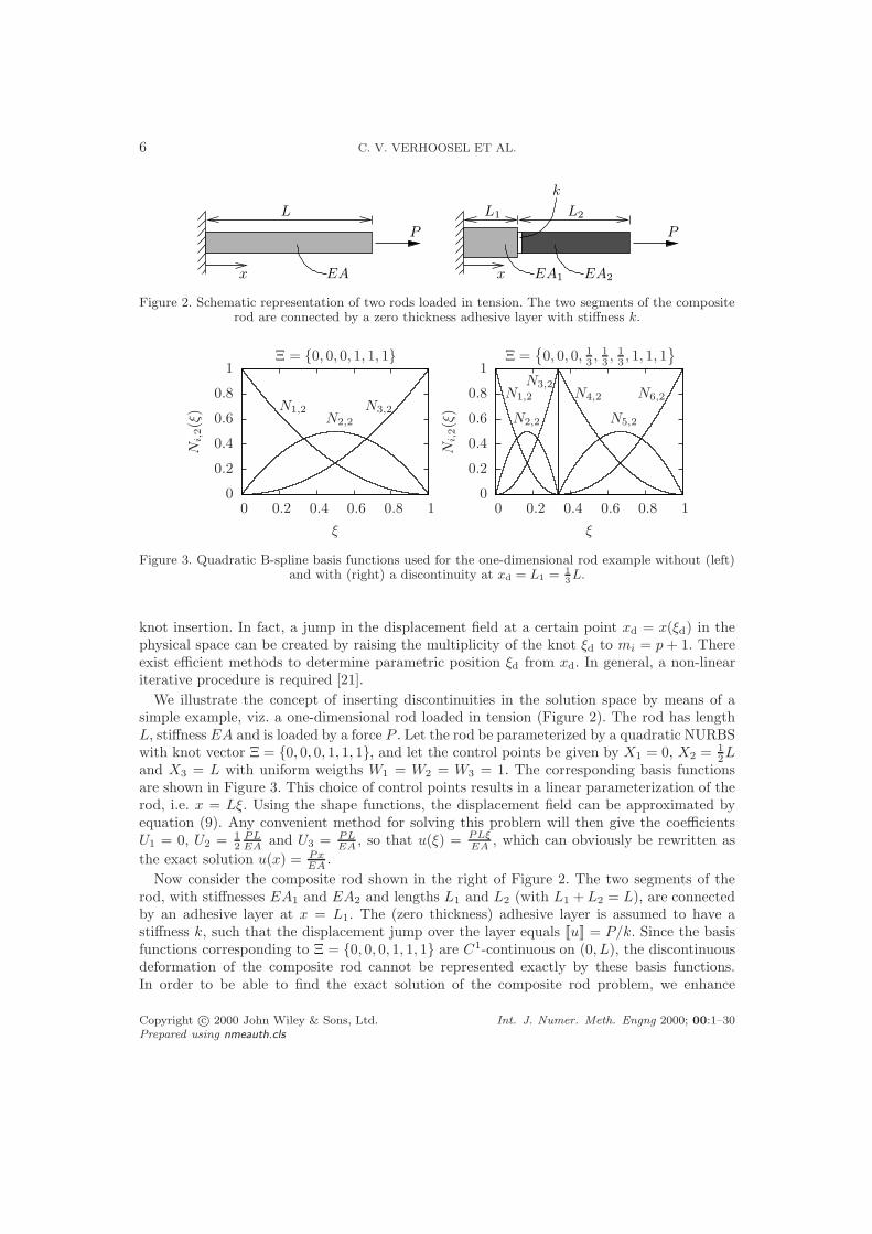
Figure 2. Schematic representation of two rods loaded in tension. The two segments of the compositerod are connected by a zero thickness adhesive layer with stiffness k.

Ξ = 0, 0, 0, 1, 1, 1

N3,2N2,2

N1,2

ξ

Ni,2(ξ

)

10.80.60.40.20

1

0.8

0.6

0.4

0.2

0

Ξ =

0, 0, 0, 13, 1

3, 1

3, 1, 1, 1

N6,2

N5,2

N4,2

N3,2

N2,2

N1,2

ξ

Ni,2(ξ

)

10.80.60.40.20

1

0.8

0.6

0.4

0.2

0

Figure 3. Quadratic B-spline basis functions used for the one-dimensional rod example without (left)and with (right) a discontinuity at xd = L1 = 1

3L.

knot insertion. In fact, a jump in the displacement field at a certain point xd = x(ξd) in thephysical space can be created by raising the multiplicity of the knot ξd to mi = p+ 1. Thereexist efficient methods to determine parametric position ξd from xd. In general, a non-lineariterative procedure is required [21].

We illustrate the concept of inserting discontinuities in the solution space by means of asimple example, viz. a one-dimensional rod loaded in tension (Figure 2). The rod has lengthL, stiffness EA and is loaded by a force P . Let the rod be parameterized by a quadratic NURBSwith knot vector Ξ = 0, 0, 0, 1, 1, 1, and let the control points be given by X1 = 0, X2 = 1

2L

and X3 = L with uniform weigths W1 = W2 = W3 = 1. The corresponding basis functionsare shown in Figure 3. This choice of control points results in a linear parameterization of therod, i.e. x = Lξ. Using the shape functions, the displacement field can be approximated byequation (9). Any convenient method for solving this problem will then give the coefficientsU1 = 0, U2 = 1

2PLEA

and U3 = PLEA

, so that u(ξ) = PLξEA

, which can obviously be rewritten as

the exact solution u(x) = PxEA

.

Now consider the composite rod shown in the right of Figure 2. The two segments of therod, with stiffnesses EA1 and EA2 and lengths L1 and L2 (with L1 +L2 = L), are connectedby an adhesive layer at x = L1. The (zero thickness) adhesive layer is assumed to have astiffness k, such that the displacement jump over the layer equals JuK = P/k. Since the basisfunctions corresponding to Ξ = 0, 0, 0, 1, 1, 1 are C1-continuous on (0, L), the discontinuousdeformation of the composite rod cannot be represented exactly by these basis functions.In order to be able to find the exact solution of the composite rod problem, we enhance



the solution space by allowing for a discontinuity in the displacement field at xd = L1.From the parameterization of the rod we know that this physical position coincides withthe point ξd = L1

Lin the parametric domain. In order to create a discontinuity at xd = L1

we insert a knot with multiplicity p + 1 = 3 at ξ = L1

L, which changes the knot vector to

Ξ =

0, 0, 0, L1

L, L1

L, L1

L, 1, 1, 1

. The corresponding basis functions for the case that L1 = 13L

are shown in Figure 3. When the corresponding control points are taken as X1 = 0, X2 = 12L1,

X3 = L1, X4 = L1, X5 = L1 + 12L2, X6 = L, the original parameterization is preserved.

If we then determine the deformation of the rod using the new basis functions, we find thecoefficients U1 = 0, U2 = 1

2PL1

EA1, U3 = PL1

EA1, U4 = PL1

EA1+ P

k, U5 = PL1

EA1+ P

k+ 1

2PL2

EA2and

U6 = PL1

EA1+ P

k+ PL2

EA2, which is the exact solution to the problem.

3.2. Discretization of a solid with pre-defined discontinuities using NURBS

The isogeometric concept introduced in the previous section can be extended to the multi-dimensional case. In the remainder of this work we restrict ourselves to the two-dimensionalcase. The parameterization of a body Ω ⊂ R

2 can then be obtained by a NURBS surface. Sucha surface can be comprised of one or more NURBS patches. A two-dimensional NURBS patchgives a bivariate parameterization of Ω based on the knot vectors Ξ = ξ1, ξ2, . . . ξn+p+1 andH = η1, η2, . . . ηs+t+1 (such that (ξ, η) ∈ [ξ1, ξn+p+1] ⊗ [η1, ηs+t+1] ⊂ R

2) as

x(ξ, η) =

n∑

i=1

s∑

j=1

Rp,ti,j (ξ, η)Xi,j (10)

in which the bivariate NURBS basis functions are given by

Rp,ti,j (ξ, η) =

Ni,p(ξ)Mj,t(η)Wi,j∑n

ı=1

∑s=1Nı,p(ξ)M,t(η)Wı,

(11)

where Ni,p(ξ) and Mj,t(η) are univariate B-spline basis functions defined over the knot vectorsΞ and H, respectively. From equation (10) it is observed that an arbitrary body Ω can beparametrized by the provision of the nodal control points Xi,j ∈ R

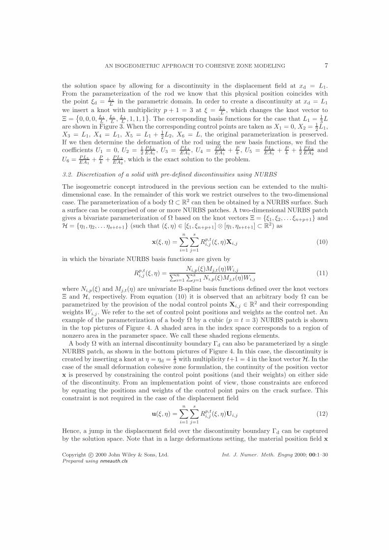
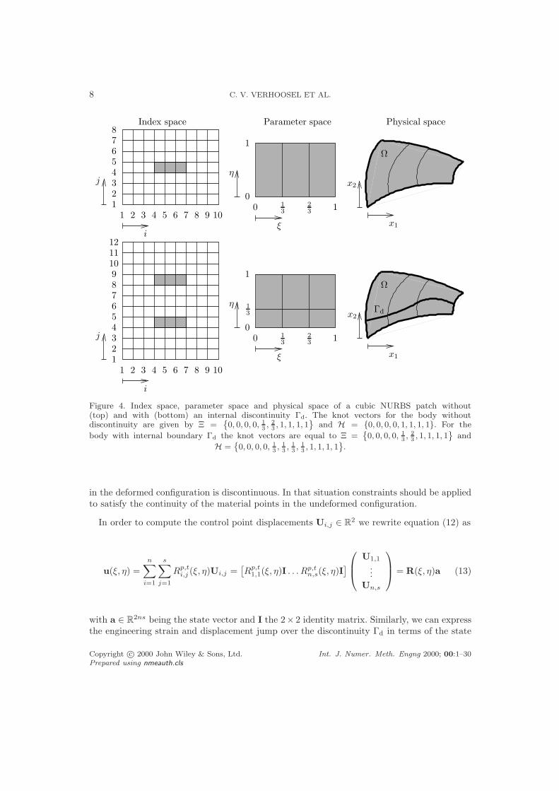
2 and their correspondingweights Wi,j . We refer to the set of control point positions and weights as the control net. Anexample of the parameterization of a body Ω by a cubic (p = t = 3) NURBS patch is shownin the top pictures of Figure 4. A shaded area in the index space corresponds to a region ofnonzero area in the parameter space. We call these shaded regions elements.

A body Ω with an internal discontinuity boundary Γd can also be parameterized by a singleNURBS patch, as shown in the bottom pictures of Figure 4. In this case, the discontinuity iscreated by inserting a knot at η = ηd = 1

3with multiplicity t+1 = 4 in the knot vector H. In the

case of the small deformation cohesive zone formulation, the continuity of the position vectorx is preserved by constraining the control point positions (and their weights) on either sideof the discontinuity. From an implementation point of view, those constraints are enforcedby equating the positions and weights of the control point pairs on the crack surface. Thisconstraint is not required in the case of the displacement field

u(ξ, η) =

n∑

i=1

s∑

j=1

Rp,ti,j (ξ, η)Ui,j (12)

Hence, a jump in the displacement field over the discontinuity boundary Γd can be capturedby the solution space. Note that in a large deformations setting, the material position field x



34

56

78

η

ξ x1

x2

i

j

1

1 2 3 4 5 6 87 9 10

213

23

Index space Physical spaceParameter space

0

0

1

1

Ω

x2

η

ξ

00

1

113

23

i

j

1

1 2 3 4 5 6 7 8 9 10

2

34

56

78

91011

12

x1

Γd

Ω

13

Figure 4. Index space, parameter space and physical space of a cubic NURBS patch without(top) and with (bottom) an internal discontinuity Γd. The knot vectors for the body withoutdiscontinuity are given by Ξ =

˘

0, 0, 0, 0, 1

3, 2

3, 1, 1, 1, 1

¯

and H = 0, 0, 0, 0, 1, 1, 1, 1. For the

body with internal boundary Γd the knot vectors are equal to Ξ =˘

0, 0, 0, 0, 1

3, 2

3, 1, 1, 1, 1

¯

and

H =˘

0, 0, 0, 0, 1

3, 1

3, 1

3, 1

3, 1, 1, 1, 1

¯

.

in the deformed configuration is discontinuous. In that situation constraints should be appliedto satisfy the continuity of the material points in the undeformed configuration.

In order to compute the control point displacements Ui,j ∈ R2 we rewrite equation (12) as

u(ξ, η) =

n∑

i=1

s∑

j=1

Rp,ti,j (ξ, η)Ui,j =

[

Rp,t1,1(ξ, η)I . . . R

p,tn,s(ξ, η)I

]

U1,1

...Un,s

= R(ξ, η)a (13)

with a ∈ R2ns being the state vector and I the 2× 2 identity matrix. Similarly, we can express

the engineering strain and displacement jump over the discontinuity Γd in terms of the state



vector as

γ(ξ, η) =

n∑

i=1

s∑

j=1

Bi,j(ξ, η)Ui,j = B(ξ, η)a (14)

JuK(ξ, η) =

n∑

i=1

s∑

j=1

Mi,j(ξ, η)Ui,j = M(ξ, η)a (15)

in which

Bi,j(ξ, η) =

∂Rp,t

i,j

∂ξ∂ξ∂x

+∂R

p,t

i,j

∂η∂η∂x

0

0∂R

p,t

i,j

∂ξ∂ξ∂y

+∂R

p,t

i,j

∂η∂η∂y

∂Rp,t

i,j

∂ξ∂ξ∂y

+∂R

p,t

i,j

∂η∂η∂y

∂Rp,t

i,j

∂ξ∂ξ∂x

+∂R

p,t

i,j

∂η∂η∂x

(16)

Mi,j(ξ, η) =

limǫ→0

(

Rp,ti,j (ξd + ǫ, η) −Rp,t

i,j (ξd − ǫ, η))

I ξ = ξd

limǫ→0

(

Rp,ti,j (ξ, ηd + ǫ) −Rp,t

i,j (ξ, ηd − ǫ))

I η = ηd

0 otherwise

(17)

with 0 being the 2 × 2 zero matrix. Computation of the matrix in equation (16) requires theevaluation of the Jacobian, which is computed by evaluation of the partial derivatives of theparameterization (10). Substitution of the equations (13), (14) and (15) in the weak form,equation (3), yields the non-linear system of equations

fint(a) = fext (18)

with

fint(a) =

∫

Ω

BTσ dΩ +

∫

Γd

MTt(JuK) dΓd (19)

fext =

∫

Γd

RTt dΓd (20)

The Dirichlet constraints are satisfied by means of constraints on the state vector a,corresponding to the control point displacements Ui,j with nonzero contributions on Γu.A Newton-Raphson solution procedure is then used to solve the non-linear system ofequations (18). The integrals (19) and (20) are evaluated in the parameter domain using aGaussian quadrature, as discussed in Ref. [13]. Improved performance can likely be obtainedby considering more advanced integration rules [25].

As a consequence of the definition of a NURBS patch, a discontinuity inevitably propagatesthroughout a complete patch. In some cases, such as that shown in Figure 4, this allows forthe parameterization of a body with a discontinuity. However, for the more general case ofFigure 1, the body Ω with discontinuities Γd cannot be described by a single NURBS patch.One approach to this problem is to use multiple NURBS patches, tied together with C0

constraints on patch boundaries [13]. In this way, a broad range of bodies with pre-defineddiscontinuities can be discretized.



3.3. Discretization of a solid with propagating discontinuities using T-splines

Combining NURBS patches is generally a cumbersome task. This is particularly so when apropagating discontinuity is considered, since the partitioning of the computational domain byNURBS patches needs to be performed after each nucleation or propagation. For propagatingdiscontinuities it is therefore attractive to use T-splines.

T-splines were introduced by Sederberg et al. [26] and have recently been used foranalysis purposes [27]. Another application of T-splines can be found in [28]. T-splines area generalization of NURBS in the sense that NURBS are a particular class of T-splines.The motivation behind a T-spline can be understood by first considering the localizationof a single basis function in a B-spline or NURBS patch. The basis function Rp,t

i,j may becompletely defined by a set of local knot vectors Ξi,j ⊂ Ξ and Hi,j ⊂ H of length p + 2and t + 2, respectively. In the case that the orders p and t are odd, to which we willrestrict ourselves in this work, the knot vectors associated with the vertex (i, j) in the index

space are Ξi,j =

ξi− p+1

2

, . . . , ξi, . . . , ξi+ p+1

2

and Hi,j =

ηi− t+1

2

, . . . , ηi, . . . , ηi+ t+1

2

with

i ∈

p+3

2, . . . , 2n+p+1

2

and j ∈

t+32, . . . , 2s+t+1

2

. The upper NURBS patch in Figure 4 cantherefore also be represented by means of a T-mesh as shown in the top left picture of Figure 5.Note that in the representation of the T-mesh the outer indices are omitted since the basisfunctions associated with these vertices are zero over the elements (gray areas in Figure 5).If the local knot span of a basis function falls outside the index space, the boundary index isrepeated as many times as necessary. To illustrate this, we present the local knot vectors forthe upper mesh in Figure 5 in Appendix I. Obviously, the number of T-spline basis functionsin this case equals ns, the same as for the NURBS patch in Figure 4.

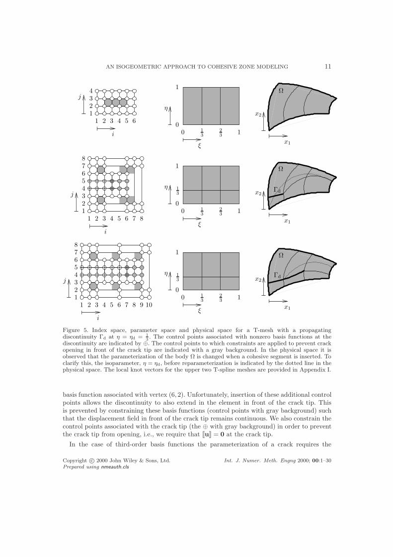
The T-mesh allows for the insertion of discontinuity boundaries locally. In contrast to theNURBS case discussed in the previous section, a discontinuity can be inserted that does notspan the complete width of the index space. If we again consider the example of insertinga crack at ηd = 1

3, we restrict the discontinuity to the leftmost element, by only inserting

horizontal knot lines in the index space until i = 6 (in the middle pictures of Figure 5). Wepresent the local knot vectors for this T-spline mesh in Appendix I. Note that the local knotvectors of the basis functions in the vicinity of the discontinuity are changed, whereas thoseaway from the crack remain unchanged. The crack can propagate by extending the horizontalknot lines in the index space associated with the discontinuity, as shown in the bottom picturesof Figure 5. As can be seen from Figure 5, we extend the knot line throughout the completeT-spline mesh in the parameter and physical space. It is, however, emphasized that only a partof this knot line represents a line of decreased continuity, as indicated by the bold lines in thephysical space. In this work we refer to the shaded areas in the parameter space as elements,which differs from the definition adopted in Ref. [29], where element boundaries are associatedwith lines of decreased continuity.

In Figure 5 the insertion of a C−1 line in the horizontal direction (at ηd = 13) is accompanied

by the insertion of C0 lines (with multiplicity equal to the order) in the vertical direction atξ = 1

3in the center pictures, and additionally at ξ = 2

3in the bottom pictures. These C0

lines are introduced to shield the crack segments from the rest of the domain and from eachother. This is required to satisfy the condition that a crack can only propagate such thatΓd(t) ⊆ Γd(t+ ∆t). Moreover, it allows us to parameterize a crack with the minimum numberof basis functions, denoted by the ⊕ points in Figure 5. Note that additional control pointsare inserted at (i, j) ∈ [5, 6] ⊗ [3, 6] in the center picture to shield the crack from e.g. the



13

i

j

3 4 5 61 21

23

4

i

j

3 4 5 6 7 81 2

12

34

56

78

i

j

1

1 2 3 4 5 6 7 8 9 10

2

34

56

78

η

ξ

00

1

113

23

η

ξ

00

1

113

23

η

ξ

x1

x2

x1

x2

x1

x2

00

1

113

23

13

Ω

Γd

Ω

Ω

Γd

Figure 5. Index space, parameter space and physical space for a T-mesh with a propagatingdiscontinuity Γd at η = ηd = 1

3. The control points associated with nonzero basis functions at the

discontinuity are indicated by ⊕. The control points to which constraints are applied to prevent crackopening in front of the crack tip are indicated with a gray background. In the physical space it isobserved that the parameterization of the body Ω is changed when a cohesive segment is inserted. Toclarify this, the isoparameter, η = ηd, before reparameterization is indicated by the dotted line in thephysical space. The local knot vectors for the upper two T-spline meshes are provided in Appendix I.

basis function associated with vertex (6, 2). Unfortunately, insertion of these additional controlpoints allows the discontinuity to also extend in the element in front of the crack tip. Thisis prevented by constraining these basis functions (control points with gray background) suchthat the displacement field in front of the crack tip remains continuous. We also constrain thecontrol points associated with the crack tip (the ⊕ with gray background) in order to preventthe crack tip from opening, i.e., we require that JuK = 0 at the crack tip.

In the case of third-order basis functions the parameterization of a crack requires the



provision of four relations in the case that the crack path is parameterized by means of apolynomial (the control point weights are all taken equal). These relations are provided byprescribing the position of the crack at both sides of a segment, as well as its normal vectors.A continuous crack path is then obtained by matching the end point of one segment to thestarting point of the next. The differentiability of the crack path is assured by matching thenormal vectors of two adjacent crack segments. Some details on the parameterization of thecrack path are provided in section 4.2.

Upon the extension of a crack, the parameterization of the body Ω is in general changed.In Figure 5 this is visualized by the isoparametric line for η = ηd. This line moves throughthe domain Ω when a cohesive segment is inserted. Before reparameterization of the geometry,the isoparametric line corresponding to η = ηd (dotted lines in the physical space) is notaligned with the discontinuity boundary Γd. Reparameterization of the geometry shifts theisoparameter in order to align it with the discontinuity boundary. For the cohesive zoneformulation this reparameterization is not a fundamental problem, but it requires carefulalgorithmic consideration, see section 4.3.

Since in the case of a T-mesh the approximation of the displacement field can also beexpressed in the form of equation (12), the discretization procedure is exactly the same asfor the NURBS discussed in section 3.2. The fact that the number of basis functions changesupon the insertion of a cohesive segment, requires the recomputation of the converged statevector. Redetermination of the history parameters is also required due to the change inparameterization of the body Ω. These algorithmic aspects are discussed in section 4.4.

4. ALGORITHMIC ASPECTS

In this section some algorithmic aspects that are important for the implementation of theisogeometric framework are discussed. These algorithmic aspects are primarily related to themodeling of propagating discontinuities.

4.1. Direction and instance of propagation

As in the case of partition of unity-based finite element models for discrete fracture, a C0

continuity condition exists at the crack tip. As a result, the stress tensor at the crack tip isgenerally not uniquely defined. The instance of propagation is determined on the basis of thestress tensor in the integration point closest to the crack tip. If the fracture strength of thematerial is exceeded, crack propagation is assumed. Crack nucleation is governed by the samecriterion, evaluated for the stress tensors in all integration points.

As is done in partition of unity-based models, the direction of propagation of a crack isbased on a smoothed stress tensor as suggested in [30]. The smoothed stress is determinedusing the weighting function used in [9]

w =1

(2π)32 l3

exp

(

−‖x − xtip‖

2

2l2

)

(21)

In this weighting function, which should not be confused with the NURBS weighting functionintroduced in section 3.1, l is the smoothing length and xtip is the position of the crack tip.



n2

Nucleation

ξ1ξ2

ηdx1

n1

n2

x2

x3n3

x1

x2

n1

Propagation

ξ1ξ2

ξ3ηd

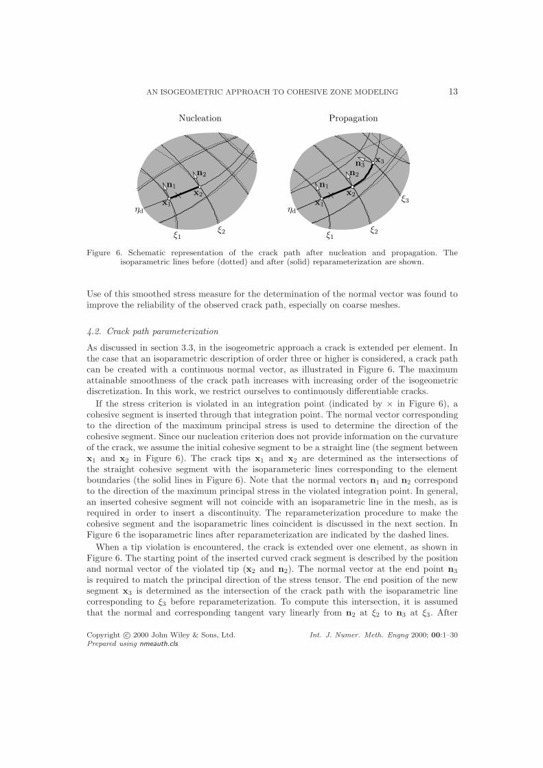
Figure 6. Schematic representation of the crack path after nucleation and propagation. Theisoparametric lines before (dotted) and after (solid) reparameterization are shown.

Use of this smoothed stress measure for the determination of the normal vector was found toimprove the reliability of the observed crack path, especially on coarse meshes.

4.2. Crack path parameterization

As discussed in section 3.3, in the isogeometric approach a crack is extended per element. Inthe case that an isoparametric description of order three or higher is considered, a crack pathcan be created with a continuous normal vector, as illustrated in Figure 6. The maximumattainable smoothness of the crack path increases with increasing order of the isogeometricdiscretization. In this work, we restrict ourselves to continuously differentiable cracks.

If the stress criterion is violated in an integration point (indicated by × in Figure 6), acohesive segment is inserted through that integration point. The normal vector correspondingto the direction of the maximum principal stress is used to determine the direction of thecohesive segment. Since our nucleation criterion does not provide information on the curvatureof the crack, we assume the initial cohesive segment to be a straight line (the segment betweenx1 and x2 in Figure 6). The crack tips x1 and x2 are determined as the intersections ofthe straight cohesive segment with the isoparameteric lines corresponding to the elementboundaries (the solid lines in Figure 6). Note that the normal vectors n1 and n2 correspondto the direction of the maximum principal stress in the violated integration point. In general,an inserted cohesive segment will not coincide with an isoparametric line in the mesh, as isrequired in order to insert a discontinuity. The reparameterization procedure to make thecohesive segment and the isoparametric lines coincident is discussed in the next section. InFigure 6 the isoparametric lines after reparameterization are indicated by the dashed lines.

When a tip violation is encountered, the crack is extended over one element, as shown inFigure 6. The starting point of the inserted curved crack segment is described by the positionand normal vector of the violated tip (x2 and n2). The normal vector at the end point n3

is required to match the principal direction of the stress tensor. The end position of the newsegment x3 is determined as the intersection of the crack path with the isoparametric linecorresponding to ξ3 before reparameterization. To compute this intersection, it is assumedthat the normal and corresponding tangent vary linearly from n2 at ξ2 to n3 at ξ3. After



the insertion of a new cohesive segment, the parameterization of the interior of the domain isaltered in order to align the new cohesive segment with the isoparametric lines of the mesh,as indicated by the difference between the solid and dotted lines in Figure 6.

4.3. Determination of the T-mesh control net

In computer aided design, NURBS and T-splines (among others) are used to parameterizethe geometry. When changes are made to the topology of the mesh, it is desirable topreserve the parameterization. As mentioned in section 3.2, for NURBS, efficient refinementalgorithms exist which preserve parameterization. A T-spline refinement algorithm whichpreserves parameterization was proposed in [31], but appeared to be non-local when appliedin an adaptive analysis environment. The development of efficient local refinement strategiesfor analysis suitable T-splines is an area of active research [32].

The fact that efficient and robust algorithms for T-spline refinement are not yet generallyavailable, however, does not prohibit the type of analysis considered here. This is because therequirements on the preservation of the parameterization when changing the T-mesh topologyare less strict in cohesive zone analyses than in design, where the geometry must be preservedexactly. Of course, it is of crucial importance that the boundaries of the physical domain,including the cracks, remain in the same position. However, the parameterization of the interiorof the domain does not necessarily need to be conserved, as long as the mesh quality remainssatisfactory. In practice this means that the curvatures of the elements should remain bounded.In this respect, the isogeometric approach is not much different from classical finite elements,in which the exact position of the elements is often of minor importance as long as the meshquality is acceptable.

In this contribution we determine the inner control point positions for each T-mesh byrequiring the geometry to minimize the gradients in the parameterization in some sense, whileexactly representing the boundaries and cracks. We solve different problems to determine aninitial mesh and for the control net evolution after the insertion of a cohesive segment. Fornotational convenience we use index notation in this subsection. The physical and parametricposition vectors are given by x ∈ R

2 and ξ ∈ R2, respectively.

• In order to determine the control net for an initial mesh, and its mesh refinements, wesolve an elliptic problem on the parameter domain (here denoted by Ωξ). The problemconsidered here is inspired by the elasticity problem, which minimizes the gradients inthe displacement field. Here we consider a simple problem that is anticipated to minimizethe gradients in the geometry parameterization. The problem is given by

∂∂ξj

(δijψkk + ψij) = 0 ξ ∈ Ωξ

x1 = x1 ξ ∈ Γξx1

x2 = x2 ξ ∈ Γξx2

x = xd ξ ∈ Γξd

(22)

while minimizing the variation in the control weights. In these equations, ψij =12

(

∂xi

∂ξj+

∂xj

∂ξi

)

and Γξx1

and Γξx2

are the boundaries of the parameter domain on which the

position components x1 and x2 are prescribed. The crack position is described by xd onthe internal boundary Γξ

d. Solving the system of equations (22) minimizes the derivatives



of the the physical position vector with respect to the parametric position vector andtherefore prevents the occurrence of steep gradients in the geometry parameterization.To illustrate this, we again consider the uniform one-dimensional rod introduced in

section 3.1. In that case the problem (22) reduces to d2xdξ2

= 0 with boundary conditions

x(0) = 0 and x(1) = L, which results in the linear parameterization x = Lξ.• The update of the control net after the insertion of a cohesive segment is determined

by computing the displacement v of the physical positions with respect to the originalparameterization x. Here we determine the displacement field v by solving a problem onthe physical domain Ω, given by

∂2v1

∂x21

= 0 x ∈ Ω∂2v2

∂x22

= 0 x ∈ Ω

v1 = 0 x ∈ Γv1

v2 = 0 x ∈ Γv2

v = v x ∈ Γd

(23)

such that the new positions of the physical space are given by x = x + v. The changein position required to model the crack, v, is provided by the crack path as described insection 4.2. As for the initial meshes, this system of equations is solved while minimizingthe variation in the control weights. The problem (23) minimizes the gradient of theparameterization in a different way than problem (22). For the numerical simulationsconsidered in section 5, updating the parameterization using problem (23) was foundto yield more robust results than using problem (22). In the case of the composite rod

introduced in section 3.1, the update scheme (23) reduces to d2vdx2 = 0 with boundary

conditions v(0) = v(L) = 0 and v(13L) = v = 0, which results in v = 0 and hence

preserves the parameterization.

The formulations that we used for both cases have proven their suitability for the numericalsimulations considered in section 5, but we emphasize that they are by no means optimal.Improvement of the control net update schemes is a topic of further study.

4.4. State-vector and history values update

As discussed in section 2, a staggered solution scheme is used to trace the evolution of a crackpath. This means that if at some point in the simulation an equilibrium solution u(x) = R(x)ais found in the form of the state vector a, it is possible that this equilibrium state triggers acrack extension and as a consequence results in a change in the T-mesh topology. As a result,the equilibrium state vector a is no longer the discrete form of the equilibrium solution u(x). Infact, the updated T-mesh will consist of more basis functions than the T-mesh on which a wasdetermined. Since the next equilibrium state is determined as an increment to the previouslyconverged state vector, it is necessary to determine the state vector a corresponding to theequilibrium solution u(x) on the updated mesh. We achieve this by minimizing

E =

∫

Ω

∥

∥

∥R(x)a − u(x)

∥

∥

∥

2

dΩ (24)

with R being the T-mesh basis functions on the updated mesh. The updated state vector canthen be determined by solving a linear problem. In the case that the solution space of the old



T-mesh is nested in the new mesh, the functional E in equation (24) will minimize to zero.

Since the parameterization of the body Ω changes upon the insertion of a cohesive segment, itcan also be required to update the history parameters in the integration points. This situationis not encountered here, since history parameters are only considered for the integration pointson the discontinuity boundary, for which the parameterization does not change. In the situationthat history parameters are also used for the interior integration points, their updated valuescan be determined by solving a minimization problem similar to that in equation (24).

5. NUMERICAL SIMULATIONS

We illustrate the isogeometric discretization methods using various typical cohesive zonesimulations. First, we demonstrate the use of a NURBS-based discretization for modeling thedebonding process between a circular fibre and the epoxy it is embedded in. In this examplethe fracture surface is fixed throughout the debonding process, allowing for the use of NURBSand NURBS surfaces. In the second and third numerical simulations we consider propagatingcracks, requiring the use of T-spline discretizations. The second simulation demonstratesthe interaction between an adhesive and a cohesive crack, whereas in the third numericalexperiment multiple cracks appear, including a strongly curved crack. Mesh convergencestudies are presented for all numerical simulations. In those studies it is important to notethat the scaling of the number of degrees of freedom with the number of elements differs fromthat in the case of traditional finite elements.

5.1. Fibre-epoxy debonding experiment

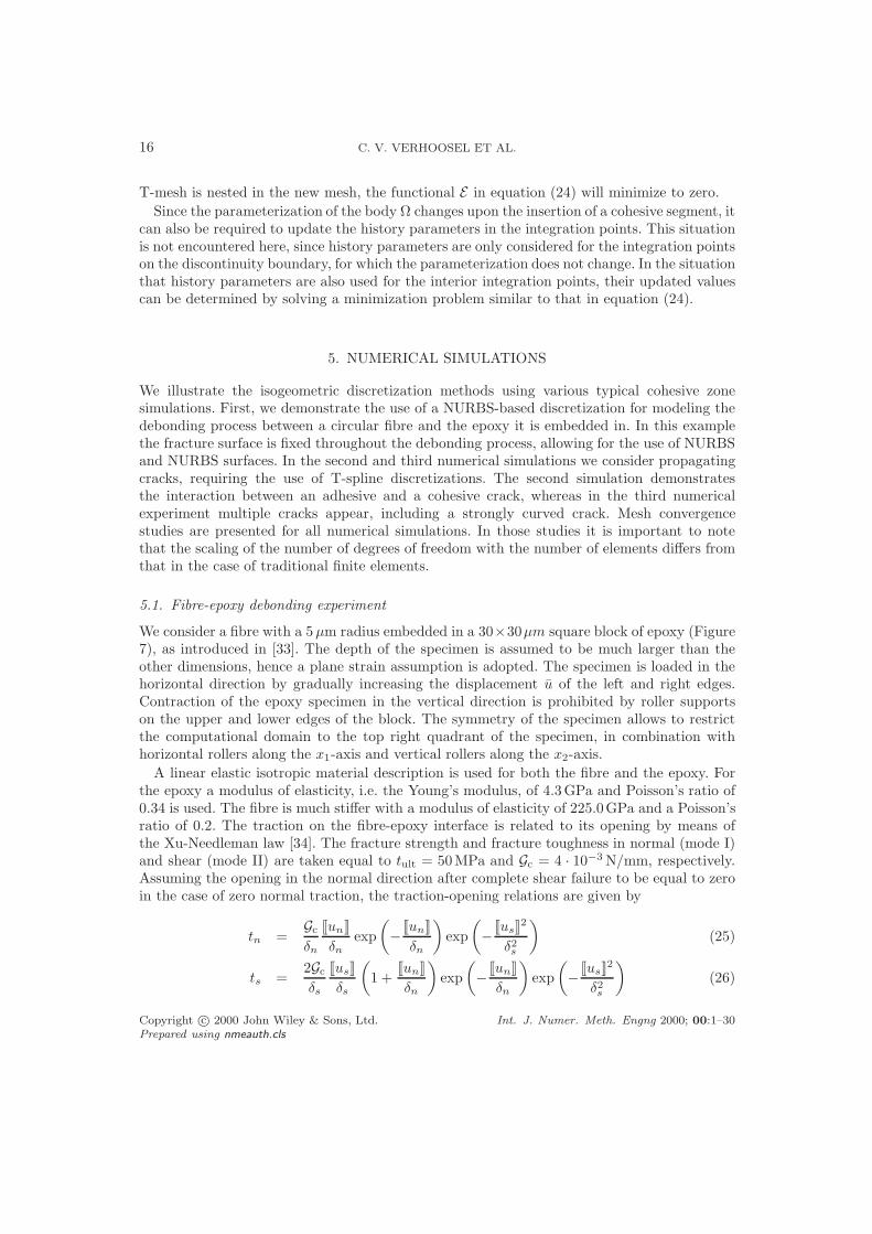
We consider a fibre with a 5µm radius embedded in a 30×30µm square block of epoxy (Figure7), as introduced in [33]. The depth of the specimen is assumed to be much larger than theother dimensions, hence a plane strain assumption is adopted. The specimen is loaded in thehorizontal direction by gradually increasing the displacement u of the left and right edges.Contraction of the epoxy specimen in the vertical direction is prohibited by roller supportson the upper and lower edges of the block. The symmetry of the specimen allows to restrictthe computational domain to the top right quadrant of the specimen, in combination withhorizontal rollers along the x1-axis and vertical rollers along the x2-axis.

A linear elastic isotropic material description is used for both the fibre and the epoxy. Forthe epoxy a modulus of elasticity, i.e. the Young’s modulus, of 4.3GPa and Poisson’s ratio of0.34 is used. The fibre is much stiffer with a modulus of elasticity of 225.0GPa and a Poisson’sratio of 0.2. The traction on the fibre-epoxy interface is related to its opening by means ofthe Xu-Needleman law [34]. The fracture strength and fracture toughness in normal (mode I)and shear (mode II) are taken equal to tult = 50MPa and Gc = 4 · 10−3 N/mm, respectively.Assuming the opening in the normal direction after complete shear failure to be equal to zeroin the case of zero normal traction, the traction-opening relations are given by

tn =Gc

δn

JunK

δnexp

(

−JunK

δn

)

exp

(

−JusK

2

δ2s

)

(25)

ts =2Gc

δs

JusK

δs

(

1 +JunK

δn

)

exp

(

−JunK

δn

)

exp

(

−JusK

2

δ2s

)

(26)



x2

30

u u

30

10

x1

Figure 7. Schematic representation of a fibre with a circular cross section embedded in a square blockof epoxy. All dimensions are in micrometers.

in the case of loading. The parameters δn and δs are the characteristic length parametersthat are related to the fracture strength and fracture toughness by δn = Gc/(tulte) and

δs = Gc/(tult

√

12e) with e = exp (1). The loading condition is checked on the basis of

the history parameter κ and the loading function f =

√

〈JunK〉2

+ β−1JusK2 − κ, with

〈JunK〉 = 12

(|JunK| + JunK) and β = 2.3 the mode-mixity parameter. The history functionf evolves according to the Kuhn-Tucker conditions

f ≤ 0 κ ≥ 0 κf = 0 (27)

In the case of unloading (f < 0), the traction components are related to the crack opening bymeans of the secant stiffnesses. Finally an additional penetration stiffness kp = 1·105 MPa/mmis added in the normal direction in the case of negative crack opening in the normal direction.

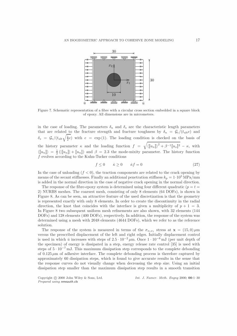
The response of the fibre-epoxy system is determined using four different quadratic (p = t =2) NURBS meshes. The coarsest mesh, consisting of only 8 elements (64 DOFs), is shown inFigure 8. As can be seen, an attractive feature of the used discretization is that the geometryis represented exactly with only 8 elements. In order to create the discontinuity in the radialdirection, the knot that coincides with the interface is given a multiplicity of p + 1 = 3.In Figure 8 two subsequent uniform mesh refinements are also shown, with 32 elements (144DOFs) and 128 elements (400 DOFs), respectively. In addition, the response of the system wasdetermined using a mesh with 2048 elements (4644 DOFs), which we refer to as the referencesolution.

The response of the system is measured in terms of the σx1x1stress at x = (15, 0)µm

versus the prescribed displacement of the left and right edges. Initially displacement controlis used in which u increases with steps of 2.5 · 10−2 µm. Once 1 · 10−8 mJ (per unit depth ofthe specimen) of energy is dissipated in a step, energy release rate control [35] is used withsteps of 5 · 10−7 mJ. This maximum dissipation step corresponds to the complete debondingof 0.125µm of adhesive interface. The complete debonding process is therefore captured byapproximately 60 dissipation steps, which is found to give accurate results in the sense thatthe response curves do not visually change when decreasing the step size. Using an initialdissipation step smaller than the maximum dissipation step results in a smooth transition



Figure 8. NURBS meshes used for the fibre-epoxy simulations. Note that typically the control nodesdo not coincide with the element vertices.

128 elements32 elements8 elements

Reference solution

u [µm]

σx1x1(1

5,0

)[M

Pa]

0.30.250.20.150.10.050

80

70

60

50

40

30

20

10

0

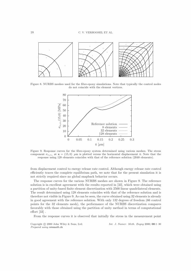
Figure 9. Response curves for the fibre-epoxy system determined using various meshes. The stresscomponent σx1x1

at x = (15, 0) µm is plotted versus the horizontal displacement u. Note that theresponse using 128 elements coincides with that of the reference solution (2048 elements).

from displacement control to energy release rate control. Although energy release rate controlefficiently traces the complete equilibrium path, we note that for the present simulation it isnot strictly required since no global snapback behavior occurs.

The response curves for the various NURBS meshes are shown in Figure 9. The referencesolution is in excellent agreement with the results reported in [33], which were obtained usinga partition of unity-based finite element discretization with 2500 linear quadrilateral elements.The result determined using 128 elements coincides with that of the reference solution and istherefore not visible in Figure 9. As can be seen, the curve obtained using 32 elements is alreadyin good agreement with the reference solution. With only 132 degrees of freedom (66 controlpoints for the 32 elements mesh), the performance of the NURBS discretization comparesfavorably with those obtained using the partition of unity method in terms of computationaleffort [33] .

From the response curves it is observed that initially the stress in the measurement point



σx1x1

[MPa]

30

40

50

60

70

80

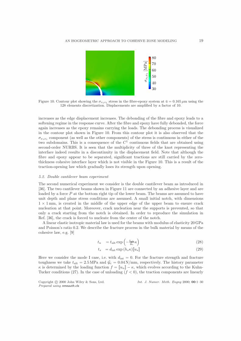
Figure 10. Contour plot showing the σx1x1stress in the fibre-epoxy system at u = 0.165 µm using the

128 elements discretization. Displacements are amplified by a factor of 10.

increases as the edge displacement increases. The debonding of the fibre and epoxy leads to asoftening regime in the response curve. After the fibre and epoxy have fully debonded, the forceagain increases as the epoxy remains carrying the loads. The debonding process is visualizedin the contour plot shown in Figure 10. From this contour plot it is also observed that theσx1x1

component (as well as the other components) of the stress is continuous in either of thetwo subdomains. This is a consequence of the C1 continuous fields that are obtained usingsecond-order NURBS. It is seen that the multiplicity of three of the knot representing theinterface indeed results in a discontinuity in the displacement field. Note that although thefibre and epoxy appear to be separated, significant tractions are still carried by the zero-thickness cohesive interface layer which is not visible in the Figure 10. This is a result of thetraction-opening law which gradually loses its strength upon opening.

5.2. Double cantilever beam experiment

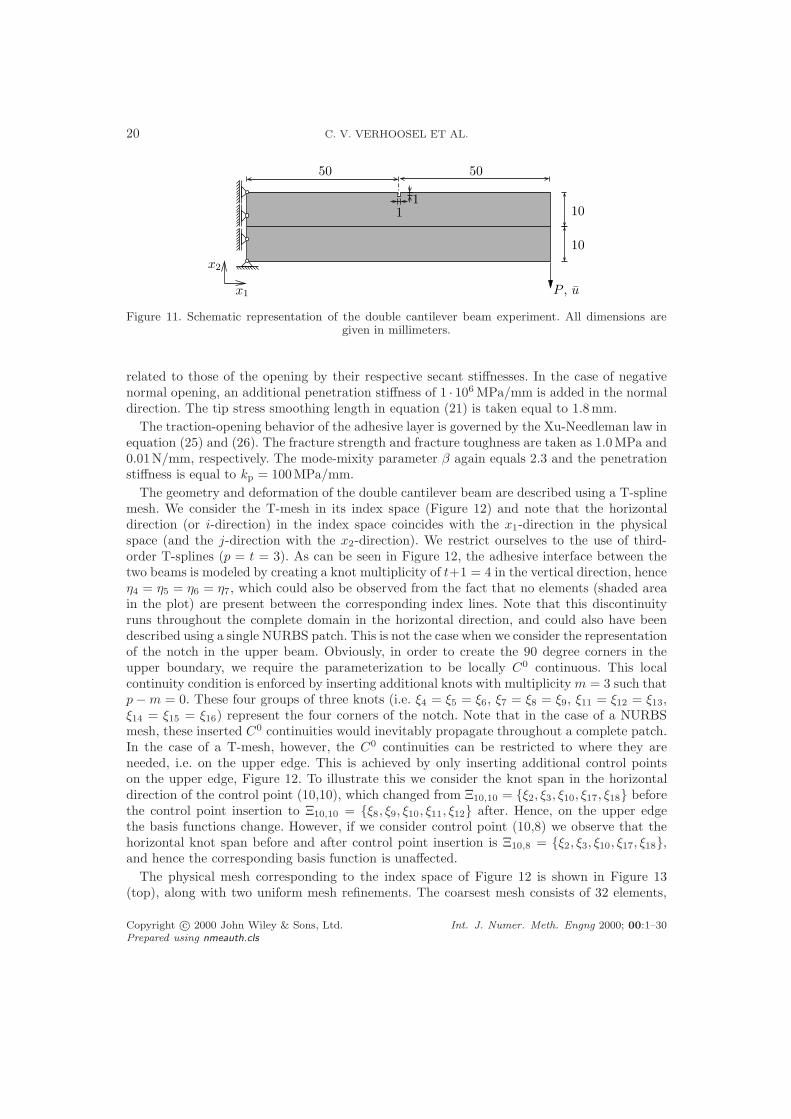
The second numerical experiment we consider is the double cantilever beam as introduced in[36]. The two cantilever beams shown in Figure 11 are connected by an adhesive layer and areloaded by a force P at the bottom right tip of the lower beam. The beams are assumed to haveunit depth and plane stress conditions are assumed. A small initial notch, with dimensions1 × 1 mm, is created in the middle of the upper edge of the upper beam to ensure cracknucleation at that point. Moreover, crack nucleation near the supports is prevented, so thatonly a crack starting from the notch is obtained. In order to reproduce the simulation inRef. [36], the crack is forced to nucleate from the center of the notch.

A linear elastic isotropic material law is used for the beams with modulus of elasticity 20GPaand Poisson’s ratio 0.2. We describe the fracture process in the bulk material by means of thecohesive law, e.g. [9]

tn = tult exp(

− tult

Gcκ)

(28)

ts = dint exp (hsκ)JusK (29)

Here we consider the mode I case, i.e. with dint = 0. For the fracture strength and fracturetoughness we take tult = 2.5MPa and Gc = 0.04N/mm, respectively. The history parameterκ is determined by the loading function f = JunK − κ, which evolves according to the Kuhn-Tucker conditions (27). In the case of unloading (f < 0), the traction components are linearly



50 50

P , u

10

10

x1

x2

11

Figure 11. Schematic representation of the double cantilever beam experiment. All dimensions aregiven in millimeters.

related to those of the opening by their respective secant stiffnesses. In the case of negativenormal opening, an additional penetration stiffness of 1 · 106 MPa/mm is added in the normaldirection. The tip stress smoothing length in equation (21) is taken equal to 1.8mm.

The traction-opening behavior of the adhesive layer is governed by the Xu-Needleman law inequation (25) and (26). The fracture strength and fracture toughness are taken as 1.0MPa and0.01N/mm, respectively. The mode-mixity parameter β again equals 2.3 and the penetrationstiffness is equal to kp = 100MPa/mm.

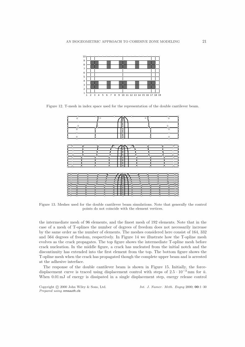
The geometry and deformation of the double cantilever beam are described using a T-splinemesh. We consider the T-mesh in its index space (Figure 12) and note that the horizontaldirection (or i-direction) in the index space coincides with the x1-direction in the physicalspace (and the j-direction with the x2-direction). We restrict ourselves to the use of third-order T-splines (p = t = 3). As can be seen in Figure 12, the adhesive interface between thetwo beams is modeled by creating a knot multiplicity of t+1 = 4 in the vertical direction, henceη4 = η5 = η6 = η7, which could also be observed from the fact that no elements (shaded areain the plot) are present between the corresponding index lines. Note that this discontinuityruns throughout the complete domain in the horizontal direction, and could also have beendescribed using a single NURBS patch. This is not the case when we consider the representationof the notch in the upper beam. Obviously, in order to create the 90 degree corners in theupper boundary, we require the parameterization to be locally C0 continuous. This localcontinuity condition is enforced by inserting additional knots with multiplicity m = 3 such thatp−m = 0. These four groups of three knots (i.e. ξ4 = ξ5 = ξ6, ξ7 = ξ8 = ξ9, ξ11 = ξ12 = ξ13,ξ14 = ξ15 = ξ16) represent the four corners of the notch. Note that in the case of a NURBSmesh, these inserted C0 continuities would inevitably propagate throughout a complete patch.In the case of a T-mesh, however, the C0 continuities can be restricted to where they areneeded, i.e. on the upper edge. This is achieved by only inserting additional control pointson the upper edge, Figure 12. To illustrate this we consider the knot span in the horizontaldirection of the control point (10,10), which changed from Ξ10,10 = ξ2, ξ3, ξ10, ξ17, ξ18 beforethe control point insertion to Ξ10,10 = ξ8, ξ9, ξ10, ξ11, ξ12 after. Hence, on the upper edgethe basis functions change. However, if we consider control point (10,8) we observe that thehorizontal knot span before and after control point insertion is Ξ10,8 = ξ2, ξ3, ξ10, ξ17, ξ18,and hence the corresponding basis function is unaffected.

The physical mesh corresponding to the index space of Figure 12 is shown in Figure 13(top), along with two uniform mesh refinements. The coarsest mesh consists of 32 elements,



1 2 3 4 5 6 7 8 9 10 11 12 13 14 15 16 17 18 191

2

3

4

5

6

7

8

9

10

Figure 12. T-mesh in index space used for the representation of the double cantilever beam.

Figure 13. Meshes used for the double cantilever beam simulations. Note that generally the controlpoints do not coincide with the element vertices.

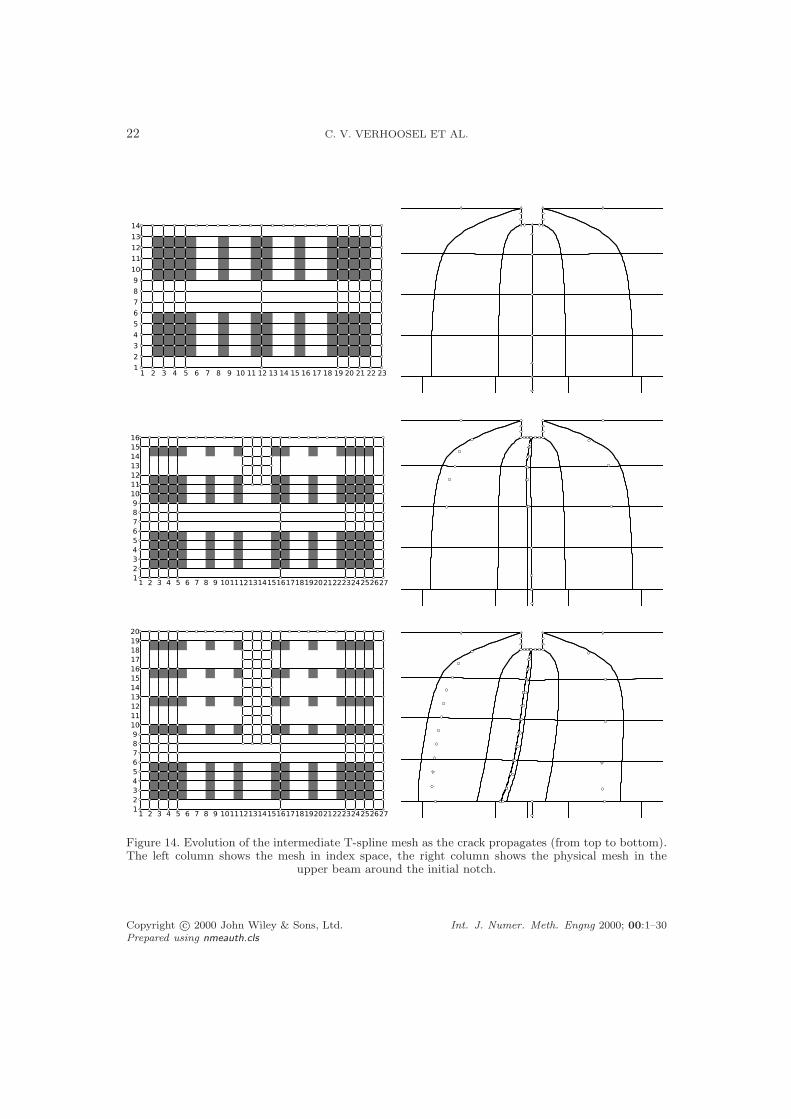
the intermediate mesh of 96 elements, and the finest mesh of 192 elements. Note that in thecase of a mesh of T-splines the number of degrees of freedom does not necessarily increaseby the same order as the number of elements. The meshes considered here consist of 164, 332and 564 degrees of freedom, respectively. In Figure 14 we illustrate how the T-spline meshevolves as the crack propagates. The top figure shows the intermediate T-spline mesh beforecrack nucleation. In the middle figure, a crack has nucleated from the initial notch and thediscontinuity has extended into the first element from the top. The bottom figure shows theT-spline mesh when the crack has propagated though the complete upper beam and is arrestedat the adhesive interface.

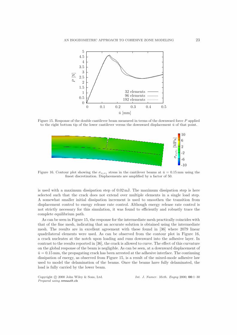
The response of the double cantilever beam is shown in Figure 15. Initially, the force-displacement curve is traced using displacement control with steps of 2.5 · 10−3 mm for u.When 0.01mJ of energy is dissipated in a single displacement step, energy release control



1 2 3 4 5 6 7 8 9 10 11 12 13 14 15 16 17 18 19 20 21 22 231

2

3

4

5

6

7

8

9

10

11

12

13

14

1 2 3 4 5 6 7 8 9 10111213141516171819202122232425262712345678910111213141516

1 2 3 4 5 6 7 8 9 1011121314151617181920212223242526271234567891011121314151617181920

Figure 14. Evolution of the intermediate T-spline mesh as the crack propagates (from top to bottom).The left column shows the mesh in index space, the right column shows the physical mesh in the

upper beam around the initial notch.




u [mm]

P[N

]

0.50.40.30.20.10

5

4.5

4

3.5

3

2.5

2

1.5

1

0.5

0

Figure 15. Response of the double cantilever beam measured in terms of the downward force P appliedto the right bottom tip of the lower cantilever versus the downward displacement u of that point.

σx1x1

[MPa]

-10

-6

-2

2

6

10

Figure 16. Contour plot showing the σx1x1stress in the cantilever beams at u = 0.15 mm using the

finest discretization. Displacements are amplified by a factor of 50.

is used with a maximum dissipation step of 0.02mJ. The maximum dissipation step is hereselected such that the crack does not extend over multiple elements in a single load step.A somewhat smaller initial dissipation increment is used to smoothen the transition fromdisplacement control to energy release rate control. Although energy release rate control isnot strictly necessary for this simulation, it was found to efficiently and robustly trace thecomplete equilibrium path.

As can be seen in Figure 15, the response for the intermediate mesh practically coincides withthat of the fine mesh, indicating that an accurate solution is obtained using the intermediatemesh. The results are in excellent agreement with these found in [36] where 2079 linearquadrilateral elements were used. As can be observed from the contour plot in Figure 16,a crack nucleates at the notch upon loading and runs downward into the adhesive layer. Incontrast to the results reported in [36], the crack is allowed to curve. The effect of this curvatureon the global response of the beam is negligible. As can be seen, at a downward displacement ofu = 0.15 mm, the propagating crack has been arrested at the adhesive interface. The continuingdissipation of energy, as observed from Figure 15, is a result of the mixed-mode adhesive lawused to model the delamination of the beams. Once the beams have fully delaminated, theload is fully carried by the lower beam.



x2

180 180

80

111P

1011P

2020

x1

20

20

20

5

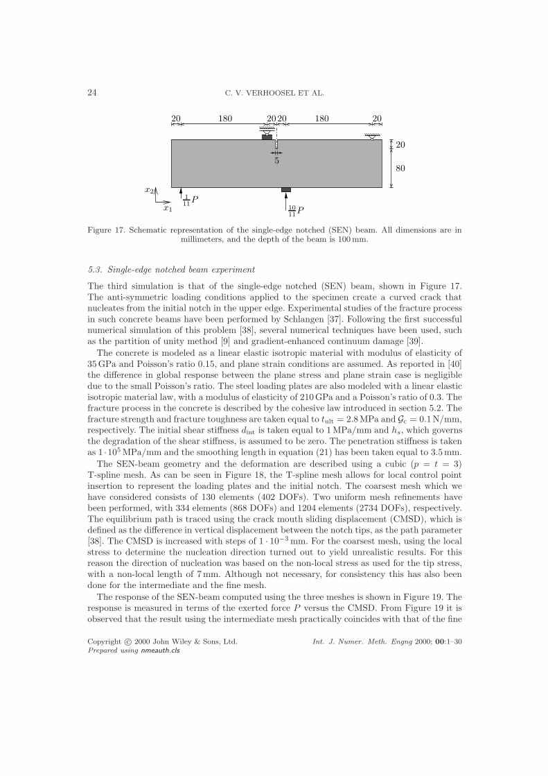
Figure 17. Schematic representation of the single-edge notched (SEN) beam. All dimensions are inmillimeters, and the depth of the beam is 100 mm.

5.3. Single-edge notched beam experiment

The third simulation is that of the single-edge notched (SEN) beam, shown in Figure 17.The anti-symmetric loading conditions applied to the specimen create a curved crack thatnucleates from the initial notch in the upper edge. Experimental studies of the fracture processin such concrete beams have been performed by Schlangen [37]. Following the first successfulnumerical simulation of this problem [38], several numerical techniques have been used, suchas the partition of unity method [9] and gradient-enhanced continuum damage [39].

The concrete is modeled as a linear elastic isotropic material with modulus of elasticity of35GPa and Poisson’s ratio 0.15, and plane strain conditions are assumed. As reported in [40]the difference in global response between the plane stress and plane strain case is negligibledue to the small Poisson’s ratio. The steel loading plates are also modeled with a linear elasticisotropic material law, with a modulus of elasticity of 210GPa and a Poisson’s ratio of 0.3. Thefracture process in the concrete is described by the cohesive law introduced in section 5.2. Thefracture strength and fracture toughness are taken equal to tult = 2.8MPa and Gc = 0.1N/mm,respectively. The initial shear stiffness dint is taken equal to 1 MPa/mm and hs, which governsthe degradation of the shear stiffness, is assumed to be zero. The penetration stiffness is takenas 1 ·105 MPa/mm and the smoothing length in equation (21) has been taken equal to 3.5mm.

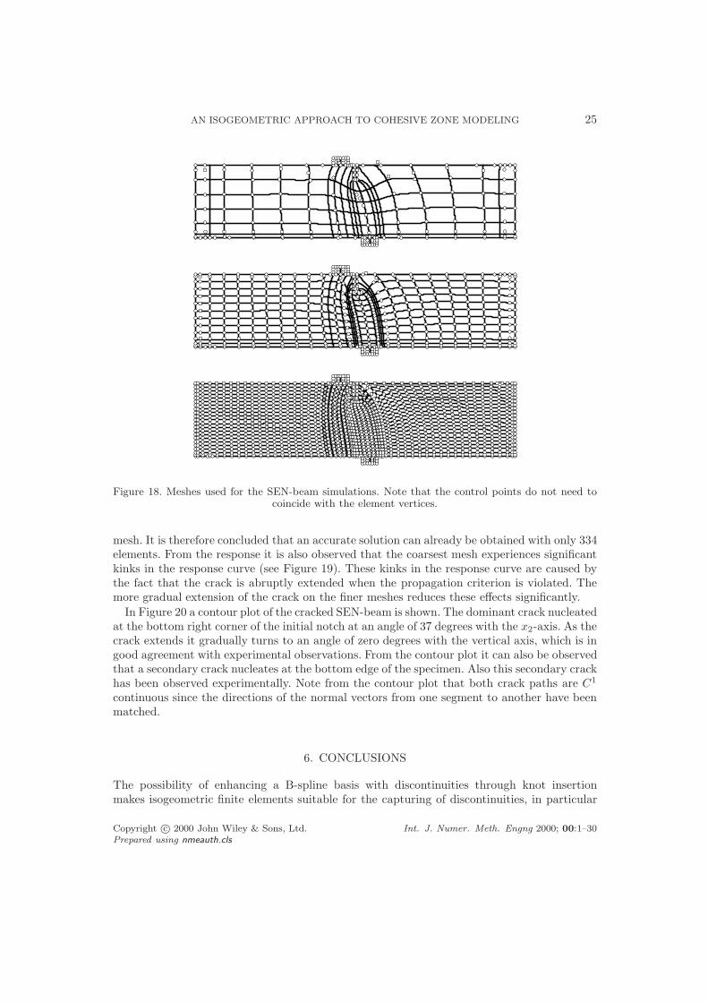
The SEN-beam geometry and the deformation are described using a cubic (p = t = 3)T-spline mesh. As can be seen in Figure 18, the T-spline mesh allows for local control pointinsertion to represent the loading plates and the initial notch. The coarsest mesh which wehave considered consists of 130 elements (402 DOFs). Two uniform mesh refinements havebeen performed, with 334 elements (868 DOFs) and 1204 elements (2734 DOFs), respectively.The equilibrium path is traced using the crack mouth sliding displacement (CMSD), which isdefined as the difference in vertical displacement between the notch tips, as the path parameter[38]. The CMSD is increased with steps of 1 · 10−3 mm. For the coarsest mesh, using the localstress to determine the nucleation direction turned out to yield unrealistic results. For thisreason the direction of nucleation was based on the non-local stress as used for the tip stress,with a non-local length of 7mm. Although not necessary, for consistency this has also beendone for the intermediate and the fine mesh.

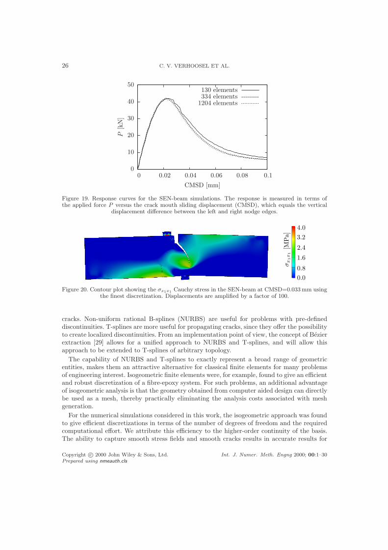
The response of the SEN-beam computed using the three meshes is shown in Figure 19. Theresponse is measured in terms of the exerted force P versus the CMSD. From Figure 19 it isobserved that the result using the intermediate mesh practically coincides with that of the fine



Figure 18. Meshes used for the SEN-beam simulations. Note that the control points do not need tocoincide with the element vertices.

mesh. It is therefore concluded that an accurate solution can already be obtained with only 334elements. From the response it is also observed that the coarsest mesh experiences significantkinks in the response curve (see Figure 19). These kinks in the response curve are caused bythe fact that the crack is abruptly extended when the propagation criterion is violated. Themore gradual extension of the crack on the finer meshes reduces these effects significantly.

In Figure 20 a contour plot of the cracked SEN-beam is shown. The dominant crack nucleatedat the bottom right corner of the initial notch at an angle of 37 degrees with the x2-axis. As thecrack extends it gradually turns to an angle of zero degrees with the vertical axis, which is ingood agreement with experimental observations. From the contour plot it can also be observedthat a secondary crack nucleates at the bottom edge of the specimen. Also this secondary crackhas been observed experimentally. Note from the contour plot that both crack paths are C1

continuous since the directions of the normal vectors from one segment to another have beenmatched.

6. CONCLUSIONS

The possibility of enhancing a B-spline basis with discontinuities through knot insertionmakes isogeometric finite elements suitable for the capturing of discontinuities, in particular




CMSD [mm]

P[k

N]

0.10.080.060.040.020

50

40

30

20

10

0

Figure 19. Response curves for the SEN-beam simulations. The response is measured in terms ofthe applied force P versus the crack mouth sliding displacement (CMSD), which equals the vertical

displacement difference between the left and right nodge edges.

σx1x1

[MPa]

0.0

4.0

0.8

1.6

2.4

3.2

Figure 20. Contour plot showing the σx1x1Cauchy stress in the SEN-beam at CMSD=0.033 mm using

the finest discretization. Displacements are amplified by a factor of 100.

cracks. Non-uniform rational B-splines (NURBS) are useful for problems with pre-defineddiscontinuities. T-splines are more useful for propagating cracks, since they offer the possibilityto create localized discontinuities. From an implementation point of view, the concept of Bezierextraction [29] allows for a unified approach to NURBS and T-splines, and will allow thisapproach to be extended to T-splines of arbitrary topology.

The capability of NURBS and T-splines to exactly represent a broad range of geometricentities, makes them an attractive alternative for classical finite elements for many problemsof engineering interest. Isogeometric finite elements were, for example, found to give an efficientand robust discretization of a fibre-epoxy system. For such problems, an additional advantageof isogeometric analysis is that the geometry obtained from computer aided design can directlybe used as a mesh, thereby practically eliminating the analysis costs associated with meshgeneration.

For the numerical simulations considered in this work, the isogeometric approach was foundto give efficient discretizations in terms of the number of degrees of freedom and the requiredcomputational effort. We attribute this efficiency to the higher-order continuity of the basis.The ability to capture smooth stress fields and smooth cracks results in accurate results for



relatively coarse meshes. The advantages of higher-order continuity are expected to be moreprofound in the case of slender structures, making isogeometric finite elements suitable formodeling cracks in, for instance, shells.

The isogeometric approach to cohesive zone formulations is anticipated to be applicable to abroad range of problems with propagating discontinuity boundaries. The configurational forcemodels for brittle fracture [18] are examples of such problems. In this contribution we haveenhanced the solution space with discontinuities by means of knot insertion, but isogeometricanalysis can also be used in combination with the partition of unity method. We finally notethat the concept of Bezier extraction not only unifies the treatment of NURBS and T-splines,but potentially also reduces the complexity of the implementation. Easing the implementationof the presented method is desirable, particularly when three-dimensional models are to beconsidered.

ACKNOWLEDGEMENTS

T. J.R. Hughes and M. A. Scott were partially supported by ONR Contract N00014-08-0992, T. J.R.Hughes was also partially supported by NSF Grant 0700204, and M.A. Scott was also partiallysupported by an ICES CAM Graduate Fellowship.

APPENDIX

I. T-spline knot vectors: An illustration

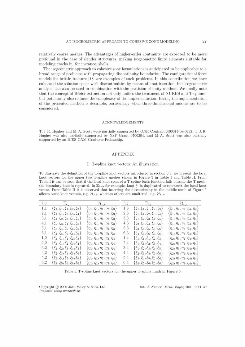
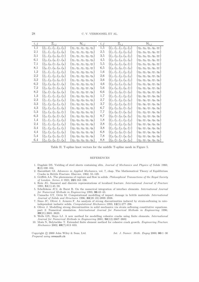
To illustrate the definition of the T-spline knot vectors introduced in section 3.3, we present the localknot vectors for the upper two T-spline meshes shown in Figure 5 in Table I and Table II. FromTable I it can be seen that if the local knot span of a T-spline basis function falls outside the T-mesh,the boundary knot is repeated. In Ξ2,4, for example, knot ξ1 is duplicated to construct the local knotvector. From Table II it is observed that inserting the discontinuity in the middle mesh of Figure 5affects some knot vectors, e.g. H2,3, whereas others are unaltered, e.g. H8,2.

i, j Ξi,j Hi,j

1,1 ξ1, ξ1, ξ1, ξ2, ξ3 η1, η1, η1, η2, η32,1 ξ1, ξ1, ξ2, ξ3, ξ4 η1, η1, η1, η2, η33,1 ξ1, ξ2, ξ3, ξ4, ξ5 η1, η1, η1, η2, η34,1 ξ2, ξ3, ξ4, ξ5, ξ6 η1, η1, η1, η2, η35,1 ξ3, ξ4, ξ5, ξ6, ξ6 η1, η1, η1, η2, η36,1 ξ4, ξ5, ξ6, ξ6, ξ6 η1, η1, η1, η2, η31,2 ξ1, ξ1, ξ1, ξ2, ξ3 η1, η1, η2, η3, η42,2 ξ1, ξ1, ξ2, ξ3, ξ4 η1, η1, η2, η3, η43,2 ξ1, ξ2, ξ3, ξ4, ξ5 η1, η1, η2, η3, η44,2 ξ2, ξ3, ξ4, ξ5, ξ6 η1, η1, η2, η3, η45,2 ξ3, ξ4, ξ5, ξ6, ξ6 η1, η1, η2, η3, η46,2 ξ4, ξ5, ξ6, ξ6, ξ6 η1, η1, η2, η3, η4

i, j Ξi,j Hi,j

1,3 ξ1, ξ1, ξ1, ξ2, ξ3 η1, η2, η3, η4, η42,3 ξ1, ξ1, ξ2, ξ3, ξ4 η1, η2, η3, η4, η43,3 ξ1, ξ2, ξ3, ξ4, ξ5 η1, η2, η3, η4, η44,3 ξ2, ξ3, ξ4, ξ5, ξ6 η1, η2, η3, η4, η45,3 ξ3, ξ4, ξ5, ξ6, ξ6 η1, η2, η3, η4, η46,3 ξ4, ξ5, ξ6, ξ6, ξ6 η1, η2, η3, η4, η41,4 ξ1, ξ1, ξ1, ξ2, ξ3 η2, η3, η4, η4, η42,4 ξ1, ξ1, ξ2, ξ3, ξ4 η2, η3, η4, η4, η43,4 ξ1, ξ2, ξ3, ξ4, ξ5 η2, η3, η4, η4, η44,4 ξ2, ξ3, ξ4, ξ5, ξ6 η2, η3, η4, η4, η45,4 ξ3, ξ4, ξ5, ξ6, ξ6 η2, η3, η4, η4, η46,4 ξ4, ξ5, ξ6, ξ6, ξ6 η2, η3, η4, η4, η4

Table I. T-spline knot vectors for the upper T-spline mesh in Figure 5.



i, j Ξi,j Hi,j

1,1 ξ1, ξ1, ξ1, ξ2, ξ3 η1, η1, η1, η2, η32,1 ξ1, ξ1, ξ2, ξ3, ξ6 η1, η1, η1, η2, η33,1 ξ1, ξ2, ξ3, ξ6, ξ7 η1, η1, η1, η2, η36,1 ξ2, ξ3, ξ6, ξ7, ξ8 η1, η1, η1, η2, η37,1 ξ3, ξ6, ξ7, ξ8, ξ8 η1, η1, η1, η2, η78,1 ξ6, ξ7, ξ8, ξ8, ξ8 η1, η1, η1, η2, η71,2 ξ1, ξ1, ξ1, ξ2, ξ3 η1, η1, η2, η3, η42,2 ξ1, ξ1, ξ2, ξ3, ξ6 η1, η1, η2, η3, η43,2 ξ1, ξ2, ξ3, ξ6, ξ7 η1, η1, η2, η3, η46,2 ξ2, ξ3, ξ6, ξ7, ξ8 η1, η1, η2, η3, η47,2 ξ3, ξ6, ξ7, ξ8, ξ8 η1, η1, η2, η7, η88,2 ξ6, ξ7, ξ8, ξ8, ξ8 η1, η1, η2, η7, η81,3 ξ1, ξ1, ξ1, ξ2, ξ3 η1, η2, η3, η4, η52,3 ξ1, ξ1, ξ2, ξ3, ξ4 η1, η2, η3, η4, η53,3 ξ1, ξ2, ξ3, ξ4, ξ5 η1, η2, η3, η4, η54,3 ξ2, ξ3, ξ4, ξ5, ξ6 η1, η2, η3, η4, η55,3 ξ3, ξ4, ξ5, ξ6, ξ7 η1, η2, η3, η4, η56,3 ξ4, ξ5, ξ6, ξ7, ξ8 η1, η2, η3, η4, η51,4 ξ1, ξ1, ξ1, ξ2, ξ3 η2, η3, η4, η5, η62,4 ξ1, ξ1, ξ2, ξ3, ξ4 η2, η3, η4, η5, η63,4 ξ1, ξ2, ξ3, ξ4, ξ5 η2, η3, η4, η5, η64,4 ξ2, ξ3, ξ4, ξ5, ξ6 η2, η3, η4, η5, η65,4 ξ3, ξ4, ξ5, ξ6, ξ7 η2, η3, η4, η5, η66,4 ξ4, ξ5, ξ6, ξ7, ξ8 η2, η3, η4, η5, η6

i, j Ξi,j Hi,j

1,5 ξ1, ξ1, ξ1, ξ2, ξ3 η3, η4, η5, η6, η72,5 ξ1, ξ1, ξ2, ξ3, ξ4 η3, η4, η5, η6, η73,5 ξ1, ξ2, ξ3, ξ4, ξ5 η3, η4, η5, η6, η74,5 ξ2, ξ3, ξ4, ξ5, ξ6 η3, η4, η5, η6, η75,5 ξ3, ξ4, ξ5, ξ6, ξ7 η3, η4, η5, η6, η76,5 ξ4, ξ5, ξ6, ξ7, ξ8 η3, η4, η5, η6, η71,6 ξ1, ξ1, ξ1, ξ2, ξ3 η4, η5, η6, η7, η82,6 ξ1, ξ1, ξ2, ξ3, ξ4 η4, η5, η6, η7, η83,6 ξ1, ξ2, ξ3, ξ4, ξ5 η4, η5, η6, η7, η84,6 ξ2, ξ3, ξ4, ξ5, ξ6 η4, η5, η6, η7, η85,6 ξ3, ξ4, ξ5, ξ6, ξ7 η4, η5, η6, η7, η86,6 ξ4, ξ5, ξ6, ξ7, ξ8 η4, η5, η6, η7, η81,7 ξ1, ξ1, ξ1, ξ2, ξ3 η5, η6, η7, η8, η82,7 ξ1, ξ1, ξ2, ξ3, ξ6 η5, η6, η7, η8, η83,7 ξ1, ξ2, ξ3, ξ6, ξ7 η5, η6, η7, η8, η86,7 ξ2, ξ3, ξ6, ξ7, ξ8 η5, η6, η7, η8, η87,7 ξ3, ξ6, ξ7, ξ8, ξ8 η1, η2, η7, η8, η88,7 ξ6, ξ7, ξ8, ξ8, ξ8 η1, η2, η7, η8, η81,8 ξ1, ξ1, ξ1, ξ2, ξ3 η6, η7, η8, η8, η82,8 ξ1, ξ1, ξ2, ξ3, ξ6 η6, η7, η8, η8, η83,8 ξ1, ξ2, ξ3, ξ6, ξ7 η6, η7, η8, η8, η86,8 ξ2, ξ3, ξ6, ξ7, ξ8 η6, η7, η8, η8, η87,8 ξ3, ξ6, ξ7, ξ8, ξ8 η2, η7, η8, η8, η88,8 ξ6, ξ7, ξ8, ξ8, ξ8 η2, η7, η8, η8, η8

Table II. T-spline knot vectors for the middle T-spline mesh in Figure 5.

REFERENCES

1. Dugdale DS. Yielding of steel sheets containing slits. Journal of Mechanics and Physics of Solids 1960;8(2):100–104.

2. Barenblatt GI. Advances in Applied Mechanics, vol. 7, chap. The Mathematical Theory of EquilibriumCracks in Brittle Fracture. Elsevier, 1962; 55–129.

3. Griffith AA. The phenomena of rupture and flow in solids. Philosophical Transactions of the Royal Societyof London. Series A 1921; 221:163–198.

4. Rots JG. Smeared and discrete representations of localized fracture. International Journal of Fracture1991; 51(1):45–59.

5. Schellekens JCJ, de Borst R. On the numerical integration of interface elements. International Journalfor Numerical Methods in Engineering 1993; 36:43–43.

6. Camacho GT, Ortiz M. Computational modelling of impact damage in brittle materials. InternationalJournal of Solids and Structures 1996; 33(20–22):2899–2938.

7. Simo JC, Oliver J, Armero F. An analysis of strong discontinuities induced by strain-softening in rate-independent inelastic solids. Computational Mechanics 1993; 12(5):277–296.

8. Oliver J. Modelling strong discontinuities in solid mechanics via strain softening constitutive equations.part 2: Numerical simulation. International Journal for Numerical Methods in Engineering 1996;39(21):3601–3623.

9. Wells GN, Sluys LJ. A new method for modelling cohesive cracks using finite elements. InternationalJournal for Numerical Methods in Engineering 2001; 50(12):2667–2682.

10. Moes N, Belytschko T. Extended finite element method for cohesive crack growth. Engineering FractureMechanics 2002; 69(7):813–833.



11. Remmers JJC, de Borst R, Needleman A. A cohesive segments method for the simulation of crack growth.Computational mechanics 2003; 31(1-2):69–77.

12. Hughes TJR, Cottrell JA, Bazilevs Y. Isogeometric analysis: CAD, finite elements, NURBS, exact geometryand mesh refinement. Computer Methods in Applied Mechanics and Engineering 2005; 194(39–41):4135–4195.

13. Cottrell JA, Hughes TJR, Bazilevs Y. Isogeometric Analysis: Toward Integration of CAD and FEA. Wiley:Chichester, 2009.

14. Wall WA, Frenzel MA, Cyron C. Isogeometric structural shape optimization. Computer Methods in AppliedMechanics and Engineering 2008; 197(33-40):2976–2988.

15. Elguedj T, Bazilevs Y, Calo VM, Hughes TJR. B-bar and F-bar projection methods for nearlyincompressible linear and non-linear elasticity and plasticity using higher-order NURBS elements.Computer Methods in Applied Mechanics and Engineering 2008; 197(33-40):2732–2762.

16. Rogers DF. An Introduction to NURBS. Academic Press: San Diego, 2001.17. Tijssens MGA, Sluys LJ, van der Giessen E. Simulation of fracture of cementitious composites with explicit

modeling of microstructural features. Engineering Fracture Mechanics 2001; 68(11):1245–1263.18. Miehe C, Gurses E. A robust algorithm for configurational-force-driven brittle crack propagation with R-

adaptive mesh alignment. International Journal for Numerical Methods in Engineering 2007; 72(2):127–155.

19. Cox MG. The numerical evaluation of B-splines. IMA Journal of Applied Mathematics 1972; 10(2).20. de Boor C. On calculating with B-splines. Journal of Approximation Theory 1972; 6(1):50–62.21. Piegl L, Tiller W. The NURBS Book. second edn., Springer-Verlag: Berlin, 1997.22. Farin G. Curves and Surfaces for CAGD. Academic Press, Inc., 1993.23. Cottrell JA, Hughes TJR, Reali A. Studies of refinement and continuity in isogeometric structural analysis.

Computer Methods in Applied Mechanics and Engineering 2007; 196(41–44):4160–4183.24. Gomez H, Calo VM, Bazilevs Y, Hughes TJR. Isogeometric analysis of the Cahn-Hilliard phase-field model.

Computer Methods in Applied Mechanics and Engineering 2008; 197(49-50):4333–4352.25. Hughes TJR, Reali A, Sangalli G. Efficient quadrature for NURBS-based isogeometric analysis. Computer

Methods in Applied Mechanics and Engineering 2010; 199(5-8):301–313.26. Sederberg TW, Zheng J, Bakenov A, Nasri A. T-splines and T-NURCCs. ACM Transactions on Graphics

2003; 22(3):477–484.27. Bazilevs Y, Calo VM, Cottrell JA, Evans JA, Hughes TJR, Lipton S, Scott MA, Sederberg TW.

Isogeometric analysis using T-splines. Computer Methods in Applied Mechanics and Engineering 2010;199(5–8):229–263.

28. Benson DJ, Bazilevs Y, De Luycker E, Hsu MC, Scott MA, Hughes TJR, Belytschko T. A generalizedfinite element formulation for arbitrary basis functions: from isogeometric analysis to XFEM. InternationalJournal for Numerical Methods in Engineering 2010; DOI: 10.1002/nme.2864.

29. Borden MJ, Scott MA, Evans JA, Hughes TJR. Isogeometric finite element data structures basedon Bezier extraction. International Journal for Numerical Methods in Engineering 2010; DOI:10.1002/nme.2968.

30. Jirasek M. Comparative study on finite elements with embedded discontinuities. Computer Methods inApplied Mechanics and Engineering 2000; 188(1-3):307–330.

31. Sederberg TW, Cardon DL, Finnigan GT, North NS, Zheng J, Lyche T. T-spline simplification and localrefinement. ACM Transactions on Graphics 2004; 23(3):276–283.

32. Scott MA, Borden MJ, Hughes TJR. Bezier-based isogeometric methods: Formulation. Proceedings of the10th US National Congress on Computatinal Mechanics, 2009.

33. Remmers JJC. Discontinuities in materials and structures. PhD Thesis, Delft University of Technology2006.

34. Xu XP, Needleman A. Void nucleation by inclusion debonding in a crystal matrix. Modelling andSimulation in Materials Science and Engineering 1993; 1(2):111–132.

35. Verhoosel CV, Remmers JJC, Gutierrez MA. A dissipation-based arc-length method for robust simulationof brittle and ductile failure. International Journal for Numerical Methods in Engineering 2009;77(9):1290–1321.

36. de Borst R, Remmers JJC, Needleman A, Abellan MA. Discrete vs smeared crack models for concretefracture: bridging the gap. Mechanics of Cohesive-frictional Materials 2004; 28(7-8):583–607.

37. Schlangen E. Experimental and numerical analysis of fracture processes in concrete. PhD Thesis, DelftUniversity of Technology 1993.

38. de Borst R. Computation of post-bifurcation and post-failure behavior of strain-softening solids. Computers& Structures 1987; 25(2):211–224.

39. Geers MGD, de Borst R, Peerlings RHJ. Damage and crack modeling in single-edge and double-edgenotched concrete beams. Engineering Fracture Mechanics 2000; 65(2-3):247–261.

40. Wells GN. Discontinuous modelling of strain localisation and failure. PhD Thesis, Delft University of



Technology 2001.


An isogeometric approach to cohesive zone modelingeprints.whiterose.ac.uk/96215/8/WRRO_96215.pdf ·...

Documents

Transcript of An isogeometric approach to cohesive zone modelingeprints.whiterose.ac.uk/96215/8/WRRO_96215.pdf ·...