An investigation on image denoising technique using pixel ...

Innovative Systems Design and Engineering www.iiste.org

ISSN 2222-1727 (Paper) ISSN 2222-2871 (Online)

Vol 2, No 4, 2011

233

An investigation on image denoising technique

using pixel-component-analysis

S.Kathiravan

Department of Electronics and Communication Engineering,

Kalaignar Karunanidhi Institute of Technology, Coimbatore, India

Tel: 0091-7708914377 Email: [email protected]

N. Guhan Raja



Tel: 0091-9944288113 Email: guhanraja16 @gmail.com

R. Arun Kumar



Tel: 0091-9095811465 Email: arunkumar.soft18 @gmail.com

Abstract:

This paper authenticates a proficient image denoising scheme with the analysis local pixel coherence. In the

dominion of a study about noise and pixel elements in image processing, the influence of the Gaussian effect on

image contrast plays a key role. It is found in particular that pixel variations may be vast in some cases which

potentially tend to develop irregularities in the image.

Scope and preamble:

A customary way to remove noise from image data is to employ spatial filters. Owing to these basic methods, there

exists certain disadvantage also. The process by which manifestation of digital image is recovered from noisy

signals is identified to be Denoising (M. Elad & M. Aharon, 2006). The prior objective is to enhance the appearance

of any image by using the new concept in Denoising. Here some basic existing methods are given below.

1. Existing methods:

1.1Spatial filtering:

1.1.1 Non linear filters:

In this filter noise is removed without any attempt made to identify it. Spatial filters employ a low pass filtering on

group of pixels with the assumption that noise occupies higher region of frequency region of frequency spectrum.

Normally spatial filters remove noise upto an extent, but in case of blurring images, inturn make the edges in picture

invisible sometimes.

1.1.2 Linear filter:

This filter reduces Gaussian noise in the sense of mean square error. Linear filters do tend to blur sharp edges,

destroy lines and other fine image details and perform poorly in the presence of the signal dependent noise.

mailto:[email protected]





Vol 2, No 4, 2011

234

In case of Weiner filtering method, it requires the information about the spectra of noise and the original signal. This

method implements spatial smoothing and its model complexity control correspond to choosing the values of

window size (A.K.Jain, 1989) . To overcome the weakness of wiener filtering, other advanced methods were found.

2. Transform domain filtering:

2.1 Spatial frequency filtering:

This refers to use of low pass filters using FFT. In frequency smoothing methods, the removal of noise is achieved

by designing a frequency domain filter and adopting a cut-off frequency when the noise components are

decorrelated from the useful signal in frequency domain.

These methods are bit time consuming and depend on the cut-off frequency and filter functions. They also may

produce artificial frequency in processed image.

2.2 Wavelet domain filtering:

Here assumption of filtered image that is more visually displeasing than the original noisy signal, even though the

filtering operation noisy signal, even though the filtering operation successfully reduces the noise (S. Mallat, 1998).

It involves sparsity property of wavelet transform and it maps white noise in the signal domain to white noise in

transform domain. Thus despite the facts that signal energy become more concentrated into fewer coefficients in the

transform domain, enables separation of signal from noise.

Thus, denoising is often a necessary and the first step to be taken before the images data is analyzed. It is necessary

to apply an efficient denoising technique to compensate for such data corruption.

Data adaptive thresholds (H. Zhang, 2000) were introduced to achieve optimum value of threshold. Later efforts

found that substantial improvements in perceptual quality could be obtained by translation invariant methods based

on thresholding of an undecimated Wavelet Transform (R. Coifman & D. Donoho, 1995). These thresholding

techniques were applied to the non-orthogonal wavelet coefficients to reduce artifacts.

3. Proposed method:

Whenever an image is processed or applied for segmentation, there exist a few irregularities in the alignment and

parameters of the image. This is mainly due to the noise caused by white Gaussian effect (J. Portilla & V. Strela,

2003). Here a concept of denoising is introduced in order to recover the affected image. The process of recovery of

digital image which is affected by noise is called denoising.

Accordingly denoising is done in 2 stages by principal component analysis (D.D. Muresan & T.W.

Parks, 2003) using local pixel coherence. Now the problem is how to estimate the noise by extracting the

underlying pixel. Applying such procedures, even by using various filters to each pixel component the whole image

can be denoised. Some of the existing low level image processing procedure is smoothing filter, frequency domain

method, wavelet transform, and non local mean based method.

Consider wavelet transform, its very effective in noise removal. It decomposes the input image into

multiple segments. Each segment has individual pixel components with different frequency components. At each

segments operations like thresholding and stastical modeling (Marteen Jansen, 2000) can be performed to suppress

noise. Noisy components are eliminated through demonstrating each segment of an image with fixed wavelet basis.

But in the case of natural images, there is a rich amount of pixel elements which cannot be represented using fixed

wavelet basis. Therefore wavelet transform methods can introduce many visual antifacts in the denoising output.

To overcome the problem non local mean approaches were developed. The major idea behind this method

is to show a relationship the similar image pixels. For instance, consider an image is divided multiple segments.

Each segment is labeled by using pixel value. Then mean of each pixel are taken to find out the average value. By

determining the average value, which are having pixel value closer to average value are combined together for

image analysis.



Vol 2, No 4, 2011

235

4. SYSTEM:

Each pixel is estimated as the weighted average of all the pixels in the image, and the weights are determined by the

similarity between the pixels. This technique can also be correlated with patch matching and sparse 3D transform.

A sparse 3D transform is then applied to 3D images and noise was concealed by applying wiener filtering in the

transformed domain.

4.1 LPC-PCA DENOISING ALGORITHM:

An image pixel is described by 2 quantities the spatial locations (K. Dabov & A. Foi, 2007) and its

intensity, while the image local structure is represented as a part of neighbouring pixels at different intensity levels.

Since most of the isolated information of an image is conveyed by its edges.

Therefore irregularities at the edges are highly desired in image denoising. In this concept pixel and its nearest

neighbours as a vector variable and perform noise reduction on the vector instead of single pixel.

Consider the modeling of LPC-PCA based denoising.

The L×L training block

The pixel to be denoised

The K×K variable block

Fig.1 Illustration of the modeling of LPG-PCA based denoising. Referring to the figure 1, set of K*K window centered on it, and it is denoted by

a= [a1. . . . .am]T

m=k2 ,the vector containing all the components within the window. Since the above image is noise

corrupted, it is denoted by av=a+v.

Where, a = noise vector

Here av=[a1

v. . . . amv]

T , V=[v1. . . . vm]

T .To estimate a and a

v,identify vector variables

(ie.noiseless and noisy vector).

By using PCA, analysis of training samples of av, its neighbouring vector is carried out for PCA

transformation.The simplest way is to take the pixels in each possible K*K block within the L*L training block as

the samples of noisy variables av, its neighbouring vector is carried out for PCA transformation. The simplest way is

to take the pixel in each possible K*K block within the L*L training block as the samples of noisy variables av. In

this way there are totally (L-K+1)2 training samples for each component of a and av. However there can be different

blocks from the given central K*K block in the L*L training window so that taking all the K*K blocks as the

training samples of av will lead to inaccurate estimation of the covariance matrix of av, which subsequently leads to

inaccurate estimation of PCA transformation matrix and finally results in noise residual. Therefore selecting and

coherence the training samples that are similar to the central K*K block is necessary for applying PCA transform in

denoising.

5. LPC (Local pixel coherence):

Alignment of training samples which are evaluated from fig 1, the central blocks K*K and L*L is used for

coherence. Thus different coherence methods which are used here is blocking, correlation-based matching. K-mean

clustering depends upon certain criteria.

Concert of denoising algorithms is considered using quantitative performance measures such as Peak signal-to-noise

ratio (PSNR), signal-to-noise ratio (SNR) as well as in terms of visual quality of the images. Many of the current



Vol 2, No 4, 2011

236

techniques assume the noise model to be Gaussian. In this assumption, image appearance is varied due to nature and

sources of noise.

An ideal denoising procedure requires a prior knowledge of the noise, whereas a practical procedure may not have

the required information about the variance of the noise or the noise model. Thus, most of the algorithms assume

known variance of the noise and the noise model to compare the performance with different algorithms. Gaussian

Noise (P. Moulin & J. Liu, 1999) with different variance values is added in the natural images to test the

performance of the algorithm.

6. Denoising of color images:

There are mainly two reasons for the noise residual. First, because of the strong noise in the original dataset X t,

the covariance matrix Xxt is much noise corrupted, which leads to estimation bias of the PCA transformation matrix

and hence deteriorates the denoising performance; second, the strong noise in the original dataset will also lead to

LPC errors, which consequently results in estimation bias of the covariance matrix Xx (or Xxt). Performance of

denoising algorithms is measured using quantitative performance measures (Z. Wang & A.C. Bovik, 2004) such as

peak signal-to-noise ratio (PSNR), signal-to-noise ratio (SNR) as well as in terms of visual quality of the images.

Many of the recent techniques assume the noise model to be Gaussian. In actual fact, this statement may not always

seize factual due to the varied nature and sources of noise. Therefore, it is necessary to further process the denoising

output for a better noise reduction. Since the noise has been much removed in the first round of LPC-PCA

denoising, the LPC accuracy and the estimation of Xx (or X xt ) can be much improved with the denoised image.

Thus we can implement the LPC-PCA denoising procedure for the second round to enhance the denoising results.

On the base of denoising concept we have evaluated and compared the different methods by using two measures:

PSNR and SSIM. PSNR can measure the intensity difference between two images, it is recognized that it may fail to

depict the visual perception of the image. Alternatively, how to evaluate the visual quality of an image is a very

difficult problem and it is currently an active research topic. The SSIM index proposed in one of the most commonly

used measures for image visual quality assessment (A. Pizurica & W. Philips, 2006). Compared with PSNR, SSIM

can better reflect the structure similarity between the target image and the reference image.

Based on the experimental results obtained below shows the PSNR values corresponding to different values of

sigma.

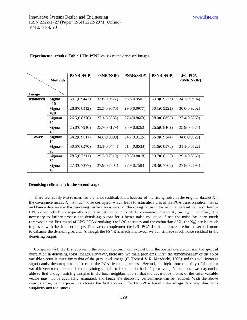
Table.1 lists the PSNR and SSIM measures of the first stage and second stage denoising outputs on the test image

set. We can see that the second stage can improve 0.1–1.5 dB the PSNR values for different images under different

noise level (s is from 10 to 40). Although for some images the second stage will not improve much the PSNR

measures, the SSIM measures, which can better reflect the image visual quality, can be much improved.



Vol 2, No 4, 2011

237



Vol 2, No 4, 2011

238

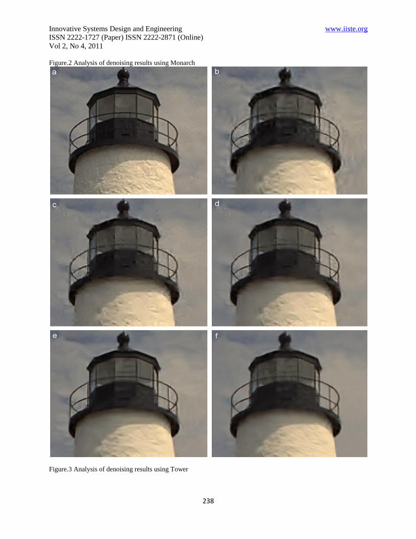
Figure.2 Analysis of denoising results using Monarch

Figure.3 Analysis of denoising results using Tower



Vol 2, No 4, 2011

239

Experimental results: Table.1 The PSNR values of the denoised images

Methods

Image

PSNR(SSIP) PSNR(SSIP) PSNR(SSIP) PSNR(SSIP) LPC-PCA

PSNR(SSIP)

Monarch Sigma

=10

33.1(0.9442) 33.6(0.9527) 33.5(0.9501) 33.9(0.9577) 34.2(0.9594)

Sigma

=20

28.8(0.8912) 29.5(0.9076) 29.6(0.9077) 30.1(0.9222) 30.0(0.9202)

Sigma=

30

26.5(0.8370) 27.1(0.8583) 27.4(0.8663) 28.0(0.8850) 27.4(0.8769)

Sigma =

40

25.0(0.7916) 25.7(0.8179) 25.9(0.8260) 26.6(0.8462) 25.9(0.8378)

Tower Sigma=

10

34.2(0.9017) 34.6(0.9099) 34.7(0.9115) 35.0(0.9144) 34.8(0.9123)

Sigma=

20

30.5(0.8270) 31.1(0.8444) 31.4(0.8533) 31.6(0.8576) 31.1(0.8522)

Sigma=

30

28.5(0.7711) 29.2(0.7919) 29.3(0.8018) 29.7(0.8135) 29.1(0.8069)

Sigma=

40

27.3(0.7277) 27.9(0.7505) 27.9(0.7583) 28.3(0.7760) 27.8(0.7695)

Denoising refinement in the second stage:

There are mainly two reasons for the noise residual. First, because of the strong noise in the original dataset X t,

the covariance matrix Xxt is much noise corrupted, which leads to estimation bias of the PCA transformation matrix

and hence deteriorates the denoising performance; second, the strong noise in the original dataset will also lead to

LPC errors, which consequently results in estimation bias of the covariance matrix Xx (or Xxt). Therefore, it is

necessary to further process the denoising output for a better noise reduction. Since the noise has been much

removed in the first round of LPC-PCA denoising, the LPC accuracy and the estimation of Xx (or Xxt) can be much

improved with the denoised image. Thus we can implement the LPC-PCA denoising procedure for the second round

to enhance the denoising results. Although the PSNR is much improved, we can still see much noise residual in the

denoising output.

Compared with the first approach, the second approach can exploit both the spatial correlation and the spectral

correlation in denoising color images. However, there are two main problems. First, the dimensionality of the color

variable vector is three times that of the gray level image (C. Tomasi & R. Manduchi, 1998) and this will increase

significantly the computational cost in the PCA denoising process. Second, the high dimensionality of the color

variable vector requires much more training samples to be found in the LPC processing. Nonetheless, we may not be

able to find enough training samples in the local neighborhood so that the covariance matrix of the color variable

vector may not be accurately estimated, and hence the denoising performance can be reduced. With the above

consideration, in this paper we choose the first approach for LPC-PCA based color image denoising due to its

simplicity and robustness.



Vol 2, No 4, 2011

240

Results on analysis:

Values of sigma

Figure.4 Illustration of PSNR values

CONCLUSION:

Analysis of the processed image data is one of the hot topics in imaging field where Error probability plays vital

role. This paper has evaluated the global denoising performance with the real distribution of image processing in a

viewing format. The results are particularly encouraging especially because of the comparison with the other

techniques like wavelet transform and frequency domain methods. This is a simplistic method for improving the

standards of an image by pixel alignment with all possible screening performances as a classification feature.Thus

finally the concept of denoising investigates common errors that occurs during image processing and effectively

replaces fine structures of the given input image.



Vol 2, No 4, 2011

241

References:

M. Aharon, M. Elad, A.M. Bruckstein, The K-SVD: an algorithm for designing of over complete dictionaries for

sparse representation, IEEE Transaction on Signal Processing 54 (11) (2006) 4311–4322.

A.K.Jain, Fundamentals of digital image processing. Prentice-Hall, 1989

S. Mallat, Wavelet Tour of Signal Processing, Academic Press, New York, 1998.

H. Zhang, Aria Nosratinia, and R. O. Wells, Jr., “Image denoising via wavelet-domain spatially adaptive

FIR Wiener filtering”, in IEEE Proc. Int. Conf. Acoust., Speech, Signal Processing, Istanbul, Turkey, June

2000.

R. Coifman and D. Donoho, "Translation invariant de-noising," in Lecture Notes in Statistics: Wavelets

And Statistics, vol. New York: Springer-Verlag, pp. 125--150, 1995

J. Portilla, V. Strela, M.J. Wainwright, E.P. Simoncelli, Image denoising using scale mixtures of Gaussians in the

wavelet domain, IEEE Transaction on Image Processing 12 (11) (2003) 1338–1351.

D.D. Muresan, T.W. Parks, Adaptive principal components and image denoising, in: Proceedings of the 2003

International Conference on Image Processing, 14–17 September, vol. 1, 2003, pp. I101–I104.

Marteen Jansen, Ph. D. Thesis in “Wavelet thresholding and noise reduction” 2000.

Z. Wang, A.C. Bovik, H.R. Sheikh, E.P. Simoncelli, Image quality assessment: from error visibility to structural

similarity, IEEE Transaction on Image Processing 13 (4) (2004)

A.Pizurica, W. Philips, Estimating the probability of the presence of a signal of interest in multiresolution single-

and multiband image denoising, IEEE Transaction on Image Processing 15 (3) (2006) 654–665.

K. Dabov, A. Foi, V. Katkovnik, K. Egiazarian, Image denoising by sparse 3D transform-domain collaborative

filtering, IEEE Transaction on Image Processing 16 (8) (2007) 2080–2095

P. Moulin and J. Liu, “Analysis of multiresolution image denoising schemes using generalized Gaussian

And complexity priors”, IEEE Infor. Theory, Vol. 45, No 3, Apr. 1999, pp. 909-919.

C. Tomasi, R. Manduchi, Bilateral filtering for gray and colour images, in: Proceedings of the 1998 IEEE

International Conference on Computer Vision, Bombay, India, 1998, pp. 839–846

This academic article was published by The International Institute for Science,

Technology and Education (IISTE). The IISTE is a pioneer in the Open Access

Publishing service based in the U.S. and Europe. The aim of the institute is

Accelerating Global Knowledge Sharing.

More information about the publisher can be found in the IISTE’s homepage:

http://www.iiste.org

The IISTE is currently hosting more than 30 peer-reviewed academic journals and

collaborating with academic institutions around the world. Prospective authors of

IISTE journals can find the submission instruction on the following page:

http://www.iiste.org/Journals/

The IISTE editorial team promises to the review and publish all the qualified

submissions in a fast manner. All the journals articles are available online to the

readers all over the world without financial, legal, or technical barriers other than

those inseparable from gaining access to the internet itself. Printed version of the

journals is also available upon request of readers and authors.

IISTE Knowledge Sharing Partners

EBSCO, Index Copernicus, Ulrich's Periodicals Directory, JournalTOCS, PKP Open

Archives Harvester, Bielefeld Academic Search Engine, Elektronische

Zeitschriftenbibliothek EZB, Open J-Gate, OCLC WorldCat, Universe Digtial

Library , NewJour, Google Scholar

http://www.iiste.org/

http://www.iiste.org/Journals/

An investigation on image denoising technique using pixel ...

Documents

Transcript of An investigation on image denoising technique using pixel ...