KTH Engineering Sciences

An Investigation of the Iron-Ore Wheel Damages

using Vehicle Dynamics Simulation

Saeed Hossein Nia Licentiate Thesis

Stockholm, Sweden

2014

I

Academic thesis with permission by KTH Royal Institute of Technology, Stockholm, to be submitted for public examination for the degree of Licentiate of Engineering in Vehicle and Maritime Engineering.

TRTA-AVA 2014:80

ISSN 1651-7660

ISBN 978-91-7595-405-9

© Saeed Hossein Nia, November 2014

Postal address: Saeed Hossein Nia, Aeronautical and Vehicle Eng. KTH, SE-100 44 Stockholm

Visiting address: Room 6516, 3rd

floor, Teknikringen 8, Stockholm

Contact: nsho@kth.se

II

Abstract

Maintenance cost is one of the important issues in railway heavy haul operations. For the iron-ore company LKAB, these costs are mainly associated with the reprofiling and changing of the wheels of the locomotives and wagons. The main reason for the wheel damages is usually surface initiated rolling contact fatigue (RCF) on the wheels.

The present work tries to enhance and improve the knowledge of the vehicle-track interaction of the Swedish iron-ore freight wagons and locomotives used at Malmbanan. The study is divided into two parts. Firstly, it is tried to get into the roots of RCF using the simulation model of the iron ore wagon (Paper A). Secondly, the study is focused on predicting wear and RCF on the locomotive wheels also via a dynamic simulation model (Paper B).

In the first paper, some key issues of the dynamic modelling of the wagons with three piece bogies are first discussed and then parameter studies are carried out to find the most important reasons of wheel damages. These parameter studies include track design geometry, track irregularities, wheel-rail friction level, cant deficiency and track stiffness. The results show a significant effect of the friction level on the amount of RCF risk.

As the locomotive wheel life is much shorter than that of the wagons, LKAB has decided to change the locomotive wheel profile. Two final wheel profiles are proposed; however, one had to be approved for the field tests. In the second paper, the long term evolution of the two profiles is compared via wear simulation analysis. Also, the RCF evolution on the wheel profiles as a function of running distance is discussed. The process is first carried out for the current locomotive wheel profiles and the results are compared with the measurements. Good agreement is achieved. Finally, one of the proposed profiles is suggested for the field test because of the mild wear and RCF propagation.

Keywords: three-piece bogie, wear, RCF, prediction, traction, braking, heavy haul, simulation

III

Sammanfattning

Underhållkostnaden är en av de viktigaste frågorna i (railway heavy haul) järnvägstungsverksamhet. För järnmalmsföretaget LKAB förknippas dessa kostnader främst med omprofilering och byte av hjulen på loken och vagnarna. Den främsta orsaken till hjulskador brukar vara rullkontaktutmattning initierad på ytan av hjulen.

Den här uppsatsen försöker att öka kunskapen om interaktionen mellan fordon och spår i de svenska järnmalmsgodsvagnarna och loken som används på Malmbanan. Studien är uppdelad i två delar – ”Paper A” och ”Paper B”.

I ”Paper A” studeras orsakerna till varför rullkontaktutmattning uppkommer. En simuleringsmodell verifieras och används för ett antal parameterstudier.

I ”Paper B” är studien inriktad på att förutsäga slitage och rullkontaktutmattning på lokets hjul med hjälp av en dynamisk simuleringsmodell.

I ”Paper A” behandlas vissa nyckelfrågor i den dynamiska modelleringen av vagnarna med så- kallade ”three-piece bogie”. Sedan genomförs parameterstudier för att finna de viktigaste skälen till hjulskador. Dessa parameterstudier inkluderar spårets geometri dvs. kurvradier, rälsförhöjningar etc., spårlägesfel, friktionskoefficient mellan hjul och räl och spårstyvhet. Resultaten visar att friktionskoefficienten har en betydande påverkan på rullkontaktutmattningens storlek. Eftersom lokomotivhjulets livslängd är mycket kortare än livslängden på hjulen i vagnarna, har LKAB beslutat att ändra hjulprofilen på loken.

I ”Paper B” föreslås två nya hjulprofiler. Den långsiktiga utvecklingen av de två profilerna jämförs genom slitagesimuleringsanalys. Därutöver har risken för rullkontaktutmattning på hjulen som funktion av körsträckan studerats. Processen applicerades först på de nuvarande profilerna och sedan jämfördes resultaten med mätningarna. Bra överensstämmelse uppnåddes.

Slutligen, föreslås en av de nämnda profilerna för fälttesteter eftersom den beräknas ha en mera gynnsam slitageutveckling och den lägsta risken risken för rullkontaktutmattning.

Sökord: tredelad boggi, slitage, RCF, förutsägelse, dragkraft, bromsverkan, tunga drag, simulering

IV

Preface

This licentiate thesis is the summery of my research work at the Department of Aeronautical and Vehicle Engineering, KTH Royal Institute of Technology in Stockholm starting in January 2012.

I gratefully thank LKAB especially Thomas Nordmark for providing financial and technical support throughout the research.

This thesis would not have been possible without the guidance and assistance of my supervisors Sebastian Stichel, Per-Anders Jönsson and Carlos Casanueva.

For the help with the simulations and technical questions on GENSYS, I owe my deepest gratefulness to Ingemar Persson at AB DEsolver.

I want to thank all of my colleagues at the Rail Vehicle unit especially Mats Berg, the head of the division, for providing me an environment to work on the thesis.

I also wish to thank my parents for all the moral support and the amazing chances they’ve given me over the years.

My better half Mandana! This would not have been possible without you. Your support and encouragement were in the end what made not only this dissertation but also every other achievements in my life possible.

Saeed Hossein Nia

Stockholm, November 2014

V

Outline of thesis

The scope of this thesis is investigating the wheel damages of the iron-ore locomotives and wagons running on Malmbanan-Ofotbanen line in the very north of Sweden. The thesis is divided into an OVERVIEW part, including an introduction describing the background of the project and the contents of the thesis. The second part of the thesis named APPENDED PAPERS A-B includes the following two papers as scientific contribution of this thesis work.

Paper A S. Hossein Nia, P-A. Jönsson, S. Stichel, Wheel damage on the Swedish iron-ore line investigated via multibody simulation. Journal of Rail and Rapid Transit, Vol. 228, pp 652-662, (2014).

Paper B

S. Hossein Nia, C. Casanueva, S. Stichel, Prediction of RCF and Wear Evolution of Iron-Ore Locomotive wheels. Submitted for journal publication, (2014).

Division of work between authors

Saeed Hossein Nia performed all the simulations, post processing of the results and writing the papers. Per-Anders Jönsson mainly supervised the first part of the work and Carlos Casanueva mainly supervised Saeed Hossein Nia during the second work, while Sebastian Stichel was leading the research and supervision throughout the whole research project.

VI

Other publications not presented in this thesis

Conference Proceedings

S. Hossein Nia , P.A. Jönsson , S. Stichel , T. Nordmark , N. Bogojevic, Can Simulation Help to Find the Sources of Wheel Damages? Investigation of Rolling Contact fatigue on the Wheels of a Three-Piece Bogie on the Swedish Iron ore Line via Multibody Simulation Considering Extreme Winter Condition. Proceedings of 10th International Heavy Haul Conference, 4-6 February 2013, New Delhi, India.

Journal paper

S. Stichel, P.-A. Jönsson, C. Casanueva and S. Hossein Nia. Modeling and Simulation of Freight Wagon with Special attention to the Prediction of Track Damage. International Journal of Railway Technology Vol. 3, 2014.

VII

Thesis contribution

This work tries to enhance and improve the knowledge of the vehicle-track interaction of the Swedish iron-ore freight wagons and locomotives used at Malmbanan. Specific contributions of the thesis are believed to be:

Simulation of the dynamic behaviour of the freight wagons with three-piece bogies, both on tangent and curved track.

Validation of the model of the wagons by comparing experimental data and simulation results.

Investigation of sources of rolling contact fatigue on the wheels via studying the following variables on wagons:

The effect of vertical track stiffness and viscous damping regarding the seasonal variation of the track conditions.

Influence of the wheel-rail friction coefficient because in winter time the climate is very dry along most parts of the Swedish iron-ore line.

The impact of track gauge, track quality and cant deficiency on RCF.

Comparing the calculated and observed RCF locations on wagon wheels.

Prediction of the long term evolution of the locomotive wheel profiles. Considering braking and acceleration effects via calculating the required engine forces to overcome the resistances including aerodynamics, curving, mechanical and gradient drag forces in each simulation case.

Prediction of the long term evolution of surface initiated fatigue on the wheel profiles.

Finding a relation between wear and RCF.

VIII

Table of Contents

11 INTRODUCTION .................................................................................................................................. 1

22 VEHICLE .............................................................................................................................................. 3

THEE-PIECE BOGIES IN GENERAL ............................................................................................................................ 3 DYNAMIC SIMULATION OF THREE-PIECE BOGIES ........................................................................................................ 5 IRON-ORE WAGON CHARACTERISTICS AND DYNAMIC SIMULATION ................................................................................ 5

33 TRACK ................................................................................................................................................ 9

THE LINE GEOMETRY ........................................................................................................................................... 9 TRACK STIFFNESS ............................................................................................................................................. 10 TRACK IRREGULARITIES ...................................................................................................................................... 10

44 WHEEL-RAIL INTERACTION ............................................................................................................... 13

THE WHEEL-RAIL CONTACT PROBLEM ................................................................................................................... 13 CREEPAGE AND SPIN ......................................................................................................................................... 15 WHEEL AND RAIL PROFILES ................................................................................................................................. 16 WHEEL-RAIL FRICTION COEFFICIENT ..................................................................................................................... 17

55 VALIDATION OF THE THREE-PIECE BOGIE MODEL ............................................................................. 18

VEHICLE-BASED MEASUREMENT .......................................................................................................................... 18 TRACK-BASED MEASUREMENT ............................................................................................................................ 20

66 WHEEL DAMAGE MECHANISMS ....................................................................................................... 23

WEAR MODELLING ........................................................................................................................................... 23 PREDICTION OF PROFILE EVOLUTION .................................................................................................................... 25 ROLLING CONTACT FATIGUE ............................................................................................................................... 27

77 SUMMARY OF THE PAPERS .............................................................................................................. 30

88 FUTURE WORK ................................................................................................................................. 31

99 REFERENCES ..................................................................................................................................... 32

PART I

OVERVIEW

1

11 Introduction

In order to transport extracted iron-ore from Kiruna’s mines to Luleå in Sweden and Narvik in Norway, the railway is used. The freight wagons are so-called Fanoo wagons with three-piece bogies running on Malmbanan-Ofotbanen. The history of the line goes back to the 19th century. Since then, due to market demands to increase the transportation capacity and decrease the maintenance costs, the track components and structure have been improved several times. In a recent upgrade the rail profile was changed and the wooden sleepers replaced with concrete ones. Today, the freight trains run with 30 tones axle load and 60 km/h velocity. Although these improvements increase the income, there are some obstacles and problems which raise the company’s costs such as maintenance. Issues are mostly mechanical wear (adhesive and abrasive) and fatigue wear (rolling contact fatigue, RCF) on the wheels; however, the later problem is now dominating.

Both wear and RCF change the wheel profile from its designed geometry in a way that is not desirable for both railway operators and infrastructure owners. Moreover, wheel profile geometry is an important factor for the derailment safety.

With severe wheel flange wear, the flange inclination gets too high and the top of the flange might hit switch blades. Also, too high flange inclination increases the conicity of the wheels. This affects the train ride stability and reduces the critical speed. With extreme tread wear. However, problems in turnouts or crossings can arise. Generally, the wheel wear, besides the environmental and metallurgical perspectives, is a function of creepages and creep forces in the wheel-rail contact. Therefore, flange wear usually depends on the flexibility of the running gear, the curve radii and the wheel-rail friction level, while the wheel tread wear is more a function of axle load, tread braking and, for the locomotives, traction.

Larger creep forces also increase the risk of surface initiated RCF on both wheels and rails. This type of damage is easy to cope with since reprofiling the wheels and grinding the rails cleans the surfaces and polishes away the cracks. However, one should notice that the shorter intervals between wheel turnings and rail grindings the shorter the total life of the wheel and the rail. The more catastrophic deep surface initiated RCF is more of a function of material properties.

LKAB uses several measurement stations on Malmbanan in order to detect high normal impact forces, possibly due to wheel flats, where urgent maintenance actions are needed. Besides, regular inspections for wheels are carried out every 26’000 km for the locomotives and 80’000 km for the wagons. These inspections are made in the workshop located in Kiruna and they are mainly for detecting cracks on the wheels, and thus possible needs for re-profiling the wheels. The average mileage interval between two consecutive wheel turnings for a wagon wheel is around 250,000 km and for a locomotive wheel around 40,000 km. The rails, however, are checked by the infrastructure owner Trafikverket and are ground once a year. The maintenance policies have led to a total service life of the wagon wheels of 1,000,000 km and the locomotive wheels of 400,000 km. The difference between these numbers is mainly due to RCF on the loco wheels which makes the intervals between the wheel turnings shorter.

To enhance the service life of wheels, LKAB has decided to change the wheel profiles to achieve a better curving performance for the vehicle, and consequently, reduce the creep forces. LKAB is also improving the lubrication strategy by moving from flange lubrication towards top of the rail lubrication in order to control and reduce the friction level between wheel and rail.

To detect and predict the mechanisms of deterioration and sources of damages, besides many other benefits such as investigating the vehicle-track interaction and studying the track forces, computer simulation is used in the present work.

This thesis is focused on detecting the sources of the wheel damages and predicting the wear and RCF evolution on the wheel profiles as functions of running distance using vehicle dynamic simulations. The wagon simulation model is built at KTH Rail Vehicle Division by the means of the multibody simulation software GENSYS and the simulation results are validated against

2

measurements while the loco model is built by Bombardier Transportation with the multibody simulation software SIMPACK and translated into GENSYS by MiW Rail Technology AB.

In Chapter 2 first different design aspects of three-piece bogies are discussed, then the dynamic modelling of the various parts and designs of the bogies are reviewed, and finally the iron-ore Amsted three-piece bogies characteristics and model details are described. Chapter 3 discuses the track quality of the iron-ore line. Also, statistics of the quantified track irregularities based on European standards in 2012 and 2013 are compared. The connection between the train and the track is provided via a small wheel-rail contact area with the approximate size of a thumb nail. Some basics of the wheel-rail contact problem, calculation of creep forces and the effect of the wheel-rail friction level in the contact formulation are presented in Chapter 4. In this chapter the details of wheel and rail profiles used in Malmbanan are also mentioned. Chapter 5 is dedicated to the validation of the three-piece bogie model against the measurement results and finally Chapter 6 reviews the wheel damage mechanisms. Chapter 7 and Chapter 8 are summary of the papers and the references, respectively.

3

22 Vehicle

As the loco model is made by Bombardier Transport Inc and due to confidentiality agreement only the wagon model is discussed in this Chapter.

Thee-piece bogies in general

One of the most common freight wagon running gear in the world with a history of 150 years is the so-called three-piece bogie. More than 2.5 million three-piece bogies are operating on North American freight lines. Also China, Russia, Australia, South Africa, Brazil and Sweden are using this type of bogie in their freight transportation fleet. Simple mechanical design, easy maintenance, lightweight structure and low initial cost can be considered as advantages of the bogie. The word three–piece comes from two parallel side frames and a bolster beam. Since the first introduction of this bogie it has been improved and today various types of three-piece bogies are used in heavy haul operations. A review of the history of three-piece bogies can be found in [1] . It is possible to categorize three-piece bogies into three main groups based on their design features. The simplest design is called standard three-piece bogie. To improve the ride stability and curving performance of three-piece bogies frame-braced and inter-axle linkage bogies are introduced and are widely used on heavy haul lines. Figure 1 (a) and (b) show the typical design of three-piece trucks with frame-braced and inter-axle linkage bogies respectively. A review on a comparison between various kinds of three-piece bogies is presented in [2] and a review on the historical background of developing inter-axial linkage bogies can be found in [3] .

Figure 1(a): Typical frame-braced and (b) inter-axel linkage three-piece bogies

The primary suspension (the couplings between the wheelsets and the bogie frames) is a thin rubber element, called Adapter Plus in Amsted three-piece bogies, that provides elastic couplings in all three directions and avoids metal-to-metal contact between the top of the bearing box and the side frame. The secondary suspension (couplings between the bogie and the carbody) consists of the centre plate, the side bearings, the set of coil springs and friction wedges. The frictional contact between the wedges and the side frame provides some damping in vertical and lateral direction. There are two main types of friction damping adopted for the suspension. The first type provides constant damping known as Ride Control and the second type provides load dependent frictional damping called Barber Stabilized. The latter version is more common in freight wagons as there is a significant weight difference between empty and loaded wagon. Moreover, there are two main different types of wedges used in three-piece bogies. The most common typical version is called planar wedge; however, to increase the critical speed and to avoid instability spatial wedges are recently developed [4] , compare Figure 2 (a) and (b).

4

Figure 2(a): Planar and (b) Spatial wedge designs.

The design of the coil spring nest can also be different. Two typical types widely used in North America and Russia are shown in Figure 3. In the American design the height of the wedge springs (control springs) is slightly higher than that of the load springs to compensate for wear of the wedges. In the Russian design this is considered via inclination of the side frame columns by 1-2 degrees towards the centre in the upper part [5] . The wedge inclination of the American design is higher which makes it possible to provide more friction damping [4] .

Figure 3: Design of central suspension shown in the nominal positions without any load on the bolster beam: 1-bolster, 2-wedge, 3-load springs, and 4-wedge springs (control springs), [5]

Russian design (left) and American design (right).

The described suspension settings allow the side frames to have relative motions in longitudinal direction called the warping motion. Warping of the bogie causes instability at high speeds. Therefore, to run with 120 km/h the warping stiffness must have a lower bound [6] . Warping also leads to a higher angle of attack and flange contact in curves [7] . Results of modal analysis tests at TTC [8] show that the warping motion mostly comes from:

Lateral displacement of the wheelset;

Some longitudinal motion taking place at the adapter;

Insufficient warping resistance against the longitudinal displacement of the side frames (between the bolster, wedges and coil springs, and the rotational constraints provided by the adapter pads);

Insufficient rotational resistance inside bearings and centre plate against the yaw motion of the bolster.

The warping stiffness of the bogie is strongly non-linear, and it is much higher for small displacements of the side frames compared to larger displacements, see [4] and [9] . Investigations show that the warping stiffness also is load dependent, and therefore usually empty wagons have lower critical speed than the loaded ones [6] . Several attempts have been made to measure the warping stiffness via a test-rig, cf. [6] , [9] , [10] and [11] . Frame braced bogies usually have higher warping stiffness as its design squares the bogie. In [11] the benefits of using frame-braced bogie are discussed. The inter-axle linkage bogie design decouples the equivalent shearing ks and bending stiffness kb of the bogie and therefore, it is possible to improve both curving performance and stability of the truck. One typical example of the inter-axle linkage bogies is the Scheffel bogie with steering arms [13] . The so called shearing and bending stiffness are calculated as

5

(1)

respectively,

(2)

cf. Figure 4.

Figure 4: Schematic plot of the primary suspension couplings (a) and (b) bending and shearing stiffness (Inter-axle linkage bogie)

Dynamic simulation of three-piece bogies

Many authors have used multibody simulations to analyze the dynamic behaviour of wagons with three-piece bogies. Using the multibody simulation software GENSYS, Berghuvud developed simulation models for vehicles running on

a standard three piece bogie with frictional contact in the primary suspension;

a typical frame braced bogie;

a typical inter-axle linkage bogie with cross-braced design.

He compared the curving performance and calculated lateral contact forces of the mentioned three bogies [14] and [15] . Bogojevic also used GENSYS; however, he focused on the standard three-piece bogie with the elastic couplings in the primary suspension. He validated the model by comparing simulation results with on-track data [16] . In [17] , Orlova presents a simulation model of the Russian 18-100 three-piece bogies using the software MEDYNA. The fundamentals of all mentioned modelling methods are more or less the same. Primary suspension usually is modelled as an elastic stiffness and damping in parallel, unless there is no elastic rubber pad between the axle box and the side frame which should be modelled as friction element; however, in this case one should consider the dither phenomenon as the frictional element is close to the wheel-rail contact. The model of the frictional damping depends on its design and whether it is load dependent or not. For more details about modelling and validation of various types of friction damping in three-piece bogies see [5] , [18] , [19] and [20] .

Iron-ore wagon characteristics and dynamic simulation

The present Iron-ore wagons are so called Fanoo wagons running on Amsted Motion Control M976 three piece bogies with load sensitive frictional damping. Fanoo wagons contain two units. One of the units is called master and the other is called slave unit. The controller of the braking system is attached to the master wagon as shown in Figure 5.

Figure 5: A two-unit iron-ore wagon

The characteristics of the iron-ore wagons are given in Table 1.

6

Table 1: Iron-ore wagons characteristics (Fanoo)

Length of wagons 10.29 (m)

Distance between centre plates 6.77 (m)

Total wagon height 3.64 (m)

Basket width 3.49 (m)

Weight of empty wagon 21.6 (tons)

Payload 102 (tons)

Maximum speed (empty ) 70 (km/h)

Maximum speed (loaded) 60 (km/h)

Wheel base 1778 (mm)

Track gauge 1435 (mm)

Wheel diameter ( max) 915 (mm)

Wheel diameter ( min) 857 (mm)

Weight of wheelset (max) 1341 kg

Weight bogie incl. wheelsets and braking equipment 4 650 kg

The primary suspension is a rubber pad called Adapter Plus between the axle box and the side-frame and is modelled as an elastic stiffness and damping in parallel as shown in Figure 6.

Figure 6: Primary suspension modelled as elastic damping and stiffness in parallel in three dimensions

The wedges are modelled as massless bodies, and the position of the wedge is calculated by solving the local equilibrium equations. Normal contact forces acting on the surfaces of the wedge are used to calculate the friction forces in the friction block. The coupling in the contact surface between the bolster and the wedge is modelled as one-dimensional friction block and the friction surface between wedge and side frame is modelled as two-dimensional friction block in lateral and vertical direction, as shown in Figure 7.

7

Figure 7: Couplings in the secondary suspension of a three-piece bogie

The friction coefficient between wedges and bolster is estimated to around 0.15 (hardened cast iron wedge to cast steel), between wedges and side frame it is estimated to around 0.38 (hardened cast iron and hardened steel plate), according to [5] . However, the friction level varies from morning to night and it is also dependent on the weather condition, roughness of the surfaces and so on. A very low friction level saturates the friction force and decreases the warping stiffness significantly, while a very high friction level increases the risk of stick condition between the wedge and the side frame leading to very high peak vertical wheel-rail forces.

All friction contacts in the suspension system such as the couplings between side frame and wedge, wedge and bolster, side bearers and centre plate are modelled with Saint Venant elements as it is shown in Figure 8.

Figure 8: One-dimensional friction block, Saint Venant element

The carbody basket and the bogie bolster are connected via centre plate and side bearers. Side bearers are placed at both ends of the bolster. They carry 10% of the vertical load when the wagon is loaded. The main coupling elements are the vertical nonlinear elastic stiffness and a longitudinal friction element. The connection between the carbody and the centre plate is set via five connection points at the centre, front, back, left and the right side of the plate which bears the remaining 90% of the load. The couplings are defined as two dimensional friction elements in the x-y plane. Figure 9 shows the carbody and bolster connections.

Bolster

Car body

Center plate

Side bearers

`

y x

z

Figure 9: Connection between carbody and bolster

Some of the other model assumptions can be summarized as follows:

Side frame

Bols

ter

Wed

ge

kxws

k3zws

kzywkf2yzws

kfxyw

y

z

kzys

8

Car body, bolster, side frames, wheelset and wheels are modelled as rigid bodies;

Side bearers have always contact with the car body;

Clearances between elements are implemented in the model such as bolster-side frame, axle-side frame etc.

In this study the vehicle speed is considered to be 60 km/h for all simulated track sections. Figure 10 summarizes the entire vehicle model for the vertical direction.

Figure 10: Connection between masses in vertical direction

9

33 Track

The line geometry

The length of the iron-ore railway line between Luleå and Narvik is around 470 km including around 50 percent of curves with radii below 1000 m. About 75% of the curves below 450 m radius are located on the Norwegian side. The line map is shown in Figure 11.

Figure 11: The Iron-ore line [32]

The details of the line geometry are presented in Table 2 and Table 3 regarding the distribution of the left- and right-hand curves respectively.

Table 2: Details of the left-handed curve sections

Curve Radius

Interval (m)

Mean Radius

(m)

Length

(%)

Mean Cant

(mm)

Mean Gauge

(mm)

<350 305 2.3 68 1445

350-400 386 0.7 66 1448

400-450 412 0.6 63 1446

450-600 559 8.4 54 1447

600-800 649 10.1 45 1446

800-1000 947 5.3 36 1444

Table 3: Details of the right-handed curve sections

Curve radius

interval

Mean Radius

(m)

Length

(%)

Mean Cant

(mm)

Mean Gauge

(mm)

<350 305 2.2 68 1444

350-400 368 0.4 61 1443

400-450 409 0.8 66 1448

450-600 547 7.0 51 1447

10

600-800 648 8.0 46 1445

800-1000 934 4.0 37 1444

The model of the track comprises of ground, sleeper, rails, stiffness and damping between these bodies as shown in Figure 10.

Track stiffness

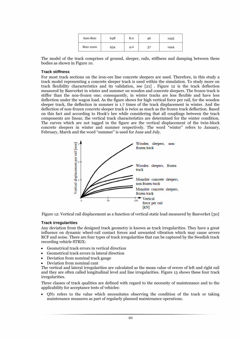
For most track sections on the iron-ore line concrete sleepers are used. Therefore, in this study a track model representing a concrete sleeper track is used within the simulation. To study more on track flexibility characteristics and its validation, see [21] . Figure 12 is the track deflection measured by Banverket in winter and summer on wooden and concrete sleepers. The frozen track is stiffer than the non-frozen one; consequently, in winter tracks are less flexible and have less deflection under the wagon load. As the figure shows for high vertical force per rail, for the wooden sleeper track, the deflection in summer is 1.7 times of the track displacement in winter. And the deflection of non-frozen concrete sleeper track is twice as much as the frozen track deflection. Based on this fact and according to Hook’s law while considering that all couplings between the track components are linear, the vertical track characteristics are determined for the winter condition. The curves which are not tagged in the figure are the vertical displacement of the twin-block concrete sleepers in winter and summer respectively. The word “winter” refers to January, February, March and the word “summer” is used for June and July.

Figure 12: Vertical rail displacement as a function of vertical static load measured by Banverket [30]

Track irregularities

Any deviation from the designed track geometry is known as track irregularities. They have a great influence on dynamic wheel-rail contact forces and unwanted vibration which may cause severe RCF and noise. There are four types of track irregularities that can be captured by the Swedish track recording vehicle STRIX:

Geometrical track errors in vertical direction

Geometrical track errors in lateral direction

Deviation from nominal track gauge

Deviation from nominal cant The vertical and lateral irregularities are calculated as the mean value of errors of left and right rail and they are often called longitudinal level and line irregularities. Figure 13 shows these four track irregularities.

Three classes of track qualities are defined with regard to the necessity of maintenance and to the applicability for acceptance tests of vehicles:

QN1 refers to the value which necessitates observing the condition of the track or taking maintenance measures as part of regularly planned maintenance operations.

11

QN2 refers to the value which requires short term maintenance action.

QN3 refers to the value which, if exceeded, leads to the track section being excluded from the acceptance analysis because the track quality encountered is not representative of usual quality standards.

Figure 13: Four types of track irregularities

Table 4: Permissible standard deviations for different speed intervals in longitudinal and line levels for track classes QN1 and QN2 according to UIC Code 518

Standard deviation for

longitudinal level (mm)

Standard deviation for

line level (mm)

Vehicle speed intervals (km/h) QN1 QN2 QN1 QN2

0 < v ≤ 80 2.3 2.6 1.5 1.8

80 < v ≤ 120 1.8 2.1 1.2 1.5

120 < v ≤ 160 1.4 1.7 1.0 1.3

160 < v ≤ 200 1.2 1.5 0.8 1.1

200 < v ≤ 300 1.0 1.3 0.7 1.0

The details of track irregularity classification as function of vehicle speed are presented in Table 4. The values are calculated for every 100 m of the iron-ore line and the corresponding statistics for track irregularity measured on iron-ore line in 2012 are presented in Table 5.

Table 5: Track quality distribution on iron-ore line according to UIC 518; Maximum speed of 80 km/h assumed

Track quality

classes

Definition of the classes Distribution

of each class

Recommended

by UIC 518

QN ≤QN1 Sections with good track standard 29% Should be > 50%

QN1<QN≤ QN2 Regularly planned maintenance operations

23% Should be < 40%

QN2<QN ≤QN3 Short term maintenance action 43% Should be < 10%

12

QN>QN3 Sections to be excluded from the analysis

5%

Should be = 0%

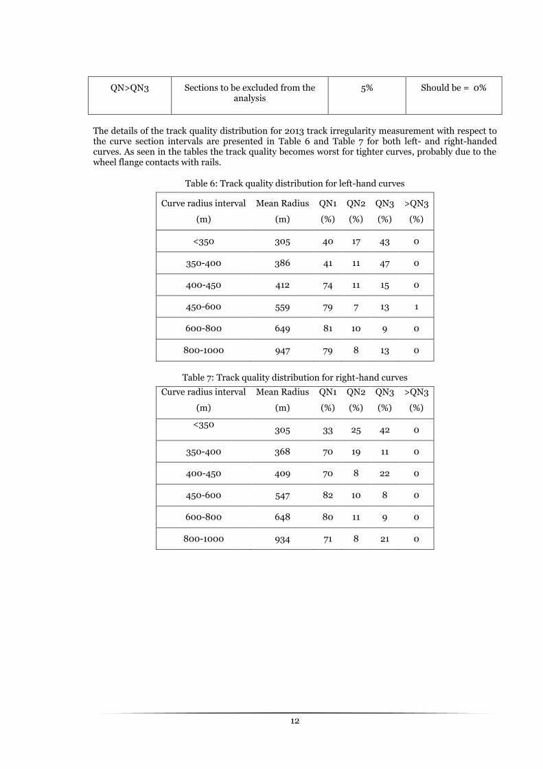
The details of the track quality distribution for 2013 track irregularity measurement with respect to the curve section intervals are presented in Table 6 and Table 7 for both left- and right-handed curves. As seen in the tables the track quality becomes worst for tighter curves, probably due to the wheel flange contacts with rails.

Table 6: Track quality distribution for left-hand curves

Curve radius interval

(m)

Mean Radius

(m)

QN1

(%)

QN2

(%)

QN3

(%)

>QN3

(%)

<350 305 40 17 43 0

350-400 386 41 11 47 0

400-450 412 74 11 15 0

450-600 559 79 7 13 1

600-800 649 81 10 9 0

800-1000 947 79 8 13 0

Table 7: Track quality distribution for right-hand curves

Curve radius interval

(m)

Mean Radius

(m)

QN1

(%)

QN2

(%)

QN3

(%)

>QN3

(%)

<350 305 33 25 42 0

350-400 368 70 19 11 0

400-450 409 70 8 22 0

450-600 547 82 10 8 0

600-800 648 80 11 9 0

800-1000 934 71 8 21 0

13

44 Wheel-rail interaction

The wheel-rail contact problem

Briefly, the contact problem is to find the tangential and the normal pressure distribution and size and shape of the contact area for either known deformations or known loads or a combination of these. There have been a large number of studies in the field of wheel-rail contact mechanics, which are reviewed in [28] . However, in this section the two most common and widely used theories are presented which are also used in GENSYS (Hertzian and Kalker’s simplified theories). Considering the half-space assumption when the bodies of contact deform like infinite half-spaces we demand that:

The size of the contact area is considerably smaller than typical dimensions of the bodies and

The contact should be non-conforming (tread contact).

Boussinesq [23] and Cerruti [24] have presented the relation between the surface tractions and their corresponding displacements in the bodies of contact via the so called influence functions. The derivation of these formulae can be found in Gladwell [25] and Love [26] . Moreover, if the bodies in contact are quasi-identical:

, (3)

where, , and , are the shear modulus and Poisson ratio of the first and second body. It can be shown; that the displacements in the tangential plane are not influenced by the normal traction and the displacement in the normal direction is not influenced by the tangential traction. Thus, in an approach called “the Johnson process” the normal and tangential contact problem is decoupled and the contact problem is formulated as follows:

Determining the normal pressure distribution in absence of the friction and thus the tangential traction considering perfectly smooth surfaces (Normal problem),

Determining the tangential traction distribution when they are bound by the friction coefficient times the normal pressure (Tangential problem).

Using the above assumptions, Hertz presented his method to solve the normal contact problem (today known as Hertzian solution) [27] . He also had to use some other assumptions to simplify his problem such as:

The bodies in contact are homogeneous, isotropic, and linearly elastic. Linear kinematic hardening is also assumed (constant range between yield in tension and compression with equal strain hardening rates).

Displacements and strains are small.

The curvatures of the surfaces in the vicinity of the contact area are constant to be able to calculate the shape and size of the contact area.

Considering quadratic functions for each surface near the contact (constant curvature assumption), elliptic contact area and a semi-ellipsoidal pressure distribution, Hertz calculated the pressure distribution over the contact patch,

, (4)

where and are the semi-axes of the elliptic contact area and is the maximum contact pressure,

. (5)

The semi-axes of the contact ellipse are functions of the geometries of the bodies and the applied force.

To solve the tangential contact problem, Kalker, among other theories, developed his linear theory [29] . In which is assumed that except the trailing edge the entire contact patch is covered by the stick region. This is due to the fact that the creepages are so small that the tractions never violates

14

the traction bound. Then, at the trailing edge the traction suddenly drops to zero. In this theory there is a linear relation between the creepages and creep forces as well as between the spin and the moment as shown in Equations 6, 7 and 8.

, (6)

, (7)

. (8)

where, and are the tangential creep forces, , and are the longitudinal, lateral and spin

creepages respectively, is the shear modulus and are the so-called Kalker coefficients. The

Kalker coefficients are calculated and tabulated in [29] as they are only functions of Poisson’s ratio and the contact ellipse semi-axes ratio . Kalker introduced another theory called the simplified theory. He used the Winkler bed theory to calculate the contact area, where an elastic foundation is introduced as a mattress with vertical springs independent of each other in a way that in compression they will not affect their neighbouring springs, cf. Figure 14.

Figure 14: Winkler elastic foundation approach

Therefore, due to Hooke’s law the displacements are linearly proportional to the traction,

, (9)

where, and are the displacement differences between the bodies in contact in longitudinal and lateral directions, and are tangential tractions and is the flexibility of the Winkler bed

springs.

In steady-state rolling the relative slip velocity in x and y directions, , is calculated by,

. (10)

In the full adhesion condition (the linear theory) no slip will occur,

. (11)

Thus,

, (12)

and likewise,

, (13)

where and are arbitrary functions of y that arise after the integration. In the simplified theory to determine these functions, Kalker has used the fact that at the leading edge the traction starts to build up from zero and grows with constant stress gradient through the contact until it reaches the bound and it stays at the bound level. Thus, the traction is zero only outside the contact area and at the leading edge,

, (14)

where is the semi-axis of the elliptic contact area at leading edge.

Consequently, the forces calculated by simplified Kalker theory will be,

, (15)

15

. (16)

Note that the sign of the creep forces is always opposite to the sign of the corresponding creepages. The flexibility is then calculated by comparing the results of the simplified Kalker Equations (15) and (16) and the linear (Exact) theory calculated by the true theory of elasticity Equations (6) and (7). Note that the effect of spin is considered in the lateral creep force. Moreover, Kalker presented a mathematical algorithm called FASTSIM to solve the tangential problem in the general case where there is no need of pre-calculated tables or neglecting the spin based on the simplified theory which is widely used in vehicle dynamic simulations.

Creepage and spin

As seen in Equations (15) and (16), the spin and creepages have great influence on the contact forces. The contact forces are then affect the contact position on wheel and rail and consequently the size and shape of the contact patch. Here it is useful to briefly mention how these creepages and spin are calculated via the dynamics of a rolling wheelset on a track. Details of how to derive these equations and terms are presented in [30] Chapter 8.

Figure 15: The schematic of a wheelset on rails

If is a small angle between the y-axis and the wheelset, the lateral creepage depends on

Lateral velocity of the centre of the wheelset .

Therefore, the dimensionless lateral creepage would be

, (17)

where, is the rolling velocity

. (18)

is the wheel radius and is the angular velocity of the wheel.

The Longitudinal creepage is determined by

Difference of the rolling radii

Rotation of the wheelset about the z axis

Braking or acceleration

Note that the signs of the longitudinal creepages are different on the left and the right wheels (in absence of braking or acceleration) cf. equations 19 and 20.

, (19)

. (20)

16

Here is half the distance between the contact points on the left and the right wheels.

Finally, the spin is a function of kinematic and geometric spin as shown in Equations (21) and (22).

, (21)

. (22)

Wheel and rail profiles

GENSYS pre-calculates six wheel-rail contact geometry functions: contact position, wheel rolling radius, contact angle, wheel lift, lateral curvature, lateral position of the contact point on wheel and lateral position of the contact point on rail. The program steps from right to left on the wheel profile, and calculates the contact point functions for all relative lateral displacements between wheel and rail. The wheels of the iron-ore wagons have the so-called WP4 profile and the wheels of the locomotives have the so-called WPL9 profile. The rail profile distributions, however, are more complicated. On the Norwegian side of the line for the curve sections with radii below 600 m the higher rail has the MB1 and the lower rail has the MB4 rail profiles. The MB4 rail profile is the standard UIC60 rail with a slight gauge corner relief. This moves the contact point slightly towards the field side and leads to a higher rolling radius difference and better steering performance. A comparison between the implemented rail profiles of the line is shown in Figure 16. The MB1 rail profile is more ground at the gauge corner to avoid any contact and consequently head checking on the corner of the rails. For the track sections having radii above 600 m including the straight track sections, the MB4 rail profile is used for both the high and low rails. On the Swedish side of the line for all curve sections the MB1 and UIC60 rail profiles are used for the high and low rails respectively. On straight lines both rails have either MB4 or UIC60 rail profiles. The distribution of the rail profiles along the entire line is shown in Table 8.

Figure 16: Comparison between the rail profiles (rail inclination: 1/30)

Table 8: The nominal rail profiles along the iron-ore line

Curve radius <600 Curve radius >600 Straight line

High rail Low rail High rail Low rail High rail Low rail

Norway MB1_assymetric MB4 MB4 MB4 MB4 MB4

Sweden MB1 UIC60 MB1 UIC60 MB4,

UIC60

MB4,

UIC60

Any combination of the mentioned wheel profiles (WP4 and WPL9) and each of the mentioned rail profiles produces a unique wheel-rail geometry function. Here we compare the equivalent concities for each combination mentioned in Table 8 for the nominal track gauge (1435 mm), and the average track gauge of the line (1445 mm). As shown in Figure 17, at nominal track gauge the highest equivalent conicity is achieved if both rails have the UIC60 rail profile while at the average track gauge of the line (1445 mm) using MB4 rail profiles for both rails gives the highest equivalent

0 5 10 15 20 25 30

-10

-8

-6

-4

-2

mm

mm

MB1

MB4

UIC60

17

conicity. Generally, higher equivalent conicity leads to a greater rolling radius difference and a better steering performance in curves. A wheel-rail profile combination with low values of equivalent conicity usually helps the stability of the vehicle at higher speeds.

Figure 17: Equivalent conicity of the wheel-rail profile combinations as a function of lateral displacement (mm) of the wheelset

It is also possible to see the contact positions on the wheel and rail depending on the lateral displacement of the wheelset. As it is seen in the figure UIC60 gives the most distributed contact positions on the wheel and rail and the gauge corner relief MB1 rail profile gives the most condensed contact positions. Moreover, both the MB4 and MB1 rail profiles give two-point contacts at the outer wheels in tight curves, since there is no material at the corner of the rails. This, on one hand, will divide the load on two different contact points and avoids the concentrated load on one point leading to safer transferring the load through the fastenings and to the ballast, especially when the fastenings are not strong enough or not positioned correctly. Having two-point contacts on the outer wheel, on the other hand, decreases the steering ability. Since the directions of the longitudinal creep forces would be different on the two contact patches the total resulting steering forces decrease. Consequently, higher attack angles are predicted in these cases.

Wheel-rail friction coefficient

The proportionality factor of the normal load and the resistance force in sliding is called the friction coefficient. The dynamic behaviour of the vehicle, among many other things, strongly depends on the coefficient of friction. On one hand a high friction coefficient is needed for adequate adhesion conditions and better radial steering. On the other hand higher friction leads to larger creep forces and will increase the risk of RCF. The coefficient of friction greatly depends on the weather, rail temperature, passing axle number and tribological surface conditions like roughness, hardness etc. It may vary dramatically during a day from morning to night. In [31] the proportionality of the friction level to the rail temperature (among other parameters like humidity of the weather) is experimentally investigated. Usually from very humid to extremely dry weather, the friction coefficient can vary from 0.2 to 0.75. In cold dry climate conditions, as the water content in air reduces significantly, the wheel-rail friction coefficient increases.

18

55 Validation of the three-piece bogie model

The simulation model against the available measured forces and accelerations is validated. There are two types of measurement data available from the iron-ore line. One is the track-based strain gauge measurement mostly for online monitoring the vehicle performance in order to detect wheel failures. The other one is the measurement via accelerometers attached to the vehicle. The latter type of measurement has been performed by Interfleet Technology during the summer of 2004 and the winter of 2011.

Vehicle-based measurement

Bogojevic [16] , compared the calculated and measured carbody accelerations in vertical and lateral direction for both empty and loaded conditions. Here some more results are presented, cf. Figure 18-21. The friction level is assumed to be 0.4and the vehicle speed is 60 km/h for all calculations. The 2004 measurement data is used. Both the measured and calculated results are filtered with cut-off frequency of 20 Hz.

Figure 18: Measured (top) and simulated (bottom) lateral acceleration of empty wagon above leading bogie on tangent track

19

Figure 19: Measured (top) and simulated (bottom) vertical acceleration of empty wagon above leading bogie on tangent track

Figure 20: Measured (top) and simulated (bottom) lateral acceleration of loaded wagon above leading bogie on tangent track

20

Figure 21: Measured (top) and simulated (bottom) vertical acceleration of loaded wagon above

leading bogie on tangent track

Track-based measurement

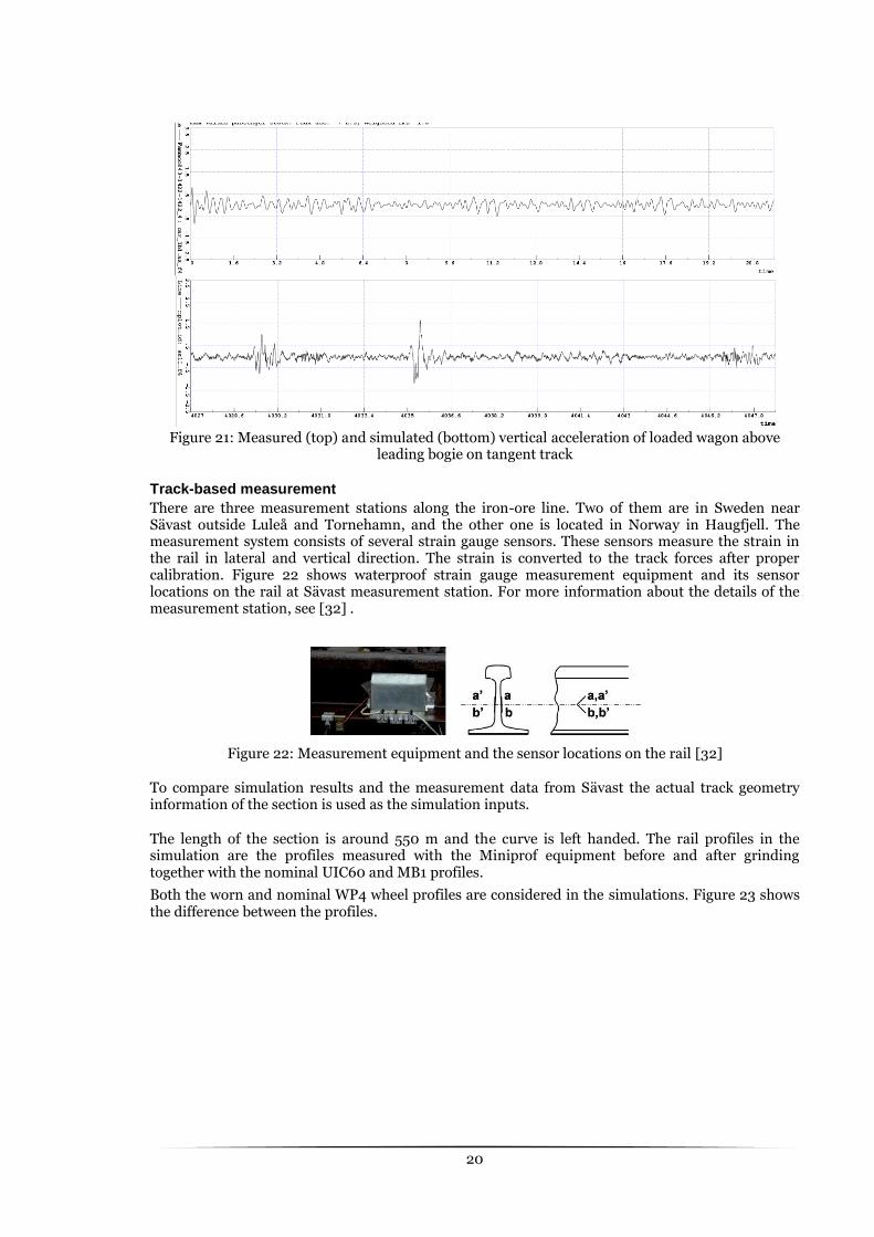
There are three measurement stations along the iron-ore line. Two of them are in Sweden near Sävast outside Luleå and Tornehamn, and the other one is located in Norway in Haugfjell. The measurement system consists of several strain gauge sensors. These sensors measure the strain in the rail in lateral and vertical direction. The strain is converted to the track forces after proper calibration. Figure 22 shows waterproof strain gauge measurement equipment and its sensor locations on the rail at Sävast measurement station. For more information about the details of the measurement station, see [32] .

Figure 22: Measurement equipment and the sensor locations on the rail [32]

To compare simulation results and the measurement data from Sävast the actual track geometry information of the section is used as the simulation inputs.

The length of the section is around 550 m and the curve is left handed. The rail profiles in the simulation are the profiles measured with the Miniprof equipment before and after grinding together with the nominal UIC60 and MB1 profiles.

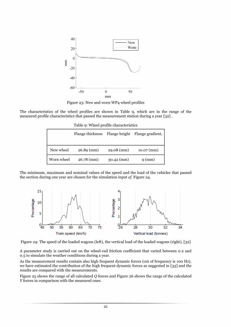
Both the worn and nominal WP4 wheel profiles are considered in the simulations. Figure 23 shows the difference between the profiles.

21

Figure 23: New and worn WP4 wheel profiles

The characteristics of the wheel profiles are shown in Table 9, which are in the range of the measured profile characteristics that passed the measurement station during a year [32] .

Table 9: Wheel profile characteristics

Flange thickness Flange height

Flange gradient,

New wheel 26.89 (mm) 29.08 (mm) 10.07 (mm)

Worn wheel 26.78 (mm) 30.42 (mm) 9 (mm)

The minimum, maximum and nominal values of the speed and the load of the vehicles that passed the section during one year are chosen for the simulation input cf. Figure 24.

Figure 24: The speed of the loaded wagons (left), the vertical load of the loaded wagons (right), [32]

A parameter study is carried out on the wheel-rail friction coefficient that varied between 0.2 and 0.5 to simulate the weather conditions during a year.

As the measurement results contain also high frequent dynamic forces (cut of frequency is 100 Hz), we have estimated the contribution of the high frequent dynamic forces as suggested in [33] and the results are compared with the measurements.

Figure 25 shows the range of all calculated Q forces and Figure 26 shows the range of the calculated Y forces in comparison with the measured ones.

22

Figure 25: Comparison between measured and calculated vertical forces. a) left wheel, b) right wheel. The blue and red lines show the maximum and minimum of the calculated forces while the background grey diagrams show the distribution of the measured forces in a year.

Figure 26: Comparison between the measured and calculated lateral forces. a) left wheel, b) right wheel, the blue and red lines show the maximum and minimum of the range of the calculated forces while the background diagrams show the distribution of the measured forces in a year.

As can be seen in the figures there is a fairly good agreement between the simulation results and the measurements. The highest deviation occurred at the outer wheel of the leading bogie. The vehicle usually runs with flange contact at these conditions. Usually the flange contact (especially for worn wheels and rails with more conforming contact) violates the half-space assumption in the Hertzian theory which may lead to non-realistic results.

23

66 Wheel damage mechanisms

From the tribologic point of view, damage to a solid surface involving progressive loss of material and relocation of material when two surfaces are interacting via a relative motion, is called wear. How a material wears not only on the nature of the material but also depends on other elements of the tribo-system such as geometry of contacting pairs, surface topography, loading, lubrication and environment. The mechanisms causing such damage usually are complicated and most of the time it is not possible to distinguish one from another. In [34] , approximately, 60 terms describing wear behaviour and mechanisms are listed. Some of the most important wheel-rail related mechanisms are listed below.

Abrasive wear: wear caused by rough and hard surfaces sliding on each other or wear caused by hard particles trapped between two surfaces like hard oxide debris.

Adhesive wear: wear caused by shearing of junctions formed between two contacting surfaces, sometimes used as a synonym for dry sliding wear.

Chemical wear (Corrosive wear): wear caused by formation of any oxide or other components on surfaces due to chemical reaction of the surfaces with the environment.

Erosive wear: Wear due to relative motion of contact surfaces while a fluid containing solid particles is between the surfaces.

Rolling contact fatigue (RCF): caused by cyclic stress variations leading to fatigue of the materials. Generally resulting in the formation of sub-surface and deep-surface cracks, material pitting and spalling.

Kimura [35] studies adhesive wear and RCF and concludes that both phenomena have elemental processes in common. In this study the term “wear” is used for adhesive wear otherwise the complete term of the mechanism is mentioned. Note that the term “mechanical wear” is also used for abrasion, erosion and adhesion.

Wear modelling

Published research and studies in wear modelling usually have three approaches:

field measurements,

laboratory tests and

theoretical prediction models.

Most of the field measurements have addressed the effect of lubrication on wear such as [36] and [37] .

Archard [38] took the idea of the adhesive wear definition and found that the volume of material removed by wear per sliding distance (W) is proportional to the quotient of the pressure (p) and the hardness (H) of the softer material. The proportionality factor is called the wear coefficient (k)

. (23)

The wear coefficient depends on the governing wear mechanisms. Archard validated his model by determining the wear rates for different material pairs by pin-on-disk tests.

Lim and Ashby [39] have performed large amounts of laboratory tests and introduced wear maps where the wear coefficient is plotted as a function of sliding velocity and the nominal pressure (normal load divided by the nominal contact area). The wear map corresponding to medium carbon steel, based largely on pin-on-disc data, is generally divided into two main regions of mechanical and chemical wear, cf. Figure 27. The mechanical wear occurs at low sliding velocities where the wear coefficient is more a function of nominal pressure than the velocity. The chemical mechanism occurs at higher sliding velocities (above 1 m/s). The mechanical part contains three regions of mild and severe wear together with a transition area in between. Childs [40] has suggested a wear map for the mechanical wear mechanism where the wear coefficient is a function of the asperities attack angle and the relative strength of the interfaces. The chemical part of the map, however, contains of two regions: mild and severe oxidational wear. As seen in the figure mild oxidation could even be

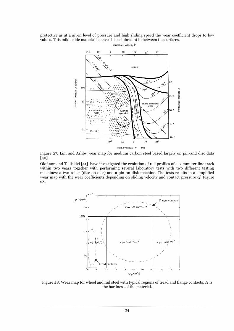
24

protective as at a given level of pressure and high sliding speed the wear coefficient drops to low values. This mild oxide material behaves like a lubricant in between the surfaces.

Figure 27: Lim and Ashby wear map for medium carbon steel based largely on pin-and disc data [40] .

Olofsson and Telliskivi [41] have investigated the evolution of rail profiles of a commuter line track within two years together with performing several laboratory tests with two different testing machines: a two-roller (disc on disc) and a pin-on-disk machine. The tests results in a simplified wear map with the wear coefficients depending on sliding velocity and contact pressure cf. Figure 28.

Figure 28: Wear map for wheel and rail steel with typical regions of tread and flange contacts; H is the hardness of the material.

25

In a different approach McEven and Harvey [42] using a full-scale wheel-on-rail-wear rig, proposed a linear relation between the wear rate and the dissipated energy per unit distance rolled per unit area adjusted with a constant off-set term, . The energy dissipation per unit distance area is the creep forces times the creepages added to the moment times the spin in the contact patch. The proportionality factor is expected to be function of wheel and rail material .They also predicted two wear regimes, i.e. mild (tread contact) and severe (flange contact) wear.

, (24)

. (25)

sometimes is called the wear number. In another study [43] the authors suggested a simple

relationship between the material loss and the energy dissipation:

(26)

(27)

(28)

where, D is diameter of the wheel in millimetres.

Krause and Poll [44] reviewed several other test results and investigations regarding the proportionality of the wear rate to the longitudinal creepage, normal force and sliding distance. They concluded that the volume of material loss ( ) is proportional to the friction work

, (29)

, (30)

where is the sliding distance. The proportionality factor is and it depends on the environmental conditions such as the humidity, the material of contacting surfaces and the temperature of the contact patch. The temperature itself is proportional to the frictional power

, (31)

where is the speed. Krause and Poll also concluded that it is difficult to derive a simple mathematical wear law because:

different parameters are affecting each other. For example the frictional work affects the

surface temperature which changes the tribology of the surfaces and material behaviour.

different mechanisms are involved in a wear process.

Prediction of profile evolution

Several authors have investigated and developed wheel wear prediction tools. Some of them are reviewed in this section. Note that the studies which are mentioned here have neglected the plastic deformation of the material and focused on the uniform wear.

Kalker [45] has developed a method to predict the wheel profile evolution considering that the material loss is proportional to the frictional work. Proportionality factors were gained from field studies. His method was only applied on the tread contact and no flange wear is reported. As he has used Hertzian contact and the simplified theory for his calculations it was not possible to predict severe wear on the wheel profile as the wheel gets a hollow shape and the contact becomes more conforming. No comparison between measurements and calculations are mentioned.

Pearce and Sherratt [46] developed their prediction method using the energy approach where the amount of material loss is proportional to the energy dissipation. The values of the wear coefficients are taken from [43] . In order to validate the model they compared the development of the

26

equivalent conicity over the running distance from both simulation and measurement; the conclusion was that only a qualitive judgment is possible.

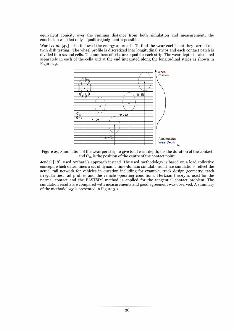
Ward et al. [47] also followed the energy approach. To find the wear coefficient they carried out twin disk testing. The wheel profile is discretized into longitudinal strips and each contact patch is divided into several cells. The numbers of cells are equal for each strip. The wear depth is calculated separately in each of the cells and at the end integrated along the longitudinal strips as shown in Figure 29.

Figure 29, Summation of the wear per strip to give total wear depth; t is the duration of the contact and Cpw is the position of the centre of the contact point.

Jendel [48] used Archard’s approach instead. The used methodology is based on a load collective concept, which determines a set of dynamic time-domain simulations. These simulations reflect the actual rail network for vehicles in question including for example, track design geometry, track irregularities, rail profiles and the vehicle operating conditions. Hertzian theory is used for the normal contact and the FASTSIM method is applied for the tangential contact problem. The simulation results are compared with measurements and good agreement was observed. A summary of the methodology is presented in Figure 30.

27

Figure 30: Methodology of the wheel wear prediction tool developed by Jendel [48]

Enblom [49] has used the same methodology as Jendel. However, he also included the elastic strain in the sliding velocity assessment, cf. Equation (10). He also extended the simulation set with simulation of braking.

Rolling contact fatigue

The current wear models do not include the role of RCF. However, the trade of between wear and RCF is of great interest. In [50] , the implementation of emerging technologies for the prediction of wheel surface deterioration in an engineering environment is summarized. In this section it is tried to touch the concept and theories of RCF.

Every material subjected to repeated rolling contact loads response in one of the following four ways as shown in Figure 31:

a. Perfectly elastic. If the load is sufficiently small so that no part of the material can reach the elastic limit, the response will be perfectly elastic.

b. Elastic shakedown. If the load exceeds the elastic limit in the first few cycles there will be a small plastic deformation. However, due to the changes caused by the plastic flow (residual stresses, strain hardening and more conforming contact) the steady state remains elastic. The maximum load which allows the material to be in this regime is called shakedown limit. Note that the material is subjected to high-cycle fatigue (HCF) and it is expected to have cracks in the long term.

c. Plastic shakedown. The steady state consists of a closed plastic stress-strain loop. In this regime the material is subjected to so-called low cycle fatigue (LCF).

d. Ratchetting. The plastic deformation will remain unstable and there will be an incremental strain growth at each load cycle. Here, the surface of the material soon will be subjected to cracks.

28

Figure 31: Material response to cyclic loading [50]

Johnson [50] used the Von Mises yield criterion and developed a shakedown map in line contact for a perfectly plastic and kinematically hardening material which is widely used in detecting RCF probabilities in railway wheels and rails. The shakedown map is presented in Figure 32.

Figure 32: Shakedown map

As can be seen in Figure 32, for friction levels approximately above 0.3 of high levels of load surface initiated fatigue will be developed. Below this level subsurface flow will occur. An engineering model for RCF risk assessment is developed by Ekberg in [52] based on the shakedown theory cf. Figure 33 (left). Surface initiated fatigue is often characterized as low cycle fatigue and it usually happens when the plastic deformation remains unstable and the strain accumulates until the ductility of the material is exhausted (ratchetting). The location of the points in the shakedown diagram is a function of, firstly, the traction coefficient ( )

, (32)

29

where is the normal contact force, and are longitudinal and lateral creep forces respectively.

Secondly, it depends on the normalized vertical load ( ) which is the maximum contact pressure ( ) divided by the material yield stress in shear ( )

. (33)

The boundary curve for surface plasticity is denoted by BC and calculated as

. (34)

The horizontal distance between the working points and the BC line yields

. (35)

Positive values of represent the ratchetting part of the shakedown diagram resulting in

surface initiated fatigue. The area below the curve in Figure 33 (right) represents the depth of

the ratcheted working points and is particularly used as an index of RCF severity in this study of the influence of the wheel-rail friction coefficient. Here the number of the ratchetted points over the whole number of working points is called RCF probability. Figure 33 (right) shows the typical values of as a function of time where the vehicle is negotiating a curve. In the figure the positive

values are indicated as “Area with risk of RCF”. The negative values are valid for straight track, while the positive values occur when the vehicle is running in the curve.

The longitudinal and lateral traction coefficients are presented in the following form in this study:

, (36)

. (37)

Figure 33: a simpler Shakedown diagram (left) and FIsurf curve (right).

30

77 Summary of the papers

Paper A Wheel damage on the Swedish iron-ore line investigated via multibody simulation

The paper presents some details and a general summary of the three-piece bogies simulation model. The track geometries and irregularities are discussed and some statistics from the iron-ore line are presented. Moreover, after discussing the rail profiles and wheel-rail friction variations, the theory behind the surface initiated RCF is described via the concept of shakedown diagram. During a series of parameter studies it is concluded that RCF mostly occurs in curve sections with radii below 450 m. Improvement of the lubrication policies is suggested especially on the Norway part of the line. Moreover, it is shown that track degradation plays an important role in initiating the cracks. Simulation results show that the track stiffness is not the main concern in case of RCF cracks. However, the study also confirms the significant impact of the wheel-rail friction coefficient on RCF. Good agreement between the predicted location of cracks and the observed ones in field is achieved.

Paper B Prediction of RCF and Wear Evolution of Iron-Ore Locomotive Wheels

The summary of the project background is discussed in the introduction of the paper. Then, a literature review of previous works on wear and RCF is presented. Moreover, the employed wear and RCF calculation methodologies are described. As locomotives are equipped with a flange lubrication system, both lubricated and non-lubricated conditions are considered in the simulations. To include the traction effects on the wheel damages, total resistance forces for each of the simulation cases are calculated. Both the impacts of lubrication and tractive forces on RCF and wear are described via examples. To consider the effect of wear on RCF, a method presented. This method is based on the previous works on modifying the calculated RCF index by the corresponding wear number. Good agreement is achieved when comparing the simulated and measured worn profiles. Moreover, comparing the calculated and observed RCF locations, it is concluded that in reality the vehicle lubrication system is, at least partly not performing as it is expected. The procedure is repeated for two new proposed wheel profiles to choose one for the field tests. These wheel profiles are designed in order to reduce the number of wheel damages. Finally, one of the profiles is suggested to be better than the other one because of producing milder wear and RCF in long term.

31

88 Future work

As continuation of the current study on wear and RCF prediction it is desirable to repeat the calculation for the iron-ore wagon wheels. This includes an analysis of when, during the wheel life, the highest RCF probability occurs. For the wagon model no traction forces will be included. However, as the wagons are equipped with pneumatically actuated tread brakes the influence of braking on material removal needs to be estimated via calculating the braking force for each simulation case considering the topography of the line, the amount of braking by the locomotives and the running resistance from curving, aerodynamics and mechanical resistance.

Moreover, in order to improve the current wheel profile optimisation methods, it will be tried to include wear prediction into an optimisation process. However, this is a challenging issue. The average calculation time for simulating wear on the wheels for c.a. 300 km is more than one hour even on powerful computers with the ability of handling parallel simulations. Thus, it is very challenging to use this technique in a wheel profile optimization process where the long term stability of the profile is one of the goal functions. Therefore, there is a need to find a reliable and fast method that can replace the current wear calculation method.

32

99 References

[1] V. Terrey Hawthorne, P. E., Ceng, Recent improvements to three-piece trucks, Proc. of Railroad Conference. (1996)

[2] P. A. Jönsson, Freight wagon running gear-a review. TRITA-FKT Report 2002:35. KTH Royal Institute of Technology, Stockholm, (2002).

[3] H. Scheffel, Unconventional bogie designs – their practical basis and historical background, Vehicle System Dynamics, 24, pp. 497-524 (1995).

[4] A Orlova, Y. Romen, Refining the wedge friction damper of three-piece freight bogies, Vehicle System Dynamics, 46, pp. 445-455 (2009).

[5] A Orlova, E. Rudakova, Comparison of different types of friction wedge suspensions in freight wagons. Proc. Of 8th International Conference on Railway Bogies and Running Gears, Budapest (2010).

[6] L. H. Ren, G. Shen, Y. S. Hu, A test-rig for measuring three-piece bogie dynamic parameters applied to a freight car application, Vehicle System Dynamics, 44, pp. 853-861 (2006).

[7] Yu. Boronenko, A. Orlova and E. Rudakova, Influence of construction schemes and parameters, Vehicle System Dynamics, 44(1), 2006, pp. 402-414.

[8] N. Wilson, H. Wu, H. Tournay, C. Urban, Effects of wheel/rail contact patterns and vehicle parameters on lateral stability, Vehicle System Dynamics, 48, , pp. 487-503 (2010).

[9] S. A. Schwam, Truck hunting in the three-piece freight car truck, Proc. the Economics and Performance of Freight Car Trucks Conference, pp. 77-91 (1983).

[10] A. Orlova, Identification of parameters for spatial wedge system implemented in freight bogie design, Abstracts of 10th Mini Conference on Vehicle System Dynamics, Identification and Anomalies, pp. 30-31 (2006).

[11] K. Round, C. Pasta, Warp characteristics of bulk commodity suspensions American steel foundries SSRM truck, Technology Digest Timely Technology Transfer (2003).

[12] J. Tunna, G. F. M. Dos Santos, E. J. Kina, Theoretical and service evaluation of wheel performance on frame brace trucks, Proc. 9th IHHA Conference, pp. 409-415, (2009).

[13] H. Scheffel, H. Kovtun, O. Markova, W. Kik, Radial arm: A Retrofit kit to improve the dynamics of freight car bogies, Rail vehicle dynamics and associated problems, pp. 123-134, (2005).

[14] A. Berghuvud, A. Stensson, Dynamic behaviour of ore wagons in curves at Malmbanan. Vehicle System Dynamics. Special Issue: Computer Simulation of Rail Vehicle Dynamics, Vol. 30, pp. 271-284, (1998).

[15] A Berghuvud, A. Stensson, Prediction of lateral wheel-rail contact forces for ore wagons with three-piece bogies. Proc. Of VSDIA,6th Mini Conference on Vehicle System Dynamics, Identification and Anomalies, Budapest, pp 161-170 (1998).

[16] N. Bogojevic, P. Jönsson, S. Stichel. Iron ore transportation Wagon with three-piece bogies simulation model and validation, Proceeding of International Conference on Heavy Machinery 7 (1), pp 39-44 (2011).

[17] A. Orlova, Y. Boronenko, The influence of the condition of three-piece freight bogies on wheel flange wear: simulation and operation monitoring, Vehicle System Dynamics, Vol. 48, pp 37-53 (2010).

[18] M.A Howard, R.D. Fröhling, C.R. Kayser, Validation simplification and application of a computer model of load sensitive damping in three-piece bogies, Proc. IHHA 2, pp. 699-713 (1997).

[19] J. Gardner, J Cusumano, Dynamic model of friction wedge dampers, Proc. IEEE/ASME Joint, pp. 65-69 (1997).

[20] Y. Q. Sun, C. Cole, Vertical dynamic behaviour of three-piece bogie suspensions with two types of friction wedge, Multibody Syst. Dyn. 19, pp. 365-382 (2008).

[21] N. Chaar, M. Berg, Simulation of vehicle-track interaction with flexible wheelsets, moving track models and field tests. Vehicle System Dynamics, Vol. 44 (1), pp 921-931. (2006).

[22] UIC: Testing and approval of railway vehicles from the point of view of their dynamic behavior –safety –Track fatigue – Ride quality, Code 518 OR, 2nd edition, April (2003).

33

[23] J. Boussinesq, Application des potentiels a l’equilibre et du mouvement des solides elastiques, Paris, Gauthier-Villars (1885).

[24] V. Cerruti, Accademia dei Lincei, Roma. Mem. fs. Mat, (1882). [25] G.M.L. Gladwell, Contact problem in the classical theory of elasticity. Sijethoff and

Noordhoff, Alphen a/d Rijn, the Netherlands, (1980). [26] E. H. Love, A treatise on theory of elasticity. 4th Ed. Cambridge UP, (1926). [27] H. Hertz, Uber die Beruhrung zweier fester, elastischer Körper. Jurnal fur die reine und

angewandte Mathematik, Vol. 92, (1882). [28] M. S. Sichani, Wheel-rail contact modelling in vehicle dynamics simulation, Licentiate thesis

in Vehicle Maritime Engineering, KTH Royal Institute of Technology Stockholm, Sweden 2013

[29] J. Kalker, Rolling contact phenomena- Linear elasticity, CISM Courses and Lectures, Wien, New York: Springer, (2001), pp 1-184.

[30] E. Andersson, M. Berg, S. Stichel, Rail Vehicle Dynamics, KTH Royal Institute of Technology Stockholm.

[31] M. Ishida, T. Ban, M. Takikawa, F. Aoki. Influential factors on rail/wheel friction coefficient. Proceedings of the 6th International Conference on Contact Mechanics and Wear of Rail/Wheel Systems. pp 23-27 (2003).

[32] M. Palo, H. Schunnesson, U. Kumar, Condition monitoring of rolling stock using wheel/rail forces. Insight (Northampton), Vol 54, pp 451-455 (2012),.

[33] P-E Westin, Banavgifter för kund- och samhällsnytta, Report, Trafikverket (The Swedish Transport Authority), (2012)

[34] Ed. P.J. Blau, Glossary of terms, Friction, Lubrication, and Wear Technology Metals Handbook, ASME International, Metals Park, OH: Vol. 18, (1992).

[35] Y. Kimura et al, Wear and fatigue in rolling contact, Wear, Vol. 252, pp 9-16(2002). [36] R. K. Steele, Rail Lubrication: The relation of wear and fatigue, Transportation research

record 1042, pp 24-32, (1985). [37] R. Nilsson, On wear in rolling sliding contacts. TRITA-MMK 2005_ 03, Doctoral Thesis,

Department of Mechanical Design, Royal Institute of Technology (KTH) Stockholm, (2005). [38] J. F. Archard, Contact and rubbing of flat surface, J. Appl. Phys. Vol. 24, 981 (1953) [39] S. C. Lim, M. F. Ashby, Wear mechanisms maps, Acta Metallorgica 35, pp 1-24 (1987). [40] T. H. C. Childs, The mapping of metallic sliding wear, Proc. Instn. Mech. Engrs. C 202, pp

379-395 (1988). [41] U. Olofsson, T. Telliskivi, Wear plastic deformation and friction of two rail steels-a full-scale

test and a laboratory study, Wear: Vol. 254, pp 80-93 (2003). [42] I. J. McEven, R. F. Harvey, Full-scale wheel-on-rail wear testing: comparisons with service

wear and a developing theoretical predictive method. Lubrication Engineering, Journal of the American Society of Lubrication Engineers, Vol. 41, pp 80-88, (1985).

[43] I. J. McEven, R. F. Harvey, Interpretation of wheel/rail wear numbers, British Rail Research report TM VDY 4, (1981).

[44] H. Krause, G. Poll, Wear of wheel-rail surfaces. Wear, Vol. 113, (1986), pp 103-122O [45] Kalker. J. J, Simulation of the development of a railway wheel profile through wear, Wear:

Vol, 150, (1991), pp 355-365 [46] T. G. Pearce, N. D. Sherratt, Prediction of wheel profile wear, Wear: Vol 144 (1991), pp 343-

351 [47] A. Ward, R. Lewis, R.S. Dwyer-Joyce, Incorporating a railway wheel/rail model into multi-

body simulations of wheelset dynamics. Proceeding of the 29th Leeds-Lyon Symposium on Tribology, (2003)

[48] T. Jendel, Prediction of wheel profile wear-comparisons with field measurements, Wear: Vol. 253, pp 89-99,(2002).

[49] R. Enblom, Simulation of wheel and rail profile evolution-wear modelling and validation. TRITA AVE 2004:19, Licentiate Thesis, Department of Aeronautical and Vehicle Engineering, KTH Royal Institute of Technology Stockholm, (2004).

[50] K. L. Johnson, The strength of surfaces in rolling contact, Proc Instn Mech Engrs, Vol. 203 , pp 151-163 (1989).

[51] R. Enblom, S. Stichel. Industrial implementation of novel procedures for the prediction of railway wheel surface deterioration. Wear; 271 (1-2): pp 203-209 (2010).

34

[52] A. Ekberg, E. Kabo, H. Andersson. An engineering model for prediction of rolling contact fatigue of railway wheels. Fatigue and Fracture of Engineering Materials and Structures; Vol. 25, pp 899–909 (2002).

[53] K. Karttunen, E. Kabo, A. Ekberg. A numerical study of the influence of lateral geometry irregularities on mechanical deterioration of freight tracks. Journal of Rail and Rapid Transit; 226 Issue 6: pp 575-586 (2012).

[54] N. Chaar, M. Berg. Vehicle-track dynamic simulation of a locomotive considering wheelset structural flexibility and comparison with measurements. Journal of Rail and Transit; 219: pp 225-238, (2005).

[55] M. C. Burstow. Whole life rail model application and development for RSSB –Continued development of an RCF damage parameter. Rail safety and standards board; Issue 2 Report EATR-S-2004-880 (2004).

[56] A. Ekberg, E. Kabo, K. Karttunen, B. Lindqvist, R. Lundén, T. Nordmark, J. Olovsson, O. Salomonsson, T. Vernersson. Identifying the root causes of damage of the wheels of heavy haul locomotives and its mitigation. Journal of Rail and Rapid Transit, Vol. 228 pp 663-672, (2014).

35

PART II

APPENDED PAPERS A-B