UC RiversideUC Riverside Electronic Theses and Dissertations

TitlePolices for Controlling Groundwater Pollution from Concentrated Animal Feeding Operations

Permalinkhttps://escholarship.org/uc/item/3s10n57k

AuthorWang, Jingjing

Publication Date2012-01-01 Peer reviewed|Thesis/dissertation

eScholarship.org Powered by the California Digital LibraryUniversity of California

UNIVERSITY OF CALIFORNIARIVERSIDE

Polices for Controlling Groundwater Pollution from Concentrated AnimalFeeding Operations

A Dissertation submitted in partial satisfactionof the requirements for the degree of

Doctor of Philosophy

in

Environmental Sciences

by

Jingjing Wang

June 2012

Dissertation Committee:

Professor Kenneth Baerenklau, ChairpersonProfessor Kurt SchwabeProfessor Keith Knapp

Copyright byJingjing Wang

2012

The Dissertation of Jingjing Wang is approved:

Committee Chairperson

University of California, Riverside

Acknowledgments

I would like to express my deepest gratitude to my adviser, Professor Kenneth

Baerenklau, for his outstanding guidance, caring and support throughout my graduate

education at University of California-Riverside. Both of us have an environmental engi-

neering background and thus he has been able to provide me plentiful wonderful help as I

transition to the field of economics. I am honored and fortunate to have him as my adviser.

I am indebted to my committee members, Professors Kenneth Baerenklau, Kurt

Schwabe and Keith Knapp, whose passion for environmental and agricultural economics

has inspired me to take my own passions seriously. This dissertation would not have been

possible without their guidance and encouragement.

I am deeply grateful to Dr. Jirka Šimunek, Dr. John Letey, and Dr. Ariel Dinar

in my department. They took their precious time to contribute many helpful ideas and to

provide much needed expertise, from which this thesis has benefited greatly. I would like

to thank Sunny Sohrabian, an undergraduate intern who helped with data generation.

I would like to acknowledge Dr. Thomas Harter at University of California-Davis,

Dr. Brad Esser, Dr. Michael Singleton and Dr. Steve Carle at Lawrence Livermore National

Laboratory, and Ms. Carol Frate at University of California Cooperative Extension for their

help.

Finally, I would like to thank my family for their love and endless support. I

would also like to thank my friends scattered around the world, especially those who are

pursuing or finishing up their doctorates. It would have been a lonely research world

without their phone calls, emails, and texts from China, Japan, and Europe.

iv

To my parents.

v

ABSTRACT OF THE DISSERTATION

Polices for Controlling Groundwater Pollution from Concentrated AnimalFeeding Operations

by

Jingjing Wang

Doctor of Philosophy, Graduate Program in Environmental SciencesUniversity of California, Riverside, June 2012Professor Kenneth Baerenklau, Chairperson

Animal waste from animal feeding operations (AFOs) is a significant contributor to ni-

trate contamination of groundwater. Some animal waste also contains heavy metals and

salts that may build up in cropland and underlying aquifers. This thesis focuses on pollu-

tion reduction from the largest AFOs, in particular, Concentrated Animal Feeding Opera-

tions (CAFOs), which present the greatest potential risk among all AFOs to environmental

quality and public health. To find cost-effective policies for controlling pollution at the

field level and at the farm level, a dynamic environmental-economic modeling framework

for representative CAFOs is developed. The framework incorporates four models (i.e.,

animal model, crop model, hydrologic model, and economic model) that includes vari-

ous components such as herd management, manure handling system, crop rotation, water

sources, irrigation system, waste disposal options, and pollutant emissions. The opera-

tor maximizes discounted total farm profit over multiple periods subject to environmen-

tal regulations. Decision rules from the dynamic optimization problem demonstrate best

management practices for CAFOs to improve their economic and environmental perfor-

vi

mance. Results from policy simulations suggest that direct quantity restrictions of emis-

sion or incentive-based emission policies are much more cost-effective than the standard

approach of limiting the amount of animal waste that may be applied to fields; reason be-

ing, policies targeting intermediate pollution and final pollution create incentives for the

operator to examine the effects of other management practices to reduce pollution in ad-

dition to controlling the polluting inputs. Incentive-based emission policies are shown to

have advantages over quantity restrictions over multiple years when seasonal or annual

emissions fluctuate either due to inherent operation practices or the accumulation of pre-

cursors to the pollution. My approach demonstrates the importance of taking into account

the integrated effects of water, nitrogen, and salinity on crop yield and nitrate leaching

as well as the spatial heterogeneity of nitrogen/water application. It also suggests that

ecosystem services can play an important role in pollution control and thus deserve more

attention when designing policies.

vii

Contents

Contents viii

List of Figures xi

List of Tables xiii

I Introduction 1

1 Background 21.1 Animal Feeding Operations . . . . . . . . . . . . . . . . . . . . . . . . . . . . 2

1.1.1 AFOs and CAFOs . . . . . . . . . . . . . . . . . . . . . . . . . . . . . . 21.1.2 Environmental and Public Health Impacts . . . . . . . . . . . . . . . 4

1.1.2.1 Water Pollution . . . . . . . . . . . . . . . . . . . . . . . . . 51.1.2.2 Air Pollution and Greenhouse Gases Emissions . . . . . . . 8

1.1.3 California Dairies . . . . . . . . . . . . . . . . . . . . . . . . . . . . . . 81.1.4 California Groundwater Contamination . . . . . . . . . . . . . . . . . 9

1.2 Existing Policy Regime . . . . . . . . . . . . . . . . . . . . . . . . . . . . . . . 111.3 Animal Waste Management . . . . . . . . . . . . . . . . . . . . . . . . . . . . 14

1.3.1 Animal Waste Management Strategies . . . . . . . . . . . . . . . . . . 141.3.1.1 Land Disposal . . . . . . . . . . . . . . . . . . . . . . . . . . 141.3.1.2 Wetland Treatment . . . . . . . . . . . . . . . . . . . . . . . 151.3.1.3 Anaerobic Digester System . . . . . . . . . . . . . . . . . . . 16

1.3.2 Dairy Manure Management in California . . . . . . . . . . . . . . . . 17

2 Literature Review 192.1 Environmental-Economic Analysis for CAFOs . . . . . . . . . . . . . . . . . 192.2 Policy Instruments for Groundwater Protection . . . . . . . . . . . . . . . . . 21

2.2.1 Nitrates in Groundwater . . . . . . . . . . . . . . . . . . . . . . . . . . 212.2.2 Salts in Groundwater . . . . . . . . . . . . . . . . . . . . . . . . . . . . 24

2.3 Summary . . . . . . . . . . . . . . . . . . . . . . . . . . . . . . . . . . . . . . . 25

viii

II Integrated Farm Level Model 26

3 Animal Model 293.1 Herd Growth and Production . . . . . . . . . . . . . . . . . . . . . . . . . . . 29

3.1.1 Herd Dynamics . . . . . . . . . . . . . . . . . . . . . . . . . . . . . . . 293.1.2 Herd Production . . . . . . . . . . . . . . . . . . . . . . . . . . . . . . 313.1.3 Economic Submodel for Herd Production . . . . . . . . . . . . . . . . 31

3.2 Animal Waste . . . . . . . . . . . . . . . . . . . . . . . . . . . . . . . . . . . . 323.2.1 Waste Generation and Management . . . . . . . . . . . . . . . . . . . 323.2.2 Economic Submodel for Waste Management . . . . . . . . . . . . . . 34

4 Crop Model 364.1 Economic Submodel for Crop Production . . . . . . . . . . . . . . . . . . . . 364.2 Irrigation . . . . . . . . . . . . . . . . . . . . . . . . . . . . . . . . . . . . . . . 374.3 Crop Choice . . . . . . . . . . . . . . . . . . . . . . . . . . . . . . . . . . . . . 384.4 Crop Dataset Generation . . . . . . . . . . . . . . . . . . . . . . . . . . . . . . 41

4.4.1 Model selection: HYDRUS-1D . . . . . . . . . . . . . . . . . . . . . . 414.4.2 Model Validation . . . . . . . . . . . . . . . . . . . . . . . . . . . . . . 434.4.3 Model Input . . . . . . . . . . . . . . . . . . . . . . . . . . . . . . . . . 454.4.4 Dataset Generation . . . . . . . . . . . . . . . . . . . . . . . . . . . . . 49

4.5 Crop Response Function Estimation . . . . . . . . . . . . . . . . . . . . . . . 504.5.1 Relative Yield Function . . . . . . . . . . . . . . . . . . . . . . . . . . 514.5.2 Field Emission Function . . . . . . . . . . . . . . . . . . . . . . . . . . 564.5.3 Alternative Function Specification . . . . . . . . . . . . . . . . . . . . 60

5 Hydrologic Model 615.1 Unsaturated Zone . . . . . . . . . . . . . . . . . . . . . . . . . . . . . . . . . 62

5.1.1 Soil Dynamics and Root Zone Supply . . . . . . . . . . . . . . . . . . 625.1.2 Drainage . . . . . . . . . . . . . . . . . . . . . . . . . . . . . . . . . . . 66

5.2 Saturated Zone . . . . . . . . . . . . . . . . . . . . . . . . . . . . . . . . . . . 675.2.1 Nitrogen . . . . . . . . . . . . . . . . . . . . . . . . . . . . . . . . . . . 675.2.2 Salts . . . . . . . . . . . . . . . . . . . . . . . . . . . . . . . . . . . . . 685.2.3 Mass Balance Relations . . . . . . . . . . . . . . . . . . . . . . . . . . 69

6 Whole Farm Economic Model 71

III Policy Analysis 74

7 Baseline Scenario 757.1 Study Site and Data . . . . . . . . . . . . . . . . . . . . . . . . . . . . . . . . . 75

7.1.1 Climate and Soil . . . . . . . . . . . . . . . . . . . . . . . . . . . . . . 757.1.2 Crop . . . . . . . . . . . . . . . . . . . . . . . . . . . . . . . . . . . . . 76

7.2 Baseline Simulation (No Policy Implementation) . . . . . . . . . . . . . . . . 77

ix

8 Alternative Policy Scenarios 898.1 Nutrient Management Plans . . . . . . . . . . . . . . . . . . . . . . . . . . . . 908.2 Field Emission Control . . . . . . . . . . . . . . . . . . . . . . . . . . . . . . . 93

8.2.1 Field Emission Limit . . . . . . . . . . . . . . . . . . . . . . . . . . . . 938.2.2 Field Emission Charge . . . . . . . . . . . . . . . . . . . . . . . . . . . 95

8.3 Downstream Emission Control . . . . . . . . . . . . . . . . . . . . . . . . . . 968.3.1 Downstream Emission Limit . . . . . . . . . . . . . . . . . . . . . . . 968.3.2 Downstream Emission Charge . . . . . . . . . . . . . . . . . . . . . . 98

9 Results and Discussions 1009.1 Policy Simulation Results . . . . . . . . . . . . . . . . . . . . . . . . . . . . . 1009.2 Sensitivity Analysis . . . . . . . . . . . . . . . . . . . . . . . . . . . . . . . . . 102

9.2.1 Willingness to Accept Manure . . . . . . . . . . . . . . . . . . . . . . 1029.2.2 Denitrification Rate . . . . . . . . . . . . . . . . . . . . . . . . . . . . . 103

9.3 Conclusions . . . . . . . . . . . . . . . . . . . . . . . . . . . . . . . . . . . . . 104

References 106

References 106

Appendix 115

A Notation 115

B Hydrus Utilization 116

C Crop Response Functions 118

D Farm Model Parameters 123

E Mathematica Code 126

x

List of Figures

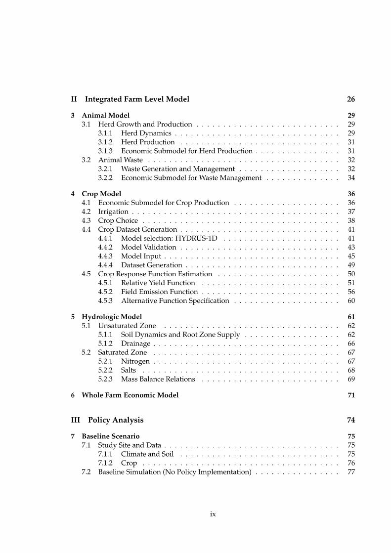
1.1 Average number of cows per dairy in the U.S. and California . . . . . . . . . 4

2.1 Key elements of the integrated farm level model (adapted from Baerenklauet al. [2008]) . . . . . . . . . . . . . . . . . . . . . . . . . . . . . . . . . . . . . 27

3.1 Herd dynamics at a dairy farm . . . . . . . . . . . . . . . . . . . . . . . . . . 31

4.1 Field measured nitrogen uptake vs. simulated nitrogen uptake from Tanji etal. (1979) model & from HYDRUS-1D . . . . . . . . . . . . . . . . . . . . . . 45

4.2 Field measured relative yield vs. simulated relative yield from HYDRUS-1D 464.3 Nitrogen uptake curves for eight small grain forages commonly grown in

California . . . . . . . . . . . . . . . . . . . . . . . . . . . . . . . . . . . . . . . 484.4 Relative yield of the linearized crop vs. relative yield of Swan oat, Longhorn

oat, and Bartali Italian ryegrass . . . . . . . . . . . . . . . . . . . . . . . . . . 484.5 Relative yield vs. available water and available nitrogen when soil salin-

ity is 0, 6, 12, 18, 24, and 30 dS/m. Points: simulated data. Surfaces: fittedfunctions. . . . . . . . . . . . . . . . . . . . . . . . . . . . . . . . . . . . . . . 53

4.6 Polynomial regression of water and nitrogen parameters in the relative yieldfunction . . . . . . . . . . . . . . . . . . . . . . . . . . . . . . . . . . . . . . . 55

4.7 Relative yield function: simulated data vs. fitted data . . . . . . . . . . . . . 564.8 Field emission vs. available water and available nitrogen when soil salin-

ity is 0, 6, 12, 18, 24,and 30 dS/m. Points: simulated data. Surfaces: fittedfunctions. . . . . . . . . . . . . . . . . . . . . . . . . . . . . . . . . . . . . . . 58

4.9 Polynomial regression of water and nitrogen parameters in the field emis-sion function . . . . . . . . . . . . . . . . . . . . . . . . . . . . . . . . . . . . 59

4.10 Field emission function: fitted data vs. simulated data . . . . . . . . . . . . 59

5.1 Conceptual hydrologic model . . . . . . . . . . . . . . . . . . . . . . . . . . . 62

7.1 Baseline: paths of soil organic nitrogen, soil inorganic nitrogen, and soilsalinity for each field type under the optimal activities (flush-lagoon, 1/4-mile furrow, corn-wheat rotation) . . . . . . . . . . . . . . . . . . . . . . . . 80

7.2 Baseline: paths of irrigations under the optimal activities (flush-lagoon, 1/4-mile furrow, corn-wheat rotation), given three sources of irrigation water . . 81

7.3 Baseline: path of fertilizer application under the optimal activities (flush-lagoon, 1/4-mile furrow, corn-wheat rotation), given three sources of fertilizer 82

xi

7.4 Baseline: paths of water infiltration and field emission for each field typeunder the optimal activities (flush-lagoon, 1/4-mile furrow, corn-wheat ro-tation) . . . . . . . . . . . . . . . . . . . . . . . . . . . . . . . . . . . . . . . . . 83

7.5 Baseline: paths of soil inorganic nitrogen, soil salinity, and field emission foreach field type, paths of irrigation and fertilizer application, and seasonalnitrogen emissions under an alternative combination of activities (flush-lagoon, linear move, corn-wheat rotation) . . . . . . . . . . . . . . . . . . . . 86

7.6 Baseline: paths of soil inorganic nitrogen, soil salinity, and field emission foreach field type, paths of irrigation and fertilizer application, and seasonalnitrogen emissions under an alternative combination of activities (scrape-tank, 1/4-mile furrow, corn-wheat rotation) . . . . . . . . . . . . . . . . . . . 87

8.1 Nutrient Management Plans: paths of soil inorganic nitrogen, soil salinity,and field emission for each field type, paths of irrigation and fertilizer appli-cation, and seasonal nitrogen emissions under the optimal activities (scrape-tank, 1/4-mile furrow, corn-wheat rotation) . . . . . . . . . . . . . . . . . . . 92

8.2 Field emission limit: paths of soil inorganic nitrogen, soil salinity, and fieldemission for each field type, paths of irrigation and fertilizer application,and seasonal nitrogen emissions under the optimal activities (flush-lagoon,linear move, corn-wheat rotation) . . . . . . . . . . . . . . . . . . . . . . . . 94

8.3 Downstream emission limit: paths of soil inorganic nitrogen, soil salinity,and field emission for each field type, paths of irrigation and fertilizer appli-cation, and seasonal nitrogen emissions under the optimal activities (flush-lagoon, 1/4-mile furrow, corn-wheat rotation) . . . . . . . . . . . . . . . . . 97

8.4 Downstream emission charge: paths of soil inorganic nitrogen, soil salin-ity, and field emission for each field type, paths of irrigation and fertilizerapplication, and seasonal nitrogen emissions under the optimal activities(flush-lagoon, 1/4-mile furrow, corn-wheat rotation) . . . . . . . . . . . . . 99

xii

List of Tables

4.1 Irrigation System Data . . . . . . . . . . . . . . . . . . . . . . . . . . . . . . . 384.2 Discretization of the log-normal distribution of water infiltration over the field 394.3 HYDRUS-1D specification . . . . . . . . . . . . . . . . . . . . . . . . . . . . . 434.4 Polynomial regression of water and nitrogen parameters in the relative yield

function . . . . . . . . . . . . . . . . . . . . . . . . . . . . . . . . . . . . . . . 564.5 Polynomial regression of water and nitrogen parameters in the field emis-

sion function . . . . . . . . . . . . . . . . . . . . . . . . . . . . . . . . . . . . . 574.6 Scaling factors for calculating relative value . . . . . . . . . . . . . . . . . . . 60

7.1 Model Validation . . . . . . . . . . . . . . . . . . . . . . . . . . . . . . . . . . 797.2 Baseline: irrigation, relative yield, and field emission of nitrogen for each

field type under the optimal activities (flush-lagoon, 1/4-mile furrow, corn-wheat rotation) . . . . . . . . . . . . . . . . . . . . . . . . . . . . . . . . . . . 83

7.3 Baseline : irrigation, relative yield, and field emission for each field typeunder an alternative combination of activities (flush-lagoon, linear move,corn-wheat rotation) . . . . . . . . . . . . . . . . . . . . . . . . . . . . . . . . 84

7.4 Baseline : irrigation, relative yield, and field emission for each field typeunder an alternative combination of activities (scrape-tank, 1/4-mile furrow,corn-wheat rotation) . . . . . . . . . . . . . . . . . . . . . . . . . . . . . . . . 85

9.1 Loss of total net farm income under alternative policy scenarios . . . . . . . 1009.2 Sensitivity analysis on Willingness to Accept Manure (WTAM) . . . . . . . . 1029.3 Sensitivity analysis on the denitrification rate in the unsaturated zone (DR-

UZ) . . . . . . . . . . . . . . . . . . . . . . . . . . . . . . . . . . . . . . . . . . 103

C.1 Corn response function parameters . . . . . . . . . . . . . . . . . . . . . . . . 120C.2 Cotton response function parameters* . . . . . . . . . . . . . . . . . . . . . . 121C.3 Small Grains response function parameters . . . . . . . . . . . . . . . . . . . 122

D.1 Animal Model Parameters . . . . . . . . . . . . . . . . . . . . . . . . . . . . . 124D.2 Crop and Hydrologic Model Parameters . . . . . . . . . . . . . . . . . . . . . 125

xiii

Part I

Introduction

1

Chapter 1

Background

1.1 Animal Feeding Operations

1.1.1 AFOs and CAFOs

The growing world population, together with globally converging diets, has fu-

elled the sustained rise in demand for food of animal origin. Between 1964-66 and 1997-

99, the human population roughly doubled, while the number of domestic animals tripled

[FAO, 2003, Oenema et al., 2005]. During the same period per capita meat consumption

in the developing countries rose by 150 percent and that of dairy products by 60 percent

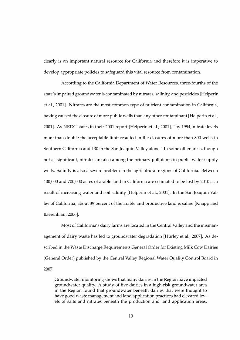
[FAO, 2003]. In the U.S., the national average stocking density for dairy operations in-

creased from 57 to 139 head per farm from 1992 to 2009 [USDA, 2010]. As shown in Figure

1.1, the situation is particularly noticeable in California. California has been the nation’s

leading dairy state since 1993. As of 2009, the average size of a dairy herd in the state

was 1055 cows, much higher than the national average level [CDFA, 2010]. Higher farm

incomes due to economies of scale will sustain the trend toward larger and more concen-

2

trated animal feeding operations, both in developed and rapidly growing economies.

Another significant change throughout the world is land use transformation. For

the U.S. agricultural sector specifically, changes have taken place in cropping patterns with

the total amount of crop land relatively stable [Lubowski et al., 2006]. In California, more

than 1.2 million acres of land for field crops has been converted to vineyards, vegetables,

and orchards in the past three decades [Cooley et al., 2009]. Consolidation combined with

the deceasing acreage for field crops leads to less land available for animal waste disposal,

which is the primary method of disposal. In addition, animal waste (especially dairy and

swine manure) is costly to move relative to its nutrient value. Therefore, the common

practice among operators continues to be over-application of animal waste on land close

to the facility. Excess nutrients from this over-application tend to be transported off the

farm where they can produce adverse environmental and health effects.

In the United States, as of 2003, there are an estimated 1.3 million farms with

livestock, of which 238,000 are considered animal feeding operations [USEPA, 2003]. An

animal feeding operation (AFO) is defined as:

A lot or facility (other than an aquatic animal production facility) where thefollowing conditions are met: (1) Animals have been, are, or will be stabled orconfined and fed or maintained for a total of 45 days or more in any 12-monthperiod, and (2) crops, vegetation, forage growth, or post-harvest residues arenot sustained in the normal growing season over any portion of the lot or facil-ity [USEPA, 2003, Page 7188].

An important category of AFOs is concentrated animal feeding operations (CAFOs) - the

largest of the animal operations and the one that poses the greatest risk to environmental

quality and public health, which are subject to strict environmental regulations. CAFOs

are categorized into a three-tier structure::

3

1992 1994 1996 1998 2000 2002 2004 2006 20080

200

400

600

800

1000

1200

California

U.S.

Year

Num

ber

of

Co

ws

per

Dai

ry

Figure 1.1: Average number of cows per dairy in the U.S. and California

[A]ll large operations are CAFOs, medium operations are CAFOs if they meetspecified risk-of-discharge criteria, and small operations are CAFOs only ifthey are so designated by EPA or the State NPDES permitting authority [USEPA,2003, Page 7189].

The size thresholds for defining Large, Medium, and Small CAFOs in each sector are spec-

ified. Take the dairy sector as an example: a facility confining 700 or more mature dairy

cattle is a Large CAFO, a facility confining 200 to 699 mature dairy cattle is a Medium

CAFO and a facility confining less than 200 mature dairy cattle is a Small CAFO [USEPA,

2003, Table 4.1].

1.1.2 Environmental and Public Health Impacts

In the United States, AFOs annually produce more than 500 million tons of ani-

mal waste[USEPA, 2003]. The composition of waste at a particular operation depends on

the animal species, size, maturity, and animal feed. The main constituents are the same:

nutrients (particularly nitrogen and phosphorus), organic matter, solids, pathogens, and

4

volatile compounds [USEPA, 2003]. When improperly managed, animal waste can pose

substantial risks to public health and ecological systems, as discussed below.

1.1.2.1 Water Pollution

Nutrients Animal waste contains significant quantities of nitrogen and phosphorus. Both

nitrogen and phosphorus have fertilizer value for crop growth, but either can also produce

adverse environmental impacts when it is transported in excess quantities to the environ-

ment. Nutrient pollution is a leading cause of water quality impairment in lakes, rivers,

and estuaries [USEPA, 2000]. Nitrogen and phosphorus accelerate algae production in re-

ceiving aquatic ecosystems and can result in algal blooms, and is associated with a variety

of problems including clogged pipelines, fish kills, and reduced recreational opportunities

[USEPA, 2000].

Besides harming surface water, nitrate-nitrogen reaching groundwater is a po-

tential threat to public health. Two medical conditions have been linked to excessive con-

centration of nitrate in drinking water: methaemoglobinaemia (‘blue-baby syndrome’) in

infants, and stomach cancer in adults [Addiscott, 1996, Bower, 1978]. As of 2000, about

43.5 million people (15 percent of U.S. population) rely on domestic withdraws as their

source of drinking water, primarily from groundwater [Hutson et al., 2004]. These people

are at greater risk of nitrate poisoning than those relying on public water sources, because

the quality and safety of water from domestic wells are not regulated by the Safe Drink-

ing Water Act or, in many cases, by state laws [USEPA, 2003, DeSimone et al., 2009]. In

2009, the National Water-Quality Assessment (NAWQA) Program of the U.S. Geological

Survey published a report that presents a national assessment of water quality in private

5

domestic wells based on samples from about 2,100 wells located in 48 states from 1991

to 2004 [DeSimone et al., 2009]. One of the major reported findings is that nitrate is the

most common contaminant derived from anthropogenic sources that is found at concen-

trations greater than human-health benchmarks. Nitrate occurs naturally in ground water,

but elevated concentrations usually originate from human activities such as fertilizer ap-

plication, animal production, and septic systems [Nolan and Hitt, 2003]. According to the

NAWQA report, concentrations of nitrate are greater than the EPA maximum contaminant

level (MCL) of nitrogen in 4.4 percent of wells throughout the country. The highest con-

centrations of nitrate occur most frequently in aquifers underneath agricultural regions,

such as Central Valley basin-fill aquifers in California and the Basin and Range aquifers in

the Southwest [DeSimone et al., 2009].

Salinity Salinity is a measure of the amount of dissolved salts or ions in the water.

Two typical indexes are used to measure salinity: Total Dissolved Solids (TDS) reported

as mg/L (milligrams per liter) and Electrical Conductivity (EC) reported as dS/m (deci-

Siemens per meter). In this thesis, the EC designation is used.

The salinity of animal waste is directly related to the presence of salts such as

sodium, potassium, calcium, magnesium, chloride, sulfate, bicarbonate, carbonate, and

nitrate, which are from undigested feed that passes unabsorbed through animals [USEPA,

2003]. When animal waste is applied to land, salts build up in the soil and ultimately

accumulate in receiving ecosystems.

Soil salinization is a common problem in areas with low rainfall. High salinity in

the soil can deteriorate soil structure, reduce permeability, restrict plant roots from with-

6

drawing water due to osmotic forces and thus reduce crop yields; when combined with

irrigation and poor drainage, it can lead to permanent soil fertility loss [USEPA, 2003]. Soil

salinity can be maintained at acceptable levels for crop growth by applying excess water

to leach the salts out of soil. However, this management strategy results in excess deep

percolation flows which can create their own set of problems, including the salinization of

the receiving water bodies such as aquifers or streams and rivers. Two strategies have been

proposed to deal with such issues: improvement of irrigation management so that excess

water is not applied over that needed for evapotranspiration and leaching, and reuse of

drainage waters for irrigation of appropriate salt-tolerant crops [Qadir and Oster, 2004].

Salts in water also can have adverse impacts on public health and drinking water

supplies. Even at low levels, salts can increase blood pressure in salt-sensitive individuals,

increasing their risk of stroke and heart attacks [USEPA, 2003]; or if delivered for public

use, even slightly saline water can lead to increased water treatment costs, water loss, and

pipe maintenance [Helperin et al., 2001].

Other Pollutants Animal waste contains other pollutants that can impair estuaries, lakes,

streams and rivers. Organic compounds reaching surface water reduce dissolved oxygen,

which can decrease biodiversity and kill fish. Dissolved solids can lead to surface water

degradation. More than 150 pathogens found in livestock manure pose risks to humans,

including the six human pathogens that account for more than 90 percent of food and

waterborne diseases in humans [USEPA, 2003]. Trace elements, antibiotics, pesticides and

hormones are also potential contaminants contained in animal waste.

7

1.1.2.2 Air Pollution and Greenhouse Gases Emissions

Numerous airborne contaminants (e.g., gases, dust, and microbes) are produced

by or emitted from animal production facilities and their waste disposal practices [Jacob-

son et al., 1999]. Animal housing and manure handling systems generate a variety of

gases1, but only three of them have been studied in detail: hydrogen sulfide, ammonia,

and methane. Hydrogen sulfide poses the largest safety risk in confined spaces, ammo-

nia can result in ecological damage to the environment, and methane contributes to global

warming. Other gases, such as volatile fatty acids and oxides of nitrogen, are currently be-

ing studied in greater detail because of their contribution to odor or their potential impact

on global warming [Jacobson et al., 1999]. Recent studies focus on nitrous oxide (N2O)

offset in crop production for GHG emission reductions in industry sectors by changing

fertilizer management practices [Millar et al., 2010]. As of 2002, AFOs contributed approx-

imately 3 percent of all U.S. nitrous oxide (similar for methane) emissions [USEPA, 2003].

Little information is available on the environmental impact of dust or microbe

emissions. Most research has focused on implications for the indoor air quality affecting

both animals and humans [Jacobson et al., 1999].

1.1.3 California Dairies

California has been the nation’s leading dairy state since 1993 when it surpassed

Wisconsin in milk production. Its 1.84 million dairy cows produced 41.63 billion pounds

of milk in 2011, generating 21.1 percent of the national supply [CDFA, 2012]. Thirty five

1Livestock Buildings can generate up to 168 different compounds, accordnig to O’neill and Phillips [1992].

8

counties contributed to the state’s marketed milk production, of which the top five counties

(Tulare, Merced, Kings, Stanislaus, and Kern) accounted for 71.1 percent of the state’s total

milk production in 2011 [CDFA, 2012]. However, these cows generate over 30 million tons

of manure each year, so proper management of dairy waste on California’s dairy farms is

one of the state’s most pressing environmental issues [USEPA, 2011].

In the 1990s, California’s dairy industry experienced significant growth and con-

centration. In 1993, California’s 4000 dairies produced 2.7 billion gallons of milk; in 1998,

2700 dairies produced 20 percent more milk. During the same time period, the average

number of cows per dairy increased from 367 to 624 [USEPA, 2011]. The trend towards

large farms continues in the new century. The average size of a dairy herd in California

was 656 cows in 2002 and in 2011 it was 1101 cows [CDFA, 2003, 2012]. In the Kern County,

the average number of cows in a dairy operation is up to 3069 [CDFA, 2012]. Increasing

concentration and intensifying production of dairies lead to the concentration of dairy

waste in specific geographic areas, creating a potential threat to California environmental

and public health.

1.1.4 California Groundwater Contamination

California uses more groundwater than does any other state in the nation, ex-

tracting a daily average of 14.5 billion gallons of groundwater [Helperin et al., 2001]. In

2000, approximately 50 percent of California’s population depended on groundwater for

its drinking water supplies [Helperin et al., 2001]. In an average year, groundwater meets

about 25 to 40 percent of California’s urban and agricultural water demands; in drought

years, this percentage can increase to two thirds [Helperin et al., 2001]. Groundwater

9

clearly is an important natural resource for California and therefore it is imperative to

develop appropriate policies to safeguard this vital resource from contamination.

According to the California Department of Water Resources, three-fourths of the

state’s impaired groundwater is contaminated by nitrates, salinity, and pesticides [Helperin

et al., 2001]. Nitrates are the most common type of nutrient contamination in California,

having caused the closure of more public wells than any other contaminant [Helperin et al.,

2001]. As NRDC states in their 2001 report [Helperin et al., 2001], “by 1994, nitrate levels

more than double the acceptable limit resulted in the closures of more than 800 wells in

Southern California and 130 in the San Joaquin Valley alone.” In some other areas, though

not as significant, nitrates are also among the primary pollutants in public water supply

wells. Salinity is also a severe problem in the agricultural regions of California. Between

400,000 and 700,000 acres of arable land in California are estimated to be lost by 2010 as a

result of increasing water and soil salinity [Helperin et al., 2001]. In the San Joaquin Val-

ley of California, about 39 percent of the arable and productive land is saline [Knapp and

Baerenklau, 2006].

Most of California’s dairy farms are located in the Central Valley and the misman-

agement of dairy waste has led to groundwater degradation [Hurley et al., 2007]. As de-

scribed in the Waste Discharge Requirements General Order for Existing Milk Cow Dairies

(General Order) published by the Central Valley Regional Water Quality Control Board in

2007,

Groundwater monitoring shows that many dairies in the Region have impactedgroundwater quality. A study of five dairies in a high-risk groundwater areain the Region found that groundwater beneath dairies that were thought tohave good waste management and land application practices had elevated lev-els of salts and nitrates beneath the production and land application areas.

10

The Central Valley Water Board requested monitoring at 80 dairies with poorwaste management practices in the Tulare Lake Basin. This monitoring hasalso shown groundwater pollution under many of the dairies, including wheregroundwater is as deep as 120 feet and in areas underlain by fine-grained sed-iments [CRWQCB, 2007, pp.6-7].

1.2 Existing Policy Regime

The major Federal environmental law currently affecting animal feeding opera-

tions is the Clean Water Act (CWA). CWA establishes a comprehensive program for pro-

tecting the nation’s waters. Among its core provisions, it prohibits the discharge of pol-

lutants from a point source to waters of the United States except as authorized through a

National Pollutant Discharge Elimination System (NPDES) permit. The Act also requires

EPA to establish national technology-based effluent limitations guidelines and standards

(ELGs) for different categories of sources.

Agriculture has been recognized primarily as a nonpoint pollution source and

exempted from NPDES requirements. Nevertheless, parts of an animal operation, such

as the farmstead (animal production facilities not including the adjacent lands), are easily

identified and more similar to point sources. Therefore, CWA has historically defined the

term ‘‘point source’’ to include CAFOs of more than 1000 animal units (section 502, CWA).

In the mid 1970s, EPA established ELGs and permitting regulations for CAFOs under the

NPDES program [USEPA, 2003]. Similar to traditional point pollution sources in other

industries, CAFOs were required to install acceptable technologies at the site to improve

farmstead structures and control runoff. The exception was the irrigation of wastewater

to crop fields. At that time, the regulations presumed that manure removed from the

11

production area was handled appropriately through land application.

Despite more than three decades of regulation of AFOs, reports of discharge and

runoff of animal waste from these operations persist [USEPA, 2003]. Although this is

in part due to inadequate compliance with and enforcement of existing regulations, the

changes that have occurred in the animal production industries contribute more to the

persisting waste discharge. The continued trend toward fewer but larger operations via

more intensive production methods, coupled with shrinking acreage for hay and pastures,

is concentrating more animal waste within smaller geographic units. A high correlation

has been found between areas with impaired surface and/or ground water due to nutrient

enrichment and areas where dense livestock exist [USEPA, 2003].

In response to these concerns, USDA and EPA announced in 1999 the Unified Na-

tional Strategy for Animal Feeding Operations. The Strategy establishes the goal that “all

AFO owners and operators should develop and implement technically sound, econom-

ically feasible, and site specific comprehensive nutrient management plans (CNMPs) to

minimize impacts on water quality and public health” [USDA and USEPA, 1999, pp.5]. A

comprehensive suite of voluntary programs and regulatory programs are geared to ensure

that AFOs establish appropriate CNMPs for properly managing animal manure, including

on-farm application and off-farm disposal, if any. As specified in the Strategy, voluntary

programs (e.g. locally led conservation, environmental education, and financial assistance,

and technical assistance) address the vast majority of AFOs, while the regulatory program

focuses on high risk operations [USDA and USEPA, 1999].

To approach the goals of the Strategy, EPA published a new rule for CAFOs in

2003. This rule can be seen as a part of the regulatory program proposed by the Strat-

12

egy. It expands the number of CAFOs required to seek NPDES permit coverage up to

15,500 operations, including 11,000 large CAFOs [USEPA, 2003]. One important change is

that the revised ELGs require large CAFOs to prepare and implement site-specific nutrient

management plans (NMPs) for animal waste applied to land. The guidelines for NMPs in-

clude land application rates, setbacks, and other land application Best Management Prac-

tices (BMPs), which are required to be based on the most limiting nutrient for applying

fertilizer to cropland [USEPA, 2003]. NMPs would be nitrogen-based in areas where soil

phosphorus is low and phosphorus-based where soil phosphorus is high [USEPA, 2003].

The nutrient standard can limit animal waste application rates on most land. Without bet-

ter methods for animal waste disposal other than land application, NMPs will increase

competition for land capable of absorbing animal waste and create additional costs for

farm operators.

EPA finalized the rule in 2008 in response to the order issued by the U.S. Court

of Appeals for the Second Circuit in Waterkeeper Alliance et al. v. EPA. There are two

changes relative to the 2003 CAFO regulations. First, only those CAFOs that discharge

or propose to discharge are required to apply for permits; second, CAFOs are required

to submit the NMPs along with their NPDES permits applications, which will then be

reviewed by both permitting authorities and the public [USEPA, 2008]. Nevertheless, the

fundamental restrictions in NMPs remain the same for CAFOs as in the 2003 rule. For a

thorough review of federal and state regulations for water pollution from land application

of animal waste, refer to Centner [2012].

Atmospheric pollutants are regulated under the Clean Air Act (CAA), but CAA

currently does not recognize AFOs for regulatory purposes. Despite the slow progress on

13

regulatory change in practice, air pollution from AFOs is receiving increasing attention in

the academic literature, especially when cross-media effects of some pollutants are taken

into account [Aillery et al., 2005, Baerenklau et al., 2008, Sneeringer, 2009]

1.3 Animal Waste Management

1.3.1 Animal Waste Management Strategies

1.3.1.1 Land Disposal

Nitrogen, phosphate, and potash contents in animal waste represent a potential

substitute for commercial fertilizers on field crops. However, the concentration of CAFOs

in specific regions implies that more facilities are competing for the same amount of land.

Generally, off-site transportation of animal waste over long distances is costly relative to

its nutrient value. Also, cropland operators may be reluctant to receive animal waste from

nearby CAFOs because of the odor and uncertainties (e.g. the amount of nutrient contents,

weeds, and pathogens) associated with the application of the “organic” fertilizer. When

combined, these factors lead to over-application of animal waste on land nearest to the

facility.

In a study of the economics of dairy manure use as fertilizer in Central Texas,

Adhikari et al. [2005] conclude that, at the current costs for loading, hauling, and spread-

ing, dairy manure cannot be economically transported from surplus to deficit areas within

the study area. Their results suggest that off-site land application of dairy manure has

the potential to be profitably substituted for chemical fertilizers, if appropriate subsidies

are paid, either by the government or by dairy operators, or if the moisture content of the

14

manure is reduced.

Paudel et al. [2009] use a GIS-based model to determine the least cost dairy ma-

nure application pattern for Louisiana’s major dairy production area where environmental

quality and crop nutrient requirements are treated as constraints. According to their analy-

sis, the characteristics of dairy manure limit the distribution areas or distances between the

farms and the land over which the manure can be economically spread. Longer distances

between dairies and farmland favor the use of commercial fertilizers on farmland.

1.3.1.2 Wetland Treatment

Wetlands provide a chemical and biological environment suitable for improving

water quality. Constructed wetlands have been used to improve the quality of river wa-

ter, stormwater, coal mine drainage, and municipal sewage [Schaafsma et al., 1999]. The

technology of constructed wetland has been applied and evaluated at dairy farms of rela-

tively small size (less than 200 cows). For large CAFOs, at least to the author’s knowledge,

the potential of wetlands as an alternative treatment for animal waste has neither been

theoretically studied nor empirically investigated.

According to Geary and Moore [1999], a treatment wetland, constructed to re-

duce organic matter and nutrients in dairy parlor waters, does not appear to be suitable as

a treatment option for significantly reducing nutrients in dairy wastewater at a herd size of

110. Schaafsma et al. [1999] discuss a wetland system for treating wastewater from a dairy

farm (170 cows) in Maryland. The analysis of the water samples show that flow through

the wetland system resulted in significant reductions in concentrations of all analytes ex-

cept nitrate/nitrite. Relative to initial concentrations, total nitrogen is reduced 98 percent

15

but nitrate/nitrite increase by 82 percent. One of the possible solutions they propose is re-

circulation of wastewater through the wetland cells to promote denitrification and uptake

of nutrients by plants. The constructed wetland has also been tested on very small animal

farms. Dunne et al. [2005] find that wetland performance is seasonally variable at a 42-cow

organic dairy unit in Ireland with large open space and this variability is primarily con-

trolled by hydrological inputs. MacPhee et al. [2009] adopt a diffused air aeration system

for a constructed wetland receiving dairy wastewater. They concludes that the benefits of

wetland aeration are not great enough to warrant its widespread adoption for small-scale

agricultural systems.

1.3.1.3 Anaerobic Digester System

The waste from dairy and swine operations could support the operation of anaer-

obic digester systems [USEPA, 2003]. Digestion primarily transforms the content of animal

waste to a different form, resulting in small reductions in overall volume [Simpkins, 2005].

Benefits to operators using anaerobic digesters include the cost savings from electricity

generation, control of methane emission, significant odor reduction, and improved mar-

ketability of the digester solids [USEPA, 2003]. However, anaerobic digesters would not

necessarily reduce the nutrients in animal waste. Digesters take available nitrogen and

convert part of it into ammonium in the liquid byproduct, which is more readily available

to plants [USDA, 2007a]. Most of the phosphorus removed from the effluent is concen-

trated in the digested solids [USEPA, 2003]. Through anaerobic digester systems, animal

waste can be made more valuable and less likely to become an odor problem, but remains

subject to land application requirements.

16

Morse et al. [1996] conduct an anaerobic digester survey of California dairy pro-

ducers to investigate the failure of many previously installed methane recovery systems.

Identified problems include poor design, collection of manure in a wet form, and incom-

plete cooperation from electricity companies.

Hurley et al. [2007] focus on clustering of independent dairy operations for gen-

eration of bio-renewable energy. The financial feasibility of regional anaerobic digesters,

which capture methane from dairy manure produced from cows in multiple farms, is em-

pirically analyzed. Their results emphasize the importance of trucking cost as an imped-

iment to centralized digesters under the common flush manure handling system in the

Central Valley. However, as noted in their paper, “As the EPA and regional water control

boards tightens the constraints on how dairy producers dispose of their manure, producers

over time may find that these regulations push them to change their current flush systems

to scrape systems to more efficiently manage the disposal of the manure [Hurley et al.,

2007, pp.vi].” Alternative manure management systems are considered in this thesis as a

potential option that farm operators might take to comply with environmental regulations.

1.3.2 Dairy Manure Management in California

Morse et al. [1996] conduct 139 written and 45 oral surveys to identify practices

for the collection, storage, and use of manure on California dairy farms in Tulare, Fresno,

and Madera counties, where mean milking herd size ranges from 381 to 910 cows. As

presented in their paper,

Liquid wash or flush waters were stored in ponds on 95.9% of the dairies. Set-tling ponds or basins (39.1%) or mechanical solid separators (14.2%) were usedto reduce the solid loading rate in storage ponds. Manure solids were collected

17

by tractors (solid system) or from settling ponds or basins (liquid system). Fewproducers (4.1%) identified composting as a component of manure handling.Liquid manures were used for year-round irrigation (62.2%), spread as slurry(9.5%), sold or transported off the farm (12.2%), or seasonally irrigated (62.2%).Solid manure was spread on farm land (78.4%), used for bedding (27.0%), soldoff the farm (58.1%), removed from the farm (6.8%), or composted (5.4%).

In summary, around 90 percent of the manure from California dairies, liquid and solid, is

applied to land on the farm.

Operators in the Central Valley apparently have chosen flush dairy systems rather

than scrape systems, due to the relatively low cost of water in comparison to labor [Hurley

et al., 2007]. The characteristics of the dairy manure in California, its bulk and relatively

low primary nitrogen, phosphate, and potash levels, generally make it infeasible for most

dairies to participate in a centralized digester or constructed wetland treatment. Land

application remains the most common and most desirable method of utilizing manure at

California’s large dairies.

18

Chapter 2

Literature Review

2.1 Environmental-Economic Analysis for CAFOs

Since EPA published the final rule for CAFOs in 2003, the evaluation of the eco-

nomic impacts for CAFOs to comply with the NMP requirement has received significant

attention in the literature. Ribaudo et al. [2003] evaluate the costs for CAFOs to meet a

nutrient standard at the farm, regional, and national levels. They use a simulation model

developed by Fleming et al. [1998]. The model has two components: the cost of transport-

ing and spreading manure to a specific amount of receiving land, and the benefits from re-

placing commercial fertilizer with manure nutrients. Their farm-level analysis suggested

a 0.5-2.0 percent increase in production costs for large dairies when the willing-to-accept-

manure (WTAM) by surrounding crop producers is 20 percent [Ribaudo et al., 2003]. When

competition for spreadable cropland is introduced in the regional analysis, the costs in-

crease to 40-50 percent of the total net returns, not including the offset associated with the

savings from replacing commercial fertilizers [Ribaudo et al., 2003]. Kaplan et al. [2004]

19

utilize a sector model to evaluate regional adjustments in production and prices when

CAFOs meet nutrient standards. Whether the secondary price effects are sufficient to off-

set the compliance costs depends on crop producers’ WTAM. An unanticipated result in

their study is the increase of nitrogen leaching in some areas due to the expanded crop-

land acres and changes in crop production. Huang et al. [2005] report that 6-17 percent of

medium and large dairy farms in the southwest US would suffer from the NMP require-

ment while other dairies in the region could avoid income loss by leasing additional nearby

cropland at the current cash rent, which may be a tenuous assumption. Two recent studies

use Geographic Information Systems to improve the modeling of spatial transportation of

manure at the regional level [Aillery et al., 2009, Paudel et al., 2009].

Although these studies provide a full perspective on potential economic impacts

for CAFOs to meet nutrient standards, their models are static and fail to reflect changes

in management practices other than spreading manure on additional land and changing

cropping patterns. Baerenklau et al. [2008], arguably the most complete and accurate study

ever performed, implement a structural dynamic whole-farm model, including herd man-

agement, crop production with non-uniform irrigation, waste disposal, and cross-media

effects of nitrogen pollution (via nitrate leaching and ammonia volatilization). The results

indicate the profit losses due to NMP could be much greater than previously anticipated,

even without allowing for regional competition for land. They point out that regulating

leaching rates rather than nitrogen application rates would be more cost-effective. They

also suggest modeling endogenous irrigation system choice, given the observed potential

benefit of more uniform irrigation.

Another set of studies examines alternative policies for animal waste manage-

20

ment at the regional level, triggered by the manure policy intervention in the European

Union. For example, the Dutch Quota System has received substantial attention in litera-

ture [Vukina and Wossink, 2000, Wossink and Gardebroek, 2006, Helming and Reinhard,

2009]. Straeten et al. [2011] use the Flemish policy case to compare a concentration per-

mit trading system with a regular emission permit trading system. The manure spreading

model under the concentration permit is formulated in a framework similar to the classi-

cal warehouse location problem in operation research. The results show better emission

spreading at higher costs under the concentration permit trading system.

2.2 Policy Instruments for Groundwater Protection

The only policy instrument for controlling pollution from CAFOs that has been

discussed in the literature is the NMPs proposed by EPA. However, the problem of over-

application of animal waste to land is a classic agricultural nonpoint source pollution prob-

lem. Therefore, a review of the policies, which have been proposed for the general problem

of nitrogen pollution and salinity from agricultural production, can shed some light on the

appropriate policies for controlling groundwater pollution from CAFOs.

2.2.1 Nitrates in Groundwater

Four types of regulatory targets have been considered to control nitrate pollution

of groundwater in the literature: nitrogen input to the land surface [Berntsen et al., 2003],

direct effluent from the agricultural field/ nitrate leaching from the root zone [Wu et al.,

1994, Helfand and House, 1995, Larson et al., 1996], nitrogen surplus from the agricultural

21

system [Berntsen et al., 2003, Cuttle and Jarvis, 2005], and ambient concentration in the

groundwater aquifer [Almasri, 2007, Peña-Haro et al., 2009]. For each target, two broad

categories of control mechanisms can be implemented: “command and control (CAC)”

(standards and liability rules) or incentive-based instruments (e.g., taxes, subsidies, quo-

tas).

The NMPs established by EPA is an example of the traditional CAC approach.

NMPs require that the land application rates of animal waste must be consistent with

agronomic rates of nutrient uptake by crops. Since NMPs set quantity restrictions upon

the “last-stage” input to the pollution process, it does provide an incentive for farm op-

erators to reduce herd numbers, change feed, or choose different crops to grow on farm.

However, some other management practices (e.g. irrigation methods, wastewater recy-

cling) are overlooked because emissions are not directly regulated, implying potential cost

ineffectiveness of NMPs to reduce groundwater pollution [Baerenklau et al., 2008].

Wu et al. [1994] develop a dynamic model to simulate farmers’ choices (of crops

and irrigation systems) and the resulting levels of farm income and nitrogen runoff/percolation.

Four policies to reduce water pollution are simulated: (a) a tax on nitrogen runoff and per-

colation; (b) a nitrogen use tax; (c) restrictions on irrigation water use; and (d) cost sharing

for adopting modern irrigation technologies. An effluent tax on nitrogen runoff and perco-

lation is shown to be effective in reducing nitrate pollution, while a tax on nitrogen use is

shown to be the least effective policy. The efficacy of the other two policies depends on soil

type. Similarly to [Baerenklau et al., 2008], these results also suggest the NMP requirement

for CAFOs might not be the most cost-effective policy to reduce pollution.

Helfand and House [1995] show that several uniform regulatory instruments can

22

achieve a pollution target at relatively low social cost. Their case study site is the Salinas

Valley of California, where fertilizer applied to lettuce production leads to buildup of ni-

trate in groundwater. Five types of policy instruments are analyzed as different methods

of achieving a 20 percent pollution reduction: (a) separate input taxes for each soil type

and each input (a solution which achieves the social optimum); (b) tax both inputs to pro-

duction, with taxes uniform across soil types; (c) require a uniform percentage rollback in

levels of input use; (d) tax either water or nitrogen uniformly across soil types; and (e)

restrict either water or nitrogen use uniformly across soil types. The socially optimal solu-

tion to (a) is presented only as a benchmark of comparison, which is likely to be infeasible

in practice under heterogeneous conditions. Three of the second-best policies (the water

tax, the policy of identical input taxes for both soil types, and the uniform reduction in all

input use) are nearly as efficient as the use of individual input taxes. Under the uniform

nitrogen tax and the nitrogen use restriction, the welfare loss is the largest relative to the

overall revenues from lettuce production. Larson et al. [1996] later identify water to be the

best single input to tax in this case study.

Fleming and Adams [1997] consider an ambient tax based on groundwater nitrate

concentrations at observation well sites. In the empirical study of irrigated agriculture in

a county of Oregon, the change in farm profitability under a tax that incorporates spatial

differences in physical parameters is compared with that under a uniform tax. The results

indicate that the gains from accounting for spatial variance in physical parameters are

quite modest.

Goetz et al. [2006] bring attention to the distorting effect of intensive margin poli-

cies on the extensive margin. They empirically show that combining a nitrogen input tax

23

with land-use taxes is about 18 percent more cost efficient than a nitrogen input tax alone

and 58 percent more efficient than offsite abatement in the form of groundwater treatment.

2.2.2 Salts in Groundwater

For aquifers beneath irrigated agriculture, three concepts are closely related: ir-

rigation drainage, soil salinity, and groundwater salinity. Unrestricted irrigation drainage

has led to environmental degradation in many areas worldwide, especially in lands such

as California’s San Joaquin Valley. Furthermore, if drainage is improperly controlled, salts

may accumulate in the soil and impact crop productivity.

Soil salinity and drainage generation have a substantially developed literature

in economics [Dinar et al., 1993, Knapp, 1999]. Dinar et al. [1993] evaluated five policy

instruments that have been proposed to address drainage and salinity problems in central

California: (1) surface water tax, (2) drainage tax, (3) surface water quota, (4) drainage

quota, and (5) irrigation technology cost sharing. They show that in general, direct policies

targeting drainage will achieve drainage goals more cost effectively than indirect policies

targeting water use that contributes to drainage.

Scant attention has been paid by economists to groundwater salinization. Knapp

and Baerenklau [2006] provide a brief review. In their paper, a long-term economic-hydrologic

model of agriculturally induced groundwater salinization is implemented to determine ef-

ficient management in the presence of both pumping costs and salt externalities. Pricing

instruments (one for salt emissions and one for groundwater extractions) are set to ensure

the efficient outcome.

24

2.3 Summary

Policy provisions for nitrate and salt pollution in the previous studies take a va-

riety of forms: quotas applied to polluting outputs or contributing inputs; taxes levied

directly on polluting outputs or indirectly on contributing inputs; and public cost shar-

ing for improved input or pollution management technologies. Although these studies

are based on the pollution from crop agriculture, they can provide some insights into the

control of pollution from CAFOs. A tax on nitrogen use and a control on nitrogen applica-

tion have been shown to be the least effective policy [Wu et al., 1994, Helfand and House,

1995], suggesting the nutrient restrictions on CAFOs proposed by EPA are probably not the

appropriate policy to reduce groundwater pollution. Instead, an effluent tax on nitrogen

runoff or a water tax might be more cost-effective.

The fact that regulations on water or irrigation systems can affect nutrient pol-

lution and salinization is not surprising, because water is the media of transport for both

salts and nitrates. For crop agriculture relying upon commercial fertilizers, nutrient pol-

lution and salinization are treated as disparate issues. However, when animal manure

containing both nitrogen and salts is applied to land as organic fertilizer, the two problems

should be addressed simultaneously. As discussed above, except for Baerenklau et al.

[2008], few studies undertake field-level and farm-level analyses of controlling nutrient

emissions from CAFOs. This may be due to the fact that there is very limited informa-

tion on how crop yields and leaching rates respond to varying application rates of water,

nitrogen, and salts.

25

Part II

Integrated Farm Level Model

26

The preceding two chapters present the challenges of controlling groundwater

pollution from CAFOs and of estimating the economic impacts on CAFOs that must com-

ply with environmental regulations. In the following four chapters, I construct an inte-

grated farm level model to address these challenges.

Choice of herd size and

feed management

Choice of manure

handling system

Choice of offsite export of

solid and/or liquid waste

Choice of irrigation

quantity and quality

Choice of irrigation system

Choice of crop

Farm characteristics

at time (t)

Policy

constraints

Amount of waste remaining

for onsite land application

Crop Response Functions

CPF[W, N, S]

Total pollutants

flows at time (t)

Hydrologic

Profit from milk

and culling

Cost of manure handling

Cost of offsite

waste disposal

Cost of irrigation system

Profit from crops

Net farm income

at time (t)

Total amount of waste

Contents of waste

Crop yield

Cost of water use

Field level emission

(Field Emission)

Cost of incentive-

based policies

Farm level emission (Downstream Emission)

Figure 2.1: Key elements of the integrated farm level model (adapted from Baerenklauet al. [2008])

The model is adapted and expanded from the model of Baerenklau et al. [2008].

Following their approach, Figure 2.1 summarizes the key inputs and outputs (bold text),

choice variables (ovals), and sub-components (shaded). Although the model is calibrated

for large dairy farms, it can be easily adapted to other AFOs. The three main building

27

blocks that make up the full model are animal, crop, and hydrological models. The animal

model and the crop model have corresponding economic submodels, which together con-

stitute the whole farm economic model. The hydrological model simulates the pollutant

emission both at the field level and at the farm level. When incentive-based policies are

imposed, the cost of these policies also enters the economic model.

28

Chapter 3

Animal Model

3.1 Herd Growth and Production

The animal model is comprised of a livestock production model coupled with a

herd growth model. The livestock production model calculates the annual output levels

of milk, meat and waste from animal characteristics, such as herd size, herd composition,

feed, and management. The herd growth model traces the livestock population over time,

depending on the calving rate, the mortality rate, the culling rate and the purchasing rate.

3.1.1 Herd Dynamics

Baerenklau et al. [2008] simulate herd dynamics but find it to be not as important

as soil nitrogen dynamics. Following their suggestion, the herd growth component of my

model does not include the formal transition equations for each age cohort. Instead, I only

trace the total number of animals on farm, assuming the structure of the herd is fixed (i.e.,

the numbers of calves, heifers, and milk cows increase or decrease proportionally when

29

the operator buys or sells animals). The herd dynamics are thus simplified by reducing the

number of state variables to one.

The operator works in discrete time and manages the herd. Each year the oper-

ator decides how many animals to retain and how many to cull (or sell), and how many

replacement animals to purchase, if necessary.

A typical cow spends five years on farm: first year as a calf, second year as a

heifer, and the next three years as a milking cow. Assume the herd maintains a fixed

structure (calf : heifer : cow = 12 : 2

5 : 1), as shown in the second column of Figure 3.1.

The herd dynamics are characterized by 1 state variable ht,g (the number of milk cows at

the beginning of year g of time period t)1 and 1 control variable θt,g (the number of milk

cows bought in that year). Figure 3.1 demonstrates how the herd age cohorts evolve over

time. The numbers of calves, heifers, and cows that are culled every year are respectively(12 + 1

10

)ht,g,

115ht,g, and 1

3ht,g. Define a structure vector ζ1 =[12 ,

25 , 1]

and a cull vector

ζ2 =[35 ,

115 ,

13

].

The transition equations of herd areht,g = ht,g−1 + θt,g t = 1, . . . , T, g = 2, . . . , G

ht,1 = ht−1,G + θt,1 t = 1, . . . , T, g = 1

Initial value h0,G is given.

1I adopt three time indices in the model: time period t, year g, and season k. As discussed in Chapter 4,crop rotation is over multiple years. Therefore, I use t to cover a full period of crop rotation. For example, thealfalfa-corn rotation usually takes 6 years. In this case there are 6 years and 12 seasons in one time period. SeeAppendix A for the notations.

30

t t+1 To cull

Calf

Heifer

Cow_age3

Cow_age4

Cow_age5

Figure 3.1: Herd dynamics at a dairy farm

3.1.2 Herd Production

For the production levels of milk and meat, we follow convention and assume

the feed consumption, weight, and milk production is fixed for each age cohort. However,

unlike poultry and swine farms for which both the waste mass (e.g., the amount of nitrogen

in kilograms) and the waste volume (e.g., the amount of wastewater in gallons) per animal

are usually relatively constant, the waste volume generated by a dairy farm significantly

depends on the its management practices, particularly the manure handling system.

Assume each milk cow consumes a fixed group-specific ration that contains five

common components: alfalfa hay, wheat silage, corn grain, soybean meal and protein mix.

Also assume that each cow achieves a group-specific weight and produces a fixed amount

of milk and waste during each lactation.

3.1.3 Economic Submodel for Herd Production

The net profit from herd production is equal to the revenue from milk and meat

production less the total production cost.

31

πherdt =G∑g=1

[pmilkyhht,g − pherd (ζ1θt,g − ζ2ht,g)>

−(f>pfeed + pswf sw

M + pfixh)

(ζ1ht,g)> − pMht,g

]

• πherdt , net profit from herd production in time period t [$/time-period]

• yh, per-cow milk yield [kg/yr]

• ht,g, the number of milking cows at the beginning of year g of time period t

• θt,g, the number of milking cows bought at the beginning of year g of time period t

• ζ1, structure vector

• ζ2, cull vector

• f , 5× 3 matrix for feed consumption [kg/animal/yr]

• f swM , 3×1 vector for water consumption given manure handling systemM [m3/animal/yr]

• pmilk, price of milk [$/kg]

• psw, price of imported surface water [$/m3]

• pM , annualized cost of manure collecting given manure system M [$/cow/yr]

• pherd, 3× 1 vector for prices of selling cohorts [$/animal]

• pfeed, 5× 1 vector for feed price [$/kg]

• pfixh, 3× 1 vector for fixed cost [$/animal/yr]

3.2 Animal Waste

3.2.1 Waste Generation and Management

Animal operations produce waste slurry. Some waste solids are separated and

sold off-site as fertilizer. For the flows of waste nitrogen, refer to Figure A1 in Baeren-

klau et al. [2008]. The remaining liquid waste needs to be disposed, usually in one of

32

the three ways: land application, wetland treatment, or anaerobic digestion [Morse et al.,

1996, Schaafsma et al., 1999, Paudel et al., 2009]. The characteristics of the dairy manure

in California, its bulk and relatively low primary nitrogen and phosphate levels, generally

make it infeasible for most dairies to participate in a centralized digester or a constructed

wetland treatment [Hurley et al., 2007]. Therefore I assume that animal waste is applied to

croplands either on-site or off-site.

Average water use in a dairy is 95-175 gallons per cow per day, depending on how

much water is used to flush manure from the milking parlor and bedding facility [Bray

et al., 2011]. The volume of liquid wastewater is equal to the total water use less water in

milk and evaporative losses from the production system. The characteristics of the waste,

together with the required hauling distance, will determine the volume of waste exported

and the associated cost. An increase in total waste volume will increase the transportation

cost of waste disposal. Following convention, the distance hauled is a function of available

land suitable for spreading animal waste and the willingness to accept manure (WTAM)

of nearby land owners. See Ribaudo et al. [2003] and Baerenklau et al. [2008] for a detailed

discussion.

Two common manure handling systems are considered in the study: flush-lagoon

and scrape-tank. The scrape-tank system is more labor and capital intensive but use much

less water per cow compared to the flush-lagoon system and thus produces a smaller

volume of waste. The two also differ in the method of on-site waste spreading. Under

the flush-lagoon system, wastewater shares the same pipelines with the irrigation system.

Therefore, the non-uniformity of an irrigation system determines the non-uniform land ap-

plication of animal waste. Under the scrape-tank system, waste is transported and spread

33

to land via tractors so presumably it can be uniformly applied over the field2. Currently

the flush-lagoon system is used in about two-thirds of all the California dairies and typi-

cally employed in the Central Valley [Hurley et al., 2007]. The annual total cost of a manure

system equals the annualized fixed cost plus annual operating costs (i.e., power costs and

labor costs) and the cost from non-drinking water consumption. The cost is $47/cow/yr for

flush-lagoon system and $121/cow/yr for scrape-tank system [Bennett et al., 1994], while

the water demand of flush-lagoon system is 241.77m3/cow/yr and that of a scrape-tank

system is 131.24m3/cow/yr [Bray et al., 2011].

3.2.2 Economic Submodel for Waste Management

For waste management, assume revenues can be earned from selling dried solid

waste but excess liquid waste must be transported off-site at the operator’s expense.

πwastet =

G∑g=1

psolsolt,g − L 2g∑

k=2g−1solt,k

−(pbase + pdistr∗t,g

)lt,g − L 2g∑k=2g−1

lt,k

/µM

• πwastet , net profit from waste management in time period t [$/time-period]

• L, the area of cropland on-site [ha]

• solt,g, solid waste nitrogen generated in year g of time period t [kgN/yr]

• solt,k, solid waste nitrogen applied on-site during season k of time period t [kgN/ha]

2In practice, farmers solve an optimization problem to determine the spreading pattern on site since itcosts more to transport waste to further parts of the field. Therefore, tractor spreading is not perfectly uni-form. In such a case, there are two sources of spatial heterogeneity: irrigation and animal waste spreading.New parameters and control variables can be introduced in the future to take into account this “dual spatialheterogeneity”.

34

• lt,g, liquid waste nitrogen generated in year g of time period t [kgN/yr]

• lt,k, liquid waste nitrogen apoplied on-site during season k of time period t [kgN/ha]

• r∗t,g, the average hauling distance in year g of time period t [km] (refer to the appendixof Baerenklau et al. [2008] for details of the waste disposal cost function)

• psol, the price received for dried solid waste [$/kgN]

• pbase, the base price for hauling manure off-site [$/ha-cm]

• pdist, the hauling cost per unit distance [$/ha-cm-km]

• µM , nitrogen concentration of lagoon water given manure system M [kgN/ha-cm]

35

Chapter 4

Crop Model

4.1 Economic Submodel for Crop Production

The net profit from crop production (πcropt ) equals gross returns (crop price times

yield) minus both fixed and variable costs. The fixed production costs (pfixck ) include op-

erating costs such as seed, herbicide, labor, and machinery but not overhead costs. The

variable costs include irrigation and fertilizer costs.

πcropt = L

K∑k=1

J∑j=1

[prβIj p

Rk my

Rk ry

Rt,k,j

]

−pswswt,k − pgwgwt,k − prwrwt,k − p

flflt,k − pfixck

− pIG

prβIj accounts for the non-uniformity of irrigation systems, which are discussed

in Section 4.2. myRk denotes the maximum crop yield in season k given crop rotation R

[Mg/ha], and pRk the coresponding crop price [$/Mg]. ryRt,k,j denotes the relative crop yield

during season k in time period t at field location j given crop rotation R. The relative yield

36

functions are estimated from simulated crop dataset, which are demonstrated in Section

4.4 and 4.5. swt,k, gwt,k, rwt,k, and flt,k are respectively applied surface water [ha-cm/ha],

applied deep groundwater [ha-cm/ha], recycled shallow groundwater [ha-cm/ha], and

applied commercial fertilizer [kgN/ha]. psw and pfl are the prices of imported surface

water [$/ha-cm] and commercial fertilizer [$/kgN], while pgwand prw denote the costs of

pumping groundwater [$/ha-cm]. pI is the annualized cost of an irrigation system given

irrigation system I [$/ha/yr].

4.2 Irrigation

Improved irrigation uniformity has been shown to be a promising method of

cost reduction under environmental regulations. Following Knapp and Schwabe [2008],

the spatial heterogeneity of water distribution over the field is represented by a water

infiltration coefficient β, which has a log-normal distribution with mean E [β] = 1 and

standard deviation SD [β]. Data on common irrigation systems is readily available from

previous studies. SD [β] can be calculated from the Christiansen uniformity coefficient of

each system. See Table 4.1 for irrigation system data and the calculation of SD [β]. All

costs are expressed in 2005 dollars.

To make this model tractable, the log-normal distribution of β is discretized into

three intervals. These intervals can be interpreted as subareas of the field with different

water infiltration coefficients βj , j ∈ 1, 2, 3. I do this in a way such that [β1, β2, β3] =

[0.3, 0.9, 1.7] and characterize the three types of subareas as under-irrigation field, average-

irrigation field, and over-irrigation field. The corresponding probabilities are prβIj , j ∈

37

Table 4.1: Irrigation System Data

IrrigationSystem Type

CapitalCost

[$/ha]

OMCost

[$/ha-yr]

Life[year]

AnnualizedCost

[$/ha-yr]

CUC SD [β]*

1/2-MileFurrow

327 10 5 83.73 70 0.3922

1/4-MileFurrow

428 12 5 108.26 75 0.3226

Linear Move 2571 129 12 403.05 90 0.1259Data source: University of California Committee of Consultants, 1988 [Knapp, 1992]*The standard deviations for β for are computed for each irrigation system such thatCUC = 1−

´∞0 | β − 1 | f (β) dβ.

1, 2, 3. See Table 4.2 for discretized intervals over the field.

4.3 Crop Choice

Typical cropping systems for California dairies consist of sequential winter for-

ages and summer corn rotation. Manure is usually diluted with irrigation water to avoid

applying high concentrations of salts to fields, a practice that would diminish crop yields.

Greater dilution tends to flush more nitrogen into the underlying aquifer. This suggests

that nitrogen-hungry, salt-tolerant crops, as well as more uniform irrigation systems (i.e.,

systems that reduce over-watering parts of a field and thus minimize flushing chemicals

through the soil) could be a promising cost-effective strategy for pollution reduction. The

operator can use either (i) more nitrogen-hungry crops to reduce the amount of nitrogen in

the root zone that is often flushed to groundwater and/or (ii) more salt tolerant crops to re-

duce soil flushing thereby reducing the amount of water that passes through the root zone

and carries nitrogen and salts to groundwater. However, none of the crop response func-

tions in the literature has taken into account the effects of interactions and feedback mech-

38

Table 4.2: Discretization of the log-normal distribution of water infiltration over thefield

IrrigationSystem Type

βIj prβIj

UnderIrrigation

MeanIrrigation

OverIrrigation

UnderIrrigation

MeanIrrigation

OverIrrigation

1/2-MileFurrow

0.13 0.64 0.23

1/4-MileFurrow

0.3 0.9* 1.7 0.08 0.74 0.18

Linear Move 0.00 0.87 0.13* The water infiltration coefficient for mean-irrigation is 0.9 rather than 1 due to loss ofwater along canals, pipelines, etc.

anisms in the whole plant-water-nitrogen-salinity system. The existing functions only ac-

count for and compute partial effects, such as plant-water, plant-water-salinity, and plant-

water-nitrogen [Dinar et al., 1986, Pang et al., 1997, Knapp and Schwabe, 2008]. Therefore,

this study utilizes software developed for simulating water flow and solute transport as

well as root water and nutrient uptake to generate simulated crop datasets, from which

both yield and emission functions are developed. I generate datasets for a subset of crops

which appear to be economically beneficial for the operator, require large amounts of ni-

trogen, and can withstand high salt concentrations.

Several studies incorporate cropping patterns by assuming the farmer chooses

from a set of candidate crops and allocates a proportion of available land to each selected

crop at the beginning of each year, either in linear programming models or in dynamic

frameworks [Wu et al., 1994, Haouari and Azaiez, 2001, Knapp and Baerenklau, 2006].

Linear programming models have also been used to simulate crop rotation [El-Nazer and

McCarl, 1986, Detlefsen, 2004]. The basic concept is that the acreage for a crop next year

should not be larger than the acreage for the previous crop in the sequence. Note that the

39

optimal crop rotation from an agronomic perspective can be different from the optimal

crop rotation from an economic perspective, similar to the case of fisheries management

where the maximum sustainable yield is different from the optimum sustainable yield. An

ideal model would include the dynamics of soil characteristics (i.e., the carry-over of mois-

ture, nitrogen, and salts) and allow the choice of alternative crops at the beginning of each

season. Two recent studies consider crop rotation in a dynamic optimization framework.

Livingston et al. [2008] set up crop choice as a dynamic optimization problem and solve

it over an infinite time horizon. They assume expected crop revenues (also crop yields)

depend on current and the previous year’s crop choices as well as current fertilizer appli-

cations. Under a similar corn-soybean rotation, Cai et al. [2011] examine both one-year and

two-year carry-over effects. In their model, crop yields are assumed to be exogenous with

the yield level responding to current and previous planting decisions. In both studies, the

carry-over effects on crop yields are characterized by a very short history of crop choices,

which are captured in the coefficients of simple regression analyses of experimental crop

yields. The dynamics of soil characteristics and the full effects of carry-over mechanisms

have not been explored in literature.

There are two possible ways of implementing a crop rotation over multiple years:

1) plant the entire farm to a single crop each year, and 2) divide the farm into equal parts,

and rotate the crops within each parcel in such a way that the total acreage of each crop

grown on the farm is about constant each year [Hazell and Norton, 1986]. The latter ap-

proach is the common practice in the real world because it can maximize the utilization of

some machines and equipment, provide continuous feed for animals, and reduce risk by

growing a portfolio of crops rather than a single crop. The former involves fewer state and

40

choice variables and thus would make the whole optimization problem easier to solve.

Over long-term planning horizons, the two approaches are equivalent. Here I model the

crop system following the first approach.

4.4 Crop Dataset Generation

I am not aware of any field experiment with a full set of data on irrigation, soil

nitrogen, nitrogen application rates, soil salinity, crop water uptake, crop nutrient uptake,

crop yield, and nitrate leaching, which is required for estimating the crop response func-

tions. This limited availability of field data is probably due to the high cost of experi-

mentally quantifying the combined effects of multiple input factors on yield and solute

leaching. I thus utilize a computer simulation model to generate the required data, and

use available data to validate the approach.

4.4.1 Model selection: HYDRUS-1D

Several models have been developed to deal with plant growth, water flow, and

solute movement. Pang and Letey [1998] provides a good review. As the authors point

out, none of the existing models is adequate to evaluate the integrated effects of water,

nitrogen, and salinity on crop yield, either because a model does not use the Richard equa-

tion or because a model fails to include one of the effects. They develop a new model,

ENVIRO-GRO, to simulate the effects of irrigation depth, irrigation salinity, and nitrogen

application on plant yield and nitrogen leaching. The simulated results of ENVIRO-GRO

are evaluated against field experiment data, which show good agreements. ENVIRO-GRO

41

might have been an ideal model for the purpose of this study, but the nitrogen component

was removed when ENVIRO-GRO was modified to be a user-friendly version.

HYDRUS-1D software package is a modeling environment for analysis of wa-

ter flow and solute transport in variably saturated porous media [Simunek et al., 2008],

which includes most of the underlying mechanisms in ENVIRO-GRO. In fact, HYDRUS-

1D offers more functioning and flexibility. It is used worldwide and has been shown to be

reliable for modeling water flow and solute transport, especially for processes in soil and

in groundwater. A very recent study [Ramos et al., 2011] evaluates HYDRUS-1D using

data from a field experiment where corn is irrigated with water of varying nitrogen and

salt concentrations. The results show HYDRUS-1D to be a powerful tool for simulating

overall salinity and the concentration of nitrogen species in soil.

Ramos et al. [2011] do not consider the active mechanism of root nutrient uptake,

which is reasonable given their objective to simulate field conditions in a relatively simple

way and give indicative values. Given the objective of quantifying of crop yield and solute

leaching, I utilize the compensated root water and nutrient uptake modules for my study

(through both passive and active mechanisms; see Simunek and Hopmans [2009] for de-

tails). Originally the Active Solute Uptake module in HYDRUS-1D worked with only one

specified solute. However, I need to model the integrated effects of water and two solutes.

I collaborated with the HYDRUS-1D developer (Dr. Jiri Simunek, UC Riverside) to modify

the program such that the module can handle multiple solutes. For modification manual,

see Appendix B. Table 4.3 summarizes the key specifications of my simulation model in

HYDRUS-1D.

42

Table 4.3: HYDRUS-1D specification

Module Specification

Simulated processWater flow, general solute transport, root

water uptake, root growthSoil hydraulic Model van Genuchten-Mualem

Water Flow Boundary ConditionsUpper: atmospheric BC with surface layer.

Lower: free drainage.Solute Transport Equilibrium model

Solute Transport BoundaryConditions

Upper: concentration flux BC. Lower: zeroconcentration gradient.

Root Uptake ModelWater Uptake Reduction Model: Feddes;

Solute Stress Model: multiplicative modelRoot Growth Function 50% after 50% growing season

The outputs of HYDRUS-1D include information on water uptake, solute uptake,

and solute leaching but not on crop yield. External functions are required to relate water

and nutrients uptake to crop yield. Following Pang and Letey [1998], relative yield (ry) is

specified as a function of relative water uptake and relative nitrogen uptake:

ry = min [ryw, ryn] = min

[wupw∗up

,Φ

(nupn∗up

)](4.1)

wup and nup denote the actual amount of water and nitrogen uptake, while w∗up

and n∗up denote the the maximum potential uptake of water and nitrogen. Φ represents

a quadratic relationship [Pang and Letey, 1998, Feng et al., 2005]. Using HYDRUS-1D

output to calculate relative yields from Equation 4.1 gives us full information on crop water

uptake, nitrogen uptake, nitrate leaching, and relative yield.

4.4.2 Model Validation

The best available field experiment data is from a corn trial in Davis, Califor-

nia from 1974 to 1976. The field was treated with 4 different rates of nitrogen fertilizer

43

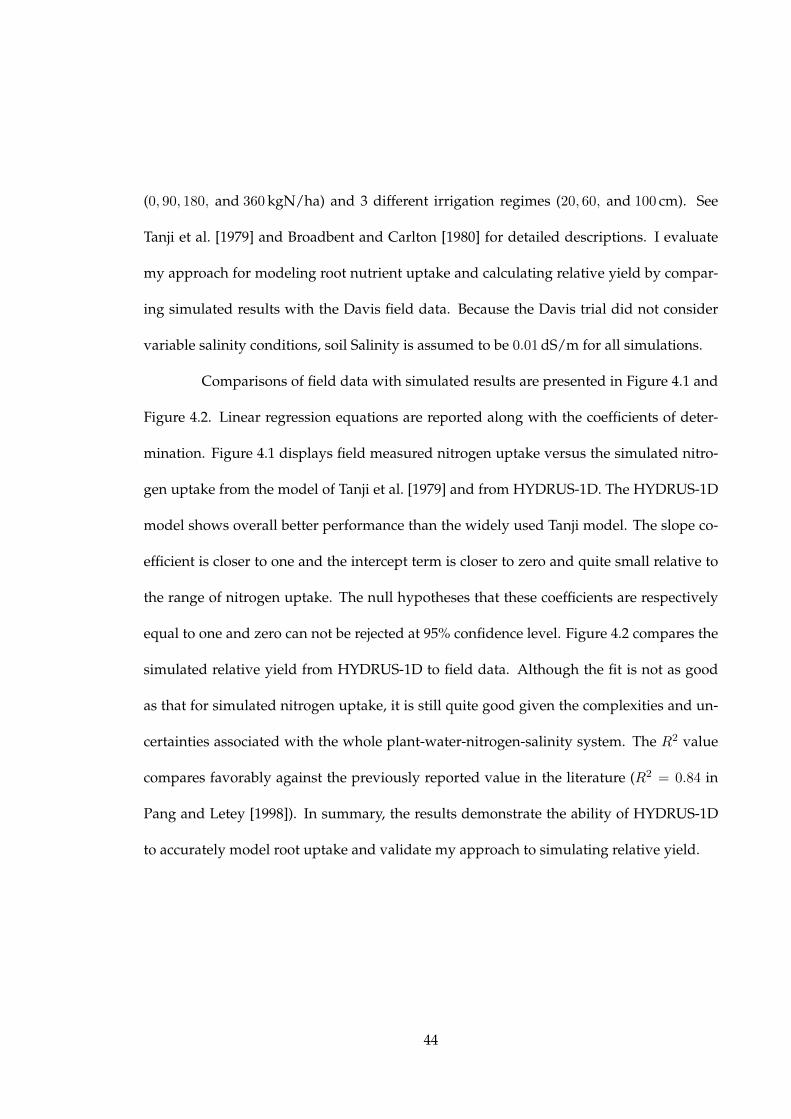
(0, 90, 180, and 360 kgN/ha) and 3 different irrigation regimes (20, 60, and 100 cm). See

Tanji et al. [1979] and Broadbent and Carlton [1980] for detailed descriptions. I evaluate

my approach for modeling root nutrient uptake and calculating relative yield by compar-

ing simulated results with the Davis field data. Because the Davis trial did not consider

variable salinity conditions, soil Salinity is assumed to be 0.01 dS/m for all simulations.

Comparisons of field data with simulated results are presented in Figure 4.1 and

Figure 4.2. Linear regression equations are reported along with the coefficients of deter-

mination. Figure 4.1 displays field measured nitrogen uptake versus the simulated nitro-

gen uptake from the model of Tanji et al. [1979] and from HYDRUS-1D. The HYDRUS-1D

model shows overall better performance than the widely used Tanji model. The slope co-

efficient is closer to one and the intercept term is closer to zero and quite small relative to

the range of nitrogen uptake. The null hypotheses that these coefficients are respectively

equal to one and zero can not be rejected at 95% confidence level. Figure 4.2 compares the

simulated relative yield from HYDRUS-1D to field data. Although the fit is not as good

as that for simulated nitrogen uptake, it is still quite good given the complexities and un-

certainties associated with the whole plant-water-nitrogen-salinity system. The R2 value

compares favorably against the previously reported value in the literature (R2 = 0.84 in

Pang and Letey [1998]). In summary, the results demonstrate the ability of HYDRUS-1D

to accurately model root uptake and validate my approach to simulating relative yield.

44

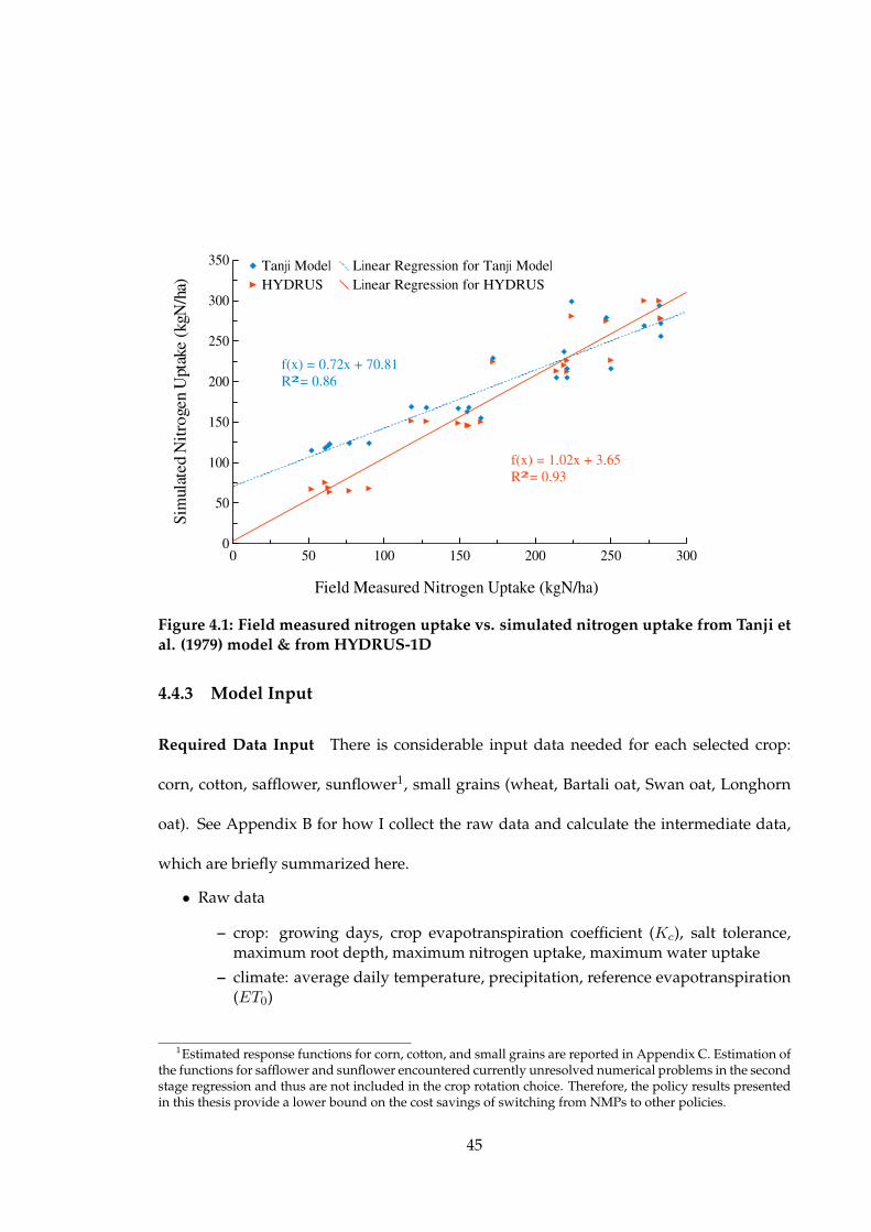
0 50 100 150 200 250 3000

50

100

150

200

250

300

350

f(x) = 1.02x + 3.65

R² = 0.93

f(x) = 0.72x + 70.81

R² = 0.86

Tanji Model Linear Regression for Tanji Model

HYDRUS Linear Regression for HYDRUS

Field Measured Nitrogen Uptake (kgN/ha)

Sim

ula

ted N

itro

gen U

pta

ke (

kgN

/ha)

Figure 4.1: Field measured nitrogen uptake vs. simulated nitrogen uptake from Tanji etal. (1979) model & from HYDRUS-1D

4.4.3 Model Input

Required Data Input There is considerable input data needed for each selected crop:

corn, cotton, safflower, sunflower1, small grains (wheat, Bartali oat, Swan oat, Longhorn

oat). See Appendix B for how I collect the raw data and calculate the intermediate data,

which are briefly summarized here.

• Raw data

– crop: growing days, crop evapotranspiration coefficient (Kc), salt tolerance,maximum root depth, maximum nitrogen uptake, maximum water uptake

– climate: average daily temperature, precipitation, reference evapotranspiration(ET0)

1Estimated response functions for corn, cotton, and small grains are reported in Appendix C. Estimation ofthe functions for safflower and sunflower encountered currently unresolved numerical problems in the secondstage regression and thus are not included in the crop rotation choice. Therefore, the policy results presentedin this thesis provide a lower bound on the cost savings of switching from NMPs to other policies.

45

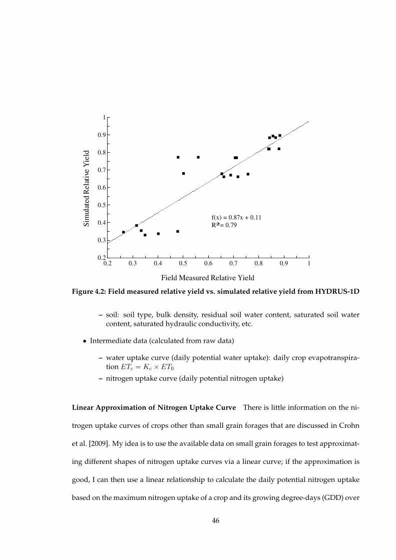
0.2 0.3 0.4 0.5 0.6 0.7 0.8 0.9 10.2

0.3

0.4

0.5

0.6

0.7

0.8

0.9

1

f(x) = 0.87x + 0.11

R² = 0.79

Field Measured Relative Yield

Sim

ula

ted R

ela

tive

Yie

ld

Figure 4.2: Field measured relative yield vs. simulated relative yield from HYDRUS-1D

– soil: soil type, bulk density, residual soil water content, saturated soil watercontent, saturated hydraulic conductivity, etc.

• Intermediate data (calculated from raw data)

– water uptake curve (daily potential water uptake): daily crop evapotranspira-tion ETc = Kc × ET0

– nitrogen uptake curve (daily potential nitrogen uptake)

Linear Approximation of Nitrogen Uptake Curve There is little information on the ni-

trogen uptake curves of crops other than small grain forages that are discussed in Crohn

et al. [2009]. My idea is to use the available data on small grain forages to test approximat-

ing different shapes of nitrogen uptake curves via a linear curve; if the approximation is

good, I can then use a linear relationship to calculate the daily potential nitrogen uptake

based on the maximum nitrogen uptake of a crop and its growing degree-days (GDD) over

46

the season.

Figure 4.3 depicts the nitrogen uptake curves for 8 small grain forages commonly

grown on California dairies. These curves are based on the logistic function developed by

Crohn et al. [2009], where the nitrogen content of a crop is a function of GDD. In practice,

the nitrogen uptake of a crop might be higer than the crop’s nitrogen content, since some

nitrogen can be lost to the atmosphere. Here I assume that the nitrogen uptake and the

nitrogen content of a crop are identical. The curves fall into two categories: sigmoid and

exponential. However, as Crohn et al. [2009] point out, the exponential shapes of two

ryegrass crops are most likely due to forage quality and harvest schedule constraint.

In order to investigate whether the shape of a curve significantly affects actual

nitrogen uptake and relative yield, the simulation results of Swan oat (top curve in Figure

4.3), Longhorn oat (bottom curve in Figure 4.3), and Bartali Italian ryegrass (middle curve

in Figure 4.3) are compared to the simulation results of a linearized version of the crops (the

same crop but with a linear nitrogen uptake curve). All specifications in the HYDRUS-1D

model are exactly same for the four crops except for the daily potential nitrogen uptakes,

which depend on the nitrogen uptake curve.

Figure 4.4 displays the simulation results. The “outliers” are scenarios where

crops receive sufficient water with low salinity but little nitrogen. The t-statistics sug-

gest that the relative yield of the hypothetical crop is statistically equal to relative yield of

Longhorn oat and Bartali Italian ryegrass, and is statistically equal to 98.68% of the relative

yield of Swan oat. I conclude that the effect of the shapes of nitrogen uptake curve is not

statistically significant thereby a linear relationship can be used to approximate nitrogen

uptake curves for my purposes.

47

0 500 1000 1500 2000 25000

50

100

150

200

250

Trical 2700 triticaleSwan oatLonghorn oatEnsiler oatDirkwin wheatCayuse oatBig Daddy ryegrassBartali Italian ryegrass

Time (GDD)

Cro

p N

itrog

en C

onte

nt (

kgN

/ha)

Figure 4.3: Nitrogen uptake curves for eight small grain forages commonly grown inCalifornia

0.0 0.1 0.2 0.3 0.4 0.5 0.6 0.7 0.8 0.9 1.00.0

0.1

0.2

0.3

0.4

0.5

0.6

0.7

0.8

0.9

1.0 Swan oatLonghorn oatBartli Italian ryegrass

Relative Yield of Linearized Crop

Rel

ativ

e Y

ield

Figure 4.4: Relative yield of the linearized crop vs. relative yield of Swan oat, Longhornoat, and Bartali Italian ryegrass

48

4.4.4 Dataset Generation

For each crop, I simulate combinations of at least 5 levels of available water

([0.25, 0.5, 1, 1.5, 2]×w∗up), 5 levels of available inorganic nitrogen ([0.25, 0.5, 1, 1.5, 2]×n∗up),

and 6 levels of soil salinity ([0, 0.2, 0.4, 0.6, 0.8, 1] × EC), which produces at least 150 sce-

narios for each crop. These levels are selected in order to cover most, if not all, of a farm

operator’s possible farming practices even under the hypothetical regulatory scenarios to

be posed later. The highest level of water is double maximum water uptake, taking into

account that the operator might apply excess water to flush salts out of the root zone. The

highest level of nitrogen is also double maximum nitrogen uptake, since animal waste

tends to be over-applied to field at an animal-crop operation.

EC [dS/m] is a critical value of soil salinity at which crop yield decreases to zero.

It is calculated from the salt tolerance parameters of the crop. Maas and Hoffman [1977]

specified the relationship between relative yield and soil salinity as Equation 4.2. When the

soil salinity EC is greater than the threshold value A [dS/m], crop yield starts to decrease.

The slope B expresses yield depression per dS/m. For many crops, both values of A and

B are available in Maas and Hoffman [1977]. Setting relative yield to zero, EC can be

calculated as shown in Equation 4.3.

ry = 1− 0.01B (EC −A) (4.2)

EC = A+100

B(4.3)

49

4.5 Crop Response Function Estimation

In this section, I demonstrate how I use the data presented in the previous section

to fit the crop response functions. These functions provide crop uptakes (of water and

nitrogen, which are required for the mass balance relationships and transition equations

in the whole farm model), crop relative yield, and field emissions of nitrogen to the whole

optimization problem and thus are very useful for policy simulations. Field emissions of

drainage water and salt are calculated according to mass balance relationships in the root

zone, which is demonstrated in Chapter 5.

The crop response functions are expressed as

wup = Ψcwup (w, n, s) (4.4)

nup = Ψcnup (w, n, s) (4.5)

ry = Ψcry (w, n, s) (4.6)

nl = Ψcnl (w, n, s) (4.7)

w, n, and s are respectively crop available water [ha-cm/ha], available inorganic

nitrogen [kgN/ha], and exposed salinity [dS/m]. See Chapter 5 for how to compute the

three input factors during season k in time period t at field location j (i.e., wt,k,j , nt,k,j , and

st,k,j), which need both soil dynamics and mass-balance relationships. wup, nup, ry, and nl

are respectively water uptake [ha-cm/ha], nitrogen uptake [kgN/ha], crop relative yield,

and nitrogen leaching [kgN/ha]. Ψc are functions for crop c that are estimated separately

from the simulated dataset.

The forms of the uptake and relative yield functions are developed from the tra-

ditional Mitscherlich-Baule form. The field emission function is adapted from the nitrate

50

leaching function in Knapp and Schwabe [2008]. Because the estimation methods for the

uptake and relative yield functions are quite similar, I only present the latter in the follow-

ing section. I also take corn as an example to illustrate the logic behind function modifi-

cations and the approximation procedure. Estimation results for the uptake functions of

corn and the response functions of other crops are reported in Appendix C.

4.5.1 Relative Yield Function

Various forms have been proposed for crop yield functions. Griffin et al. [1987]

gives a very good review on twenty traditional and popular functional forms. They also

discuss guidelines for form selection, one of which pertains to application-specific char-

acteristics. Because the resulting functions in this study are to be used in economic op-

timization procedures, continuous differentiability is a desirable property. Llewelyn and

Featherstone [1997] compare five functional forms using corn yield data from the CERES-

Maize simulator for western Kansas. Corn yield is estimated against nitrogen and irriga-

tion water. Their results favor the Mitscherlich-Baule (MB) form over all other specifica-

tions. Also, they show that the costs of incorrectly using the MB form is relatively low.

Shenker et al. [2003] measures the yield response of sweet corn to the combined effects of

nitrogen fertilization and water salinity over a wide range of nitrogen and salinity levels.

Two functional forms are evaluated based on the measured data: Liebig–Sprengel (i.e., lin-

ear von Liebig) and MB. The results suggest that either functional form can successfully

predict water needs, nitrogen needs, and yield. Liebig–Sprengel is a minimization func-

tion derived from von Liebig’s “law of the minimum”. It results in a stepwise response

curve which is not differentiable. Therefore, MB is chosen as the base functional form for

51

relative yield in this study.

The traditional MB function is usually expressed as Equation 4.8, where a repre-

sents a plateau of the production level Y and bi are parameters for the input factorXi. This

function exhibits continuously positive marginal productivities of input factors and allows

for factor substitution. Following this form, relative yield as a function of three inputs can

be written as Equation 4.9. Either absolute yield y or relative yield ry (the ratio of the ac-

tual yield y over the maximum yield y∗) can be the dependent variable, with a equal to y∗

for using absolute yield and a equal to one for relative yield. bw, bn,and bs are respectively

parameters for water, nitrogen, and salinity.

Y = a∏i

(1− exp

(−b1i

(Xi + b0i

)))(4.8)

ry ≡ y

y∗=(1− exp

(−b1w

(w − b0w

))) (1− exp

(−b1n

(n− b0n

)))(1− exp

(−b1s

(s− b0s

)))(4.9)

Unfortunately, Equation 4.9 fails to fit the data well. I find that, given a salinity

level and a nitrogen level, the simulated yields have bell-shaped distributions over the full

range of water levels (Figure 4.5). Therefore, I introduce a parameterized variant of the lo-

gistic probability density function, called the water coefficient ϕ, into the water component

of the function. The logistic distribution is preferred over the normal distribution because

of its heavier tails. Also shown in Figure 4.5, the bell shapes vary for different salinity

levels. Equation 4.9 is thus modified further so that salinity enters the function through its

influence on the water and nitrogen parameters rather than directly as a separate multi-

plicative term.

52

Figure 4.5: Relative yield vs. available water and available nitrogen when soil salinityis 0, 6, 12, 18, 24, and 30 dS/m. Points: simulated data. Surfaces: fitted functions.

53

The relative yield function is thus defined as

ry =(1− exp

(−b1w

(ϕw − b0w

))) (1− exp

(−b1n

(n− b0n

)))(4.10)

where

ϕ =exp (d1w + d0)

4 (1 + exp (d1w + d0))2 + d2

With this specification, each parameter in Υ ≡b1w, b

0w, b

1n, b

0n, d0, d1, d2

is effec-

tively a function of salinity. This approach reduces the computation requirement by break-

ing down the problem into two subproblems.

Subproblem 1 Estimate Equation 4.11 once for each value of s = 0, 6, 12, 18, 24,

30 dS/m, using the appropriate subset of simulated data points.

ry = gry(w, n,Υ) (4.11)

See Equation 4.10 for the explicit form of gry. These estimations produce the

surfaces shown in Figure 4.5. The figures show excellent agreement between simulated

data (points) and fitted data (surfaces) at each salinity level.

Subproblem 2 Estimate each parameter Υi ∈ Υ as a polynomial function of

salinity, as shown in Equation 4.12. Table 4.4 reports the estimated functions and Figure

4.6 depicts the regression curves. Again, agreement between the data (point estimates) and

functions is generally very good.

Υi = f ryi (s) (4.12)

Substitute fitted Equation 4.12 into Equation 4.10 to get relative yield function

Ψry. This approach is verified by the good agreement between simulated data and the

54

5 10 15 20 25 30s HdSmL

0.010

0.012

0.014

0.016

0.018

bw

1

5 10 15 20 25 30s HdSmL

-20

-18

-16

-14

-12

bw

0

5 10 15 20 25 30s HdSmL

0.2

0.4

0.6

0.8

1.0

bn

1

5 10 15 20 25 30s HdSmL

-2.5

-2.0

-1.5

d0

5 10 15 20 25 30s HdSmL

0.08

0.10

0.12

0.14

0.16

0.18

d1

5 10 15 20 25 30s HdSmL

-0.1

0.0

0.1

0.2

0.3

d2

Figure 4.6: Polynomial regression of water and nitrogen parameters in the relative yieldfunction

55

Table 4.4: Polynomial regression of water and nitrogen parameters in the relative yieldfunction

Υi f ryi (s)1 s s2 s3 R2

b1w 0.0181 -7.08E-4 1.48E-5 -6.51E-8 0.9973b0w -10.3161 -0.2408 -0.0270 8.05E-4 0.9815b1n 0.09396 0.2153 -0.0154 2.94E-4 0.7995d0 -2.1708 0.0398 0.0038 -1.84E-4 0.7736d1 0.0627 1.34E-4 -2.62E-5 -5.09E-6 0.9846d2 0.2987 0.0050 -0.0014 2.38E-5 0.9993

fitted relative yield from Ψry (Figure 4.7).

ry = gry(w, n, f ry(s)) = Ψcornry (w, n, s) (4.13)

0 0.1 0.2 0.3 0.4 0.5 0.6 0.7 0.80

0.1

0.2

0.3

0.4

0.5

0.6

0.7

0.8

f(x) = 1.01x − 0

R² = 1

Simulated Relative Yield

Fit

ted R

ela

tive

Yie

ld

Figure 4.7: Relative yield function: simulated data vs. fitted data

4.5.2 Field Emission Function

I test several forms for the field emission (nitrate leaching) function. The function

adapted from Knapp and Schwabe [2008] outperforms the quadratic, cubic, and square

56

root functions, mainly because of its convex-concave behavior and guarantee of a plateau

maximum. In Knapp and Schwabe [2008], nitrogen leaching is specified as a function

of initial soil nitrogen, applied nitrogen, and infiltrated water. Equation 4.14 is a sim-

plified version, where nl is the amount of field emissions [kgN/ha] and n is the total

available nitrogen [kgN/ha]. Similar to the specification of the relative yield function,

ϑ ≡ϑ1w, ϑ

0w, ϑn

are parameters that depend on salinity levels.

nl =ϑn · n

1 + exp (−ϑ1w (w − ϑ0w))(4.14)

ϑi = fnli (s) (4.15)

I adopt the same procedure to estimate the field emission function. Equation

4.14 is estimated for s = 0, 6, 12, 18, 24, 30 dS/m (Figure 4.8). Equation 4.15 is then esti-

mated ∀ϑi ∈ ϑ and substituted into Equation 4.14 to generate the field emission function

Ψnl(w, n, s) (Figure 4.9, Table 4.5). Figure 4.10 shows that the estimated field emission

function fits the simulated data well.

In summary, the results show that my methodologies constitute a reliable ap-

proach to estimating the crop response functions with crop available water, available ni-

trogen, and exposed salinity as three input factors.

Table 4.5: Polynomial regression of water and nitrogen parameters in the field emissionfunction

ϑi fnli (s)1 s s2 R2

ϑ1w 0.4147 -0.0232 0.0004 0.9067ϑ0w 88.1392 0.0046 -0.0087 0.9734ϑn 0.0888 0.0066 -0.0001 0.9878

57

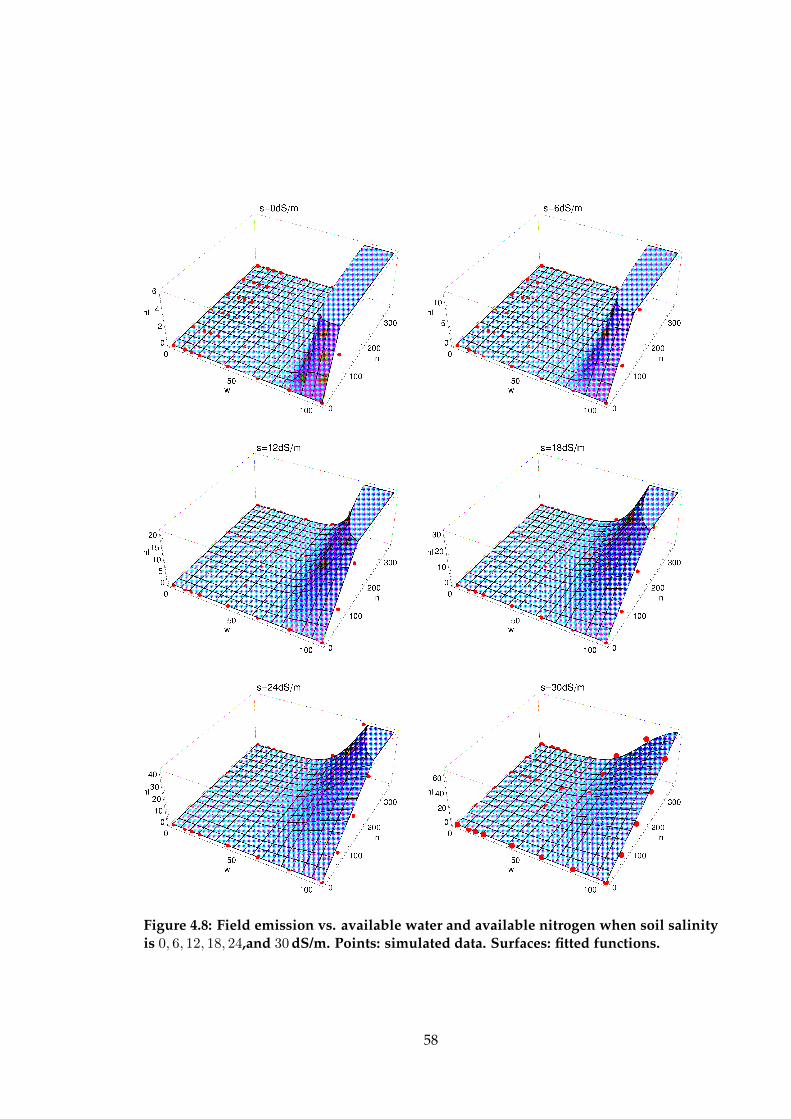
Figure 4.8: Field emission vs. available water and available nitrogen when soil salinityis 0, 6, 12, 18, 24,and 30 dS/m. Points: simulated data. Surfaces: fitted functions.

58

5 10 15 20 25 30s HdSmL

0.1

0.2

0.3

0.4

Jw

1

5 10 15 20 25 30s HdSmL

20

40

60

80

Jw

0

5 10 15 20 25 30s HdSmL

0.05

0.10

0.15

0.20

Jn

Figure 4.9: Polynomial regression of water and nitrogen parameters in the field emissionfunction

0 10 20 30 40 50 60 70 800

10

20

30

40

50

60

70

80

90

f(x) = 1.01x − 0.48

R² = 0.97

Simulated Nitrate Leaching (kgN/ha)

Fit

ted N

itra

te L

eac

hin

g (

kgN

/ha)

Figure 4.10: Field emission function: fitted data vs. simulated data

59

4.5.3 Alternative Function Specification

The crop response functions estimated above depend on absolute values of wa-

ter [cm], nitrogen [kgN/ha], and salinity [dS/m]. As Letey and Dinar [1986] point out,

for purposes of transferring such relationships among different geographical areas, it is

helpful if these functions can be expressed in relative terms. I can achieve this by simple

transformations.

Take the relative yield function as an example. Relative values are equal to abso-

lute values divided by scaling factors, which are listed in Table 4.6. Transform the relative

yield function in Equation 4.13 accordingly to get Equation 4.16, a new function Ω that only

relies on relative terms. Since the scales ET ∗, n∗up, and EC are available for most regions,

Ω can be transferred to the same type of crop grown in different regions.

ry ≡ Gry(w, n, s) ≡ Gry(rw · ET ∗, rn · n∗up, rs · EC

)= Ω

(rw, rn, rs | ET ∗, n∗up, EC

)(4.16)

Table 4.6: Scaling factors for calculating relative value

Absolute Value Scale Relative valueAvailable water w

[cm]Maximum

Evapotranspiration ET ∗

[cm] (or pan evaporation)

rw = wET ∗

Available nitrogenn [kgN/ha]

Maximum nitrogen uptaken∗up [kgN/ha]

rn = nn∗up

Soil salinity s[dS/m]

Salinity critical value EC[dS/m]

rs = sEC

Yield y [ton/ha] Maximum yield y∗ [ton/ha] ry = yy∗

60

Chapter 5

Hydrologic Model

This chapter discusses subsurface flows and biogeochemical processes (i.e., ni-

trates/salts transportation and transformation) in both unsaturated and saturated zones

that are relevant for the model farm. The unsaturated zone produces the three inputs

for the crop response functions and generates field emissions, while the saturated zone

takes the outputs from the unsaturated zone to determine downstream emissions into the

groundwater aquifer.

Figure 5.1 demonstrates my conceptual modeling framework. In addition to pre-

cipitation, the farm operator can obtain water from three sources: surface water (imported

via canals), deep groundwater (old groundwater in the deep aquifer that is not affected

by farm effluent in the short term), and shallow groundwater (drainage water that can be

recycled via capture wells at the downstream end of the farm). The quality and costs of

surface water and deep groundwater are constant. The basic assumption is that, for a sin-

gle farm model, changes of the ground water table and chemical concentrations in the deep

aquifer are neglected. Another way to look at this assumption is a hypothetical aquitard

61

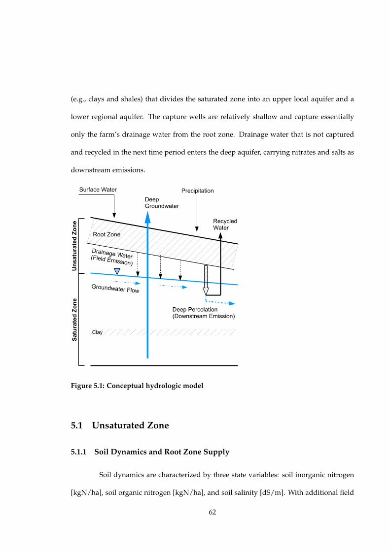
(e.g., clays and shales) that divides the saturated zone into an upper local aquifer and a

lower regional aquifer. The capture wells are relatively shallow and capture essentially

only the farm’s drainage water from the root zone. Drainage water that is not captured

and recycled in the next time period enters the deep aquifer, carrying nitrates and salts as

downstream emissions.

Groundwater Flow

Surface Water

Deep Groundwater

Deep Percolation(Downstream Emission)

Recycled Water

Drainage Water(Field Emission)

Uns

atur

ated

Zon

eSa

tura

ted

Zone

Root Zone

Clay

Precipitation

Figure 5.1: Conceptual hydrologic model

5.1 Unsaturated Zone

5.1.1 Soil Dynamics and Root Zone Supply

Soil dynamics are characterized by three state variables: soil inorganic nitrogen

[kgN/ha], soil organic nitrogen [kgN/ha], and soil salinity [dS/m]. With additional field

62

inputs, the root zone supplies water and chemicals to crops.

Water Equation 5.1 specifies crop available water as the weighted sum of five potenital

sources of water that might be applied to field: surface water (swt,k), deep groundwater

(gwt,k), recycled water (rwt,k), lagoon water (lt,k/µM ), and precipitation (prect,k). Surface

water, deep groundwater, and recycled water are mixed and delivered to the field via the

irrigation system, leading to the spatial heterogeneity of water infiltration (βIj ). Whether

animal waste is uniformly applied depends on the type of manure handling system (βM =

βIj for the flush-lagoon system and βM = 1 for the scrape-tank system). Soil moisture is

relatively low compared to the amount of applied water, and thereby is assumed way

from water available to crops [Letey and Knapp, 1995].

wt,k,j = βIj(swt,k + gwt,k + rwt,k

)+ βM lt,k/µ

M + prect,k (5.1)

Nitrogen Equation 5.2 specifies crop available inorganic nitrogen as a function of soil in-

organic nitrogen (insoilt,k,j), soil organic nitrogen (onsoilt,k,j) , solid (solt,k) and liquid (lt,k) waste

nitrogen applied onsite, total nitrogen from irrigation water (nwt,k,j), the amount of com-

mercial fertilizer applied (flt,k) [kgN/ha], and the rate of atmospheric nitrogen deposition

(adt,k) [kgN/ha]. δk is the seasonal mineralization rate of organic nitrogen, φ is the fraction

of applied liquid waste nitrogen that volatilizes during application, and ω is the fraction

of the organic nitrogen in lagoon water.

nt,k,j = insoilt,k,j + δk

(onsoilt,k,j + solt,k + βMω lt,k

)+ βM (1− φ) (1− ω) lt,k + nwt,k,j + flt,k + adt,k (5.2)

63

The dynamics of soil organic and inorganic nitrogen closely follows Baerenklau

et al. [2008], as shown in Equation 5.3 and 5.4. λk accounts for seasonal denitrification in

the unsaturated zone. Initial values onsoil1,1,j and insoil1,1,j , j = 1, . . . , J , are given.

onsoilt,k+1,j =(1− δk

) (onsoilt,k,j + solt,k + βMω lt,k

),

t = 1, . . . , T ; k = 1, . . . ,K−1; j = 1, . . . , J

onsoilt,1,j =(1− δK

) (onsoilt−1,K,j + solt−1,K + βMω lt−1,K

),

t = 2, . . . , T+1; j = 1, . . . , J

(5.3)

insoilt,k+1,j =(1− λk

)nt,k,j − nupRt,k,j − nlRt,k,j ,

t = 1, . . . , T ; k = 1, . . . ,K−1; j = 1, . . . , J

insoilt,1,j =(1− λK

)nt−1,K,j − nupRt−1,K,j − nlRt−1,K,j ,

t = 2, . . . , T+1; j = 1, . . . , J

(5.4)

In Equation 5.2, the total amount of nitrogen from irrigation water (nwt,k,j) is de-

termined by

nwt,k,j = βIj

(swt,k nc

swt,k + gwt,k nc

gwt,k + rwt,k nc

dwt,k−1

)+ prect,k nc

prect,k ,

t = 1, . . . , T ; k = 2, . . . ,K, j = 1, . . . , J

nwt,1,j = βIj

(swt,1 nc

swt,1 + gwt,1 nc

gwt,1 + rwt,1 nc

dwt−1,K

)+ prect,1 nc

prect,1 ,

t = 1, . . . , T ; j = 1, . . . , J

(5.5)

where ncat,k denote the nitrogen concentration [kgN/ha-cm] of water source a,

a ∈ sw, gw, rw, prec. Set rw1,1 to be zero.

Salt A few models have been developed for predicting salt concentrations in the root

zone under intraseasonal irrigation [Bresler, 1967, Knapp, 1984]. Given my inter-seasonal

modeling framework, I specify a relatively simple model for the dynamics of soil salinity

64

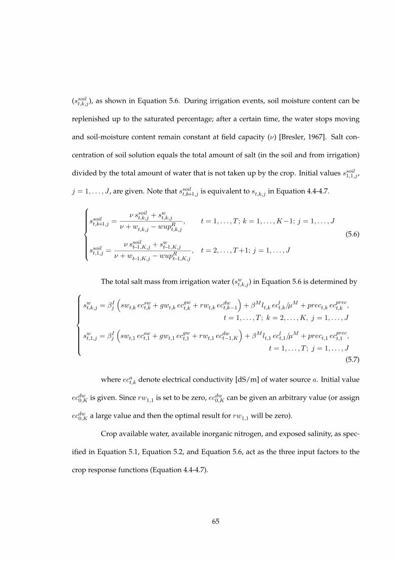
(ssoilt,k,j), as shown in Equation 5.6. During irrigation events, soil moisture content can be

replenished up to the saturated percentage; after a certain time, the water stops moving

and soil-moisture content remain constant at field capacity (ν) [Bresler, 1967]. Salt con-

centration of soil solution equals the total amount of salt (in the soil and from irrigation)

divided by the total amount of water that is not taken up by the crop. Initial values ssoil1,1,j ,

j = 1, . . . , J , are given. Note that ssoilt,k+1,j is equivalent to st,k,j in Equation 4.4-4.7.

ssoilt,k+1,j =

ν ssoilt,k,j + swt,k,j

ν + wt,k,j − wupRt,k,j, t = 1, . . . , T ; k = 1, . . . ,K−1; j = 1, . . . , J

ssoilt,1,j =ν ssoilt−1,K,j + swt−1,K,j

ν + wt−1,K,j − wupRt−1,K,j, t = 2, . . . , T+1; j = 1, . . . , J

(5.6)

The total salt mass from irrigation water (swt,k,j) in Equation 5.6 is determined by

swt,k,j = βIj

(swt,k ec

swt,k + gwt,k ec

gwt,k + rwt,k ec

dwt,k−1

)+ βM lt,k ec

lt,k/µ

M + prect,k ecprect,k ,

t = 1, . . . , T ; k = 2, . . . ,K, j = 1, . . . , J

swt,1,j = βIj

(swt,1 ec

swt,1 + gwt,1 ec

gwt,1 + rwt,1 ec

dwt−1,K

)+ βM lt,1 ec

lt,1/µ

M + prect,1 ecprect,1 ,

t = 1, . . . , T ; j = 1, . . . , J

(5.7)

where ecat,k denote electrical conductivity [dS/m] of water source a. Initial value

ecdw0,K is given. Since rw1,1 is set to be zero, ecdw0,K can be given an arbitrary value (or assign

ecdw0,K a large value and then the optimal result for rw1,1 will be zero).

Crop available water, available inorganic nitrogen, and exposed salinity, as spec-

ified in Equation 5.1, Equation 5.2, and Equation 5.6, act as the three input factors to the

crop response functions (Equation 4.4-4.7).

65

5.1.2 Drainage

Water The volume of water drained from a unit area (dwt,k) [cm/ha] is equal to total

applied water less crop water uptake. Because of non-uniform irrigation systems, the value

is a weighted summation over the J subareas of the field, which is same for all the other

outputs.

dwt,k =

J∑j=1

prβIj (wt,k,j − wupRt,k,j)

Nitrogen Field emission of nitrogen (fent,k) per unit area [kgN/ha] is specified as

fent,k =J∑j=1

prβIj nlRt,k,j

Nitrate concentration of drainage water (ncdwt,k ) [kgN/ha-cm] is then determined

by

ncdwt,k =fent,kdwt,k

Salt Field emission of salt per unit area (fest,k) [cm-dS/m] is specified as

fest,k =

J∑j=1

prβIj dwt,k,j st,k,j

The salinity level of drainage water (ecdwt,k ) [dS/m] is then determined by

ecdwt,k =fest,kdwt,k

The nitrate concentration and the salinity level of drainage water (or recycled

water) enter Equation 5.5 and Equation 5.7 respectively. Drainage water, field emission of

nitrogen, and field emission of salt enter the submodel for the saturated zone.

66

5.2 Saturated Zone

5.2.1 Nitrogen

After the nitrogen leaves the root zone, its transport to the water table is com-

plicated by the various nitrogen species and transformations that can occur in the unsat-

urated zone and saturated zone. The forms and concentrations of nitrogen that reach the

groundwater aquifer are quite site-specific, depending on interactions of physical and mi-

crobial processes such as filtering of particulate organic nitrogen, microbial assimilation,

ammonium sorption, denitrification, and ammonia volatilization [DeSimone and Howes,

1998]. There have been great efforts in the literature trying to quantify the transport and

transformation of nitrogen in groundwater aquifers. From a mass balance analysis, DeSi-

mone and Howes [1998] conclude that ammonification and nitrification in the unsaturated

zone and ammonium sorption in the saturated zone are predominant while loss of fixed

nitrogen through denitrification is minor. Despite these findings in the hydrogeologic and

hydrochemical literatures, all the studies of groundwater nitrogen pollution in the eco-

nomics literature have only accounted for the reactions in root zone and unsaturated zone,

mainly nitrification-denitrification and mineralization of organic nitrogen. Therefore, the

nitrate attenuation capacity of the saturated zone, together with potential cost-saving man-

agement practices, is missing from previous economic analyses of nitrogen pollution of

groundwater.

The processes of ammonification, nitrification, and denitrification in the unsatu-

rated zone are characterized by the parameters φ, δ, andλ in Chapter 5.1.1. For the satu-

rated zone, ammonium sorption and denitrification need to be characterized and incorpo-

67

rated into my model. According to DeSimone and Howes [1998], in the case of a plume

of septage-contaminated groundwater in Massachusetts, ammonium sorption in the satu-

rated zone can remove up to 16 percent of the recharged nitrogen mass from the ground-

water. When applied to the case of land application of dairy manure, adjustments need

to be made depending on field conditions. What is more difficult to determine is whether

and how to account for denitrification in the saturated zone. A closer look at DeSimone

and Howes [1998]’s discussion can be helpful: although denitrification in the anoxic zone

reduced only about 2 percent of the recharged nitrogen mass, they explain that denitrifi-

cation is limited by organic carbon concentrations in the aquifer. Otherwise the nitrogen

mass removed through denitrification will continue to increase, which is indicated by the

expanding anoxic zone in the study site. This coincides with the modeling results of Lee

et al. [2006] for a field study at a cattle feedlot site in Western Australia, where sawdust is

used as an additional carbon source to enhance microbial denitrification. Recently Single-

ton et al. [2007] do find, through their field studies at two dairy operations in the Central

Valley of California, that saturated zone denitrification can mitigate the impact of nitrate

loading at dairy operations, especially when lagoon seepage provides a source of carbon

(local capture wells may intensify this supply by inducing significant lateral flow) and

thus increases the likelihood of denitrification. Although there are many uncertainties,

dairy operations seem to establish conditions conducive to saturated zone denitrification.

5.2.2 Salts

When one thinks about salt in dairy manure, it’s necessary to distinguish between

nutrient salinity and non-nutrient salinity. The major cations in typical irrigation waters

68

are Ca+,Mg2+, and Na+, of which only a small portion are absorbed by plants, while

dairy lagoon waters also have high concentrations of NH+4 and K+that plants can take

up in larger quantities as nutrients [Chang et al., 2005]. If the nutrient part of salinity

(NH+4 and K+) is removed by the crop, it has no impact on crop growth as in typical

salinity case. Analyses of sampled dairy lagoon water in Central Valley of California reveal

that on average the nutrient salinity of the lagoon water is approximately 58 percent of

what the measured EC indicates [Chang et al., 2005].

Salts leaching from the root zone will finally reach groundwater and lead to

groundwater salinization. Through the recycling of wastewater by local pumping, nitro-

gen can be circulated and reused. However, salt is a “conservative” pollutant, which is

not active like nitrogen in soil or groundwater. In the short term, this is not a severe prob-

lem for irrigated agriculture since in some areas saline drainage water is reused and many

studies have demonstrated the feasibility of this management practice [Jury et al., 1978,

Rhoades, 1989, Schwabe et al., 2006]. The long term impacts are still not well understood.

However, due to the high concentration of salts in manure, it’s possible that even a small

amount of recycling water at a dairy operation eventually would turn the location into a

hot-spot of salinity.

5.2.3 Mass Balance Relations

There are various ways to model the groundwater flow and solute transport/

transformation in the saturated zone, such as hydraulic transient models [Harbaugh, 2005]

and concentration response matrices [Peña-Haro et al., 2009]. In this thesis, I take a mass

balance approach.

69

Drainage water that is not recycled enters the aquifer as deep percolation (dpt,k)

[cm/ha]. dpt,k = dwt,k − rwt,k+1, t = 1, . . . , T ; k = 1, . . . ,K − 1

dpt,K = dwt,K − rwt+1,1, t = 1, . . . , T

Downstream emission of nitrogen per unit area (dent,k) [kgN/ha] is specified as

dent,k =

dpt,kdwt,k

fent,k

(1−

(1 +

rwt,k+1

dwt,k

)αdenitr − αmiscel

), t = 1, . . . , T ; k = 1, . . . ,K − 1

dent,K =dpt,Kdwt,K

fent,K

(1−

(1 +

rwt+1,1

dwt,K

)αdenitr − αmiscel

), t = 1, . . . , T

where αdenitr and αmiscel denote the nitrate loss rates due to denitrification and

the other transformation processes. The additional coefficient for αdenitr stands for the

intensified denitrification when more shallow groundwater is pumped.

Downstream emission of salt per unit area (dest,k) [cm-dS/m] is specified as

dest,k =dpt,kdwt,k

fest,k

In this thesis, field emission and downstream emission of nitrogen are the two

main policy targets, for which I simulate and analyze different policy scenarios in Chapter

8.2 and Chapter 8.3. I leave the control of salt emission for future research.

70

Chapter 6

Whole Farm Economic Model

The objective function is specified as

maxθt,g ,lt,k,solt,k,swt,k,gwt,k,rwt,k,f lt,k,M,I,R

[T∑t=1

[ηt(πherdt + πwastet + πcropt − πpolicyt

)]+ ηTpherd (ζ1hT,G)>

](6.1)

subject to transition equations for the state variables, mass balance requirements,

non-negativity constraints, herd permit limits, and policy-related constraints. Net farm in-

come equals the net revenues from herd production, waste disposal, and crop production

less the environmental policy costs (πpolicyt ). η is the discount rate. The last term represents

the salvage value of the herd. All the other variables have been defined previously.

Command-and-control policies enter as constraints to the optimization problem.

Incentive-based policies, which can include surface water tax (χsw), commercial fertilizer

tax (χfl), field nitrogen emission charge (χfe), and downstream nitrogen emission charge

(χde), enter the objective function directly and impose costs on farm production.

71

πpolicyt = L

(χsw

K∑k=1

[pswswt,k

]+ χfl

K∑k=1

[pflflt,k

]+ χfe

K∑k=1

fent,k + χdeK∑k=1

dent,k

)

+ χswG∑g=1

[pswf sw

(ζ1ht,g

)>]The model has 10 state variables: 1 for herd size and 9 for three soil characteristics

(soil organic nitrogen, soil inorganic nitrogen, and soil salinity) across three types of field

subareas. Currently the stochastic nature of parameters such as milk price and crop price

is not included in the model, so rather than set up the problem in a dynamic programming

framework, I treat it in Mathematica as a constrained non-linear programming problem

due to the high dimensionality. The model has three discrete choice variables: manure

handling system M , irrigation system I , and crop rotation R. The choice of manure sys-

tem can be modeled in a similar way to the choice of irrigation system, which is a classical

problem of technology choice. Modeling crop rotation under spatial heterogeneity is a

challenge. The acreage-allocation model is not feasible here, because it is difficult to track

the crops grown at each field type when the acreage for a crop can be freely assigned each

year. This may be why we see in the literature acreage-allocation models with multiple

crops and spatial dynamic models with a single crop but not spatial dynamic models with

multiple crops (or crop rotation). I circumvent the problem by assuming the operator com-

mits to a manure handling system, irrigation system, and crop rotation at the beginning of

the planning horizon without the possibility of switching in the future. At the beginning

of each year in the planning period, the operator decides how many cows to buy or sell

(θt,g), and the amount of liquid animal waste (lt,k), solid animal waste (st,k), surface water

(swt,k), deep groundwater (gwt,k), shallow groundwater (rwt,k) and commercial fertilizers

72

(flt,k) to be applied to the field for each season (k) within that year.

There are two ways to mathematically model discrete variables: 1) mixed integer

programming, and 2) activity analysis. Mixed integer nonlinear programming problems

are difficult to solve, especially for large scale optimization problems. I already have a high

dimensional model with several nonlinearities, so I choose the method of activity analy-

sis. An integral component required for the activity analysis is a “technology-cost” matrix

which describes the inputs and outputs as well as associated costs for each management

practice [Duraiappah, 2003]. In this sense, crop rotation can also be modeled via activ-

ity analysis, since each pattern of crop rotation can be viewed as an alternative farming

technology. I use the KNITRO package to solve the constrained non-linear optimization

problem under alternative activities (i.e., alternative combinations of management prac-

tices), among which the one with the highest net farm income is the optimal solution of

the whole dynamic optimization problem (in the following sections I denote the activities

associated with the optimal solution by “the optimal activities”).

73

Part III

Policy Analysis

74

Chapter 7

Baseline Scenario

7.1 Study Site and Data

7.1.1 Climate and Soil

I collect data on the region of Tulare County and Kern County, which accom-

modate more than 1/3 of the cows in the state. The climate data (temperature, precipita-

tion, pan evaporation) are ten-year averages from 2000-2009 over four CIMIS stations. The

main soil type of farmland in Tulare & Kern is sandy loam/ loamy sand [USDA, 2007b]:

bulk density 1.5 g/cc (range 1.35− 1.70 g/cc), saturated hydraulic conductivity 28µm/sec

(range 14 − 42µm/sec) [USDA, 2009]. According to the soil survey in USDA [2009], the

highest soil salinity in this region is around 20 dS/m, which is well covered by my selected

intervals of soil salinity for the crop response functions.

I assume a discount rate of 4 percent with all economic data inflation-adjusted to

2005 dollars.

75

7.1.2 Crop

Data on production fixed cost and maximum yield is from the University of Cal-

ifornia Cooperative Extension (Cost & Return Studies by UC Davis). Crop prices are from

the National Agricultural Statistics Service.

Fertilizer Commercial fertilizers and noncommercial fertilizers (animal waste) can be ap-

plied to maintain proper nutrition for the crops. Three sources of nitrogen fertilizer in my

model are liquid waste, solid waste, and commercial fertilizer at a cost of $0.59/kgN.

Water Source The farmer can import high quality surface water (EC = 0.15 dS/m and

N = 1 mg/l) with a price of $2.58/ha-cm [Vargas et al., 2003], pump deep groundwater

(EC = 1.18 dS/m and N = 10 mg/l) at a cost of $8.84/ha-cm [Marques et al., 2003], and

pump shallow groundwater through capture wells at a cost of $2.58/ha-cm [Schans, 2001].

The quality of groundwater is updated from GeoTracker GAMA, an online database pro-

vided by the California State Water Resources Control Board.

Surface water prices vary among irrigation districts in the Central Valley. De-

pending on which irrigation district the farm belongs to and the groundwater depth in

that region, the average water cost can range from $1.62/ha-cm to $11.35/ha-cm [Hut-

macher et al., 2003]. Sensitivity analysis on surface water price is performed in Section

9.2.

Irrigation System Initially three types of irrigation systems are considered in this study:

1/2-mile furrow, 1/4-mile furrow, and linear move. According to Baerenklau et al. [2008],

1/2-mile furrow is the common system used by dairy farms in the Central Valley. My

76

preliminary results show 1/2-mile furrow would never be adopted and 1/4-mile furrow

system is the optimal choice under the baseline scenario. Personal communications with

farm advisers in Tulare County (Carol Frate, Oct 21, 2011) suggest that 1/4-mile furrow

system is the most common one in that county, while 1/2-mile furrow is popular in the

northern part of the valley where more surface water is available. Since my empirical

study focuses on the area of Tulare and surrounding counties, I only include 1/4-mile

furrow and linear move system in the simulations and analyses reported here.

My analysis does not consider the scheduling of irrigation and fertilizer appli-

cation. I assume the operator follows the recommended scheduling for a given crop and

irrigation system.

All the parameters of the model are given in Appendix D.

7.2 Baseline Simulation (No Policy Implementation)

I first utilize a sequential solution procedure (using the solution of one single-

period model as the initial values for the subsequent single-period model) to establish a

feasible solution for the dynamic problem, and then use it as the starting point to solve for

the long-term optimal dynamic solution under the baseline scenario.The planning horizon

is 30 years (i.e., 60 seasons). All the simulated scenarios can reach a steady state over the

first 24 years, with boundary effects for some scenarios in the last 6 years (1 time period)1.

Therefore, the following analyses are based on the results of the first 24 years. Table 7.1

1Here I use the term “steady state” in a broader sense than just a terminology associated with infinite de-terministic dynamic programming problems. My model is a finite dynamic problem where the state variablescan achieve steady levels.

77

compares the steady state values of the baseline scenario against available data. Animal

numbers are similar to those in the Hilmar site. As Baerenklau et al. [2008] point out, the

difference in annual profit per cow is due to different assumptions of milk production.

The total net farm income over the years is 26.24 million dollars, which will be used as a

reference value to calculate the relative losses of net farm income under alternative policy

scenarios. The field emission of nitrogen is low compared to that reported in Schans [2001],

which is probably because I assume a deeper root zone of 3 meters. In summary, my model

appears to be calibrated well.

With no environmental regulations in the baseline scenario, the operator opti-

mally selects flush-lagoon as the manure handling system, 1/4-mile furrow as the irriga-

tion system, and corn-wheat as the crop rotation. The herd size remains steady through

time, constrained by the herd permit. Figure 7.1 displays the optimal path of soil organic

nitrogen, soil inorganic nitrogen, and soil salinity, which vary depending on the field type

(i.e., under-irrigation, mean-irrigation, or over-irrigation)2. The optimal decision rule for

seasonal irrigation, as shown in Figure 7.2 , suggests that in order to maintain a certain

level of salinity, the operator periodically applies large volumes of high quality water to

flush the salts out of the soil. This leads to the cyclical patterns in the paths of soil inorganic

nitrogen and soil salinity. We do not see a similar pattern for soil organic nitrogen, since

water is the transporting medium of dissolved salts (including inorganic nitrogen) but not

2For soil inorganic nitrogen, under-irrigation < mean-irrigation < over-irrigation; for soil salinity, under-irrigation > mean-irrigation > over-irrigation. This is because the concentration of inorganic nitrogen is muchhigher than the concentration of salts in animal waste. Meanwhile, the amount of nitrates and salts that canbe carried through the soil is limited during each irrigation and thus during the whole season. Therefore,leaching significantly affects the total amount of salts in soil but not the total amount of inorganic nitrogen.More nitrogen accumulates in the field type which receives more animal waste, and more salts accumulate inthe field type which receives less irrigation water.

78

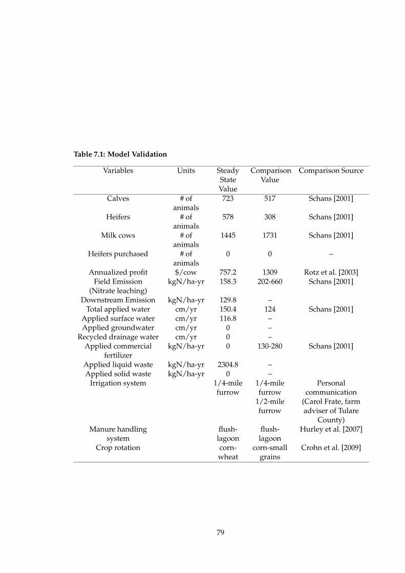
Table 7.1: Model Validation

Variables Units SteadyStateValue

ComparisonValue

Comparison Source

Calves # ofanimals

723 517 Schans [2001]

Heifers # ofanimals

578 308 Schans [2001]

Milk cows # ofanimals

1445 1731 Schans [2001]

Heifers purchased # ofanimals

0 0 –

Annualized profit $/cow 757.2 1309 Rotz et al. [2003]Field Emission

(Nitrate leaching)kgN/ha-yr 158.3 202-660 Schans [2001]

Downstream Emission kgN/ha-yr 129.8 –Total applied water cm/yr 150.4 124 Schans [2001]

Applied surface water cm/yr 116.8 –Applied groundwater cm/yr 0 –

Recycled drainage water cm/yr 0 –Applied commercial

fertilizerkgN/ha-yr 0 130-280 Schans [2001]

Applied liquid waste kgN/ha-yr 2304.8 –Applied solid waste kgN/ha-yr 0 –

Irrigation system 1/4-milefurrow

1/4-milefurrow

1/2-milefurrow

Personalcommunication

(Carol Frate, farmadviser of Tulare

County)Manure handling

systemflush-lagoon

flush-lagoon

Hurley et al. [2007]

Crop rotation corn-wheat

corn-smallgrains

Crohn et al. [2009]

79

0 10 20 30 40 50 600

500

1000

1500

2000

2500

Under−Irrigation Mean−Irrigation Over−Irrigation

t (season)

So

il O

rgan

ic N

itro

gen

(kgN

/ha)

0 10 20 30 40 50 600

500

1000

1500

2000

2500

3000

3500

Under−Irrigation Mean−Irrigation Over−Irrigation

t (season)

So

il I

no

rgan

ic N

itro

gen

(kgN

/ha)

0 10 20 30 40 50 600

5

10

15

20

25

Under−Irrigation Mean−Irrigation Over−Irrigation

t (season)

So

il S

alin

ity

(dS

/m)

Figure 7.1: Baseline: paths of soil organic nitrogen, soil inorganic nitrogen, and soilsalinity for each field type under the optimal activities (flush-lagoon, 1/4-mile furrow,corn-wheat rotation)

80

0 10 20 30 40 50 600

20

40

60

80

100

120

Surface Water Recycled Water Groundwater

Lagoon Water Total Irrigation

t (season)

Wat

er A

ppli

ed (

cm)

Figure 7.2: Baseline: paths of irrigations under the optimal activities (flush-lagoon, 1/4-mile furrow, corn-wheat rotation), given three sources of irrigation water

organic nitrogen.

Figure 7.3 depicts the optimal decision rule for fertilizer application. In the base-

line scenario, the operator does not apply commercial fertilizer or solid waste on site. In

reality, farmers are usually concerned about certain risks associated with manure fertil-

izer, such as pathogens and weeds and the fact that organic nitrogen is not immediately

plant-available. Therefore they also use some commercial fertilizer. This is why we see the

difference between my simulated value and the comparison value for applied fertilizer in

Table 7.1. I do not consider these issues for the dairy operator, but for surrounding land

owners I use three levels of WTAM (20%, 60%, and 100%)3 to account for these concerns

and perform sensitivity analysis in Section 9.2. Furthermore I assume 25% of surrounding

land is suitable for spreading animal waste [Baerenklau et al., 2008].

Figure 7.4 shows the water infiltration and field emission of nitrogen for each field

3All the results presented in this chapter and next chapter are for WTAM equal to 60%.

81

0 10 20 30 40 50 600

200

400

600

800

1000

1200

Liquid WasteSolid WasteCommercial Fertilizer

t (season)

Fer

tili

zer

Appli

ed (

kgN

/ha)

Figure 7.3: Baseline: path of fertilizer application under the optimal activities (flush-lagoon, 1/4-mile furrow, corn-wheat rotation), given three sources of fertilizer

type. Flushing of salt also carries more nitrate from the root zone to groundwater. The

effect is only and especially significant for the mean-irrigated field type. For the under-

irrigated field type, there is no excess water even during flushing. For the over-irrigated

field type, there is enough excess water to carry all leachable nitrate through the soil even

if there is no flushing.

Table 7.2 summarizes the total available water, crop relative yield, and field emis-

sion of nitrogen for each field type over the planning horizon. Although flushing sig-

nificantly increases the leaching for the mean-irrigated subfield, the main contribution of

field emission is from the over-irrigated subfield, due to the high non-uniformity of the

1/4-mile furrow system. The over-irrigated field type makes up 18.28% of the field (Table

4.2), gets 30.83% of total irrigation, produces 19.85% of total crop yield, but accounts for

77.19% of total field emission of nitrogen, which is why Knapp and Schwabe [2008] say

that “nitrogen management is in a very real sense water management.”

To further illustrate the effects of non-uniform irrigation, I report similar infor-

82

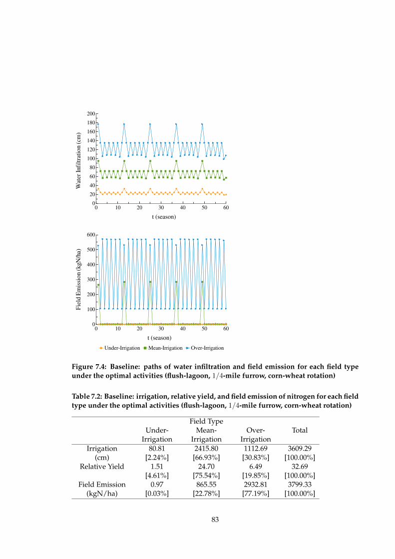
0 10 20 30 40 50 600

20

40

60

80

100

120

140

160

180

200

Under−Irrigation Mean−Irrigation Over−Irrigation

t (season)

Wat

er I

nfi

ltra

tio

n (

cm)

0 10 20 30 40 50 600

100

200

300

400

500

600

Under−Irrigation Mean−Irrigation Over−Irrigation

t (season)

Fie

ld E

mis

sio

n (

kgN

/ha)

Figure 7.4: Baseline: paths of water infiltration and field emission for each field typeunder the optimal activities (flush-lagoon, 1/4-mile furrow, corn-wheat rotation)

Table 7.2: Baseline: irrigation, relative yield, and field emission of nitrogen for each fieldtype under the optimal activities (flush-lagoon, 1/4-mile furrow, corn-wheat rotation)

Field TypeUnder-

IrrigationMean-

IrrigationOver-

IrrigationTotal

Irrigation 80.81 2415.80 1112.69 3609.29(cm) [2.24%] [66.93%] [30.83%] [100.00%]

Relative Yield 1.51 24.70 6.49 32.69[4.61%] [75.54%] [19.85%] [100.00%]

Field Emission 0.97 865.55 2932.81 3799.33(kgN/ha) [0.03%] [22.78%] [77.19%] [100.00%]

83

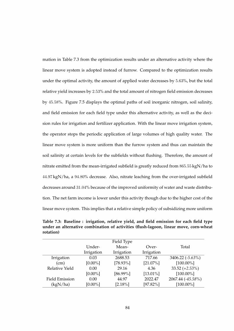
mation in Table 7.3 from the optimization results under an alternative activity where the

linear move system is adopted instead of furrow. Compared to the optimization results

under the optimal activity, the amount of applied water decreases by 5.63%, but the total

relative yield increases by 2.53% and the total amount of nitrogen field emission decreases

by 45.58%. Figure 7.5 displays the optimal paths of soil inorganic nitrogen, soil salinity,

and field emission for each field type under this alternative activity, as well as the deci-

sion rules for irrigation and fertilizer application. With the linear move irrigation system,

the operator stops the periodic application of large volumes of high quality water. The

linear move system is more uniform than the furrow system and thus can maintain the

soil salinity at certain levels for the subfields without flushing. Therefore, the amount of

nitrate emitted from the mean-irrigated subfield is greatly reduced from 865.55 kgN/ha to

44.97 kgN/ha, a 94.80% decrease. Also, nitrate leaching from the over-irrigated subfield

decreases around 31.04% because of the improved uniformity of water and waste distribu-

tion. The net farm income is lower under this activity though due to the higher cost of the

linear move system. This implies that a relative simple policy of subsidizing more uniform

Table 7.3: Baseline : irrigation, relative yield, and field emission for each field typeunder an alternative combination of activities (flush-lagoon, linear move, corn-wheatrotation)

Field TypeUnder-

IrrigationMean-

IrrigationOver-

IrrigationTotal

Irrigation 0.03 2688.53 717.66 3406.22 (-5.63%)(cm) [0.00%] [78.93%] [21.07%] [100.00%]

Relative Yield 0.00 29.16 4.36 33.52 (+2.53%)[0.00%] [86.99%] [13.01%] [100.00%]

Field Emission 0.00 44.97 2022.47 2067.44 (-45.58%)(kgN/ha) [0.00%] [2.18%] [97.82%] [100.00%]

84

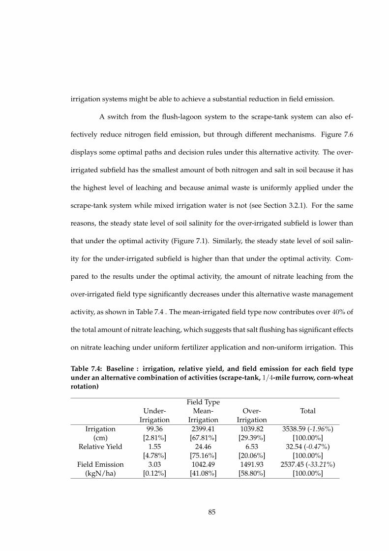
irrigation systems might be able to achieve a substantial reduction in field emission.

A switch from the flush-lagoon system to the scrape-tank system can also ef-

fectively reduce nitrogen field emission, but through different mechanisms. Figure 7.6

displays some optimal paths and decision rules under this alternative activity. The over-

irrigated subfield has the smallest amount of both nitrogen and salt in soil because it has

the highest level of leaching and because animal waste is uniformly applied under the

scrape-tank system while mixed irrigation water is not (see Section 3.2.1). For the same

reasons, the steady state level of soil salinity for the over-irrigated subfield is lower than

that under the optimal activity (Figure 7.1). Similarly, the steady state level of soil salin-

ity for the under-irrigated subfield is higher than that under the optimal activity. Com-

pared to the results under the optimal activity, the amount of nitrate leaching from the

over-irrigated field type significantly decreases under this alternative waste management

activity, as shown in Table 7.4 . The mean-irrigated field type now contributes over 40% of

the total amount of nitrate leaching, which suggests that salt flushing has significant effects

on nitrate leaching under uniform fertilizer application and non-uniform irrigation. This

Table 7.4: Baseline : irrigation, relative yield, and field emission for each field typeunder an alternative combination of activities (scrape-tank, 1/4-mile furrow, corn-wheatrotation)

Field TypeUnder-

IrrigationMean-

IrrigationOver-

IrrigationTotal

Irrigation 99.36 2399.41 1039.82 3538.59 (-1.96%)(cm) [2.81%] [67.81%] [29.39%] [100.00%]

Relative Yield 1.55 24.46 6.53 32.54 (-0.47%)[4.78%] [75.16%] [20.06%] [100.00%]

Field Emission 3.03 1042.49 1491.93 2537.45 (-33.21%)(kgN/ha) [0.12%] [41.08%] [58.80%] [100.00%]

85

0 10 20 30 40 50 600

500

1000

1500

2000

2500

3000

3500

Under−Irrigation Mean−Irrigation Over−Irrigation

t (season)

So

il Ino

rgan

ic N

itro

gen

(kgN

/ha)

0 10 20 30 40 50 600

5

10

15

20

25

Under−Irrigation Mean−Irrigation Over−Irrigation

t (season)

So

il S

alin

ity

(dS

/m)

0 10 20 30 40 50 600

20

40

60

80

100

120

Surface Water Recycled Water Groundwater

Lagoon Water Total Irrigation

t (season)

Wat

er A

ppli

ed (

cm)

0 10 20 30 40 50 600

200

400

600

800

1000

1200

Liquid WasteSolid WasteCommercial Fertilizer

t (season)

Fer

tili

zer

Appli

ed (

kgN

/ha)

0 10 20 30 40 50 600

100

200

300

400

500

600

Under−Irrigation Mean−Irrigation Over−Irrigation

t (season)

Fie

ld E

mis

sion

(kgN

/ha)

0 10 20 30 40 50 600

10

20

30

40

50

60

70

80

90

100

Field Emission Downstream Emission

t (season)

Nit

rogen

Em

issi

on

(kgN

/ha)

Figure 7.5: Baseline: paths of soil inorganic nitrogen, soil salinity, and field emissionfor each field type, paths of irrigation and fertilizer application, and seasonal nitro-gen emissions under an alternative combination of activities (flush-lagoon, linear move,corn-wheat rotation)

86

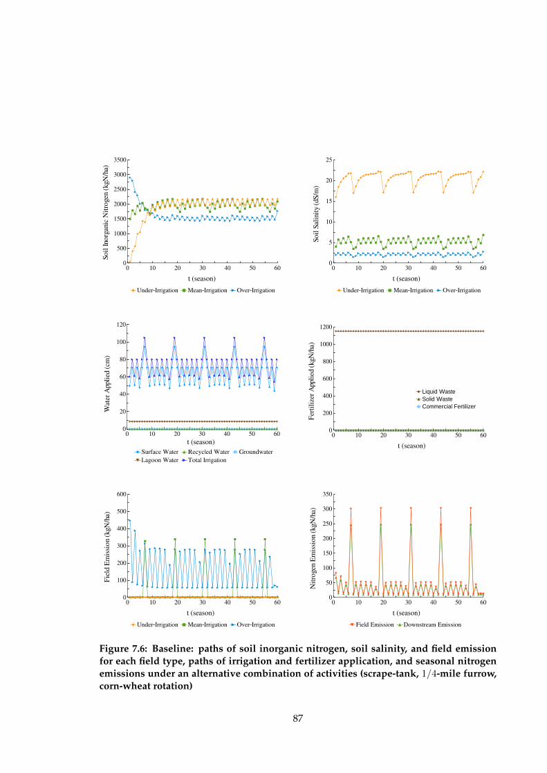
0 10 20 30 40 50 600

500

1000

1500

2000

2500

3000

3500

Under−Irrigation Mean−Irrigation Over−Irrigation

t (season)

So

il Ino

rgan

ic N

itro

gen

(kgN

/ha)

0 10 20 30 40 50 600

5

10

15

20

25

Under−Irrigation Mean−Irrigation Over−Irrigation

t (season)

So

il S

alin

ity

(dS

/m)

0 10 20 30 40 50 600

20

40

60

80

100

120

Surface Water Recycled Water Groundwater

Lagoon Water Total Irrigation

t (season)

Wat

er A

ppli

ed (

cm)

0 10 20 30 40 50 600

200

400

600

800

1000

1200

Liquid WasteSolid WasteCommercial Fertilizer

t (season)

Fer

tili

zer

Appli

ed (

kgN

/ha)

0 10 20 30 40 50 600

100

200

300

400

500

600

Under−Irrigation Mean−Irrigation Over−Irrigation

t (season)

Fie

ld E

mis

sion

(kgN

/ha)

0 10 20 30 40 50 600

50

100

150

200

250

300

350

Field Emission Downstream Emission

t (season)

Nit

rogen

Em

issi

on

(kgN

/ha)

Figure 7.6: Baseline: paths of soil inorganic nitrogen, soil salinity, and field emissionfor each field type, paths of irrigation and fertilizer application, and seasonal nitrogenemissions under an alternative combination of activities (scrape-tank, 1/4-mile furrow,corn-wheat rotation)

87

is also of great importance to crop agriculture, where commercial fertilizers are usually

uniformly applied but water infiltrations varies spatially. For the whole field, the amount

of applied water, the total relative yield, and the total amount of field emission decreases

by 1.96%, 0.47% and 33.21% respectively, compared to the results under the optimal activ-

ity. Again, the net farm income is lower under this activity due to the higher cost of the

scrape-tank system, but a policy that subsidizes water-saving manure collecting systems

and/or more uniform waste distribution systems might also be able to achieve a substan-

tial reduction in field emission.

88

Chapter 8

Alternative Policy Scenarios

Five alternative policy scenarios are simulated and analyzed in this thesis: NMPs,

field emission limit (FEL), field emission charge (FEC), downstream emission limit (DEL),

and downstream emission charge (DEC). NMPs is a quantity restriction on a contributing

input. FEL and FEC are, respectively, a quantity restriction and emission charge on the

intermediate pollution (i.e., the amount of pollutants emitted at an intermediate stage of

their transport and transformation), while DEL and DEC are, respectively, a quantity re-

striction and emission charge on the final pollution (i.e., the net amount of pollutants that

actually leave the property and enter the ecosystem). Therefore, the five policies span three

levels of policy target and two types of control mechanism.

I am interested in the “life cycle” of a pollutant (i.e., different levels of pollution)

because policies targeting the final pollution can be more cost-effective. The intuition is

that these policies can create incentives for polluters to take into account more potential

compliance strategies than policies that target inputs or intermediate pollutant emissions.

This approach is similar to the widely used method of Life-Cycle Assessment in the sense

89

that Life-Cycle Assessment tracks a commercial product while my analysis tracks a pol-

lutant, both of which can help avoid a narrow outlook on environmental and economic

concerns. Ideally, I need to link a physical-chemical-biological model with the evolution in

space and time of the pollutant to an economic model. The whole farm model discussed

in Part II is an attempt to achieve this goal.

The policy simulations are designed to evaluate the cost-effectiveness of alter-

native policies compared to NMPs: I use the field and downstream emissions from the

optimal solutions under NMPs as reference points. To wit, I adjust the emission limits

and charges under the FEL and FEC so that they achieve the same level of field emissions

as achieved under the optimal NMPs; similarly, I adjust the emission limits and charges

under the DEL and DEC to achieve the same downstream level of nitrogen loadings as

achieved by the optimal solutions under NMPs1. The losses of net farm income are then

compared. For each policy simulation, I assume the operation is initially at the steady

state derived from the baseline scenario and then solve for the dynamically optimal prac-

tices under that policy.

8.1 Nutrient Management Plans

According to CRWQCB [2007], potential nitrogen sources available for each crop

should at least include “manure, process wastewater, irrigation water, commercial fertiliz-

ers, soil, and previous crops”. In my model, manure and process wastewater are equiva-

1Therefore, the field emissions from the optimal solutions under NMPs, FEL, and FEC are same, and thedownstream emissions from the optimal solutions under NMPs, FEL, and FEC, DEL, and DEC are same.

90

lent to the animal waste, and nitrogen from previous crops is captured by soil dynamics. It

is noted that the General Order requires soil tests from the land application area only once

every 5 years for soluble phosphorus [CRWQCB, 2007]. Therefore, soil nitrogen is not ac-

counted for by NMPs. As specified in Equation 8.1, the NMP requirement is included in

the model as a constraint on seasonal application of inorganic nitrogen, which is the total

of the nitrogen from applied animal waste (inorganic nitrogen plus the amount of organic

nitrogen that is mineralized during that season), fertilizers, and irrigation water.

(1− ω) lt,k + δk(solt,k + ω lt,k

)+ flt,k + nwt,k ≤ 1.4nR∗up (8.1)

Results show that the operator optimally selects scrape-tank as the manure han-

dling system, 1/4-mile furrow as the irrigation system, and corn-wheat as the crop rotation

under the NMPs scenario. The main results are displayed in Figure 8.1 . Due to the NMP

constraint, the operator hauls almost half of the liquid waste off site. This results in sig-

nificant decreases in soil organic nitrogen, soil inorganic nitrogen, and soil salinity levels

of the mean-irrigated and over-irrigated subfields, even compared to the baseline results

under the same activity (Figure 7.6). Another change in the management practices is the

irrigation pattern. Although the total amount of surface water applied over the planning

horizon increases little, the water is smoothly applied without flushing. That is why the

soil salinity of the under-irrigated subfield remains high. Compared to the baseline sce-

nario under its optimal activities, both the field emission and the downstream emission of

nitrogen decrease by 84.10%. Total crop revenue increases by 6.24% but the operator still

suffers a heavy net income loss of 27.40%, primarily due to the high cost of offsite waste

hauling.

91

0 10 20 30 40 50 600

500

1000

1500

2000

2500

3000

3500

Under−Irrigation Mean−Irrigation Over−Irrigation

t (season)

So

il Ino

rgan

ic N

itro

gen

(kgN

/ha)

0 10 20 30 40 50 600

5

10

15

20

25

Under−Irrigation Mean−Irrigation Over−Irrigation

t (season)

So

il S

alin

ity

(dS

/m)

0 10 20 30 40 50 600

20

40

60

80

100

120

Surface Water Recycled Water Groundwater

Lagoon Water Total Irrigation

t (season)

Wat

er A

ppli

ed (

cm)

0 10 20 30 40 50 600

200

400

600

800

1000

1200

Liquid WasteSolid WasteCommercial Fertilizer

t (season)

Fer

tili

zer

Appli

ed (

kgN

/ha)

0 10 20 30 40 50 600

100

200

300

400

500

600

Under−Irrigation Mean−Irrigation Over−Irrigation

t (season)

Fie

ld E

mis

sion

(kgN

/ha)

0 10 20 30 40 50 600

10

20

30

40

50

60

70

80

90

100

Field Emission Downstream Emission

t (season)

Nit

rogen

Em

issi

on

(kgN

/ha)

Figure 8.1: Nutrient Management Plans: paths of soil inorganic nitrogen, soil salinity,and field emission for each field type, paths of irrigation and fertilizer application, andseasonal nitrogen emissions under the optimal activities (scrape-tank, 1/4-mile furrow,corn-wheat rotation)

92

8.2 Field Emission Control

8.2.1 Field Emission Limit

The total amount of field emissions over the 24 years horizon is 604.2 kgN/ha, or

approximately 25.2 kgN/ha per year, which is set as the annual cap on field emissions2.

The optimal activities under the FEL scenario are flush-lagoon as the manure

handling system, linear move as the irrigation system, and corn-wheat as the crop rota-

tion. Figure 8.2 displays the main results. Unlike under the NMPs scenario, the operator

does not transport any liquid waste off site with a field emission limit. Instead, the oper-

ator controls the rate of field emission by applying less irrigation water and thus holding

a large pool of nitrogen in the soil. The first term on the right-hand side of Equation 5.4

indicates that denitrification in the unsaturated zone can transform the total available in-

organic nitrogen into nitrogen gas at a rate of λk, which is a fixed parameter in the model.

If more inorganic nitrogen remains in the soil over the season, more becomes nitrogen gas

and less nitrate is leached. Therefore, rather than allows nitrate and salt to leach down

to the aquifer, the operator takes advantage of the natural processes to reduce the field

emissions of nitrogen.

The reduction in irrigation mainly happens in summer, since the winter crop is

more salt-tolerant and under the baseline scenario field emissions from the summer crop-

ping is five times more than that from the winter cropping (Figure 7.5). Less irrigation

2I also test a 6-year cap of 151.05kgN/ha for field emission. The optimal solution is similar to that underthe annual cap, with the net farm profit slightly higher due to the added flexibility provided by this longertime horizon. In practice, an emissions limit or charge would be imposed on estimated (or modeled) nitrogenemissions.

93

0 10 20 30 40 50 600

500

1000

1500

2000

2500

3000

3500

4000

4500

Under−Irrigation Mean−Irrigation Over−Irrigation

t (season)

So

il Ino

rgan

ic N

itro

gen

(kgN

/ha)

0 10 20 30 40 50 600

5

10

15

20

25

30

Under−Irrigation Mean−Irrigation Over−Irrigation

t (season)

So

il S

alin

ity

(dS

/m)

0 10 20 30 40 50 600

20

40

60

80

100

120

Surface Water Recycled Water Groundwater

Lagoon Water Total Irrigation

t (season)

Wat

er A

ppli

ed (

cm)

0 10 20 30 40 50 600

200

400

600

800

1000

1200

Liquid WasteSolid WasteCommercial Fertilizer

t (season)

Fer

tili

zer

Appli

ed (

kgN

/ha)

0 10 20 30 40 50 600

100

200

300

400

500

600

Under−Irrigation Mean−Irrigation Over−Irrigation

t (season)

Fie

ld E

mis

sion

(kgN

/ha)

0 10 20 30 40 50 600

10

20

30

40

50

60

70

80

90

100

Field Emission Downstream Emission

t (season)

Nit

rogen

Em

issi

on

(kgN

/ha)

Figure 8.2: Field emission limit: paths of soil inorganic nitrogen, soil salinity, and fieldemission for each field type, paths of irrigation and fertilizer application, and seasonalnitrogen emissions under the optimal activities (flush-lagoon, linear move, corn-wheatrotation)

94

leads to higher levels of soil salinity in the subfields, which can reduce the crop yields.

Compared to the optimal results of the baseline scenario, net farm income decreases by

only 0.79%, with 7.20% of the crop revenue sacrificed to meet the field emission standard.

This implies that quantity control of intermediate pollution is much more cost-effective

than quantity control of polluting inputs for the case of nitrogen emissions. The reasons

are twofold: First, there is limited information on the relationships between the multiple

inputs and the pollution, so it is difficult to determine the best approach of regulating the

inputs (e.g., which one/ones to regulate and how to). Secondly, and what is more impor-

tant, the field emission limit creates incentives for the operator to examine the contribution

of other management practices to pollution in addition to land application of waste, such

as the choice of irrigation system and the pattern/rates of irrigation, which can affect the

natural attenuation of nitrogen.

8.2.2 Field Emission Charge

A per-unit effluent charge can be applied to field emissions. For each combina-

tion of activities, I derive the field emission charge that would produce the same amount

of field emissions as NMPs and FEL. A lump-sum return of emission charge does not alter

marginal conditions so the optimal activity of FEC (or DEC) when the charge revenue is

returned to the industry is same as that when the charge revenue is not returned. At an

emission charge of $2.5/kgN/ha, the operator achieves the same level of emission reduc-

tion at a net income loss of 0.79% (emission charge is not counted as production cost under

the assumption that it would be returned as a lump-sum). The optimal activity and other

management practices are the same as that under the field emission limit.

95

8.3 Downstream Emission Control

8.3.1 Downstream Emission Limit

The total amount of downstream emissions over the 24 years horizon is 495.4

kgN/ha, or approximately 20.6 kgN/ha per year, which is set as the annual cap on down-

stream emissions.

The optimal activities under the downstream emission limit scenario are the same

as those under the baseline scenario. As shown in Figure 8.3 , the most dramatic change

in the management practices is that the operator starts to recycle the drainage water of

low quality with less surface water imported. As a result, salt accumulates in the soil more

quickly so the operator periodically applies a high volume of surface water to flush the salt

out of the field. Similar to the FEL scenario, the operator controls the downstream emis-

sions by taking advantage of natural processes rather than transporting liquid waste off

site. However, the mechanisms under DEL and FEL are different, since the field emissions

from the optimal solution under DEL (117.47 kgN/ha per year) are very high relative to

that under FEL (25.2 kgN/ha per year). The onsite recycling of drainage water has two

effects: (1) crops reuse some of the nitrate so that the amount of nitrate that deep percola-

tion carries into the deep aquifer will decrease, and (2) pumping of shallow groundwater

(i.e., drainage water) intensifies the process of denitrification in the saturated zone so that

more nitrogen enters the atmosphere as nitrogen gas rather than enters the deep aquifer

as nitrate pollution. I test the significance of each of the two effects by running the model

under DEL with and without the second effect; the results suggest that the second effect is

the main driving force of the overall effects introduced by recycling drainage water.

96

0 10 20 30 40 50 600

500

1000

1500

2000

2500

3000

3500

4000

Under−Irrigation Mean−Irrigation Over−Irrigation

t (season)

So

il Ino

rgan

ic N

itro

gen

(kgN

/ha)

0 10 20 30 40 50 600

5

10

15

20

25

30

Under−Irrigation Mean−Irrigation Over−Irrigation

t (season)

So

il S

alin

ity

(dS

/m)

0 10 20 30 40 50 600

20

40

60

80

100

120

Surface Water Recycled Water Groundwater

Lagoon Water Total Irrigation

t (season)

Wat

er A

ppli

ed (

cm)

0 10 20 30 40 50 600

200

400

600

800

1000

1200

Liquid WasteSolid WasteCommercial Fertilizer

t (season)

Fer

tili

zer

Appli

ed (

kgN

/ha)

0 10 20 30 40 50 600

100

200

300

400

500

600

700

Under−Irrigation Mean−Irrigation Over−Irrigation

t (season)

Fie

ld E

mis

sion

(kgN

/ha)

0 10 20 30 40 50 600

20

40

60

80

100

120

Field Emission Downstream Emission

t (season)

Nit

rogen

Em

issi

on

(kgN

/ha)

Figure 8.3: Downstream emission limit: paths of soil inorganic nitrogen, soil salinity,and field emission for each field type, paths of irrigation and fertilizer application, andseasonal nitrogen emissions under the optimal activities (flush-lagoon, 1/4-mile furrow,corn-wheat rotation)

97

Compared to the optimal results of the baseline scenario, net farm income de-

creases by only 0.74%, with 6.73% of the crop revenue sacrificed to meet the downstream

emission standard. This implies that for the case of farm nitrogen emission, quantity con-

trol of the final pollution is more cost-effective than quantity control of the intermediate

pollution. The arguments for controlling inputs versus controlling intermediate pollution

also applies here. The downstream emission limit creates an incentive for the operator to

examine the potential benefits of recycling drainage water, which come from the natural

attenuation capacity of the saturated zone.

8.3.2 Downstream Emission Charge

Similar to FEC, I derive the downstream emission charge that would produce

the same amount of downstream emission as NMPs, FEL, FEC, and DEL. At an emission

charge of $2.04/kgN/ha, the operator achieves the same level of downstream emission re-

duction at a net income loss of 0.70% (emission charge is not counted as production cost).

The optimal activity are same as and the management practices are close to those under

DEL (Figure 8.4 ). Compared to the optimal results of DEL, the 0.04% extra savings in

compliance costs are made possible by allowing occasional flexible levels of nitrate leach-

ing over the planning horizon. This sheds lights on the advantages of emission charge over

direct quantity control when seasonal or annual emissions are heterogeneous either due to

inherent operation practices (e.g., different seasonal crops in rotation) or the accumulation

of precursors to the pollution (e.g., accumulation of soil inorganic nitrogen).

98

0 10 20 30 40 50 600

500

1000

1500

2000

2500

3000

3500

4000

Under−Irrigation Mean−Irrigation Over−Irrigation

t (season)

So

il Ino

rgan

ic N

itro

gen

(kgN

/ha)

0 10 20 30 40 50 600

5

10

15

20

25

30

Under−Irrigation Mean−Irrigation Over−Irrigation

t (season)

So

il S

alin

ity

(dS

/m)

0 10 20 30 40 50 600

20

40

60

80

100

120

Surface Water Recycled Water Groundwater

Lagoon Water Total Irrigation

t (season)

Wat

er A

ppli

ed (

cm)

0 10 20 30 40 50 600

200

400

600

800

1000

1200

Liquid WasteSolid WasteCommercial Fertilizer

t (season)

Fer

tili

zer

Appli

ed (

kgN

/ha)

0 10 20 30 40 50 600

100

200

300

400

500

600

700

Under−Irrigation Mean−Irrigation Over−Irrigation

t (season)

Fie

ld E

mis

sion

(kgN

/ha)

0 10 20 30 40 50 600

20

40

60

80

100

120

Field Emission Downstream Emission

t (season)

Nit

rogen

Em

issi

on

(kgN

/ha)

Figure 8.4: Downstream emission charge: paths of soil inorganic nitrogen, soil salinity,and field emission for each field type, paths of irrigation and fertilizer application, andseasonal nitrogen emissions under the optimal activities (flush-lagoon, 1/4-mile furrow,corn-wheat rotation)

99

Chapter 9

Results and Discussions

9.1 Policy Simulation Results

Table 9.1 summarizes the policy simulation results under four sets of combined

activities. For each policy, the optimal combination of activities is the one with the lowest

loss of net farm income, which then is the loss of net farm income under that policy. The

optimal combination of activities for NMPs, FEL, FEC, DEL, and DEC are respectively A3,

A2, A2, A1, and A1, and the losses of net farm income are respectively 27.40%, 0.79%,

Table 9.1: Loss of total net farm income under alternative policy scenarios

A1 A2 A3 A4*

NMPs 34.90% 35.00% 27.40% 27.83%FEL 1.99% 0.79% 8.88% 9.45%FEC† 3.42% 1.61% 9.00% 9.54%FEC 0.72% 0.79% 8.88% 9.45%DEL 0.74% 0.79% 8.88% 9.45%DEC† 1.00% 1.27% 9.00% 9.54%DEC 0.70% 0.79% 8.88% 9.45%

* A1: flush-lagoon, 1/4-mile furrow; A2: flush-lagoon, linear move; A3: scrape-tank, 1/4-mile furrow; A4: scrape-tank, linear move.† No lump-sum return of emission charge

100

0.79%, 0.74%, and 0.70%. The policies targeting downstream emission are slightly more

cost-effective than the policies targeting field emission, but all of them are much more

cost-effetive than NMPs which targets nitrogen input.

Incentive-based mechanisms are slightly more cost-effective than quantity con-

trols. The field emission charge is an interesting case. From the regulator’s perspective, the

most cost-effective outcome under FEC is a net income loss of 0.72%, which is lower than

that under FEL. However, this outcome is attainable only when there is a single farm oper-

ation or when all the operations are homogeneous given the following sequences of action:

the operators move first by adopting a combination of activities, then the regulator sets the

charge rate accordingly, and then the charge revenue is lump-sum returned. Amacher and

Malik [1998] deveop a theoretical model to compare outcomes with an emission tax and an

emission standard in a cooperative bargaining framework. One of the implications from

their model is that the regulator might not be able to achieve the first-best outcome if it

moves first. When firms face discrete technologies, emission tax payments can create a

divergence between the firms’s technology preferences and that of the regulator [Amacher

and Malik, 1998]. My empirical results back up their theory.

According to the results in Table 9.1, the activity A4 is dominated by A3. Also,

the optimal results of quantity control and emission charge, either for field emission or for

downstream emission, are very close. Therefore, for sensitivity analysis in next section, I

only include NMPs, FEL, and DEL under A1, A2, and A3.

101

9.2 Sensitivity Analysis

9.2.1 Willingness to Accept Manure

Table 9.2 presents the results of sensitivity analysis on WTAM of surrounding

land owners1. As they are less willing to accept manure from CAFOs, the costs for the

dairy operation to meet emission targets under all the policy scenarios increase. However,

the cost of complying with NMPs is most sensitive to WTAM. When WTAM decreases

from 60% to 20%, the cost of NMPs increases from 27.4% to 32.74% while that of DEL from

0.74% only to 0.79%. The reason is obvious given the discussions in Chapter 8: under FEL

or DEL, the operator controls nitrogen emission by taking advantage of natural processes

rather than transporting half of the liquid waste off site, the cost of which largely depends

on WTAM. With lower WTAM, FEL and DEL are more favorable to NMPs.

Table 9.2: Sensitivity analysis on Willingness to Accept Manure (WTAM)

WTAM Policy NPV loss(%)

FieldEmission

DownstreamEmission

A1 A2 A3 (kgN/ha/yr) (kgN/ha/yr)Baseline 0.00% 158.31 129.81

100% NMPs 32.16% 32.26% 25.79% 25.59 20.99FEL 1.30% 0.78% 8.88% 25.59 20.99DEL 0.73% 0.78% 8.88% 134.45 20.99

Baseline 0.00% 158.31 129.8160% NMPs 34.90% 35.00% 27.40% 25.17 20.64

FEL 1.99% 0.79% 8.88% 25.17 20.64DEL 0.74% 0.79% 8.88% 117.47 20.64

Baseline 0.00% 158.76 130.1820% NMPs 38.59% 38.69% 32.74% 23.58 19.34

FEL 5.14% 0.83% 8.89% 23.58 19.34DEL 0.79% 0.83% 8.89% 134.65 19.34

1If a parameter changes, the initial values for the baseline scenario and its steady states usually also change.Therefore, I report relative values rather than absolute ones.

102

9.2.2 Denitrification Rate

The two main natural processes that the operator takes advantage of are denitri-

fication in the unsaturated and saturated zone. Table 9.3 reports the results of sensitivity

analysis on the denitrification rate in the unsaturated zone. Under the baseline scenario,

the nitrogen emissions significantly decrease as the denitrification rate increases, suggest-

ing that denitrification in the unsaturated zone is an important process. Also, as the den-

itrification rate increases, the decrease in nitrogen emissions under NMPs brings stricter

emission regulations and thus higher net income losses. Compared to NMPs, the costs of

complying with FEL and DEL are more sensitive to the denitrification rate in the unsat-

urated zone, since denitrification only matters for nitrogen that is already applied to the

field.

Table 9.3: Sensitivity analysis on the denitrification rate in the unsaturated zone (DR-UZ)

DR-UZ Policy NPV loss(%)

FieldEmission

DownstreamEmission

A1 A2 A3 (kgN/ha/yr) (kgN/ha/yr)Baseline 0.00% 358.74 294.17

0.125 NMPs 34.71% 34.91% 27.31% 43.49 35.66FEL 5.89% 0.70% 8.79% 43.49 35.66DEL 0.62% 0.70% 8.79% 198.64 35.66

Baseline 0.00% 158.31 129.810.25 NMPs 34.90% 35.00% 27.40% 25.17 20.64

FEL 1.99% 0.79% 8.88% 25.17 20.64DEL 0.74% 0.79% 8.88% 117.47 20.64

Baseline 0.00% 91.70 75.190.375 NMPs 35.12% 35.04% 27.44% 17.74 14.55

FEL 0.82% 0.83% 8.93% 17.74 14.55DEL 0.79% 0.83% 8.93% 84.62 14.55

A change of denitrification rate in the saturated zone will affect the results un-

103

der DEL but not those under FEL. Therefore, the conclusion that FEL (and DEL) is much

more cost-effective than NMPs will hold for different levels of denitrification rate in the

saturated zone2.

9.3 Conclusions

This thesis uses an integrated farm level model to empirically evaluate alterna-

tive policy mechanisms for pollution control at the field and the farm level. The optimized

characteristics of the animal-crop operation are consistent with available data. Optimal

decision rules from the optimization problem demonstrate best management practices,

some of which are overlooked in previous studies [Ribaudo et al., 2003, Huang et al., 2005,

Baerenklau et al., 2008], for CAFOs to improve their economic and environmental per-

formance. Novel crop response functions are derived from simulated data to account for

the effects of interactions and feedback mechanisms in the whole plant-water-nitrogen-

salinity system. The spatial heterogeneity of water and nitrogen application over the field,

combined with the integrated effects of water, nitrogen, and salinity on crop yield and ni-

trate leaching, has been shown to have significant effects on both the pattern and the total

amount of field emission. Modeling of the temporal and spatial dynamics of soil char-

acteristics is necessary to account for these factors and should be incorporated in future

research.

Simulated results from the baseline scenario and various policy scenarios suggest

2It would be desirable to run sensitivity analysis on some other parameters such as surface water price,crop price, and milk price. Or stochastic characteristics of these prices can be investigated in future research.

104

that direct quantity restrictions of emissions or incentive-based emission policies are much

more cost-effective than the standard approach of limiting the amount of animal waste that

may be applied to the field, because policies targeting intermediate pollution and final pol-

lution create incentives for the operator to examine the effects of other management prac-

tices to reduce pollution in addition to controlling the polluting inputs. Incentive-based

mechanisms are slightly more cost-effective than quantity controls over the planning hori-

zon, since the former gives the operator more flexibilities when seasonal or annual emis-

sions fluctuate either due to inherent operation practices or the accumulation of precursors

to the pollution. Consistent with previous studies [Schwabe, 2001], my approach demon-

strates that ecosystem services can play an important role in pollution control and thus

deserve more attention when designing policies. The fact that the operator can take ad-

vantage of the natural attenuation capacity of the unsaturated and the saturated zone in

this study represents a good example.

Some caveats should be taken into account when interpreting the results from my

model. One of the modeling assumptions is that liquid animal waste shares the same dis-

tribution system as irrigation water under the flush-lagoon system. However, in practice,

liquid animal waste is less uniformly applied than irrigation water. It will be desirable to

model the non-uniform distributions of both animal waste and irrigation. The results here

are based on a deterministic optimization model. A future extension with stochastic com-

ponents incorporated could provide a better assessment. There are consequences for the

long-run between emission limits and emission charges [Spulber, 1985], which also need

further study.

105

References

T.M. Addiscott. Fertilizers and nitrate leaching. Issues in Environmental Science and Technol-ogy, 5:1–26, 1996.

M. Adhikari, K.P. Paudel, N.R. Martin, W.M. Gauthier, et al. Economics of dairy waste useas fertilizer in central Texas. Waste Management, 25(10):1067–1074, 2005.

M. Aillery, N. Gollehon, V. Breneman, and S. Bucholtz. Modeling firm spatial interdepen-dence using national data coverages: A regional application to manure management.Natural Resource Modeling, 22(1):42–66, 2009.

M.P. Aillery, N.R. Gollehon, R.C. Johansson, J.D. Kaplan, N.D. Key, and M. Ribaudo. Man-aging manure to improve air and water quality. Technical Report Economic ResearchReport 9, United States Department of Agriculture, Economic Research Service, 2005.

M.N. Almasri. Nitrate contamination of groundwater: A conceptual management frame-work. Environmental Impact Assessment Review, 27(3):220–242, 2007.

G.S. Amacher and A.S. Malik. Instrument choice when regulators and firms bargain. Jour-nal of Environmental Economics and Management, 35(3):225–241, 1998.

K.A. Baerenklau, N. Nergis, and K.A. Schwabe. Effects of nutrient restrictions on confinedanimal facilities: Insights from a structural-dynamic model. Canadian Journal of Agricul-tural Economics, 56(2):219–241, 2008.

M. Bennett, D. Osburn, C.D. Fulhage, and D.L. Pfost. Economic considerations for dairywaste management systems. Water Quality Initiative Publication (WQ 302), 1994.

J. Berntsen, B.M. Petersen, B.H. Jacobsen, J.E. Olesen, and NJ Hutchings. Evaluating nitro-gen taxation scenarios using the dynamic whole farm simulation model FASSET. Agri-cultural Systems, 76(3):817–839, 2003.

H. Bower. Groundwater Hydrology. McGraw-Hill Book Company, 1978.

D.R. Bray, R.A. Bucklin, H.H. Van Horn, R.A. Nordstedt, A.B. Bottcher, R.N. Gallaher, C.G.Chambliss, and G. Kidder. Water budgets for Florida dairy farms. Technical ReportCircular 1091, Institute of Food and Agricultural Sciences, University of Florida, 2011.URL edis.ifas.ufl.edu/pdffiles/DS/DS12100.pdf.

106

E. Bresler. A model for tracing salt distribution in the soil profile and estimating the ef-ficient combination of water quality and quantity under varying field conditions. SoilScience, 104(4):227–233, 1967.

F.E. Broadbent and A.B. Carlton. Methodology for field trials with nitrogen-15 depletednitrogen. J. Environ. Qual, 9(2), 1980.

R. Cai, J.C. Bergstrom, J.D. Mullen, and M.E. Wetzstein. A dynamic optimal crop rotationmodel in acreage response. Faculty Series, 2011.

CDFA. California dairy statistics 2003. Technical report, California Department of Foodand Agriculture (CDFA), Dairy Marketing Branch, California, 2003. URL http://www.cdfa.ca.gov/dairy/dairystats_annual.html.

CDFA. California dairy statistics 2010. Technical report, California Department of Foodand Agriculture (CDFA), Dairy Marketing Branch, California, 2010. URL http://www.cdfa.ca.gov/dairy/dairystats_annual.html.

CDFA. California dairy statistics 2012. Technical report, California Department of Foodand Agriculture (CDFA), Dairy Marketing Branch, California, 2012. URL http://www.cdfa.ca.gov/dairy/dairystats_annual.html.

T.J. Centner. Regulating the land application of manure from animal production facilitiesin the USA. Water Policy, 14(2):319–335, 2012.

A.C. Chang, T. Harter, J. Letey, D. Meyer, R.D. Meyer, M.C. Mathews, F. Mitloehner, S. Pet-tygrove, P. Robinson, and R. Zhang. Managing dairy manure in the central valley ofcalifornia. Technical report, University of California, Division of Agriculture and Natu-ral Resources, Committee of Experts on Dairy Manure Management, 2005.

H. Cooley, J. Christian-Smith, and P.H. Gleick. Sustaining California agriculture in anuncertain future. Technical report, Pacific Institute, 2009. URL http://www.pacinst.org/reports/california_agriculture/.

D.M. Crohn, M.C. Mathews, and D.H. Putnam. Nitrogen content curves for small grainforage crops. Transactions of the ASAE, 52(2):459–467, 2009.

CRWQCB. Waste discharge requirements general order for existing milking cow dairies.Technical Report Order No R5-2007-0035, California Regional Water Quality ControlBoard, Central Valley Region, 2007.

S.P. Cuttle and S.C. Jarvis. Use of a systems synthesis approach to model nitrogen lossesfrom dairy farms in south-west england. Grass and Forage Science, 60(3):262–273, 2005.

L.A. DeSimone and B.L. Howes. Nitrogen transport and transformations in a shallowaquifer receiving wastewater discharge: A mass balance approach. Water Resources Re-search, 34(2):271–285, 1998.

107

L.A. DeSimone, P.A. Hamilton, and R.J. Gilliom. Quality of water from domestic wells inprincipal aquifers of the United States, 1991-2004. Technical Report Scientific Investiga-tions Report 2008-5227, U.S. Geological Survey, 2009. URL http://pubs.usgs.gov/sir/2008/5227/includes/sir2008-5227.pdf.

N. Detlefsen. Crop rotation modelling. In Proceedings of the EWDA-04 European workshopfor decision problems in agriculture and natural resources, pages 5–14. Citeseer, 2004.

A. Dinar, K.C. Knapp, and J.D. Rhoades. Production function for cotton with dated irriga-tion quantities and qualities. Water Resources Research, 22(11):1519–1525, 1986.

A. Dinar, M.P. Aillery, and M.R. Moore. A dynamic model of soil salinity and drainagegeneration in irrigated agriculture: A framework for policy analysis. Water resourcesresearch, 29(6):1527–1537, 1993.

E.J. Dunne, N. Culleton, G. O’Donovan, R. Harrington, and A.E. Olsen. An integrated con-structed wetland to treat contaminants and nutrients from dairy farmyard dirty water.Ecological Engineering, 24(3):219–232, 2005.

A.K. Duraiappah. Chapter 6 - Farm permits and optimal shrimp management in Thailand:an integraed inter-tempral and spatial planning model. In Computational Models in theEconomics of Environment and Development, page 152. 2003.

T. El-Nazer and B.A. McCarl. The choice of crop rotation: A modeling approach and casestudy. American Journal of Agricultural Economics, 68(1):127–136, 1986.

FAO. World agriculture: towards 2015/2030. Technical report, Food and Agriculture Or-ganization of the United Nations, Rome, 2003. URL ftp://ftp.fao.org/docrep/fao/005/y4252e/y4252e.pdf.

G.L. Feng, J. Letey, A.C. Chang, and M. Campbell-Mathews. Simulating dairy liquid wastemanagement options as a nitrogen source for crops. Agriculture, ecosystems & environ-ment, 110(3-4):219–229, 2005.

R.A. Fleming and R.M. Adams. The importance of site-specific information in the designof policies to control pollution. Journal of Environmental Economics and Management, 33(3):347–358, 1997.

R.A. Fleming, B. Babcock, and E. Wang. Resource or waste? the economics of swine ma-nure storage and management. Review of Agricultural Economics, 20(1):96, 1998.

P.M. Geary and J.A. Moore. Suitability of a treatment wetland for dairy wastewaters. WaterScience and Technology, 40(3):179–185, 1999.

R.U. Goetz, H. Schmid, and B. Lehmann. Determining the economic gains from regulationat the extensive and intensive margins. European Review of Agricultural Economics, 33(1):1–30, 2006.

R.C. Griffin, J.M. Montgomery, and M.E. Rister. Selecting functional form in productionfunction analysis. Western Journal of Agricultural Economics, 12(2):216–227, 1987.

108

M. Haouari and M.N. Azaiez. Optimal cropping patterns under water deficits. EuropeanJournal of Operational Research, 130(1):133–146, 2001.

A.W. Harbaugh. MODFLOW-2005: The US Geological Survey Modular Ground-water Model–the Ground-water Flow Process. US Geological Survey Reston, Virginia, 2005.

P.B.R. Hazell and R.D. Norton. Chapter 3 - Techniques of modeling the farm. In Mathemat-ical Programming for Economic Analysis in Agriculture, page 47. 1986.

G.E. Helfand and B.W. House. Regulating nonpoint source pollution under heterogeneousconditions. American Journal of Agricultural Economics, pages 1024–1032, 1995.

J. Helming and S. Reinhard. Modelling the economic consequences of the EU water frame-work directive for dutch agriculture. Journal of environmental management, 91(1):114–123,2009.

A.N. Helperin, D.S. Beckman, D. Inwood, V. Ledwith, and W. Blankenburg. California’scontaminated groundwater. Technical report, Natural Resources Defense Council, 2001.

W. Huang, R. Magleby, and L.A. Christensen. Economic impacts of epa’s manure appli-cation regulations on dairy farms with lagoon liquid systems in the southwest region.Journal of Agricultural and Applied Economics, 37(1), 2005.

S.P. Hurley, J.J. Ahern, and D. Williams. An analysis of the tradeoffs between policy instru-ments to induce dairy producers in california to participate in a centralized digester. InProceedings of the 2007 American Agricultural Economics Association Annual Meeting, pages1–25, 2007.

R.B. Hutmacher, R.N. Vargas, S.D. Wright, B.A. Roberts, B.H. Marsh, D.S. Munk, B.L. Weir,K.M. Klonsky, and R.L. DeMoura. Sample costs to produce cotton (acala variety) 40-inchrow, san joaquin valley. University of California Cooperative Extension, Davis, California,2003.

S.S. Hutson, N.L. Barber, J.F. Kenney, K.S. Linsey, D.S. Lumia, and M.A. Maupin. Estimateduse of water in the United States in 2000. Technical Report U.S. Geological Survey Cir-cular 1268, U.S. Geological Survey, 2004.

L.D. Jacobson, R. Moon, J. Bicudo, K. Janni, S. Noll, G. Shurson, J. Zhu, D. Schmidt,C. McGinley, P. Goodrich, et al. Generic environmental impact statement on animalagriculture: a summary of the literature related to air quality and odor (H). Technicalreport, Prepared for the Environmental Quality Board of the Minnesota Department ofAgriculture, St. Paul, MN, 1999.

W.A. Jury, H. Frenkel, and H. Fluhler. Use of saline irrigation waters and minimal leaching forcrop production. University of California Division of Agricultural Sciences, 1978.

J.D. Kaplan, R.C. Johansson, and M. Peters. The manure hits the land: Economic andenvironmental implications when land application of nutrients is constrained. AmericanJournal of Agricultural Economics, 86(3):688–700, 2004.

109

K.C. Knapp. Steady-state solutions to soil salinity optimization problems. American Journalof Agricultural Economics, 66(3):279–285, 1984.

K.C. Knapp. Irrigation management and investment under saline, limited drainage con-ditions: 2. characterization of optimal decision rules. Water Resources Research, 28(12):3091–3097, 1992.

K.C. Knapp. Economics of salinity and drainage management in irrigated agriculture.Agricultural Drainage, 38:1261–1283, 1999.

K.C. Knapp and K.A. Baerenklau. Ground water quantity and quality management: agri-cultural production and aquifer salinization over long time scales. Journal of Agriculturaland Resource Economics, 31(3):616, 2006.

K.C. Knapp and K.A. Schwabe. Spatial dynamics of water and nitrogen management inirrigated agriculture. American Journal of Agricultural Economics, 90(2):524–539, 2008.

D.M. Larson, G.E. Helfand, and B.W. House. Second-best tax policies to reduce nonpointsource pollution. American Journal of Agricultural Economics, 78(4):1108–1117, 1996.

M.S. Lee, K.K. Lee, Y. Hyun, T.P. Clement, and D. Hamilton. Nitrogen transformation andtransport modeling in groundwater aquifers. Ecological modelling, 192(1):143–159, 2006.

J. Letey and A. Dinar. Simulated crop-water production functions for several crops whenirrigated with saline waters. Hilgardia HILGA 4,, 54(1):1–32, 1986.

J. Letey and K.C. Knapp. Simulating saline water management strategies with applicationto arid-region agroforestry. Journal of environmental quality, 24(5):934–940, 1995.

M. Livingston, M.J. Roberts, and J. Rust. Optimal corn and soybean rotations. In AAEAannual meeting, Orlando, Florida, pages 27–29, 2008.

R.V. Llewelyn and A.M. Featherstone. A comparison of crop production functions usingsimulated data for irrigated corn in western kansas. Agricultural Systems, 54(4):521–538,1997.

R.N. Lubowski, S. Bucholtz, R. Claassen, M.J. Roberts, J.C. Cooper, A. Gueorguieva, andR. Johansson. Environmental effects of agricultural land-use change: The role of eco-nomics and policy. Technical report, Economic Research Service, United States Depart-ment of Agriculture, 2006.

E.V. Maas and G.J. Hoffman. Crop salt tolerance–current assessment. Journal of the Irrigationand Drainage Division, 103(2):115–134, 1977.

N.B. MacPhee, R. Gordon, G.A. Gagnon, G.W. Stratton, J. Blanchard, J.D. Wood, et al.Evaluation of a diffused air aeration system for a constructed wetland receiving dairywastewater. Transactions of the ASAE, 52(1):111–119, 2009.

G.F. Marques, M.W. Jenkins, and J.R. Lund. Modeling of friant water management andgroundwater. Technical report, 2003.

110

J.J. Meisinger and G.W. Randall. Estimating n budgets for soil-crop systems. In Agronomyabstracts, 1988.

N. Millar, G.P. Robertson, P.R. Grace, R.J. Gehl, and J.P. Hoben. Nitrogen fertilizer manage-ment for nitrous oxide (n 2 o) mitigation in intensive corn (maize) production: an emis-sions reduction protocol for us midwest agriculture. Mitigation and Adaptation Strategiesfor Global Change, 15(2):185–204, 2010.

D. Morse, J.C. Guthrie, and R. Mutters. Anaerobic digester survey of California dairyproducers. Journal of dairy science, 79(1):149–153, 1996.

B.T. Nolan and K.J. Hitt. Nutrients in shallow ground waters beneath relatively undevel-oped areas in the conterminous United States. Technical Report Water-Resources In-vestigations Report 02-4289, U.S. Geological Survey, 2003. URL http://pubs.usgs.gov/wri/wri024289/pdf/wri02-4289.pdf.

O. Oenema, N. Wrage, G.L. Velthof, J.W. Groenigen, J. Dolfing, and P.J. Kuikman. Trendsin global nitrous oxide emissions from animal production systems. Nutrient Cycling inAgroecosystems, 72(1):51–65, 2005.

DH O’neill and VR Phillips. A review of the control of odour nuisance from livestockbuildings: Part 3, properties of the odorous substances which have been identified inlivestock wastes or in the air around them. Journal of Agricultural Engineering Research,53:23–50, 1992.

X.P. Pang and J. Letey. Development and evaluation of ENVIRO-GRO, an integrated water,salinity, and nitrogen model. Soil Science Society of America Journal, 62(5):1418–1427, 1998.

X.P. Pang, J. Letey, and L. Wu. Irrigation quantity and uniformity and nitrogen applicationeffects on crop yield and nitrogen leaching. Soil Science Society of America Journal, 61(1):257–261, 1997.

K.P. Paudel, K. Bhattarai, W.M. Gauthier, and L.M. Hall. Geographic information systems(GIS) based model of dairy manure transportation and application with environmentalquality consideration. Waste Management, 29(5):1634–1643, 2009.

S. Peña-Haro, M. Pulido-Velazquez, and A. Sahuquillo. A hydro-economic modellingframework for optimal management of groundwater nitrate pollution from agriculture.Journal of Hydrology, 373(1):193–203, 2009.

M. Qadir and J.D. Oster. Crop and irrigation management strategies for saline-sodic soilsand waters aimed at environmentally sustainable agriculture. Science of the Total Envi-ronment, 323(1-3):1–19, 2004.

T.B. Ramos, J. Simunek, M.C. Gonçalves, J.C. Martins, A. Prazeres, N.L. Castanheira, andL.S. Pereira. Field evaluation of a multicomponent solute transport model in soils irri-gated with saline waters. Journal of Hydrology, 407, 2011.

JD Rhoades. Intercepting, isolating and reusing drainage waters for irrigation to conservewater and protect water quality. Agricultural Water Management, 16(1):37–52, 1989.

111

M. Ribaudo, J. Kaplan, L.A. Christensen, N. Gollehon, R. Johansson, V. Breneman,M. Aillery, J. Agapoff, and M. Peters. Manure management for water quality costs toanimal feeding operations of applying manure nutrients to land. Technical Report Agri-cultural Economic Report No. 824, Economic Research Service, United States Depart-ment of Agriculture, 2003.

CA Rotz, DR Mertens, DR Buckmaster, MS Allen, and JH Harrison. A dairy herd modelfor use in whole farm simulations. Journal of Dairy Science, 82(12):2826–2840, 1999.

C.A. Rotz, J. Oenema, and H. van Keulen. Whole-farm management to reduce nitrogenlosses from dairy farms. In 2003 ASAE International Meeting, Las Vegas, NV, 2003.

N.C. Ruud, T. Harter, G.F. Marques, M.W. Jenkins, and J.R. Lund. Modeling of friantwater management and groundwater. Technical report, U.S. Bureau of Reclamation,Mid-Pacific Region, 2003.

J.A. Schaafsma, A.H. Baldwin, and C.A. Streb. An evaluation of a constructed wetland totreat wastewater from a dairy farm in Maryland, USA. Ecological Engineering, 14(1-2):199–206, 1999.

M. Schans. Nitrogen leaching from irrigated dairy farms in Merced County, California.Master’s thesis, Wageningen University, 2001.

K.A. Schwabe. Nonpoint source pollution, uniform control strategies, and the neuse riverbasin. Review of Agricultural Economics, 23(2):352–369, 2001.

K.A. Schwabe, I. Kan, and K.C. Knapp. Drainwater management for salinity mitigation inirrigated agriculture. American Journal of Agricultural Economics, 88(1):133–149, 2006.

M. Shenker, A. Ben-Gal, and U. Shani. Sweet corn response to combined nitrogen andsalinity environmental stresses. Plant and soil, 256(1):139–147, 2003.

D. Simpkins. Anaerobic digestion faqs. Technical report, Michigan Department of Laborand Economic Growth, Energy Office, 2005.

J. Simunek and J.W. Hopmans. Modeling compensated root water and nutrient uptake.Ecological Modelling, 220(4):505–521, 2009.

J. Simunek, M.T. van Genuchten, and M. Sejna. Development and applications of thehydrus and stanmod software packages and related codes. Vadose Zone Journal, 7(2):587,2008.

M.J. Singleton, B.K. Esser, J.E. Moran, G.B. Hudson, W.W. McNab, and T. Harter. Satu-rated zone denitrification: Potential for natural attenuation of nitrate contamination inshallow groundwater under dairy operations. Environmental Science & Technology, 41(3):759–765, 2007.

S. Sneeringer. Does animal feeding operation pollution hurt public health? a national lon-gitudinal study of health externalities identified by geographic shifts in livestock pro-duction. American Journal of Agricultural Economics, 91(1):124–137, 2009.

112

D.F. Spulber. Effluent regulation and long-run optimality. Journal of Environmental Eco-nomics and Management, 12(2):103–116, 1985.

B.V. Straeten, J. Buysse, S. Nolte, L. Lauwers, D. Claeys, and G. Van Huylenbroeck. Marketsof concentration permits: The case of manure policy. Ecological Economics, 70(11):2098–2104, 2011.

K.K. Tanji, F. E. Broadbent, M. Mehran, and M. Fried. An extended version of a conceptualmodel for evaluating annual nitrogen leaching losses from cropland. Journal of Environ-mental Quality, 8(1):114, 1979.

USDA. Manure chemistry - nitrogen, phosphorus, & carbon. Technical report, UnitedStates Department of Agriculture (USDA), Natural Resources Conservation Service, Ma-nure Management Technology Development Team, 2007a.

USDA. Soil survey of Kern County, northeastern part, and southeastern part of TulareCounty, California. Technical report, United States Department of Agriculture (USDA),Natural Resources Conservation Service, 2007b. URL http://soils.usda.gov/survey/printed_surveys/.

USDA. Soil survey of Kern County, California, southwest part. Technical report, UnitedStates Department of Agriculture (USDA), Natural Resources Conservation Service,2009. URL http://soils.usda.gov/survey/printed_surveys/.

USDA. Agricultural statistics 2010. Technical report, United States Department of Agri-culture (USDA), National Agricultural Statistics Service, Washington, 2010.

USDA and USEPA. Unified national strategy for animal feeding operations. TechnicalReport EPA-833-R-99-900, United States Department of Agriculture (USDA) and theUnited States Environmental Protection Agency (USEPA), March 1999. URL http://www.epa.gov/npdes/pubs/finafost.pdf.

USEPA. National water quality inventory: 1998 report to congress. Technical Report EPA-841-R-00-001, United States Environmental Protection Ageny (USEPA), Washington,DC, June 2000. URL http://water.epa.gov/lawsregs/guidance/cwa/305b/98report_index.cfm.

USEPA. National pollutant discharge elimination system permit regulation and efflu-ent limitation guidelines and standards for concentrated animal feeding operations(CAFOs); final rule (2003). Federal Register, 68(29):7176–7274, 2003.

USEPA. Revised national pollutant discharge elimination system permit regulation andeffluent limitation guidelines and standards for concentrated animal feeding operationsin response to the waterkeeper decision; final rule. Federal Register, 73(225):70418–70486,2008.

USEPA. California animal waste management. Technical report, United States Environ-mental Protection Ageny (USEPA), June 2011. URL http://www.epa.gov/region9/animalwaste/california.html.

113

R.N. Vargas, C.A. Frate, W.M. Canevari, M. Campell-Mathews, B.H. Marsh, K.M. Klonsky,and R.L. De Moura. Grain corn cost and return study–san joaquin valley. University ofCalifornia Cooperative Extension Publication CO-SJ-03, 2003.

T. Vukina and A. Wossink. Environmental policies and agricultural land values: Evidencefrom the dutch nutrient quota system. Land Economics, pages 413–429, 2000.

A. Wossink and C. Gardebroek. Environmental policy uncertainty and marketable per-mit systems: The dutch phosphate quota program. American Journal of Agricultural Eco-nomics, 88(1):16–27, 2006.

J.J. Wu, H.P. Mapp, and D.J. Bernardo. A dynamic analysis of the impact of water qualitypolicies on irrigation investment and crop choice decisions. Journal of Agricultural andApplied Economics, 26:506–506, 1994.

114

Appendix A

Notation

t = 1, . . . , T , time period. The time step is G Julian years.

g = 1, . . . , G, years in a time period. G depends on crop rotation duration.

k = 1, . . . ,K, seasons in a time period. To simulate double cropping per year, K = 2G.k = 1, 3, . . . , 2G− 1, summer season; k = 2, 4, . . . , 2G, winter season.

j = 1, . . . , J , number of intervals to represent the spatial heterogeneity of water infiltra-tion over the field, given irrigation system I . Each interval has its own waterinfiltration coefficient βIj .

I ∈ I1, I2, irrigation system type. I1 is the 1/4-mile furrow system and I2 is the linearmove system.

M ∈ M1,M2, manure handling system type. M1 is the flush-lagoon system and M2 isthe scrape-tank system.

R ∈ R1, . . . , Rr, crop rotation.

115

Appendix B

Hydrus Utilization

Hydrus-1D can be freely downloaded from www.pc-progress.com. In the current

version, the module “Active Solute Uptake” is disabled if more than one solute is specified.

Complete the following steps (From Dr. Simunek) to modify Hydrus-1D so that “Active

Solute Uptake” responds to a certain solute (e.g. solute #1) and can be enabled under the

case of multiple solutes.

1. Replace the h1d_calc.exe file in the folder where HYDRUS files are installed and thenrun it from GUI. Or run it from elsewhere using a batch file (instructions on how todo that with the Level_01.dir file are in FAQ at the HYDRUS site.

2. Run salinity as solute 1 and nitrogen as solute 2. GUI still does not support that, butthe computational module does. Manipulate the Selector.in file manually.

3. If you have time variable BC, you need to specify daily potential nutrient require-ment (Spot) values. This goes into cBot-2 column.

4. cRoot values for passive uptake: This should be zero for salinity and large value fornitrogen (to maximize the passive uptake).

5. Active solute uptake variables are enabled in GUI when you have two solutes. Youneed to add at the end of the selector.in file (note that whenever you change anythingin GUI, this will be again overwritten) two lines as follows (these are parameters foractive uptake. Spot is ignored since it is read from cBot-2 daily.

116

OmegaS SPot KM cMin OmegaW1.0 1 0.1 0.0 f

6. Make sure that the variable lDummy is True (line 12). This initiates active uptake.

lSnow lHP1 lMeteo lVapor lDummy lFluxes lDummy lDummyf f f f t f f f

117

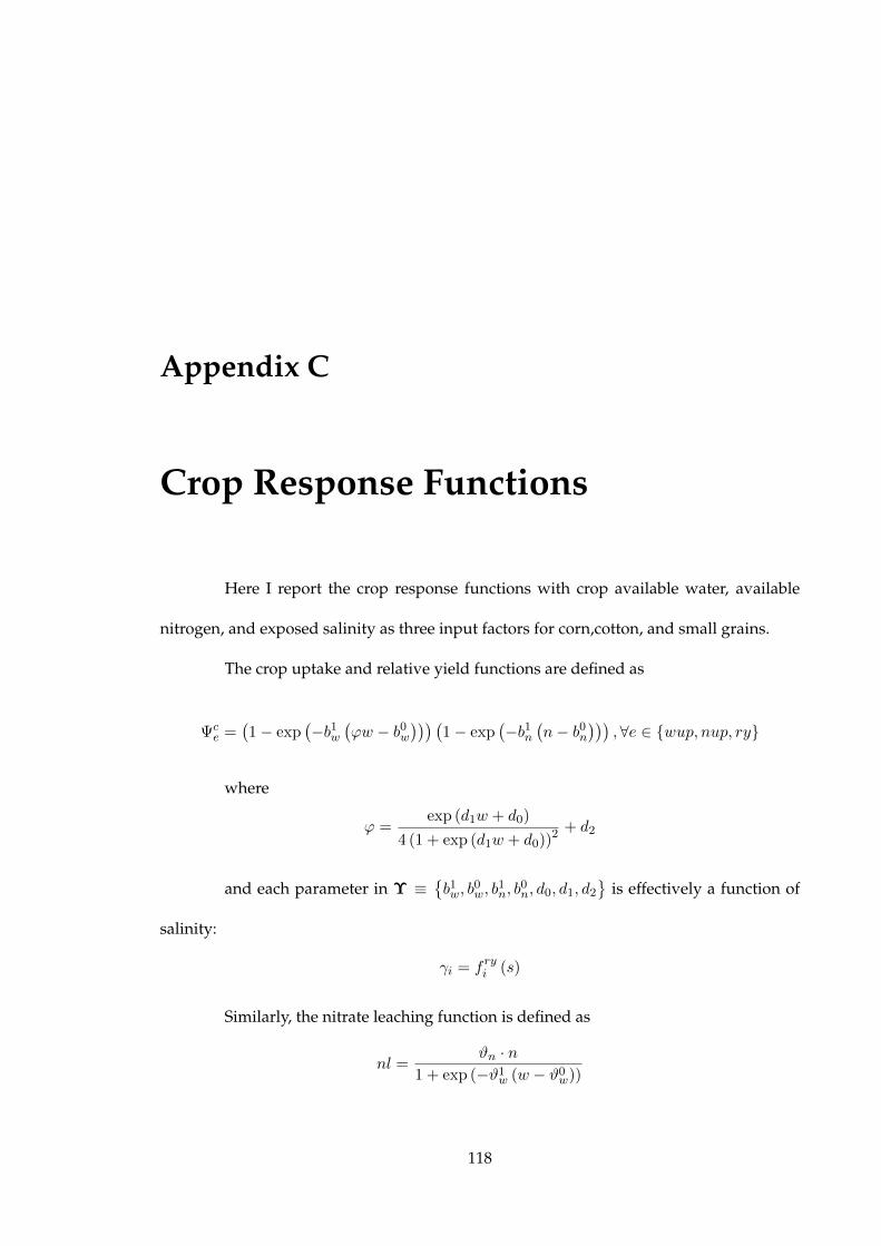
Appendix C

Crop Response Functions

Here I report the crop response functions with crop available water, available

nitrogen, and exposed salinity as three input factors for corn,cotton, and small grains.

The crop uptake and relative yield functions are defined as

Ψce =

(1− exp

(−b1w

(ϕw − b0w

))) (1− exp

(−b1n

(n− b0n

))), ∀e ∈ wup, nup, ry

where

ϕ =exp (d1w + d0)

4 (1 + exp (d1w + d0))2 + d2

and each parameter in Υ ≡b1w, b

0w, b

1n, b

0n, d0, d1, d2

is effectively a function of

salinity:

γi = f ryi (s)

Similarly, the nitrate leaching function is defined as

nl =ϑn · n

1 + exp (−ϑ1w (w − ϑ0w))

118

with parameters ϑ ≡ϑ1w, ϑ

0w, ϑn

depending on salinity levels:

ϑi = fnli (s)

119

Tabl

eC

.1:C

orn

resp

onse

func

tion

para

met

ers f i

(s)

Ψc

1s

s2s3

√s

R2

R2

b1 w0.

0185

2491

7-0

.000

7896

431.

9672

5E-0

5-1

.518

49E-

07–

0.99

77b0 w

-10.

0915

9346

-0.2

9085

8616

-0.0

2389

0955

0.00

0749

208

–0.

9816

b1 n–

––

––

–wup

b0 n–

––

––

–0.

9973

d0

-2.3

1659

422

0.07

0107

279

0.00

1985

563

-0.0

0015

3755

–0.

8090

d1

0.06

4861

651

-0.0

0030

1597

-1.4

6937

E-06

4.67

029E

-06

–0.

9855

d2

0.29

0408

999

0.00

6722

907

-0.0

0147

482.

5616

7E-0

5–

0.99

90b1 w

0.04

1659

821

-0.0

0062

4352

0.00

0196

842

-2.6

5171

E-06

–0.

9989

b0 w-3

8.41

5926

20.

3847

9338

40.

0604

4462

9-0

.001

4881

17–

0.99

92b1 n

0.00

7957

721

1.64

362E

-05

-2.6

4997

E-06

4.67

67E-

08–

0.99

61nup

b0 n-1

.184

9476

57-0

.007

2458

570.

0014

0375

5-3

.199

19E-

05–

0.88

000.

9956

d0

-1.0

6559

8703

-0.0

2859

8019

0.00

5495

742

-0.0

0011

5873

–0.

9941

d1

0.05

2346

560.

0007

3266

6-4

.790

9E-0

51.

3254

7E-0

6–

0.97

78d2

0.00

2855

162

0.00

0605

857

-0.0

0011

4209

2.91

392E

-06

–0.

7705

b1 w0.

0181

4311

5-0

.000

7078

741.

4785

3E-0

5-6

.511

48E-

08–

0.99

73b0 w

-10.

3161

4538

-0.2

4081

4603

-0.0

2696

0413

0.00

0804

812

–0.

9815

b1 n0.

0939

5855

10.

2153

0241

3-0

.015

3753

010.

0002

9392

3–

0.79

95ry

b0 n–

––

––

–0.

9973

d0

-2.1

7083

3492

0.03

9813

245

0.00

3750

585

-0.0

0018

4335

–0.

7736

d1

0.06

2725

976

0.00

0134

018

-2.6

2252

E-05

5.08

705E

-06

–0.

9846

d2

0.29

8695

498

0.00

4973

273

-0.0

0137

163

2.38

1E-0

5–

0.99

93ϑ1 w

0.41

4651

136

-0.0

2322

5526

0.00

0408

418

––

0.90

67nl

ϑ0 w

88.1

3923

159

0.00

4554

939

-0.0

0874

0355

––

0.97

340.

9734

ϑn

0.08

8789

230.

0066

4059

6-6

.824

1E-0

5–

–0.

9878

120

Tabl

eC

.2:C

otto

nre

spon

sefu

ncti

onpa

ram

eter

s* f i(s

)Ψc

1s

s2s3

√s

R2

R2

b1 w0.

0256

2592

7-0

.015

0731

01–

–0.

1095

9415

20.

9983

b0 w2.

8818

8044

8-0

.020

4881

04–

–-0

.369

3978

720.

9672

b1 n–

––

––

–wup

b0 n–

––

––

–0.

8835

d0

-0.1

9934

8185

-0.2

4459

4085

––

1.75

6989

507

0.99

97d1

0.03

0685

925

0.00

3583

966

––

-0.0

1575

2839

0.99

32d2

0.46

9486

895

0.00

4971

243

––

-0.0

9913

0962

0.97

49b1 w

0.04

1346

997

-0.0

0095

7879

0.00

0132

482

-2.0

0944

E-06

–0.

7922

b0 w-8

1.34

1687

7535

.930

9968

2-1

.129

0461

860.

0084

3462

6–

0.42

18b1 n

0.01

0013

821

8.44

799E

-05

-1.5

1659

E-05

2.55

119E

-07

–0.

9233

nup

b0 n-0

.057

7756

31-0

.040

0569

42-0

.045

2607

260.

0009

4217

6–

0.88

310.

9301

d0

-2.7

7227

6174

0.70

8780

628

-0.0

2569

0687

0.00

0236

486

–0.

3786

d1

0.02

3926

697

0.01

4263

124

-0.0

0067

2008

7.71

651E

-06

–0.

3584

d2

3.10

3187

249

-2.2

2474

0853

0.14

8163

111

-0.0

0197

7531

–0.

5799

b1 w0.

0345

8366

10.

0492

1352

5-0

.001

2738

916.

702E

-06

––

b0 w4.

5197

2892

-1.3

9798

3664

0.09

8234

258

––

–b1 n

0.03

3318

769

-0.0

0241

8865

0.00

0307

345

-4.2

2482

E-06

––

ryb0 n

0.04

1048

5-0

.003

1894

515.

9583

1E-0

5-3

.014

48E-

07–

–0.

7020

d0

0.24

1472

747

0.45

5173

526

-0.0

1683

0118

0.00

0158

142

––

d1

0.02

8166

739

-0.0

0125

1688

6.96

784E

-05

-4.2

9574

E-07

––

d2

0.40

4866

015

-0.1

0179

6477

0.00

6407

73–

––

ϑ1 w

0.12

1025

853

-0.0

0168

587

8.75

232E

-06

––

0.92

85nl

ϑ0 w

107.

6679

418

-0.1

3533

1412

-0.0

0555

1617

––

0.99

660.

9932

ϑn

0.24

9113

470.

0037

2874

3-1

.119

93E-

05–

–0.

9510

*ϕ

=ex

p(d

1w+d0)

4(1+ex

p(d

1w+d0))

2+

(d2)2

forwup

andnup

121

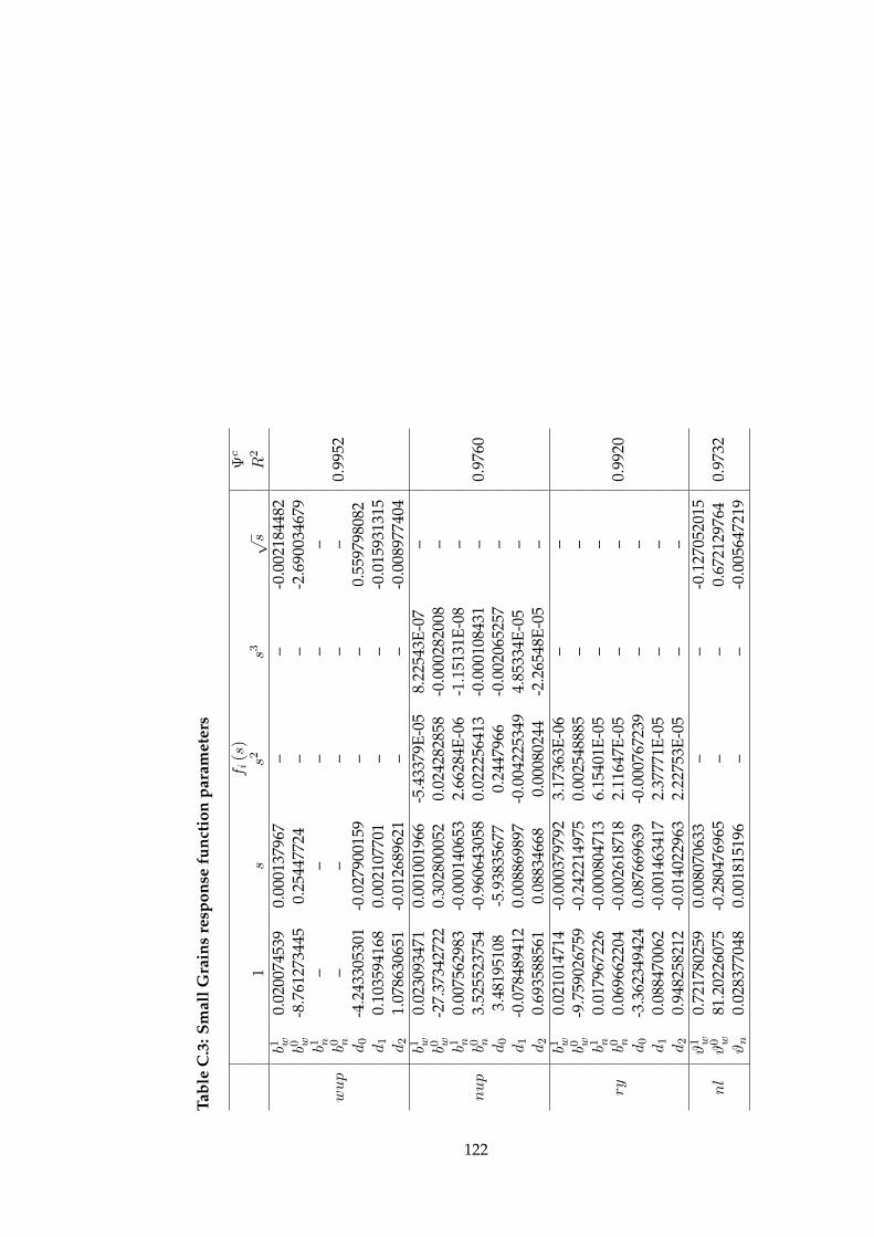
Tabl

eC

.3:S

mal

lGra

ins

resp

onse

func

tion

para

met

ers

f i(s

)Ψc

1s

s2s3

√s

R2

b1 w0.

0200

7453

90.

0001

3796

7–

–-0

.002

1844

82b0 w

-8.7

6127

3445

0.25

4477

24–

–-2

.690

0346

79b1 n

––

––

–wup

b0 n–

––

––

0.99

52d0

-4.2

4330

5301

-0.0

2790

0159

––

0.55

9798

082

d1

0.10

3594

168

0.00

2107

701

––

-0.0

1593

1315

d2

1.07

8630

651

-0.0

1268

9621

––

-0.0

0897

7404

b1 w0.

0230

9347

10.

0010

0196

6-5

.433

79E-

058.

2254

3E-0

7–

b0 w-2

7.37

3427

220.

3028

0005

20.

0242

8285

8-0

.000

2820

08–

b1 n0.

0075

6298

3-0

.000

1406

532.

6628

4E-0

6-1

.151

31E-

08–

nup

b0 n3.

5255

2375

4-0

.960

6430

580.

0222

5641

3-0

.000

1084

31–

0.97

60d0

3.48

1951

08-5

.938

3567

70.

2447

966

-0.0

0206

5257

–d1

-0.0

7848

9412

0.00

8869

897

-0.0

0422

5349

4.85

334E

-05

–d2

0.69

3588

561

0.08

8346

680.

0008

0244

-2.2

6548

E-05

–b1 w

0.02

1014

714

-0.0

0037

9792

3.17

363E

-06

––

b0 w-9

.759

0267

59-0

.242

2149

750.

0025

4888

5–

–b1 n

0.01

7967

226

-0.0

0080

4713

6.15

401E

-05

––

ryb0 n

0.06

9662

204

-0.0

0261

8718

2.11

647E

-05

––

0.99

20d0

-3.3

6234

9424

0.08

7669

639

-0.0

0076

7239

––

d1

0.08

8470

062

-0.0

0146

3417

2.37

771E

-05

––

d2

0.94

8258

212

-0.0

1402

2963

2.22

753E

-05

––

ϑ1 w

0.72

1780

259

0.00

8070

633

––

-0.1

2705

2015

nl

ϑ0 w

81.2

0226

075

-0.2

8047

6965

––

0.67

2129

764

0.97

32ϑn

0.02

8377

048

0.00

1815

196

––

-0.0

0564

7219

122

Appendix D

Farm Model Parameters

123

Tabl

eD

.1:A

nim

alM

odel

Para

met

ers

Sym

bol

Des

crip

tion

Val

ueSo

urce

fal

falf

a,w

heat

sila

ge,c

orn

grai

n,so

ybea

nm

eal,

and

prot

ein

mix

cons

umed

byca

lves

,hei

fers

,an

dco

ws

[kg/

anim

al/y

r]

270

690

861

861

2143

2621

522

102

3296

00

130

015

1

R

otz

etal

.[19

99]

Baer

enkl

auet

al.[

2008

]

fsw

1w

ater

cons

umpt

ion

unde

rflu

sh-l

agoo

nsy

stem

[m3 /a

nim

al/y

r][1.4

2,3.

37,2

41.7

7]Ba

eren

klau

etal

.[20

08]

Bray

etal

.[20

11]

fsw

2w

ater

cons

umpt

ion

unde

rsc

rape

-tan

ksy

stem

[m3 /a

nim

al/y

r][1.4

2,3.

37,1

31.2

4]Ba

eren

klau

etal

.[20

08]

Bray

etal

.[20

11]

pfe

ed

feed

pric

e[$

/kg]

[0.1

624,

0.14

32,0.1

444,

0.30

08,0.3

971]

Baer

enkl

auet

al.[

2008

]m

ilkpr

oduc

edby

coho

rt[$

/ani

mal

/yr]

[0,0,9

642]

Rot

zet

al.[

1999

]pM 1

annu

aliz

edco

stof

flush

-lag

oon

syst

em[$

/cow

/yr]

50Be

nnet

teta

l.[1

994]

pM 2

annu

aliz

edco

stof

scra

pe-t

ank

syst

em[$

/cow

/yr]

150

Benn

ette

tal.

[199

4]

pmilk

pric

eof

milk

[$/k

g]0.3

1C

DFA

[201

0]psw

pric

eof

impo

rted

surf

ace

wat

er[$

/m3 ]

0.02

58V

arga

set

al.[

2003

]p

herd

pric

esof

selli

ngco

hort

s[$

/ani

mal

][3

53,8

38,6

33]

Baer

enkl

auet

al.[

2008

]p

fixh

herd

prod

ucti

onfix

edco

st[$

/ani

mal

/yr]

[0,0,1

309]

Rot

zet

al.[

2003

]psol

pric

ere

ceiv

edfo

rdr

ied

solid

was

te[$

/kgN

]0.1

4Ba

eren

klau

etal

.[20

08]

pbase

the

base

pric

efo

rha

ulin

gm

anur

eof

f-si

te[$

/ha-

cm]

201.8

3Fl

emin

get

al.[

1998

]

pdist

the

haul

ing

cost

per

unit

dist

ance

[$/h

a-cm

-km

]54.0

2Fl

emin

get

al.[

1998

]

124

Tabl

eD

.2:C

rop

and

Hyd

rolo

gic

Mod

elPa

ram

eter

s

Sym

bol

Des

crip

tion

Val

ueSo

urce

prec k

prec

ipit

atio

ndu

ring

the

sum

mer

and

win

ter

grow

ing

seas

on[c

m]

[2,1

]C

IMIS

δ km

iner

aliz

atio

nra

teof

orga

nic

nitr

ogen

duri

ngth

esu

mm

eran

dw

inte

rgr

owin

gse

ason

[0.4

73,0.2

04]

Cha

nget

al.[

2005

]

φth

efr

acti

onof

appl

ied

liqui

dw

aste

nitr

ogen

that

vola

tiliz

esdu

ring

appl

icat

ion

0.2

5C

hang

etal

.[20

05]

λde

nitr

ifica

tion

rate

inth

eun

satu

rate

dzo

ne0.2

5M

eisi

nger

and

Ran

dall

[198

8]ν

field

capa

city

ofth

eso

il[c

m]

30U

SDA

[200

7b]

nca

nitr

ogen

conc

entr

atio

nof

surf

ace

wat

er,d

eep

grou

ndw

ater

,and

prec

ipit

atio

n[k

gN/h

a-cm

][0.1,1,0.1

]Sc

hans

[200

1]

eca

elec

tric

alco

nduc

tivi

tyof

surf

ace

wat

er,d

eep

grou

ndw

ater

,and

prec

ipit

atio

n[d

S/m

][0.1

5,1.1

83,0.1

]Sc

hans

[200

1]

pgw

cost

ofus

ing

deep

grou

ndw

ater

[$/h

a-cm

]8.8

4R

uud

etal

.[20

03]

prw

cost

ofus

ing

shal

low

grou

ndw

ater

[$/h

a-cm

]2.5

8R

uud

etal

.[20

03]

pfl

cost

ofch

emic

alfe

rtili

zers

[$/k

gN]

0.5

9K

napp

and

Schw

abe

[200

8]αdenitri

nitr

ate

loss

rate

due

tode

nitr

ifica

tion

inth

esa

tura

ted

zone

0.0

2D

eSim

one

and

How

es[1

998]

αmiscel

nitr

ate

loss

rate

due

toth

eot

her

tran

sfor

mat

ion

proc

esse

sin

the

satu

rate

dzo

ne0.1

6D

eSim

one

and

How

es[1

998]

125

Appendix E

Mathematica Code

(*Dynamic Model of Animal-Crop Operations_Model*)(*Jingjing Wang, 2012*)(*Flush - lagoon system : nonuniform application of both water and manure*)(*Codes for data input, crop response functions,and start points generation are available upon request*)

ClearAll[h3, soilorg, soilinorg, soilec,plantnitrogen,plantec,wateruptake,nitrogenuptake,nitrogenleaching,nmassiw, ecmassiw]

(*State variable*)h3All:=Array[h3, T,G]soilorgAll:=Array[soilorg, T,K, J]soilinorgAll:=Array[soilinorg, T,K, J]soilecAll:=Array[soilec, T,K, J]

(*Intermediate variable*)plantnitrogenAll:=Array[plantnitrogen, T,K, J]plantecAll:=Array[plantec, T,K, J]wateruptakeAll:=Array[wateruptake, T,K, J]nitrogenuptakeAll:=Array[nitrogenuptake, T,K, J]nitrogenleachingAll:=Array[nitrogenleaching, T,K, J]

(***HerdManagement***)

ClearAll[θ, h, θθ,hCull, animal, πh]θ3All:=Array[θ, T,G]h[t_,g_]:=calve,heifer, 1 ∗ h3[t, g]

126

θθ[t_,g_]:=calve,heifer, 1 ∗ θ[t, g]hCull[t_,g_]:=(bullcalf + calfcull) ∗ h3[t, g],heifercull ∗ h3[t, g], cowcull ∗ h3[t, g]animal[t_,g_]:=animalunit.calve,heifer, 1 ∗ h3[t, g]

(*Economic Submodel for Herd Production*)πh[t_]:=Sum[pmilk ∗ ymilk ∗ h3[t, g] + pherd.hCull[t, g]− pherd.θθ[t, g]−consump.pconsump.h[t, g]− pwaterherd ∗ consumpWater.h[t, g]−pfixherd.h[t, g]− pcollect ∗ h3[t, g], g,G]hvars:=Flatten[h3All, θ3All]hcons:=Join[hcons1,hcons2,hcons3]hcons1:=Table[herdpermit ≥ animal[t, g] ≥ 0, t, T, g,G]hcons2:=Table[0==h3[t, g − 1] + θ[t, g]− h3[t, g], g, 2, G, t, 1, T]hcons3:=Table[0==h3[t− 1, G] + θ[t, 1]− h3[t, 1], t, 1, T]

(***ManureManagement***)

ClearAll[lonsite, sonsite, lonsitefield, sonsitefield, lvonsite, lvoffsite, solidN,liquidorgN, liquidinorgN, liquidN, landtosearch, rbig, raverage,phauling, πwaste]lonsiteAll:=Array[lonsite, T,K];sonsiteAll:=Array[sonsite, T,K];lonsitefield[t_,k_]:=(landonsite− pond)lonsite[t, k];sonsitefield[t_,k_]:=(landonsite− pond)sonsite[t, k];lvonsite[t_,k_]:=lonsite[t, k] ∗wPERnlvoffsite[t_,g_]:=(liquidN[t, g]− Sum[lonsitefield[t, k], k, 2g − 1, 2g]) ∗wPERn

(*manure production*)solidN[t_,g_]:=flow1flow8((1− flow2)urineN + fecalN(1− flow3)).h[t, g];liquidorgN[t_,g_]:=(1− flow1 ∗ flow8)(urineN(1− flow2) + fecalN(1− flow3)).h[t, g];liquidinorgN[t_,g_]:=((urineNflow2 + fecalNflow3)flow1(1− flow5)(1− flow6)+(urineNflow2 + fecalNflow3)(1− flow1)(1− flow4)).h[t, g];liquidN[t_,g_]:=((1− flow1 ∗ flow8)(urineN(1− flow2) + fecalN(1− flow3))+(urineNflow2 + fecalNflow3)flow1(1− flow5)(1− flow6)+(urineNflow2 + fecalNflow3)(1− flow1)(1− flow4)).h[t, g];

(*offsite manure disposal*)landtosearch[t_,g_]:=(liquidN[t, g]− Sum[lonsitefield[t, k], k, 2g − 1, 2g])/offsiteRate/offsiteFraction/wtam

rbig[t_,g_]:=√

landtosearch[t,g]+landonsite100π ;

rsmall =√

landonsite100π ;

raverage[t_,g_]:=2(rbig[t,g]2+rbig[t,g]∗rsmall+rsmall2)

3(rbig[t,g]+rsmall)phauling[t_,g_]:=(pbase + pdist ∗ raverage[t, g]) ∗ lvoffsite[t, g]

(*Economic Submodel for Waste Disposal*)

127

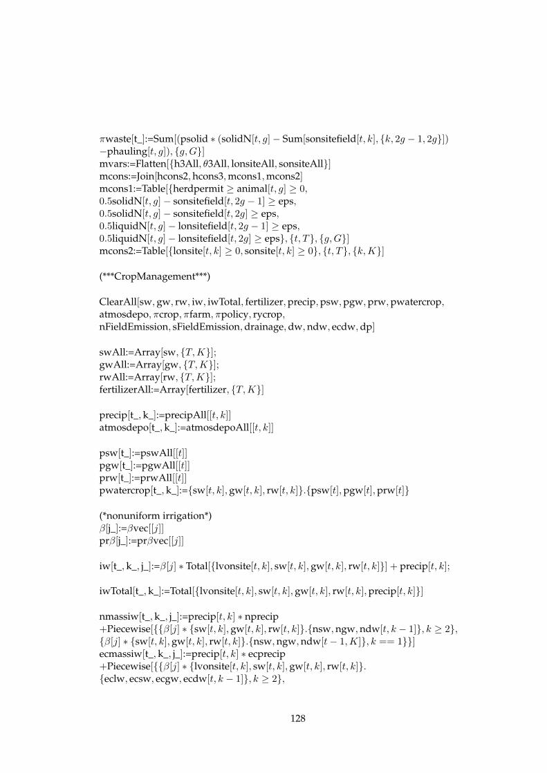
πwaste[t_]:=Sum[(psolid ∗ (solidN[t, g]− Sum[sonsitefield[t, k], k, 2g − 1, 2g])−phauling[t, g]), g,G]mvars:=Flatten[h3All, θ3All, lonsiteAll, sonsiteAll]mcons:=Join[hcons2,hcons3,mcons1,mcons2]mcons1:=Table[herdpermit ≥ animal[t, g] ≥ 0,0.5solidN[t, g]− sonsitefield[t, 2g − 1] ≥ eps,0.5solidN[t, g]− sonsitefield[t, 2g] ≥ eps,0.5liquidN[t, g]− lonsitefield[t, 2g − 1] ≥ eps,0.5liquidN[t, g]− lonsitefield[t, 2g] ≥ eps, t, T, g,G]mcons2:=Table[lonsite[t, k] ≥ 0, sonsite[t, k] ≥ 0, t, T, k,K]

(***CropManagement***)

ClearAll[sw,gw, rw, iw, iwTotal, fertilizer,precip,psw,pgw,prw,pwatercrop,atmosdepo, πcrop, πfarm, πpolicy, rycrop,nFieldEmission, sFieldEmission,drainage,dw,ndw, ecdw,dp]

swAll:=Array[sw, T,K];gwAll:=Array[gw, T,K];rwAll:=Array[rw, T,K];fertilizerAll:=Array[fertilizer, T,K]

precip[t_,k_]:=precipAll[[t, k]]atmosdepo[t_,k_]:=atmosdepoAll[[t, k]]

psw[t_]:=pswAll[[t]]pgw[t_]:=pgwAll[[t]]prw[t_]:=prwAll[[t]]pwatercrop[t_,k_]:=sw[t, k],gw[t, k], rw[t, k].psw[t],pgw[t],prw[t]

(*nonuniform irrigation*)β[j_]:=βvec[[j]]prβ[j_]:=prβvec[[j]]

iw[t_,k_, j_]:=β[j] ∗ Total[lvonsite[t, k], sw[t, k],gw[t, k], rw[t, k]] + precip[t, k];

iwTotal[t_,k_]:=Total[lvonsite[t, k], sw[t, k],gw[t, k], rw[t, k],precip[t, k]]

nmassiw[t_,k_, j_]:=precip[t, k] ∗ nprecip+Piecewise[β[j] ∗ sw[t, k],gw[t, k], rw[t, k].nsw,ngw,ndw[t, k − 1], k ≥ 2,β[j] ∗ sw[t, k],gw[t, k], rw[t, k].nsw,ngw,ndw[t− 1,K], k == 1]ecmassiw[t_,k_, j_]:=precip[t, k] ∗ ecprecip+Piecewise[β[j] ∗ lvonsite[t, k], sw[t, k],gw[t, k], rw[t, k].eclw, ecsw, ecgw, ecdw[t, k − 1], k ≥ 2,

128

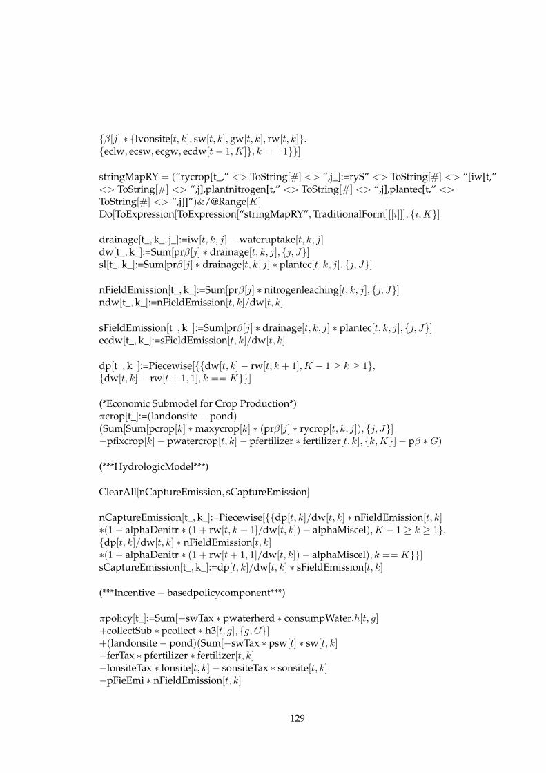
β[j] ∗ lvonsite[t, k], sw[t, k],gw[t, k], rw[t, k].eclw, ecsw, ecgw, ecdw[t− 1,K], k == 1]

stringMapRY = (“rycrop[t_,” <> ToString[#] <> “,j_]:=ryS” <> ToString[#] <> “[iw[t,”<> ToString[#] <> “,j],plantnitrogen[t,” <> ToString[#] <> “,j],plantec[t,” <>ToString[#] <> “,j]]”)&/@Range[K]Do[ToExpression[ToExpression[“stringMapRY”,TraditionalForm][[i]]], i,K]

drainage[t_,k_, j_]:=iw[t, k, j]−wateruptake[t, k, j]dw[t_,k_]:=Sum[prβ[j] ∗ drainage[t, k, j], j, J]sl[t_,k_]:=Sum[prβ[j] ∗ drainage[t, k, j] ∗ plantec[t, k, j], j, J]

nFieldEmission[t_,k_]:=Sum[prβ[j] ∗ nitrogenleaching[t, k, j], j, J]ndw[t_,k_]:=nFieldEmission[t, k]/dw[t, k]

sFieldEmission[t_,k_]:=Sum[prβ[j] ∗ drainage[t, k, j] ∗ plantec[t, k, j], j, J]ecdw[t_,k_]:=sFieldEmission[t, k]/dw[t, k]

dp[t_,k_]:=Piecewise[dw[t, k]− rw[t, k + 1],K − 1 ≥ k ≥ 1,dw[t, k]− rw[t+ 1, 1], k == K]

(*Economic Submodel for Crop Production*)πcrop[t_]:=(landonsite− pond)(Sum[Sum[pcrop[k] ∗maxycrop[k] ∗ (prβ[j] ∗ rycrop[t, k, j]), j, J]−pfixcrop[k]− pwatercrop[t, k]− pfertilizer ∗ fertilizer[t, k], k,K]− pβ ∗G)

(***HydrologicModel***)

ClearAll[nCaptureEmission, sCaptureEmission]

nCaptureEmission[t_,k_]:=Piecewise[dp[t, k]/dw[t, k] ∗ nFieldEmission[t, k]∗(1− alphaDenitr ∗ (1 + rw[t, k + 1]/dw[t, k])− alphaMiscel),K − 1 ≥ k ≥ 1,dp[t, k]/dw[t, k] ∗ nFieldEmission[t, k]∗(1− alphaDenitr ∗ (1 + rw[t+ 1, 1]/dw[t, k])− alphaMiscel), k == K]sCaptureEmission[t_,k_]:=dp[t, k]/dw[t, k] ∗ sFieldEmission[t, k]

(***Incentive− basedpolicycomponent***)

πpolicy[t_]:=Sum[−swTax ∗ pwaterherd ∗ consumpWater.h[t, g]+collectSub ∗ pcollect ∗ h3[t, g], g,G]+(landonsite− pond)(Sum[−swTax ∗ psw[t] ∗ sw[t, k]−ferTax ∗ pfertilizer ∗ fertilizer[t, k]−lonsiteTax ∗ lonsite[t, k]− sonsiteTax ∗ sonsite[t, k]−pFieEmi ∗ nFieldEmission[t, k]

129

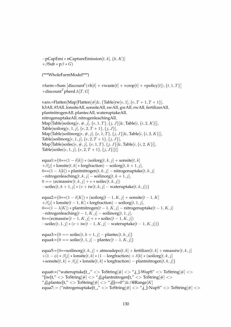
−pCapEmi ∗ nCaptureEmission[t, k], k,K]+βSub ∗ pβ ∗G)

(***WholeFarmModel***)

πfarm:=Sum[discountt(πh[t] + πwaste[t] + πcrop[t] + πpolicy[t]), t, 1, T

]+discountTpherd.h[T,G]

vars:=Flatten[Map[Flatten[#]&, Table[rw[e, 1], e, T + 1, T + 1],h3All, θ3All, lonsiteAll, sonsiteAll, swAll,gwAll, rwAll, fertilizerAll,plantnitrogenAll,plantecAll,wateruptakeAll,nitrogenuptakeAll,nitrogenleachingAll,Map[Table[soilorg[e,#, j], e, 1, T, j, J]&,Table[i, i, 2,K]],Table[soilorg[e, 1, j], e, 2, T + 1, j, J],Map[Table[soilinorg[e,#, j], e, 1, T, j, J]&,Table[i, i, 2,K]],Table[soilinorg[e, 1, j], e, 2, T + 1, j, J],Map[Table[soilec[e,#, j], e, 1, T, j, J]&,Table[i, i, 2,K]],Table[soilec[e, 1, j], e, 2, T + 1, j, J]]]

equa1:=0==(1− δ[k]) ∗ (soilorg[t, k, j] + sonsite[t, k]+β[j] ∗ lonsite[t, k] ∗ lorgfraction)− soilorg[t, k + 1, j],0==(1− λ[k]) ∗ plantnitrogen[t, k, j]− nitrogenuptake[t, k, j]−nitrogenleaching[t, k, j]− soilinorg[t, k + 1, j],0 == (ecmassiw[t, k, j] + v ∗ soilec[t, k, j])−soilec[t, k + 1, j] ∗ (v + iw[t, k, j]−wateruptake[t, k, j])

equa2:=0==(1− δ[K]) ∗ (soilorg[t− 1,K, j] + sonsite[t− 1,K]+β[j] ∗ lonsite[t− 1,K] ∗ lorgfraction)− soilorg[t, 1, j],0==(1− λ[K]) ∗ plantnitrogen[t− 1,K, j]− nitrogenuptake[t− 1,K, j]−nitrogenleaching[t− 1,K, j]− soilinorg[t, 1, j],0==(ecmassiw[t− 1,K, j] + v ∗ soilec[t− 1,K, j])−soilec[t, 1, j] ∗ (v + iw[t− 1,K, j]−wateruptake[t− 1,K, j])

equa3:=0 == soilec[t, k + 1, j]− plantec[t, k, j]equa4:=0 == soilec[t, 1, j]− plantec[t− 1,K, j]

equa5:=0==soilinorg[t, k, j] + atmosdepo[t, k] + fertilizer[t, k] + nmassiw[t, k, j]+(1− φ) ∗ β[j] ∗ lonsite[t, k] ∗ (1− lorgfraction) + δ[k] ∗ (soilorg[t, k, j]+sonsite[t, k] + β[j] ∗ lonsite[t, k] ∗ lorgfraction)− plantnitrogen[t, k, j]

equa6:=(“wateruptake[t_,” <> ToString[#] <> “,j_]-WupS” <> ToString[#] <>“[iw[t,” <> ToString[#] <> “,j],plantnitrogen[t,” <> ToString[#] <>“,j],plantec[t,” <> ToString[#] <> “,j]]==0”)&/@Range[K]equa7; = (“nitrogenuptake[t_,” <> ToString[#] <> “,j_]-NupS” <> ToString[#] <>

130

“[iw[t,” <> ToString[#] <> “,j],plantnitrogen[t,” <> ToString[#] <>“,j],plantec[t,” <> ToString[#] <> “,j]]==0”)&/@Range[K]equa8; = (“nitrogenleaching[t_,” <> ToString[#] <> “,j_]-nlS” <> ToString[#] <>“[iw[t,” <> ToString[#] <> “,j],plantnitrogen[t,” <> ToString[#] <>“,j],plantec[t,” <> ToString[#] <> “,j]]==0”)&/@Range[K]

cons11:=Table[equa1, t, T, k,K − 1, j, J]cons22:=Table[equa2, t, 2, T + 1, j, J]cons33:=Table[equa3, t, T, k,K − 1, j, J]cons44:=Table[equa4, t, 2, T + 1, j, J]cons55:=Table[equa5, t, T, k,K, j, J]cons66:=Table[equa6, t, T, j, J]cons77:=Table[equa7, t, T, j, J]cons88:=Table[equa8, t, T, j, J]

inequa1:=herdpermit ≥ animal[t, g] ≥ eps,0.5solidN[t, g]− sonsitefield[t, 2g − 1] ≥ eps,0.5solidN[t, g]− sonsitefield[t, 2g] ≥ eps,0.5liquidN[t, g]− lonsitefield[t, 2g − 1] ≥ eps,0.5liquidN[t, g]− lonsitefield[t, 2g] ≥ epsinequa2:=200 ≥ soilec[t, k, j] ≥ epsinequa3:=6000 ≥ lonsite[t, k] ≥ eps, 6000 ≥ sonsite[t, k] ≥ eps,wLimit[k] ≥ iwTotal[t, k], sw[t, k] ≥ eps,gw[t, k] ≥ eps, rw[t, k] ≥ eps,400 ≥ fertilizer[t, k] ≥ eps,dp[t, k] ≥ eps

cons1:=Table[inequa1, t, T, g,G]cons2:=Table[inequa2, t, T, k, 2,K, j, J]cons3:=Table[inequa3, t, T, k,K]cons4:=rw[T + 1, 1] ≥ epscons:=Flatten[Table[Nest[Flatten[#]&, i, 2], i, cons11, cons22, cons33, cons44,cons55, cons66, cons77, cons88, cons1, cons2, cons3, cons4,hcons2,hcons3]]

(*NMPs*)inequaPolicy:=1.4 ∗NupMax[k] ≥ lonsite[t, k] ∗ (1− lorgfraction)+δ[k] ∗ (sonsite[t, k] + lonsite[t, k] ∗ lorgfraction)+fertilizer[t, k] + Sum[prβ[j] ∗ nmassiw[t, k, j], j, J]consPolicy:=Table[inequaPolicy, t, T, k,K]

(*whole farm optimization*)

πfarmMax = KnitroMaximize[πfarm, Join[cons,Flatten[consPolicy]], , startpoint,ReturnAsRules→ True,TraceProgress→ True,Hessian→ “SR1”,MaxIterations→ 8000,KnitroOptionList→ “xtol”, 0.1∧8, “Algorithm”, 2,“outmode”, 1, “outlev”, 5, “log_knml”, 1]//AbsoluteTiming

131