An Investigation of Missing Data Methods for Classification Trees ...

Journal of Machine Learning Research 11 (2010) 131-170 Submitted 4/09; Revised 12/09; Published 1/10

An Investigation of Missing Data Methods for Classification TreesApplied to Binary Response Data

Yufeng Ding [email protected]

Moody’s Investors Service250 Greenwich StreetNew York, NY 10007

Jeffrey S. Simonoff [email protected] .EDU

New York University, Stern School of Business44 West 4th StreetNew York, NY 10012

Editor: Charles Elkan

Abstract

There are many different methods used by classification treealgorithms when missing data occur inthe predictors, but few studies have been done comparing their appropriateness and performance.This paper provides both analytic and Monte Carlo evidence regarding the effectiveness of sixpopular missing data methods for classification trees applied to binary response data. We show thatin the context of classification trees, the relationship between the missingness and the dependentvariable, as well as the existence or non-existence of missing values in the testing data, are the mosthelpful criteria to distinguish different missing data methods. In particular, separate class is clearlythe best method to use when the testing set has missing valuesand the missingness is related tothe response variable. A real data set related to modeling bankruptcy of a firm is then analyzed.The paper concludes with discussion of adaptation of these results to logistic regression, and otherpotential generalizations.

Keywords: classification tree, missing data, separate class, RPART, C4.5, CART

1. Classification Trees and the Problem of Missing Data

Classification trees are a supervised learning method appropriate for datawhere the response vari-able is categorical. The simple methodology behind classification trees is to recursively split databased upon the predictors that best distinguish the response variable classes. There are, of course,many subtleties, such as the choice of criterion function used to pick the bestsplit variable, stoppingrules, pruning rules, and so on. In this study, we mostly rely on the built-in features of the tree algo-rithms C4.5 andRPART to implement tree methods. Details about classification trees can be foundin various references, for example, Breiman, Friedman, Olshen, and Stone (1998) and Quinlan(1993). Classification trees are computationally efficient, can handle mixed variables (continuousand discrete) easily and the rules generated by them are relatively easy tointerpret and understand.Classification trees are highly flexible, and naturally uncover interaction effects among the inde-pendent variables. Classification trees are also popular because they can easily be incorporated intolearning ensembles or larger learning systems as base learners.

c©2010 Yufeng Ding and Jeffrey S. Simonoff.

DING AND SIMONOFF

Like most statistics or machine learning methods, “base form” classification trees are designedassuming that data are complete. That is, all of the values in the data matrix, with the rows being theobservations (instances) and the columns being the variables (attributes),are observed. However,missing data (meaning that some of the values in the data matrix are not observed) is a very commonproblem, and for this reason classification trees have to, and do, have ways of dealing with missingdata in the predictors. (In supervised learning, an observation with missingresponse value has noinformation about the underlying relationship, and must be omitted. There is, however, research inthe field of semi-supervised learning methods that tries to handle the situation where the responsevalue is missing, for example, Wang and Shen 2007.)

Although there are many different ways of dealing with missing data in classification trees,there are relatively few studies in the literature about the appropriatenessand performance of thesemissing data methods. Moreover, most of these studies limited their coverage to the simplest miss-ing data scenario, namely, missing completely at random (MCAR), while our study shows that themissing data generating process is one of the two crucial criteria in determiningthe best missingdata method. The other crucial criterion is whether or not the testing set is complete. The followingtwo subsections describe in more detail these two criteria.

1.1 Different Types of Missing Data Generating Process

Data originate according to the data generating process (DGP) under which the data matrix is “gen-erated” according to the probabilistic relationships between the variables. We can think of themissingness itself as a random variable, realized as the matrix of the missingness indicatorIm. Im isgenerated according to the missingness generating process (MGP), which governs the relationshipbetweenIm and the variables in the data matrix.Im has the same dimension as the original datamatrix, with each entry equal to 0 if the corresponding original data value is observed and 1 if thecorresponding original data value is not observed (missing). Note that an Im value not only can berelated to its corresponding original data value, but can also be related to other variables of the sameobservation.

Depending on the relationship betweenIm and the original data, Rubin (1976) and Little and Ru-bin (2002) categorize the missingness into three different types. IfIm is dependent upon the missingvalues (the unobserved original data values), then the missingness pattern is called “not missing atrandom” (NMAR). Otherwise, the missingness pattern is called “missing at random” (MAR). As aspecial case of MAR, when the missingness is also not dependent on the observed values (that is,is independent of all data values), the missingness pattern is called “missing completely at random”(MCAR). The definition of MCAR is rather restrictive, which makes MCAR unlikely in reality. Forexample, in the bankruptcy data discussed later in the paper, there is evidence that after the Enronscandal in 2001, when both government and the public became more wary about financial reportingmisconduct, missingness of values in financial statement data was related to thewell-being of thecompany, and thus other values in the data. This makes intuitive sense because when scrutinized, acompany is more likely to have trouble reporting their financial data if there were problems. Thus,focusing on the MCAR case is a major limitation that will be avoided in this paper. Infact, thispaper shows that the categorization of MCAR, MAR and NMAR itself is not appropriate for themissing data problem in classification trees, as well as in another supervisedlearning context (atleast with respect to prediction), although it has been shown to be helpfulwith likelihood-based orBayesian analysis.

132

AN INVESTIGATION OF M ISSING DATA METHODS FORCLASSIFICATION TREES

Missingness is related toMissing Observed Responsevalues Predictors Variable LR Three-Letter

1 No No No MCAR −−−

2 No Yes No MAR −X−

3 Yes No No NMAR M −−

4 Yes Yes No NMAR M X−

5 No No Yes MAR −−Y6 No Yes Yes MAR −X Y7 Yes No Yes NMAR M −Y8 Yes Yes Yes NMAR M X Y

Table 1: Eight missingness patterns investigated in this study and their correspondence to the cate-gorization MCAR, MAR and NMAR defined by Rubin (1976) and Little and Rubin (2002)(the LR column). The column Three-Letter shows the notation that is used in thispaper.

In this paper, we investigate eight different missingness patterns, depending on the relationshipbetween the missingness and three types of variables, the observed predictors, the unobserved pre-dictors (the missing values) and the response variable. The relationship is conditional upon otherfactors, for example, missingness is not dependent upon the missing values means that the miss-ingness is conditionally independent of the missing values given the observed predictors and/orthe response variable. Table 1 shows their correspondence with the MCAR/MAR/NMAR catego-rization as well as the three-letter notation we use in this paper. The three letters indicate if themissingness is conditionally dependent on the missing values (M), on other predictors (X) and onthe response variable (Y), respectively. As will be shown, the dependence of the missingness on theresponse variable (the letter Y) is the one that affects the choice of best missingness data method.Later in the paper, some derived notations are also used. For example,∗X∗ means the union of−X−, −XY, MX− and MXY, that is, the missingness is dependent upon the observed predictors,and it may or may not be related to the missing values and/or the response variable.

1.2 Scenarios Where the Testing Data May or May Not Be Complete

There are essentially two stages of applying classification trees, the trainingphase where the his-torical data (training set) are used to construct the tree, and the testing phase where the tree is putinto use and applied to testing data. Similar to most other studies, this study deals withthe scenariowhere missing data occur in the training set, but the testing set may or may not have missing values.One basic assumption is, of course, that the DGP (as well as MGP if the testingset also containsmissing values) is the same for both the training set and the testing set.

While it would probably typically be the case that the testing data would also havemissing val-ues (generated by the same process that generated them in the training set), it should be noted that incertain circumstances a testing set without missing values could be expected.For example, considera problem involving prediction of bankruptcy from various financial ratios. If the training set comesfrom a publicly available database, there could be missing values corresponding to information thatwas not supplied by various companies. If the goal is to use these publicly available data to try

133

DING AND SIMONOFF

to predict bankruptcy from ratios from one’s own company, it would be expected that all of thenecessary information for prediction would be available, and thus the test set would be complete.

This study shows that when the missingness is dependent upon the response variable and thetest set has missing values, separate class is the best missing data method to use. In other situations,the choice is not as clear, but some insights on effective choices are provided. The rest of paperprovides detailed theoretical and empirical analysis and is organized as follows. Section 2 gives abrief introduction to the previous research on this topic. This is followed by discussion of the designof this study and findings in Section 3. The generality of the results are then tested on real data setsin Section 4. A brief extension of the results to logistic regression is presented in Section 5. Weconclude with discussion of these results and future work in Section 6.

2. Previous Research

There have been several studies of missing data and classification trees inthe literature. Liu, White,Thompson, and Bramer (1997) gave a general description of the problem, but did not discuss solu-tions. Saar-Tsechansky and Provost (2007) discussed various missing data methods in classificationtrees and proposed a cost-sensitive approach to the missing data problemfor the scenario when miss-ing data occur only at the testing phase, which is different from the problem studied here (wheremissing values occur in the training phase).

Kim and Yates (2003) conducted a simulation study of seven popular missing value methodsbut did not find any dominant method. Feelders (1999) compared the performance of surrogate splitand imputation and found the imputation methods to work better. (These methods, and the methodsdescribed below, are described more fully in the next section.) Batista and Monard (2003) comparedfour different missing data methods, and found that 10 nearest neighbor imputation outperformedother methods in most cases. In the context of cost sensitive classificationtrees, Zhang, Qin, Ling,and Sheng (2005) studied four different missing data methods based on their performances on fivedata sets with artificially generated random missing values. They concluded that the internal nodemethod (the decision rules for the observations with the next split variable missing will be madeat the (internal) node) is better than the other three methods examined. Fujikawa and Ho (2002)compared several imputation methods based on preliminary clustering algorithmsto probabilisticsplit on simulations based on several real data sets and found comparableperformance. A weaknessof all of the above studies is that they focused only on the restrictive MCARsituation.

Other studies examined both MAR and NMAR missingness. Kalousis and Hilario (2000) usedsimulations from real data sets to examine the properties of seven algorithms: two rule inducers, anearest neighbor method, two decision tree inducers, a naive Bayes inducer, and linear discriminantanalysis. They found that the naive Bayes method was by far most resilient to missing data, inthe sense that its properties changed the least when the missing rate was increased (note that thisresilience is related to, but not the same as, its overall predictive performance). They also foundthat the deleterious effects of missing data are more serious if a given amount of missing values arespread over several variables, rather than concentrated in a few.

Twala (2009) used computer simulations based on real data sets to compare the properties ofdifferent missing value methods, including using complete cases, single imputation of missing val-ues, likelihood-based multiple imputation (where missing values are imputed several times, andthe results of fitting trees to the different generated data sets are combined),probabilistic split, andsurrogate split. He studied MAR, MCAR, and NMAR missingness generating processes, although

134


dependence of missingness on the response variable was not examined.Multiple imputation wasfound to be most effective, with probabilistic split also performing reasonably well, although littledifference was found between methods when the proportion of missing values was low. As wouldbe expected, MCAR missingness caused the least problems for methods, while NMAR missingnesscaused the most, and as was also found by Kalousis and Hilario (2000), missingness spread overseveral predictors is more serious than if it is concentrated in only one. Twala, Jones, and Hand(2008) proposed a method closely related to creating a separate class formissing values, and foundthat its performance was competitive with that of likelihood-based multiple imputation.

The study described in the next section extends these previous studies in several ways. First,theoretical analyses are provided for simple situations that help explain observed empirical perfor-mance. We then extend these analyses to more complex situations and data sets (including largeones) using Monte Carlo simulations based on generated and real data sets. The importance ofwhether missing is dependent on the response variable, which has been ignored in previous studieson classification trees yet turns out to be of crucial importance, is a fundamental aspect of theseresults. The generality of the conclusions is finally tested using real data sets and application tologistic regression.

3. The Effectiveness of Missing Data Methods

The recursive nature of classification trees makes them almost impossible to analyze analytically inthe general case beyond 2×2 tables (where there is only one binary predictor and a binary responsevariable). On the other hand, trees built on 2×2 tables, which can be thought of as “stumps” witha binary split, can be considered as degenerate classification trees, with aclassification tree beingbuilt (recursively) as a hierarchy of these degenerate trees. Therefore, analyzing 2×2 tables canresult in important insights for more general cases. We then build on the 2×2 analyses using MonteCarlo simulation, where factors that might have impact on performance are incrementally added,in order to see the effect of each factor. The factors include variation inboth the data generatingprocess (DGP) and the missing data generating process (MGP), the number and type of predictorsin the data, the number of predictors that contain missing values, and the number of observationswith missing data.

This study examines six different missing data methods: probabilistic split, complete casemethod, grand mode/mean imputation, separate class, surrogate split, and complete variable method.Probabilistic split is the default method ofC4.5 (Quinlan, 1993). In the training phase, observationswith values observed on the split variable are split first. The ones with missingvalues are then putinto each of the child nodes with a weight given as the proportion of non-missing instances in thechild. In the testing phase, an observation with a missing value on a split variable will be associatedwith all of the children using probabilities, which are the weights recorded in the training phase.The complete case method deletes all observations that contain missing values inany of the predic-tors in the training phase. If the testing set also contains missing values, the complete case methodis not applicable and thus some other method has to be used. In the simulations, we useC4.5 torealize the complete case method. In the training phase, we manually delete all ofthe observationswith missing values and then runC4.5 on the pre-processed remaining complete data. In the testingphase, the default missing data method, probabilistic split, is used. Grand modeimputation imputesthe missing value with the grand mode of that variable if it is categorical. Grand mean is usedif the variable is continuous. The separate class method treats the missing values as a new class

135

DING AND SIMONOFF

(category) of the predictor. This is trivial to apply when the original variable is categorical, wherewe can create a new category called “missing”. To apply the separate classmethod to a numericalvariable, we give all of the missing values a single extremely large value that isobviously outside ofthe original data range. This creates the needed separation between the nonmissing values and themissing values, implying that any split that involves the variable with missing valueswill put all ofthe missing observations into the same branch of the tree. Surrogate split is thedefault method ofCART (realized usingRPART in this study; Breiman et al. 1998 and Therneau and Atkinson 1997).It finds and uses a surrogate variable (or several surrogates in order) within a node if the variablefor the next split contains missing values. In the testing phase, if a split variable contains missingvalues, the surrogate variables in the training phase are used instead. The complete variable methodsimply deletes all variables that contain missing values.

Before we start presenting results, we define a performance measure that is appropriate for mea-suring the impact of missing data. Accuracy, calculated as the percentage of correctly classifiedobservations, is often used to measure the performance of classification trees. Since it can be af-fected by both the data structure (some data are intrinsically easier to classifythan others) and bythe missing data, this is not necessarily a good summary of the impact of missing data. In this study,we define a measure calledrelative accuracy(RelAcc), calculated as

RelAcc=Accuracy with missing data

Accuracy with original full data.

This can be thought of as a standardized accuracy, asRelAccmeasures the accuracy achievable withmissing values relative to that achievable with the original full data.

3.1 Analytical Results

In the following consistency theorems, the data are assumed to reflect the DGP exactly, and thereforethe training set and the testing set are exactly the same. Several of the theorems are for 2×2 tables,and in those cases stopping and pruning rules are not relevant, since theonly question is whether ornot the one possible split is made. The proofs are thus dependent on the underlying parameters ofthe DGP and MGP, rather than on data randomly generated from them. It is important to recognizethat these results are only designed to be illustrative of the results found in the much more realisticsimulation analyses to follow. Proofs of all of the results are given in the appendix.

Before presenting the theorems, we define some terms to avoid possible confusion. First, apartition of the data refers to the grouping of the observations defined by the classification tree’ssplitting rules. Note that it is possible for two different trees on the same data set to define the samepartition. For example, suppose that there are only two binary explanatoryvariables,X1 andX2, andone tree splits onX1 thenX2 while another tree splits onX2 thenX1. In this case, these two treeshave different structures, but they can lead to the same partition of the data. Secondly, the set ofrules defined by a classification tree consists of the rules defined by the tree leaves on each of thegroups (the partition) of the data.

3.1.1 WHEN THE TEST SET IS FULLY OBSERVEDWITH NO M ISSING VALUES

We start with Theorems 1 to 3 that apply to the complete case method. Theorems 4 and 5 apply toprobabilistic split and mode imputation, respectively. Proofs of the theorems can be found in theappendix.

136


Theorem 1 Complete Case Method: If the MGP is conditionally independent of Y given X,thenthe tree built on the data containing missing values using the complete case method gives the sameset of rules as the tree built on the original full data set.

Theorem 2 Complete Case Method: If the partition of the data defined by the tree built on theincomplete data is not changed from the one defined by the tree built on the original full data, theloss in accuracy when the testing set is complete is bounded above by PM, where PM is the missingrate, defined as the percentage of observations that contain missing values.

Theorem 3 Complete Case Method: If the partition of the data defined by the tree built on theincomplete data is not changed from the one defined by the tree built on the original full data, therelative accuracy when the testing set is complete is bounded below by

RelAccmin =1−PM

1+PM,

where PM is the missing rate. Notice that the tree structure itself could change as long asit givesthe same final partition of the data.

There are similar results in regression analyses as in Theorem 1. In regression analyses, whenthe missingness is independent of the response variable, by using only thecomplete observations,the parameter estimators are all unbiased (Allison, 2001). This implies that in theory, when themissingness is independent of the response variable, using complete cases only is not a bad approachon average. However, in practice, as will be seen later, deleting observations with missing valuescan cause severe loss in information, and thus has generally poor performance.

Theorem 4 Probabilistic Split: In a 2×2 data table, if the MGP is independent of either Y or X,given the other variable, then the following results hold for probabilistic split.

1. If X is not informative in terms of classification, that is, the majority classesof Y for differentX values are the same, then probabilistic split will give the same rule as the onethat wouldbe obtained from the original full data;

2. If probabilistic split shows that X is informative in terms of classification, that is, the majorityclasses of Y for different X values are different, then it finds the same ruleas the one thatwould be obtained from the original full data;

3. The absolute accuracy when the testing set is complete is bounded belowby 0.5. Since theoriginal full data accuracy is at most 1, the relative accuracy is also bounded below by 0.5.

Theorem 5 Mode Imputation: If the MGP is independent of Y , given X, then the same results holdfor mode imputation as for probabilistic split under the conditions of Theorem 4.

Theorems 1, 2 and 3 (for the complete case method) are true for general data sets. Theorems4 and 5 are for 2×2 tables only but they imply that probabilistic split and mode imputation haveadvantages over the complete case method, which can have very poor performance (as will be shownin Figure 1).

137

DING AND SIMONOFF

Moreover, with 2×2 tables, the complete variable method will always have a higher than 0.5accuracy since by ignoring the only predictor, we will always classify allof the data to the overallmajority class and achieve at least 0.5 accuracy, and thus at least 0.5 relative accuracy. Togetherwith Theorems 4 and 5, as well as the evidence to be shown in Figure 1, this is an indication thatclassification trees tend not to be hurt much by missing values, since trees built on 2×2 tables canbe considered as degenerate classification trees and more complex trees are composites of thesedegenerate trees. The performance of a classification tree is the average (weighted by the numberof observations at each leaf) over the degenerate trees at the leaf level, and, as will be seen later inthe simulations, can often be quite good.

Surrogate split is not applicable to 2×2 tables because there are no other predictors. For 2×2table problems with a complete testing set, separate class is essentially the same as the complete casemethod, because as long as the data are split according to the predictor (and it is very likely that thiswill be so), the separate class method builds separate rules for the observations with missing values;when the testing set is complete, the rules that are used in the testing phase areexactly the ones builton the complete observations. When there is more than one predictor, however, the creation of the“separate class” will save the observations with missing values from being deleted and affect thetree building process. It will very likely lead to a change in the tree structure. This, as will be seen,tends to have a favorable impact on the performance accuracy.

Figure 1 illustrates the lower bound calculated in Theorem 3. The illustration is achieved byMonte Carlo simulation of 2×2 tables. A 2×2 table with missing values has only eight cells, that is,eight different value combinations of the binary variablesX, Y andM, whereM is the missingnessindicator such thatM = 0 if X is observed andM = 1 if X is missing. There is one constraint, thatthe sum of the eight cell probabilities must equal one. Therefore, this tableis determined by sevenparameters. In the simulation, for each 2×2 table, the following seven parameters (probabilities)are randomly and independently generated from a uniform distribution between(0,1): (1)P(X = 1),(2)P(Y = 1|X = 0), (3)P(Y = 1|X = 1), (4)P(M = 1|X = 0,Y = 0), (5)P(M = 1|X = 0,Y = 1),(6)P(M = 1|X = 1,Y = 0) and (7)P(M = 1|X = 1,Y = 1). Here we assume the data tables reflectthe true underlying DGP and MGP without random variation, and thus the expected performanceof the classification trees can be derived using the parameters. In this simulation, sets of the sevenparameters are generated (but no data sets are generated using these parameters) repeatedly, and therelative accuracy of each missing data method on each parameter set is determined. One millionsets of parameters are generated for each missingness pattern.

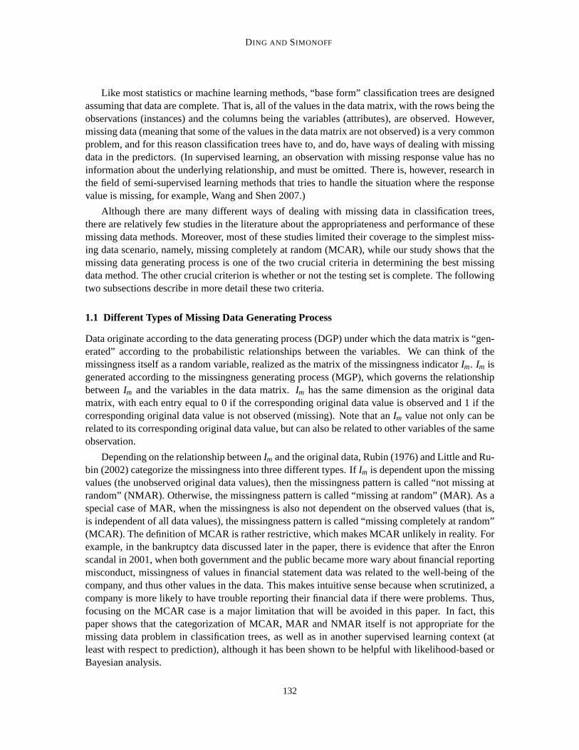
In Figure 1, the plot on the left is a scatter plot of relative accuracy versus missing rate foreach Monte Carlo replication for the complete case method when the MGP depends on the responsevariable. The lower bound is clearly shown. We can see that when the missing rate is high, thelower bound can reduce to almost zero (implying that not only relative accuracy, but accuracy itself,can approach zero). This perhaps somewhat counterintuitive result can occur in the following way.Imagine the extreme case where almost all cases are positive and (virtually)all of the positive caseshave missing predictor value at the training phase; in this situation the resultantrule will be toclassify everything as negative. When this rule is applied to a complete testing set with almost allpositive cases, the accuracy will be almost zero. The graph on the rightis the quantile version of thescatter plot on the left. The lines shown in the quantile plot are the theoretical lower bound, the 10th,20th, 30th, 40th and 50th percentile lines from the lowest to the highest. Higher percentile lines arethe same as the 50th percentile (median) line, which is already the horizontal lineatRelAcc= 1. Thepercentile lines are constructed by connecting the corresponding percentiles in a moving window

138


Figure 1: Scatter plot and the corresponding quantile plot of the complete testing setRelAccvs.missing rate of the complete case method when the MGP is dependent on the responsevariable. Recall that “∗∗Y” means the MGP is conditionally dependent on the responsevariable but no restriction on the relationship between the MGP and other variables, miss-ing or observed, is assumed. Each point in the scatter plot represents theresult on one ofthe simulated data tables.

of data from the left to the right. Due to space limitations, we do not show quantileplots of othermissing data methods and/or under different scenarios, but in all of the other plots, the quantile linesare all higher (that is, the quantile plot in Figure 1 shows the worst case scenario). The plots showthat the missing data problem, when the missing rate is not too high, may not be as serious as wemight have thought. For example, when 40% of the observations contain missing data, 80% of thetime the expected relative accuracy is higher than 90%, and 90% of the time the expected relativeaccuracy is higher than 80%.

3.1.2 WHEN THE TEST SET HAS M ISSING VALUES

Theorem 6 Separate Class: In 2×2 data tables, if missing values occur in both the training setand the testing set, then the separate class method achieves the best possible performance.

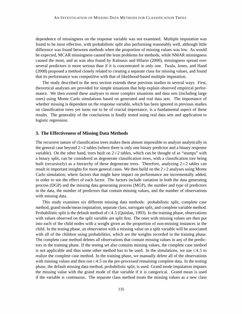
In the Monte Carlo simulation of the 2× 2 tables, the head-to-head comparison between theseparate class method and other missing data methods confirmed the uniform dominance of the sep-arate class when the test set also contains missing values, regardless whether the MGP is dependenton the response variable or not. However, as shown in Figure 2, when the MGP is independent ofthe response variable, separate class never performances better thanthe performance on the originalfull data, indicated by relative accuracies less than one. This means that separate class is not gainingfrom the missingness. On the other hand, when the MGP is dependent on theresponse variable, afairly large percentage of the time the relative accuracy of the separate class method is larger thanone (the quantiles shown are from the 10th to the 90th percentile with increment10 percent). Thismeans that trees based on the separate class method can improve on predictive performance com-pared to the situation where there are no missing data. Our simulations show thatother methodscan also gain from the missingness when the MGP is dependent on the response variable, but not asfrequently as the separate class method and the gains are in general not as large. We follow up onthis behavior in more detail in the next section, but the simple explanation is that since missingnessdepends on the response variable, the tree algorithm can use the presence of missing data in an ob-servation to improve prediction of the response for that observation. Duda, Hart, and Stork (2001)and Hand (1997) briefly mentioned this possibility in the classification context, but did not give any

139

DING AND SIMONOFF

Figure 2: Scatter plot of the separate class method with incomplete testing set. Each point in thescatter plot represents the result on one of the simulated data tables.

supporting evidence. Theorem 6 makes a fairly strong statement in the simple situation, and it willbe seen to be strongly indicative of the results in more general cases.

3.2 Monte Carlo Simulations of General Data Sets

In this section extensions of the simulations in the last section are summarized.

3.2.1 AN OVERVIEW OF THE SIMULATION

The following simulations are carried out.

1. 2×2 tables, missing values occur in the only predictor.

2. Up to seven binary predictors, missing values occur in only one predictor.

3. Eight binary predictors, missing values occur in two of them.

4. Twelve binary predictors, missing values occur in six of them.

5. Eight continuous predictors, missing values occur in two of them.

6. Twelve continuous predictors, missing values occur in six of them.

Two different scenarios of each of the last four simulations listed above were performed. Inthe first scenario, the six complete predictors are all independent of the missing ones, while in thesecond scenario three of the six complete predictors are related to the missingones. Therefore, tensimulations were done in total.

In each of the simulations, 5000 sets of DGPs are simulated in order to cover awide range ofdifferent-structured data sets so that a generalizable inference from the simulation is possible. For

140


In−sample accuracy

In−sample accuracy

Dens

ity

0.6 0.7 0.8 0.9 1.0

0.0

1.0

2.0

3.0

Out−of−sample accuracy

Out−of−sample accuracy

Dens

ity

0.5 0.6 0.7 0.8 0.9 1.0

0.0

1.0

2.0

3.0

In−sample AUC

In−sample AUC

Dens

ity

0.5 0.6 0.7 0.8 0.9 1.0

01

23

4

Out−of−sample AUC

Out−of−sample AUC

Dens

ity

0.5 0.6 0.7 0.8 0.9

04

8

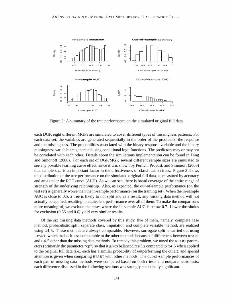
Figure 3: A summary of the tree performance on the simulated original full data.

each DGP, eight different MGPs are simulated to cover different types of missingness patterns. Foreach data set, the variables are generated sequentially in the order of the predictors, the responseand the missingness. The probabilities associated with the binary response variable and the binarymissingness variable are generated using conditional logit functions. Thepredictors may or may notbe correlated with each other. Details about the simulations implementation can be found in Dingand Simonoff (2008). For each set of DGP/MGP, several different sample sizes are simulated tosee any possible learning curve effect, since it was shown by Perlich, Provost, and Simonoff (2003)that sample size is an important factor in the effectiveness of classification trees. Figure 3 showsthe distribution of the tree performance on the simulated original full data, as measured by accuracyand area under the ROC curve (AUC). As we can see, there is broad coverage of the entire range ofstrength of the underlying relationship. Also, as expected, the out-of-sample performance (on thetest set) is generally worse than the in-sample performance (on the training set). When the in-sampleAUC is close to 0.5, a tree is likely to not split and as a result, any missing data method will notactually be applied, resulting in equivalent performance over all of them. To make the comparisonsmore meaningful, we exclude the cases where the in-sample AUC is below 0.7. Lower thresholdsfor exclusion (0.55 and 0.6) yield very similar results.

Of the six missing data methods covered by this study, five of them, namely, complete casemethod, probabilistic split, separate class, imputation and complete variable method, are realizedusingC4.5. These methods are always comparable. However, surrogate splitis carried out usingRPART, which makes it less comparable to the other methods because of differences betweenRPART

andC4.5 other than the missing data methods. To remedy this problem, we tuned theRPARTparam-eters (primarily the parameter “cp”) so that it gives balanced results compared toC4.5 when appliedto the original full data (i.e., each has a similar probability of outperforming the other), and specialattention is given when comparingRPART with other methods. The out-of-sample performances ofeach pair of missing data methods were compared based on botht-tests and nonparametric tests;each difference discussed in the following sections was strongly statisticallysignificant.

141

DING AND SIMONOFF

PP P

100 500 2000 10000

020

4060

80

− − −

Sample size

Winn

ing pc

t of e

ach m

ethod

C

CC

S S SM MMT

T T

D DD

P

PP

100 500 2000 10000

020

4060

80

− − Y

Sample size

Winn

ing pc

t of e

ach m

ethod

CC

CS S SM M MT

TT

D DD

PP P

100 500 2000 10000

020

4060

80

− X −

Sample size

Winn

ing pc

t of e

ach m

ethod

CC

C

SS SM M

MTT

T

D DD

P

PP

100 500 2000 10000

020

4060

80

− X Y

Sample size

Winn

ing pc

t of e

ach m

ethod

CC

CS S SM M MT

TT

D DD

PP P

100 500 2000 10000

020

4060

80

M − −

Sample size

Winn

ing pc

t of e

ach m

ethod

CC

CS S SM M

MTT T

D DD

P

P

P

100 500 2000 10000

020

4060

80

M − Y

Sample size

Winn

ing pc

t of e

ach m

ethod

CC

CS S SM M M

TT

T

D DD

PP P

100 500 2000 10000

020

4060

80

M X −

Sample size

Winn

ing pc

t of e

ach m

ethod

CC

CS S SM M MT

TT

D DD

P

P

P

100 500 2000 10000

020

4060

80

M X Y

Sample size

Winn

ing pc

t of e

ach m

ethod

CC

CS S SM M M

TT

T

D DD

Figure 4: A summary of the order of six missing data methods when tested on a new completetesting set. The Y axis is the percentage of times each method is the best (including beingtied with other methods; therefore the percentages do not sum up to one).

3.2.2 THE TWO FACTORS THAT DETERMINE THE PERFORMANCE OFDIFFERENTM ISSING

DATA METHODS

The simulations make clear that the dependence relationship between the missingness and the re-sponse variable is the most informative factor in differentiating different missing data methods, andthus is most helpful in determining the appropriateness of the methods. This can be clearly seen inFigures 4 and 5 (these figures refer to the case with twelve continuous predictors, six of which aresubject to missing values, but results for other situations were broadly similar). The left column in

142


PP

P

100 500 2000 10000

020

4060

80

− − −

Sample size

Winn

ing pc

t of e

ach m

ethod

C

CC

S S SM MMT

T T

D DD

P PP

100 500 2000 10000

020

4060

80

− − Y

Sample size

Winn

ing pc

t of e

ach m

ethod

CC

C

SS

S

M M MT

T TD D

D

PP P

100 500 2000 10000

020

4060

80

− X −

Sample size

Winn

ing pc

t of e

ach m

ethod

C

CC

S S SM MM

T TT

D DD P P

P

100 500 2000 10000

020

4060

80

− X Y

Sample size

Winn

ing pc

t of e

ach m

ethod

CC

C

SS

S

M M MT

T TD D

D

PP P

100 500 2000 10000

020

4060

80

M − −

Sample size

Winn

ing pc

t of e

ach m

ethod

CC

C

S S SM MMT

TT

D DD P P

P

100 500 2000 10000

020

4060

80

M − Y

Sample size

Winn

ing pc

t of e

ach m

ethod

CC

C

S

S

S

M M MT

T TD D

D

PP P

100 500 2000 10000

020

4060

80

M X −

Sample size

Winn

ing pc

t of e

ach m

ethod

CC

C

S S SM M MTT T

DD

D P PP

100 500 2000 10000

020

4060

80

M X Y

Sample size

Winn

ing pc

t of e

ach m

ethod

CC

C

S

S

S

M M MT

T TD D

D

Figure 5: A summary of the order of six missing data methods when tested on a new incompletetesting set. The Y axis is the percentage of times each method is the best (including beingtied with other methods).

the pictures shows the results when the missingness is independent of the response variable and theright column shows the results when the missingness is dependent on the response variable. We cansee that there are clear differences between the two columns, but within each column there is essen-tially no difference. This also says the categorization of MCAR/MAR/NMAR (which is based uponthe dependence relationship between the missingness and missing values, and does not distinguishthe dependence of the missingness on otherXs and onY) is not helpful in this context.

143

DING AND SIMONOFF

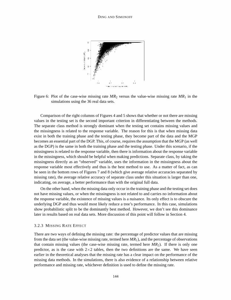
Figure 6: Plot of the case-wise missing rateMR2 versus the value-wise missing rateMR1 in thesimulations using the 36 real data sets.

Comparison of the right columns of Figures 4 and 5 shows that whether or not there are missingvalues in the testing set is the second important criterion in differentiating between the methods.The separate class method is strongly dominant when the testing set contains missing values andthe missingness is related to the response variable. The reason for this is that when missing dataexist in both the training phase and the testing phase, they become part of thedata and the MGPbecomes an essential part of the DGP. This, of course, requires the assumption that the MGP (as wellas the DGP) is the same in both the training phase and the testing phase. Under this scenario, if themissingness is related to the response variable, then there is information about the response variablein the missingness, which should be helpful when making predictions. Separate class, by taking themissingness directly as an “observed” variable, uses the information in the missingness about theresponse variable most effectively and thus is the best method to use. As amatter of fact, as canbe seen in the bottom rows of Figures 7 and 8 (which give average relative accuracies separated bymissing rate), the average relative accuracy of separate class under this situation is larger than one,indicating, on average, a better performance than with the original full data.

On the other hand, when the missing data only occur in the training phase and the testing set doesnot have missing values, or when the missingness is not related to and carries no information aboutthe response variable, the existence of missing values is a nuisance. Its only effect is to obscure theunderlying DGP and thus would most likely reduce a tree’s performance. In this case, simulationsshow probabilistic split to be the dominantly best method. However, we don’t see this dominancelater in results based on real data sets. More discussion of this point will follow in Section 4.

3.2.3 MISSING RATE EFFECT

There are two ways of defining the missing rate: the percentage of predictor values that are missingfrom the data set (the value-wise missing rate, termed hereMR1), and the percentage of observationsthat contain missing values (the case-wise missing rate, termed hereMR2). If there is only onepredictor, as is the case with 2×2 tables, then the two definitions are the same. We have seenearlier in the theoretical analyses that the missing rate has a clear impact on theperformance of themissing data methods. In the simulations, there is also evidence of a relationship between relativeperformance and missing rate, whichever definition is used to define the missing rate.

144


P PP

100 500 2000 10000

020

4060

8010

0

Winning Pct / MGP: MXY / MR1<0.15

Sample size

Winn

ing pc

t of e

ach m

ethod

C

CC

S

S

S

MM M

TT

T

DD D

P PP

100 500 2000 10000

020

4060

8010

0

Winning Pct / MGP: MXY / 0.2<MR1<0.3

Sample size

Winn

ing pc

t of e

ach m

ethod

CC

C

S

S

S

M M M

TT T

DD

D

PP

P

100 500 2000 10000

020

4060

8010

0

Winning pct / MGP: MXY / MR1>0.35

Sample size

Winn

ing Pc

t of e

ach m

ethod

C

CC

S

S

S

M

M M

TT

TD D

D

P P P

100 500 2000 10000

0.70.8

0.91.0

1.11.2

Mean RelAcc / MGP: MXY / MR1<0.15

Sample size

Relat

ive Ac

curac

y

C C C

S S SM M MT T TD

D D

PP P

100 500 2000 10000

0.70.8

0.91.0

1.11.2

Mean RelAcc / MGP: MXY / 0.2<MR1<0.3

Sample size

Relat

ive Ac

curac

y

CC

C

SS S

MM

M

T T TD

D D

PP P

100 500 2000 10000

0.70.8

0.91.0

1.11.2

Mean RelAcc / MGP: MXY / MR1>0.35

Sample size

Relat

ive Ac

curac

y

C C

SS S

MM M

T T TD D D

Figure 7: A comparison of the low, median and high missing rate situations. The top row shows thecomparison in terms of winning percentage and the bottom row shows the comparison ofthe absolute performance of each missing data method.

Figure 6 shows the relationship betweenMR1 andMR2 in the simulations with 12 continuouspredictors and 6 of them with missing values. Notice that in this setting,MR1 is naturally between0 and 0.5 (since half of the predictors can have missing values).MR2 values are considerably largerthanMR1 values, as would be expected.

The simulations clearly show that the relative performance of different missing data methods isvery consistent regardless of the missing rate (see the top row of Figure 7). However, the bottomrow of Figure 7 shows that the absolute performance of the complete case method and the meanimputation method deteriorate as the missing rate gets higher. It also shows that separate classmethod performs best when the missing rate is neither too high or too low, although this effect isrelatively small. Interestingly, the relative accuracy of the other missing datamethods is very closeto one regardless of the missing rate, indicating that they can almost achieve the same accuracy asif the data are complete without missing values.

A final effect connected to missing rate relates to results in earlier papers (Kalousis and Hilario,2000; Twala, 2009) that suggested that missingness over several predictors is more problematic thanmissingness concentrated in a few predictors. This pattern was not evident here (e.g., in comparingthe results for 8 predictors with 2 having missing values to those for 12 predictors with 6 havingmissing values), but it should be noted that the comparisons here are based on relative performancebetween methods, not absolute performance. That is, even if absolute performance deteriorates inthe presence of missingness over multiple predictors, this is less important to the data analyst thanis relative performance between methods (since a method must be chosen),and with respect to thelatter criterion the observed patterns are reasonably stable.

145

DING AND SIMONOFF

P

PP

100 500 2000 5000

020

4060

8010

0

Winning pct / MGP: MXY / 0.55<Orig. AUC<0.6

Sample size

Winn

ing p

ct of

eac

h m

etho

d

C

CC

S

S

S

M

MM

TT

T

D

DD

PP

P

100 500 2000 5000

020

4060

8010

0

Winning pct / MGP: MXY / 0.7<Orig. AUC<0.8

Sample size

Winn

ing p

ct of

eac

h m

etho

d

CC

C

S

S

S

MM M

TT

T

DD D

P

PP

100 500 2000 5000

020

4060

8010

0

Winning pct / MGP: MXY / Orig. AUC>0.9

Sample size

Winn

ing p

ct of

eac

h m

etho

d

CC

C

S SS

M M M

TT

T

D

DD

P P P

100 500 2000 5000

0.7

0.8

0.9

1.0

1.1

1.2

Mean RelAcc / MGP: MXY / 0.55<Orig. AUC<0.6

Sample size

Relat

ive A

ccur

acy

C

C

C

S

S

M

M MTT

TD D D P P P

100 500 2000 5000

0.7

0.8

0.9

1.0

1.1

1.2

Mean RelAcc / MGP: MXY / 0.7<Orig. AUC<0.8

Sample size

Relat

ive A

ccur

acy

CC

C

SS S

MM

M

T T TD

D D

P P P

100 500 2000 5000

0.7

0.8

0.9

1.0

1.1

1.2

Mean RelAcc / MGP: MXY / Orig. AUC>0.9

Sample size

Relat

ive A

ccur

acy

C

CC

SS S

M M MT T TD D D

Figure 8: A comparison of the low, median and high original full data AUC situations. The toprow shows the comparison in terms of winning percentage and the bottom row shows thecomparison of the absolute performance of each missing data method.

3.2.4 THE IMPACT OF THEORIGINAL FULL DATA AUC

Figure 8 shows that the original full data AUC primarily has an impact on the performance ofseparate class method. When the original full data AUC is higher, the loss in information due tomissing values is less likely to be compensated by the information in the missingness,and thusseparate class method deteriorates in performance (see the bottom row of Figure 8). When theoriginal AUC is very high, although separate class still does a little better on average, it loses thedominance over the other methods.

Another observation is that the missing data methods other than separate classhave fairly stablerelative accuracy, with complete case and mean imputation consistently being thepoorest perform-ers (see the graphs in the bottom rows of both Figure 7 and Figure 8). Thisis true regardless ofthe AUC or the missing rate, even when the missingness does not depend on the response variableand there are no missing data in the testing set where, in theory, the complete case method caneventually recover the DGP.

4. Performance On Real Data Sets

In this section, we show that most of the previously described results hold when using real datasets. Moreover, we propose a method of determining the best missing data method to use whenanalyzing a real data set. Unlike in the previous sections, in these simulations based on real data,default settings ofC4.5 are used andRPART is tuned (primarily using its parameter “cp”) to getsimilar performance on the original full data asC4.5. Therefore, in particular, the effect of pruningis present. In Section 4.1, we show the results on 36 data sets that were originally complete. InSection 4.2, we propose a way to determine the best missing data method to use when facing real

146


Missingness is related toMissing Observed Responsevalues Predictors Variable LR Three-LetterNo No No MCAR −−−

No No Yes MAR −−YYes No No NMAR M −−

Table 2: Three missingness patterns used in simulations based on real data sets. The LR columnshows the categorization according to Rubin (1976) and Little and Rubin (2002). TheThree-Letter column shows the categorization used in this paper.

data sets that contain missing values (since in that case the true missingness generating process isnot known by the data analyst).

4.1 Results on Real Data Sets with Simulated Missing Values

The same 36 data sets as in Perlich, Provost, and Simonoff (2003) are used here (except for Cover-type and Patent, which are too big forRPART to handle; in those cases a random subset of 100,000observations for each of them was used as the “true” underlying data set). They are either completeor were made complete by Perlich et al. (2003). Missing values with different missingness patternswere generated for the purpose of this study. According to the earlier results, the only importantfactor in the missingness generating process is the relationship between the missingness and theresponse variable. Therefore, two missingness patterns are included.In one of them, missingness isindependent of all of the variables (including the response variable). In the other one, missingness isrelated to the response variable, but independent of all of the predictors. These two missingness pat-terns can be categorized as missing completely at random (MCAR) and missingat random (MAR),respectively. To account for this categorization of MGPs, the third type of missingness, not missingat random (NMAR), is also included. In the NMAR case, missingness is madedependent upon themissing values but not on the response variable (see Table 2). To maximize the possible effect ofmissing values, the first split variable of the original full data is chosen as the variable that containsmissing values. It can be either numeric or categorical (binary or multi-categorical). Ten new datasets with missing values are generated for each combination of data set, training set size, and miss-ingness pattern combination, with the missing rate chosen randomly for each. The performance ofthe missing data methods is measured out-of-sample, on a hold out test sample.

The same six missing data methods, namely, the complete case method, the complete vari-able method, probabilistic split, grand mode/mean imputation, surrogate split and the separate classmethod are applied. All of them are realized usingC4.5 except for surrogate split, which is realizedusingRPART. C4.5 is run with its default settings. To make surrogate split comparable to the othermissing data methods, theRPARTparameters are tuned for each data set and each sample size so thatRPART andC4.5 have comparable in sample performance on the original full data (by comparableperformance we mean the average in sample original full data accuracies are similar to each other).

147

DING AND SIMONOFF

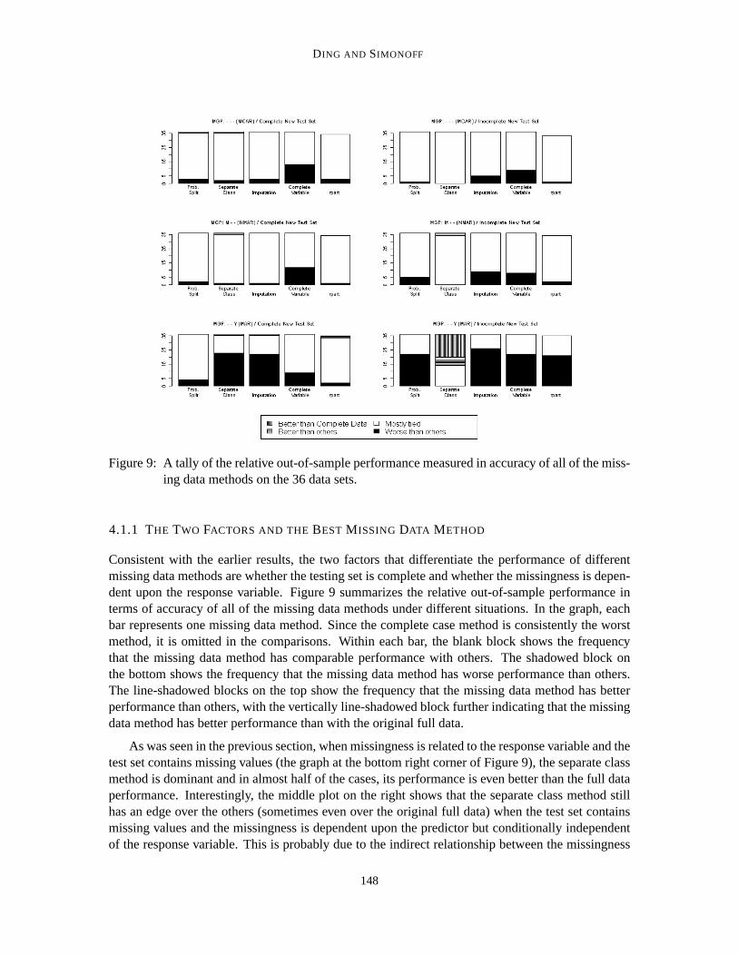
Figure 9: A tally of the relative out-of-sample performance measured in accuracy of all of the miss-ing data methods on the 36 data sets.

4.1.1 THE TWO FACTORS AND THEBEST M ISSING DATA METHOD

Consistent with the earlier results, the two factors that differentiate the performance of differentmissing data methods are whether the testing set is complete and whether the missingness is depen-dent upon the response variable. Figure 9 summarizes the relative out-of-sample performance interms of accuracy of all of the missing data methods under different situations. In the graph, eachbar represents one missing data method. Since the complete case method is consistently the worstmethod, it is omitted in the comparisons. Within each bar, the blank block shows thefrequencythat the missing data method has comparable performance with others. The shadowed block onthe bottom shows the frequency that the missing data method has worse performance than others.The line-shadowed blocks on the top show the frequency that the missing data method has betterperformance than others, with the vertically line-shadowed block further indicating that the missingdata method has better performance than with the original full data.

As was seen in the previous section, when missingness is related to the response variable and thetest set contains missing values (the graph at the bottom right corner of Figure 9), the separate classmethod is dominant and in almost half of the cases, its performance is even better than the full dataperformance. Interestingly, the middle plot on the right shows that the separate class method stillhas an edge over the others (sometimes even over the original full data) when the test set containsmissing values and the missingness is dependent upon the predictor but conditionally independentof the response variable. This is probably due to the indirect relationship between the missingness

148


and the response variable because both the missingness and the response variable are related to thepredictor.

However, the dominance of probabilistic split is not observed in these realdata sets. One pos-sible reason could be the effect of pruning, which is used in these real data sets. The other twomethods realized usingC4.5 (imputation and separate class) both work with “filled-in” data sets,while probabilistic split takes the missing values as-is. Given this, we speculatethat the brancheswith missing values are more likely to be pruned under probabilistic split, which causes it to losepredictive power. Another possible reason could be the competition from surrogate split, which isrealized usingRPART. Although we tried to tuneRPART for each data set and each sample size,RPARTandC4.5 are still two different algorithms. Different features ofRPARTandC4.5, other thanthe missing data methods, may causeRPART to outperformC4.5. Complete variable method per-forms a bit worse than the others, presumably because in these simulations theinitial split variableon the full data was used as the variable with missing values.

In addition to accuracy, AUC was also tested as an alternative performance measure. We alsoexamined the use of bagging (bootstrap aggregating) to reduce the variability of classification trees(discussion of bagging can be found in many sources, for example, Hastie et al. 2001). The learningcurve effect (that is, the relationship between effectiveness and sample size) is also examined. Wesee patterns consistent with those in the simulated data sets. That is, the relative performance of themissing data methods is fairly consistent across different sample sizes.

4.1.2 THE EFFECT OFM ISSING RATE

Figure 10 shows the distribution of the generated missing rates in these simulations. Recall thatmissing values occur in one variable, so this missing rate is the percentage of observations that havemissing values, that is,MR2 as defined earlier. Figure 11 shows a comparison between the case whenthe missing rate is low (MR2 < 0.2) and the case when the missing rate is high (MR2 > 0.8). Forbrevity, only the result when the MGP is dependent on the response variable is shown; differencesbetween the low and high missing rate situations for other MGP’s are similar. Since the missingrate is chosen at random, some of the original data sets do not have any generated data sets withsimulated missing values with low missing rate, while for others we do not have anywith highmissing rate, which accounts for the “no data” category in the figures. Also, when the missing rateis high, the complete case method is obviously much worse than other missing data methods, and istherefore omitted from the comparison in that situation.

By comparing the graphs in Figures 11 with the corresponding ones in Figure 9, we can seesome of the effects of missing rate. First, when the missing rate is lower than 0.2,the complete casemethod has comparable performance to other methods other than the complete variable method.This is unsurprising, as in this situation the complete case method does not lose much informationfrom omitted observations. Secondly, the complete variable method has the worst performancewhen the missing rate is low, presumably (as noted earlier) because the complete variable methodomits the most important explanatory variable in these simulations.

Moreover, in both the low and high missing rate cases, when the missingness depends on theresponse and the testing set is incomplete, the dominance of the separate class is not as strong as itis in Figure 9. This indicates that separate class works best when the missingrate is moderate. Ifthe missing rate is too low, there might not be enough observations in the category of “missing” forthe separate class method to be as effective. On the other hand, if the missingrate is very high, the

149

DING AND SIMONOFF

Distribution of missing rates in the simulation on 36 real data sets

Missing Rate

Den

sity

0.0 0.2 0.4 0.6 0.8 1.0

0.0

0.2

0.4

0.6

0.8

1.0

1.2

1.4

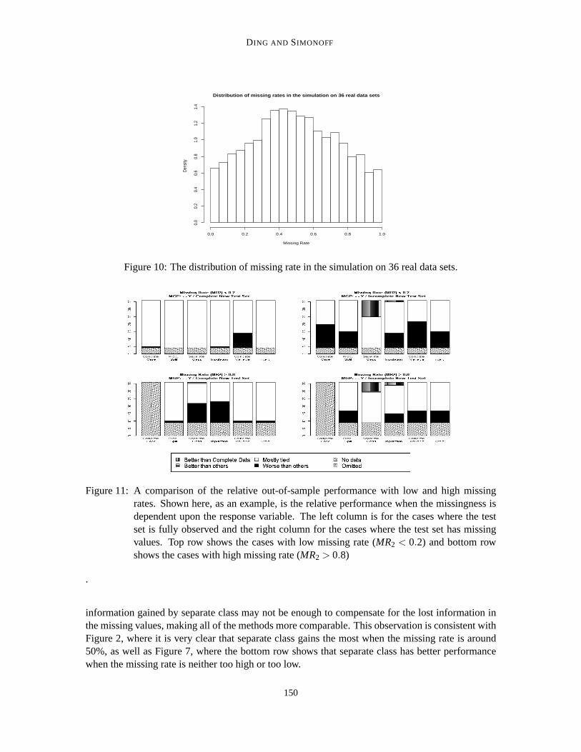
Figure 10: The distribution of missing rate in the simulation on 36 real data sets.

Figure 11: A comparison of the relative out-of-sample performance with lowand high missingrates. Shown here, as an example, is the relative performance when the missingness isdependent upon the response variable. The left column is for the caseswhere the testset is fully observed and the right column for the cases where the test sethas missingvalues. Top row shows the cases with low missing rate (MR2 < 0.2) and bottom rowshows the cases with high missing rate (MR2 > 0.8)

.

information gained by separate class may not be enough to compensate for the lost information inthe missing values, making all of the methods more comparable. This observationis consistent withFigure 2, where it is very clear that separate class gains the most when themissing rate is around50%, as well as Figure 7, where the bottom row shows that separate classhas better performancewhen the missing rate is neither too high or too low.

150


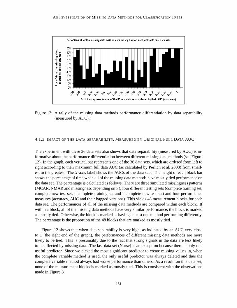
Figure 12: A tally of the missing data methods performance differentiation by data separability(measured by AUC).

4.1.3 IMPACT OF THEDATA SEPARABILITY, MEASURED BY ORIGINAL FULL DATA AUC

The experiment with these 36 data sets also shows that data separability (measured by AUC) is in-formative about the performance differentiation between different missing data methods (see Figure12). In the graph, each vertical bar represents one of the 36 data sets, which are ordered from left toright according to their maximum full data AUC (as calculated by Perlich et al. 2003) from small-est to the greatest. TheX-axis label shows the AUCs of the data sets. The height of each black barshows the percentage of time when all of the missing data methods have mostly tied performance onthe data set. The percentage is calculated as follows. There are three simulated missingness patterns(MCAR, NMAR and missingness depending onY), four different testing sets (complete training set,complete new test set, incomplete training set and incomplete new test set) and four performancemeasures (accuracy, AUC and their bagged versions). This yields 48 measurement blocks for eachdata set. The performances of all of the missing data methods are compared within each block. Ifwithin a block, all of the missing data methods have very similar performance, theblock is markedas mostly tied. Otherwise, the block is marked as having at least one method performing differently.The percentage is the proportion of the 48 blocks that are marked as mostly tied.

Figure 12 shows that when data separability is very high, as indicated by anAUC very closeto 1 (the right end of the graph), the performances of different missing data methods are morelikely to be tied. This is presumably due to the fact that strong signals in the data are less likelyto be affected by missing data. The last data set (Nurse) is an exception because there is only oneuseful predictor. Since we picked the most significant predictor to createmissing values in, whenthe complete variable method is used, the only useful predictor was always deleted and thus thecomplete variable method always had worse performance than others. As aresult, on this data set,none of the measurement blocks is marked as mostly tied. This is consistent with the observationsmade in Figure 8.

151

DING AND SIMONOFF

4.2 A Real Data Set With Missing Values

We now present a real data example with naturally occurred missing values.In this example, wetry to model a company’s bankruptcy status given its key financial statementitems. The data areannual financial statement data and the predictions are sequential. That is, we build the tree on oneyear’s data and then test its performance on the following year’s data. For example, we build a treeon 1987’s data and test its performance on 1988’s data, then build a tree on 1988’s data and test iton 1989 data, and so on.

The data are retrieved from Compustat North America (a database of U.S. and Canadian funda-mental and market information on more than 24,000 active and inactive publiclyheld companies).Following Altman and Sabato (2005), twelve variables from the data base areused as potential pre-dictors: Current Assets, Current Liabilities, Assets, Sales, Operating Income Before Depreciation,Retained Earnings, Net Income, Operating Income After Depreciation, Working Capital, Liabili-ties, Stockholder’s Equity and year. The response variable, bankruptcy status, is determined usingtwo footnote variables, the footnote for Sales and the footnote for Assets.Companies with remarkscorresponding to “Reflects the adoption of fresh-start accounting upon emerging from Chapter 11bankruptcy” or “Company in bankruptcy or liquidation” are marked as bankruptcy. The data in-clude all active companies, and span 19 years from 1987 to 2005. There are 177560 observationsin the original retrieved data, but 76504 of the observations have no dataexcept for the companyidentifications, and are removed from the data set, resulting in 99056 observations. There are 19238(19.4%) observations containing missing values and there are 56820 (4.8%) missing data values.

According to the results in Sections 3 and 4.1, there are two criteria that differentiate the per-formance of different missing data methods, that is, whether or not there are missing values in thetesting set and whether or not the missingness depends on the response variable. In the bankruptcydata, there are missing values in every year’s data, and thus missing valuesin each testing data set.To assess the dependence of the missingness on the response variable,the following test is carriedout. First, we define twelve new binary missingness indicators corresponding to the original twelvepredictors. Each indicator takes on value 1 if the original value for the associated variable is missingand 0 if the original value is observed for that observation. We then build atree for each year’s datausing the indicators as the predictors and the original response variable,the bankruptcy status, asthe response variable. From 1987 to 2000, the tree makes no split, indicatingthe tree algorithm isnot able to establish a relationship between the missingness and the responsevariable. From 2001to 2005, the classification tree consistently splits on the missingness indicators of Sales and Re-tained Earnings. This indicates that the missingness of these predictors hasinformation about theresponse variable in these years, and the MGP across the years is fairlyconsistent in missingness insales and retained earnings being related to bankruptcy status. However, the AUC values calculatedfrom the trees built with the missingness indicators are not very high, all being between 0.5 and 0.6.Therefore, the relationship is not a very strong one.

Given these observations and the fact that the sample sizes are fairly large, we would makethe following propositions based on our earlier conclusions. First, from 1988 to 2001 (since thetree tested on 2001 data is built on 2000 data), different missing data methodsshould have simi-lar performance, with no clear winners. However, from year 2002 to year 2005, the separate classmethod should have better performance than the others (but perhaps notmuch better since the rela-tionship between missingness and the response is not very strong). The actual relative performanceof different missing data methods is shown in Figure 13. Since surrogate split is realized using

152


rpart accuracy, missingness indep of response

year

Accu

racy

1988 1990 1992 1994 1996 1998 2000

0.98

00.

990

1.00

0

C4.5 accuracy, missingness indep of response

year

Accu

racy

1988 1990 1992 1994 1996 1998 2000

0.98

00.

990

1.00

0

rpart accuracy, missingness dep on response

year

Accu

racy

2002 2003 2004 2005

0.98

00.

990

1.00

0

C4.5 accuracy, missingness dep on response

year

Accu

racy

2002 2003 2004 2005

0.98

00.

990

1.00

0rpart TP, missingness indep of response

year

True

Pos

itive

Rat

e

1988 1990 1992 1994 1996 1998 2000

0.0

0.1

0.2

0.3

0.4

0.5

C4.5 TP, missingness indep of response

year

True

Pos

itive

Rat

e

1988 1990 1992 1994 1996 1998 2000

0.0

0.1

0.2

0.3

0.4

0.5

rpart TP, missingness dep on response

year

True

Pos

itive

Rat

e

2002 2003 2004 2005

0.0

0.1

0.2

0.3

0.4

0.5

C4.5 TP, missingness dep on response

year

True

Pos

itive

Rat

e

2002 2003 2004 2005

0.0

0.1

0.2

0.3

0.4

0.5

Figure 13: The relative performance of all of the missing data methods on thebankruptcy data.The left column gives methods usingRPART (and includes all of the methods exceptfor probabilistic split) and the right column gives methods usingC4.5 (and includes allof the methods except for surrogate split). The top rows are performance in terms ofaccuracy while the bottom rows are in terms of true positive rate.

RPART while probabilistic split is realized usingC4.5, we run all of the other methods using bothRPART andC4.5 so that we can compare both surrogate split and probabilistic split with allof theother methods. In Figure 13, the plots on the left are the results fromRPART, which include all of

153

DING AND SIMONOFF

the missing data methods except for probabilistic split. The plots on the right arethe results fromC4.5, which include all of the missing data methods except for surrogate split.The performancesof methods common to both plots are slightly different because of differences betweenC4.5 andRPART in splitting and pruning rules. Both the accuracy and the true positive rates are shown. Sincethe number of actual bankruptcy cases in the data is small, the accuracy is always very high. Thetrue positive rate is defined as

TP=Number of correctly predicted bankruptcy cases

Actual number of bankruptcy cases.

The graphs in the first and the second rows are for accuracies, with thefirst row for the first timeperiod from 1988 to 2001 and the second row for the second time period from 2002 to 2005. Thegraphs in the third and the fourth rows are for true positive rates, with the third row for the first timeperiod from 1988 to 2001 and the fourth row for the second time period from 2002 to 2005. It isapparent that in the first time period, there are no clear winners. However, in the second time period,separate class is a little better than the others, in line with expectations.

5. Extension To Logistic Regression

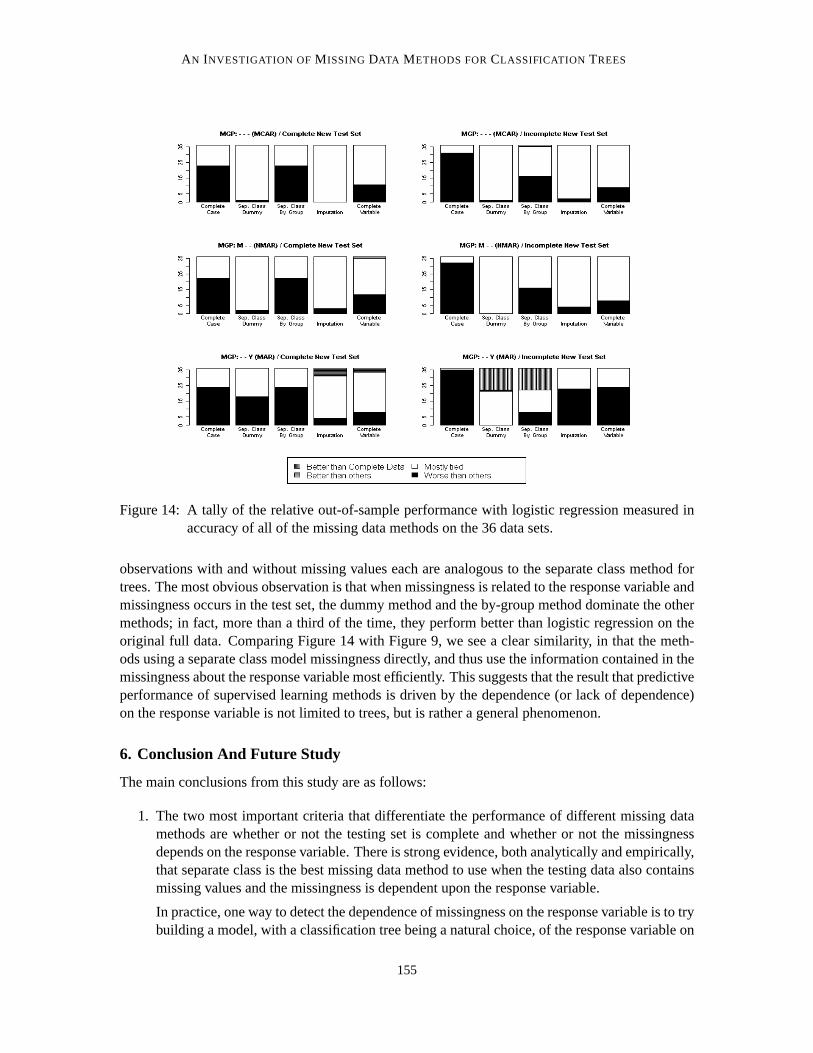
One obvious observation from this study is that when missing values occur inboth the model build-ing and model application stages, it should be considered as part of the data generating processrather than a separate mechanism. That is, taking the missingness into consideration can improvepredictive performance, sometimes significantly. This should also apply to other supervised learn-ing methodologies, non-parametric or parametric, when predictive performance is concerned. Wepresent here the results from a real data analysis study involving logistic regression, similar to theone presented in Section 4.1. Missing values are generated the same way asin Section 4.1 andthen logistic regression models (without variable selection) with different ways of handling missingdata are applied to those data sets. Finally a tally is made on the relative performances of differentmissing data methods. Results measured in accuracy, bagged accuracy, AUC and bagged AUC arealmost identical to each other; results in terms of accuracy are shown in Figure 14.

Included in the study are five ways of handling missing data: using only complete cases (com-plete case method), including a missingness dummy variable in the explanatory variable (dummymethod, sometimes called the missing-indicator method),1 building separate models for data withvalues missing and data without missing values (by-group method),2 imputing missing values withgrand mean/mode (imputation method), and only using predictors without missing values (completevariable method). Note that the methods using a dummy variable and building separate models for

1. If explanatory variableX1 has missing values, then we create a missingness dummy variableM1 that has value 1 ifX1is observed and 0 otherwise. ThenM1 andX1 ∗M1 are both used as explanatory variables. The result of this set-upis that the effect ofX1 is fit on the observations withX1 observed but a single mean value is fit to the observationswith X1 missing. All of the observations, with or withoutX1 values, have the same coefficients for all of the otherexplanatory variables. Jones (1996) showed that this method can result in biased coefficient estimates in regressionmodeling, but did not address the question of predictive accuracy thatis the focus here.

2. The biggest difference between the by-group method and the dummymethod is whether the explanatory variables,other than the one containing missing values, have different coefficientsor not. The by-group method fits two separatemodels to observations with and without missing values. Therefore, evenif an explanatory variable is fully observed,its coefficient would most likely be different for fully observed observations and for observations with missing values.The dummy method, on the other hand, fits a single model to the entire data set so that variables that are fully observedwill have the same coefficients whether an observation has missing valuesor not.

154


Figure 14: A tally of the relative out-of-sample performance with logistic regression measured inaccuracy of all of the missing data methods on the 36 data sets.

observations with and without missing values each are analogous to the separate class method fortrees. The most obvious observation is that when missingness is related to theresponse variable andmissingness occurs in the test set, the dummy method and the by-group method dominate the othermethods; in fact, more than a third of the time, they perform better than logistic regression on theoriginal full data. Comparing Figure 14 with Figure 9, we see a clear similarity,in that the meth-ods using a separate class model missingness directly, and thus use the information contained in themissingness about the response variable most efficiently. This suggests that the result that predictiveperformance of supervised learning methods is driven by the dependence (or lack of dependence)on the response variable is not limited to trees, but is rather a general phenomenon.

6. Conclusion And Future Study

The main conclusions from this study are as follows:

1. The two most important criteria that differentiate the performance of different missing datamethods are whether or not the testing set is complete and whether or not the missingnessdepends on the response variable. There is strong evidence, both analytically and empirically,that separate class is the best missing data method to use when the testing data also containsmissing values and the missingness is dependent upon the response variable.

In practice, one way to detect the dependence of missingness on the response variable is to trybuilding a model, with a classification tree being a natural choice, of the response variable on

155

DING AND SIMONOFF

the missingness indicators (which equals to 1 if the corresponding original value is missingand 0 otherwise). If such a model supports a relationship, then it is an indication that themissingness is related to the response variable.

2. The performance of classification trees is on average not too negatively affected by missingvalues, except for the complete case method and the mean imputation method, which aresensitive to different missing rates. Separate class tend to perform betterwhen the missingrate is neither too high nor too low, trading off between information loss due to missing valuesand information gain from the informative MGP.

3. The original full data AUC has an impact on the performance of separate class method. Thehigher the original AUC, the more severe the information loss due to missing value, and thusrelatively the worse the performance of the separate class method.

The consistency of these results across the theoretical analyses, simulations from the artificial data,and simulations based on real data provides strong support for their general validity.

The findings here also have implications beyond analysis of the data at hand. For example, sincemissingness that is dependent on the response variable can actually improve predictive performance,it is clear that expending time, effort, and money to recover the missing valuesis potentially a poorway to allocate resources. Another interesting implication of these results is related to data disclo-sure limitation. It is clear that any masking of values must be done in a way that isindependent ofthe response variables of interest (or any predictors highly related to such variables), since otherwisedata disclosure using regression-type methods (Palley and Simonoff, 1987) could actually increase.

Classification trees are designed for the situation where the response variable is categorical, notjust binary; it would be interesting to see how these results carry over to that situation. Tree-basedmethodologies for the situation with a numerical response have also been developed (i.e., regressiontrees), and the problems of missing data occur in that context also. Investigating such trees wouldbe a natural extension of this paper. In this paper, we focused on baseform classification treesusingC4.5 andRPART, although bagging was included in the study. It would be worthwhile to seehow the performance of different missing data methods is affected by different tree features such asstopping and pruning or when techniques such as cross-validation, treeensembles, etc. are used.

Moreover, as was shown in Section 5, the relationship between the missingness and the responsevariable can be helpful in prediction when missingness occurs in both the training data and thetesting data in situations other than classification trees. This is very likely true for other supervisedlearning methods, and thus testing more learning methods would also be a natural extension to thisstudy.

Acknowledgments

The authors would like to thank Foster Provost for his helpful comments, which have helped us togreatly improve the quality of this paper. The authors also thank several anonymous referees forhelpful comments that greatly improved the presentation of results in the paper.

156


P(Y = 0|X = 0,with Missing Data) > T > TP(Y = 0|X = 1,with Missing Data) > T ≤ TP(Y=0|X=0) P(Y=0|X=1)

> T > T 1 P(X=0,Y=0)+P(X=1,Y=1)P(Y=0)

> T ≤ T P(Y=0)P(X=0,Y=0)+P(X=1,Y=1) 1

≤ T > T P(Y=0)P(X=0,Y=1)+P(X=1,Y=0)

P(X=0,Y=0)+P(X=1,Y=1)P(X=0,Y=1)+P(X=1,Y=0)

≤ T ≤ T P(Y=0)P(Y=1)

P(X=0,Y=0)+P(X=1,Y=1)P(Y=1)

P(Y = 0|X = 0,with Missing Data) ≤ T ≤ TP(Y = 0|X = 1,with Missing Data) > T ≤ TP(Y=0|X=0) P(Y=0|X=1)

> T > T P(X=0,Y=1)+P(X=1,Y=0)P(Y=0)

P(Y=1)P(Y=0)

> T ≤ T P(X=0,Y=1)+P(X=1,Y=0)P(X=0,Y=0)+P(X=1,Y=1)

P(Y=1)P(X=0,Y=0)+P(X=1,Y=1)

≤ T > T 1 P(Y=1)P(X=0,Y=1)+P(X=1,Y=0)

≤ T ≤ T P(X=0,Y=1)+P(X=1,Y=0)P(Y=1) 1

Table 3: RelAccof tree built on data with missing values and tested on the original full data setwhen there is no variation from true DGP

Appendix A. Proofs of the Theorems

The relative accuracy (RelAcc) when there are missing values in the training set but not in the testingset can be summarized into Table 3, whereT is the threshold value (an observation will be classifiedas class 0 if the predicted probability for it to be 0 is greater thanT). The value ofT reflects themisclassification cost. It is taken as 0.5 reflecting an equal misclassification cost. In Table 3, thecolumns show different rules given by the classification trees when thereare missing values, and therows show actual DGP’s. The entries are theRelAccvalues under different scenarios. For example,all of the entries on the diagonal are one’s because the rules given by the classification trees whenthere are missing values are the same as the true DGP’s and thus the accuracy achieved by the treesare the same with or without the missing values and thusRelAcc= 1. Cell (1,2), for example,shows that if the true DGP isP(Y = 0|X = 0) > T andP(Y = 0|X = 1) > T but the classificationtree gives ruleP(Y = 0|X = 0) > T andP(Y = 0|X = 1) ≤ T when there are missing values, thatis, P(Y = 0|X = 0,with missing value) > T andP(Y = 0|X = 1with missing value) ≤ T, then therelative accuracy is determined to be

P(X = 0,Y = 0)+P(X = 1,Y = 1)

P(Y = 0).

Proof of Theorem 1 : The expected performance of the complete case method when the missing-ness does not depend on the response variable and the testing set is complete.

Proof

First, we defineA as the case-wise missingness indicator which equals 1 if the observationcontains missing values in one or more of the predictors or 0 if the observationdoes not

157

DING AND SIMONOFF

contain missing values in any of the predictors.Y is the response variable andX is the vectorof the predictors.

If only the complete cases are used, ifP(Y|A = 0,X) = P(Y|X), then only the diagonal inTable 3 can be achieved, and thus there is no loss in accuracy.

This condition will be satisfied if and only if the MGP is conditionally independentof Y givenX, that is,P(A = 0|X,Y) = P(A = 0|X).

1. “P(Y|A = 0,X) = P(Y|X) ⇒ P(A = 0|X,Y) = P(A = 0|X)”

P(A=0|X,Y)= P(A=0,X,Y)P(X,Y)

=P(Y|A=0,X)P(A=0,X)P(X,Y)

=P(Y|X)P(A=0,X)P(Y|X)P(X)

=P(A = 0|X)

2. “P(Y|A = 0,X) = P(Y|X) ⇐ P(A = 0|X,Y) = P(A = 0|X)”

P(Y|A=0,X)= P(A=0,X,Y)P(A=0,X)

=P(A=0|X,Y)P(X,Y)P(A=0,X)

=P(A=0|X)P(X,Y)P(A=0|X)P(X)

=P(X,Y)P(X)

=P(Y|X)

Proof of Theorems 2 and 3 : The expected performance of the complete case method when themissingness depends on the response variable and the testing set is complete.

We first observe the following lemmas.

Lemma 7 For the partition defined by the tree built on the original full data (and not changedby missing values), let the kth section contain Pk proportion of data and within the partition,the majority class have proportion Pk

m j. Note that∑Kk=1Pk = 1, while the full data set accu-

racy, that is, the accuracy achievable with the full data set, is∑k PkPkm j.)

The rule for the kth section will be classifying it as the majority class of the section. Theimpact of missing data on its rule is to either leave it unchanged or make it classify the dataas the minority class instead of the majority class.

The smallest missing rate needed in kth section to change the rule is P(A = 1|k) = 2Pkm j−1,

where A is defined as in Theorem 1, that is, it is the case-wise indicator, which takes value1 if the observation contains missing value or 0 otherwise. If the rule is changed the loss inaccuracy within that section is2Pk

m j−1.

158


Proof

We assume the partition of the data is not changed by the missing values. The structure of thetrees need not to be the same because different trees may lead to the same partition of data.

For anyk, to make the rule of thekth section change, we need to observe more minority classcases than the majority ones within that section. To achieve this in the most efficient way,we only make the majority ones missing. Originally, there arePk

m j majorities and 1−Pkm j

minorities. Only when there arePkm j− (1−Pk

m j) = 2Pkm j−1 majorities missing will it become

less than the minorities, so this is the smallest missing rate we need to make the rule change.

After the rule is changed, only 1−Pkm j of the data, that is, the minorities, will be correctly

classified. Therefore, the loss in accuracy isPkm j− (1−Pk

m j) = 2Pkm j−1.

Lemma 8 For a given data set and the partition defined by the tree built on the full data set(which is not changed by the missing values), the largest loss in accuracy is∑k 2Pk

m j−1. The

smallest missing rate needed to achieve this is also∑k 2Pkm j−1.

Proof

The largest loss is achieved if and only if the rules are changed in every section of data in thepartition. The result then follows from Lemma 7.

Lemma 9 For a certain missing rate, say Pm, the largest effect it can have on the classifica-tion accuracy of any data that won’t be split is Pm itself.

In this case, the data set has its majority proportion Pm j =12(1+Pm).

Proof

Similar to the proof of Lemma 7, for missing values to have an impact on the classificationrule, it has to switch the order status of the majority and minority. To achieve this,it has tobe thatPm j− (1−Pm j) ≤ Pm. We know that once the rule is changed, the loss in accuracy isPm j − (1−Pm j). Therefore, the largest loss isPm when the equality holds. In this case, wehavePm j =

12(1+Pm).

We now prove Theorem 2.

Proof

For any data set, once it is partitioned and the partition is not changed by missing values,the rules in different sections of data are independent of each other, so we can look at themseparately.

159

DING AND SIMONOFF

Suppose the data are partitioned intoK segments, in which some contain missing data andthe others do not. LetK0 be the set of sections whose rules are changed by missing data andK1 be the set of all other sections. Also let thekth segment (k = 1. . .K) contain proportionPk

of the data. We have∑Kk=1Pk = 1.

Assume that thekth segment (k∈ K0) contains proportionPkm of missing data. Then we have

∑k∈K0

PkmPk ≤ Pm.

For thekth segment (k ∈ K0), by Lemma 9, the largest possible loss in accuracy isPkm and it

occurs if and only ifPkm j =

12(1+Pk

m). Therefore, the possible loss for the entire data set is

∑k∈K0

PkmPk ≤ Pm,

the largest loss being achieved when the equality holds. In that case, the rules in all of thecategories that contain missing values are changed and the maximum loss isPm.

We now prove Theorem 3.

Proof

Assuming the partitions of data are not changed by the missing values, we have

RelAcc =∑K

k=1Pkm jP

k−∑k∈K0(loss in accuracy inkth segment)

∑Kk=1Pk

m jPk

= 1−∑k∈K0

(loss in accuracy inkth segment)

∑Kk=1Pk

m jPk

= 1−∑k∈K0


∑k∈K0Pk

m jPk +∑k∈K1

Pkm jP

k

This is an increasing function of∑k∈K1Pk

m jPk in the denominator, which is independent of

other factors; setting it to zero minimize therelative accuracy, so

RelAcc ≤ 1−∑k∈K0


∑k∈K0Pk

m jPk

Denote the numerator∑k∈K0(loss in accuracy inkth segment) asa. Now, from the proof of

Theorem 2, the numeratora≤ Pm and the denominator∑k∈K0Pk

m jPk = 1

2(1+a). So,

RelAcc ≤ 1−a

12(1+a)

160


This is a decreasing function ofa and subject toa≤ Pm. Therefore, the minimumRelAccisachieved whena = Pm. This gives

RelAcc ≤ 1−Pm

12(1+Pm)

=1−Pm

1+Pm

Proof of Theorem 4 : Some properties of probabilistic split when the missingness does not dependon both the predictor and the response variable.

Proof

1. Part 1

• If the MGP is independent ofY givenX, that is,P(M|X,Y)= P(M|X) thenP(Y|M,X)=P(Y|X) by the proof of Theorem 1.The rules given by probabilistic split when there are missing values are as follows:

P(Y = 0|X = 0,Prob split)

= P(Y = 0|M = 0,X = 0)P(M = 0)+P(Y = 0|M = 1)P(M = 1)

= P(Y = 0|X = 0)P(M = 0)+P(Y = 0|M = 1)P(M = 1)

= P(Y = 0|X = 0)P(M = 0)

+[P(Y = 0,X = 0|M = 1)+P(Y = 0,X = 1|M = 1)]P(M = 1)

= P(Y = 0|X = 0)P(M = 0)

+[P(Y = 0|M = 1,X = 0)P(X = 0|M = 1)

+P(Y = 0|M = 1,X = 1)P(X = 1|M = 1)]P(M = 1)

= P(Y = 0|X = 0)P(M = 0)+ [P(Y = 0|X = 0)P(X = 0|M = 1)

+P(Y = 0|X = 1)P(X = 1|M = 1)]P(M = 1)

= P(Y = 0|X = 0)P(M = 0)+P(Y = 0|X = 0)P(M = 1,X = 0)

+P(Y = 0|X = 1)P(M = 1,X = 1)

= P(Y = 0|X = 0)[P(M = 0)+P(M = 1,X = 0)]

+P(Y = 0|X = 1)P(M = 1,X = 1)

and following the similar route, we can get


= P(Y = 0|X = 1)[P(M = 0)+P(M = 1,X = 1)]

+P(Y = 0|X = 0)P(M = 1,X = 0).

Note that

P(M = 0)+P(M = 1,X = 1)+P(M = 1,X = 0) = 1.

161

DING AND SIMONOFF

Therefore,


=P(M = 0|Y = 0)P(Y = 0|X = 0)P(M = 0)

P(M = 0|Y = 0)P(Y = 0|X = 0)+P(M = 0|Y = 1)P(Y = 1|X = 0)

−P(M = 0|Y = 0)P(Y = 0|X = 1)P(M = 0)

P(M = 0|Y = 0)P(Y = 0|X = 1)+P(M = 0|Y = 1)P(Y = 1|X = 1)

= [P(Y = 0|X = 0)P(M = 0|Y = 0)P(Y = 0|X = 1)

+P(Y = 0|X = 0)P(M = 0|Y = 1)P(Y = 1|X = 1)

−P(Y = 0|X = 1)P(M = 0|Y = 0)P(Y = 0|X = 0)

−P(Y = 0|X = 1)P(M = 0|Y = 1)P(Y = 1|X = 0)]P(M = 0|Y = 0)P(M = 0)

D1D2

= [P(Y = 0|X = 0)−P(Y = 0|X = 1)]P(M = 0|Y = 1)P(M = 0|Y = 0)P(M = 0)

D1D2

= [P(Y = 0|X = 0)−P(Y = 0|X = 1)]K

whereD1 = P(M = 0|Y = 0)P(Y = 0|X = 0)+P(M = 0|Y = 1)P(Y = 1|X = 0),

D2 = P(M = 0|Y = 0)P(Y = 0|X = 1)+P(M = 0|Y = 1)P(Y = 1|X = 1)

andK =

P(M = 0|Y = 1)P(M = 0|Y = 0)P(M = 0)

D1D2.

SinceK is always positive as long as there are differentY values observed, we cansee that the probabilistic split preserves the order of the conditional probability ofY givenX.Now, without loss of generality, assumeP(Y = 0|X = 0,Prob split) > T andP(Y =0|X = 1,Prob split) < T. It follows thatP(Y = 0|X = 0) > P(Y = 0|X = 1) becauseprobabilistic split preserves the correct order. There are three possibilities:

(a) P(Y = 0|X = 0) > T > P(Y = 0|X = 1)

(b) T > P(Y = 0|X = 0) > P(Y = 0|X = 1)

(c) P(Y = 0|X = 0) > P(Y = 0|X = 1) > T

Conditions (b) and (c) are not possible because in these two cases,X is actually notinformative and by the earlier result in Part 1, probabilistic split will show they arenot informative. Therefore, it holds thatP(Y = 0|X = 0) > T > P(Y = 0|X = 1).

3. Part 3

The results of Part 1 and Part 2 lead to the simplification of Table 3 into Table 4.

Without loss of generality, we provide the proof only for the case whenP(Y = 0|X =0) > T andP(Y = 0|X = 1) ≤ T butP(Y = 0|X = 0, prob split) > T andP(Y = 0|X =1, prob split) > T, whereRelAccis

RelAcc=P(Y = 0)

P(X = 0,Y = 0)+P(X = 1,Y = 1).

It suffices to show thatP(Y = 0) > 0.5

• If M is independent ofY givenX,

P(Y = 0)

= P(X = 0,Y = 0)+P(X = 1,Y = 0)

164


Simplified > T > T ≤ T ≤ Tpossibilities > T ≤ T > T ≤ T

Full data

> T > T 1 — — —

> T ≤ T P(Y=0)P(X=0,Y=0)+P(X=1,Y=1) 1 — P(Y=1)

P(X=0,Y=0)+P(X=1,Y=1)

≤ T > T P(Y=0)P(X=0,Y=1)+P(X=1,Y=0) — 1 P(Y=1)

P(X=0,Y=1)+P(X=1,Y=0)

≤ T ≤ T — — — 1

Table 4: RelAccwith a 2×2 table of probabilistic split when the missingness is independent ofeitherX or Y or both

= P(M = 0,X = 0,Y = 0)+P(M = 1,X = 0,Y = 0)

+P(Y = 0|X = 1)P(X = 1)

= P(Y = 0|M = 0,X = 0)P(M = 0,X = 0)

+P(Y = 0|M = 1,X = 0)P(M = 1,X = 0)+P(Y = 0|X = 1)P(X = 1)

=1 P(Y = 0|X = 0)P(M = 0,X = 0)+P(Y = 0|X = 0)P(M = 1,X = 0)

+P(Y = 0|X = 1)P(X = 1)

>2 P(Y = 0|X = 0)P(M = 1,X = 0)+P(Y = 0|X = 1)P(M = 0,X = 0)

+P(Y = 0|X = 1)P(X = 1)

= P(Y = 0|X = 1)(P(M = 0)+P(M = 1,X = 1))

+P(Y = 0|X = 0)P(M = 1,X = 0)

= P(Y = 0|X = 1, prob split)

> 0.5

where 1 follows becauseP(Y|M,X) = P(Y|X) and 2 follows becauseP(Y = 0|X =0) > T ≥ P(Y = 0|X = 1). Therefore,

P(Y = 0)

P(X = 0,Y = 0)+P(X = 1,Y = 1)> P(Y = 0) > 0.5

• If M is independent ofX givenY,

P(Y = 0) = P(M = 0,Y = 0)+P(M = 1,Y = 0)

and by assumption,

P(Y = 0|X = 1, prob split)

= P(Y = 0|M = 0,X = 1)P(M = 0)+P(M = 1,Y = 0)

> 0.5

If P(M = 0,Y = 0) > P(Y = 0|M = 0,X = 1)P(M = 0), thenP(Y = 0) > P(Y =0|X = 1, prob split) > 0.5, it suffices to show

P(M = 0,Y = 0) > P(Y = 0|M = 0,X = 1)P(M = 0).

165

DING AND SIMONOFF

By the earlier results in Part 2, probabilistic split preserves the order of conditionalprobabilities ofY givenX when the missingness is conditionally independent ofXgivenY, that is, in this case, since

P(Y = 0|X = 0) > T ≥ P(Y = 0|X = 1),

we have


= P(Y = 0|M = 0,X = 0)P(M = 0)+P(Y = 0|M = 1)P(M = 1)

−(P(Y = 0|M = 0,X = 1)P(M = 0)+P(Y = 0|M = 1)P(M = 1))

= (P(Y = 0|M = 0,X = 0)−P(Y = 0|M = 0,X = 1))P(M = 0)

> 0.

That is,P(Y = 0|M = 0,X = 0) > P(Y = 0|M = 0,X = 1). We then have

P(Y = 0|M = 0,X = 0) > P(Y = 0|M = 0,X = 1)

⇒ P(Y = 0|M = 0,X = 0)P(M = 0,X = 0)

> P(Y = 0|M = 0,X = 1)P(M = 0,X = 0)

⇒ P(M = 0,X = 0,Y = 0) > P(Y = 0|M = 0,X = 1)P(M = 0,X = 0)

⇒ P(M = 0,X = 0,Y = 0)+P(M = 0,X = 1,Y = 0)

> P(Y = 0|M = 0,X = 1)P(M = 0,X = 0)+P(M = 0,X = 1,Y = 0)

⇒ P(M = 0,Y = 0)

> P(Y = 0|M = 0,X = 1)P(M = 0,X = 0)+P(Y = 0|M = 0,X = 1)P(M = 0,X = 1)

⇒ P(M = 0,Y = 0) > P(Y = 0|M = 0,X = 1)(P(M = 0,X = 0)+P(M = 0,X = 1)

⇒ P(M = 0,Y = 0) > P(Y = 0|M = 0,X = 1)P(M = 0)

Proof of Theorem 5 : Some properties of the mode imputation when the missingness does notdepend on the response variable.

Proof

Without loss of generality, we assume thatP(X = 0|M = 0) > P(X = 1|M = 0), that is, thereare moreX=0 cases observed thanX=1 ones. As a result, all of the missingX values willbe labeled asX=0, the observed mode. Then the decision rules when the mode imputation isused can be written as

P(Y = 0|X = 0, Imp)

=P(M = 0,X = 0,Y = 0)+P(M = 1,Y = 0)

P(M = 0,X = 0)+P(M = 1)

=P(M = 0,X = 0,Y = 0)+P(M = 1,X = 0,Y = 0)+P(M = 1,X = 1,Y = 0)

P(M = 0,X = 0)+P(M = 1)

=P(X = 0,Y = 0)+P(M = 1,X = 1,Y = 0)

P(X = 0)+P(M = 1,X = 1)

=P(X = 0,Y = 0)+P(Y = 0|M = 1,X = 1)P(M = 1,X = 1)

P(X = 0)+P(M = 1,X = 1)

166


=P(Y = 0|X = 0)P(X = 0)+P(Y = 0|X = 1)P(M = 1,X = 1)

P(X = 0)+P(M = 1,X = 1)

P(Y = 0|X = 1, Imp)

= P(Y = 0|M = 0,X = 1)

= P(Y = 0|X = 1)

1. Note thatP(Y = 0|X = 0, Imp) is a weighted average ofP(Y = 0|X = 0) andP(Y =0|X = 1). Therefore, if they are both larger (or smaller) than 0.5,P(Y = 0|X = 0, Imp)will also be, and thus it gives the same rule asP(Y = 0|X = 0). Moreover,P(Y = 0|X =1, Imp) = P(Y = 0|X = 1), so it also gives the correct rule.

2. Suppose

P(Y = 0|X = 0, Imp) > 0.5

P(Y = 0|X = 1, Imp) < 0.5,

thenP(Y = 0|X = 1) = P(Y = 0|X = 1, Imp) < 0.5, which is always correct. Moreover,note thatP(Y = 0|X = 0, Imp) is a weighted average ofP(Y = 0|X = 0) andP(Y =0|X = 1). SinceP(Y = 0|X = 0, Imp) > 0.5 andP(Y = 0|X = 1) < 0.5, we must haveP(Y = 0|X = 0) > 0.5. Therefore,P(Y = 0|X = 0, Imp) gives the correct rule.

3. Again the possibilities simplify to Table 4. Without loss of generality, we provethesituation when bothP(Y = 0|X = 0, Imp) andP(Y = 0|X = 1, Imp) are greater than 0.5,that is

P(Y = 0|X = 0, Imp)

=P(Y = 0|X = 0)P(X = 0)+P(Y = 0|X = 1)P(M = 1,X = 1)

P(X = 0)+P(M = 1,X = 1)

> 0.5

P(Y = 0|X = 1, Imp)

= P(Y = 0|X = 1)

> 0.5

Under the assumption thatP(X = 0|M = 0) > P(X = 1|M = 0), the missing values havean effect only ifP(Y = 0|X = 0) < 0.5 andP(Y = 0|X = 1) > 0.5. In this case, therelative accuracy is P(Y=0)

P(X=0,Y=1)+P(X=1,Y=0) . This is the cell of the 3rd row and the 1st

column in Table 4.But,

P(Y = 0)

P(X = 0,Y = 1)+P(X = 1,Y = 0)

> P(Y = 0)

= P(X = 0,Y = 0)+P(X = 1,Y = 0)

>1 0.5(P(X = 0)+P(M = 1,X = 1))−P(Y = 0|X = 1)P(M = 1,X = 1)

+P(X = 1,Y = 0)

= 0.5(P(X = 0)+P(M = 1,X = 1))+P(Y = 0|X = 1)(P(X = 1)−P(M = 1,X = 1))

= 0.5(1−P(M = 0,X = 1))+P(Y = 0|X = 1)P(M = 0,X = 1)

= 0.5−0.5P(M = 0,X = 1))+P(Y = 0|X = 1)P(M = 0,X = 1)

>2 0.5−0.5P(M = 0,X = 1))+0.5P(M = 0,X = 1)

> 0.5,

167

DING AND SIMONOFF

where 1 follows because

P(Y = 0|X = 0, Imp)

=P(Y = 0|X = 0)P(X = 0)+P(Y = 0|X = 1)P(M = 1,X = 1)

P(X = 0)+P(M = 1,X = 1)

> 0.5.

By rearranging terms,

P(Y = 0|X = 0)P(X = 0)

= P(X = 0,Y = 0)

> 0.5(P(X = 0)+P(M = 1,X = 1))−P(Y = 0|X = 1)P(M = 1,X = 1),

where 2 follows because P(Y=0|X=1)=P(Y=0|X=1,Imp)>0.5.

Proof of Theorem 6 : The dominance of the separate class method when there are missing val-ues in both the training set and the testing set and the missingness depends onthe responsevariable.

Proof

When there are missing data inX in both the training set and the testing set, the finest partitionof the data will beX = 0, X = 1 andX is missing. The best rule we can derive is to classifythe majority class in each of these three partitions. This is achieved by using theseparateclass method.

References

P.D. Allison. Missing data. InSage University Papers Series on Quantitative Applications in theSocial Sciences, 07-136. Sage, Thousand Oaks, CA, 2001.

E.I. Altman and G. Sabato. Effects of the new basel capital accord on bank capital re-quirements for smes. Journal of Financial Services Research, 28(1):15–42, 2005. URLhttp://econpapers.repec.org/RePEc:kap:jfsres:v:28:y:2005:i:1:p:15-42.

G.E.A.P.A. Batista and M.C. Monard. An analysis of four missing data treatment methods forsupervised learning.Applied Artificial Intelligence, 17:519–533, 2003.

L. Breiman, J. Friedman, R.A. Olshen, and C.J. Stone.Classification and Regression Trees. Chap-man and Hall/CRC, Boca Raton, Fla, 1998.

Y. Ding and J.S. Simonoff. An investigation of missing data methods for classification trees ap-plied to binary response data. Working paper 2008-SOR-1, Stern School of Business, New YorkUniversity, 2008.

168


R.O. Duda, P.E. Hart, and D.G. Stork.Pattern Classification. Wiley-Interscience, 2001.

A. Feelders. Handling missing data in trees: Surrogate splits or statistical imputation? Principlesof Data Mining and Knowledge Discovery, 1704:329–334, 1999.

Y. Fujikawa and T.B. Ho. Cluster-based algorithms for filling missing values.Lecture Notes inArtificial Intelligence, 2336:549–554, 2002. In6th Pacific-Asia Conf. on Knowledge Discoveryand Data Mining, Taiwan, 6-9 May.

D.J. Hand.Construction and Assessment of Classification Rules. John Wiley and Sons, Chichester,1997.

T. Hastie, R. Tibshirani, and J. Friedman.The Elements of Statistical Learning: Data Mining,Inference, and Prediction, pages 246–249. Springer Series in Statistics, 2001.

M.P. Jones. Indicator and stratification methods for missing explanatory variables in multiple linearregression.Journal of the American Statistical Association, 91:222–230, 1996.

A. Kalousis and M. Hilario. Supervised knowledge discovery from incomplete data. Cambridge,UK, 2000. Proceedings of the 2nd International Conference on Data Mining 2000, WIT Press.

H. Kim and S. Yates. Missing value algorithms in decision trees. In H. Bozdogan, editor,StatisticalData Mining and Knowledge Discovery, pages 155–172. Chapman & Hall/CRC, Boca Raton,Fla, 2003.

R.J.A. Little and D.B. Rubin.Statistical Analysis with Missing Data. Wiley, New York, secondedition, 2002.

W.Z. Liu, A.P. White, S.G. Thompson, and M.A. Bramer. Techniques for dealing with missingvalues in classification.Lecture Notes in Computer Science, 1280:527–536, 1997.

M.A. Palley and J.S. Simonoff. The use of regression methodology for the compromise of confiden-tial information in statistical databases.ACM Transactions on Database Systems, 12:593–608,1987.

C. Perlich, F. Provost, and J.S. Simonoff. Tree induction vs. logistic regression: A learning curveanalysis.Journal of Machine Learning Research, 4:211–255, 2003.

J.R. Quinlan.C4.5 Programs for Machine Learning. Morgan Kaufmann Publishers, San Francisco,CA, 1993.

D.B. Rubin. Inference and missing data.Biometrika, 63:581–592, 1976.

M. Saar-Tsechansky and F. Provost. Handling missing values when applying classification models.Journal of Machine Learning Research, 8:1625–1657, 2007.

T.M. Therneau and E.J. Atkinson. An introduction to recursive partitioningusing the rpart routines.Technical report, Mayo Foundation, 1997.

B. Twala. An empirical comparison of techniques for handling incomplete datausing decision trees.Applied Artificial Intelligence, 23:373–405, 2009.

169

DING AND SIMONOFF

B. Twala, M.C. Jones, and D.J. Hand. Good methods for coping with missing data in decision trees.Pattern Recognition Letters, 29:950–956, 2008.

J. Wang and X. Shen. Large margin semi-supervised learning.Journal of Machine Learning Re-search, 8:1867–1891, 2007.

S. Zhang, Z. Qin, C.X. Ling, and S. Sheng. Missing is useful: Missing values in cost-sensitivedecision trees.IEEE Transactions on Knowledge and Data Engineering, 17:1689–1693, 2005.

170

An Investigation of Missing Data Methods for Classification Trees ...

Documents

Transcript of An Investigation of Missing Data Methods for Classification Trees ...