AN INVESTIGATION INTO DIFFERENCES BETWEEN …...v Confirmatory Factor Analysis for the Alternative...

AN INVESTIGATION INTO DIFFERENCES BETWEEN

OUT-OF-FIELD AND IN-FIELD HISTORY TEACHERS’ INFLUENCE ON

STUDENTS’ LEARNING EXPERIENCES IN MALAYSIAN SECONDARY

SCHOOLS

Umi Kalsum Mohd Salleh

B. A (Hons.), Dip.Ed. (USM)

M.Ed. (Curriculum & Pedagogy) (UKM)

This thesis is submitted in fulfilment of the requirement for the

degree of Doctor of Philosophy

in the

School of Education, Faculty of the Professions

University of Adelaide

February 2013

i

Table of Contents Table of Contents ............................................................................................................. i

List of Tables ................................................................................................................ xiii

List of Figures .............................................................................................................. xvii

Abstract ........................................................................................................................ xx

Declaration ................................................................................................................. xxii

Acknowledgements .................................................................................................... xxiii

Chapter 1 Introduction: Teachers’ Qualifications and The Malaysian Education System ... 1

1.1 Background to the Study ................................................................................................ 1

Introduction ...................................................................................................................... 1

Rationale of the study ....................................................................................................... 3

The National Educational System ..................................................................................... 6

History as a subject in Malaysian secondary schools ....................................................... 7

The History Syllabus Implementation ............................................................................. 10

Definition of terms .......................................................................................................... 13

1.2 Aims and objectives of the study ................................................................................. 14

1.3 Research Question ........................................................................................................ 14

1.4 Significance and contribution to education ................................................................. 15

1.5 Summary ....................................................................................................................... 16

Chapter 2 Literature Review: Teachers and Effective Student Learning In History ........... 17

2.1 Introduction .................................................................................................................. 17

2.2 Background to ‘out-of-field’ teaching .......................................................................... 17

The causes of out-of-field teaching ................................................................................ 18

Studies on out-of-field teaching ..................................................................................... 19

ii

Alternative view on out-of-field teaching ....................................................................... 22

2.3 Defining Conceptions of Teaching ................................................................................ 24

Studies on Conceptions of Teaching ............................................................................... 25

Teachers’ conceptions of History teaching ..................................................................... 27

Characteristis of Effective History Teaching ................................................................... 30

Methods in Classroom Teaching ..................................................................................... 33

2.4 Students’ approaches to learning................................................................................. 37

Students’ perceptions of classroom learning environment ........................................... 42

2.5 Theoretical Framework ................................................................................................ 47

Biggs’ 3P Model of Student Learning .............................................................................. 47

Keeves’s Modelling Approach Applied to Research Data ............................................... 50

Causal Model .................................................................................................................. 51

2.6 Summary ....................................................................................................................... 52

Chapter 3 Methodology................................................................................................. 54

3.1 Introduction .................................................................................................................. 54

3.2 Method used in this study ............................................................................................ 54

3.3 The Questionnaires....................................................................................................... 55

Teachers’ Conceptions of Teaching ................................................................................ 55

Approaches to Teaching .............................................................................................. 57

History Teaching Methods .......................................................................................... 58

Classroom Environment .............................................................................................. 59

Learning Process Questionnaires .................................................................................... 60

Students’ Perception of History ...................................................................................... 62

3.4 The Approval Process ................................................................................................... 62

iii

Ethical Approval .............................................................................................................. 62

Pilot Study ....................................................................................................................... 63

3.5 Samples Selection and Data Collection ........................................................................ 65

Selection of Schools ........................................................................................................ 66

Selection of Teachers ...................................................................................................... 67

Selection of Students ...................................................................................................... 67

Data Collection Procedure .............................................................................................. 68

3.6 Some Methodological Considerations in the Analysis ................................................. 68

Missing Values ................................................................................................................ 69

Level of analysis .............................................................................................................. 71

Notion of Causality.......................................................................................................... 73

3.7 Statistical Analysis Techniques ..................................................................................... 76

Confirmatory Factor Analysis (CFA) ................................................................................ 76

Structural Equation Modeling (SEM) .............................................................................. 78

Partial Least Square Path Analysis (PLSPATH) ................................................................ 79

Hierarchical Linear Modeling (HLM) ............................................................................... 81

3.8 Validity and Reliability of Instruments ......................................................................... 83

3.9 Summary ....................................................................................................................... 86

Chapter 4 Validation of the Research Instruments: Teachers’ ............................... 88

4.1 Introduction .................................................................................................................. 88

4.2 The School Physics Teachers’ Conceptions of Teaching (TCONT) Instrument ............. 88

4.3 Instrument Structure Analysis ...................................................................................... 91

Confirmatory Factor Analysis (CFA) ................................................................................ 91

Model Fit Indices ............................................................................................................. 92

iv

Confirmatory Factor Analysis of Goa and Watkins’s Model .......................................... 93

Confirmatory Factor Analysis of the Alternative Models ............................................... 99

4.5 Instrument Structure Analysis .................................................................................... 106

Confirmatory Factor Analysis of Trigwell , Prosser, and Ginns Model ......................... 106

Confirmatory Factor Analysis of the Alternative Models ............................................. 111

4.6 History Teaching Method (HTEAM) Instrument ......................................................... 116


Confirmatory Factor Analysis of the Initial Model ........................................................ 117

Exploratory Factor Analysis (EFA) of the Initials Models .............................................. 120

Confirmatory Factor Analysis of the Alternative Model ............................................... 121

4.8 Summary ..................................................................................................................... 126

Chapter 5 Validation of the Research Instruments: Students’ ....................................... 128

5.1 Introduction ................................................................................................................ 128

Model Fit Indices ........................................................................................................... 128

5.2. The Individualised Classroom Environment Questionnaire (ICEQ) ........................... 130


Confirmatory Factor Analysis of Barry Fraser’s Model ................................................. 134

Confirmatory Factor Analysis of the Alternative Models ............................................. 138

5.4 The Learning Process Questionnaire (LAHC) .............................................................. 144

5.5. Instrument Structure Analysis ................................................................................... 145

Confirmatory Factor Analysis of Biggs Model ............................................................... 145

Confirmatory Factor Analysis of the Alternative Model ............................................... 148

5.6 The Students’ Perception of History Questionnaire (SPERCH) .................................. 153


v

Confirmatory Factor Analysis for the Alternative Model ............................................. 154

5.8 Summary ..................................................................................................................... 159

Chapter 6 Respondents’ Demographic Information and Out-of-field and In-field Teachers

Differences .................................................................................................................. 161

6.1 Introduction ................................................................................................................ 161

Respondents’ Demographics ........................................................................................ 161

6.2 Teachers’ Demographics ............................................................................................ 162

Gender and Age ............................................................................................................ 162

Ethnic Groups ................................................................................................................ 163

Level of Education ......................................................................................................... 164

Work experience ........................................................................................................... 165

6.3 Students’ Demographics............................................................................................. 167

Gender and Age ............................................................................................................ 167

Ethnic Group ................................................................................................................. 168

Mother’s Education Level ............................................................................................. 169

Father’s Education Level ............................................................................................... 169

Mothers’ Occupation .................................................................................................... 170

Fathers’ Occupation ...................................................................................................... 172

6.4 Comparisons of out-of field and in-field History teacher: Teachers’ and Students’

characteristics ................................................................................................................... 173

Teachers’ Characteristics .............................................................................................. 173

Years of teaching (TExperience) ................................................................................ 173

Teaching Conceptions (TCont) .................................................................................. 175

Teaching Approaches (TApp) .................................................................................... 176

vi

Teaching Methods (TMet) ......................................................................................... 178

Student Characteristics ................................................................................................. 179

Classroom Climate Preferred (CCP) .......................................................................... 179

Classroom Climate Actual (CCA)................................................................................ 180

Learning Approaches (Learning) ................................................................................... 182

Students’ Learning Outcomes (SOUTCOME)............................................................. 183

6.5 Summary ..................................................................................................................... 185

Chapter 7 Partial Least Squares Path Analysis: Teacher Level .............................. 186

7.1 Introduction ................................................................................................................ 186

7.2 Partial Least Squares Path Analysis (PLSPATH) .......................................................... 186

Inner model and outer model....................................................................................... 187

Variables Mode & Types of Variables ........................................................................... 188

Indices ........................................................................................................................... 188

Procedure ...................................................................................................................... 189

Advantages of PLSPATH analysis .................................................................................. 189

7.3 Model Building in the PLSPATH analysis .................................................................... 190

7.4 Outer Model–Teachers’ Level Models 1 & 2 .............................................................. 199

Discussion - Outer Models Model 1 and 2 .................................................................... 203

Teachers Age (TAge) .................................................................................................. 203

Teachers’ Gender (TGender) ..................................................................................... 203

Teacher Qualifications (Tinout) ................................................................................. 203

Teachers’ Experience (Tyrtea) ................................................................................... 203

Student Age (SAge) .................................................................................................... 204

Students’ Gender (SGender) ..................................................................................... 204

vii

Students’ Ethnicity (SEthnic) ..................................................................................... 204

Teacher Approaches (TApp) ...................................................................................... 204


Teacher Conceptions (TCont) .................................................................................... 205

Students Classroom Climate Actual (SCCA) .............................................................. 205

Students’ Classroom Climate Preferred (SCCP) ........................................................ 206

Students’ Learning Outcomes (Outcome) ................................................................. 206

Student Learning (SLearning) .................................................................................... 206

SURFACE (Surface) ..................................................................................................... 206

ACHIEVING (Achiev) .................................................................................................. 207

DEEP .......................................................................................................................... 207

7.5 Inner Model –Teachers’ Level Path Model 1 and 2 .................................................... 207

The Effect ON the variable in the Inner Model- Teachers’ Level Model 1 and 2 ......... 211

TInout (In-field/ out-of-field teacher) –Teachers’ Level Model 1 ............................. 211

TExp (Year of Teaching) ............................................................................................. 211

TCont (Teaching Conceptions) .................................................................................. 212

TApp (Teaching Approaches) .................................................................................... 213

TMet (Teaching Methods) ......................................................................................... 213

CCP (Classroom Climate Preferred)........................................................................... 214

CCA (Classroom Climate Actual)................................................................................ 215

The Effect ON the variable in the Inner Model- Teacher Level Model 1 ...................... 216

Student Approaches to Learning (SLearning) ........................................................... 216

Students’ Perception of History Learning Objectives (SOutcome) ........................... 217

The Effect ON the variable in the Inner Model- Teachers’ Level Model 2 ................... 218

viii

SURFACE (Surface Learning Approaches) ................................................................. 218

ACHIEV (Achieving Learning Approaches)................................................................. 219

Students Perception of History Learning Objective (SOutcome) .............................. 220

7.6 Summary of Analysis Teachers’ Level Path– Models 1 and 2 .................................... 222

Chapter 8 Partial Least Squares Path Analysis: Student Level ............................... 226

8.1 Introduction ................................................................................................................ 226

8.2 Model Building in the PLSPATH analyses ................................................................... 226

8.3 Outer Model –Students’ Level Path Model 1and 2 .................................................... 236

Discussion - Outer Models: Student Level Path Model 1 and 2 .................................. 238

Teachers Age (TAge) .................................................................................................. 238

Teachers’ Gender (TGender) ..................................................................................... 238

Teacher Qualifications (Tinout) ................................................................................. 238

Teachers’ Experience (TExp) ..................................................................................... 238

Student Age (SAge) .................................................................................................... 239

Students Gender (SGender) ...................................................................................... 239

Students’ Ethnicity (SEthnic) ..................................................................................... 239

Teachers’ Ethnicity (TEthnic) ..................................................................................... 239

Teacher Approaches (TApp) ...................................................................................... 239


Teacher Conceptions (TCont) .................................................................................... 240

Students Classroom Climate Actual (SCCA) .............................................................. 240

Students’ Classroom Climate Preferred (SCCP) ........................................................ 241

Students’ Learning Outcomes (SOutcome) ............................................................... 241

Student Learning (SLearning) .................................................................................... 241

ix

SURFACE .................................................................................................................... 242

ACHIEVING (Achiev) .................................................................................................. 242

DEEP .......................................................................................................................... 242

8.4 Inner Model–Students’ Level Model 1 and 2 ............................................................. 247

The Effect ON the variable in the Inner Model–Student Level Path.Models 1and 2 ... 248

TInout (In-field/ out-of-field teacher) ....................................................................... 248

TExp (Years of Teaching) ........................................................................................... 249

TCont (Teaching Conceptions) .................................................................................. 250

TApp (Teaching Approaches) .................................................................................... 250

TMet (Teaching Methods) ......................................................................................... 251

CCP (Classroom Climate Preferred)........................................................................... 253

CCA (Classroom Climate Actual)................................................................................ 255

The Effect ON the variable in the Inner Model- Students’ Level Path Model 1 ........... 257

Student Approaches to Learning (SLearning) ........................................................... 257

Students’ Perception of History Learning Outcome (SOutcome) ............................. 258

The Effect ON the variable in the Inner Model- Student Level Model 2 ...................... 260

SURFACE (Surface Learning Approaches) ................................................................. 260

ACHIEV (Achieving Learning Approaches)................................................................. 261

DEEP (Deep Learning Approaches) ........................................................................... 262

Students Perception of History Learning Objective (SOutcome) .............................. 264

8.5 Summary of Analysis for Students’ Level – Path Models 1and 2 ............................... 265

Chapter 9 Hierarchical Linear Modeling Analysis .................................................. 271

9.1 Introduction ................................................................................................................ 271

9.2 Variables used in the model ....................................................................................... 272

x

Model Building .............................................................................................................. 273

Model Trimming ........................................................................................................... 276

9.3 HLM findings for Students’ Approaches to Learning as the outcome variables ........ 277

Surface approach to learning ........................................................................................ 277

Achieving approach to learning .................................................................................... 278

Deep approach to learning ........................................................................................... 280

9.4 Final Results for the Approaches to Learning as the outcome variables ................... 283

Surface approach to learning ........................................................................................ 283

Fixed Effects .................................................................................................................. 285

SCHINESE effects on Surface (-0.41/ 0.080) ................................................................. 286

CCP effects on Surface (0.13/ 0.040) ............................................................................ 286

Effects of TIN-FIELD on Surface (-0.20/ 0.060) ............................................................. 286

Goodness-of-Fit, Variance Partitioning and Variance Explained .................................. 286

Deep approach to learning ........................................................................................... 287

SGDR effects on DEEP ................................................................................................... 291

SCHINESE effects on DEEP ............................................................................................ 291

CCP effects on DEEP and CCA effects on DEEP ............................................................. 291

TYRTEA effects on DEEP ................................................................................................ 292

SURFACE effects on DEEP ............................................................................................. 292

ACHIEVING effects on DEEP .......................................................................................... 292


Achieving approach to learning .................................................................................... 293

SMALAY effects on Achieving approach to learning..................................................... 297

SCHINESE effects on Achieving approach to learning .................................................. 297

xi

CCP and CCA effects on Achieving approach to learning ............................................. 297

SMALAY_M effects on Achieving approach to learning ............................................... 298

SDEEP effects on Achieving approach to learning ........................................................ 298


9.5 HLM finding for the Students’ Learning Outcome as the outcome variable ............. 299

9.6 Final Result for the Students’ Learning Outcomes as the outcome variables ........... 301

Students’ Learning Outcomes ....................................................................................... 301

SMALAY effects on Studens’ Learning Outcomes ........................................................ 304

SINDIAN effects on Students’ Learning Outcomes ....................................................... 305

CCP effects on Students Learning Outcomes ............................................................... 305

ACHIEVING effects on Students’ Learning Outcomes .................................................. 305

DEEP effects on Students’ Learning Outcomes ............................................................ 305


9.7 Summary of the HLM findings .................................................................................... 307

Chapter 10 Discussion and Conclusions ................................................................... 313

10.1 Introduction .............................................................................................................. 313

10.2 Design of the study ................................................................................................... 313

10.3 Summary of the findings .......................................................................................... 315

Research Question 1 ..................................................................................................... 315



10.4 Implications of the study .......................................................................................... 321

Theoretical Implications ............................................................................................... 321

Methodological Implication .......................................................................................... 323

xii

Policy and Practice Implication ..................................................................................... 324

10.5 Limitations of the study and recommendations for future research ...................... 325

10.6 Conclusion ................................................................................................................ 326

Appendix 1- Teachers Questionnaire ............................................................................ 328

Appendix 2- Students Questionnaire ............................................................................ 344

Appendix 3- Ethics Clearance (University of Adelaide) .................................................. 360

Appendix 3- Ethics Clearance (Malaysia) ...................................................................... 366

Bibliography ............................................................................................................... 369

xiii

List of Tables

Table 1.1 Subjects in Malaysian Secondary Schools (Upper) in 2010 (Ministry of Education,

Malaysia, 2002) ............................................................................................................... 9

Table 1.2 History Syllabus in Form Four (Year 10) (Ministry of Education, Malaysia, 2002) . 11

Table 3.1 Motives and Strategies in Approaches to Learning and Studying ......................... 61

Table 3. 2 Summary of respondents from participating schools in this study ...................... 67

Table 4. 1 TCONT instrument subscales ................................................................................. 89

Table 4. 2 Summary of fit indices used in validation of the scales in teachers’ instrument . 93

Table 4. 3 Factor loadings of items of Five Separate Models: A, B, C, D, E, and Five Factor

Models: Five Orthogonal Factor Model and Five Hierarchical Model. ........................ 97

Table 4. 4 Fit Indices for Five Separate Models and Five-Factor Models .............................. 98

Table 4. 5 Factor loadings of One-Factor Model, Five-Factor Orthogonal Model, Five-Factor

Correlated, and Five- Factor Hierarchical Model ....................................................... 100

Table 4. 6 Fit Indices of One-Factor Model, Five-Factor Orthogonal Model, Five-Factor

Correlated, and Five-Factor Hierarchical Model ........................................................ 103

Table 4. 7 APPROT instrument subscales ............................................................................. 105

Table 4. 8 Factor Loadings for One-Factor Model ............................................................... 108

Table 4. 9 Factor Loadings of Two-Factor Correlated Model .............................................. 109

Table 4. 10 Fit Indices for the Factor Models ....................................................................... 109

Table 4. 11 Factor Loadings of the Restructured Two-Factor Correlated and Two-Factor

Hierarchical Models .................................................................................................... 113

Table 4. 12 Fit Indices for the Two-Factor Correlated and Hierarchical Models ................ 115

Table 4. 13 HTEAM instrument subscale ............................................................................. 117

Table 4. 14 Factor Loadings of Two-Factor Correlation Initial Structure ............................. 118

Table 4. 15 Fit Indices for the Two-Factor Correlated Initial Structure ............................... 119

Table 4. 16 Rotated factor solution for an exploratory analysis of the HTEAM .................. 120

Table 4. 17 Factor Loadings of Two-Factor Correlated (New Structure) and Hierarchical

Model .......................................................................................................................... 125

Table 4. 18 Fit Indices for the Two-Factor Correlated and Hierarchical Models (New

Structure) .................................................................................................................... 126

xiv

Table 5. 1 Summary of fit indices used in validation of the scales in students’ instruments

.................................................................................................................................... 129

Table 5. 2 Summary of ICEQ items used in the Students’ Questionnaire (Actual Classroom)

.................................................................................................................................... 131

Table 5. 3 Summary of ICEQ items used in the Students’ Questionnaire (Preferred

Classroom) .................................................................................................................. 132

Table 5. 4 Factor Loadings of Five-Factor Correlated Model for CCA and CCP ................... 135

Table 5. 5 Fit Indices for the Five - Factor Correlated Models of ICEQ ................................ 137

Table 5. 6 Researcher’s New Structure Factor for CCA (Actual Classroom Environment) .. 138

Table 5. 7 Researcher’s New Structure for CCP (Preferred Classroom Environment) ........ 139

Table 5. 8 Factor Loadings of the Alternative Models - CCA and CCP ................................. 140

Table 5. 9 Fit Indices for the Alternative Models ................................................................. 143

Table 5. 10 Factor Loadings for Six-Orthogonal Factor Model ............................................ 147

Table 5. 11 Fit Indices for the Six- Orthogonal Factor Models............................................. 148

Table 5. 12 Factor loadings of items in Six-Factor Correlated Model, Hierarchical Model

Second Order and Hierarchical Model Third Order .................................................... 149

Table 5. 13 Fit Indices for the Six-Factor Models ................................................................. 152

Table 5. 14 Rotated factor solution for an exploratory analysis of the SPERCH (New

Structure) .................................................................................................................... 154

Table 5. 15 Factor loadings of the SPERCH .......................................................................... 155

Table 5. 16 Fit Indices for the One-Factor Model ................................................................ 156

Table 5. 17 Factor Loading of the Alternative Models ......................................................... 158

Table 5. 18 Fit Indices for the Alternative Models ............................................................... 158

Table 6. 1 Gender and Age of the Teacher Respondents .................................................... 162

Table 6. 2 Teachers’ Ethnic Group ....................................................................................... 163

Table 6. 3 Teacher Respondents’ Distribution According to their Qualification Level ........ 165

Table 6. 4 Teacher Respondents’ Distribution According to Work Experience ................... 166

Table 6. 5 Gender and Age of Student Respondents ........................................................... 167

Table 6. 6 Student Respondents’ Ethnic Group ................................................................... 168

Table 6. 7 Mothers’ Education Level .................................................................................... 169

Table 6. 8 Fathers’ Education Level ...................................................................................... 170

xv

Table 6. 9 Respondents Mothers’ Occupation ..................................................................... 171

Table 6. 10 Fathers’ Occupation .......................................................................................... 172

Table 6. 11 Descriptive statistics for teacher experience .................................................... 173

Table 6. 12 Descriptive statistics for teacher conceptions .................................................. 175

Table 6. 13 Descriptive statistics for teaching approaches .................................................. 176

Table 6. 14 Descriptive statistics for teaching methods ...................................................... 178

Table 6. 15 Descriptive statistics for classroom climate preferred (CCP) ............................ 179

Table 6. 16 Descriptive statistics for classroom climate actual (CCA) ................................. 180

Table 6. 17 Descriptive statistics for student learning approaches (Learning) .................... 182

Table 6. 18 Descriptive statistics for Students’ Learning Outcomes in History ................... 183

Table 7. 1 Variables at the Teacher Level - Model 1 ............................................................ 193

Table 7. 2 Variables at the Teacher Level - Model 2 ............................................................ 196

Table 7. 3 Indices for the Outer Model – Teachers’ Level Model 1 and Model 2................ 202

Table 7. 4 Path Indices for PLS Inner Model – Model 1 and Model 2 .................................. 209

Table 7. 5 Summary of Direct, Indirect and Total Effects for the Inner Model – Model 1 and

Model 2 ....................................................................................................................... 210

Table 8. 1 Variables in the Student Level Path Model 1 ...................................................... 229

Table 8. 2 Variables in the Student Level Path Model 2 ...................................................... 232

Table 8. 3 Indices for the Outer Model - Students’ Level Path Model 1 and 2 .................... 235

Table 8. 4 Path Indices for PLS Inner Model – Student’ Level Path Model 1 and 2 ............ 243

Table 8. 5 Summary of Direct, Indirect and Total Effects for the Inner Model –

Students’ Level Path Model 1 and Model 2 ................................................................ 245

Table 9. 1 List of Variables used in Two - Level HLM Models .............................................. 273

Table 9. 2 Null Models Results for Approaches to Learning ................................................ 282

Table 9. 3 Final Model of Surface Approach to Learning ..................................................... 284

Table 9. 4 Estimation of Variance Component and Explained Variance for Surface Approach

to Learning .................................................................................................................. 287

Table 9. 5 Final Model of Deep Approach to Learning ........................................................ 289

Table 9. 6 Estimation of Variance Component and Explained Variance for Deep Approach to

Learning ...................................................................................................................... 293

Table 9. 7 Final Model of Achieving Approach to Learning ................................................. 295

xvi

Table 9. 8 Estimation of Variance Component and Explained Variance for Achieving

Approach to Learning ................................................................................................. 299

Table 9. 9 Null Model Results for the Students’ Learning Outcomes (SOUTCOME) ........... 300

Table 9. 10 Final Model of Students’ Learning Outcomes (SOUTCOME)............................. 303

Table 9. 11 Estimation of Variance Component and Explained Variance for Student Learning

Outcome ..................................................................................................................... 307

xvii

List of Figures

Figure 2. 1 Orientations and conceptions of teaching (Kember 1997, p.264) ....................... 27

Figure 2. 2 Adapted from Biggs (2003).Theoretical Framework based on Biggs’ 3P Model of

Student Learning ........................................................................................................... 48

Figure 2. 3 Five Separate Models: One-Factor Model of (A) KnowDeli, (B) ExamPrep,

(C) AttitudePro, (D) AbilityDev, and (D) ConDance Factor Models ............................ 95

Figure 4. 1 Five Factor Models: Five Orthogonal Factor Model and Five Hierarchical Model

...................................................................................................................................... 96

Figure 4. 2 (a) One Factor (b) Five Factor Orthogonal (c) Five Factor Correlated (d) Five

Factor Hierarchical Models of TCONT ........................................................................ 101

Figure 4. 3 One-Factor Model .............................................................................................. 107

Figure 4. 4 Two-Factor Correlated Model ............................................................................ 107

Figure 4. 5 (a) One Factor (b) Two Factor Orthogonal (c) Two Factor Correlated (d) Two

Factor Hierarchical Models of APPROT ...................................................................... 112

Figure 4. 6 Two-Factor Correlated and Two - Factor Hierarchical Model ........................... 114


Figure 4. 8 (a) One Factor (b) Two Factor Orthogonal (c) Two Factor Correlated (d) Two

Factor Hierarchical Models of HTEAM........................................................................ 123


Figure 5. 1 Five-Factor Correlated Model of CCA and CCP .................................................. 135

Figure 5. 2 (a) One Factor (b) Five Factor Orthogonal (c) Five Factor Correlated (d) Five

Factor Hierarchical Models of CCA ............................................................................. 141

Figure 5. 3 (a) One Factor (b) Five Factor Orthogonal (c) Five Factor Correlated Models (d)

Five Factor Hierarchical Models of CCP ...................................................................... 142

Figure 5. 4 Six- Orthogonal Factor Model ............................................................................ 146

Figure 5. 5 (a) Six Factor Correlated (b) Six Factor Hierarchical (c) Six Factor Hierarchical

Second Order d) Six Factor Hierarchical Third Order Models of LAC ......................... 150

Figure 5. 6 One - Factor Model ............................................................................................ 155

Figure 5. 7 (a) One Factor (b) Three Factor Orthogonal (c) Three Factor Correlated (d)

Three Factor Hierarchical Models of SPER ................................................................. 157

Figure 6. 2 Teachers’ Age ..................................................................................................... 163

xviii

Figure 6. 1 Teachers’ Gender ............................................................................................... 163

Figure 6. 3 Teachers’ Ethnic Group ...................................................................................... 164

Figure 6. 4 Teacher Respondents’ Qualification Level ......................................................... 165

Figure 6. 5 Teachers’ Work Experiences .............................................................................. 166

Figure 6. 7 Students’ Age ..................................................................................................... 167

Figure 6. 6 Students’ Gender................................................................................................ 167

Figure 6. 8 Students’ Ethnic Group ...................................................................................... 168

Figure 6. 9 Mothers’ Education Level ................................................................................... 169

Figure 6. 10 Fathers’ Education Level .................................................................................. 170

Figure 6. 11 Mothers’ Occupations (Students) .................................................................... 171

Figure 6. 12 Fathers’ Occupations (Students) ...................................................................... 172

Figure 6. 13 Years of teaching (Teacher experience) reported by in-field and out-of-field

teachers ...................................................................................................................... 174

Figure 6. 14 Teaching conceptions reported by in-field and out-of-field teachers ............. 175

Figure 6. 15 Teaching approaches reported by in-field and out-of-field teachers .............. 177

Figure 6. 16 Teaching methods used, as reported by in-field and out-of-field teachers .... 178

Figure 6. 17 Classroom Climate Preferred (CCP) reported by students under in-field and

out-of-field teachers ................................................................................................... 179

Figure 6. 18 Classroom Climate Actual (CCA) reported by students of in-field and out-of-

field teachers. ............................................................................................................. 181

Figure 6. 19 Learning Approaches used by students under in-field and out-of-field teachers

.................................................................................................................................... 182

Figure 6. 20 Students’ Learning Outcomes in History reported by students under in-field

and out-of-field teachers. ........................................................................................... 184

Figure 7. 1 Hypothesis Model for Teahers’ Model 1 ............................................................ 194

Figure 7. 2 Path Model Teachers’ Level Model 1 ................................................................. 195

Figure 7. 3 Hypothesis Model for Teachers Model 2 ........................................................... 197

Figure 7. 4 Path Model Teachers’ Level Model 2 ................................................................. 198

Figure 8. 1 Hypothesised Model For Students’ Level Model 1 .......................................... 230

Figure 8. 2 Final Model for Students’ Level Model 1 ........................................................... 231

Figure 8. 3 Hypothesised Model for Students’ Level Model 2 ............................................ 233

Figure 8. 4 Final Model for Students’ Level Model 2 .......................................................... 234

xix

Figure 9. 1 Final Two-level HLM model for Surface Approach to Learning ......................... 285

Figure 9. 2 HLM model for Deep Approach to Learning ...................................................... 290

Figure 9. 3 HLM model for Achieving Approach to Learning ............................................... 296

Figure 9. 4 HLM model for Student Learning Outcome (SOUTCOME) ................................ 304

xx

Abstract

The focus of this study was to investigate whether there were differences between the way

in-field and out-of-field teachers in Malaysian secondary schools perceived and practised

History education, and the way their students perceived the teaching and learning of

History. In addition, it sought what approaches to learning students adopted in the History

classroom, and how far curriculum learning objectives in History had been achieved.

The theoretical model developed was drawn from Biggs’ 3P (Presage, Process, and Product)

Model of Learning to examine the possible relationships between two sets of variables

related to teachers and students. The teacher level variables were teachers’ characteristics,

years of teaching (experience), and approaches to teaching, classroom methods, and

teaching conceptions. Student level variables related to student characteristics, students’

approaches to learning, classroom climate, and History learning objectives.

The study adopted quantitative method to answer three major research questions that

were derived from the theoretical model. The respondents involved in this study were

drawn from 18 of the 94 secondary schools in Kuala Lumpur, Malaysia. A total of 52 History

teachers and 1653 students from year 11 (Form Four) participated. The method involved

collecting information from the respondents by using two sets of questionnaires, one for

teachers and one for students. A factor analysis of the model constructs based on

Exploratory Factor Analysis (EFA) and Confirmatory Factor Analysis (CFA), using Structural

Equation Modeling (SEM), was employed to validate the constructs in the survey

instrument, by testing their fit in the different measurement models used. Partial Least

xxi

Square (PLS) and Hierarchical Linear Modeling (HLM) were used for testing the

relationships between the variables examined in this study.

According to the research results, no statistically significant differences emerged between

in-field and out-of-field teachers on a number of key variables, such as approaches to

teaching, methods of teaching and students' approaches to learning. On the other hand,

there were a number of other variables where the statistical analysis revealed differences

between in-field and out-of-field teachers. These included the teacher characteristic of

experience, the dimensions of classroom climate, both preferred and actual, especially in

relation to the personalisation of teaching in response to students' needs and interests and,

most importantly, students' learning outcomes, defined in terms of their understanding

and appreciation of the objectives of the History syllabus they were studying. Despite the

limitations of data being gathered only from Kuala Lumpur secondary schools, the results

of this study provide some justification for the steps taken by Malaysian government to

employ out-of-field History teachers in secondary schools in Malaysia. It is a policy which

can be continued, provided the issues surrounding out-of-field History teachers discussed

above are properly understood and appropriately handled.

xxii

Declaration

This work contains no material which has been accepted for the award of any other degree

or diploma in any university or other tertiary institution to Umi Kalsum Mohd Salleh and, to

the best of my knowledge and belief, contains no material previously published or written by

another person, excepts where due reference has been made in the text.

I give consent to this copy of my thesis, when deposited in the University Library, being

made available for loan and photocopying, subject to the provisions of the Copyright Act

1968.

I also give permission for the digital version of my thesis to be made available on the web,

via the University’s digital research repository, the Library catalogue, the Australasian Digital

Theses Program (ADTP) and also through web search engines, unless permission has been

granted by the University to restrict access for a period of time.

Signed: _______________________

Date: _________________________

xxiii

Acknowledgements

I would like to express my deepest gratefulness to my principal supervisor, Dr I Gusti

Ngurah Darmawan, for his dedication, tolerance, and encouragement. Without his inspiring

thoughts and ongoing support, this thesis would not have been completed successfully. It is

also an honour for me to thank Associate Professor Christopher Dawson as my co-

supervisor, for his advice and wisdom especially in developing the research proposal and

revising the thesis. My special thanks go to Dr Margaret Secombe for her willingness to

share her thoughts, ideas and constructive comments on this thesis. Sincere thanks also go

to Emeritus Professor John Keeves who provided the advice, guidance and feedback in

relation to the theoretical framework and methodology for this thesis.

My greatest appreciation also goes to my late beloved grandmother, Siti Hamid and my

late aunt, Esah Lembut, who were parents to me but passed away during my PhD journey.

Without them I would not be here. To Nor Aliza Abdul Jalil and Arif Radzuan, thanks for

their constant encouragement, support and love, which built up my confidence and made

my dream a reality.

I would also like to express my thanks to Suhana Mohezar, Elizabeth Owen, Aysha Abdul

Majeed, and Norhalisa Termidzi, for enriching my days through friendship and emotional

support. It is also a pleasure for me to thank my colleagues at the School of Education for

accompanying me on this journey and making it enjoyable and memorable for me. Last but

not least, thank you to the University of Malaya and Malaysian Ministry of Higher

Education for granting me an opportunity to engage in this valuable academic journey.

1

Chapter 1 Introduction: Teachers’

Qualifications and The Malaysian Education System ____________________________________________________________

1.1 Background to the Study

Introduction

Malaysia emerged as independent modern nation after 500 years of foreign occupation

and economic exploitation from three European countries and one Asian - Portuguese in

the 16th century, Dutch in the 17th century, British from the late 18th century, and

Japanese from 1941 to 1945 with independence, merdeka - from Britain achieved in 1957

(Thomas, 2011).The peoples of the new nation of Malaysia came from different cultural

and social groups such as the Malay people, the Chinese community descended from early

traders who settled in the region, and the Indians whose forefathers were brought into the

plantations as indentured laborers under British colonial rule. Each group had its own

distinctive history, little of which was recognized or taught in schools during the period of

British rule. The Education System, inherited from the British colonial rule, was essentially a

British (English) type of education’ which needed to be gradually changed into a Malaysian

education system with a Malaysian outlook and a Malaysian oriented curriculum (Rahimah,

1998).

Today the teaching of History in the 55 year old nation of Malaysia is regarded as so

important that all students from Form One (13 years of age) to Form Five (17 years of age)

are required to study it at school. Making History a compulsory subject, taught in the Malay

language is important in recognizing its vital role in developing a sense of belonging to the

2

one Malaysian nation. History education is recognised as a tool to infuse the idea of

belonging, the spirit of patriotism, the love of country, and commitment to the Malaysian

nation. Moreover, the generation of post-independence students need to understand how

different peoples and cultures have contributed to making Malaysia an independent,

sovereign nation which justly has a place in the world community (Thomas, 2011).

However, two practical issues in relation to the teaching of History have emerged. The

immediate practical problem was to have enough teachers for all the History classrooms.

Since there were not enough History education graduates to fill this need, teachers not

trained in History had to be assigned to many classrooms. There was great concern that

this temporary expedient would lead to a lowering of standards in the teaching of History,

the very subject that was regarded as vital to the development of the emerging nation.

While the Malaysian National Education Blueprint (2007) aims to provide high quality and

well trained teachers in secondary school, the fact is that many teachers in Malaysian

secondary schools have been required to teach subjects in which they have no university

degree and no prior teacher training. Thus ‘out-of-field teaching’ refers to the practice of

teaching in a subject, field or level of schooling for which a teacher has neither a major nor

minor tertiary qualification (McConney & Prince, 2009b). The issue of out-of-field teaching

is prevalent in Malaysia, with the numbers dramatically increasing in a rapidly expanding

school system. So the employment of History teachers who are not specialists in the

subject of History, or are minimally qualified in this teaching area, is quite common in

Malaysia. This study investigates the possible differences between out-of-field and in-field

History teachers with respect to their conception of teaching, teaching approaches, and

teaching methods. Moreover, this study also investigates the students’ views of the History

3

classroom learning environment, learning approaches and the objectives of the teaching

and learning of History.

Rationale of the study

Previous research has suggested that teachers’ historical and pedagogical knowledge and

values are factors that influence the teaching and learning of History (Shulman, 1987;

VanSledright, 1996). Hence, teachers who are strong in these factors may be expected to

achieve more effective teaching of History in the classroom. Thus, the current situation in

Malaysia of employing many out-of-field teachers may be a significant factor influencing

the overall quality of Malaysian History education. The question that arises is: Does the

teaching of out-of-field teachers differ from that of well trained (in-field) History

teachers,with consequent differences in the learning experiences of their students?

In educational research, most studies focus only on the qualified teachers who are

teaching in elementary and secondary schools. Yet, worldwide, it is likely that a large

number of classes are taught by teachers who are not formally qualified, or are seriously

underqualified, in the subjects they teach (Mullis et al., 2000; OECD 1994, 2005; Wang et

al., 2003, all cited in Ingersoll, 2007). Ingersoll (2007) stated that out-of-field teaching

occurs in many countries, including Australia and the United States (US). For instance, over

one third of all those who teach secondary school Mathematics and English in the United

States do not have a major in those subjects, or in a related discipline. In addition, 29 per

cent of all teachers of secondary school classes in Science do not have a college major in

Science or in Science Education. In Asian countries, such as China, Hong Kong, and Thailand,

some teachers are regularly assigned to teach classes that do not match their educational

background. In Thailand, about one quarter of those teaching Mathematics, the Social

4

Sciences and the Thai language do not hold a certificate in those fields. Similarly in Hong

Kong, almost one third of teachers of Mathematics and Social Sciences do not hold a

degree in their teaching subjects (Ingersoll, 2007).

In Malaysia, out-of-field teaching has not been systematically researched (Aini Hassan &

Wan Hasmah Wan Mamat, 2007). However, it is prevalent today in Malaysia as is shown by

2002-2005 data from the Intensified Research in Priority Areas Study (IRPA) (Aini Hassan &

Wan Hasmah Wan Mamat, 2007). For example, the findings show that many students from

the Diploma of Education Program who major in Teaching English as a Second Language

(TESL) lack content knowledge in the subject. The situation in History is similar. Data from

the Ministry of Education in 1991 indicated that out-of-field teacher teaching in History

was 46.4 per cent. This showed that almost half of those teaching History in secondary

schools in Malaysia lacked appropriate training in the subject (Ministry of Education, 1991

cited in Aini Hassan et al., 2007). More recently, the findings from a total of 401 teachers

surveyed, indicated that from the 17 respondents teaching History only five of them had

majored in History and thus 12 of the teachers were out-of-field teachers (Aini Hassan &

Wan Hasmah Wan Mamat, 2007). Aini Hassan (1998) claimed that these figures suggested

a low effectiveness in teaching and learning History in the classroom.

In order to overcome the perceived problem, Aini Hassan and Wan Hasmah Wan Mamat

(2007) suggested that the education authority should make the enrolment and training

requirements in the Diploma of Education Program, more restrictive, deeper and stricter,

to ensure a higher quality of teachers in the schools. This view was supported by Ingersoll

(2007) who claimed that in the United States the quality of teachers and teaching are

among the most important factors shaping the learning and growth of the student.

5

Moreover, this suggestion by Aini Hassan and Wan Hasmah Wan Mamat (2007) was highly

relevant to one of the aims of the Malaysian National Education Blueprint 2007-2010 which

addressed improvement in the teaching profession by focusing on providing more qualified

and better trained teachers for Malaysian schools (National Education Blueprint, 2007).

However, many states in Malaysia are faced with an inadequate supply of fully trained

teachers and they may be expected to struggle to meet this mandate because of need to

the employ an increasing number of teachers across the school system (Aini Hassan et al.

2007).

In addition to subject knowledge, Shulman (1986) suggested that teachers should also

possess pedagogical content knowledge, which is ‘the ways of representing and

formulating the subject that make it comprehensible to others’ (Shulman, 1986, p. 9). In

order to make the curriculum accessible to their students in the classroom. As well,

teachers’ underlying attitudes and values about teaching in general, and teaching History in

particular, would have an influence on their teaching practices. Therefore, it is important to

know whether there are differences in these three areas between fully qualified teachers

of History and the out-of-field teachers.

All of these claims suggest that the teacher’s preparations, including qualifications and

training, are vital in improving teaching and learning in Malaysian schools. However,

limited research has been undertaken in Malaysia on how out-of-field teachers teach in

their classrooms. Most of the recognised research on this topic is at a descriptive level,

such as (a) qualification and preparation of the teachers (Ingersoll, 2007); (b) the

percentage and number of subjects taught by out-of-field teachers teaching in the

classroom (Jerald, 2002); (c) the percentages of out-of-field teaching in History and social

6

sciences (Ingersoll, 1999). Unlike previous research this study focuses more deeply on

whether there are differences in the conceptions of teaching and classroom practice

between in-field teachers and out-of-field teachers in the classroom. Prior to this, it is

essential to know how the Malaysian education system and the History syllabus operate, in

order to understand the background of History as a core subject in secondary schooling in

Malaysia.

The National Educational System

The Malaysian National Education Philosophy focuses on both the primary and secondary

levels. It is holistic in that it includes the statement to develop students intellectually,

spiritually, physically and emotionally, and ensures the development of all domains;

cognitive, affective, and psychomotor, as stated in the National Educational Philosophy

(Ministry of Education, 1993).

Education in Malaysia is an on-going effort towards further

developing the potential of individuals in a holistic and integrated

manner, so as to produce individuals who are intellectually,

spiritually, emotionally and physically balanced and harmonious,

based on a firm belief in and devotion to God. Such an effort is

designed to produce Malaysian citizens who are knowledgeable and

competent, who possess high moral standards, and who are

responsible and capable of achieving a high level of personal well

being as well as being able to contribute to the harmony and

betterment of the family, society and nation at large. (Ministry of

Education, 1993, p. ii)

Malaysia has a centralised curriculum under the National Educational Philosophy and the

Curriculum Development Centre (CDC) is in charge of formulating, developing,

implementing and evaluating curriculum in all subjects for schools in Malaysia. The major

7

guidelines and policies for the CDC are set by the Ministry of Education. In 2006, the Prime

Minister of Malaysia launched the National Education Blueprint 2006-2010, and the

Minister of Education decided that one of the main strategies to strengthen the national

education system was to ensure that the teaching profession was respected and held in

high regard, with trust and responsibility placed on it to build future generations. Hence,

this study is relevant to the mission of national education. The next section discusses the

background of History as a core subject in the school.

History as a subject in Malaysian secondary schools

The education system in Malaysia consists of four levels of schooling: pre-school, primary,

secondary, and pre-university. The pre-school education starts at the age of 4-6 years, with

students then spending six years in formal primary school. At the primary level, the

Integrated Primary School Curriculum (Kurikulum Bersepadu Sekolah Rendah - KBSR) is

used and this is based on the National Philosophy of Education, and focuses on reading,

writing and numeracy. At Primary Four (Year Four) students are introduced to social studies,

which puts the emphasis on local studies instead of History, which is only introduced to

students at the secondary school level. At the end of Primary Six (Year Six), the students sit

for a public examination; Ujian Penilaian Sekolah Rendah (The Primary School Assessment

Test). The Standard-based Curriculum for Primary School (KSSR) has been implemented in

stages starting in 2011, to replace KBSR. History subject only be a core subject in the

secondary level.

Secondary school education consists of three years in the lower secondary school and two

years in the upper secondary school. There are several types of school at the secondary

school level: state academic, technical and vocational schools, and religious national

8

schools. At the secondary level, the Integrated Secondary School Curriculum (Kurilulum

Bersepadu Sekolah Menengah - KBSM) is implemented. This curriculum is a continuation of

the KBSR and at the lower secondary school level and retains the structure and the subject

offerings of the KBSR. History, as one of the core subjects, includes the History of Malaysia

and its development from the early Malaysian History to the present (Harris, 1997). At the

end of the lower secondary level, Form Three (Year 9), the students have to sit for a public

examination in several subjects, including History (the Peperiksaan Menengah Rendah

(Malaysian Lower Examination).

Upper secondary school students are prepared partially for employment and partially for

further higher education. The curriculum at this level consists of three components of

subjects, with compulsory, elective, and additional subject components. Students are

allowed to choose their elective subjects from two of these three components. History is

one of the core subjects at this level; the contents include World History (Form Four) and

Malaysian History (Form Five). At the end of Form Five (Year 11), students are required to

sit for the public examination called Sijil Pelajaran Malaysia (Malaysian Certificate of

Education). Table 1.1 summarises the subjects provided in upper secondary schools in

Malaysia.

Furthermore, after Form Five the students are given two options, whether to choose Form

Six or to enrol in the matriculation programme. In Form Six they have to sit for the public

exam called Sijil Tinggi Pelajaran Malaysia (Malaysian Higher School Certificate

Examination) after they complete their studies over two years. The Form Six examination is

run by the Malaysian Council Examination. Success in this examination is a ticket to attend

the local universities and is also internationally recognised. On the other hand, for those

9

who choose the matriculation programme, there is a one or two year programme, run by

the Ministry of Education. Students who succeed in the matriculation examination can only

enrol at local universities.

Table 1.1 Subjects in Malaysian Secondary Schools (Upper) in 2010 (Ministry of Education, Malaysia, 2002)

Core Subjects/Compulsory Bahasa Malaysia (Malay Language) English Language Mathematics General Science History (Sejarah) Moral Education (Pendidikan Hidup) – for Non-Muslim

Students Islamic Education (Pendidikan Islam) – for Muslim Students Art Education (Pendidkan Seni) Physical & Health Education (Pendidkan Jasmani &

Kesihatan)

Elective Subjects Geography (Geografi) Arts Electives Malay Literature Principles of Account (Prinsip Akaun) Commerce (Perdagangan) Basic Economics (Ekonomi Asas) Arts Education (Pendidkan Seni)

Science Electives Biology Chemistry Physics

Arts Education (Pendidkan Seni) Additional Mathematics

Additional Subjects Mandarin English Literature Information Communication Technology

There are also programs preparing students to enter overseas universities, so that they can

sit for the UK A-levels, Associate American Degree Program, or the Australian Matriculation

Program. At this level, History is optional for students and there is no public examination.

10

The History Syllabus Implementation

Since 1992, History has been one of the core subjects in the Malaysian secondary schools.

Students learn History from Form One (equivalent to Year 7 in Australia), until Form Five

(equivalent to Year 11 in Australia) with the subject being assessed in two public

examinations, the Peperiksaan Menengah Rendah (Malaysian Lower Examination) and the

Sijil Pelajaran Malaysia (Malaysian Certificate of Education). History teaching is based on

the national curriculum and syllabus. Although there is no national examination in Form

Four (equivalent to Year Ten in Australia), the level at which this study was conducted,

teachers are obliged to complete the syllabus by the end of the year. There are three 40

minute periods per week, with the timetable designed to include a double period and a

single period each week. There are ten chapters in the Form Four History syllabus, which

are summarized in Table 1.2.

11

Table 1.2 History Syllabus in Form Four (Year 10) (Ministry of Education, Malaysia, 2002)

Chapters Topics

1 Kemunculan Tamadun Awal Manusia (The Emergence of Early Human Civilisation)

2 Peningkatan Tamadun (The Rise of Civilisation)

3 Tamadun Awal di Asia Tenggara (The Early Civilisation in Southeast Asia)

4 Kemunculan Tamadun Islam dan Perkembangannya di Makkah (The rise of Islamic Civilisation and its spread in Mecca)

5 Kerajaan Islam di Madinah (The Islamic Government in Medina)

6 Pembentukan Kerajaan Islam dan Sumbangannya (The Formation of the Islamic Government and Its Contribution)

7 Islam di Asia Tenggara (Islam in Southeast Asia)

8 Pembaharuan dan Pengaruh Islam di Malaysia Sebelum Kedatangan Barat (The Development and Influence of Islam Before the Arrival of the West)

9 Perkembangan di Eropah (The Development in Europe)

10 Dasar British dan Kesannya terhadap Ekonomi Negara (The British policies and their effects on the Malaysian Economy)

With reference to Table 1.2, the content of History in Form Four is grouped into three areas:

Human Civilisation, Islamic Civilisation and European History. This reflects the Malaysian

National Education Philosophy where the emphasis is on building a truly Malaysian society

of the future by adopting a holistic (i.e., intellectual, spiritual, physical and emotional)

approach to ensure human development in all domains (i.e., cognitive, affective, and

psychomotor).

According to the History syllabus documentation, the aim of World History is to inculcate a

spirit of patriotism and feeling of pride in being a Malaysian and a world citizen. It is argued

12

that through the development of knowledge and understanding of the country’s History,

pupils will understand the conditions of the society and country and therefore develop a

spirit of unity. The teaching of History as a subject could also create shared memories of

the past, which can serve as a framework for the reference of national awareness and

international understanding (Ministry of Education, 2002).

As stated in the History curriculum (Ministry of Education, 2002), the objectives of this

subject at the secondary school level are to enable students to:

state the importance of History as a discipline of knowledge and to apply it in

lifelong independent learning;

explain the political, economic, and social development in the society and the

country;

describe the social and cultural characteristics of Malaysia and practise them in

their daily life;

appreciate the efforts and contributions of individuals who have struggled for the

sovereignty, independence, and development of the country, and to defend the

dignity of the Malaysian races;

possess the spirit of patriotism and participation in the efforts to defend the

sovereignty, development and progress of the country

explain the position of Malaysia as part of world civilisation and its contribution at

the international level;

learn from the experience in History in order to enhance the thinking ability and

maturity;

practise moral values; and

analyse, summarise and evaluate rationally the historical facts of Malaysia and the

outside world

Importantly, one of the aims is to develop historical thinking skills. The goal here is to help

students to differentiate between facts and opinions and to remove bias. Students also

13

learn to present logical and coherent arguments, supported by the historical data that they

have learned in school. Furthermore, through the History curriculum, students should

develop an understanding of the relationship between major events and movements from

the local to the global, and from the past to the present. Finally, students should respect

the culture and heritage of other communities, as well as having a sense of national

identity and becoming responsible citizens. Since this research study focuses on History

teaching by ‘out-of-field’ teachers, the next section discusses the definition of terms

related to this topic.

Definition of terms

Out-of-field teachers refers to those who are assigned to teach in fields that do not

match their education background. Consequently, the out-of-field teachers in this research

study were those teachers who did not specialise in History education (Ministry of

Education, 1991).

In-field History teachers refers to those who hold a tertiary major or minor in History

education, and are assigned to teach subjects that match their History education

background, which includes both historical study and History teaching methodology.

Form Four Students are students aged 16 to 17 years old, equivalent to Year 10 students

in Australia. This level was chosen for the research because students in Form Four were not

sitting for any exams; researchers are not encouraged to do research in the exam classes

such as in Form Three (equivalent to Year 9 in Australia) and Form Five (equivalent to Year

11 in Australia)

14

History as a Subject refers to one of the compulsory subjects that is taught from Form

One (equivalent to Year 7 in Australia) until Form Five (equivalent to Year 11 in Australia) in

Malaysian secondary schools.

1.2 Aims and objectives of the study

One of the focuses of the National Education Blueprint 2006-2010 was to provide more

qualified and trained teachers for schools. In practice, teachers have been in short supply,

and consequently there are many out-of-field teachers in the schools. Therefore, the aim of

this study is to investigate whether there were differences between the way in-field and

out-of-field teachers perceived and practised History education, and the way their students

perceived their History learning experiences. One particular focus of the study was how

students approached History learning, that is, whether they adopted deep, surface or

achievement strategies (Biggs, 1987), which could possibly be related to teachers’ views of

History and their teaching approaches. Thus, this study aimed to investigate the type of

approaches to learning that students adopted in the History classroom as well as students’

views on how far the curriculum learning objectives had been achieved.

1.3 Research Question

There were three main research questions in this study, with the first broken into a number

of more specific sub-questions.

1. Are there any differences between out-of-field and in-field History teachers?

a) Are there any differences in individual characteristics (age, gender, ethnicity,

and teacher experience) between out-of-field and in-field History teachers?

15

b) Are there any differences in teachers’ conceptions of teaching between out-of-

field and in-field History teachers?

c) Are there any differences in teachers’ teaching approaches between out-of-field

and in-field History teachers?

d) Are there any differences in teachers’ teaching methods and practices between

out-of-field and in-field History teachers?

e) Are there any differences in students’ learning environment in the classrooms of

out-of-field as compared to in-field History teachers?

f) Are there any differences in students’ approaches to learning in the classrooms

of out-of-field as compared to in-field History teachers?

g) Are there any differences in how students of out-of-field and in-field History

teachers perceive History learning objectives?

2. What are the impacts of teacher qualifications (in-field and out-of-field) on the

History teaching and learning processes at the classroom and student level?

3. How do the teacher qualifications (in-field and out-of-field) interact with other

factors in influencing the teaching and learning process in the History classroom?

1.4 Significance and contribution to education

The findings of this study are likely to be useful to policy makers and administrators when

deciding whether the current practices of assigning teachers are suitable for use in

Malaysian secondary schools. Since the numbers of in-field History teachers have declined

in Malaysian schools, it is important to know to what extent out-of-field History teachers

are competent to teach in the Malaysian classrooms. Additionally, this study is likely to

inform all educators about the nature and importance of teachers’ conceptions of teaching

16

and learning History. Teachers have varied conceptions of learning and teaching and this

study can identify how they perceive the learning situation and the teaching strategies in

History classrooms. The findings of this study can also provide an understanding of

students’ views of their learning environment, and of History learning objectives. These

may suggest what changes are needed to promote better learning in History classrooms in

Malaysian secondary schools.

The findings may also contribute to improving the teaching and learning of History in

Malaysia, by developing a better understanding of the similarities and differences among

History teachers’ conceptions, pedagogies, and teaching practices. In this way, the study

can help teacher educators and policy makers to work toward to the inculcation of better

teaching practices in the future.

Finally, the findings of this research study are likely to inform educators of the relationships

between students’ approaches to learning and the learning environment of the classroom,

a finding which may facilitate the development of better learning environments in the

Malaysian secondary school classrooms in the future.

1.5 Summary

This chapter introduces the background of the study, the context of the research setting in

the Malaysian education system, and details of the provision of History as a subject in the

Malaysian curriculum. The research study was designed to investigate the identifiable

differences between out-of-field and in-field History teachers, in relation to their students’

History learning experiences in Malaysian secondary schools. The following chapter

provides the literature review of previous research in areas relevant to this topic.

17

Chapter 2 Literature Review: Teachers and

Effective Student Learning In History __________________________________________________________________________

2.1 Introduction

This literature review chapter begins by considering international and Malaysian studies

related to the issue of out-of-field teaching. The discussion then follows the lead of studies

which pointed to the importance of factors other than teacher qualifications in the quality

of students’ learning. Such studies have investigated the relationship between teachers’

conceptions of learning, their methods in the classroom, and History teaching in particular.

In addition, recent research has pointed to the importance of students’ learning

approaches, their perceptions of the classroom learning environment and their perceptions

of learning History as factor in student learning. The final section of the chapter outlines

Biggs’ 3P conceptual framework, as the research model on which this study was based and

explains the importance of the Causal Model used to guide data collection and analysis.

2.2 Background to ‘out-of-field’ teaching

It is important to explain the meaning of out-of-field teaching because it is not widely

understood within the educational field. Out-of-field teaching was largely unrecognised

phenomenon until it was highlighted by Ingersoll (1999; 2000; 2001; 2011) who applied the

term to those teachers assigned to teach subjects, for which they had little education, or

which did not match their field of specialty or training (Ingersoll, 2001; Ingersoll & Merril,

2011). Similarly, the United States Department of Education, defined ‘teachers as out-of-

field if they did not hold an undergraduate major or minor in the field that they taught

18

most courses’ (Zumwalt & Craig, 2005, p.174). In another study, McConney and Price,

(2009a, 2009b) in Western Australia, defined out-of-field teaching as ‘teaching in a

subject/field for which a teacher has neither a major nor minor tertiary (university)

teaching qualification. Also, it means teaching at a level of schooling for which a teacher is

not formally qualified’ (McConney & Prince, (2009a, p. 9, 2009b p. 87). In Malaysia, out-of-

field teaching refers to those teachers who are assigned to teach in fields that do not

match their educational background. Consequently, out-of-field, History teachers in this

study of Malaysian History classrooms are defined as teachers who do not have a

university degree in History education or those teachers who did not hold a tertiary major

or minor qualification in History education (Ministry of Education, Malaysia, 1991).

The causes of out-of-field teaching

There are several reasons why out-of-field teaching occurs in education. Ingersoll (1998,

1999, 2000) stated that the mismatch between a teacher’s qualification and teaching

assignment, the demands of the teachers’ union and the shortages of teachers in a

particular field were all factors that caused out-of-field teaching.

According to Ingersoll (1998), school principals mis-assigned teachers to teach classes that

did not match their training or education. Besides the mis-matching of teachers, the

teachers’ unions also contributed to the out-of-field teaching situations (Ingersoll, 1998;

Ingersoll & Merrill, 2011). Based on seniority rules, privileges were given to senior or

experienced teachers, regardless of their qualifications or competency to teach a subject

that they had not specialised in. Thus senior teachers were often given an out-of-field

assignment when a qualified junior teacher was transferred. This often happened when

teachers were in oversupply, in order to reduce or shift teachers as a result of a fiscal

19

cutbacks or declining enrolments in a school. This was the most common reason for

classrooms having out-of field teachers (Ingersoll 1998, p.775).

Teacher shortage was another reason that contributed to the out-of-field teaching

situation. Inaccurate calculation of teacher turnover created problems because it led to

failure to provide the precise number of qualified teachers needed in the schools.

McConney and Prince (2009b) suggested that the teacher shortage indicators failed to

estimate the required number of teachers qualified in specific subjects. In this regard,

school administrators needed to know the exact number of teachers required in each

specialist area in order to prevent mis-assignment occurring in the schools.

In addition, Ingersoll (1998) pointed to other underlying reasons for teacher shortages such

as low salaries, student discipline problems, inadequate supply of subject teachers and

principals faced with having to find substitutes. He argued that overcoming these factors

would decrease teacher shortages, and hence the extent of out-of-field teaching in the

schools.

Studies on out-of-field teaching

Since Ingersoll’s (1999) early work, a number of studies have been carried out to

investigate the issues surrounding out-of-field teaching. Jerald and Ingersoll (2002)

indicated that a high percentage of out-of-field teachers taught the core subjects and not

their specialised subjects in secondary schools in the United States. They argued that this

problem became much worse between the periods 1993-1994 and 1999-2000, and added

that the rates of out-of-field teaching were higher in the nation’s lowest-income and

highest-minority schools (Jerald & Ingersoll, 2002, p.1).

20

Seastrom, Gruber, Henke, & Cohen (2002) defined out-of-field teaching more strictly in

Americans terms as ‘a teacher without major, minor, and certification in a subject taught’.

Meanwhile, Seastrom et al.’s (2002) study focussed on teachers’ qualifications and the

number of subjects taught by out-of-field teachers in secondary schools in the United

States. The subjects in the middle school with the most out-of-field teachers were the

Social Sciences, such as History, as well as Foreign Languages, English, and Mathematics.

Meanwhile, in senior high schools, most out-of-field teachers were assigned to teach

English, Mathematics, Social Sciences, Music, Arts and Physical Education. These findings

highlight that out-of-field teachers teach mostly core subjects. From this study, it appears

that what these teachers tended to teach was based on the textbook. As a result, student

engagement and critical thinking in the specific subject were very limited (Ingersoll 1999,

p. 29). Teaching based on the textbook could also result in difficulties in answering

examination questions, because the standardised examination included critical thinking

elements (Ingersoll, 1999). Brown (2003) reported the percentages of out-of-field teacher

teaching History and the Social Sciences in the United States. He found that 71 percent of

History teachers in middle schools lacked a college minor or similar qualification in History

and another 11.5 percent lacked a college major in History (Brown, 2003, p. 2). The

percentage of out-of-field teachers in middle school History and Social Science subjects was

slightly higher than in the high schools.

McConney and Price (2009b) have been continuing to research ‘the phenomenon of

teaching out-of-field in Western Australia’ (p. iv). Their results have indicated that out-of-

teaching was a common and continuing practice in Australia. Although it was occurring

across Western Australia, it was higher in the non-government schools. Moreover, a large

21

proportion of out-of-field teachers had at least 20 years teaching experience (McConney &

Price, 2009b p. 96).

Another study conducted by Dee and Cohodes (2008), focussed on out-of-field teachers

and students’ achievement. The study set out to determine the effect of subject-specific

teacher certification and academic degree on teacher quality. A data set (Dee & Cohodes,

2008) from theNational Educational Longitudinal Study of 1988 (NELS: 88) was used in this

research. The results indicated that there was no significant difference between subject-

qualified teachers and other teachers in promoting students’ engagement and comfort

with their subject. However, subject-qualified teachers were more likely to view their

students pejoratively in relation to homework and attentiveness. In the case of

mathematics, out-of-field teachers reduced the achievement of the very weak students

(Dee & Cohodes, p. 29).

A study recently carried out by Riordain and Hannigan (2011), investigated out-of-field

teacher teaching in mathematics classrooms and the deployment of these teachers in Irish

post-primary (secondary-level) schools for students aged 12/13 to 18. The samples were

324 mathematic teachers from 51 schools, 26,634 students, and 25 principals. The

researchers found that there was no significant relationship between gender and teaching

qualifications. Older teachers were more likely to have a teaching qualification in

Mathematics. Compared to qualified mathematics teachers, out-of-field teachers were

primarily assigned to non-exam year classes (Riordain and Hannigan, pp. 297-298).

In Malaysia, a research study of out-of-field teaching was carried out in 2003-2005 under a

Ministry of Education research grant, The Intensified Research in Priority Areas (IRPA). This

study involved 401 teachers in their first three years of teaching experience in the

22

classroom following the completion of their teacher education program. The study

investigated the relationship between teachers’ subject specialisation and the subjects

taught in school. The findings showed that out-of-field teaching was prevalent among the

teachers in the study and that History was one of the subjects most affected (Aini Hassan &

Wan Hasmah Wan Mamat, 2007). Out of 17 History teachers selected as respondents, only

five (27%) had majored in History and 12 (73%) were out-of-field teachers.

Moreover, it has been claimed that out-of-fields teachers lack of subject background

influences the quality of teaching and learning in the classroom Mc Conney & Price, 2011).

According to Ingersoll, (2001), ‘good teaching requires expertise in at least three areas;

knowledge of a subject, skills in teaching and also pedagogical content knowledge’

(Ingersoll, 2001, p.34). Besides this, in the area of History teaching knowledge and views

about the nature of the subject are important because these shape teachers’ views about

what they should teach in the classroom (Wilson & Wineburg, 1988 cited in Wilson, 2001).

In the present study, the focus was on investigating the differences between out-of-field

and in-field History teachers in relation to students’ perceptions of teaching and learning

History in the classroom.

Alternative view on out-of-field teaching

The previous studies on out-of-field teaching discussed above revealed the negative

aspects of out-of-field teaching. However, there are several studies that have advanced

positive findings on this issue. Becker (2000) and Olitsky (2006) howed that more frequent

used of the constructivist approaches to teaching and better student engagement existed

in out-of-field teachers’ classrooms compared to in-field teachers’ classrooms.

23

Becker’s (2000) findings identified that out-of-field teachers exhibited more constructivist

approaches in their teaching. His research samples were taken from two categories of

teachers: (a) teachers with a mixed academic load (subjects) and (b) teachers with a single

subject academic load. He classified teachers as follows: category 1 teachers were engaged

in out-of-field teaching, while category 2 teachers were engaged in in-field teaching. His

research findings revealed that, on the basis of mean scores for constructivist approaches,

teachers from category 1 demonstrated a more constructivist approach. compared to

teachers from category 2. Moreover, the teachers who taught a very mixed subject load

teaching consistently scored the highest on constructivist measures. (Becker, 2000, p.28).

Olitskys’ (2006) study was on out-of-field Physics teachers who taught Chemistry in a Year

8 urban classroom, with students from diverse backgrounds. The results showed that more

students participated in and enjoyed the Chemistry when the teacher was ‘out-of field’

(Olitsky, 2006, p. 218). In addition, from classroom analysis, Olitsky reported that there was

a greater social distance between teachers and students when the teacher was in-field.

Olitsky added that an in-field teacher mainly engaged in ‘front stage’ performances,

projecting the role of an expert and hiding any struggles with the materials. In contrast,

the out-of-field teacher engaged with the students in ‘backstage’ performances and openly

struggled with the content. Additionally, these practices increased the interaction between

the teacher and the students, and reduced the use of scientific language. Olitsky (2006)

further added has that this approach encouraged solidarity and group membership

between the teacher and students.

Based on research by both Becker (2000) and Olitsky (2006), out-of-field teaching may not

be as problematic as has been suggested. Furthermore, their findings pointed to factors

24

other than knowledge of the discipline area as influencing the quality of teaching in the

classroom. One of these, conceptions of teaching, which underlies what teachers do in the

classroom, is considered in the next section.

2.3 Defining Conceptions of Teaching

There is no widely accepted research definition of conceptions of teaching (COTs). Pajares

(1992) argued that the absence of clearly agreed terminology had slowed down research in

this area. This view was supported by Kember (1997), who claimed that a definition of the

term was largely absent in research. However, it is important to distinguish between the

terms ‘concept’, ‘conception’ and ‘conceptual’. The definition given by The Shorter Oxford

Dictionary (1933, p. 360) for ‘conception’ is ‘that which is conceived in the mind (e.g.: ideas,

notion)’. ‘Conceptual’ is defined as ‘pertaining to or relating to mental conceptions or

concepts’, while ‘concepts’ means ‘the product of the faculty of conception; an idea of a

class of objects, a general notion’. According, to Delvin, (2006) terms such as conceptions,

beliefs, orientations, approaches and intentions are frequently used interchangeably.

The most helpful explanation of what is meant by ‘conceptions’ is given by Pratt (1992,

p.204) in his study of the adult educator.

Conceptions are specific meanings attached to phenomena which

then mediate our response to situations involving those

phenomena. We form conceptions of virtually every aspect of our

perceived world, and in so doing, use those abstract

representations to delimit something from, and relate it to, other

aspects of our world. In effect, we view the world through the

lenses of our conceptions, interpreting and acting in accordance

with our understanding of the world.

25

In the present study, the term conceptions has been defined as teachers’ ideas and

responses to the teaching and learning process in the History subject that they taught at

secondary school. According to Pratt (1992), the conceptions of teaching can be viewed as

teachers’ differing ideas underlying their description of how they view teaching History

knowledge (Goa, 2002).

Studies on Conceptions of Teaching

There are a few studies on the process of teaching in general. Fox (1993) identified four

basic conceptions of teaching: (a) transfer theory which treats knowledge as a commodity ;

(b) shaping theory which treats teaching as a process; (c) travelling theory which treats

teaching as an academic subject to explore, with teachers as expert guides; and (d) growing

theory which focuses on the intellectual and emotional development of the learners.

On the other hand, phenomenological research by Samuelowicz and Bain (1992) on

teaching conceptions found five qualitative categories in conceptions of teaching. These

categories were (a) supporting students’ learning, (b) changing students’ conceptions, (c)

facilitating understanding, (d) transmitting knowledge and (e) imparting information. The

same method was used by Prosser, Trigwell and Taylor (1994) with 24 academic

respondents from the physics and chemistry departments of an Australian university. Their

findings identified six conceptions of teaching: (a) transmitting concepts and syllabus; (b)

transmitting the teachers’ knowledge; (c) helping students acquire the concepts of the

syllabus; (d) helping students acquire teachers’ knowledge; (e) helping students develop

concepts; and (f) helping students change their conceptions.

26

Kember and Gow (1994) further developed this approach by using quantitative methods to

investigate the process of teaching and its relationship to students’ approaches in learning.

Their questionnaires were developed from responses to semi-structured interviews. This

research postulated two categories of conceptions of teaching: ‘learning facilitation’ and

‘knowledge transmission’. Learning facilitation focused on “the development of problem-

solving skills, critical thinking, and independent learning” (Kember & Gow, 1994, p. 2). On

the other hand, knowledge transmission was when teachers viewed “the knowledge of

discipline or subjects [as] the primary requirement for an academic” (Kember & Gow, 1994,

p. 63).

Kember (1997) further developed these as two main categories of conceptions of teaching

that influence the teaching process. The first was teacher-centered/knowledge or content-

oriented and second was student-centered/mind or learning oriented. Each one of these

categories had subscales.

The teacher-centered or content-oriented conception is where the teacher’s job is

conceived of as knowing the subject and accurately and clearly imparting that knowledge

to the students (Delvin, 2006). Its subscales were categorized as imparting information,

ideas and relationships and transmitting structured knowledge that is consistent with a

body of subject knowledge. In contrast, the student centered learning oriented conception

focuses on students’ learning and the teacher’s role in facilitating this. It recognises the

importance of structuring and arranging ideas and relationships in the minds of the

students. The subscales developed related to facilitating understanding and conceptual

change, as well as intellectual development (Delvin, 2006).

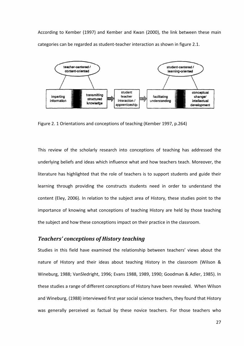
27

According to Kember (1997) and Kember and Kwan (2000), the link between these main

categories can be regarded as student-teacher interaction as shown in figure 2.1.

Figure 2. 1 Orientations and conceptions of teaching (Kember 1997, p.264)

This review of the scholarly research into conceptions of teaching has addressed the

underlying beliefs and ideas which influence what and how teachers teach. Moreover, the

literature has highlighted that the role of teachers is to support students and guide their

learning through providing the constructs students need in order to understand the

content (Eley, 2006). In relation to the subject area of History, these studies point to the

importance of knowing what conceptions of teaching History are held by those teaching

the subject and how these conceptions impact on their practice in the classroom.

Teachers’ conceptions of History teaching

Studies in this field have examined the relationship between teachers’ views about the

nature of History and their ideas about teaching History in the classroom (Wilson &

Wineburg, 1988; VanSledright, 1996; Evans 1988, 1989, 1990; Goodman & Adler, 1985). In

these studies a range of different conceptions of History have been revealed. When Wilson

and Wineburg, (1988) interviewed first year social science teachers, they found that History

was generally perceived as factual by these novice teachers. For those teachers who

28

majored in Social History, History was seen as interpretation, as well as fact, and the study

of History was seen to be full of life, including music, art and drama. However, among non-

History majors, teaching History was more often viewed as arcane, dusty and dull (Wilson,

2001). According to Wilson and Wineburg (1988), the different knowledge and beliefs of

teachers influence what they do in the classroom; ‘those who saw History as interpretative

and exciting, craft instruction to communicate those aspects of discipline. And those who

saw History as “the fact” or who had little historical knowledge had fallen into the age-old

routine of uninspired History teaching’ (Wilson, 2001, p.535).

In another study, which explored the relationship between teachers’ conceptions of History

and their teaching style, five conceptions of teaching History were found (Evans, 1990). The

data were drawn from 30 teachers, with five teachers being interviewed and observed in-

depth. He also interviewed the students of these five teachers.

Evans (1990) categorized these teachers into five types according to their conceptions of

teaching History. These were:

Storyteller, where teachers’ talk dominated the classroom and storytelling (or

narrative) was used as the common mode of communication.

Scientific historian, who focused on historical explanation and interpretation,

understanding historical processes and gaining background knowledge to

understanding current issues, while encouraging students to engage in inquiry.

Relativist /reformer, who emphasised the relationship of past problems to present

ones.

29

Cosmic philosopher, who saw generalisations as the most interesting aspect of

History.

Eclectic teacher who selected different emphases at different times.

These widely varying conceptions of teaching History were not regarded as exclusive

categories. Rather each category emphasised different purpose for the study of History.

Evans (1990) concluded that teachers’ conceptions of History seemed to be related to their

background, beliefs, and knowledge. But, he cautioned that other factors such as

organisational constraints and models of teaching could have an impact on teaching styles

and teachers’ conceptions of History.

Wineburg and Wilson (1991) undertook in-depth interviews and observations with 11

experienced high school History teachers, with the purpose of capturing, and describing

what these teachers knew, thought and did. Comparing the case of two teachers, Price and

Jensen, as examples, they claimed that both of these teachers presented subject matter in

two ways, namely, by focussing on epistemological issues (the way of knowing History) and,

on the other hand, on contextual issues (specific concepts, ideas and events). Both

teachers presented subject matter in a way that helped students to see the complexity of

historical understanding. Although their teaching differed, both of them had considerable

subject knowledge. Their teaching was shaped by their views of History as well as by their

knowledge and understanding of what students knew and cared about, what curricular

resources were available and what parents expected of the school. This study highlighted

the way an individual teacher’s knowledge and beliefs were able to shape teaching in the

classroom.

30

As a result, it is essential to better understand how teachers’ conceptions of History

teaching can influence students’ approaches to learning History. The next section considers

what makes History teaching effective in the classroom.

Characteristis of Effective History Teaching

The literature suggests that effective History teaching involves the teacher and students

focusing on knowing History (subject-matter), ‘doing’ History (historical inquiry), and

‘scaffolding’ the learning of History through their pedagogical knowledge and skills. To ‘do’

History involves analysing evidence in order to represent past events, considering

perspectives and context, going beyond the written words to understand the intentions,

motives, plans and purposes of an author so as to build understanding of the historical

significance of the events concerned (Hover & Yeager, 2003). Scaffolding refer to the

teaching supports that facilitate learning when students are first introduced to new

subjects or concepts (McKenzie, 1999; Bransford, 2000; and Baneszynski 2000).

One of the characteristics in effective History teaching is the teachers’ recognition of

History as a unique subject. History is about inquiring into and representing human

experience of the past. Teachers need to have a good knowledge of the subject matter to

enable them to analyse curriculum material and to transform it into suitable teaching

material (National Education Blueprint, 2007; Garner & Mansilla; 1994, Yilmaz; 2008).

Moreover, Yilmaz (2008) suggested that the History teacher also needed to have a strong

understanding of the conceptual foundation of the discipline. Teachers should have

historical knowledge and skills in order to encourage and help the students in the History

classroom to understand the past.

31

Historical inquiry engages students in actually doing History. Levstik (1996) and Levstik and

Barton (2001), suggests it involves students in posing questions, collecting and analysing

sources,so that by the end of the process, students build their own historical

interpretations. In doing History with a group of students, an effective teacher presents

History as a constructive activity that historians do, working with raw materials, in order to

tell the past, and understand the present.

Content knowledge is essential for History teachers (Shulman, 1987). This view is

supported by VanSledright (1997) who suggested that applying subject knowledge in the

classroom meant approaching History effectively from the inside out. In doing this,

teachers would structure lessons in the classroom, by asking historical questions, while

students would adopt historical inquiry skills, such as investigating, scouring, reading, and

analysing evidence. As they answered the questions given by their teachers, they would

develop their own interpretation of events. To be able to ‘do’ History with their students in

this way, teachers must understand the content knowledge involved in History

methodology.

Teachers with greater subject content knowledge are also able to involve students in

discussion that goes beyond text book content, to ask higher-level cognitive questions, and

to guide students to work on their own directed activities (Carlsen 1987; Carlsen & Wilson,

1988; Dobey & Schafer, 1984; Hasweh 1985 cited in Covino & Iwanicki, 1996). Clearly,

content knowledge is a major factor in effective History teaching in schools. Teachers who

know the content knowledge are able to deliver the subject more effectively. In addition,

to knowing the content knowledge, understanding historical inquiry is of major importance

for teachers. Embedding inquiry into History teaching involves students analysing evidence

32

from various sources (e.g. archives, texts) in order to construct a representation of past

events, thereby going beyond the written word and building understandings of historical

significance (Hover & Yeager, 2003).

Pedagogical content knowledge is another factor that influences teachers’ competence in

helping their students to learn History. According to Shulman (1986, p. 9), pedagogical

content knowledge ‘goes beyond knowledge of the subject matter per se to the dimension

of subject matter knowledge for teaching’. Teachers need knowledge of the various

strategies to extend the understanding of students in the classroom and overcome

misconceptions (Shulman, 1986). This view is supported by Seixas (1999, p.313), who

suggests that subject matter by itself is inert knowledge, while pedagogy is concerned with

the means of its ‘delivery’. Furthermore, Yilmaz (2008, p.43) suggests that:

The more knowledgeable a History teacher is about pedagogical

content knowledge, the more likely it is that he or she is going to

adjust curriculum and instruction to students’ abilities, learning

styles, pedagogical preferences, needs, interests, and cultural

background.

A teacher’s great responsibility is to help students to structure learning; this is built up

slowly in the process called scaffolding discussed earlier (Levstik, 2000). Effective History

teachers are able to scaffold learning in the classroom by constructing a context for

historical inquiry which helps to motivate learning. Such teachers are also able to connect

current knowledge with new knowledge while teaching in the classroom. As an educator, a

teacher should develop students’ understanding of historical evidence and interpretation,

and through scaffolding, encourage deep knowledge of History. Having strong pedagogical

33

content knowledge skills seems to be a prerequisite for History teachers (Keith, 2004), but

it needs to be complemented by classroom strategies for teaching.

Methods in Classroom Teaching

In general, teachers have built up their conceptions about teaching (discussed in an earlier

subsection) from personal experiences in their own elementary to university level

education (Peeraer, 2011; Dall’Alba, 1990; Fox, 1983; Martin & Balla, 1991; Pratt, 1992;

Prosser, Trigwell & Taylor 1994; Ramsden, 1992; Samuelowic & Bain 1992). In the

classroom they teach their own students using a variety of practical methods and activities,

which are consistent with their conceptions of teaching, to deliver the subject content

knowledge.

Recently, Trigwell (2012), investigated the relationship between teachers’ emotions and

their method of classroom teaching in various courses in higher education. The 175

participants were all teachers in the Australian higher education sector. Two self-report

questionnaires were used: (a) Approaches to Teaching Inventory (ATI-R), and (b) The

Emotions Teaching Inventory (ETI). These questionnaires were used to obtain the

information on the following themes: different approaches to teaching (conceptual change

or student focused (CCSF) and information transmission or teacher focused (ITTF); teachers’

emotional experiences (positive emotions: motivation, pride, confidence, satisfaction and

happiness; negative emotions: anxiety, embarrassment, frustration, boredom and

annoyance). The researcher found that there were relationships between the approaches

to teaching their courses and their emotions about teaching it. Teachers did experience

both positive emotions (motivation and pride) and negative (anxiety and embarrassment)

in their teaching. The positive emotions were associated with those respondents who had

34

CCSF approach to teaching. On the other hand, the negative emotions were associated

with teachers having the ITTF (Trigwell, 2012).

A another study carried out by Zerihun, et al. (2011), in the Department of Psychology at

University of Mekelle, Ethiopia, focussed on teachers’ approaches to teaching and students’

learning, and teacher conceptions of the meaning of teaching. The data were collected

through survey questionnaires. Two questionnaires were designed, one for teachers and

one for students. A total of 434 respondents from students and 43 respondents from

teachers were used for the analyses. The results indicated firstly that teaching was seen as

predominantly teacher-centred. Both teaching and learning activities evolving from this

orientation. This meant that, the teacher was transmitting knowledge rather than

facilitating student learning. Secondly the teacher was regarded as the provider of

information. Both set of participants indentified effective teachers as those who showed

the following characteristics: knowledgeable, punctual, organised and good at

communicating (Zerihun, 2011).

Kember and Leung (2005) conducted a large scale study on 2,548 full-time and part time

students in a Hong Kong university to examine the relationship between teaching

approaches, student teacher relationships and student outcomes (learning, working

together, and intellectual outcomes) (see the path diagram in Kember & Leung, 2005, p.

165). The researchers found a significant relationship between the teaching approaches

and other variables. The results indicated that there was a mutually reinforcing effect from

good teacher-student relationships (Kember & Leung, 2005, p. 115). Moreover, the effect

of teaching approaches on students markedly outweighed the weaker influence of the

wider university environment. Finally, the study revealed that students with different

35

modes of enrolment (full-time as compared to part-time) experienced different types of

teaching approaches (Kember & Leung, 2005, p. 166).

Lindblom-Ylanne, Trigwell, Nevgi, and Ashwin (2006), in a study carried out on teachers

from the University of Helsinki, investigated the relationships between their approaches to

teaching, their self-efficacy belief, as well as the effect of teaching contexts, on approaches

to learning. The research stated that ‘there is evidence that teachers’ approaches to

teaching are connected with their conception of teaching’ (Lindblom-Ylanne et al., p. 286).

Findings showed that teachers who experienced different contexts adopted different ways

of teaching. Teachers from different disciplines also used different approaches to teaching.

In particular, teachers from the ‘hard discipline’ areas (physical sciences, engineering, and

medicine) adopted teacher focussed approaches. In contrast, teachers in the ‘soft

discipline’ areas (social sciences and humanities) were more student-focused (Luedddeke,

2003 cited in Lindblom-Ylanne, et al., 2006). There was no significant difference in self-

efficacy belief of teachers across the disciplines. The researchers concluded that

encouraging teachers to adopt more student-centred approaches could be triggered by a

focus on courses regarded as less mainstream (Lindblom-Ylanne, et al., p. 295).

Trigwell. et al., (1999), examined a group of 46 science teachers and their students (3956)

to determine the relationship between teachers’ approaches to teaching and students’

approaches to learning. Furthermore, this study also included links between these factors

and student learning outcomes. The results revealed that teachers who employed an

information or teacher-focused approach to classroom activities were likely to be teaching

students who reported adopting a surface approach to learning in the classroom. This

36

result also affirmed that surface approaches to learning were related to lower quality

learning outcomes, as the previous research had revealed (Trigwell, et al., 1999, p. 66).

A number of other studies have shown no relationship between approaches to teaching

and students’ learning. Selcuk (2010), for example, investigated the effects of the Problem

Based Learning (PBL) method on pre-service teachers’ achievement, and learning

approaches and attitudes towards, physics. The respondents were 46 pre-service students

teacher in Turkey. The findings suggested that the adoption of the PBL teaching approach

had encouraged student learning and improved student interest in physics.

A similar study was carried out by Kek and Huijser (2011) on the combined relationships of

student and teacher factors on learning approaches and self-directed learning readiness.

The samples were 392 students and 32 teachers from one of the public universities in

Malaysia. A Problem Based Learning (PBL) approach was employed in 44 classrooms. The

researchers revealed how and what individual student factors and teacher factors

influenced students’ learning approaches and related learning outcomes (Kek & Huijser,

2011, p. 190).

Another study, carried out in the Netherlands by Torenbeek,Jansen, and Hofman (2011, pp.

364-365). They investigated the approaches to teaching at secondary schools, their

relation to students’ perception of the fit between school and university, and their first

year university achievement. The data were collected using a questionnaire for teachers

and students and an interview for school management. The results indicated that the

approaches to teaching at secondary school impacted on first-year university results and

the perceived fit for students enrolled in soft sciences. Students who experienced teacher-

centred teaching in secondary school performed well in university compared to students

37

who were exposed to student-centred learning. The long-term effect of a certain approach

to teaching in secondary schools might be different from any short term effects evident in

students’ development. The effect of student background characteristics was found to be

important, in addition to the effect of teaching approaches.

Another recent study investigated (a) what teachers of undergraduate medical programme

in University of Antwerp, Belgium thought about their own learning; (b) how they

approached their teaching; and (c) the relationship between their conceptions of learning

and their teaching approaches (Peeraer, Donche, De Winter, Muijtjens, Remmen, Van

Petegem, Bossaert , and Scherpbier 2011, p. 33). It was found that teachers in this

programme had a variety of conceptions of their own learning (COL), but no significant

correlations were found between COL and their approaches to teaching (Peeraer, et al.,

2011, p. 32).

The following section discusses other studies that focussed on students’ approaches to

learning.

2.4 Students’ approaches to learning

Students’ approaches to learning were originally conceptualised by Marton (1975, cited in

Biggs & Moore, 1993) in the context of student literacy. He found two types of learning

approaches: surface and deep learning. A surface approach was related to lack of interest

of subject matter, so that students with this approach tended to memorise facts.

Meanwhile, the deep learning approach was when students sought to understand the

underlying meaning of the learning task.

38

Biggs (1987) extended Marton’s work by focusing on different aspects (Biggs & Moore,

1993). Biggs proposed that the students’ learning approaches were a mixture of motives

and associated strategies. He identified three types of motives as follows: deep, surface,

and achieving (Biggs, 1987). A student who used a surface approach to learning tended to

memorise or rote learn, in order to reproduce the material given, while in the deep

approach to learning, students attempted to seek meaning for themselves and to

understand the materials. According to Dart (1997), a deep learning approach was

associated with a constructivist teaching stance, which emphasised that learners actively

construct knowledge. On the other hand, the surface approach to learning was connected

to learners’ passive reception of teaching (Dart, 1997). In the achieving approach to

learning, students were motivated by achieving high grades, and responded by organising

their time to get the best results. This approach included a mixture of deep and surface

approaches to learning, but only for the purpose of maximising assessment results.

Biggs (1987) developed the Learning Process Questionnaire (LPQ) and the Study Process

Questionnaire (SPQ) to assess how students at secondary school and tertiary level

approached their learning tasks in general. The questionnaire was based on his motivation

and strategies model.

Entwistle and Ramsden’s (1983) subsequent research on students’ approaches to learning

found a fourth type of students, the non-academic, who really represented failure to learn.

Ramsden (1992) claimed that the deep approach involved reading for understanding,

active processing of information and making connections between previous knowledge and

current information. In contrast, surface learners used rote learning simply to retain the

information. Meanwhile, in the achieving approach to learning, students focused on a

39

studying strategy that would maximise results. In case of students with a non-academic

approach to learning, they lacked motivation, were negative in attitude, and disorganised

(Entwistle & Tait, 1990). Other studies, however, found that students’ approach to learning

was not fixed, but flexible (Booth, 2003). Students could change their approach depending

on the context. The main influence on student approaches in the educational environment

was established by the instruction provided by teachers in the classroom (Booth, 2003).

A series of studies by Biggs’ (1978, 1985, 1987) confirmed that the personal characteristics

of students and their learning context were the essence of Biggs’ conceptualization of

students’ learning approaches. In developing and validating the Study Process

Questionnaire (SPQ), Biggs (1985 & 1987), used a huge sample of students’ data and range

of contextual and personal characteristics as independent variables. The variables used in

SPQ were gender, age, year of study, parents’ education background and academic stream

(Arts/ Science). The results indicated that females scored lower than males on the surface

learning approach and higher on the deep learning approaches. In terms of age, younger

students were more likely to adopt a surface approach compared to the older students.

Years of study had a strong positive effect toward deep and achieving learning approaches.

In addition, the results showed that students from the Arts and Education disciplines were

high on the deep learning approach, in contrast to Science students who were low on the

deep learning approach.

A number of other researchers found that there were relationships between deep

approaches to learning and student perceptions of the teaching context (Kember & Gow,

1994; Dart, 1994; Kember & Wong, 2000; Leung & Kember, 2003). Their results highlighted

some factor in teachers’ qualities that were associated with students’ deep approach to

40

learning. These qualities were identified as being a motivator; encouraging interactive

learning; providing pastoral care; and using a variety of teaching methods. Leung and

Kember (2003) claimed that if students were given the opportunity to reflect, to explore

and to think about their work, it would encourage the deep approach to learning in the

classroom.

Similar findings were obtained by Lizzio, Wilson, and Simon (2002) in a study investigating

the relationship between students’ approaches to learning and their classroom

environment. The researchers found that the classroom environment was not the only

influence on students’ learning approaches. The findings from Lizzio and associates

revealed that a heavy workload and inappropriate assessment would lead the students to

employ a surface approach to learning. In contrast, that students were encouraged to use

deep approaches where they perceived the learning environment to be interesting and

motivating, and were given appropriate workloads and assignments. These researchers

provided five important suggestions for a quality teaching in the classroom. First, ‘the staff

show an interest in students’ opinions and attempt to understand the difficulties students

may be having; second, express positive expectations and seek to motivate students to do

their ‘best work’; third, provide clear and useful explanation of ideas; fourth, work to make

subjects interesting and finally provide feedback on progress’ (Lizzio et al., 2002, p. 50).

Another study, carried out by Furnham, Christopher, Garwood, and Martin (2007) focussed

on personality factors, general knowledge and approaches to learning. Three types of

questionnaires were used in this study. The first was Irwing’s General Knowledge Test

(Furnham, et al., (2007), with 72 items that measured knowledge of six areas: literature,

general science, medicine, games, fashion, and finance. The second was The NEO

41

Personality Inventory - Revised (NEO-FFI; Costa & McCrae, 1985, 1992, cited in Furnham,

(2007), that measured the ‘Big Five’ personality factors: neuroticism, extraversion,

openness to experience, agreeableness, and conscientiousness. The third questionnaire

was The Study Process Questionnaire (SPQ) (Biggs, 1987), which investigated three learning

approaches: Deep, Surface and Achieving, which were broken down to two components:

learning motives and learning strategies. In total there were six factors for analysis: deep

motive, deep strategy, achieving motive, achieving strategy, surface motive, and surface

strategy. The results found that older males scored higher, compared to females, on the

general knowledge score. Moreover, both age and gender were significant predictors of

general knowledge, that is, as people got older they increased their general knowledge,

due to activities such as reading and remembering more. In terms of personality, the

results revealed that there was no significant difference between five sub-scales that were

tested as predictor variables of learning approaches. The researchers did found that the

relationship between openness and achievement in general knowledge was mediated by a

deep approach to learning.

According to Baeten, (2010), student characteristics such as age, personality, methods,

motivation, self- confidence and self-efficacy all impacted on students’ learning, as well as

teaching. Furnham et al., (2007) affirmed that age and personality are both factors which

are not able to be manipulated. As students grow older and their personalities are

moulded by ‘Big Five’ factors (neuroticism, extraversion, openness to experience,

agreeableness, and conscientiousness) they seem more likely to adopt deep learning

approaches.

42

From the above discussion of research studies, it is clear that demographic personal

variables such as age and gender, as well as teacher and student characteristics, are related

to students’ approaches to learning. These influence students’ motivation to learn for

understanding and engage in learning in the classroom. Another important factor feeding

into this is students’ perceptions of the classroom learning environment.

Students’ perceptions of classroom learning environment

Studies on classroom climate or learning environment have been carried out to investigate

its effect on students’ learning at secondary and university level (Fraser, 1991) and its

influence on their learning approaches (Ramsden, Martin, and Bowden, 1989; Dart,

Burneet, Purdie, Boulton-Lewis, Campbell, and Smith 2000).

Students’ perceptions of their preferred and actual learning environments in their

classroom varied. Yuen-Yee and Watkins (1994) found that students in one Hong Kong

secondary school preferred their classroom environment to be safe and supportive,

encouraging active participation in the learning process, and incorporating investigation

skills in learning science in the classroom. Previous research results had showed that such

an environment promoted a deep approach in student learning. However, students also

perceived that in fact, their classroom was relatively competitive, teacher controlled and

encouraging of rote-learning. It was shown in this study that students preferred a friendly

classroom learning environment where teachers and students could work together to

develop better activities in the classroom. A classroom perceived to be high in such

personalisation was likely to promote deep learning.

MacAulay (1990), discussed four domains, (a) structure and organization, (b) cognitive

process, (c) student characteristics, and (d) teacher characteristics, in her review of the

43

classroom environment. MacAulay’s (1990) study was based on the Moos (1980)

framework. The influence of each domain was examined separately and discussed. The

findings indicated that structure and organization - the physical features in the classroom -

could influence students’ outcomes. Cognitive process - the self-management techniques

designed to encourage a democratic classroom environment - when tested in the

classroom, promoted students’ schooling achievement.

Student characteristics - the students’ preference for a co-operative climate compared to a

competitive climate. Furthermore, the students were more motivated in learning and

achievement in the former. Teacher characteristic - teachers who were friendly, supportive,

warm, and communicative - were preferred by the students, who considered that such

teachers increased their learning outcomes and enhanced the emotional climate in the

classroom. The results of this study indicated the importance of the teacher’s role in

motivating and improving the learning experiences of the student. In the students’ point of

view effective teaching depended on the personality of the teachers.

Fraser (1998) used five dimensions, namely personalisation, participation, independence,

investigation and differentiation, to examine the nature of the classroom learning

environment in the classroom and its influence on students’ characteristics and students’

experiences. His findings showed that students’ perceptions of the classroom environment

influenced their approaches to learning and the quality of their learning outcomes (Fraser,

1989; 1998).

A similar view was put forward by Dart et al. (1999) who concluded that students who

perceived the classroom environment as cohesive, having order and organisation, and

encouraging participation, and clear goals were likely to show higher levels of achievement.

44

Dart’s study of the relationships between students’ perceptions of the classroom

environment, approaches to learning and self-concept as a learner, was carried out in

Australia, using the Individualised Classroom Environment Questionnaire (ICEQ) and the

Learner Self Concept Scale. The results indicated that there was a significant relationship

between the deep approach to learning and a classroom environment, which students

perceived to be highly personalised, encouraging active participation in the learning

process and developing investigation skills in learning. On the other hand, the surface

approach to learning had negative associations with classroom environment and learning

approaches, because students who employed surface approach to learning indicated lower

levels of personalisation, participation, and investigation in the classroom learning.

In subsequent research, Dart et al. (2000) tested the relationships between student

conceptions of learning, their perception of the classroom environment and their

approaches to learning, using structural equation modelling. They found important

relationships between the variables. The findings showed that the deep approach to

learning was promoted by the teachers, when the students perceived that the classroom

environment was safe and supportive. Furthermore, in this environment, teachers could

use several methods (exploration, inquiry and experiments) for problem solving. This

research also found that deep learning could be facilitated by the daily experience of such

activities. However, Dart and associates added that student skills and willingness to learn

were essential, as well, to improve learning. It can be concluded that learning strategies

which nurture deep learning in the classroom, are required in building up a positive

classroom environment.

45

Evans, Harvey, Buckley, and Yan (2009) also perceived classroom climate as a multi-faceted

concept which comprised various dimensions. According to Evans et al. (2009) there were

three different components in classroom climate (a) academic, (b) management and (c)

emotional. Their research focused on emotional climate, for which they identified five

components: (a) emotional relationship, (b) emotional awareness, (c) emotional coaching,

(d) emotional intrapersonal belief, and (e) emotional interpersonal guidelines. Evans et al.

(2009) suggested that it was essential to treat emotional climate as a separate aspect of

the classroom climate because it was superior to other classroom climate domains in

interfacing with the academic and management elements in an effective learning

environment. In this sense, they claimed that emotional climate could be regarded as an

aspect of all teacher-child interaction, rather than a separate component of the classroom

environment. The results also indicated that there were relationships between classroom

climate and students’ cognitive, social, and motivational development. Furthermore,

Jennning and Greenberg (2009) (in Evans et al., 2009) considered that the emotional

climate depended on teacher’s competence emotionally and socially, when dealing with

complex interactions involving all students in the classroom. Therefore, Evans and his

associates suggested that the most important factors in the classroom environment were

the teachers’ instructional style and classroom management. He added these factors were

a function of the emotional relationship between teacher and students.

There are very few studies on the students’ perspective of the classroom environment in

History teaching. According to Ylijoki (1994), intrinsic interest in choosing History as a

course in the university was one of the factors that influenced students’ positive

approaches to learning. The implication is that students should have an interest in subjects

46

they choose because it can affect their performances (Booth, 2003). However, the situation

is different in the Malaysian secondary school context since History is a compulsory subject.

Students’ interest in History, however, can be sustained if teachers play their role

effectively. In particular, the way which in History is taught is important for sustaining a

deep approach to learning. Both students and teachers in History have the responsibility to

form a suitable classroom environment in order to expand the deep approach to learning

among the students. Students have responsibility to do the preparation, and the teacher’s

task is to facilitate the discussion (Booth, 2003). The variety of methods that a teacher can

use is another possible factor that affects the students’ perception of learning History in

the classroom. Using primary sources, novels, maps, cartoons, films, videos etc can make a

History lesson come alive. In addition, using different teaching pedagogies also could

accommodate variation in students’ learning styles (Booth, 2003). This view is supported by

Hayden, Arthur, And Hunt (1997, p.201) who suggested that ‘resources certainly help

students to be active in learning and can often play a significant part in motivating them to

do well in History’.

Overall, the research studies reviewed were more on the university setting rather than the

school, with focus on the science subjects more than History. Furthermore, the review

revealed that little classroom research related to classroom environment has been

published in the Malaysian context. However, the findings from the range of literature

reviewed confirm the key variables which influence the way teachers teach and students

learn in the classroom. The following section discusses the Biggs’s 3P Learning Model as the

theoretical framework used to guide this present study, as well as various Research

Modelling Approaches that can be used for data analysis.

47

2.5 Theoretical Framework

Biggs’ 3P Model of Student Learning

The initial purpose of this research was to investigate the differences between out-of-field

and in-field teachers in relation to students’ learning of History in the classroom. The

models reflect the relationships between the variables discussed in this study. This study

was guided by the Biggs’ 3P (Presage, Process, and Product) theoretical framework for

understanding students’ learning through the relationships between what teachers and

students think and do, and the nature of students’ outcomes. The relationships in the

Biggs’s 3P model among these variables are shown in Figure 1.

The Biggs’ 3P Model has been adopted as the theoretical framework for this research

because it shows clearly how students’ learning outcomes are influenced by students’ own

personal characteristics, interacting with teacher characteristics and the teaching context

through the learning activities of the classroom. Put another way, Biggs’ 3P Model of

Student Learning, describes three points in time as they relate to learning: presage

(personal and situational factors), process (activities in the classroom) and product

(student learning outcomes) as represented in Figure 2.2 (Biggs 2003).

This theoretical framework is particularly appropriate for a study that seeks to examine the

relationship between the characteristics and qualifications of History teachers and their

students learning outcomes in History in Malaysian secondary schools. In the discussion of

the three time points that follows, the variables under each factor have been

conceptualised in terms of the present study.

48

PRESAGE PROCESS PRODUCT

Figure 2. 2 Adapted from Biggs (2003).Theoretical Framework based on Biggs’ 3P Model of Student Learning

Presage factors are the pre-existing factors that influence students’ learning outcomes.

Generally there are two categories of presage factors: students characteristics and teacher

factors. In the context of this research, the first category has been conceptualized to

include students' characteristics, and perceptions of classroom environment. The second

category includes teacher characteristics, teacher qualifications, and conceptions of

teaching in general, as well as the more specific factors of teachers’ conceptions of History

teaching, and Teaching Methods.

Process factors are the result of interactions between the presage factors of students and

teachers in classroom learning activities. This interaction influences the students’

immediate and ongoing approach to a particular task. Whether students manage the

LEARNING OUTCOMES

- Perceptions of History and how It is taught - History learning objectives

TEACHERS & TEACHING-CONTEXT

- Teacher Characteristics - Teacher Qualifications - Conceptions of teaching - Teaching Methods

History curriculum

Curriculum

Classroom Climate

STUDENT

- Student characteristics - Perceptions of Classroom Climate

LEARNING-FOCUSED ACTIVITIES

- Learning & Teaching Approaches (Deep/Surface/Achieving)

49

learning task with deep, surface or achieving approaches depends on their perception of

teachers’ presage factors, such as teaching characteristics and teacher practices, and

teaching conceptions. A learning approach is considered deep when students seek in-

depth meaning and understanding of the material being studied. In this approach students

are actively constructing knowledge for themselves. This is because, according to Biggs and

Moore (1993), Dart (1997), and Tang (1998) the deep approach is associated with

constructivist learning. In contrast, the surface approach to learning is related to rote

learning, which is in line with the traditional transmission model of teaching. In this

approach students receive knowledge from the teachers and respond passively (Biggs &

Moore, 1993; Dart, 1997; Tang, 1998). In the case of the achieving approach to learning,

students become focussed on a studying strategy that maximises results for the purpose of

ego enhancement, excelling in organized activities and cue-seeking behaviours (Dart et al.,

2000).

Product factors refer to the outcomes achieved of student learning. According to Biggs and

Moore (1993), the quality of outcomes is partly influenced by the learning approaches

adopted by the students. Poor quality outcomes are mainly associated with surface

learning approaches, while high quality outcomes are associated with deep learning

approaches. It is important to recognise that for this investigation learning outcomes are

gauged or measured not by objective marks related to students’ achievement level in tests

on examinations. Rather, in this study the learning outcomes refer to students’ perceptions

of History and how it was taught, as well as how far History learning objectives were being

achieved in the classroom.

50

Biggs’ 3P Model of students’ learning outcomes has a dual base of presage factors,

recognising the importance of inputs from both students and teachers. In this study the

Process stage operates between teachers and students as they interact in the learning of

History in Malaysian classrooms. It was expected that the results would highlight the

influence of students’ different personal and situational backgrounds on the final learning

outcomes. Understanding these factors is important for teachers striving to improve their

own pedagogical practices.

Nevertheless, the main focus of this study was to test a model to investigate how teacher

factors affect students’ learning outcomes. In particular, the study sought a better

understanding of how effectively teachers function in the history classroom, especially out-

of-field as compared to in-field teachers. The judgement on this issue came from the

students’ perspective. Their perceptions on the subject, History, and the quality of their

learning in the History classroom were used to measure students’ learning outcomes.

Keeves’s Modelling Approach Applied to Research Data

Keeves (2002) recommended that it is essential to adopt a Modelling Approach to the

accumulation of knowledge both in regard to personal learning and to research

investigations. Moreover, once developed, models must be tested and evaluated for their

‘coherence and adequacy’ (Keeves, 2002, p. 114).

Keeves considered that both individual and corporate knowledge must be tested not only

for coherence, but also against evidence obtained from the real world in which human

beings are living and undertaking their inquiries (Keeves, 2002, p 115). To do this, it is

essential to develop a model for testing, beginning with the expression of the key

51

relationships in propositions or hypotheses. The hypotheses then require structuring into a

model which can be formulated for testing.

There were five types of models recognized by Keeves (1997, pp 388-390): (a) analogue

models, (b) semantic models, (c) schematic models, (d) mathematic models, and (e) causal

models. However, these models could have limitations, as Keeves (1997, p.121) pointed

out, through ‘oversimplification and inappropriate signification in which significance is

attached to inappropriate aspects of a model rather than reveal the structural aspect of

importance’.

Causal Model

The Causal model has been employed to guide this study. The causal model was introduced

in the field of educational research in the early 1970s. Originally, this model was used in

the field of genetics and linked with the analytical techniques of path analysis. Through the

work of Burks (1928), Parker (1971) and Blalock (1961) (cited in Keeves, 1997), the causal

model was made available for use in the educational field. In general, the model is the

combination of the principles of path analysis and a set of structural equations. The idea

underlying this model is constructing a ‘simplified structural equation model of the causal

process operating between the variables under consideration’ (Keeves, 1997, p 391).

Keeves added that, in the modelling approach, logic and statistics are used to test the

sufficiency of the model. Besides these, testing of the model can also be carried out using

controlled observation, experimentations or systematic collecting of evidence from the real

world (Keeves, 1997, p 121). Finally, the model can be evaluated either as acceptable or

unacceptable from the results of the test. In this study, Biggs’ 3P conceptual framework for

52

learning outcome in education has been developed into a causal model, and tested using

Structural Equation Modeling (SEM) and Partial Least Square Path (PLSPATH).

In this study the causal model was used to guide the collecting and analysing of the

quantitative data. The conceptualizations of relationships were derived from the literature

and empirical evidence from previous studies. How this model shaped the current study is

explained below. There are a number of presage, process, and product factors in this study:

(a) teachers’ and students’ characteristics, (b) learning process, and (c) learning outcomes.

The relationship between the factors can be illustrated as follows (a) (b) (c). The

causal model used in this study is in line with its purpose which is to measure the direct

and indirect influence of each variable that is involved in this study and also to investigate

the variability of effects from each particular cause. Furthermore, the teachers’ and

students’ characteristics have the potential to be treated as one or more causes of

particular affects in the teaching and learning of History in the classroom. All variables used

in this study can be tested statistically using statistical procedures such as Path analyses

and structural equations modelling (SEM) to check the significance and magnitude of the

relationships between the causal and effects. This procedure is discussed in detail in

Chapters 7 and 8.

2.6 Summary

The discussion of previous research studies related to this topic began with a specific and

quite narrow focus - the nature of out-of-field teaching and its impact on the classroom

teaching of History in Malaysia. Out-of field teaching was defined as teachers who do not

have a university degree in History or teachers who do not hold a tertiary major or minor

qualification in History education (Ministry of Education, 1991 cited in Aini Hassan et al.,

53

2007). It most often occurs as the result of mis-assigned teachers (Harris and Jensz, 2006)

or insufficient supply and training (Ingersoll, 2002). While previous studies indicated that

teacher qualifications had a significant relationship with student achievements, (OECD

2005, 2009, Goldhaber & Brewer, 2000), none had actually investigated out-of-field

teachers at the school level and the relationship of their teaching to students’ learning of

History in the classroom. A review of studies influencing classroom teaching and learning

highlighted the importance of conceptions of teaching and their influence on students’

approaches to learning, factors in effective History teachings and students’ perceptions of

classroom climate.

The last section of the chapter described Biggs’ 3P Model of student learning as the chosen

framework of variables for this study and out-lined how it was adapted to this research

topic. In addition, the importance of the Modelling Approach to data collection and

analysis was explained. The choice of the Causal Model, which used Structural Equation

Modeling (SEM) and Partial Least Square Path (PLSPATH) analysis to test the relationship

between variables was justified. The results of this research were expected to enhance

understanding of how the teacher factors identified interact with student factors to

influence student perceptions of teaching and learning in the classrooms of in-field as

compared to out-of-field teachers. The next chapter discusses the methodology of the

research in detail.

54

Chapter 3 Methodology __________________________________________________________________________

3.1 Introduction

In this chapter, the setting up of the research is explained in relation to the method and the

questionnaires used. There is an outline of the approval process in Adelaide and Malaysia,

together with a description of the pilot study carried out. A detailed discussion follows

concerning the sampling process in the selection of the respondents and the procedures

used for data collection. Finally, the chapter discusses the statistical analysis techniques

employed to confirm the validity of the instruments by testing the fit of the various models

related to the theoretical framework, proposed at the end of Chapter 2. In addition, the

Partial Least Square (PLS) and Hierarchical Linear Modelling (HLM) statistical techniques

used for testing the relationships between the factors in the study are explained.

3.2 Method used in this study

This research adopted a quantitative research survey method. The data were gathered by

using survey questionnaires. Statistical analyses were employed to investigate the trends of

the responses given and to test the research questions (Cresswell, 2008). In addition,

correlational research design was employed. According to Creswell (2008), this design

enables the researcher to test and describe the degree of relationship between two or

more variables or sets of score. In this study, quantitative methods were used to

investigate relationships between teachers’ conceptions, methods and teaching

approaches and students’ approaches to learning History, their classroom learning climate,

and History learning outcomes.

55

3.3 The Questionnaires

This section describes the instruments that were used in this study. There were two sets of

questionnaires used, one for the teachers (refer to Appendix 1) and another for students

(refer to Appendix 2). Each set of the questionnaires had three parts as follow:

Teachers’ questionnaire:

Teachers Conception of Teaching by Gao & Watkins (2002).

Approaches to Teaching Instruments (ATI) by Trigwell, Prosser & Ginns (2005)

History Teaching Method (self- developed)

Students’ Questionnaire:

Individualised Classroom Environment Questionnaire (ICEQ) by Fraser (1990)

Biggs’s Learning Process Questionnaire (LPQ) by Biggs (1987)

Students’ Perception of History (self- developed)

The first two parts in each set were standardised and validated instruments that have often

been used in educational contexts but needed Confirmatory Factor Analysis (CFA). The

third parts in each set was developed by the researcher specifically for this study. It

therefore required validation through Exploratory Factor Analysis (EFA) and CFA.

Each of the above questionnaires is discussed in subsequent sections, with those for

teachers being considered first.

Teachers’ Conceptions of Teaching

The School Physics Teachers’ Conceptions of Teaching (SPTCT) instrument was adapted to

investigate History teachers’ conceptions of teaching in this study. Gao and Walkins (2002)

developed this instrument to assess teachers’ conceptions of teaching among a large

56

sample of Physics teachers in order to discover the relations between teachers’

conceptions and student learning.

This instrument consisted of 37 items. Each item expressed teachers’ opinions or ideas

about teaching and learning. SPTCT measured five scales, namely, knowledge delivery (KD),

exam preparation (EP), ability development (AD), attitude promotion (AP) and conduct

guidance (CG). These scales were described by Goa and Watkins (2002) as follows:

1. Knowledge delivery (KD) is based on the conception that learning is a process of

acquiring or accumulating knowledge and skills, and teaching is a process of

delivering knowledge and skills.

2. Exam preparation (EP) is related to a conception of teaching which puts the

emphasis on students’ achievement.

3. Ability development (AD) is a teaching conception which aims at the development

of students’ abilities.

4. Attitude promotion (AP) is based on the conception that learning skills and

outcomes relate closely to learning attitudes.

5. Conduct guidance (CG) is a teaching conception which emphasises the implicit

nurturing influence on student behaviour of the teacher in modelling good conduct

through the learning process.

A five - point Likert scale was used in constructing this instrument (Goa & Watkins, 2002,

p.69). Each statement had five possible responses: strongly agree, agree, no opinion,

disagree, and strongly disagree.

In addition, the authors categorised these five lower-order level scales into two higher-

order level teaching orientations. The first was the moulding orientation (MO); and the

57

second was the cultivating orientation (CO). The authors argued that the higher-order scale

of the moulding orientation (MO) was a combination of the KD and EP scales, while the

cultivating orientation (CO) was a combination of the AD, AP, and CG scales.

In relation to the lower-order scales, this instrument has shown considerable reliability

value, ranging from 0.64 to 0.74, while the higher- order scales, MO and CO, both had

alpha coefficients of 0.83. This was considered adequate for research purposes.

Furthermore, Goa and Walkins’ questionnaires have been widely used. One of the

countries in which this questionnaire has been tested was China, which has an exam

orientated education system similar to Malaysia. Based on this, reason the researcher

considered that the questionnaire was appropriate to be used in this study.

Approaches to Teaching

To measure teachers’ approaches to teaching, the present study used a revised version of

the Approaches to Teaching Inventory-22 (ATI - 22) an instrument developed by Trigwell,

Prosser and Ginns (2005) for the teaching of physical science subjects. The ATI instrument

measured two dimensions of teaching approaches. The first dimension was the conceptual

change or students-focus approach (CCSF); and the second was the information

transmission transfer or teacher-focus approach (ITTF). The revised version of ATI had 25

items after 3 items were removed, due to low standardized factor loading (Trigwell et al.,

2005). The ATI instrument used in this study contained both scales, CCSF and ITTF, each of

which had 11 items.

The instrument has been broadly used in other subjects besides physical science. For

example, it been used to explore the main characteristics in lecturers’ approaches to

teaching in universities in Japan, Finland and India (Negvi, Tella & Nishimura, 2010); to

study university teachers’ experience in blended learning environment (Gonzales, 2010); to

58

inquire how approaches to teaching were influenced by discipline and context (Lindblom-

Ylanne, Trigwell, Nevgi & Ashwin, 2006); as well as to investigate dissonance in teaching

approaches (Prosser et al., 2003).

In this study, ATI was used to investigate the differences in teachers’ pedagogical

approaches between out-of-field and in-field History teachers in Malaysian secondary

schools. Since ATI was developed to explore the relationship between students’

approaches to learning and teachers’ approaches to teaching (Prosser et al., 2006), it was

judged to be an appropriate instrument for use in this study.

History Teaching Methods

This instrument was designed to investigate the pedagogical methods used by the History

teachers in the classroom. The researcher developed this instrument consisting of 19 items,

based on effective approaches in teaching History. Empirical research by Taylor and Young

(2003, p 165) suggested that effective History teaching involved knowing History, doing

History and scaffolding the learning of History. Therefore, it was considered appropriate to

include these three factors in this instrument, in order to capture the approaches that were

being used by the in-field and out-of-field History teachers in this research. Since this

instrument was developed would by the researcher, it needed to be validated; any further

development would need to be implemented and tested. Validation of this instrument is

further discussed in Chapter 4.

59

Classroom Environment

To investigate students’ experience in History classrooms, this study used Fraser’s (1990)

Individualised Classroom Environment Questionnaire (ICEQ). In addition to measuring

students’ experience of the actual History classroom, this instrument also measured the

learning climate preferred by the students.

The ICEQ questionnaire had two versions, namely the long and the short version, with

each having two components. The first component measured the actual classroom

environment and the second component measured the students preferred classroom

climate. The actual classroom component comprised items on the students’ perception of

what was really happened in the classroom, while the preferred classroom component

measured what students perceived to be the ideal classroom environment.

The short version of ICEQ questionnaire consisted of 25 items for each of the two

components. These were related to the five scales of personalisation, participation,

independence, investigation and differentiation. These scales were described by Fraser

(1990, p.5) as follows:

1. Personalisation – emphasis on opportunities for individual students to

interact with the

teacher and on concern for the personal welfare and social growth of the

individual;

2. Participation – extent to which students are encouraged to participate

rather than be passive listeners;

3. Independence – extent to which students are allowed to make decisions

and have control over their own learning and behaviour;

60

4. Investigation – emphasis on the skills and processes of inquiry and their

use in problem

solving and investigation;.

5. Differentiation – emphasis on the selective treatment of students on the

basis of ability,

learning style, interests, and rate of working.

According to Fraser (1990), ICEQ scales have a number of advantages compared to other

classroom environment questionnaires. Firstly, the ICEQ scale can distinguish individualised

classrooms from the conventional classroom. Secondly, it can measure both the actual

classroom and preferred classroom. Third, this scale can be used for teachers and students.

Fourthly, this instrument is easily scored by hand. Finally, the short form component

provides the most economical measure of the classroom environment.

In this study, the short version was used because it appeared most appropriate and had

good validity and reliability, as it has been widely used and tested in other countries for

many years.

Learning Process Questionnaires

This study also attempted to measure the learning approaches of students. The Learning

Process Questionnaires (LPQ) developed by Biggs (1987) was adapted and used to measure

this construct. There were two scales developed by Biggs, the LPQ and Study Process

Questionnaires (SPQ). They are basically similar except for the number of items and some

changes in the wordings (Biggs, 1987). The basic difference is that LPQ is designed for

secondary school students, while SPQ is designed for tertiary. Both use a five- point Likert

61

scale. Since this study involved secondary school students, the researcher choose the LPQ

questionnaire rather than SPQ.

The LPQ questionnaire consists of 36 items, measuring students’ Deep Approach (DA),

Surface Approach (SA) and Achieving Approaches (AA) to learning. The DA main scale used

Deep Motive (DM) and Deep Strategy (DS) as subscales, while SA used Surface Motive and

Surface Strategy (SS) and AA used Achieving Motive and Surface Strategy scales. Table 3.1

shows the three different approaches to learning investigated through this questionnaire.

Table 3.1 Motives and Strategies in Approaches to Learning and Studying

Approach Motive Strategy

SA: Surface Surface strategy (SA) is

instrumental: main purpose is to

meet requirements minimally: a

balance between working too

hard and failing.

Surface Strategy (SS) is

reproductive: limited target to

reproduce bare essentials through

rote learning

DA: Deep Deep Motive (DM) is intrinsic:

study to actualize interest and

competence in particular

academic subjects.

Deep Strategy (DS) is meaningful:

read widely, interrelate with

previous relevant knowledge.

AA: Achieving Achieving Motive (AM) is based on

competition and ego-

enhancement: obtaining highest

grades, whether or not material is

interesting.

Achieving Strategy(AS) is based on

organizing one’s time and working

space: behave as ‘model student’

Adapted from Biggs’s 1978.

Since the LPQ questionnaire has been used and tested for different age levels in secondary

schools, and even tertiary intuitions, this instruments is considered to have good validity

and reliability (Biggs, 1987). Moreover, this questionnaire covers areas which could give the

62

researcher a better understanding of students’ approaches to learning History. Thus, this

instrument was considered most suitable for use in this study.

Students’ Perception of History

This scale was designed to measure the students’ perception of History learning as the

learning outcomes in the History classroom. The researcher developed this instrument

based on the History learning objectives from Malaysian History syllabus. This instrument

consisted of 10 items, with three subscales; country, community and individual (Ministry of

Education, Malaysia, 2002). Since it was specifically based on the learning objectives of the

Malaysian History curriculum, it must be recognised that this instrument was rooted in the

Malaysian context. However, it was considered an important instrument to determine the

students’ perceptions towards History learning outcome in the classroom. However, to be

used in other Asian contexts and beyond, this instrument would need further development

and testing. The validation of this instrument by EFA and CFA are presented in Chapter 6.

This study was conducted in English because this was the language of the questionnaires

used and the respondents had been studying English for at least ten years.

3.4 The Approval Process

Ethical Approval

Before the study could proceed, the research proposal had to be vetted and endorsed by

senior researchers in the School of Education at the University of Adelaide. Once the

proposal was accepted, the next step was to gain ethics approval for the research to be

conducted. An application outlining the study was submitted to the University of Adelaide’s

Research and Ethnics Committee (UAHREC) which approved the application (project

number H-173-2009) (refer to Appendix 3).

63

A similar procedure had to be fulfilled in order to obtain an approval from the Ministry of

Education (MOE) in Malaysia to collect data from public secondary schools. This process

took a few months because a number of authorities, such as the Education Policy Planning

and Research Division (EPRD), the Economy Planning Unit (EPU) and the Department of

Education Kuala Lumpur all needed to be approved. MOE and the Department of

Education in Kuala Lumpur provided the approval dated 20 March 2010 (refer to Appendix

3). A copy of the research findings was requested by the education authorities in Malaysia,

as a part of the clause of approval given.

Pilot Study

A pilot study was set up in two stages to confirm the validity and reliability of the

instruments and to test how effectively the two sets of respondents understood and

responded to the questionnaires. Pilot tests are generally used “to test the adequacy of the

research instruments, namely, pilot the wording and the order of the questions or the

range of the answers on the multiple-choice questions” (van Teijlingen & Hundley, 2001, p.

1). In addition, pilot tests also assess the amount of time needed to complete the

questionnaires (Creswell, 2008, p. 402). In the first stage, the questionnaires were pilot

tested with various university experts in Adelaide and Kuala Lumpur to ensure the face

validity of the instruments (Nueman, 1977). They reviewed the content of the

questionnaire and confirmed that the items comprehensively covered the domain of the

study. Comments from the reviewers were integrated into the revised questionnaires.

The second step was to pilot the questionnaires in the field. According to Oppenheim

(1992), this step is essential to ensure that the questionnaire runs efficiently in the actual

context, with no important aspects omitted from the questionnaire. For this pilot study,

64

the questionnaires were distributed in one selected school in Kuala Lumpur. The following

section gives the details of how the pilot study worked out. For example, in relations to the

time needed to complete the questionnaires, it was initially planned that 30 to 35 minutes

would be needed for the task. The pilot test, confirmed that the students on average took

around 30 minutes to complete the questionnaire as expected.

In the students’ questionnaire there were four sections, namely (a) General Information, (b)

Classroom Climate, (c) Approaches to Learning, and (d) Students’ Perceptions of History.

Two of the sections were adapted from the existing instruments, while the other two were

developed by the researcher. The first section of the questionnaire gathered demographic

information about the respondents’ background and the factors that, according to previous

studies, could influence students’ learning in the classroom.

To test the effectiveness of the questionnaires, the pilot study was conducted at one of the

public schools in Kuala Lumpur. The school was chosen because it was co-educational

school, had students from different ethnic backgrounds and was conveniently located. The

participants involved in this pilot study were 60 students in two Form Four classes

randomly chosen by the principal from all the Form Four classes in the school. The pilot

study was conducted by a teacher appointed by the principal. The researcher had frequent

preliminary contact with the teacher in charge of the pilot study through emails and phone

calls to explain the nature of the study.

The completed questionnaires were posted back to the researcher. All the questionnaire

responses were checked and processed with the Statistical Package for the Social Sciences

(SPSS) (SPSS Inc., 2008) software programme. SPSS version 17.0 was used for analysing the

data to determine the reliability and validity of the instruments. The results showed that

65

the questionnaire had sufficiently good reliability and validity to proceed, but minor

adjustments were made to the wording and the layout.

A similar pilot study was carried out for the teacher questionnaires. There were four

sections in the teachers’ questionnaire, namely (a) General Information (b) Teachers’

Conceptions of Teaching, (c) Teachers’ Approaches to Teaching, and (d) History Teaching

Methods. Participants for the pilot study were approached via email and phone by the

researcher. After a number of unsuccessful attempts to find teacher respondents for the

pilot study through direct email contact with school principals, the researcher was able to

gain History teacher respondents from one secondary school in Kuala Lumpur through the

personal intervention of senior teachers who knew about this study. Hence, the total

numbers of teachers involved in the pilot test were four teachers. Although the totals of

the participants were small, the pilot study with teachers achieved its purpose of testing

the adequacy of the research instruments and proved useful in refining the questionnaires.

On the average the teachers took approximately 20 to 25 minutes to complete the

questionnaires, slightly less than the planned 30 minutes. Based on the teachers’ feedback,

the questionnaires were revised before being used in the actual research study.

3.5 Samples Selection and Data Collection

In this section, the two processes of selecting the samples of respondents and collecting

the data are described. Two groups of respondents were required: the first group were the

secondary school History teachers and the second were Form Four students studying

History. The setting of the research was Kuala Lumpur, Malaysia, where all the schools

involved were situated.

66

Selection of Schools

A total of 18 public secondary schools participated in this study. The researcher began by

requesting via email from the MOE, a list of schools from the four districts of Kuala Lumpur.

From the list of 94 schools given, the schools were grouped by districts such as, Keramat,

Sentul, Bangsar, and Pudu. Due to time and financial constraints the researcher decided to

focus on only three of the districts and exclude secondary schools in Bangsar. It was

necessary to select the schools that had two categories of teachers. The first was made up

of History teachers who were teaching in the field of their specialisation (History), while the

second category consisted of History teachers who were teaching the subject even though

they had no specialisation in it. The first category was referred to as in-field teachers, while

the second was labelled out-of-field. In practice, a few schools had only one of these

categories among its History teachers. The sample of schools used in this study was chosen

by stratified purposive sampling technique (Ross, 2005), from the three selected regions of

Kuala Lumpur. The 18 schools were chosen purposively based on proportion of the in-field

and out-of-field History teachers that the school had. The statistics of the schools that

participated in this study are shown in Table 3.2.

67

Table 3. 2 Summary of respondents from participating schools in this study

School Number Number of History Teachers

Number of Students

1 4 83 2 2 51 3 3 70 4 4 163 5 4 165 6 4 85 7 2 38 8 4 113 9 4 112

10 5 159 11 4 106 12 3 96 13 1 27 14 1 43 15 3 94 16 2 184 17 1 33 18 1 31

Total 18 Total 52 Total 1653

Selection of Teachers

The teachers involved in this study were History teachers from 18 secondary schools in

Kuala Lumpur. The process described above resulted in 52 teachers participating; 26 were

out-of-field teachers and 26 were in-field History teachers. Of these, 37 were female and

15 were male teachers. All of them taught Form Four students (aged 16+ years). Further

discussion on their demographics is provided in Chapter 6.

Selection of Students

All the students involved in this study were from Form Four classes (equivalent to Year 10

in Australia). Since, History is a core subject in Malaysia secondary schools, the samples

were easy to obtain. All of the students taught by teachers selected above were included in

this study. As a result, 1653 students, 964 females and 689 males participated. Their other

demographic information is discussed in Chapter 6.

68

Data Collection Procedure

The data collection began in March 2009 and ended in July 2009. After obtaining the

permission from the MOE and the Department of Education Kuala Lumpur, the researcher

arranged a meeting with the principals and History coordinators from all 18 of the Kuala

Lumpur secondary schools involved in this study. In this meeting, information about

selecting History teachers and students, and the time-table table for data collection were

discussed in detail. This was an important stage because of the constraints on the

researcher to ensure that the study was completed on time. Next the researcher scheduled

visits to the 18 secondary schools that had agreed to participate in this study.

In addition to the teachers’ questionnaires, each of the teachers was given a set of student

questionnaires to distribute to their students. The numbers of questionnaires distributed

depended on how many History classes the teachers taught. Most of the teachers

supervised the students’ completion of the questionnaire themselves. Only a few teachers

allowed the researcher to conduct the questionnaire session within the History class time.

On average, each of the students took approximately 30 minutes to complete the

questionnaire.

3.6 Some Methodological Considerations in the Analysis

In this section, the researcher discusses some methodological issues which were

considered in relation to the suitability of analysis methods and their rationale in this

research. Missing values and level of analysis are the specific aspects discussed, as well as

the more general notion of causation, as it applied to this study.

69

Missing Values

According to Brown and Kros (2003), missing and inconsistent data have been a pervasive

problem in data analysis since the beginnings of large-scale data collection. This current

study involved a large set of data from 52 teachers and 1653 students. Given these

numbers, the returned questionnaires forms could definitely be expected to have some

missing values. Kline (1998) and Acock (2005) affirmed that the phenomenon of missing

data occurred in many areas of research and evaluation, such as survey analysis and

experimental designs.

Data inconsistency has many causes; however the three most commonly found relate to

the respondents’ answers: (a) procedural factors, (b) refusal of response, and

(c) inappropriate responses (Brown & Kros, 2003). Additionally, according to Brick and

Kalton, (1996 as cited in Ben, 2011), this problem occurs for other reasons related to the

research process, which include (a) an element in the target population not being included

in the survey’s sampling frame (non-coverage), (b) a sampled element not participating in

the survey (total non-response), and (c) a responding sampled element failing to provide

acceptable responses to a substantial number of survey items (partial non-response). If the

issue of missing values is not addressed properly, bias is introduced to an extent that

makes it impossible to generalize the results to the overall population.

In addition to understanding the reasons for the missing values, it is essential for the

researcher to realize the types of missing values in order to use appropriate strategies to

address the problem. Acock (2005) argued that the types of missing values influenced the

optimal strategy for working with the problems. Brown and Kros, (2003), as well as Acock

(2005, p. 1013) suggested that basically there were ‘several types of missing values: (a)

70

missing values by definition of the subpopulation, (b) data missing at random (MAR),

(c) data missing completely at random (MCAR), (d) non-ignorable (NI), and (e) outliers

treated as missing values’. By understanding the possible types of missing values, a

researcher can prevent biases occurring in the findings of a study.

Acock (2005) and Darmawan (2003) have suggested some traditional statistical techniques

to address missing data. These approaches include: (a) complete case analysis (listwise

deletion), (b) available case methods (pairwise deletion), and (c) filling in the missing value

with estimated scores (imputation methods). Each or these methods has its own strength

and weakness. According to Allison (2002), there are two advantages in using listwise

approaches: (a) it can be used in any of statistical analysis and (b) no special computational

methods are required. However, in multivariate settings, such as the present study, when

missing values occur on more than one variable, the loss in sample size can be considerable,

mainly when the number of variables is large. Darmawan, (2003) added that deleting cases

could cause inadequacy as a result of eliminating a large amount of information For this

reason, it was considered unwise to apply listwise deletion to the present study.

In relation to the second approach, using pairwise deletion is simple and can increase the

sample size, but the disadvantage is that the sample base for each variable changes

according to the pattern of missing data (Darmawan, 2003). Darmawan (2003) pointed out

that pairwise deletion could be an appropriate method to use when the missing data

involved only a small fraction of all cases (5% or less). In the present study the missing

values were more than 5 percent, so that pairwise deletion was inadvisable.

The imputation, or filling in missing values method, is defined by Brown and Kros (2003) as

‘filling in missing values by attributing them to other available data’. According to Hair et al.,

71

(1998), the imputation method is the process of estimating missing data of an observation

based on valid values of other variables. Generally, there are several types of ‘imputation

methods which include: (a) case substitution, (b) mean substitution, (c) hot deck

imputation, (d) cold deck imputation, (e) regression imputation, and (f) multiple

imputations’ (Brown & Kros, 2003 p. 614).

In this study, the imputation method of mean substitution was carried out in addressing

missing values in the data sets. The justification for this is explained below. According to

Brown and Kros (2003, p 615), mean substitution is ‘accomplished by estimating values by

using the mean of the recoded or available values’. Although this has been a popular

imputation method for replacing missing data, Brown and Kros (2003, p 615) stressed that

‘it is important to calculate the mean only from the responses that been proven to be valid

and are chosen from the population that has been verified to have normal distribution’.

Darmawan (2003) added that this approach might distort the covariance structure,

resulting in the estimated variance and covariance being biased towards zero. Nevertheless,

the imputation method is still widely used for dealing with missing data. Brown and Kros

(2003) indicated that the main advantage of using this method was its ease of

implementation and ability to provide all cases with complete information.

Level of analysis

The data files in this study consist of two different levels of information. The first or lower

(micro) level is the student level (individual level) and the second or higher (macro) level is

the teacher level Students level data comprise the students’ learning approaches,

classroom climate and students’ perceptions toward History learning objectives. Teachers

level data include the teachers’ conception of teaching, approaches of teaching and

72

teaching methods. ‘Aggregation and disaggregation methods are frequently employed

when data are combined from more than one level into single-level analysis’ (Darmawan,

2003, p.71). Such a combination of variables from two different levels into one common

level leads to several problems.

According to Snijders and Bosker (1999), the aggregation method involves aggregation of

data collected at the lower level (e.g. student), to the higher level (e.g. teacher), while

disaggregation method, is disaggregation of higher level data to the lower

student level (e.g. assigning teachers’- level data to each student). Darmawan (2003, p. 71)

added that these techniques, ‘could lead to an over or under estimation of the magnitude

of effects associated with variables that are aggregated of disaggregated and incorrect

estimation of error’. Earlier, Snijders and Bosker (1999) had indicated four potential errors

in aggregating students data to the teacher level;

(a) Shift of meaning. A variable that is aggregated to the macro-level is made to refer to

macro units, not directly to micro units.

(b) Ecological fallacy. A correlation between macro level variables cannot be used to

make assertions about micro level relations (Hox, 2002; Snijders & Bosker, 1999).

(c) Neglect of original structure. In the examination of the effects of sampling error,

inappropriate tests of significance are applied.

(d) Loss of cross-level interaction. These approaches prevent the examination of

potential cross level interaction effects between a specified micro level variable and

an as yet unspecified macro level variable.

Disaggregation of data had comparable disadvantages the other way. Disaggregation bias

referred to the distorting effects of the disaggregation of group level data (organisational)

73

to the individual level. Hox (2002 p. 3) added that ‘using larger number of disaggregation

cases for the sample size will lead to significant tests that reject the null-hypothesis far

more often than the nominal alpha level suggest’.

All of these potential disadvantages were taken into consideration in the data analysis for

this study. Nevertheless, in the end, the single level PLSPATH analysis technique was used

in this study, despite the fact that this technique limited the information on variables

collected, at the individual and organisational level. Structural equation modeling (SEM)

using AMOS was also applied in this study. Besides that, HLM was carried out In order to

accommodate the nested data in social science research and to minimise the problems of

single-level analysis and prevent the drawing of a wrong conclusion. Thus HLM modelling

was considered capable of dealing with the hierarchical nature of the data used in this

current study.

Notion of Causality

Given the correlational data collected, the analysis needed to make use of what is called

causal inference. The notion of causality applies whenever the occurrence of one event

provides reason enough to expect the production of other.

Heise (1975, p.12) gave a more precise statement to guide and restrict the application of

the causality principle in theory construction and the research design.

An event C, causes another event, E, if and only if

(a) An operator exists which generates E, which responds to C, and which

is organized so that the connection between C and E is can be

analysed in sequence of compatible components with overlapping

event fields;

74

(b) Occurrence of event C is coordinated with the presence of such an

operator – such an operator exists within the field of C;

(c) When conditions (a) and (b) are met, when the operator is isolated

from the fields of events other than C, and neither C nor E is present

to begin with, the occurrence of C invariably starts before the

beginning of an occurrence of E.

(d) When condition (a) and (b) are met, C implies E; that is, during some

time interval occurrences of C are always accompanies by occurrence

of E, though E may be present without C or both events may be

absent.

Condition (a) sets out the highly structured circumstances which must be present before

the particular causal relation has any possibility of occurring. Condition (b) indicates that

the trigger event must be coordinated with these circumstances before the consequent

event can occur. Temporal directionally, in the sense that trigger event must always

precede the occurrence of the consequents event is defined in condition (c). Condition (d)

states the requirement for being able to logically imply that one event causes or effects the

occurrence of another.

Another definition of cause and effects is given by Kenny (1979, pp.2-3).

A causal statement, to no one’s surprise, has two components: a cause and

effect. Three commonly accepted conditions must hold for a scientist to claim

that X caused Y: (1) Time precedence, (2) Relationship, and (3)

Nonspuriousness

Vogt (1993, p. 31) defined it in a similar way:

75

To attribute cause, for X to cause Y, three conditions are necessary (but not

sufficient): (1) X must precede Y; (2) X and Y must covary; (3) no rival

explanations account for the covariance between X and Y.

It is usually easy to satisfy the first condition in longitudinal studies, where data are

gathered, over a specified period of time. However, constraints of time and money,

especially in overseas field research, such as this study, inhibit such designs. Instead, the

researcher can choose, a cross sectional study which includes a retrospective measure of

respondents’ attitudes and perceptions before the research commenced.

In relation to the second condition, an examination of correlation coefficients could

indicate whether or not variation in the presumed cause is associated with variation of the

effects.

With respect to the last condition, Tuijnman and Keeves (1994, pp. 4340-4341) stressed the

importance of to specifying the model being investigated as precisely as possible.

The function and purpose of the causal models which are used in path analysis

and structural equation modeling are to specify as fully as possible the

interrelations between variables so that appropriate statistical control might

be employed.

Since causal inference begins with the assumption that a preceding event might cause a

succeeding event, a helpful approach is to eliminate any relationships that appear to be

impossible or implausible in given circumstances. This elimination approach relies on the

premise that the physical and social world is pervaded by deterministic relations which

human beings are not necessarily aware of. However, relationships in both the physical and

social world most are most likely to be probabilistic in nature rather than deterministic. If

76

models are constructed on the basis that the relations which are known to exist are

deterministic, the model could have serious deficiencies since more important probabilistic

relations could be ignored, to the extent that the research gives rise to spurious

conclusions. Rather reliable models can be developed by eliminating the relations which

prove to be not statically significant when they are assessed in probabilistic terms.

3.7 Statistical Analysis Techniques

This section describes the statistical analysis techniques employed in this research. The aim

was to examine causation in the History classroom and to analyse teachers and student

factors that might have an effects on the teaching and learning of History. It was important

to employ appropriate statistical procedures in order to obtain valid results.

Confirmatory Factor Analysis (CFA)

There were two types of factor analyses used: exploratory factor analysis (EFA) and

confirmatory factor analysis (CFA). EFA was used when the relationships between the

observed variable and their underlying factors were unknown or uncertain. On the other

hand, CFA is used when the researcher had some knowledge of the underlying latent

variable structure (Byrne, 2010).

Suhr (2006) explained that CFA is a statistical technique used to verify the factor structure

of a set of observed variables. It allows the researcher to test the hypothesis of whether a

relationship exists between observed variables and their underlying latent construct. Lahey,

McNealy, Knodt, Sporns, Manuck, Flory, Applegate, Rathouz, and Hariri (2012, p. 1982)

supported Suhr (2006) by pointing out that CFA can allow ‘statistical test for measurement

model (hypotheses regarding loading of multiple manifest indicators on underlying latent

constructs) because CFA models allow for measurement error in the manifest variables,

77

inferences about the latent constructs can be interpreted as if the latent constructs were

measured without error’.

In this study, Analysis of Moment Structure (AMOS) was used to draw the PLSPATH model

and to conduct confirmatory factor analysis. According to Arbucke and Worthke (1999),

AMOS provides the following methods for estimating structural equation models:

(a) Maximum likelihood,

(b) Unweighted least square,

(c) Generalised least square,

(d) Browne’s asymptotically distribution free criterion, and

(e) Scale free least squares.

(Darmawan, 2003, p. 82)

Darmawan (2003, p. 83) added that AMOS ‘performs a full information maximum

likelihood imputation instead of relying on the mean imputation, listwise deletion or

pairwise deletion,’ in order to confront the missing data.

This study focused on the latent variables that represented the teacher and student factors

that were developed as the ground theoretical concepts for the teaching and learning of

History in the classroom. CFA was therefore used in this research to test the factor

structures of the latent variables under examination. These were teacher conceptions,

teacher History methods, teacher approaches, students’ classroom climate (actual and

preferred) and students’ learning approaches and History learning outcomes. Ben (2011, p.

83), suggested that CFA was used “to examine the fit (or consistency) of data to the

measurement model of each scale”. This statistical procedure was accomplished by using

SEM (Structural Equation Modeling), with AMOS.

78

Structural Equation Modeling (SEM)

SEM technique is commonly employed in the multivariate analysis of structural

relationships involved in the phenomena under investigation. Byrne (2010, p. 3) further

added that, ‘the term structural equation modelling conveys two important aspects of the

procedure: (a) that the causal processes under study are represented by a series of

structural (i.e., regression) equations, and (b) that these structural relations can be

modelled pictorially to enable a clearer conceptualization of the theory under study’.

SEM has many advantages compared to the other conventional statistical techniques.

Firstly, SEM is a confirmatory rather than an exploratory approach. In second place, SEM

permits estimation of measurement errors. Thirdly, SEM enables the examination of

observed and unobserved or latent variables, which is not possible in traditional methods

(Byrne, 2010).

According to Bollen and Long (1993) there are five steps in the application of SEM: (a)

model specification; (b) identification; (c) estimation; (d) testing; and (e ) re-specification.

(a) Model specification involves formulating the initial theoretical model. This

model should be hypothesized on the basis of a literature review. In this study

the theoretical model was based on the 3P Model of Learning of Biggs. (1987)

Theoretical models can be stated in terms of equations or in graphical forms.

(b) Identification refers to inquiring whether a single value can be found as the

basis for estimating the parameters in the theoretical model. All the observed

variables are constrained to load on just one latent variable.

(c) Estimation requires the knowledge of the various estimation techniques

that are used depending on the scale and/or distributional property of the

variable(s) used in the model. Several estimations are currently available, such

79

as maximum likelihood (ML), generalized least squares (GLS), and unweighted

or ordinary least squares (ULS or OLS).

(d) Testing of fit involves interpreting model fit or comparing fit indices for

alternative or nested models, as well as the consistency of the model with the

data. A number of goodness-of-fit criteria (GOF) have been proposed and

studied in the literature

(f) Re-specification usually occurs when the model fit indices suggest a poor fit.

In this instance, the researcher makes a decision regarding how to delete, add,

or modify paths in the model, and subsequently reruns the analysis.

Partial Least Square Path Analysis (PLSPATH)

Partial Least Square is the structural equation modeling (SEM) technique that is used to

examine a structural or causal model with observed (manifest) variables. It was developed

by Sellin (1989) and based on the Partial Least Square (PLS) procedure introduced by Wold

(1985). This technique is used to estimate the path coefficients in path models involving

latent variables indirectly observed through multiple indictors. The PLS procedure is related

conceptually to principal component analysis and regression analysis. This process is

suitable for study with a small number of data sets and models (Sellin & Keeves, 1997).

The Partial Least Square PATH model consists of ‘two sets of linear equations, called the

inner model and the outer model. The inner model specifies the hypothesized relationships

among the latent variables (LVs), and the outer model specifies the relationship between

LVs and observed or manifest variables (MVs)’ (Sellin & Keeves, 1997, p. 2). There are two

categories of variables in the path diagrams: the independent variables that do not depend

on any other variables are referred as ‘exogenous variables’; and the variables that are

80

dependent on other variables are referred as ‘endogenous variables’. (Rintaningrum,

Wilkinson & Keeves, 2009, p. 47; Loehlin, 1998, p. 4).

Rintaningrum, Wilkinson and Keeves (2009 p. 46) further added that the indirectly

observed latent variables or constructs (LVs) are illustrated as circles and the directly

observed manifest variables (MVs) are drawn as rectangles in the path diagrams.

Land (1969, p.6) explained that PLS diagrams need to be drawn using the following

conventions:

1. The postulated causal relations among the variables of the system are represented

by unidirectional arrows, extending from each determined variable to each variable

dependent on it.

2. The postulated noncausal correlations between the exogenous variables of the

system are symbolized by two-headed curvilinear arrows to distinguish them from

causal arrows.

3. Residual variables are also represented by unidirectional arrows leading from the

residual variables to the dependent variable.

4. The numbers entered beside the arrow on a path diagram are the symbolic or

numerical values of the path and correlation coefficient of the postulated causal

and correlation relationships.

Loehlin (1998, p. 2) maintained that the diagram is ‘an easy and convenient representation

of the relationships among a number of variables’. Land (1969, p. 3) also suggested that the

path diagrams were developed to ‘provide a convenient representation of the systems of

relation’.

81

PLSPATH analysis has many advantages as a statistical technique Sellin and Keeves, (1997,

p. 1) emphasised that one of the advantages was that, ‘no assumptions need to be made

about the shape and nature or the underlying distributions of the observed and the latent

variable’. Loehlin (1992 p. 2), stressed that the Path diagrams had an ability to indicate the

‘relative strength of a correlation or causal influence’.

For these reasons, PLSPATH was used to investigate the latent variables (LVs) and manifest

variables (MVs) in this study, as well as to identify the relationship between the latent

variables (LVs) and the manifest (MVs).

Hierarchical Linear Modeling (HLM)

In educational research the data often fall into clusters. Students are nested within the

classes, teachers are clustered within in the schools and schools are clustered within a

district. These data are examples of hierarchical or nested data. Hence, HLM statistical

technique is appropriate in analysing such multilevel data because HLM allows the

researcher (a) to improve the estimation of individual effects; and (b) to model cross level

effects; (c) to partition variance-covariance components across levels of analysis in order to

apply significance tests more appropriately (Bryk & Raudenbush, 1992).

Darmawan, (2003, p. 86) suggests that the aim of using HLM is to:

overcome the problems associated with single-level procedures

such as partial least squares or structural equation modeling

where data have to aggregated or disaggregated before they

can be analysed. In the aggregation process information is lost

because the variance of lower level variables, which often

represent a considerable amount of the overall variance, is

reduced. The disaggregation process also leads to violation of

the assumption of the independence of observations because

the same value is assigned to all members in one group.

82

One of the advantages of using HLM over the conventional statistics technique is that HLM

can be employed to ‘examine relationships involving predictors at two or more levels and

an outcome at a single level, generally at the lowest level represented by the predictors’

(Gavin & Hofmann, 2002, p. 16). They further added that HLM allowed assessing: (a) the

influence of predictor at both the individual and group level on an individual-level outcome,

and (b) the moderating effects of group level variables on relationships between individual-

level variables (Gavin & Hofmann (2002, p. 16). Additionally, Bryk and Raudenbush, (1992),

claimed that HLM conveyed two other types of data hierarchies: repeated –measures data

and meta-analytic data.

According to Osborne (2000, p. 3) the basic concepts of HLM were similar to OLM (Ordinary

Least Square) regression. He explained that what is reffered to have as level, the student or

base level,

base level (usually the student level, referred to here as level 1), the analysis is

similar to that of OLS regression: an outcome variable is predicted as a function of a

linear combination of one or more level 1 variables, plus an intercept, as so:

where β 0j represents the intercept of group j, b 1j represents the slope of variable X1

of group j, and rij represents the residual for individual i within group j. On

subsequent levels, the level 1 slope(s) and intercept become dependent variables

being predicted from level 2 variables:

83

and so forth, where and are intercepts, and and represent slopes

predicting and respectively from variable W1. Through this process, we

accurately model the effects of level 1 variables on the outcome, and the effects of

level 2 variables on the outcome.

(Osborne,2000, p.3)

Darmawan (2003) explained that although HLM has many advantages in overcoming the

problems associated with single-level procedures, its limitation is that it does not allow the

construction of latent variables and does not permit the modeling of indirect effects

between variables.

Since this present study involved (nested) multilevel data at student and teacher level, HLM

was used to investigate the effects of students and teachers’ characteristics on students’

outcomes. HLM procedure allowed the analysis of the variables at both levels (teacher and

student) simultaneously, while being able to show the effect between two variables at the

two levels (Raudenbush & Bryk, 1997).

3.8 Validity and Reliability of Instruments

Validity and reliability are important concepts in social science research process. According

to Netemeyer et. al (2003), validity and reliability are part of measurement properties in a

research process. Kvale (1995) pointed out that in general validity related to confirming

whether the research method being used really examines what is set out to investigate In

relation to this, a variety of definitions of validity has been developed. The traditional

definition by Cronbach (1949), as cited in Sikinson & Jones (2001), stated that ‘validity is a

“test” measure’. In order to fit in to the current progress of validity concept, the definition

84

has changed. For example, Messick (1989, p 13), as cited in Sinkinson & Jones (2001, p.

224), defines validity as ‘integrated evaluative judgement of the degree to which empirical

evidence and theoretical rationales support the adequacy and appropriateness of

inferences and actions based on test scores or other modes of assessment’. Sireci’s (2007)

definition also stresses that a combination of theory and evidence is required in a

validation evolution.

Although the concept of validity has been questionable and complex, in general, validity

means, ‘the degree to which evidence and theory support the interpretations of test scores

entailed by proposed user of the test’ (Standard, AERA et al., 1999, as cited in Sireci, 2007,

p. 478).

There are several types of validity, such as face or content validity, construct validity, and

criterion-related validity. Face or content validity can be achieved by ensuring that the

content of the test fairly samples the class or the fields of the situation or subject matter in

the question (Cohen 1992). In contrast, content validity is more focused on the coverage in

particular field and representativeness rather than the score or measurement. In this study

to check the content validity, the instruments were given to experts in the field; they were

evaluated and judged by the teachers and lectures who had expertise in this field. The

reviewers were encouraged to give comments on the instruments, all of which were

carefully integrated into the revised instruments. Following this, a pilot study was carried

out with sixty students (two classes) and four teachers from secondary schools in Kuala

Lumpur, using the revised instruments. The participants were encouraged to give

comments on these questionnaires.

85

Criterion-related validity is achieved by comparing the scores on the test with one more

variables (criteria) from other measures or tests that are considered to measure the same

factor (Cohen, 1992). An investigation of this validity can be implemented in two ways,

through concurrent or predictive validity. Concurrent validity occurs when the criterion

obtained at the same time as the test score. On the other hand, predictive validity occurs

when the criterion is obtained at some time after the test score. Nevertheless, Darmawan

(2003) claimed that one of the main complexities in criterion-related validity is finding a

suitable criterion. As a result, construct validity was used in this study.

Neuman (2006), defined construct validity as the extent to which the results obtained from

the use of the measure fit the theories. Darmawan (2003, p. 89) affirmed this definition, in

pointing out that ‘construct validity testifies to how well the results obtained from the use

of measure fit the theories around which the study is designed’. Therefore, in this study

exploratory factor analysis (EFA) and confirmatory factor analysis (CFA) techniques were

carried out to obtain construct validity.

Reliability refers to accuracy in the consistency and stability of instruments (Sikinson &

Jones, 2001; Thompson, 2004). Reliability is also concerned with the degree to which a set

of two or more indicators measures the same construct and is free from errors (Hair et al.,

1998). Thordnike (1988, p 138) added that reliability ‘relates to the question of how

accurately the test sample represents the broader universe of responses from which it is

drawn’. Reliability is the condition for validity (Knight, 1997) or as Moss (1994, p.6) put it

‘Without reliability, there is no validity’. According to Pallant (2001), test-retest and

internal consistency are indicators commonly used to measure reliability. Besides that,

86

Cronbach alpha coefficients caculation is also commonly used as an indicator of scale

reliability (Alagumalai & Curtis, 2005). Therefore, in this study, the internal consistency

reliability of the measures was assessed through Cronbach alpha coefficients.

3.9 Summary

This chapter has explained and provided justification for the research methods used in this

study. In adopting a quantitative approach to this investigation, the researcher developed

two set of questionnaires to gather data related to the teacher and student variables in the

theoretical framework based on Biggs’ 3P model of student learning. Each set of

questionnaires was made up of two instruments adapted from previous studies and one

developed by the researcher especially for this investigation of History teaching and

learning.

The teachers’ questionnaire was made up of (a) Teachers Conceptions of Teaching by Gao

& Watkins (2002); (b) Approaches to Teaching Instruments (ATI) by Trigwell, Prosser &

Ginns (2005); and (c) the researchers’ History Teaching Method. The instruments used in

students’ questionnaires were (a) Individualised Classroom Environment Questionnaire

(ICEQ) by Fraser (1990); (b) Biggs’s Learning Process Questionnaire (LPQ) by Biggs (1987);

and (c) the researcher developed instruments on Students’ Perceptions of History. Both

sets of questionnaires were validated and trialled in the pilot test, with appropriate

adjustments made to the final instruments.

The data collection was carried out after the researcher was granted ethical clearance from

the University of Adelaide and permission to conduct the research by the Ministry of

Education, Malaysia. The stratified purposive sampling method was applied to select 52

87

teachers as participants and 1653 Form Four students from various secondary schools in

Kuala Lumpur, Malaysia. The collection of data was arranged through the school principals

and History teachers concerned.

Confirmatory Factor Analysis (CFA), Path Analysis, Structural Equation Model (SEM), and

Hierarchical Linear Modeling were statistic techniques chosen as most appropriate to deal

with the issues of missing values, the different levels of data and the researchers’

commitment to the principle of causality. The following chapter reports the validation

procedures used prior to the data analyse.

88

Chapter 4 Validation of the Research

Instruments: Teachers’ __________________________________________________________________________

4.1 Introduction

This chapter briefly describes the teachers’ instrument and the items. In addition, it also

explains how Structural Equation Modeling (SEM), using CFA, was used to validate the

instrument, on the basis of the 52 teachers in the data set. The teachers’ questionnaire

comprised four sections. Section 1 was used to gather respondents’ personal information,

particularly concerning academic qualifications. Section 2 of the questionnaire investigated

teachers’ conceptions of teaching (TCONT). Section 3 focussed on teachers’ approaches to

teaching (ATI). In section 4, of the questionnaire teachers’ History teaching methods

(HTEAM) were investigated.

4.2 The School Physics Teachers’ Conceptions of Teaching (TCONT) Instrument

The School Physics Teachers’ Conceptions of Teaching (SPTCT) was a questionnaire of 37

items developed by Gao and Watkins (2002). In the present study it is labelled as the

Teacher’s Conceptions of Teaching (TCONT) instrument. Each item reflects teachers’

opinions or ideas about teaching and learning and uses a five-point Likert-typescale

response which include: (1) Strongly Disagree, (2) Disagree, (3) No Opinion, (4) Agree, and

(5) Strongly Agree. TCONT incorporates 5 separate scales, namely knowledge delivery

(KnowDeli), exam preparation (ExamPrep), ability development (AbilityDev), attitude

promotion (AttitudePro) and conduct guidance (ConDance). Table 4.1 presents the 37

items which are grouped in five lower-order and two higher-order scales.

89

Table 4. 1 TCONT instrument subscales

Subscale Items

Re-worded Items

KnowDeli 1. Students learning means accepting knowledge

from the teachers

(Knowledge

Delivery)

5. I like those students who know the knowledge

learnt accurately and in detail

I like those students who know the knowledge learnt

accurately

9. You would be very satisfied if my students could

remember the details knowledge imparted in the

Physics textbooks

I would be very satisfied if my students could remember

the details knowledge imparted in the History textbooks

12. Delivering knowledge is the essence of teaching

15. You expect my students to become more and

more interested in learning through my Physics

subject

I expect my students to become more and more

interested in learning through my History subject

17. I strongly agree with the simile that views a

teacher as a bank of knowledge

21. Proficiency in History is of prime importance to a

Physics teacher

Proficiency in History is of prime importance to a History

teacher

24. Knowing the teaching content thoroughly is the

most important task in preparing the lesson.

ExamPrep 4. Usually I will publish the results of student

performance in tests

(Exam

Preparation)

8. You should spend most of my time in drilling

students with exam-type items

I should spend most of my time in drilling students with

exam-type items.

11. I like to exchange information and share

experience colleague in meetings and in-service

activities

13. Students go to school is to gain qualification

necessary for future studies or career.

The most important reason for students going to school is

to gain qualification necessary for future studies or career

14. Preparing a large amount of teaching materials is

the most important factor for successful

classroom teaching.

16. I prefer those students who are competitive and

get good marks in exams.

20. My greatest concern is that my students will

get excellent marks in exams.

27. Drilling students with well-designed exercises is

key to a successful lesson.

34. Teachers should know clearly about the

objectives of their schools and the examination.

37. I concentrate on how to ensure that students

follow my teaching while preparing my lessons.

AbilityDev 18. Organizing activities to change students’

misconceptions is the key of good teaching.

(Ability

Development)

22. I often challenge students with questions focusing

on their perceptions before I start a new topic.

23. For a successful lesson, it is very important to

make the students concentrate on their learning.

28. The theme of my preparation for a lesson is how

to organize student activities.

29. To be able to promote correct learning attitudes

in students is a very important prerequisite for a

teacher.

30. A teacher should win the students’ respect

through his/her attitude to studying.

32. The role of a Physics teacher is similar to a tourist

guide who leads students in the way of learning.

The role of a History teacher is similar to a tourist guide

who leads students in the way of learning.

90

Table 4.1 TCONT instrument subscales (continued)

Subscale Items Re-worded Items

AttitudePr

o

2. Most of the teacher training workshops which I

attended focus on strategies of promoting

students’ motivation.

(Attitude

Promotion)

6. Interaction with the outside world is the

most important way of students learning.

19. Teaching means to develop students’

behaviour.

25. A Physics teacher should understand the

fundamentals of students’ attitudes.

A History teacher should understand the fundamentals

of students’ attitudes.

31. Teachers would be better not organizing

classroom activities so they can spend most

the time for a better interpretation of

knowledge.

I would be better not organizing classroom activities

so they can spend most the time for a better

interpretation of knowledge.

35. I try hard to create chances for students to ask

questions during class.

36. I never miss any chances to encourage my

students to learn actively.

ConDance 3. I never miss any chance to demonstrate how to

be a nice person.

(Conduct

Guidance)

7. I am very interested in sharing experiences

with my colleagues on improving student

behaviour through teaching.

10. Student learning means knowing how to

mature gradually.

26. A teacher should act as a model of learning to

students by being diligent in learning and

teaching.

33. I pay much of my attention on how to

educate students with good conduct when

preparing a lesson.

The five lower-order scales are (a) Knowledge Delivery (KnowDeli) 8 items, (b) Exam

Preparation (ExamPrep) 10 items, (c) Ability Development (AbilityDev) 7 items, (d) Attitude

Promotion (AttitudePro) 7 items, and (e) Conduct Guidance (ConDance) 5 items.

The Higher-order scale of Moulding Orientation (MO) is a combination of the KnowDeli and

ExamPrep scales. The second higher-order scale of Cultivating Orientation (CO) is a

combination of AbilityDev, AttitudePro, and ConDance.

In this study of History teaching in Malaysia the factor name given to this questionnaire is

TCONT (Teachers’ Conception of Teaching), which consists of 37 items: TCONT1 – TCONT37

91

as presented in Table 4.1. Nine items from the original questionnaires for Physics teachers,

5,8,9,13,15,21,25,31, and 32, were re-worded in the TCONT instrument.

In this study, Cronbach Alpha is used to examine the internal consistency of the subscales.

Cronbach Alpha values for the five subscales of the Goa and Watkins’ questionnaire were

as follows: KnowDeli (0.74), ExamPrep (0.74), AbilityDev (0.65), AttitudePro (0.73), and

Condance (0.64). For the higher-order scales, Moulding Orientation (MO) and Cultivating

Orientation (CO), the Alpha coefficients were both 0.83. According to Nunnaly (1978), a

value of 0.7 and above is considered as acceptable.

4.3 Instrument Structure Analysis

This section examines the construct validity of the TCONT instrument. The analysis was

based on the 52 teachers from 18 secondary schools in Kuala Lumpur, who were the

respondents of this research. AMOS version 17 was used to carry out the Confirmatory

Factor Analysis (CFA) of the original models (base line models) from the authors.

Subsequently a number of alternative models were also examined.

Confirmatory Factor Analysis (CFA)

According to Curtis (2005), it is possible to use CFA to hypothesise the structures and to

test those structures against the observed data. Byrne (2010, p. 3) also suggested that

basically ‘CFA was a statistical methodology that takes a confirmatory (i.e., hypothesis

testing) approach to the analysis of structural theory bearing on some phenomenon’. In

other words, the proposed structure is either rejected because it is not fitting or accepted

based on the adequate degree of fit which is found in the structure. In addition, a number

of alternative models can also be explored to find out the best fitting model, the one that is

most consistent with the data. CFA can be used to display and discuss the results of

92

alternative models based on the factor loadings and the values of model fit indices. Nallaya

(2010) defined the factor loadings as the correlation between the observed variables (items)

and the latent variables.

Five alternative models were tested in this study as suggested by Curtis, (2005). The five

factor models were: (a) Single Factor Model in which all the observed variables are

generated to reflect a single factor, (b) Five orthogonal Factor Model, (c) Five correlated

Factor Model (d) Hierarchical Model in which several distinct factors are shown to reflect a

higher order of factors, and (e) Nested Model in which variables reflect both a set of

discrete or uncorrelated factors, but also reflect a single common model. The best fitting

factor model result based on the model fit indices, is reported.

Model Fit Indices

The results from the CFA analysis show various fit indices, such as Root Mean Square Error

of Approximation (RMSEA), Goodness of Fit Index (GFI), Adjusted Goodness-of-fit Index

(AGFI), Parsimony Goodness-of-fit Index (PGFI), Tucker-Lewis Index (TLI), and Comparative

Fit Index (CFI). According to Ben (2010, p 100), these indices ‘assess how well the sample

covariances were reproduced by the covariance predicted from the parameter estimates’.

A value of RMSEA shows how well the model, ‘with unknown but optimally chosen

parameter values’, would fit the population covariance matrix if it were available’

(Diamantoplous & Siguaw, 2000, p.85). According to Darmawan (2003, p.96), ‘values of

RMSEA less than 0.05 can be considered indicating a good fit, and values between 0.05 and

0.08 are indicating reasonable fits and values between 0.08 and 0.10 a mediocre fit and

values over 0.10 a poor fit’. Another index used is the GFI which indicates the relative

degree of variance and covariance jointly explained by the model (Pang, 1996, p.74). PGFI

93

makes a different type of adjustment to take into account the complexity of the model.

According to Diamantoplous and Siguaw, (2000), GFI is commonly suggested as the most

reliable measure of absolute fit in most circumstances. AGFI is interpreted as the GFI value,

adjusted for degrees of freedom. Values at or greater than 0.90 are accepted as a good

model fit for GFI and AFGI.

The CFI, TLI and RMSEA values are preferred by many researchers for a one time analysis

(Schreiber, et al. 2006). Besides the numerous goodness of fit indicators mentioned above,

chi-square divided by the number of degrees of freedom is also one of the indicators of

goodness-of-fit used in this study. A summary of the fit indices used in this study is

presented in Table 4.2.

Table 4. 2 Summary of fit indices used in validation of the scales in teachers’ instrument

Fit Index Values to indicate Good Fit

Root Mean Square Error of Approximation

(RMSEA)

0.05

Goodness-of-fit Index (GFI) 0.90

Adjusted Goodness-of-fit Index (AGFI) 0.90

Parsimony Goodness-of-fit Index (PGFI) 0.90

Comparative fit index (CFI) ≥ 0.90

Tucker-Lewis Index (TLI) ≥ 0.90

< 5

Confirmatory Factor Analysis of Goa and Watkins’s Model

CFA was used to confirm whether the observed variables measuring the latent variables

that they were supposed to measure in the instrument. This section reports the fit of Gao

and Watkins’ models. According to Goa (2002), there were two ways of validating the

models: (a) Five Separate Models tested individually which included models for KnowDeli

94

(KD), ExamPrep (EP), AttPro (AP), AbilityDev (AD), and ConDance (CG), and (b) Five Factor

Models tested simultaneously which included a Five Orthogonal Factor and a Hierarchical

Factor Models. These models are presented in Figures 4.1 and4.2, followed by the model fit

indices for the comparison to examine which model best fits the sample data in Table 4.3.

Factor loadings for five separate One-Factor Models: (a) KnowDeli, (b) ExamPrep, (c) AttPro,

(d) AbilityDev, and (e) ConDance and Five Factor Models: Five - Orthogonal Factor Model

and Hierarchical Model are presented in Table 5.3. The factor loadings for the One-Factor

Model and the Five-Factor Model were similar. Hair, Black, Babin, and Anderson, (2010,

p.117) suggest that ‘factor loadings in the range of 0.30 to 0.40 are considered to meet

the minimal level; of interpretation of the structure. Loading 0.50 or greater are

considered practically significant. Loadings exceeding 0.70 are considered indicative of

well-defined structure and are the goal of any factor analysis’.

Based on these criteria of significance, the results showed (see Table 4.3) that almost all

factor loadings in TCONT variables were significant. However, four variables had loadings

less than the minimal level of significance of 0.30. They were TCONT1 (0.08), TCONT4

(0.20), TCONT2 (0.28), and TCONT31 (-0.16). These poor loadings indicated that the

variables were not adequate for factor solution (Hair et al., 2010). In other words, these

variables had low commonality with the latent variables. Consequently, TCONT1 (0.08) and

TCONT31 (-0.16) were excluded in the alternative models.

95

Know Deli

.01

TCONT1 e1

.08

.11

TCONT5 e2

.33.24

TCONT9 e3.49

.16

TCONT12 e4.39

.29

TCONT15 e5

.54

.36

TCONT17 e6

.60

.45

TCONT21 e7

.67

.68

TCONT24 e8

.83

Exam Prep

.04

TCONT4 e1

.20

.22

TCONT8 e2

.47

.29

TCONT11 e3

.54.34

TCONT13 e4

.59 .15

TCONT14 e5.39.12

TCONT16 e6.35

.36

TCONT20 e7

.60

.50

TCONT27 e8

.71

.34

TCONT34 e9

.58

.22

TCONT37 e10

.47

Con Dance

.12

TCONT3 e1

.34 .35

TCONT7 e2.59.44

TCONT10 e3.66

.21

TCONT26 e4

.46

.27

TCONT33 e5

.51

Figure 2. 3 Five Separate Models: One-Factor Model of (A) KnowDeli, (B) ExamPrep, (C) AttitudePro, (D) AbilityDev, and (D) ConDance Factor Models

Attitude Pro

.08

TCONT2 e1

.28

.15

TCONT6 e2

.39 .57

TCONT19 e3.76.52

TCONT25 e4.72

.02

TCONT31 e5

-.16

.54

TCONT35 e6

.73

.41

TCONT36 e7

.64

Ability Dev

.38

TCONT18 e1

.62.20

TCONT22 e2.45 .47

TCONT23 e3.69.45

TCONT28 e4.67

.33

TCONT29 e5

.58

.45

TCONT30 e6

.67

.47

TCONT32 e7

.68

96

1.09

KnowDeli

.02

TCONT1 e1

.13.18

TCONT5 e2.42 .43

TCONT9 e3.66 .21TCONT12 e4.45

.22TCONT15 e5

.47

.33

TCONT17 e6

.58

.39TCONT21 e7

.63

.51TCONT24 e8

.72

.95

ExamPrep

.02TCONT4 e9

.13

.25TCONT8 e10

.50.25

TCONT11 e11.50 .20

TCONT13 e12.44 .13

TCONT14 e13.36

.12TCONT16 e14

.35.36

TCONT20 e15

.60

.42TCONT27 e16

.65

.50

TCONT34 e17

.71

.28

TCONT37 e18

.53

.98

AbilityDev

.35TCONT18 e19

.59.30

TCONT22 e20.54 .46TCONT23 e21.68

.47TCONT28 e22

.69.35

TCONT29 e23

.59

.39TCONT30 e24

.63

.41TCONT32 e25

.64

1.01

AttitudePro

.13TCONT2 e26

.17

TCONT6 e27.53

TCONT19 e28.43

TCONT25 e29.01

TCONT31 e30.65

TCONT35 e31.35

TCONT36 e32

.37.41.73.66

-.10.81.59

1.33

ConDance

.06TCONT3 e33.25 .21TCONT7 e34.46

.38TCONT10 e35

.62.19

TCONT26 e36

.44

.47TCONT33 e37

.68

MO

CO

1.04

.98

.99

1.01

1.15

e38

e39

e40

e41

e42

KnowDeli

.01

TCONT1 e1

.08.11

TCONT5 e2

.33 .24

TCONT9 e3.49 .16

TCONT12 e4.39.29

TCONT15 e5

.54

.36

TCONT17 e6

.60

.45

TCONT21 e7

.67

.68

TCONT24 e8

.83

ExamPrep

.04

TCONT4 e9

.20

.22

TCONT8 e10

.47.29

TCONT11 e11

.54 .34

TCONT13 e12.59 .15

TCONT14 e13.39

.12

TCONT16 e14.35

.36

TCONT20 e15

.60

.50

TCONT27 e16

.71

.34

TCONT34 e17

.58

.22

TCONT37 e18

.47

AbilityDev

.38

TCONT18 e19

.62.20

TCONT22 e20.45 .47

TCONT23 e21.69.45

TCONT28 e22.67

.33

TCONT29 e23

.58

.45

TCONT30 e24

.67

.47

TCONT32 e25

.68

AttitudePro

.08

TCONT2 e26.15

TCONT6 e27.57

TCONT19 e28.52

TCONT25 e29.02

TCONT31 e30.54

TCONT35 e31.41

TCONT36 e32

.28.39.76.72

-.16.73.64

ConDance

.12

TCONT3 e33.34 .35

TCONT7 e34.59.44

TCONT10 e35.66

.21

TCONT26 e36

.46

.27

TCONT33 e37

.51

Figure 4. 1 Five Factor Models: Five Orthogonal Factor Model and Five Hierarchical Model

Factor Loadings for the Hierarchical Model showed similar results, all items met the

minimal significance level of loadings ( 0.30) except for items TCONT1 (0.13), TCONT4

(0.13), TCONT3 (0.25), and TCONT31 (-0.10). The results shown in Figure 4.2 indicated that

the two higher-order factors of Moulding Orientation (MO) and Cultivating Orientation (CO)

were strongly reflected by their respective first-order factors. However, the factor loadings

of KnowDeli (1.04) for the MO as well as AtitudePro (1.01) and ConDance (1.15) for the CO

were above 1. Therefore, further analyses were carried out using the alternative models

which are presented in the subsequent section.

97

Table 4. 3 Factor loadings of items of Five Separate Models: A, B, C, D, E, and Five Factor Models: Five Orthogonal Factor Model and Five Hierarchical Model.

Five Separate Models Five Factor Models

Variables Subscale One-Factor Model

Five- Orthogonal Factor Model

Scale Subscale Five Hierarchical Model

TCONT1 (A) KnowDeli 0.08 0.08 KnowDeli 0.13 TCONT5 0.33 0.33 0.42 TCONT9 0.49 0.49 0.66 TCONT12 0.39 0.39 0.45 TCONT15 0.54 0.54 0.47 TCONT17 0.60 0.60 0.58 TCONT21 0.67 0.67 0.63 TCONT24 0.83 0.83 0.72

TCONT4 (B)ExamPrep 0.20 0.20 Moulding ExamPrep 0.13 TCONT8 0.47 0.47 Orientation 0.50 TCONT11 0.54 0.54 0.50 TCONT13 0.59 0.59 0.44 TCONT14 0.39 0.39 0.36 TCONT16 0.35 0.35 0.35 TCONT20 0.60 0.60 0.60 TCONT27 0.71 0.71 0.65 TCONT34 0.58 0.58 0.71 TCONT37 0.47 0.47 0.53

TCONT18 (C) AbilityDev 0.62 0.62 AbilityDev 0.59 TCONT22 0.45 0.45 0.54 TCONT23 0.69 0.69 0.68 TCONT28 0.67 0.67 0.69 TCONT29 0.58 0.58 0.59 TCONT30 0.67 0.67 0.63 TCONT32 0.68 0.68 0.64

TCONT2 (D)AttitudePro 0.28 0.28 Cultivating AttitudePro 0.37 TCONT6 0.39 0.39 Orientation 0.41 TCONT19 0.76 0.76 0.73 TCONT25 0.72 0.72 0.66 TCONT31 -0.16 -0.16 -0.10 TCONT35 0.73 0.73 0.81 TCONT36 0.64 0.64 0.59

TCONT3 (E) Condance 0.34 0.34 Condance 0.25 TCONT7 0.59 0.59 0.46 TCONT10 0.66 0.66 0.62 TCONT26 0.46 0.46 0.44 TCONT33 0.51 0.51 0.68

Note: items shown in bold are having a factor loading below the minimum level

The fit indices for the models tested are summarized in Table 4.4. Most of the five separate

models except for ExamPrep (2.18) had a chi square to the degree of freedom ratio,

(

than 5. A good model fit should have a ratio less than 5, therefore these values

indicated a good fit of the models. GFI values of the five separate models showed

98

moderate values. In general, a model is considered a good fit if it has a GFI value of 0.90 or

above. Among these five separate models, only the One-Factor model of AttitudePro

(RMSEA = 0.07) indicated reasonable fit with the data. The GFI and the AGFI values of all

five separate models stand at just slightly lower than 0.90 indicating a moderate fit. The

PGFI, which indicates the complexity of the models, showed consistently lower values as

well, which means these models were complicated (Diamantoplous & Siguaw, 2000).

Another index of fit examined was RMSEA. It suggested that a model had a good fit if the

value of RMSEA was equal to or less than 0.05. However, the RMSEA values for all five

separate models were consistently higher than 0.05 values which means that the models

were not fitting the data well.

Table 4. 4 Fit Indices for Five Separate Models and Five-Factor Models

Five Separate Models

Five Factors Models

A B C D E

INDICES KnowDeli ExamPrep AbilityDev AttitudePro ConDance Five -

Factor

Hierarchical

Model

Chi –Square

33.50 76.18 24.5 17.34 7.06

1476.40

1290.55

Degree of

Freedom

20

1.68

35

2.18

14

1.75

14

1.23

5

1.41

629

2.35

625

2.07

Goodness of Fix

Index (GFI) 0.88 0.79 0.87 0.91 0.86

0.44

0.50

Adjusted

Goodness-of-fit

Index (AGFI)

0.77 0.67 0.77 0.82 0.86

0.40

0.48

Parsimony

Goodness-of-fit

Index (PGFI)

0.48 0.52 0.44 0.46 0.32

0.40

0.44

Tucker-Lewis

Index (TLI)

0.76

0.53 0.84 0.93 0.84

0.23

0,50

Comparative Fit

Index (CFI) 0.83 0.63 0.89 0.95 0.92

0.27

0.54

Root Mean

Square Error of

Approximation

(RMSEA)

0.14 0.15 0.12 0.07 0.09

0.16

0.14

99

When the five factors were put together in a single model, the Five-Factor Model, the fit

indices, as presented in Table 4.4, showed lower values for the GFI, the AGFI, and the PGFI.

This was partly due to the small sample used in this study (52 teachers) relative to the

increased number of parameters estimated in the model. It also had a higher RMSEA value

(0.16) which again indicated that the model was not fitting well. As for the Hierarchical

Model (see Table 4.5), the GFI (0.50), the AGFI (0.43), and the PGFI (0.44) values indicated

that the model did not fit the data well.

Diamantoplous and Siguaw (2000) claimed that values of GFI and AGFI should range

between 0 and 1 and that values greater than 0.90 were usually taken as acceptable fits. If

these are used as indicators of good fits, then all the authors’ models (Five Separate

models (A-E), Five-Factor model, and Hierarchical Model) reflect poor to moderate fit to

the data and need to be modified. This can be done by testing several alternative models

(AMs). According to Byrne, (2010, p. 8), ‘researchers propose several alternative

(competing) models, all of which are grounded in theory and following analysis of a single

set of empirical data, he or she selects one model as most appropriate in presenting the

sample data’. However because all of the five factor models needed to be simultaneously

run in subsequent models (Path analysis and HLM models), a further four alternative

models were tested to find a model that best fitted the data. Factors in these models were

run simultaneously.

Confirmatory Factor Analysis of the Alternative Models

Four models were tested as the alternative models due to the poor loadings on the Goa

and Walkins model. These were (a) One Factor Model, (b) Five Factor Orthogonal Model, (c)

Five Factor Correlated Factor and, (d) Five Factor Hierarchical Model. These models were

100

tested and run simultaneously to determine whether these models were more consistent

with the sample data compared to Goa and Walkins models. Factor structures for these

models are presented in Figure 4.3. Factor loadings and fit indices are presented in Tables

4.5 and 4.6 respectively.

Table 4. 5 Factor loadings of One-Factor Model, Five-Factor Orthogonal Model, Five-Factor Correlated, and Five- Factor Hierarchical Model

Models One-Factor

Five-Factor Orthogonal

Five-Factor Correlated

Five-Factor Hierarchical

TCONT1 0.15 TCONT1 0.08 TCONT1 R TCONT1 R TCONT2 0.28 TCONT5 0.33 TCONT5 0.44 TCONT5 0.43 TCONT3 0.24 TCONT9 0.49 TCONT9 0.56 TCONT9 0.55 TCONT4 0.12 TCONT12 0.39 TCONT12 0.50 TCONT12 0.49 TCONT5 0.43 TCONT15 0.54 TCONT15 0.52 TCONT15 0.52 TCONT6 0.42 TCONT17 0.60 TCONT17 0.51 TCONT17 0.53 TCONT7 0.55 TCONT21 0.67 TCONT21 0.65 TCONT21 0.66 TCONT8 0.41 TCONT24 0.83 TCONT24 0.76 TCONT24 0.77

TCONT9 0.55 TCONT4 0.20 TCONT4 0.13 TCONT4 0.12 TCONT10 0.69 TCONT8 0.47 TCONT8 0.41 TCONT8 0.41 TCONT11 0.49 TCONT11 0.54 TCONT11 0.49 TCONT11 0.50 TCONT12 0.49 TCONT13 0.59 TCONT13 0.40 TCONT13 0.41 TCONT13 0.40 TCONT14 0.39 TCONT14 0.39 TCONT14 0.39 TCONT14 0.39 TCONT16 0.35 TCONT16 0.31 TCONT16 0.31 TCONT15 0.52 TCONT20 0.60 TCONT20 0.54 TCONT20 0.53 TCONT16 0.31 TCONT27 0.71 TCONT27 0.66 TCONT27 0.66 TCONT17 0.54 TCONT34 0.58 TCONT34 0.72 TCONT34 0.72 TCONT18 0.59 TCONT37 0.47 TCONT37 0.62 TCONT37 0.62

TCONT19 0.75 TCONT18 0.62 TCONT18 0.57 TCONT18 0.58 TCONT20 0.53 TCONT22 0.45 TCONT22 0.48 TCONT22 0.51 TCONT21 0.66 TCONT23 0.69 TCONT23 0.70 TCONT23 0.71 TCONT22 0.49 TCONT28 0.67 TCONT28 0.68 TCONT28 0.68 TCONT23 0.72 TCONT29 0.58 TCONT29 0.66 TCONT29 0.63 TCONT24 0.78 TCONT30 0.67 TCONT30 0.61 TCONT30 0.61 TCONT25 0.70 TCONT32 0.68 TCONT32 0.65 TCONT32 0.63

TCONT26 0.49 TCONT2 0.28 TCONT2 0.33 TCONT2 0.30 TCONT27 0.66 TCONT6 0.39 TCONT6 0.41 TCONT6 0.42 TCONT28 0.69 TCONT19 0.76 TCONT19 0.75 TCONT19 0.75 TCONT29 0.64 TCONT25 0.72 TCONT25 0.69 TCONT25 0.69 TCONT30 0.62 TCONT31 -0.10 TCONT31 R TCONT31 R TCONT31 -0.12 TCONT35 0.73 TCONT35 0.79 TCONT35 0.79 TCONT32 0.64 TCONT36 0.64 TCONT36 0.58 TCONT36 0.58

TCONT33 0.71 TCONT3 0.34 TCONT3 0.23 TCONT3 0.21 TCONT34 0.72 TCONT7 0.59 TCONT7 0.47 TCONT7 0.48 TCONT35 0.78 TCONT10 0.66 TCONT10 0.63 TCONT10 0.64 TCONT36 0.58 TCONT26 0.46 TCONT26 0.43 TCONT26 0.43 TCONT37 0.61 TCONT33 0.51 TCONT33 0.68 TCONT33 0.67

Note : R indicates the item was removed

101

Figure 4. 2 (a) One Factor (b) Five Factor Orthogonal (c) Five Factor Correlated (d) Five Factor Hierarchical Models of TCONT

TCONT

.02

TCONT1 e1.08

TCONT2 e2

.28

.06

TCONT3 e3

.24

.02

TCONT4 e4

.12

.18

TCONT5 e5

.43

.17

TCONT6 e6

.42

.30

TCONT7 e7

.55

.17

TCONT8 e8

.41

.31

TCONT9 e9

.55

.48

TCONT10 e10

.69

.24

TCONT11 e11

.49

.24

TCONT12 e12

.49

.16

TCONT13 e13

.40

.15

TCONT14 e14

.39

.27

TCONT15 e15

.52

.09

TCONT16 e16

.31.29

TCONT17 e17.54 .35

TCONT18 e18.59 .56

TCONT19 e19.75

.28

TCONT20 e20

.53

.43

TCONT21 e21

.66

.24

TCONT22 e22

.49

.52

TCONT23 e23

.72

.61

TCONT24 e24

.78

.49

TCONT25 e25

.70

.24

TCONT26 e26

.49

.43

TCONT27 e27

.66

.48

TCONT28 e28

.69

.41

TCONT29 e29

.64

.39

TCONT30 e30

.62

.01

TCONT31 e31

-.12

.41

TCONT32 e32

.64

.51

TCONT33 e33

.71

.52

TCONT34 e34

.72

.61

TCONT35 e35

.78

.34

TCONT36 e36

.58

.37

TCONT37 e37

.61

.15

KnowDeli

.01

TCONT1 e1

.08.11

TCONT5 e2.33

.24

TCONT9 e3.49 .16

TCONT12 e4.39

.29

TCONT15 e5.54

.36

TCONT17 e6

.60

.45

TCONT21 e7

.67

.68

TCONT24 e8

.83

ExamPrep

.04

TCONT4 e9

.20

.22

TCONT8 e10

.47.29

TCONT11 e11.54

.34

TCONT13 e12.59 .15

TCONT14 e13.39.12

TCONT16 e14.35

.36

TCONT20 e15

.60

.50

TCONT27 e16

.71

.34

TCONT34 e17

.58

.22

TCONT37 e18

.47

AbilityDev

.38

TCONT18 e19

.62.20

TCONT22 e20.45 .47

TCONT23 e21.69 .45

TCONT28 e22.67

.33

TCONT29 e23

.58

.45

TCONT30 e24

.67

.47

TCONT32 e25

.68

AttitudePro

.08

TCONT2 e26.15

TCONT6 e27.57

TCONT19 e28.52

TCONT25 e29.02

TCONT31 e30.54

TCONT35 e31.41

TCONT36 e32

.28.39.76.72

-.16.73.64

ConDance

.12

TCONT3 e33.34 .35

TCONT7 e34.59 .44

TCONT10 e35.66

.21

TCONT26 e36

.46

.27

TCONT33 e37

.51

KnowDeli

.19TCONT5 e2

.44 .31TCONT9 e3.56 .25

TCONT12 e4.50.27

TCONT15 e5

.52

.26TCONT17 e6

.51

.42TCONT21 e7

.65

.58TCONT24 e8

.76

ExamPrep

.02TCONT4 e9

.13

.17TCONT8 e10

.41.24

TCONT11 e11.49 .16

TCONT13 e12.40 .15TCONT14 e13

.39.10

TCONT16 e14.31

.29TCONT20 e15

.54

.43TCONT27 e16

.66

.52TCONT34 e17

.72

.38TCONT37 e18

.62

AbilityDev

.32TCONT18 e19

.57.23

TCONT22 e20.48 .49TCONT23 e21.70

.46TCONT28 e22

.68.43

TCONT29 e23

.66

.37TCONT30 e24

.61

.42TCONT32 e25

.65

AttitudePro

.11TCONT2 e26.16TCONT6 e27.56

TCONT19 e28.48TCONT25 e29.62TCONT35 e31

.33TCONT36 e32

.33.41.75.69

.79

.58

ConDance

.05TCONT3 e33.23 .23TCONT7 e34.47

.40TCONT10 e35

.63.19

TCONT26 e36

.43

.46TCONT33 e37

.68

.99

1.06

1.02

.99

1.10

.99

1.13

1.15

1.00

1.09

1.00

KnowDeli

.19

TCONT5 e2.43 .30

TCONT9 e3.55 .24

TCONT12 e4.49

.27

TCONT15 e5

.52.28

TCONT17 e6

.53

.44

TCONT21 e7

.66

.60

TCONT24 e8

.77

.98

ExamPrep

.01

TCONT4 e9

.12

.17

TCONT8 e10

.41.25

TCONT11 e11.50 .17

TCONT13 e12.41 .15

TCONT14 e13.39

.10

TCONT16 e14.31

.29

TCONT20 e15

.53

.44

TCONT27 e16

.66

.52

TCONT34 e17

.72

.38

TCONT37 e18

.62

1.04

AbilityDev

.33

TCONT18 e19

.58.26

TCONT22 e20.51 .50

TCONT23 e21.71.46

TCONT28 e22.68

.40

TCONT29 e23

.63

.37

TCONT30 e24

.61

.40

TCONT32 e25

.63

1.00

AttitudePro

.09

TCONT2 e26.18

TCONT6 e27.56

TCONT19 e28.48

TCONT25 e29.62

TCONT35 e31.34

TCONT36 e32

.30.42.75.69

.79.58

1.24

ConDance

.04

TCONT3 e33.21 .23

TCONT7 e34.48.41

TCONT10 e35.64

.19

TCONT26 e36

.43

.45

TCONT33 e37

.67

TCONT

1.00

.99

1.02

1.00

1.11

e38

e39

e40

e41

e42

102

Table 4.5 shows the factor loadings for the alternative models; (a) One Factor Model, (b)

Five Factor Orthogonal Model, (c) Five Factor Correlated Factor and, (d) Five Factor

Hierarchical Models. Most of the factor loadings were higher than 0.30 (see Hair et al.

2010). However, there were a few factor loadings below 0.30, such as TCONT1 (0.15) and

TCONT31 (-0.12) of One Factor Model, TCONT1 (0.08) and TCONT31 (-0.10) of Five Factor

Orthogonal Model, and TCONT3 (0.23) of Five Factor Correlated Factor.

Two of these items TCONT1 (0.08) and TCONT31 (-0.10) were removed in the Five Factor

Correlated Model and Five Factor Hierarchical Model because their loadings were below

0.3 (Hair, et. al., 2010). Curtis (2005) recommended that items be removed from the

model if their standardized loadings were below 0.4. However, there were a number of

items that were not removed, although the loadings were less than 0.4, because they

were considered to provide important or unique information for this research (Ben, 2010).

As this analysis used data based on Malaysian teachers’ responses, the poor loadings

might have been caused by the items not fitting the Malaysian context. Factor loadings

for the Five Factor Correlated Model showed positive loadings (see Table4.5). These

loadings were considered moderate indicating that the items were reasonable reflectors

of the latent variables.

The loadings for the Five Factor Hierarchical Model showed much the same values as the

Five-Factor Correlated Model. In summary, these analyses determined that all the factor

loadings in both models were more than 0.30, although some of the correlations in the

Five Factor Correlated Model and some of the loadings of the first-order factors in the

Five Factor Hierarchical Models had values higher than 1.

103

Table 4. 6 Fit Indices of One-Factor Model, Five-Factor Orthogonal Model, Five-Factor Correlated, and Five-Factor Hierarchical Model

Models One-Factor Model

Five-Factor Orthogonal

Five-Factor Correlated

Five-Factor Hierarchical

Chi –Square

1210.661 1476.397 1049.224 1054.193

Degree of Freedom

629 1.93

629 2.35

550 1.91

555 1.89

Goodness of Fix Index (GFI)

0.50 0.44 0.51 0.50

Adjusted Goodness-of-fit Index (AGFI)

0.43 0.40 0.44 0.44

Tucker-Lewis Index (TLI)

0.47 0.40 0.50 0.50

Comparative Fit Index (CFI)

0.50 0.22 0.54 0.53

Root Mean Square Error of Approximation (RMSEA)

0.13 0.16 0.13 0.13

Table 4.6 presented the fit indices for the One-Factor, Five-Factor Orthogonal, Five-Factor

Correlated, and Five- Factor Hierarchical Models. The chi-square tests significant values

relative to the degrees of freedom to indicate how well the models fit the data. Most of

the alternative models had a ratio of chi square to the degree of freedom,

(

than 5. These values indicated that the models adequately fitted the data. A

good model fit should have a ratio of less than 5. Using this statement as the guide line,

the results show that the chi-square values have better values for the Five-Factor

Hierarchical (1.89) of the alternative models which were run simultaneously, compared to

the Goa and Wlkins model. Furthermore, the results of other fit indices such as the Root

Mean Square Error of Approximation (RMSEA), Goodness of Fix Index (GFI), Adjusted

Goodness-of-fit Index (AGFI), Tucker-Lewis Index (TLI), and Comparative Fit Index (CFI) in

the alternative models show results similar to the Goa and Walkins model. Overall, this

104

result indicates that the alternative models had a better fit compared to the authors’

model. Therefore, these models were used for the subsequent analysis.

4.4 The Approaches to Teaching Inventory (APPROT) Instrument

This study also used the revised Approaches to Teaching Inventory (ATI) instrument as

part of the teachers’ questionnaire. ATI consists of 22 items measuring two scales of

teaching approaches, namely conceptual change or student-focused (CCSF) and

information transmission or teacher-focused (ITTF) in higher education. According to

Trigwell and Prosser (2004), the focus of this instrument was to explore the relationships

between teachers’ approaches to teaching and students’ approaches to learning in the

classes of those teachers.

ATI was originally developed by Trigwell and Prosser (1999) with 16 items. The revised ATI

contains 25 items, three of which 5, 20, and 24 were later removed by Trigwell et al.

(2005, p. 357) because of the low standardized factor loadings. The revised ATI kept the

two scales, CCSF and ITTF, with 11 items for each scale. Each item used a range of time-

based engagements on a five-point scale: 1. Only Rarely 2. Sometimes 3. About Half the

Time 4. Frequently 5. Almost Always (Trigwell et al., (2005).

CCSF contains items that focus on supporting students to become independent learners

and on monitoring change in understanding (items 3,6,8,9,14,15,16,18,19,22,23).

ITTF contains items that focus on teachers’ presentation and the importance of knowing

content in teaching (items 1,2,4,7,10,11,12,13,17,21,25). Table 4.7 presents the items for

each of the factors. Items were label APPROT in this study.

105

All the items in ATI instrument underwent the reliability and validity examination. The

author of the questionnaire used CFA to assess the fit of the factor structure by using

PRELIS 2.54. The goodness-of-fit of the instrument was assessed by the following indices:

CFI (comparative fit index), NNFI (Non-normed fit index, also known as TLI), RMSEA (Root

mean square error of approximation) and the SRMR (standardized root mean residual).

Table 4. 7 APPROT instrument subscales

Subscales Items

CCSF APPROT 3 In my interactions with students in this subject I try to develop a conversation with them about the topics we are studying.

APPROT 6 I set aside some teaching time so that the students can discuss, among themselves, key concepts and

ideas in this subject.

APPROT 8 I encourage students to restructure their existing knowledge in terms of the new way of thinking about the subject that they will develop

APPROT 9 In teaching sessions in this subject, I use difficult or undefined examples to provoke debate.

APPROT 14 I make available opportunities for students in this subject to discuss their changing understanding of the subject.

APPROT 15 It is better for students in this subject to generate their own notes rather than always copy mine.

APPROT 16 I feel a lot of teaching time in this subject should be used to question students’ ideas.

APPROT 18 I see teaching as helping students develop new ways of thinking in this subject.

APPROT 19 In teaching this subject it is important for me to monitor students’ changed understanding of the subject matter.

APPROT 22 Teaching in this subject should help students question their own understanding of the subjects matter.

APPROT 23 Teaching in this subject should help students find their own learning resources.

ITTF APPROT 1 In this subject students should focus on what I provide them.

APPROT 2 It is important that this subject should be completely described in terms of specific objectives that relate to formal assessment items.

APPROT 4 It is important to present a lot of facts to students so that they know what they have to learn for this subject.

APPROT 7 In this subject I concentrate on covering the information that might be available from key texts and readings.

APPROT 10 I structure my teaching in this subject to help students to pass the formal assessment items.

APPROT 11 I think an important reason for running teaching sessions in this subject is to give students a good set of notes.

APPROT 12 In this subject, I provided the students with the information they will need to pass the formal assessments.

APPROT 13 I should know the answers to any questions that students may put to me during this subject.

APPROT 17 In this subjects my teaching focuses on the good presentation of information to students

APPROT 21 My teaching in this subject focuses on delivering what I know to students.

APPROT 25 I present material to enable students to build up an information base in this subject.

CFI and NNFI values were greater than 0.90, and RMSEA and SRMR were less than 0.08.

These results indicated that the hypothesized model had good fit with the data (Spector

106

cited in Trigwell, 2005). The author of the instruments also used Cronbach Alpha

coefficients to determine the internal consistency in the ATI instruments. Both the

subscales had alpha values greater than 0.70, which indicated that CCFS (0.86) and ITTF

(0.83) had acceptable reliability. ATI had been widely used as an instrument for

monitoring approaches to teaching at tertiary level. However, in this study the instrument

was used at the school level. Since the instrument was being used in a different

educational setting, it warranted revalidation. The following section discusses the ATI

instrument’s validation in detail.


CFA was carried out to examine how well the hypothesis model fitted the sample data.

The analysis was based on the 52 teachers from 18 secondary schools in Kuala Lumpur,

who were respondents of this research in Malaysia. AMOS version 17 was used to carry

out CFA analyses for the original models (base line model) from the authors of the

instrument and subsequently the analysis of the alternative models.

Confirmatory Factor Analysis of Trigwell , Prosser, and Ginns Model

This section discusses and reports the CFA of the authors’ model. Trigwell and Posser

(1999) constructed this model with two latent variables CCSF (conceptual change or

student-focused) and ITTF (information transmission or teacher-focused). The results of

the CFA are displayed using the tables of the fit indices to easily compare the models and

to find which model had the best fit and the highest factor loading for the corresponding

items. One-Factor model and Two-Factor Correlated models were tested. These models

are presented in Figures 4.4 and 4.5, followed by the fit indices in Table 4.10.

107

Figure 4. 3 One-Factor Model

Figure 4. 4 Two-Factor Correlated Model

108

Table 4. 8 Factor Loadings for One-Factor Model

Items Factor Loadings

APPROT1 0.46

APPROT2 0.58

APPROT3 0.54

APPROT4 0.57

APPROT5 0.42

APPROT6 0.67

APPROT7 0.46

APPROT8 0.50

APPROT9 0.73

APPROT10 0.35

APPROT11 0.64

APPROT12 0.49

APPROT13 0.46

APPROT14 0.43

APPROT15 0.72

APPROT16 0.64

APPROT17 0.64

APPROT18 0.66

APPROT19 0.71

APPROT20 0.85

APPROT21 0.52

APPROT22 0.49

109

Table 4. 9 Factor Loadings of Two-Factor Correlated Model

Items

ITTF CCSF

APPROT1 0.53 APPROT2 0.66 APPROT4 0.64 APPROT6 0.71 APPROT9 0.74 APPROT10 0.34 APPROT11 0.68 APPROT12 0.48 APPROT16 0.64 APPROT19 0.74 APPROT22 0.43

APPROT3 0.49 APPROT5 0.45 APPROT7 0.52 APPROT8 0.54 APPROT13 0.46 APPROT14 0.49 APPROT15 0.78 APPROT17 0.63 APPROT18 0.65 APPROT20 0.87 APPROT21 0.58

Table 4. 10 Fit Indices for the Factor Models

INDICES One-Factor APPROT

Two-Factor Correlated APPROT

Chi –Square 453 438 Degree of Freedom

209 2.17

208 2.11

Goodness of Fix Index (GFI) 0.57 0.59 Adjusted Goodness-of-fit Index (AGFI) 0.48 0.50 Parsimony Goodness-of-fit Index (PGFI) 0.47 0.48 Tucker-Lewis Index (TLI) 0.54 0.57 Comparative Fit Index (CFI) 0.59 0.61 Root Mean Square Error of Approximation (RMSEA) 0.15 0.15

The results for the One-Factor Model are presented in Table 4.8. Most of the loadings are

above 0.4 except for APPROT10 (0.35) Loadings which range from 0.50 to 0.80 indicate

that the items have medium to strong factor loadings. However, the fit indices showed

110

that this model has poor fit. An RMSEA value of 0.15 reflects a poor fit of the model. For a

model to have a good fit, the value of RMSEA needs to be equal to or less than 0.05. The

low values of the GFI (0.57), and the AFGI (0.48), also indicate that the model had a poor

fit. Besides that, the value of PGFI (0.47) was less than 0.90 indicating that the model was

not highly parsimonious with the data.

The results for the Two-Factor Correlated model shows that almost all the items have

good factor loadings (see table 4.9). Hair et al., (2010, p.117) suggest that ‘factor loadings

in range of 0.30 to 0.40 are considered to meet the minimal level for interpretation of

structure. Loadings 0.50 or greater are considered practically significant. Loadings

exceeding 0.70 are considered indicative of well-defined structure and are the goal of any

factor analysis’. Based on these indicators, it was found that the 22 items of the APRROT

instrument were highly correlated. The Cronbach Alpha values for both subscales were

acceptable, CCSF (0.85) and ITTF (0.85).

In contrast to the factor loadings the RMSEA value of 0.15 for this model indicates a poor

fit of the model. This was based on levels suggested by Diamantoplous and Siguaw, (2000),

who started that values of RMSEA less than 0.05 were accepted to indicate a good fit,

values between 0.05 and 0.08 are reasonable fit and values between 0.08 and under 0.10

were a mediocre fit and values above 0.10 were a poor fit.

Similar indications can be drawn from the values of GFI (0.59), AGFI (0.50), and PGFI

(0.48). These values were below 0.9 which indicated that the model had a poor fit. In

summary, both models, One-Factor and Two-Factor Correlated Models had values

indicating that neither model was having a good fit. Further investigation was carried out

by examining alternative models to identify the structure that best fitted the data.

111


Four models were tested as the alternative models using AMOS (Version 17), namely; (a)

One Factor Model, (b) Two Factor Orthogonal Model, (c) Two Factor Correlated Model

and, (d) Two Factor Hierarchical Model (see Figure 5.6). The models tested were

restructured by the researcher due to low fit indices of both initial models. According to

Mathews (2004) restructuring means that the manifest variables are relocated on

different latent variable in order to improve the model fit. ‘Hierarchical model was tested

to examine if the two factors loaded on to the second order factor’, the Approaches to

Teaching factor (Curtis, 2004, p.186). The way this instrument was restructured is

presented Table 4.11.

112

Figure 4. 5 (a) One Factor (b) Two Factor Orthogonal (c) Two Factor Correlated (d) Two Factor Hierarchical Models of APPROT

Approachesto Teaching

.22

APPROT1 e1

.46

.34

APPROT2 e2

.58

.29

APPROT3 e3

.54

.32

APPROT4 e4

.57

.17

APPROT5 e5

.42

.45

APPROT6 e6

.67

.21

APPROT7 e7

.46

.25

APPROT8 e8

.50

.53

APPROT9 e9

.73.12

APPROT10 e10.35 .40

APPROT11 e11.64.24

APPROT12 e12

.49

.21

APPROT13 e13

.46

.19

APPROT14 e14

.43

.52

APPROT15 e15

.72

.41

APPROT16 e16

.64

.41

APPROT17 e17

.64

.43

APPROT18 e18

.66

.50

APPROT19 e19

.71

.73

APPROT20 e20

.85

.28

APPROT21 e21

.52

.24

APPROT22 e22

.49

Con change /student f ocused approach

.26

APPROT1 e1

.51

.40

APPROT2 e2

.63

.36

APPROT3 e3

.60

.39

APPROT4 e4

.62

.54

APPROT6 e5

.74.55

APPROT9 e6.74 .40

APPROT11 e7.63.29

APPROT12 e8

.54

.15

APPROT14 e9

.39

.44

APPROT16 e10

.66

.45

APPROT17 e11

.67

.45

APPROT18 e12

.67

.50

APPROT19 e13

.71

.63

APPROT20 e14

.79

Inf o transfer /teacher f ocused approach

.29

APPROT5 e15

.25

APPROT7 e16

.40

APPROT8 e17

.30

APPROT10 e18

.27

APPROT13 e19

.73

APPROT15 e20

.51

APPROT21 e21

.43

APPROT22 e22

.54

.50.63.55

.51.85.71.66

Con change /student f ocused approach

.25APPROT1 e1

.50

.39APPROT2 e2

.62

.34APPROT3 e3

.58

.37APPROT4 e4

.61

.52

APPROT6 e5

.72.56

APPROT9 e6.75 .40

APPROT11 e7.64.28

APPROT12 e8

.53

.16APPROT14 e9

.40

.44

APPROT16 e10

.66

.45APPROT17 e11

.67

.45

APPROT18 e12

.67

.51APPROT19 e13

.71

.67APPROT20 e14

.82

Inf o transfer /teacher f ocused approach

.28APPROT5 e15

.26APPROT7 e16

.39APPROT8 e17

.27APPROT10 e18

.27APPROT13 e19

.77APPROT15 e20

.50APPROT21 e21

.40APPROT22 e22

.53.51.63.52

.52

.88

.71

.63

.67

113

No items were dropped in the new structure. The two subscales ITTF and CCSF were

retained; however a few items were reassigned. In the restructured factors: the ITTS

subscales had 14 items (APPROT1, APPROT2, APPROT3, APPROT4, APPROT6, APPROT9,

APPROT11, APPROT12, APPROT14, APPROT16, APPROT17, APPROT18, APPROT19,

APPROT20) while the ITTF subscale had 8 items (APPROT5, APPROT7 APPROT8,

APPROT10, APPROT13, APPROT15, APPROT21, APPROT22). In the initial structure both

scales had 11 items each (see also Table 4.8).

Table 4. 11 Factor Loadings of the Restructured Two-Factor Correlated and Two-Factor Hierarchical Models

Items

Sub-scales Two-Factor Correlated Model

Hierarchical Model

Loadings Loadings

APPROT1 ITTF 0.50 0.50

APPROT2 0.62 0.62

APPROT3 0.53 0.53

APPROT4 0.61 0.61

APPROT6 0.72 0.72

APPROT9 0.75 0.75

APPROT11 0.64 0.64

APPROT12 0.53 0.53

APPROT14 0.40 0.40

APPROT16 0.66 0.66

APPROT17 0.67 0.67

APPROT18 0.67 0.67

APPROT19 0.71 0.71

APPROT20 0.82 0.82

APPROT5 CCSF 0.53 0.53

APPROT7 0.51 0.51

APPROT8 0.83 0.83

APPROT10 0.52 0.52

APPROT13 0.52 0.52

APPROT15 0.88 0.88

APPROT21 0.71 0.71

APPROT22 0.63 0.63

114

Figure 4. 6 Two-Factor Correlated and Two - Factor Hierarchical Model

Out of four alternative models tested, two models showed adequate values to fit the

sample data. The models were Two-Factor Correlated and Two Factor Hierarchical

models. Both models had similar values in factor loadings and fit indices. The Two

Factor Hierarchical Model was finally chosen in order to reduce the complexity of the

path models in the subsequent analyses. The structure of Two-Factor Correlated and

Two Factor Hierarchical models are presented in Figure 4.7. The fit indices are

presented in Table 4.13.

The factor loading for the Restructured Two-Factor Correlated and Two-Factor

Hierarchical Model are presented in Table 4.11. All factor loadings for the Two-Factor

Correlated range from 0.50 to 0.88 which indicates that the items are strongly

correlated. The correlation between the two latent variables (ITTF and CCSF) is high

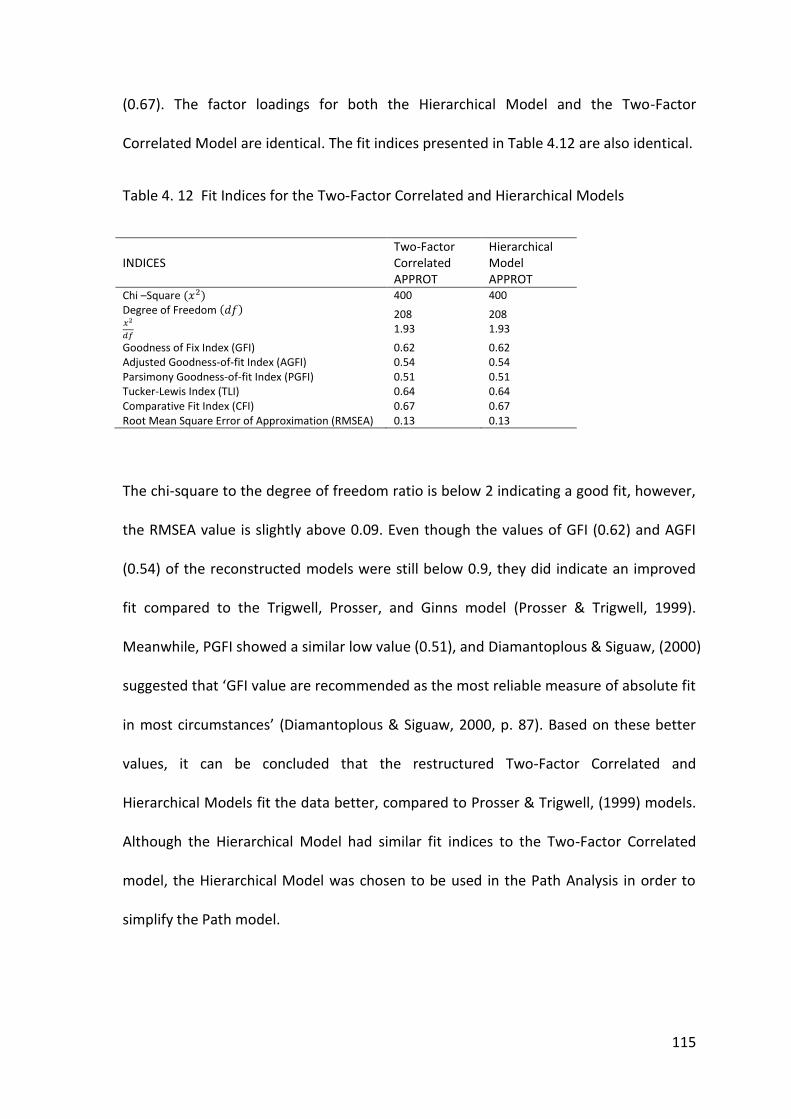
115

(0.67). The factor loadings for both the Hierarchical Model and the Two-Factor

Correlated Model are identical. The fit indices presented in Table 4.12 are also identical.

Table 4. 12 Fit Indices for the Two-Factor Correlated and Hierarchical Models

INDICES Two-Factor Correlated APPROT

Hierarchical Model APPROT

Chi –Square 400 400 Degree of Freedom

208 1.93

208 1.93

Goodness of Fix Index (GFI) 0.62 0.62 Adjusted Goodness-of-fit Index (AGFI) 0.54 0.54 Parsimony Goodness-of-fit Index (PGFI) 0.51 0.51 Tucker-Lewis Index (TLI) 0.64 0.64 Comparative Fit Index (CFI) 0.67 0.67 Root Mean Square Error of Approximation (RMSEA) 0.13 0.13

The chi-square to the degree of freedom ratio is below 2 indicating a good fit, however,

the RMSEA value is slightly above 0.09. Even though the values of GFI (0.62) and AGFI

(0.54) of the reconstructed models were still below 0.9, they did indicate an improved

fit compared to the Trigwell, Prosser, and Ginns model (Prosser & Trigwell, 1999).

Meanwhile, PGFI showed a similar low value (0.51), and Diamantoplous & Siguaw, (2000)

suggested that ‘GFI value are recommended as the most reliable measure of absolute fit

in most circumstances’ (Diamantoplous & Siguaw, 2000, p. 87). Based on these better

values, it can be concluded that the restructured Two-Factor Correlated and

Hierarchical Models fit the data better, compared to Prosser & Trigwell, (1999) models.

Although the Hierarchical Model had similar fit indices to the Two-Factor Correlated

model, the Hierarchical Model was chosen to be used in the Path Analysis in order to

simplify the Path model.

116

4.6 History Teaching Method (HTEAM) Instrument

This instrument consisted of 19 items which reflected the History teaching methods

used in Malaysian classrooms. This questionnaire was developed by the researcher,

based on the literature review of pedagogical methods used by the History teacher in

the classroom. There were two subscales in the instrument; active and effective

teaching. Active teaching consisted of 7 items (HTEAM1 to HTEAM7). Effective teaching

consisted of 12 items (HTEAM 8 to HTEAM 19). Each item used a five-point scale: 1.

Never 2. Seldom 3. Sometime 4. Often 5. Very Often. The subscales of HTEAM are

presented in Table 4.13. All the items in the questionnaire were subject to the reliability

analysis. Sekaran (1992), claimed that reliability measurement indicated the stability

and consistency with which scores were obtained from an instrument. In this study,

Cronbach Alpha was used to examine the internal consistency of the questionnaires. Yu

(n.d.) defined Cronbach Alpha as ‘a measure of squared correlation between observed

score and true score’. Cronbach Alpha indicates the internal consistency of a

questionnaire. The value of Cronbach‘s Alpha for scale of the teachers’ samples was 0.9.

117

Table 4. 13 HTEAM instrument subscale

Subscales Items

In teaching History in your classroom how often do you do the following activities?

ActTea 1 Role play/ Drama.

2 Classroom Discussion.

3 Debate.

4 Student Presentation.

5 Group work.

6 Project work.

7 Field Trips.

EffTea 8 I know how to select and structure historical knowledge for instructional purposes.

9 I know how to use a wide range of strategies and approaches for representing history.

10 I know how to use historical knowledge to foster critical thinking.

11 I teach history as possible interpretations of the past rather than as fact.

12 During a history lesson I involve students in working with raw materials (newspaper, photographs, political cartoon, letters, etc).

13 I require students to connect and relate various pieces of evidence to build images of the past

14 I provide students with opportunities to practise critical thinking skills likes (e.g.; document-based questioning).

15 I teach students to analyse primary and secondary source documents during history class.

16 I encourage students to use tools of inquiry such as interrogation, analysis, and interpretation.

17 I Introduce students to investigative processes and skills of handling, reading, and evaluating evidence.

18 I am aware that learning history is a social activity through which students learn from each other.

19 I recognise that gradually building the context for history inquiry is essential for learning.


Confirmatory Factor Analysis of the Initial Model

The Two-Factor Correlated Model was tested with CFA. The initial instrument had 19

items and two sub-scales, namely the EffTea (Effective Teaching) and the ActTea (Active

Teaching) subscales as presented in Table 4.13. CFA was used to examine how well the

observed variables were measuring the latent variables as indicated by the instrument.

The results of CFA are displayed in Tables 4.14 and 4.15. The factor structure is

presented in Figure 4.8; the factor loadings and the fit indices are presented in Tables

4.15 and 4.16.

118


Table 4. 14 Factor Loadings of Two-Factor Correlation Initial Structure

Item no. Sub-scale Factor Loadings

HTEAM1 ActTea 0.51 HTEAM2 0.60 HTEAM3 0.48 HTEAM4 0.78 HTEAM5 0.72 HTEAM6 0.63 HTEAM7 0.63 HTEAM8 EffTea 0.70 HTEAM9 0.76 HTEAM10 0.71 HTEAM11 0.58 HTEAM12 0.65 HTEAM13 0.73 HTEAM14 0.69 HTEAM15 0.70 HTEAM16 0.61 HTEAM17 0.58 HTEAM18 0.59 HTEAM19 0.56

ActiveTeaching

.26

HTEAM1 e1

.51.36

HTEAM2 e2

.60 .24

HTEAM3 e3.48.61

HTEAM4 e4.78

.52

HTEAM5 e5

.72

.40

HTEAM6 e6

.63

.40

HTEAM7 e7

.63

EffectiveTeaching

.49

HTEAM8 e8

.70

.58

HTEAM9 e9

.76

.50

HTEAM10 e10

.71

.34

HTEAM11 e11

.58.42

HTEAM12 e12.65

.54

HTEAM13 e13.73.47

HTEAM14 e14

.69

.49

HTEAM15 e15

.70

.38

HTEAM16 e16

.61

.34

HTEAM17 e17

.58

.34

HTEAM18 e18

.59

.32

HTEAM19 e19

.56

.70

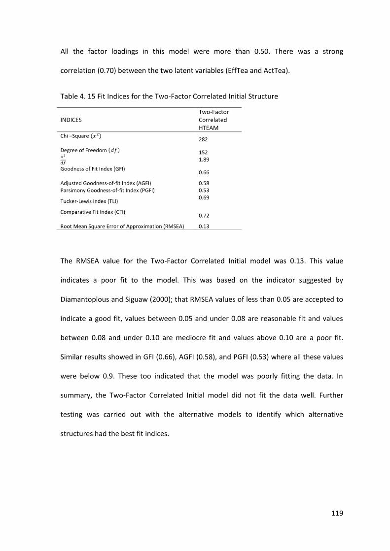
119

All the factor loadings in this model were more than 0.50. There was a strong

correlation (0.70) between the two latent variables (EffTea and ActTea).

Table 4. 15 Fit Indices for the Two-Factor Correlated Initial Structure

The RMSEA value for the Two-Factor Correlated Initial model was 0.13. This value

indicates a poor fit to the model. This was based on the indicator suggested by

Diamantoplous and Siguaw (2000); that RMSEA values of less than 0.05 are accepted to

indicate a good fit, values between 0.05 and under 0.08 are reasonable fit and values

between 0.08 and under 0.10 are mediocre fit and values above 0.10 are a poor fit.

Similar results showed in GFI (0.66), AGFI (0.58), and PGFI (0.53) where all these values

were below 0.9. These too indicated that the model was poorly fitting the data. In

summary, the Two-Factor Correlated Initial model did not fit the data well. Further

testing was carried out with the alternative models to identify which alternative

structures had the best fit indices.

INDICES Two-Factor Correlated HTEAM

Chi –Square

282

Degree of Freedom 152 1.89

Goodness of Fit Index (GFI)

0.66

Adjusted Goodness-of-fit Index (AGFI) 0.58 Parsimony Goodness-of-fit Index (PGFI) 0.53

Tucker-Lewis Index (TLI) 0.69


0.72

Root Mean Square Error of Approximation (RMSEA) 0.13

120

Exploratory Factor Analysis (EFA) of the Initials Models

Since this instrument was developed by the researcher, Exploratory Factor Analysis (EFA)

was conducted to tease out the possible groupings of the items. In addition CFA was

also implemented to confirm the structure of the instrument. According to Curtis (2005,

p.183), EFA is used to ‘show the patterns of response to the items of the instrument

reflect the constructs that were used in framing the instrument’. In this study EFA was

employed, using principal components extraction, followed by varimax rotation, using

SPSS version 17.

Table 4. 16 Rotated factor solution for an exploratory analysis of the HTEAM

Item no. Sub-scale Factor 1 Factor 2

HTEAM1 EffTea 0.46 HTEAM8 0.60 HTEAM9 0.56 HTEAM10 0.77 HTEAM11 0.72 HTEAM12 0.68 HTEAM13 0.68 HTEAM14 0.66 HTEAM15 0.58 HTEAM18 0.67 HTEAM19 0.70 HTEAM2 ActTea 0.72 HTEAM3 0.51 HTEAM4 0.79 HTEAM5 0.69 HTEAM6 0.65 HTEAM7 0.58 HTEAM16 0.65 HTEAM17 0.62

Factor loadings for the HTEAM instrument are presented in Table 4.16. The magnitude

of the factor loadings indicate that the items moderately reflected the subscales that

they were intended to reflect. However, there were a few exceptions in these results.

121

Item HTEAM1 was planned as an ActTea (Active Teaching) item, but loaded into EffTea

(Effective Teaching) scale instead. The item referred to feedback on the active teaching

that teacher would implement in the classroom (Taylor & Young, 2003). Items HTEAM16

and HTEAM17 which were initially designed to be part of the EffTea (Effective Teaching)

sub-scale had loadings of moderate size onto the ActTea (Active Teaching) sub-scale.

Overall, this analysis showed a satisfactory pattern of loadings, suggesting that most of

the items reflected the constructs that were claimed by Taylor and Young (2003) to

form the History teaching methods used in the classroom.

Although EFA showed that most of the items did reflect the constructs concerned and

that the instrument itself had coverage of the items that were implicated in History

teaching methods, EFA has its own limitations. Curtis (2005, p. 185) pointed out that

EFA fails to show the constructs that form a certain concept. He added that ‘in varimax

factor solution, each extracted factor is orthogonal to the others and therefore EFA

does not provide a basis for arguing that the identified constructs form a

unidimensional construct that is a the basis of true measurement’. Due to these

limitations, CFA was carried out further in this study to determine the structure of the

constructs.

Confirmatory Factor Analysis of the Alternative Model

EFA was carried out in order ‘to explore possible underlying structure of a set of

observed variables without imposing any preconceived structure on the outcome and

by performing EFA, the numbers of constructs and underlying factors are identified’

(Child, 1990, cited in Suhr , 2006 p. 2). Using constructs from the EFA, four models were

tested as alternative models namely; a) One Factor Model, (b) Two Factor Orthogonal

122

Model, (c) Two Factor Correlated Model and, (d) Two Factor Hierarchical Models (see

Figure 4.9). AMOS 17 was used to carry out the CFA and to draw the factor structures.

Two out of four alternative models, are discussed in this section: the Two-Factor

Correlated and Two-Factor Hierarchical models due to the high values of the factor

loadings and the values of the fit indices.

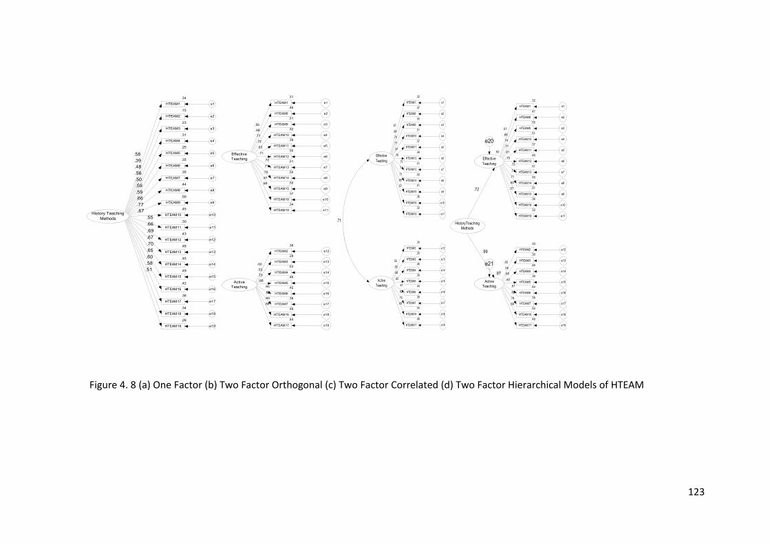
123

Figure 4. 8 (a) One Factor (b) Two Factor Orthogonal (c) Two Factor Correlated (d) Two Factor Hierarchical Models of HTEAM

History TeachingMethods

.34

HTEAM1 e1

.58

.15

HTEAM2 e2

.39

.23

HTEAM3 e3

.48

.31

HTEAM4 e4

.56

.25

HTEAM5 e5

.50

.35

HTEAM6 e6

.59

.35

HTEAM7 e7

.59

.44

HTEAM8 e8

.66 .59

HTEAM9 e9.77.45

HTEAM10 e10.67

.30

HTEAM11 e11

.55

.43

HTEAM12 e12

.66

.48

HTEAM13 e13

.69

.45

HTEAM14 e14

.67

.49

HTEAM15 e15

.70

.42

HTEAM16 e16

.65

.36

HTEAM17 e17

.60

.34

HTEAM18 e18

.58

.26

HTEAM19 e19

.51

EffectiveTeaching

.31

HTEAM1 e1

.56

.46

HTEAM8 e2

.68

.51

HTEAM9 e3

.71

.52

HTEAM10 e4

.72 .39

HTEAM11 e5.63.50

HTEAM12 e6.71

.51

HTEAM13 e7

.72

.50

HTEAM14 e8

.71

.50

HTEAM15 e9

.70

.37

HTEAM18 e10

.61

.34

HTEAM19 e11

.58

ActiveTeaching

.36

HTEAM2 e12.28

HTEAM3 e13.53

HTEAM4 e14.46

HTEAM5 e15.42

HTEAM6 e16.36

HTEAM7 e17.48

HTEAM16 e18.44

HTEAM17 e19

.60

.53

.73

.68

.65

.60

.69

.66

EffectiveTeaching

.32

HTEAM1 e1

.57

.47

HTEAM8 e2

.68

.55

HTEAM9 e3

.74

.51

HTEAM10 e4

.71 .37

HTEAM11 e5.61.49

HTEAM12 e6.70

.51

HTEAM13 e7

.72

.50

HTEAM14 e8

.71

.51

HTEAM15 e9

.71

.36

HTEAM18 e10

.60

.32

HTEAM19 e11

.57

ActiveTeaching

.30

HTEAM2 e12.30

HTEAM3 e13.46

HTEAM4 e14.39

HTEAM5 e15.44

HTEAM6 e16.39

HTEAM7 e17.54

HTEAM16 e18.48

HTEAM17 e19

.55

.55

.68

.63

.67

.62

.74

.69

.71

.52

EffectiveTeaching

.32

HTEAM1 e1

.57

.47

HTEAM8 e2

.68

.55

HTEAM9 e3

.74

.51

HTEAM10 e4

.71 .37

HTEAM11 e5.61.49

HTEAM12 e6.70

.51

HTEAM13 e7

.72

.50

HTEAM14 e8

.71

.51

HTEAM15 e9

.71

.36

HTEAM18 e10

.60

.32

HTEAM19 e11

.57

.97

ActiveTeaching

.30

HTEAM2 e12.30

HTEAM3 e13.46

HTEAM4 e14.39

HTEAM5 e15.44

HTEAM6 e16.39

HTEAM7 e17.54

HTEAM16 e18.48

HTEAM17 e19

.55

.55

.68

.63

.67

.62

.74

.69

HistoryTeachingMethods

.72

.99

e20

e21

124

The instrument consisted of 19 items; EffTea (Effective Teaching) had 11 items and

ActTea (Active Teaching) had 8 items. The Two-Factor Correlated Model was tested to

determine the fit of the hypothesis model to the sample data. The results of CFA are

displayed in the factor loadings table (Table 4.17) and in the fit indices table (Table 4.18).

The factor structure is presented in Figure 4.10.


EffectiveTeaching

.32

HTEAM1 e1

.57

.47

HTEAM8 e2

.68

.55

HTEAM9 e3

.74

.51

HTEAM10 e4

.71 .37

HTEAM11 e5.61.49

HTEAM12 e6.70

.51

HTEAM13 e7

.72

.50

HTEAM14 e8

.71

.51

HTEAM15 e9

.71

.36

HTEAM18 e10

.60

.32

HTEAM19 e11

.57

ActiveTeaching

.30

HTEAM2 e12.30

HTEAM3 e13.46

HTEAM4 e14.39

HTEAM5 e15.44

HTEAM6 e16.39

HTEAM7 e17.54

HTEAM16 e18.48

HTEAM17 e19

.55

.55

.68

.63

.67

.62

.74

.69

.71

125

Table 4. 17 Factor Loadings of Two-Factor Correlated (New Structure) and Hierarchical Model

Item no. Sub-scale Two – Factor Correlated Model

Hierarchical Model

Factor 1 Factor 2 Factor 1

Factor 2

HTEAM1 EffTea 0.46 0.57

HTEAM8 0.60 0.68

HTEAM9 0.56 0.74

HTEAM10 0.77 0.71

HTEAM11 0.72 0.61

HTEAM12 0.68 0.70

HTEAM13 0.68 0.72

HTEAM14 0.66 0.71

HTEAM15 0.58 0.71

HTEAM18 0.67 0.60

HTEAM19 0.70 0.57

HTEAM2 ActTea 0.72 0.55 HTEAM3 0.51 0.55 HTEAM4 0.79 0.68 HTEAM5 0.69 0.63 HTEAM6 0.65 0.67 HTEAM7 0.58 0.62 HTEAM16 0.65 0.74 HTEAM17 0.62 0.69

The loadings for the Two-Factor Correlated and Hierarchical Models as presented in

Table 4.17 ranged from 0.46 to 0.79, showing that the items moderately reflected the

latent variable. The correlation between the two latent variables (EffTea and ActTea) is

high (r=0.71). The correlation coefficient, for this model were slightly higher compared

to the Two-Factor Initial model (0.70). The loadings for the Hierarchical Model showed

the same values as the Two-Factor Correlated Model. In summary, these models, to

some extent, are improvement to the initial models. The fit indices of Two-Factor

Correlated and Hierarchical Models are presented in Table 4.18.

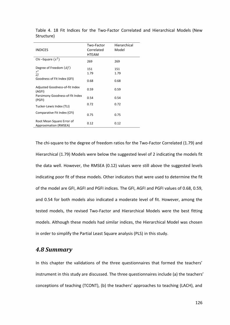
126

Table 4. 18 Fit Indices for the Two-Factor Correlated and Hierarchical Models (New Structure)

INDICES Two-Factor Correlated HTEAM

Hierarchical Model

Chi –Square

269 269

Degree of Freedom

151 1.79

151 1.79

Goodness of Fit Index (GFI)

0.68 0.68

Adjusted Goodness-of-fit Index (AGFI)

0.59 0.59

Parsimony Goodness-of-fit Index (PGFI)

0.54 0.54


0.72


0.75 0.75


0.12 0.12

The chi-square to the degree of freedom ratios for the Two-Factor Correlated (1.79) and

Hierarchical (1.79) Models were below the suggested level of 2 indicating the models fit

the data well. However, the RMSEA (0.12) values were still above the suggested levels

indicating poor fit of these models. Other indicators that were used to determine the fit

of the model are GFI, AGFI and PGFI indices. The GFI, AGFI and PGFI values of 0.68, 0.59,

and 0.54 for both models also indicated a moderate level of fit. However, among the

tested models, the revised Two-Factor and Hierarchical Models were the best fitting

models. Although these models had similar indices, the Hierarchical Model was chosen

in order to simplify the Partial Least Square analysis (PLS) in this study.

4.8 Summary

In this chapter the validations of the three questionnaires that formed the teachers’

instrument in this study are discussed. The three questionnaires include (a) the teachers’

conceptions of teaching (TCONT), (b) the teachers’ approaches to teaching (LACH), and

127

(c) the teachers’ History teaching methods (HTEAM). Each questionnaire underwent the

same validation procedures using Confirmatory Factor Analysis (CFA) and Exploratory

Factor Analysis (EFA). Two sets of models were discussed in detail for all questionnaires:

the Baseline Confirmatory and Alternative Models. CFA considered factor loadings and

model fit indices. All instruments were tested to determine if the model fitted the

sample data. Finally, in each case one of the alternative models which had the best fit

was selected for further analysis. Across the three questionnaires of the teachers’

instrument, the models chosen for further study were as follow:

1. The Teachers’ Approaches to Teaching scale were applied in this study to assess

teachers’ conception of teaching in order to discover the relations of conceptions

and student learning Goa & Watkins, (2002). After examining the CFA results of all

the alternative models, it was decided to use the Hierarchical Model in subsequent

analysis in this research.

2. The Approaches to Teaching Inventory (ATI - 22) was used to measure the

relationship between students’ approaches to learning and teachers’ approaches to

teaching (Prosser et al., 2006). The Hierarchical Model was chosen for the further

analysis.

3. The History Teaching Method (HTEAM) Instrument was developed by the

researcher to investigate the History teaching methods used in the classroom.

Based on both EFA and CFA analyses, it was decided to use the Hierarchical Model

in subsequent analysis.

128

Chapter 5 Validation of the Research

Instruments: Students’ ________________________________________________________________________

5.1 Introduction

This chapter continues the validity and reliability testing of the instruments used in this

study. The students’ instrument was tested using Confirmatory Factor Analysis (CFA) to

examine its construct validity, while the internal consistency was measured with the

Cronbach’s Alpha coefficient. The analyses were based on data collected from 1653

students studying History in secondary schools across Kuala Lumpur.

The students’ questionnaire comprised of four sections. Section 1 collected respondents’

personal information. Section 2 of the questionnaire was designed to gather

information on their History classroom climate (ICEQ). Section 3 was used to explore

students’ learning process (LPQ). In section 4, students’ perception towards learning

History (SPERCH) was the focus of inquiry.

Model Fit Indices

The results from the CFA analyses provided various fit indices such as the Mean Square

Error of Approximation (RMSEA), the Tucker-Lewis Index (TLI), and the Comparative Fit

Index (CFI). According to Ben (2010, p. 100), these indices ‘assess how well the samples’

covariance were reproduced by the covariance are predicted from the parameter

estimates’. A value from RMSEA shows ‘how well would the model, with unknown but

optimally chosen parameter values, fit the population covariance matrix if it were

available’ (Diamantoplous & Siguaw, 2000, p. 85). Values of RMSEA less than 0.05 are

129

accepted to indicate a good fit, values between 0.05 and 0.08 indicate a reasonable fit

values between 0.08 and under 0.10 a mediocre fit and values lower than 0.10 show a

poor fit (Diamantoplous & Siguaw, 2000). Other indicators used in this study were CFI

and TLI, where values greater than or equal to 0.90 reveal good fit to the data. The CFI,

TLI and RMSEA values are preferred by many researchers for a one time analysis

(Schreiber, et al. 2006).

Besides the goodness of fit indicators mentioned above, chi-square divided by the

number of degrees of freedom is also used as an indicator of goodness-of-fit in this

study. Al-Gahtani and King (1999, cited in Darmawan 2003, p. 96) added that ‘values of

the chi-square to the number of degree of freedom of less than 5 for a larger model can

be considered an indicator of a good fit’. Other indices that can be used are GFI, AGFI

and PGFI. However, since the students’ data missing values, these indices were not

provided as part of AMOS output. The summary of the fit indexes used for the students’

instrument is presented in Table 5.1.

Table 5. 1 Summary of fit indices used in validation of the scales in students’ instruments

Fix Index Values to indicate Good Fit

Root Mean Square Error of Approximation (RMSEA) ≤0.05

Comparative fit index (CFI) ≥ 0.90

Tucker-Lewis Index (TLI) ≥ 0.90

< 5

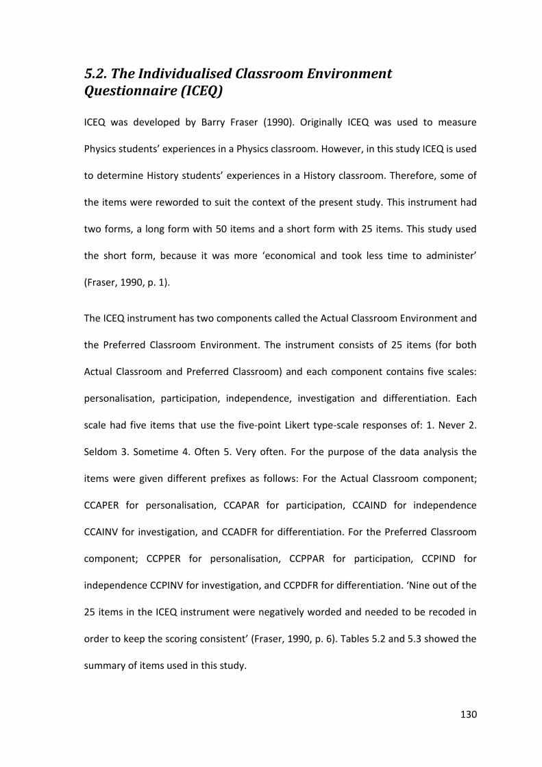
130

5.2. The Individualised Classroom Environment Questionnaire (ICEQ)

ICEQ was developed by Barry Fraser (1990). Originally ICEQ was used to measure

Physics students’ experiences in a Physics classroom. However, in this study ICEQ is used

to determine History students’ experiences in a History classroom. Therefore, some of

the items were reworded to suit the context of the present study. This instrument had

two forms, a long form with 50 items and a short form with 25 items. This study used

the short form, because it was more ‘economical and took less time to administer’

(Fraser, 1990, p. 1).

The ICEQ instrument has two components called the Actual Classroom Environment and

the Preferred Classroom Environment. The instrument consists of 25 items (for both

Actual Classroom and Preferred Classroom) and each component contains five scales:

personalisation, participation, independence, investigation and differentiation. Each

scale had five items that use the five-point Likert type-scale responses of: 1. Never 2.

Seldom 3. Sometime 4. Often 5. Very often. For the purpose of the data analysis the

items were given different prefixes as follows: For the Actual Classroom component;

CCAPER for personalisation, CCAPAR for participation, CCAIND for independence

CCAINV for investigation, and CCADFR for differentiation. For the Preferred Classroom

component; CCPPER for personalisation, CCPPAR for participation, CCPIND for

independence CCPINV for investigation, and CCPDFR for differentiation. ‘Nine out of the

25 items in the ICEQ instrument were negatively worded and needed to be recoded in

order to keep the scoring consistent’ (Fraser, 1990, p. 6). Tables 5.2 and 5.3 showed the

summary of items used in this study.

131

Table 5. 2 Summary of ICEQ items used in the Students’ Questionnaire (Actual Classroom)

Item Code Nature of Statement

Item code to indicate Reverse scoring

Item statement

CCAPER1 Positive None The teacher talks with each student.

CCAPAR2 Positive None Students give their opinions during discussions

CCAIND3 Negative CCAIND3R The teacher decides where students sit.

CCAINV4 Negative CCAINV4R Students find out the answers to questions from textbooks rather than from history inquiry.

CCADFR5 Positive None Different students do different work.

CCAPER6 Positive None The teacher takes a personal interest in each student

CCAPAR7 Negative CCAPAR7R The teacher lectures without students asking or answering questions.

CCAIND8 Positive None Students choose their partners for group work.

CCAINV9 Positive None Students carry out history inquiry to check evidence

CCADFR10 Negative CCADFR10R All students in the class do the same work at the same time

CCAPER11 Negative CCAPER11R The teacher is unfriendly to students.

CCAPAR12 Positive None Students’ ideas and suggestions are used during classroom discussion

CCAIND13 Negative CCAIND13R Students are told how to behave in the classroom

CCAINV14 Positive None Students carry out history inquiry to answer questions coming from class discussions.

CCADFR15 Positive None Different students use different books and materials.

CCAPER16 Positive None The teacher helps each student who is having trouble with the work

CCAPAR17 Positive None Students ask the teacher questions.

CCAIND18 Negative CCAIND18R The teacher decides which students should work together.

CCAINV19 Positive None Students explain the meanings of statements and time line.

CCADFR20 Positive None Students who work faster than others move on to the next topic.

CCAPER21 Positive None The teacher considers students’ feelings.

CCAPAR22 Positive None There is classroom discussion

CCAIND23 Negative CCAIND23R The teacher decides how much movement and talk there should be in the classroom.

CCAINV24 Positive None Students carry out history inquiry to answer questions which puzzle them.

CCADFR25 Negative CCADFR25R The same teaching aid (e.g. blackboard or overhead projector) is used for all students in the class.

132

Table 5. 3 Summary of ICEQ items used in the Students’ Questionnaire (Preferred Classroom)

Item Code Nature of Statement

Item code to indicate Reverse scoring

Item statement

CCPPER1 Positive None The teacher would talk with each student.

CCPPAR2 Positive None Students would give their opinions during discussions

CCPIND3 Negative CCPIND3R The teacher would decide where students sit.

CCPINV4 Negative CCPINV4R Students would find out the answers to questions from textbooks rather than from history inquiry.

CCPDFR5 Positive None Different students would do different work.

CCPPER6 Positive None The teacher would takes a personal interest in each student

CCPPAR7 Negative CCPPAR7R The teacher would lecture without students asking or answering questions.

CCPIND8 Positive None Students would choose their partners for group work.

CCPINV9 Positive None Students would carry out history inquiry to check evidence

CCPDFR10 Negative CCPDFR10R All students in the class would do the same work at the same time

CCPPER11 Negative CCPPER11R The teacher would be unfriendly to students.

CCPPAR12 Positive None Students’ ideas and suggestions would be used during classroom discussion

CCPIND13 Negative CCPIND13R Students would be told how to behave in the classroom

CCPINV14 Positive None Students would carry out history inquiry to answer questions coming from class discussions.

CCPDFR15 Positive None Different students would use different books and materials.

CCPPER16 Positive None The teacher would help each student who is having trouble with the work

CCPPAR17 Positive None Students would ask the teacher questions.

CCPIND18 Negative CCPIND18R The teacher would decide which students should work together.

CCPINV19 Positive None Students would explain the meanings of statements and time line.

CCPDFR20 Positive None Students who work faster than others move on to the next topic.

CCPPER21 Positive None The teacher would consider students’ feelings.

CCPPAR22 Positive None There would be classroom discussion

CCPIND23 Negative CCPIND23R The teacher decides would how much movement and talk there should be in the classroom.

CCPINV24 Positive None Students would carry out history inquiry to answer questions which puzzle them.

CCPDFR25 Negative CCPDFR25R The same teaching aid (e.g. blackboard or overhead projector) is used for all students in the class.

133

ICEQ is widely used in several different countries and for different purposes. Fraser

(p. 16, 1990) explained in the ICEQ Handbook that ICEQ had been tested in a few

countries, using cross-validation procedures. The findings from the cross-validation data

from Australia, Indonesia, and the Netherlands demonstrated the internal consistency

and scale independence of both forms (long and short) of the ICEQ instrument. For the

short form, the alpha coefficients range between 0.63 to 0.85. Fraser added that the

results indicated that the reliability of the short form of a scale was typically

approximately 0.1 smaller that the reliability of the corresponding long form. According

to Fraser, these results reflected that the short form component had a satisfactory

reliability based on the class mean. As for the correlation of the five scales, the findings

showed values ranging from 0.13 to 0.36. These value indicated that the short form had

an adequate level of scale independence. For the test-retest reliability coefficient, the

five scales of ICEQ were: Personalisation (0.78), Participation (0.67), Independence

(0.83), Investigation (0.75) and Differentiation (0.78). These results indicated that ICEQ

had satisfactory reliability. The following section discusses in detail the ICEQ instrument

validation using CFA.


The CFA modeling was based on the sample of 1653 students from this study. AMOS 17

(Arbuckle, 2008) was used to carry out CFA and for drawing the structure diagrams in

this analysis. CFA was carried out to test the existing models and, subsequently, a

number of alternative models in order to determine the best fitting model.

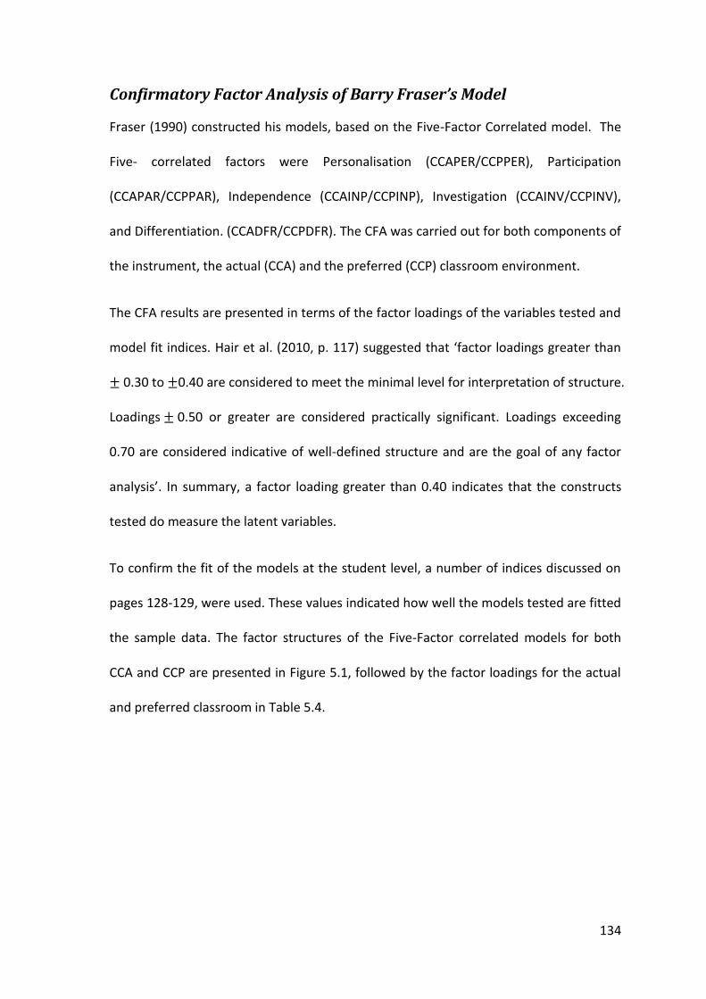
134

Confirmatory Factor Analysis of Barry Fraser’s Model

Fraser (1990) constructed his models, based on the Five-Factor Correlated model. The

Five- correlated factors were Personalisation (CCAPER/CCPPER), Participation

(CCAPAR/CCPPAR), Independence (CCAINP/CCPINP), Investigation (CCAINV/CCPINV),

and Differentiation. (CCADFR/CCPDFR). The CFA was carried out for both components of

the instrument, the actual (CCA) and the preferred (CCP) classroom environment.

The CFA results are presented in terms of the factor loadings of the variables tested and

model fit indices. Hair et al. (2010, p. 117) suggested that ‘factor loadings greater than

0.30 to 0.40 are considered to meet the minimal level for interpretation of structure.

Loadings 0.50 or greater are considered practically significant. Loadings exceeding

0.70 are considered indicative of well-defined structure and are the goal of any factor

analysis’. In summary, a factor loading greater than 0.40 indicates that the constructs

tested do measure the latent variables.

To confirm the fit of the models at the student level, a number of indices discussed on

pages 128-129, were used. These values indicated how well the models tested are fitted

the sample data. The factor structures of the Five-Factor correlated models for both

CCA and CCP are presented in Figure 5.1, followed by the factor loadings for the actual

and preferred classroom in Table 5.4.

135

Figure 5. 1 Five-Factor Correlated Model of CCA and CCP

Table 5. 4 Factor Loadings of Five-Factor Correlated Model for CCA and CCP

Item

PERSONALISATION PATICIPATION INDEPENDENCE INVESTIGATION DIFFERENTIATION

CCA CCP CCA CCP CCA CCP CCA CCP CCA CCP

PER1 0.53 0.48 PER6 0.23 0.16 PER11R 0.40 -0.46 PER16 0.68 0.72 PER21 0.55 0.59

PAR2 0.59 0.65 PAR7R 0.19 -0.23 PAR12 0.60 0.65 PAR17 0.50 0.60 PAR22 0.58 0.62

IND3R 0.56 0.68 IND8 0.10 -0.29 IND13R 0.28 0.35 IND18R 0.60 0.68 IND23R 0.33 0.44

INV4R 0.12 0.16 INV9 -0.64 0.65 INV14 -0.66 0.70 INV19 -0.27 0.47 INV24 -0.45 0.64

DFR5 0.43 0.44 DFR10R 0.82 -0.72 DFR15 0.19 0.14 DFR20 0.04 0.16 DFR25R 0.22 -0.41

Personalisation

.28

CCAPER1 e1

.53 .05

CCAPER6 e2.23.16

CCAPER11R e3.40

.46

CCAPER16 e4

.68

.31

CCAPER21 e5

.55

Participation

.35

CCAPAR2 e6.04

CCAPAR7R e7.36

CCAPAR12 e8.25

CCAPAR17 e9.34

CCAPAR22 e10

.59.19.60

.50

.58

Independence

.32

CCAIND3R e11.01

CCAIND8 e12.08

CCAIND13R e13.36

CCAIND18R e14.11

CCAIND23R e15

.56.10.28

.60

.33

Investigation

.01

CCAINV4R e16.41

CCPINV9 e17.44

CCPINV14 e18.07

CCAINV19 e19.20

CCAINV24 e20

.12-.64-.66

-.27-.45

Differentiation

.19

CCADFR5 e21.67

CCADFR10R e22.03

CCADFR15 e23.00

CCADFR20 e24.05

CCADFR25R e25

.43.82.19

.04

.22

.80

-.20

-.27

-.42

-.42

-.39

-.45 .32

.15

.13

Personalisation

.23CCPPER1 e1

.48 .03

CCPPER6 e2.16.21

CCPPER11R e3-.46

.52CCPPER16 e4

.72

.34

CCPPER21 e5

.59

Participation

.42CCPPAR2 e6

.05

CCPPAR7R e7.43

CCPPAR12 e8.36

CCPPAR17 e9.38

CCPPAR22 e10

.65-.23.65

.60

.62

Independence

.46CCPIND3R e11

.08

CCPIND8 e12.12

CCPIND13R e13.46

CCPIND18R e14.19

CCPIND23R e15

.68-.29.35

.68

.44

Investigation

.02CCPINV4R e16

.43CCPINV9 e17

.49

CCPINV14 e18.22

CCPINV19 e19.41

CCPINV24 e20

.16

.65.70

.47

.64

Differentiaton

.19CCPDFR5 e21

.52CCPDFR10R e22

.02

CCPDFR15 e23.03

CCPDFR20 e24.17

CCPDFR25R e25

.44-.72.14

.16-.41

.89

-.11

.55

-.70

.07

.71

-.62 .28

.00

-.44

136

The results showed that most of the factor loadings for the Five-Factor correlated model

of CCA were moderate. All of the five dimensions in ICEQ instrument had positive

loadings except for the investigation dimension, which showed a negative loading.

There were four variables that had negative values CCAINV9 (-0.64), CCAINV14 (-0.66),

CCAINV19 (-0.27) and CCAINV24 (-0.45). However, most of the absolute values were

more then 0.30, except for CCAINV19 (-0.27). Furthermore, out of 25 items, 7 items;

namely CCAPER6 (0.23), CCAPAR7R (0.17), CCAIND8 (0.10), CCAIND13R (0.28),

CCADFR20 (0.04), had factor loadings less than 0.30. These factor loadings indicate that

the items did not reflect the latent variables well. Similar results were apparent in the

actual correlation between each scale in actual classroom components.

Factor loadings for CCP, as presented in Table 5.4, ranged from -0.72 to 0.72 which

indicated strong loadings. There were a few items that had negative factor loadings

CCPER11R (-0.46), CCPPAR7R (-0.23), CCPIND8 (-0.29), CCPDFR10R (-0.72) and

CCPDFR25R (-0.41). Most of these items had an absolute factor loading of more than

0.30 except for CCPPAR7R (-0.23) and CCPIND8 (-0.29). In addition, there were four

items that had factor loadings of less than 0.30. These items were CCPINV4R (0.16),

CCPDFR15 (0.14) and CCPDFR20 (0.16). From these results it can be argued that both

components in the ICEQ instrument (actual classroom and preferred classroom) were

not fitting the sample data well, although in general items in the CCP component

showed stronger factor loadings. Some items also revealed conflicting results. While

PER11R had a positive loading for CCA, it had a negative loading for CCP. Similar results

were also found for PAR7R, IND8, DRF10R and DRF25R. These flips between negative

and positive indicate inconsistency in students’ responses for these items. For these

137

reasons, a few items were removed from both components, CCA and CCP; namely

PER11R (CCA 0.40, CCP -0.46), PAR7R (CCA 0.19, CCP -0.23), IND8 (CCA 0.10, CCP -0.29),

INV4R (CCA 0.12, CCP 0.16), DRF10R (CCA 0.82, CCP -0.72) and DRF25R (CCA 0.22, CCP -

0.41). Furthermore, four models for each component were proposed for testing as

alternative models in this study.

Table 5. 5 Fit Indices for the Five - Factor Correlated Models of ICEQ

INDICES Five-Factor Correlated (CCA)

Five-Factor Correlated (CCP)

Chi –Square 2365.43

2325.54

Degree of Freedom

265 8.93

265 8.78

Tucker-Lewis Index (TLI) 0.57 0.70 Comparative Fit Index (CFI) 0.65 0.75 Root Mean Square Error of Approximation (RMSEA)

0.07 0.07

Both models showed high chi-square values. However, this indicator is sensitive to the

sample size (Diamantoplous & Siguaw, 2000).The other alternative indicator used was

the

< 5. The results showed that the values of the

for CCA (8.93) and CCP (8.78)

were greater than 5. The results indicated that these models did not fit the data well.

Then TLI, CFI values and RMSEA were used to evaluate the goodness-of-model fit. The

RMSEA value for both components CCA and CCP in the ICEQ instrument was 0.07. This

result indicated a reasonable fit, based on the indicator suggested by Diamantoplous

and Siguaw, (2000). In addition, the values of TLI and CFI were below 0.90 for both

models. Based on the fit indices discussed above, these models needed to be improved.

Therefore, four alternative models were proposed for testing in this study.

138


Four additional models were tested as alternative models, using AMOS (Version 17).

These were; a) One Factor Model, (b) Five Factor Orthogonal Model, (c) Five Factor

Correlated Model and, (d) Five Factor Hierarchical Model (see Figures 5.2 for CCA and

5.3 for CCP). These models were tested due to the poor factor loadings and low fit

indices of the initial models.

Table 5. 6 Researcher’s New Structure Factor for CCA (Actual Classroom Environment)

Author Factor

Old Order Researcher Factor

New Order Classification

PER CCAPER1 PER CCAPER1 CCAPER6 CCAPER6 CCAPER11R CCAPER11R Removed CCAPER16 CCAPER16 CCAPER21 CCAPER21

PAR CCAPAR2 PAR CCAPAR2 CCAPAR7R CCAPAR7R Removed CCAPAR12 CCAPAR12 CCAPAR17 CCAPAR17 CCAPAR22 CCAPAR22

IND CCAIND3R IND CCAIND3R CCAIND8 CCAIND8 Removed CCAIND13R CCAIND13R CCAIND18R CCAIND18R CCAIND23R CCAIND23R

INV CCAINV4R INV CCAINV4R Removed CCAINV9 CCAINV9 CCAINV14 CCAINV14 CCAINV19 CCAINV19 CCAINV24 CCAINV24

DFR CCADFR5 DFR CCADFR5 CCADFR10R CCADFR10R Removed CCADFR15 CCADFR15 CCADFR20 CCADFR20 CCADFR25R CCADFR25R Removed

139

The new structure for the alternative models is presented in Tables 5.6 and 5.7 which

show that the five scales were retained, but a few items were removed, namely PER11R,

PAR7R, IND8, INV4R, DRF10R and DRF25R. The factor loadings of the alternative models

are presented in Table 5.8 and the factor structures for both components are presented

in Figures 5.2 and 5.3.

Table 5. 7 Researcher’s New Structure for CCP (Preferred Classroom Environment)

Author Factor

Old Order Researcher Factor

New Order Classification

PER CCPPER1 PER CCPPER1 CCPPER6 CCPPER6 CCPPER11R CCPPER11R Removed CCPPER16 CCPPER16 CCPPER21 CCPPER21

PAR CCPPAR2 PAR CCPPAR2 CCPPAR7R CCPPAR7R Removed CCPPAR12 CCPPAR12 CCPPAR17 CCPPAR17 CCPPAR22 CCPPAR22

IND CCPIND3R IND CCPIND3R CCPIND8 CCPIND8 Removed CCPIND13R CCPIND13R CCPIND18R CCPIND18R CCPIND23R CCPIND23R

INV CCPINV4R INV CCPINV4R Removed CCPINV9 CCPINV9 CCPINV14 CCPINV14 CCPINV19 CCPINV19 CCPINV24 CCPINV24

DFR CCPDFR5 DFR CCPDFR5 CCPDFR10R CCPDFR10R Removed CCPDFR15 CCPDFR15 CCPDFR20 CCPDFR20 CCPDFR25R CCPDFR25R Removed

140

Table 5. 8 Factor Loadings of the Alternative Models - CCA and CCP

CCA CCP

Items One Factor Model

Items Five-Factor Orthogonal Model

Five-Factor Correlated Model

Five-Factor Hierarchical Model

Items One Factor Model

Items Five-Factor Orthogonal Model

Five-Factor Correlated Model

Five-Factor Hierarchical Model

Loadings Loadings Loadings Loadings Loadings Loadings Loadings Loadings

CCPPER1 0.47 PER CCPPER1 0.54 0.48 0.55 CCPPER1 0.50 PER CCPPER1 0.44 0.50 0.52 CCPPAR2 0.55 CCPPER6 0.27 0.38 0.29 CCPPER6 0.64 CCPPER6 0.20 0.20 0.24 CCPDFR5 -0.05 CCPPER16 0.66 0.63 0.63 CCPPER16 -0.14 CCPPER16 0.72 0.70 0.67 CCPPER6 0.30 CCPPER21 0.53 0.54 0.53 CCPPER21 0.25 CCPPER21 0.61 0.57 0.56 CCPINV9 0.45 PAR CCPPAR2 0.63 0.59 0.61 CCPPAR2 0.53 PAR CCPPAR2 0.70 0.66 0.67 CCPPAR12 0.56 CCPPAR12 0.63 0.61 0.61 CCPPAR12 0.62 CCPPAR12 0.70 0.65 0.66 CCPINV14 0.49 CCPPAR17 0.52 0.50 0.49 CCPPAR17 0.57 CCPPAR17 0.56 0.59 0.59 CCPDFR15 0.12 CCPPAR22 0.50 0.58 0.57 CCPPAR22 0.14 CCPPAR22 0.55 0.61 0.61 CCPPER16 0.51 IND CCPIND3R 0.60 0.56 0.57 CCPIND3R 0.59 IND CCPIND3R 0.69 0.67 0.67 CCPPAR17 0.43 CCPIND13R 0.24 0.29 0.30 CCPIND13R 0.56 CCPIND13R 0.36 0.35 0.37 CCPINV19 0.35 CCPIND18R 0.57 0.57 0.56 CCPIND18R 0.44 CCPIND18R 0.66 0.66 0.65 CCPDFR20 0.18 CCPIND23R 0.34 0.35 0.34 CCPIND23R 0.05 CCPIND23R 0.45 0.46 0.46 CCPPER21 0.45 INV CCPINV9 0.64 0.64 0.62 CCPINV9 0.50 INV CCPINV9 0.68 0.66 0.67 CCPPAR22 0.56 CCPINV14 0.69 0.66 0.67 CCPINV14 0.61 CCPINV14 0.71 0.70 0.70 CCPINV24 0.48 CCPINV19 0.31 0.28 0.35 CCPINV19 0.65 CCPINV19 0.42 0.47 0.45 CCPIND3R -0.30 CCPINV24 0.58 0.45 0.60 CCPINV24 0.11 CCPINV24 0.64 0.65 0.65 CCPIND13R -0.30 DFR CCPDFR5 0.48 0.47 0.41 CCPDFR5 0.20 DFR CCPDFR5 0.53 0.50 0.55 CCPIND18 -0.32 CCPDFR15 0.62 0.58 0.72 CCPDFR15 0.13 CCPDFR15 0.57 0.51 0.55 CCPIND23R -0.20 CCPDFR20 0.26 0.32 0.25 CCPDFR20 0.23 CCPDFR20 0.46 0.54 0.45

141

Figure 5. 2 (a) One Factor (b) Five Factor Orthogonal (c) Five Factor Correlated (d) Five Factor Hierarchical Models of CCA

CCA

.22

CCAPER1 e1

.47

.30

CCAPAR2 e2

.55

.00

CCADFR5 e3

-.05

.09

CCAPER6 e4

.30

.20

CCAINV9 e5

.45

.31

CCAPAR12 e6

.56

.24

CCAINV14 e7

.49.02

CCADFR15 e8.12 .26

CCAPER16 e9.51.19

CCAPAR17 e10

.43

.12

CCAINV19 e11

.35

.03

CCADFR20 e12

.18

.20

CCAPER21 e13

.45

.31

CCAPAR22 e14

.56

.23

CCAINV24 e15

.48

.09

CCAIND3R e16

-.30

.09

CCAIND13R e17

-.30

.10

CCAIND18R e18

-.32

.04

CCAIND23R e19

-.20

Personalisation

.29

CCAPER1 e1.54.07

CCAPER6 e2.27

.44

CCAPER16 e3

.66

.28

CCAPER21 e4

.53

Participation

.40

CCAPAR2 e5.40

CCAPAR12 e6.27

CCAPAR17 e7.25

CCAPAR22 e8

.63.52.50

Independence

.36

CCAIND3R e9

.06

CCAIND13R e10.32

CCAIND18R e11.12

CCAIND23R e12

.24.57.34

Investigation

.41

CCAINV9 e13.47

CCAINV14 e14.10

CCAINV19 e15.34

CCAINV24 e16

.64.69

.31

.58

Differentiation

.23

CCADFR5 e17.38

CCADFR15 e18.07

CCADFR20 e19

.62

.26

.63

.60

.48

Personalisation

.23

CCAPER1 e1.48 .14

CCAPER6 e2.38.40

CCAPER16 e3

.63

.29

CCAPER21 e4

.54

Participation

.35

CCAPAR2 e5.37

CCAPAR12 e6.25

CCAPAR17 e7.34

CCAPAR22 e8

.58

Independence

.31

CCAIND3R e9

.08

CCAIND13R e10.33

CCAIND18R e11.12

CCAIND23R e12

.56.29

.57

.35

Investigation

.41

CCPINV9 e13.43

CCPINV14 e14.08

CCAINV19 e15.21

CCAINV24 e16

.64.66

.28

.45

Differentiation

.22

CCADFR5 e17.34

CCADFR15 e18.10

CCADFR20 e19

.58.32

.82

-.34

.29

.00

-.46

.39

.06 -.33

-.27

.26

.47

.50

.59.61

.68

Personalisation

.31

CCAPER1 e1.55.09

CCAPER6 e2.29

.40

CCAPER16 e3

.63

.28

CCAPER21 e4

.53

.93

Participation

.37

CCAPAR2 e5

.37

CCAPAR12 e6.24

CCAPAR17 e7.33

CCAPAR22 e8

.61.61

.49

.57

.25

Independence

.32

CCAIND3R e9

.09

CCAIND13R e10.32

CCAIND18R e11.12

CCAIND23R e12

.57.30

.56

.34

.39

Investigation

.38

CCAINV9 e13.45

CCAINV14 e14.13

CCAINV19 e15.36

CCAINV24 e16

.62.67

.35

.60

.02

Differentiation

.16

CCADFR5 e17

.52

CCADFR15 e18.06

CCADFR20 e19

.41.72

.25

ClassroomClimate Actual

.82

.96

-.50

.63

.13

e20

e21

e22

e23

e24

142

Figure 5. 3 (a) One Factor (b) Five Factor Orthogonal (c) Five Factor Correlated Models (d) Five Factor Hierarchical Models of CCP

CCP

.25

CCPPER1 e1

.50

.41

CCPPAR2 e2

.64

.02

CCPDFR5 e3

-.14

.06

CCPPER6 e4

.25

.28

CCPINV9 e5

.53

.38

CCPPAR12 e6

.62

.33

CCPINV14 e7

.57

.02

CCPDFR15 e8

.14.34

CCPPER16 e9.59.31

CCPPAR17 e10.56

.20

CCPINV19 e11

.44

.00

CCPDFR20 e12

.05

.25

CCPPER21 e13

.50

.37

CCPPAR22 e14

.61

.30

CCPINV24 e15

.55

.01

CCPIND3R e16

.11

.04

CCPIND13R e17.02

CCPIND18R e18

.13

.05

CCPIND23R e19

.23

.20

Personalisation

.19

CCPPER1 e1.44.04

CCPPER6 e2.20

.51CCPPER16 e3

.72

.38

CCPPER21 e4

.61

Participation

.48CCPPAR2 e5

.50CCPPAR12 e6

.31

CCPPAR17 e7.30

CCPPAR22 e8

.70.70

.56

.55

Independence

.47CCPIND3R e9

.13CCPIND13R e10

.43CCPIND18R e11

.20CCPIND23R e12

.69.36

.66

.45

Investigation

.47CCPINV9 e13

.51

CCPINV14 e14.17

CCPINV19 e15.41

CCPINV24 e16

.68

.71.42.64

Differentiaton

.28CCPDFR5 e17

.32

CCPDFR15 e18.21

CCPDFR20 e19

.53.57

.46

Personalisation

.25CCPPER1 e1.50

.04CCPPER6 e2

.20.48

CCPPER16 e3

.70

.33

CCPPER21 e4

.57

Participation

.43CCPPAR2 e5

.42CCPPAR12 e6

.35CCPPAR17 e7

.38CCPPAR22 e8

.66

.65.59.61

Independence

.44CCPIND3R e9

.12CCPIND13R e10

.44CCPIND18R e11

.22CCPIND23R e12

.67.35

.66

.46

Investigation

.43CCPINV9 e13

.49CCPINV14 e14

.22CCPINV19 e15

.42CCPINV24 e16

.66.70

.47

.65

Differentiaton

.25CCPDFR5 e17

.26CCPDFR15 e18

.29CCPDFR20 e19

.50.51.54

.93

.02

.59

-.17

.14

.71

-.06 .32

.32

.22

.85

Personalisation

.27

CCPPER1 e1.52.06

CCPPER6 e2.24

.45

CCPPER16 e3

.67

.32CCPPER21 e4

.56

.98

Participation

.45

CCPPAR2 e5.43

CCPPAR12 e6.35

CCPPAR17 e7.38

CCPPAR22 e8

.67.66

.59

.61

.02

Independence

.45CCPIND3R e9

.14

CCPIND13R e10.42

CCPIND18R e11.21

CCPIND23R e12

.67.37

.65

.46

.48

Investigation

.44

CCPINV9 e13.49

CCPINV14 e14.20

CCPINV19 e15.42

CCPINV24 e16

.67.70

.45.65

.00

Differentiaton

.31

CCPDFR5 e17.30

CCPDFR15 e18.21

CCPDFR20 e19

.55.55

.45

ClassroomClimate Preferred

.92

.99

.16

.69

-.05

e20

e21

e22

e23

e24

143

Factor loadings of the four models, namely the One Factor Model, the Five Factor

Orthogonal Model, the Five Factor Correlated Model and the Five Factor Hierarchical

Model for CCA are presented in Table 5.8. The factor loadings ranged from - 0.05 to 0.72

for CCA, as well as for CCP also ranged from 0.05 to 0.72. The factor loadings in all

models showed improvement compared to the Fraser’s models. In particular, CCP Five-

Factor Correlated model and Five-Factor Hierarchical Model showed satisfactory

patterns of factor loadings, indicating that most of the items reflected the constructs

adequately. In summary these models to some extent, were better than the initial

models.

Table 5. 9 Fit Indices for the Alternative Models

Models/Indices One Factor

Five Factor Orthogonal

Five Factor Correlated

Five Factor Hierarchical

CCA CCP CCA CCP CCA CCP CCA CCP Chi –Square 1845.66 2525.96 2098.42 2610.98 1242.84 1082.29 1113.02 1274.34

Degree of Freedom

152 12.14

152 16.61

152 13.80

152 17.17

143 8.69

142 7.62

147 7.57

148 8.62


0.55 0.53 0.48 0.52 0.67 0.80

0.73 0.77


0.64 0.63 0.58 0.61 0.75 0.85 0.79 0.82


0.08 0.09 0.08 0.99 0.06 0.06 0.06 0.06

The Five Factor Correlated and Five Factor Hierarchical Models showed better fits to the

data compared to the One Factor and Five Factor Orthogonal Models. Table 6.9

presents the values of the fit indices for the four alternative models, namely (a) One

Factor Model, (b) Five Factor Orthogonal Model, (c) Five Factor Correlated Model and,

(d) Five Factor Hierarchical Model. The Chi-square to the numbers of degree of freedom

144

(

) for the alternative models of CCA and CCP ranged from 7.57 to 16.6. The values for

the alternative Five Factor Correlated Model for both CCA and CCP were slightly better

than the author’s model. A similar pattern was also found in the values of CFI and TLI for

the two models. The values of these fit indices for the alternative Five Factor Correlated

model were better than the Frasers’ model. When a comparison was made between

two alternative models for the best fit to data, the Five Factor Correlated Model and the

Five Factor Hierarchical Model were chosen. The results showed some inconsistencies,

for CCA, the Five Factor Correlated Model was found to fit the data better. However, for

the CCP the Five Factor Hierarchical Model was found to fit the data better. Therefore,

for the purpose of further analysis, the Five Factor Hierarchical Model was chosen for

use on subsequent analyses.

5.4 The Learning Process Questionnaire (LAHC)

The Learning Process Questionnaires (LPQ) was developed by Biggs (1987) to measure

students’ learning processes. There were two forms of questionnaires which measured

students’ learning processes: (a) the Learning Process Questionnaire (LPQ) and (b) the

Study Process Questionnaire (SPQ). The SPQ was similar to the LPQ except that the SPQ

focused on tertiary students and had more items compared to the LPQ instruments. In

this study, the samples were students in secondary schools rather than those in tertiary

educations and for that reason, the LPQ was used instead of the SPQ. For the purpose of

this study the instrument was labelled as LAHC.

The LPQ instrument consisted of 36 items measuring students’ specific learning

approaches. There were three approaches to learning: Deep Approach (DA), Surface

Approach (SA) and Achieving Approach (AA). Each scale had two subscales: Motive and

145

Strategy. All the items used a five-point Likert-scale with responses ranging from 1.

Strongly Disagree 2. Disagree 3. No Opinion 4. Agree to 5. Strongly Agree.

According to Biggs (1987), the LPQ was tested for reliability and validity in Australia in

1979 using one sample of Australian students aged 14 and another sample of year 11

students. Test-retest reliability was carried out for year 11 students in two independent

studies; the values ranging from 0.49 to 0.72 in one study and from 0.60 to 0.70 in the

other study. These results indicated that the items had satisfactory reliability. As for the

internal consistency of the LPQ, the alpha coefficients ranged from 0.46 to 0.77 for

students aged 14 and from 0.45 to 0.78 for year 11 students. Biggs (1987, p.37)

indicated that these findings were very satisfactory. The following sections discuss the

LPQ instrument validation using the CFA procedure in details.

5.5. Instrument Structure Analysis

CFA modeling was carried out to determine the structure of the instrument that

measured student learning processes in this study. The analysis was based on the

sample data from 1653 Form Four secondary school students in Kuala Lumpur, Malaysia.

AMOS 17 was used to carry out the CFA and to draw the factor structure in this analysis.

The result of the CFA was presented in terms of factor loadings and the model fit, based

on the values of RMSEA, TLI, and CFI. The results of these values are discussed in the

following sections.

Confirmatory Factor Analysis of Biggs Model

CFA analysis was carried out in the validation of the LPQ instrument. A Six Orthogonal

Factor model was tested to examine how well the observed variables measured the

146

latent variables in this instrument. This model is presented in Figure 5.4 followed by a

summary of factor loadings in Table 5.10, and the model fit indices in Table 5.11.

Figure 5. 4 Six- Orthogonal Factor Model

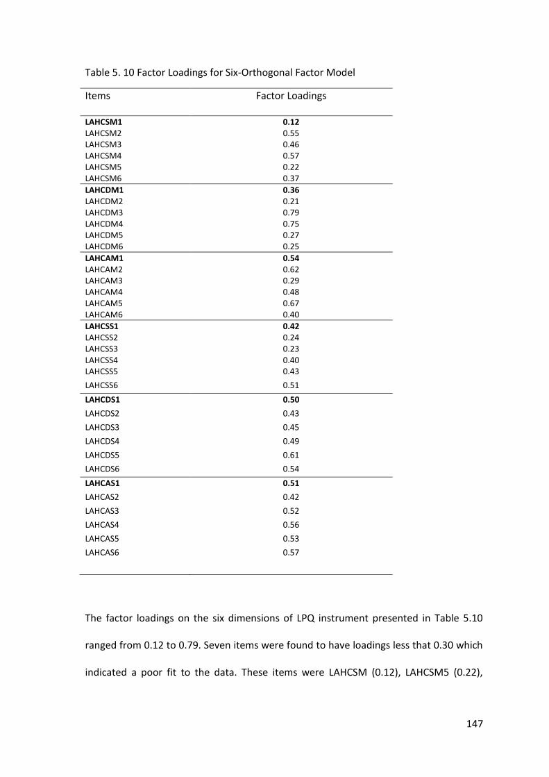
147

Table 5. 10 Factor Loadings for Six-Orthogonal Factor Model

Items Factor Loadings

LAHCSM1 0.12 LAHCSM2 0.55 LAHCSM3 0.46 LAHCSM4 0.57 LAHCSM5 0.22 LAHCSM6 0.37

LAHCDM1 0.36 LAHCDM2 0.21 LAHCDM3 0.79 LAHCDM4 0.75 LAHCDM5 0.27 LAHCDM6 0.25

LAHCAM1 0.54 LAHCAM2 0.62 LAHCAM3 0.29 LAHCAM4 0.48 LAHCAM5 0.67 LAHCAM6 0.40

LAHCSS1 0.42 LAHCSS2 0.24 LAHCSS3 0.23 LAHCSS4 0.40 LAHCSS5 0.43

LAHCSS6 0.51

LAHCDS1 0.50

LAHCDS2 0.43

LAHCDS3 0.45

LAHCDS4 0.49

LAHCDS5 0.61

LAHCDS6 0.54

LAHCAS1 0.51

LAHCAS2 0.42

LAHCAS3 0.52

LAHCAS4 0.56

LAHCAS5 0.53

LAHCAS6 0.57

The factor loadings on the six dimensions of LPQ instrument presented in Table 5.10

ranged from 0.12 to 0.79. Seven items were found to have loadings less that 0.30 which

indicated a poor fit to the data. These items were LAHCSM (0.12), LAHCSM5 (0.22),

148

LAHCDM2 (0.21), LAHCDM5 (0.27), LAHCDM6 (0.25), LAHCAM3 (0.29), LAHCSS2 (0.24)

and LAHCSS3 (0.23). However, the rest of the items showed moderate factor loadings.

Table 5. 11 Fit Indices for the Six- Orthogonal Factor Models

INDICES Six-Factor

LACH/LPQ


Degree of Freedom

594 11.2


0.41


0.48

Root Mean Square Error of Approximation (RMSEA) 0.08

Diamantoplous and Siguaw (2000) claimed that a value of RMSEA less than 0.05 is

accepted as indicating a good fit, values between 0.05 and under 0.08 a reasonable fit,

values between 0.08 and under 0.10 a mediocre fit and values under 0.10 a poor fit.

Based on this claim, it was found that this model demonstrated a mediocre fit to the

sample data because the RMSEA values of the Six-Factor Model was 0.08. Moreover,

the TLI and CLI for both models were less than 0.90. These results indicate that the

model had room for improvement. Consequently, further testing was carried out using

alternative models. The results are reported in the following section.

Confirmatory Factor Analysis of the Alternative Model

Four alternative models were tested and compared, to identify which would adequately

fit the sample data. The four models were (a) Six-Factor Correlated Model, (b) Six Factor

Hierarchical Order Model (c) Six Factor Hierarchical Second Model and, (d) Six Factor

Hierarchical Third Order Model (see Figure 5.5). Furthermore, CFA was carried out to

confirm whether the observed variables were measuring the latent variables which they

149

were represented to measure in the instrument. The variables are presented in Figure

5.5, followed by the factor loadings of the LAHC in Table 5.12 and the model fit indices

in Table 5.13.

Table 5. 12 Factor loadings of items in Six-Factor Correlated Model, Hierarchical Model Second Order and Hierarchical Model Third Order

Variables Subscale Six-Factor Correlated Model

Hierarchical Model

Variables Scale Subscale Hierarchical Second Order Model

Hierarchical Third Order Model

LAHCSM1 Surface 0.11 0.04 LAHCSM1 Surface 0.33 0.11 LAHCSM2 Motive 0.45 0.48 LAHCSM2 Motive 0.48 0.44 LAHCSM3 0.57 0.58 LAHCSM3 0.54 0.55 LAHCSM4 0.48 0.52 LAHCSM4 0.52 0.48 LAHCSM5 0.24 0.18 LAHCSM5 0.26 0.27 LAHCSM6 0.43 0.39 LAHCSM6 Surface 0.45 0.45

LAHCDM1 Deep 0.43 0.44 LAHCSS1 Surface 0.29 0.42 LAHCDM2 Motive 0.28 0.28 LAHCSS2 Strategy 0.50 0.27 LAHCDM3 0.70 0.69 LAHCSS3 0.48 0.25 LAHCDM4 0.70 0.69 LAHCSS4 0.14 0.37 LAHCDM5 0.35 0.35 LAHCSS5 0.38 0.43 LAHCDM6 0.37 0.38 LAHCSS6 0.28 0.50

LAHCAM1 Achieving 0.52 0.50 LAHCDM1 Deep 0.45 0.44 LAHCAM2 Motive 0.68 0.70 LAHCDM2 Motive 0.26 0.26 LAHCAM3 0.26 0.28 LAHCDM3 0.70 0.70 LAHCAM4 0.48 0.47 LAHCDM4 0.71 0.72 LAHCAM5 0.63 0.63 LAHCDM5 0.34 0.34 LAHCAM6 0.39 0.38 LAHCDM6 Deep 0.36 0.35

LAHCSS1 Surface 0.47 0.44 LAHCDS1 Deep 0.45 0.46 LAHCSS2 Strategy 0.23 0.21 LAHCDS2 Strategy 0.47 0.47 LAHCSS3 0.19 0.20 LAHCDS3 0.50 0.50 LAHCSS4 0.37 0.41 LAHCDS4 0.46 0.46 LAHCSS5 0.41 0.41 LAHCDS5 0.63 0.63 LAHCSS6 0.53 0.52 LAHCDS6 0.49 0.49

LAHCDS1 Deep 0.46 0.47 LAHCAM1 Achieving 0.50 0.51 LAHCDS2 Strategy 0.45 0.47 LAHCAM2 Motive 0.69 0.69 LAHCDS3 0.49 0.52 LAHCAM3 0.28 0.27 LAHCDS4 0.47 0.46 LAHCAM4 0.48 0.47 LAHCDS5 0.64 0.61 LAHCAM5 0.62 0.63 LAHCDS6 0.50 0.49 LAHCAM6 Achieving 0.39 0.39

LAHCAS1 Achieving 0.50 0.50 LAHCAS1 Achieving 0.51 0.49 LAHCAS2 Strategy 0.45 0.45 LAHCAS2 Strategy 0.45 0.46 LAHCAS3 0.49 0.49 LAHCAS3 0.49 0.49 LAHCAS4 0.53 0.52 LAHCAS4 0.53 0.51 LAHCAS5 0.55 0.56 LAHCAS5 0.55 0.56 LAHCAS6 0.59 0.59 LAHCAS6 0.59 0.59

150

Figure 5. 5 (a) Six Factor Correlated (b) Six Factor Hierarchical (c) Six Factor Hierarchical Second Order d) Six Factor Hierarchical Third Order Models of LAC

Surface Motive

.01

LAHCSM1e1

.11.20

LAHCSM2e2

.45.32

LAHCSM3e3.57

.23

LAHCSM4e4 .48

.06

LAHCSM5e5 .24

.19

LAHCSM6e6.43

DeepMotive

.19

LAHCDM1e7

.08

LAHCDM2e8

.49

LAHCDM3e9

.49

LAHCDM4e10

.12

LAHCDM5e11

.14

LAHCDM6e12

.43

.28

.70.70.35.37

AchievingMotive

.27

LAHCAM1e13

.47

LAHCAM2e14

.07

LAHCAM3e15

.23

LAHCAM4e16

.40

LAHCAM5e17

.15

LAHCAM6e18

.52

.68

.26.48.63.39

SurfaceStrategy

.22

LAHCSS1e19

.05

LAHCSS2e20

.04

LAHCSS3e21

.14

LAHCSS4e22

.17

LAHCSS5e23

.28

LAHCSS6e24

.47

.23

.19.37.41.53

DeepStrategy

.21

LAHCDS1e25

.21

LAHCDS2e26

.24

LAHCDS3e27

.22

LAHCDS4e28

.40

LAHCDS5e29

.25

LAHCDS6e30

.46

.45

.49.47.64.50

AchievingStrategy

.25

LAHCAS1e31

.20

LAHCAS2e32

.24

LAHCAS3e33

.28

LAHCAS4e34

.30

LAHCAS5e35

.35

LAHCAS6e36

.50

.45

.49.53.55.59

.46

.74

.40

.34

.46

.82

-.11

.91

.74

.07

.73

.71-.10

-.13

.95

.30

Surface Motive

.00

LAHCSM1 e1.04 .23

LAHCSM2 e2.48.33

LAHCSM3 e3.58

.27

LAHCSM4 e4

.52

.03

LAHCSM5 e5

.18

.15

LAHCSM6 e6

.39

.85

DeepMotive

.20

LAHCDM1 e7.08

LAHCDM2 e8.48

LAHCDM3 e9.48

LAHCDM4 e10.13

LAHCDM5 e11.14

LAHCDM6 e12

.44.28.69

.69

.35

.38

.71

AchievingMotive

.25

LAHCAM1 e13.48

LAHCAM2 e14.08

LAHCAM3 e15.23

LAHCAM4 e16.39

LAHCAM5 e17.15

LAHCAM6 e18

.50.70.28

.47

.63

.38

.00

SurfaceStrategy

.19

LAHCSS1 e19.04

LAHCSS2 e20.04

LAHCSS3 e21.17

LAHCSS4 e22.17

LAHCSS5 e23.27

LAHCSS6 e24

.44.21.20

.41

.41

.52

.94

DeepStrategy

.22

LAHCDS1 e25.22

LAHCDS2 e26.27

LAHCDS3 e27.21

LAHCDS4 e28.38

LAHCDS5 e29.24

LAHCDS6 e30

.47.47.52

.46

.61

.49

.79

AchievingStrategy

.25

LAHCAS1 e31.20

LAHCAS2 e32.24

LAHCAS3 e33.27

LAHCAS4 e34.31

LAHCAS5 e35.35

LAHCAS6 e36

.50.45.49

.52

.56

.59

LearningApproaches

HistoryClassroom

.55

.92

.84

-.06

.97

.89

e37

e38

e39

e40

e41

e42

6.94

Surface Motive

.01

LAHCSM1 e1.11 .19

LAHCSM2 e2.44 .30

LAHCSM3 e3.55.23

LAHCSM4 e4.48

.07

LAHCSM5 e5

.27

.20

LAHCSM6 e6

.45

.83

DeepMotive

.19

LAHCDM1 e7.07

LAHCDM2 e8.49

LAHCDM3 e9.51

LAHCDM4 e10.12

LAHCDM5 e11.13

LAHCDM6 e12

.44.26.70

.72

.34

.35

.72

AchievingMotive

.26

LAHCAM1 e13.48

LAHCAM2 e14.07

LAHCAM3 e15.22

LAHCAM4 e16.39

LAHCAM5 e17.15

LAHCAM6 e18

.51.69.27

.47

.63

.39

.03

SurfaceStrategy

.18

LAHCSS1 e19.07

LAHCSS2 e20.06

LAHCSS3 e21.14

LAHCSS4 e22.19

LAHCSS5 e23.25

LAHCSS6 e24

.42.27.25

.37

.43

.50

.99

DeepStrategy

.21

LAHCDS1 e25.22

LAHCDS2 e26.25

LAHCDS3 e27.21

LAHCDS4 e28.40

LAHCDS5 e29.24

LAHCDS6 e30

.46.47.50

.46

.63

.49

.72

AchievingStrategy

.24

LAHCAS1 e31.21

LAHCAS2 e32.24

LAHCAS3 e33.26

LAHCAS4 e34.31

LAHCAS5 e35.35

LAHCAS6 e36

.49

.46.49

.51

.56

.59

.04

Surface

.58

Deep

1.71

Achieving

LACH

2.63

.85

.91

.99

.17

.85

e37

e38

e39

e40

e41

e42

e43

e44

e45

1.31

.76

.21

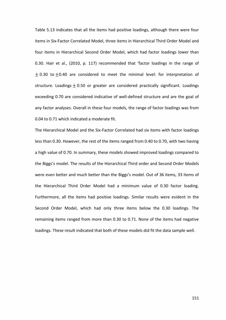
151

Table 5.13 indicates that all the items had positive loadings, although there were four

items in Six-Factor Correlated Model, three items in Hierarchical Third Order Model and

four items in Hierarchical Second Order Model, which had factor loadings lower than

0.30. Hair et al., (2010, p. 117) recommended that ‘factor loadings in the range of

0.30 to 0.40 are considered to meet the minimal level: for interpretation of

structure. Loadings 0.50 or greater are considered practically significant. Loadings

exceeding 0.70 are considered indicative of well-defined structure and are the goal of

any factor analyses. Overall in these four models, the range of factor loadings was from

0.04 to 0.71 which indicated a moderate fit.

The Hierarchical Model and the Six-Factor Correlated had six items with factor loadings

less than 0.30. However, the rest of the items ranged from 0.40 to 0.70, with two having

a high value of 0.70. In summary, these models showed improved loadings compared to

the Biggs’s model. The results of the Hierarchical Third order and Second Order Models

were even better and much better than the Biggs’s model. Out of 36 items, 33 items of

the Hierarchical Third Order Model had a minimum value of 0.30 factor loading.

Furthermore, all the items had positive loadings. Similar results were evident in the

Second Order Model, which had only three items below the 0.30 loadings. The

remaining items ranged from more than 0.30 to 0.71. None of the items had negative

loadings. These result indicated that both of these models did fit the data sample well.

152

Table 5. 13 Fit Indices for the Six-Factor Models

INDICES Six-Factor Correlated

Hierarchical Model

Hierarchical Second Order

Hierarchical Third Order


3986.35

3949.91 3774.282

Degree of Freedom

(579) 6.17

(588) 6.78

(589) 6.71

(585) 6.45


0.66

0.67

0.68


0.74 0.70 0.71 0.72


0.06 0.06 0.06

0.06

The fit indices based on the AMOS program (Arbuckle, 1999) for the last four alternative

models are presented in Table 5.14. The value of chi-square divided by the degree of

freedom (

) of the alternative models ranged from 6.17 - 6.71. This result indicated

that the models were close to the critical value of 5. The RMSEA is another indicator

used to describe the model fit. The RMSEA value shows ‘how well would the model,

with unknown but optimally chosen parameter values, fit the population covariance

matrix if it were available’ (Diamantoplous & Siguaw, 2000, p. 85). The RMSEA values of

all four models showed an identical result (0.06), which indicated that the models had a

reasonable fit. On the order hand, the values of TLI and CFI values were less than 0.90,

which indicated a moderate fit to the models. As a consequence of these results, the Six

Factor Hierarchical Second Order Model was used for the PLSPATH analysis.

153

5.6 The Students’ Perception of History Questionnaire (SPERCH)

This instrument of 10 items was designed to measure the students’ perceptions of

History learning objectives in the classroom. This instrument was developed by the

researcher, and was grounded on the History Learning Objectives stated in the

Malaysian History syllabus (Ministry of Education, Malaysia, 2002). There were three

subscales in the instrument namely country, community and individual. Each item

response used a five-point Likert scale: 1. Strongly Disagree 2. Disagree 3. No opinion 4.

Agree 5. Strongly Agree. The internal consistency value for this instrument was 0.88.


An Exploratory Factor Analysis (EFA) was carried out to examine the factorial structure

of this newly developed instrument. In addition, Confirmatory Factor Analysis (CFA) was

performed to validate the SPERCH instrument. According to Curtis (2005, p. 183), EFA is

used to show that ‘the patterns of response to the items of the instrument reflect the

constructs that were used in framing the instrument’. In this study, EFA was employed

using principal components extraction, followed by varimax rotation, using SPSS version

17.

154

Table 5. 14 Rotated factor solution for an exploratory analysis of the SPERCH (New Structure)

Item no. Sub-scale Factor 1 Factor 2 Factor 3 SPERCH1 Country 0.69 SPERCH2 0.78 SPERCH3 0.68 SPERCH4 0.54 SPERCH5 Community 0.72 SPERCH6 0.79 SPERCH7 0.65 SPERCH8 Individual 0.70

SPERCH9 0.82

SPERCH10 0.62

Factor loadings for the SPERCH instruments are presented in Table 5.15. The factor

loadings range from 0.54 to 0.79 which indicates that the items the best indicators for

these factors. Therefore, no items were removed from the instruments. Although EFA

showed that most of the items reflected the construct and showed coverage of the

items, according to Curtis (2005, p. 185) EFA fails to show whether the constructs form a

certain concept. Due to these limitations, CFA was carried further in this study, to

determine the structure of the constructs and to test the model fit. As alternatives

models, four models were tested namely; (a) One Factor Model (b) Three Factor

Orthogonal Model (c) Three factor Correlated Model and (d) Three Factor Hierarchical

Model.

Confirmatory Factor Analysis for the Alternative Model

As a first step, the One-Factor Model was tested in CFA to determine the model fit. CFA

examines how well the observed variables reflect the latent variables which they are

represented to measure in the instrument. This model consisted of 10 items. Model fit

and factor loadings are discussed in this analysis. The results are presented in Table 5.16.

155

SPERCH

.42

SPERCH1 e1

.65

.43

SPERCH2 e2

.66

.52

SPERCH3 e3

.72.40

SPERCH4 e4

.63 .47

SPERCH5 e5.68

.45

SPERCH6 e6

.67

.54

SPERCH7 e7

.74

.46

SPERCH8 e8

.68

.39

SPERCH9 e9

.62

.44

SPERCH10 e10

.67

The factor structure is presented in Figure 5.7. Most of the loadings have been above

0.50, which indicated that the items were strongly correlated. Overall, the items had

strong factor loadings onto the latent factors. However it was considered necessary to

test alternative models such as, Three-Factor Correlated and Three-Factor Hierarchical

Models in further analysis.

Figure 5. 6 One - Factor Model

Table 5. 15 Factor loadings of the SPERCH

Item no. Factor Loadings

SPERCH1 0.65 SPERCH2 0.66 SPERCH3 0.72 SPERCH4 0.63 SPERCH5 0.68 SPERCH6 0.67 SPERCH7 0.74 SPERCH8 0.68 SPERCH9 0.62 SPERCH10 0.67

156

Table 5. 16 Fit Indices for the One-Factor Model

INDICES One-Factor

Model SPERCH

Chi –Square

543.94

Degree of Freedom

35 15.54

Tucker-Lewis Index (TLI) 0.88 Comparative Fit Index (CFI) 0.92 Root Mean Square Error of Approximation (RMSEA) 0.09

The fit indices for the One-Factor Initial Model are presented in Table 5.16. The values

of TLI (0.88) and CFI (0.92) were reasonable. Furthermore, the RMSEA value of 0.09

indicated that the model had a mediocre fit. Based on the fit indices given in Table 5.16

this model can be improved. Therefore, further analysis was carried out with the

alternative models to identify which alternative structures had the best fit indices.

The three alternative models were tested using AMOS (Version 17) namely; (a) Three

Factor Orthogonal Model, (b) Three Factor Correlated Model and, (c) Three Factor

Hierarchical Model (see Figure 5.7). Based on EFA there were three subscales in SPERCH,

namely a) country, b) community, and c) individual. The instrument consisted of 10

items. The Country subscale had 3 items, the Community subscale had 4 items and the

Individual subscale had 3 items. The results of the CFA procedure are displayed in terms

of factor loadings (see Table 5.17) and fit indices (see Table 5.18). AMOS was used to

carry out CFA and to draw the diagram, presented in Figure 5.7.

157

Figure 5. 7 (a) One Factor (b) Three Factor Orthogonal (c) Three Factor Correlated (d) Three Factor Hierarchical Models of SPER

158

Table 5. 17 Factor Loading of the Alternative Models

Item no. Sub-scale Three-Factor Orthogonal SPERCH

Three-Factor Correlated SPERCH

Three-Factor Hierarchical SPERCH

SPERCH5 Country 0.72 0.72 0.72 SPERCH6 0.74 0.72 0.72 SPERCH7 0.76 0.78 0.78

SPERCH1 Community 0.64 0.68 0.68 SPERCH2 0.71 0.71 0.71 SPERCH3 0.79 0.77 0.77 SPERCH4 0.65 0.66 0.66

SPERCH8 Individual 0.73 0.72 0.72 SPERCH9 0.75 0.69 0.69 SPERCH10 0.65 0.70 0.70

The factor loadings for the Alternative Models which are presented in Table 5.17 ranged

from 0.65 to 0.79. Factor loadings for Three Factor Hierarchical Model showed the same

values as the Three-Factor Correlated Model, while the Three Factor Orthogonal Model

showed only slight differences in factor loadings. In relation to fit indices, the Three

Factor Hierarchical Model showed a better fit compared to the other models. The fit

indices of these models are presented in Table 5.18.

Table 5. 18 Fit Indices for the Alternative Models

INDICES Three-Factor Orthogonal SPERCH

Three-Factor Correlated SPERCH

Three-Factor Hierarchical SPERCH

Chi –Square

2332.47 258.97 262.47

Degree of Freedom

35 66.6

32 8.09

34 7.72


0.94

0.94


0.65 0.97 0.97


0.19 0.07 0.06

159

The value of chi-square divided by the degree of freedom (

) of the alternative models

was well over 5, which indicates a poor fit to the data. However, the values of the

RMSEA index for the Three-Factor correlated (0.07) and Hierarchical Models (0.06)

showed a reasonable level of fit. In addition, TLI and CFI showed values above than 0.90

for both models. These values indicated that both models did fit the sample data. Based

on the RMSEA values, it was concluded that the Hierarchical Model was the best fit for

the sample data and consequently used for the subsequent analysis.

5.8 Summary

The students’ instruments comprised three questionnaires: (a) the classroom climate

(ICEQ),

(b) the students’ learning process (LPQ), and (c) the perception towards learning History

(SPERCH). The validation was based on the sample data of 1653 students.

Each instrument underwent the same process of validation, using Confirmatory Factor

Analysis (CFA) and Exploratory Factor Analysis (EFA) as required. Two sets of models

were discussed in detail for all questionnaires, the Baseline Confirmatory and

Alternative Models. The CFA and EFA were discussed in terms of the factor loadings and

model fit indices. All instruments were tested for the model fit to the sample data.

Finally, the alternative model which had the best fit was selected for further analyses.

Across the three instruments, the models used in this study were as follows.

1. The Individualised Classroom Environment Questionnaire (ICEQ) was developed

by Barry Fraser’s (1990). ICEQ measured the effect of the classroom environment

160

of History students. For this instrument, the Five Factor Hierarchical (for both CCA

and CCP) was chosen for the further analysis.

2. The Learning Process Questionnaires (LPQ) was developed by Biggs (1987) to

measure students’ learning approaches. From the results of the CFA, the Six

Factor Hierarchical Second Order Models was chosen for further analysis.

3. The Students’ Perception of History Questionnaire (SPERCH) was developed by the

researcher and was based on the History Learning Objectives in the Malaysian

History syllabus (Ministry of Education, Malaysia, 2002). This instrument was

developed to explore the students’ perceptions of the learning outcomes in the

History classroom. As a result of the CFA, the Hierarchical Model was selected for

further analysis.

The following chapter reports and discusses the findings concerning the relationships

among teachers’ variables using Partial Least Square Path Analysis (PLSPATH).

161

Chapter 6 Respondents’ Demographic

Information and Out-of-field and In-field Teachers Differences __________________________________________________________

6.1 Introduction

Respondents’ Demographics

In the first part of this chapter, the demographic information of the 1653 student and

52 teacher respondents from 18 public schools in Kuala Lumpur are described. The SPSS

program was used to analyse the descriptive data on gender, age, ethnic groups,

education, as well as occupation and the results are presented in this chapter. The

second part of the chapter considers the comparison between the out-of-field and in-

field teachers using the t-test procedure on a range of variables. These include, teaching

experience, teaching conceptions, teaching methods, teaching approaches, as well as

students’ classroom climate, preferred and actual, students’ learning approaches and

students’ learning outcomes in History. The scale scores for each of the constructs

discussed were calculated using AMOS factor score weights. The results presented in

this chapter are important as they provide the necessary preparation for subsequent

analyses.

162

6.2 Teachers’ Demographics

Gender and Age

Table 6.1, as well as Figures 6.1 and 6.2, depict the teachers’ distribution according to

their gender and age. Of the 52 teachers, 37 (71.2%) were females and 15 (28.8%) were

males. The largest group of teachers were those between the age of 31 and 40 years old

(40%). The second and third largest groups in this study were in the age group 21-30

years (25%) and the age group 41-50 years (21. %) respectively. In total, 87% of

respondents were in the age group range 21-50 years.

Table 6. 1 Gender and Age of the Teacher Respondents

Frequency Percentage

Gender Male 15 28.8 Female 37 71.2 Total 52 100 Age (years) Below 20 0 0 21-30 13 25.0 31-40 21 40.3 41-50 11 21.2 Above 50 7 13.5

Total 52 100.0

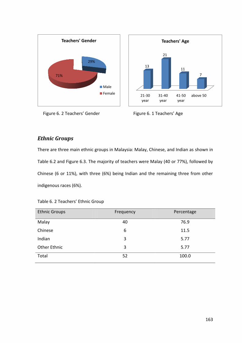
163

29%

71%

Teachers' Gender

Male

Female21-30year

31-40year

41-50year

above 50

13

21

11

7

Teachers' Age

Figure 6. 1 Teachers’ Age Figure 6. 2 Teachers’ Gender

Ethnic Groups

There are three main ethnic groups in Malaysia: Malay, Chinese, and Indian as shown in

Table 6.2 and Figure 6.3. The majority of teachers were Malay (40 or 77%), followed by

Chinese (6 or 11%), with three (6%) being Indian and the remaining three from other

indigenous races (6%).

Table 6. 2 Teachers’ Ethnic Group

Ethnic Groups Frequency Percentage

Malay 40 76.9

Chinese 6 11.5

Indian 3 5.77

Other Ethnic 3 5.77

Total 52 100.0

164

Figure 6. 3 Teachers’ Ethnic Group

Level of Education

All the teachers (52) involved in this research held bachelor degrees and were graduates

from various universities in Malaysia. Of the 52 teachers, 16 (30.7%) also held a

diplomas in either education, early education, investment analysis, or management.

Besides that, there were four (7.69%) teachers who had a master’s degree in education

(see Table 6.3 and Figure 6.4). In summary, there were 26 out-of-field teachers and 26

in-field History teachers, with the difference between them being that the qualifications

of the out-of-field teachers did not include any specialisation in History.

77%

11%

6% 6%

Teachers' Ethnic Group

Malay

Chinese

Indian

Others EthnicGroups

165

Table 6. 3 Teacher Respondents’ Distribution According to their Qualification Level

Qualification Level Frequency Percentage

Master & Bachelor Degree 4 7.69

Diploma & Bachelor Degree 16 30.7

Bachelor Degree 32 61.5

Total 52 100.0

Figure 6. 4 Teacher Respondents’ Qualification Level

Work experience

The retirement age of government servants in Malaysia is 60 years, according to

government policy. The retirement age applies to everybody regardless of their

qualification or position in the school (Public Service of Department of Malaysia, 2008).

Most of the teachers in this research had taught between 2-5 years, (29%). A small

number of respondents had served between 21-25 years (5%). Only five (9%) teachers

8%

30%

62%

Teachers' Qualification Level

Master & BachelorDegreeDiploma & BachelorDegreeBachelor Degree

166

had worked for more than 25 years. Moreover, 20% of the teachers had worked

between 6-10 years, 17% for 11-51 years, 13% for 16-20 years, and 6% for 0-1year (see

Table 6.4 and Figure 6.5).

Table 6. 4 Teacher Respondents’ Distribution According to Work Experience

Work Experience (years) Frequency Percentage

0-1 3 5.7

2-5 15 29.0

6-10 11 21.2

11-15 9 17.3

16-20 6 11.5

21-25 3 5.7

> 25 5 9.6

Total 52 100.0

Figure 6. 5 Teachers’ Work Experiences

0-1 year

2-5 year

6-10 year

11-15 year

16-20 year

21-25 year

above 25 year

3

15

11

9

6

3

5

Respondents' Work Experience

167

6.3 Students’ Demographics

Gender and Age

From the total of 1653 student respondents, 963 (58.3%) were female and 689 (41.7%)

were male. The gender and age breakdown are shown in the table and figures below.

There were two age groups in this study. As mentioned in Chapter 1, the respondents

were Form Four students, with an average age of 16 years old. However, there were a

few who were 17 years old at the time of the study. This is because these students came

from Chinese school where they had joined the secondary school a year later than the

students selected from the government schools. The largest group of students were 16

years of age (95%), followed by those who were 17 years of age (4%). The data with

regard to the students’ age are given in Table 6.5 and Figures 6.6 and 6.7 below.

Table 6. 5 Gender and Age of Student Respondents

Frequency Percentage

Gender Male 689 41.7 Female 964 58.3

Total 1653 100

Age (years) 16 1580 95.6 17 73 4.4

Total 1653 100

42%

58%

Students' Gender

Male

Female

16 year 17 year

1580

73

Students' Age

Figure 6. 6 Students’ Age Figure 6. 7 Students’ Gender

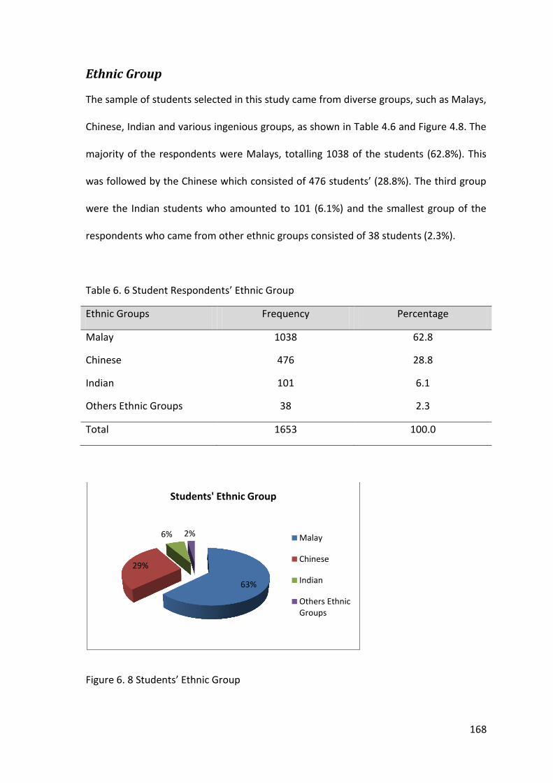
168

Ethnic Group

The sample of students selected in this study came from diverse groups, such as Malays,

Chinese, Indian and various ingenious groups, as shown in Table 4.6 and Figure 4.8. The

majority of the respondents were Malays, totalling 1038 of the students (62.8%). This

was followed by the Chinese which consisted of 476 students’ (28.8%). The third group

were the Indian students who amounted to 101 (6.1%) and the smallest group of the

respondents who came from other ethnic groups consisted of 38 students (2.3%).

Table 6. 6 Student Respondents’ Ethnic Group

Ethnic Groups Frequency Percentage

Malay 1038 62.8

Chinese 476 28.8

Indian 101 6.1

Others Ethnic Groups 38 2.3

Total 1653 100.0

Figure 6. 8 Students’ Ethnic Group

63%

29%

6% 2%

Students' Ethnic Group

Malay

Chinese

Indian

Others EthnicGroups

169

Mother’s Education Level

In terms of education level, about 60% of the students’ mothers had completed their

primary and high school education and 27% of the respondents’ mothers had at least a

tertiary education background (Diploma or university degree) as presented in Table 6.7

and Figure 6.9.

Table 6. 7 Mothers’ Education Level

Education level Frequency Percentage

No formal education 24 1.5 Primary education 127 7.7 Secondary education 926 56.0 Diploma 255 15.4 Degrees 146 8.8 Post graduate 57 3.4

Sub total 1535 92.9 No Answer 118 7.1

Total 1653 100.0

Figure 6. 9 Mothers’ Education Level

Father’s Education Level

Table 6.8 and Figure 6.10 present the students’ fathers’ education background. It shows

that 54.3% of the respondents’ fathers had a tertiary diploma or a university degree,

with 34% having only primary and high school background.

2% 8%

56%

15%

9% 3% 7%

Mothers' Education Level

No formal educationPrimary educationSecondary educationDiplomaDegreesPost graduate

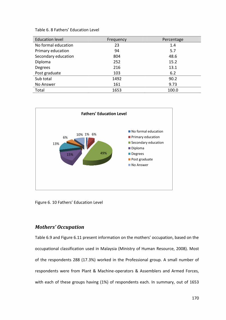
170

Table 6. 8 Fathers’ Education Level

Education level Frequency Percentage

No formal education 23 1.4 Primary education 94 5.7 Secondary education 804 48.6 Diploma 252 15.2 Degrees 216 13.1 Post graduate 103 6.2

Sub total 1492 90.2 No Answer 161 9.73

Total 1653 100.0

Figure 6. 10 Fathers’ Education Level

Mothers’ Occupation

Table 6.9 and Figure 6.11 present information on the mothers’ occupation, based on the

occupational classification used in Malaysia (Ministry of Human Resource, 2008). Most

of the respondents 288 (17.3%) worked in the Professional group. A small number of

respondents were from Plant & Machine-operators & Assemblers and Armed Forces,

with each of these groups having (1%) of respondents each. In summary, out of 1653

1% 6%

49% 15%

13%

6% 10%

Fathers' Education Level

No formal education

Primary education

Secondary education

Diploma

Degrees

Post graduate

No Answer

171

under two fifths or 632 (38.5%) of the mothers were working, while, the remaining 1016

(61.5%) were not.

Table 6. 9 Respondents Mothers’ Occupation

Occupational Classification Frequency Percentage

Managers 88 5.3 Professionals 286 17.3 Technicians & Associate Professionals 37 2.2 Clerical Support Workers 118 7.1 Service & Sales Workers 76 4.6 Craft & Related Trades Workers 6 0.4 Plant & Machine-operators & Assemblers

2 0.1

Elementary occupations 22 1.3 Armed Forces Occupations 2 0.1 Total 637 38.5 No Job 1016 61.5

Total 1653 100.0

Figure 6. 11 Mothers’ Occupations (Students)

88

286

37 118 76 6 2 22 2

1016

Mothers' Occupations (Students)

172

Fathers’ Occupation

Table 6.10, and Figure 6.12 show that more than three quarters of the respondents’

fathers (1293 or 78.2%) worked in one of the 10 sectors (Ministry of Human Resource

2008). Most of the fathers, 392 (23.7%) worked in the Service and Sales sectors. The

second largest group was Professional (289 or 17.5%), with only one person (1%)

working in the Skilled Agricultural, Forestry and Fishery sector. There were 360 fathers

(21.85%) who were unemployed.

Table 6. 10 Fathers’ Occupation

Occupational Classification Frequency Percentage

Managers 128 7.7 Professionals 289 17.5 Technicians & Associate Professionals 92 5.6 Clerical Support Workers 79 4.8 Service & Sales Workers 392 23.7 Skilled Agricultural, Forestry & Fishery Workers

1 0.1

Craft & Related Trades Workers 97 5.9 Plant & Machine-operators & Assemblers 131 7.9 Elementary Occupations 48 2.9 Armed Forces Occupations 36 2.2

Sub total 1293 78.2 No Jobs 360 21.8

Total 1653 100.0

Figure 6. 12 Fathers’ Occupations (Students)

128

289

92 79

392

1 97 131

48 36

360

Fathers' Occupation (Students)

173

6.4 Comparisons of out-of field and in-field History teacher: Teachers’ and Students’ characteristics

This study was focused on two groups of teachers, out-of-field and in-field History

teachers in Malaysian secondary schools. The two independent samples t-test was used

to compare out-of-field and in-field History teachers on a range of teacher

characteristics (teaching experience, teaching conceptions, teaching approaches and

teaching method) and the characteristics of students they taught (classroom climate

actual, classroom climate preferred, students’ learning approaches and History learning

outcomes).

Teachers’ Characteristics

Years of teaching (TExperience)

Table 6. 11 Descriptive statistics for teacher experience

Type of teachers N Mean

Std. Deviation

Std. Error Mean

Sig. (2-tailed)

Mean Difference

TYRTEAC out-of-field 26 7.4704 8.00605 1.54076 .002 -7.49117

in-field 26 14.9615 8.39276 1.64596

174

Figure 6. 13 Years of teaching (Teacher experience) reported by in-field and out-of-field teachers

To investigate the difference in experience between the out-of-field (OFT) teachers and

the in-field (IF) History teachers, the independent sample t-test was carried out. The

results showed that there was a significant (p = 0.002) difference in the average number

of years teaching between the two groups of History teachers (see Table 6.11 and

Figure 6.13). Out-of-field teachers had an average of seven and a half years of

experience compared to in-field teachers who had more than 14 years’ experience of

teaching. This indicates that in-field teachers are more experienced in teaching History

compared to the out-of-field teachers, as the two error-bar plots in Figure 4.1

demonstrate the mean, within the 95% confidence intervals of the teacher experience.

Teacher Qualification

175

Teaching Conceptions (TCont)

Table 6. 12 Descriptive statistics for teacher conceptions


Std. Deviation

Std. Error Mean

Sig. (2-

tailed)

Mean Difference

TAbilityDev out-of-field 26 -.1135 .89452 .17215 .270 -.29987

in-field 26 .1864 1.05887 .20766

TAttPro out-of-field 26 -.1282 .78391 .15086 .220 -.32502

in-field 26 .1968 1.10134 .21599

TKnowDeli out-of-field 26 -.0271 .86917 .16727 .766 -.08231

in-field 26 .0552 1.11981 .21961

TExamPrep out-of-field 26 .0152 .85520 .16458 .887 -.03928

in-field 26 .0545 1.12589 .22081

TConDance out-of-field 26 -.2549 .97406 .18746 .031 -.57593

in-field 26 .3210 .91090 .17864

Figure 6. 14 Teaching conceptions reported by in-field and out-of-field teachers

In terms of teaching conceptions, there were five dimensions used to reflect the latent

variable ‘Teaching Conceptions (TCont)’, namely: AbilityDev, AttPro, KnowDeli,


176

ExamPrep and ConDance. Table 4.12 shows the comparison between the in-field (IF)

and the out-of-field (OFT) History teachers for the five dimensions. The results of

independent sample t-test showed that there were no significant differences between

the two groups for four out of five dimensions tested. A significant difference was found

only for the dimension of conduct guidance (ConDance). This dimension measured the

teachers’ influence as role model and nurturer of good conduct in the classroom. The

results showed that in-field teachers had a higher level of conception than the out-of-

field teachers with respect to presenting good role models and guiding students toward

good conduct.

Teaching Approaches (TApp)

Table 6. 13 Descriptive statistics for teaching approaches


Std. Deviation

Std. Error Mean

Sig. (2-tailed)

Mean Difference

TInfoTrans out-of-field 26 2.4426 .40905 .07872 .909 .01390

in-field 26 2.4287 .47253 .09267

TConChan out-of-field 26 2.8470 .42877 .08252 .449 -.08369

in-field 26 2.9307 .36541 .07166

177

Figure 6. 15 Teaching approaches reported by in-field and out-of-field teachers

Two scales were used to measure the constructs of teaching approaches (TApp), namely:

conceptual change or student or focused (CCSF) and information transmission or

teacher-focused (ITTF) scale, labelled as TConChan and TInfoTrans respectively. The

comparison between in-field (IF) and out-of-field (OFT) History teachers in relation to

their teaching approaches are presented in Table 6.13 and Figure 6.15. Even though the

differences were not significant for any scales, the patterns are worth being considered.

In general, in-field teachers focused more on conceptual change and less on the

information transfer compared to out-of-field teachers.


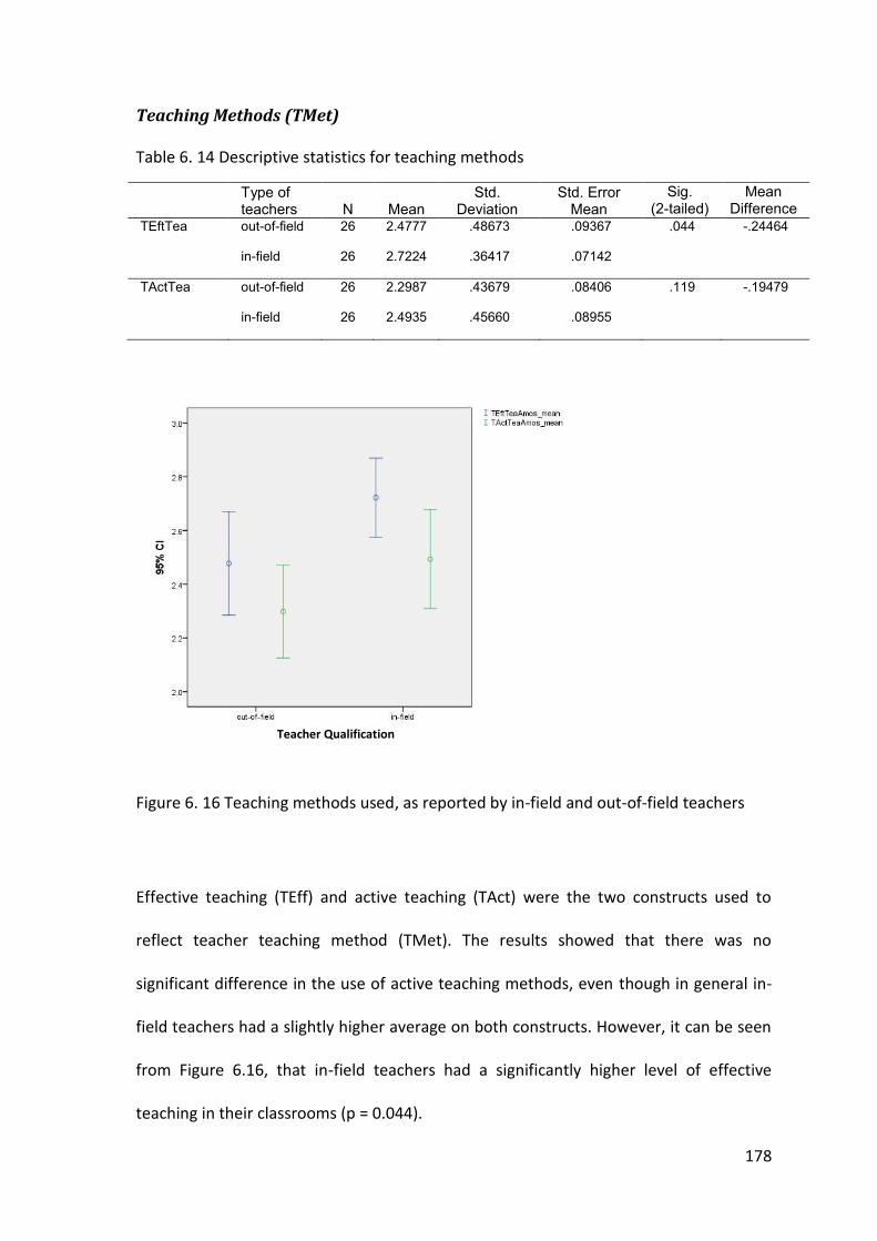
178

Teaching Methods (TMet)

Table 6. 14 Descriptive statistics for teaching methods


Std. Deviation

Std. Error Mean

Sig. (2-tailed)

Mean Difference

TEftTea out-of-field 26 2.4777 .48673 .09367 .044 -.24464

in-field 26 2.7224 .36417 .07142

TActTea out-of-field 26 2.2987 .43679 .08406 .119 -.19479

in-field 26 2.4935 .45660 .08955

Figure 6. 16 Teaching methods used, as reported by in-field and out-of-field teachers

Effective teaching (TEff) and active teaching (TAct) were the two constructs used to

reflect teacher teaching method (TMet). The results showed that there was no

significant difference in the use of active teaching methods, even though in general in-

field teachers had a slightly higher average on both constructs. However, it can be seen

from Figure 6.16, that in-field teachers had a significantly higher level of effective

teaching in their classrooms (p = 0.044).


179

Student Characteristics

Classroom Climate Preferred (CCP)

Table 6. 15 Descriptive statistics for classroom climate preferred (CCP)


Std. Deviation

Std. Error Mean

Sig. (2-tailed)

Mean Difference

SINV out-of-field 26 .6688 .04251 .00818 .002 -.03512

in-field 26 .7040 .03538 .00694

SPERSO out-of-field 26 1.9052 .19632 .03778 .002 -.15190

in-field 26 2.0571 .14510 .02846

SPARTI out-of-field 26 2.8109 .23864 .04593 .003 -.17981

in-field 26 2.9907 .17936 .03518

SIND out-of-field 26 1.4915 .21196 .04079 .127 .10415

in-field 26 1.3874 .27362 .05366

SDIFFER out-of-field 26 -1.4713 .16025 .03084 .003 .13393

in-field 26 -1.6052 .14973 .02937

Figure 6. 17 Classroom Climate Preferred (CCP) reported by students under in-field and out-of-field teachers


180

Five dimensions were used to examine the preferred climate of History classrooms

(CCP), namely: investigation (INV), personalization (PERSO), participation (PARTI),

independence (IND) and differentiation (DIFFER). The comparisons between the in-field

and the out-of-field History teachers on the five dimensions are presented in Table 6.15

and Figure 6.17. Out of the five dimensions tested, four of them showed significant

differences between the two groups, investigation (INV), personalisation (PERSO),

participation (PARTI) and differentiation (DIFFER). This result indicates that students

under in-field teachers preferred to have classrooms with higher levels of investigation

(INV), personalisation (PERSO), participation (PARTI) and differentiation (DIFFER). For

the fifth dimension, the independence (IND), the difference was not significant.

Classroom Climate Actual (CCA)

Table 6. 16 Descriptive statistics for classroom climate actual (CCA)


Std. Deviation

Std. Error Mean

Sig. (2-tailed)

Mean Difference

SPar out-of-field 26 1.6094 .18802 .03619 .151 .07383

in-field 26 1.5356 .17996 .03529

SInd out-of-field 26 1.6010 .19181 .03691 .452 -.04426

in-field 26 1.6452 .23231 .04556

SPer out-of-field 26 1.9052 .19632 .03778 .002 -.15190

in-field 26 2.0571 .14510 .02846

SInv out-of-field 26 1.9569 .15184 .02922 .343 .04602

in-field 26 1.9109 .19588 .03842

SDfr out-of-field 26 1.1122 .11641 .02240 .023 .07993

in-field 26 1.0322 .13225 .02594

181

Figure 6. 18 Classroom Climate Actual (CCA) reported by students of in-field and out-of-field teachers.

There were five dimensions used to reflect the actual History classroom climate (CCA),

namely: investigation (SInv), personalisation (SPer), participation (SPar), independence

(SInd) and differentiation (SDiffer). The comparisons between the in-field and the out-

of-field History teachers for these five dimensions are presented in Table 6.16 and

Figure 6.18. Out of five dimensions tested, only one of the dimensions demonstrated

significant difference between the two groups. The personalization (SPer) showed a

significant difference (p= 0.002), indicating that students under in-field teachers

experienced a more personalised classroom climate. However, the patterns are worth

mentioning; with the results suggesting that students under out-of-field teachers

tended to have a classroom climate that was more investigative, independence,

participative and differentiated.


182

Learning Approaches (Learning)

Table 6. 17 Descriptive statistics for student learning approaches (Learning)


Std. Deviation

Std. Error Mean

Sig. (2-tailed)

Mean Difference

SSM out-of-field 26 .7960 .04527 .00871 .174 .01505

in-field 26 .7809 .03287 .00645

SSS out-of-field 26 1.9352 .10286 .01979 .057 .05833

in-field 26 1.8769 .11525 .02260

SAM out-of-field 26 3.3026 .20706 .03985 .352 .04616

in-field 26 3.2565 .14401 .02824

SAS out-of-field 26 2.9093 .16012 .03081 .947 .00247

in-field 26 2.9069 .10088 .01978

SDM out-of-field 26 2.4286 .15192 .02924 .658 .01618

in-field 26 2.4124 .10824 .02123

SDS out-of-field 26 2.4926 .13732 .02643 .976 .00097

in-field 26 2.4917 .09471 .01857

Figure 6. 19 Learning Approaches used by students under in-field and out-of-field teachers


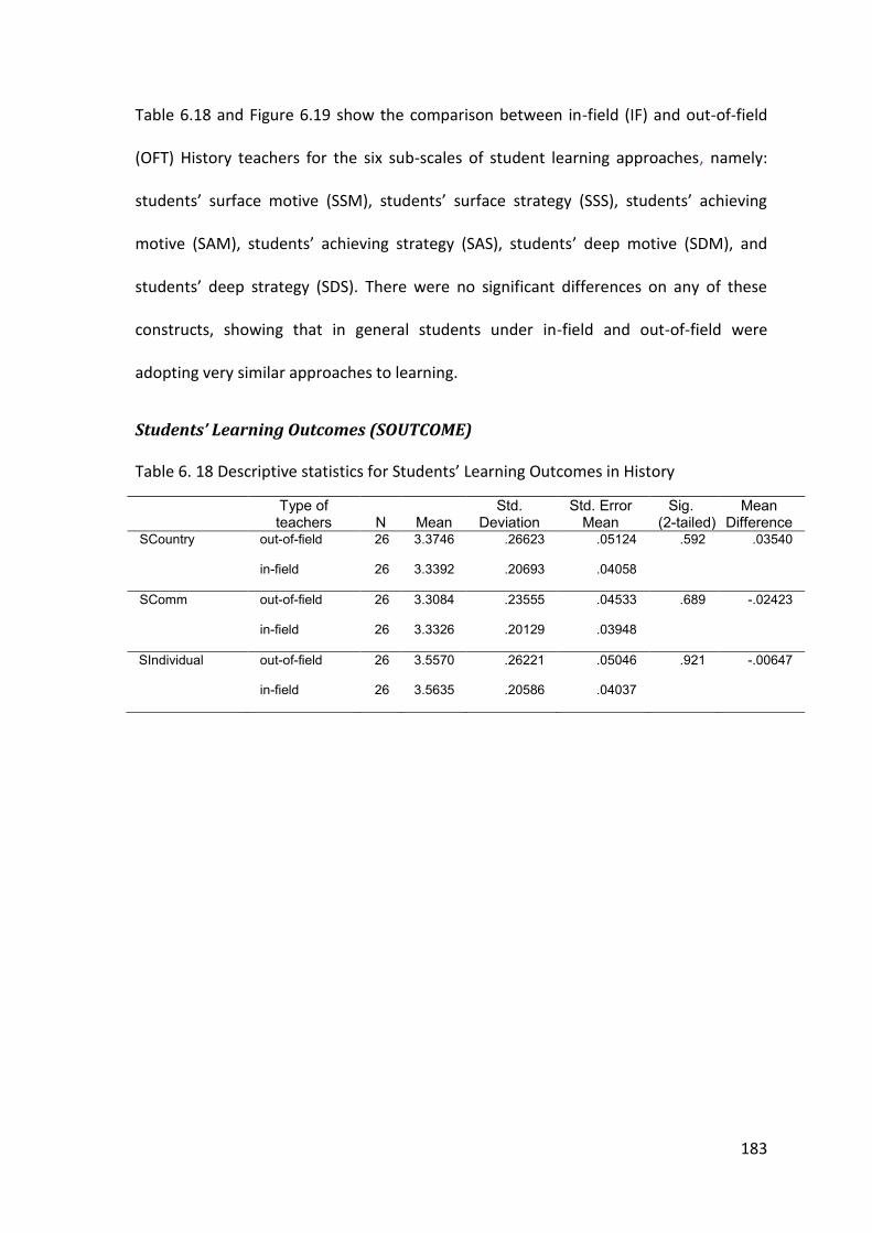
183

Table 6.18 and Figure 6.19 show the comparison between in-field (IF) and out-of-field

(OFT) History teachers for the six sub-scales of student learning approaches, namely:

students’ surface motive (SSM), students’ surface strategy (SSS), students’ achieving

motive (SAM), students’ achieving strategy (SAS), students’ deep motive (SDM), and

students’ deep strategy (SDS). There were no significant differences on any of these

constructs, showing that in general students under in-field and out-of-field were

adopting very similar approaches to learning.

Students’ Learning Outcomes (SOUTCOME)

Table 6. 18 Descriptive statistics for Students’ Learning Outcomes in History


Std. Deviation

Std. Error Mean

Sig. (2-tailed)

Mean Difference

SCountry out-of-field 26 3.3746 .26623 .05124 .592 .03540

in-field 26 3.3392 .20693 .04058

SComm out-of-field 26 3.3084 .23555 .04533 .689 -.02423

in-field 26 3.3326 .20129 .03948

SIndividual out-of-field 26 3.5570 .26221 .05046 .921 -.00647

in-field 26 3.5635 .20586 .04037

184

Figure 6. 20 Students’ Learning Outcomes in History reported by students under in-field and out-of-field teachers.

There were three constructs used to measure students’ learning outcome (SOUTCOME)

namely Country (SContry), Community (SComm) and Individual (SIndividual). Table 6.18

presented the comparison between in-field (IF) and out-of-field (OFT) History teachers

with respect to the students’ learning outcomes. The two-error plots in Figure 6.20

show the mean and the 95% confident intervals of the student learning outcome. There

were no significant differences found for any of the three constructs.


185

6.5 Summary

The information presented in the first part of this chapter shows the demographic

distribution for all respondents, both teachers and students. Over two-thirds (71.7%) of

the teachers were females and two fifths were aged between 31 and 40 years (40%). All

of the teachers had at least a tertiary diploma or university degree from local

universities. Most of the teachers had worked between 2 and 5 years in public schools

in Malaysia and the majority were from the Malay ethnic group.

In the case of the students, most were 16 years old, and more than a half (58.3%) were

female. In terms of ethnicity, almost two-thirds (62.8%) were Malays. Over half of the

mothers were not employed but almost one fifth (17.3%) worked professionally, and

nearly one quarter (23.7%) respondents’ fathers worked at the Service & Sales sectors.

Comparisons between out-of-field and in-field teachers with respect to their own as

well as their students’ characteristics and perceptions were discussed in the second part

of this chapter. The results showed that the in-field teachers had more experience in

teaching History compared to the out-of-field teachers. In terms of teaching

conceptions, the conduct guidance dimension was found to differ significantly, but not

the other dimensions. This indicated that in-field teachers had higher levels of nurturing

good conduct in their students, compared to the out-of-field teachers. In addition, the

results indicated that students under in-field teachers preferred to have classrooms

with higher levels of investigation, personalization, participation and differentiation

activities. In their actual classrooms, students under in-field teachers had experienced

higher levels of personalisation.. The analyses discussed in the next chapter are based

on the results of the descriptive and t-test analyses provided in this chapter.

186

Chapter 7 Partial Least Squares Path

Analysis: Teacher Level ________________________________________________________________________

7.1 Introduction

This chapter reports the partial least squares path analyses of the variables at the

teacher level, in order to determine the pattern of relationships among teachers’

characteristics (age, gender, ethnicity, teacher in-field and out-of-field, and teacher

experience), teachers’ conceptions of teaching, teacher approaches. History teaching

methods, and other compositional variables. These other compositional variables were

aggregated from the student level data which included students’ characteristics (age,

gender, ethnicity), the classroom climate preferred, the classroom climate actual,

approaches to learning (Surface, Achieving and Deep approaches), as well as students’

perceptions of History learning (SOutcomes). The partial least squares path analysis

(PLSPATH) program Version 3.01 (Sellin, 1989) was used in this study. In this chapter,

the background of PLSPATH is explained, the problems in methodology, discussed and

the process of path analysis and its results reported. All the analyses were based on the

teacher data set (52 teachers) and the student data set (1653 students, Form Four).

7.2 Partial Least Squares Path Analysis (PLSPATH)

PLSPATH is a structural equation modelling (SEM) technique that examines structural or

causal models with observed variables (Rintaingrum et al., 2009). Broadly, this

technique is used for estimating the path coefficients in path models with latent

constructs measured by multiple indicators. PLSPATH is particularly useful in situations

187

with large amounts of data and a lack of theoretical knowledge. PLSPATH, does not

require stringent distributional assumptions, such as normality. It is referred to as a ‘soft

modelling’ approach, which is useful in research which is exploratory in nature (Sellin,

1995).

Path analysis requires the development of an appropriate structural or causal model

and the testing of that model (Falk & Miller, 1992; Sellin 1989; 1995). A model in

quantitative studies comes in two forms, either in a series of structural equations or in

a graphic description which represents the variables in the study. Byrne (2001) stressed

that using the diagrams enables a clearer understanding of the theory. AMOS 17

(Arbuckle, 2008), was used to draw the path diagrams in this study by incorporating the

paths coefficients provided by PLSPATH results. Generally, there are four shapes

involved in drawing the path diagram; (1) circles or ellipses represent unobserved

variables (latent variables), (2) rectangles represent observed variables (manifest

variables), (3) single headed arrows represent the impact of one variable on one or

more other variables , and (4) double-headed arrows represent covariances or

correlations between two of variables (Byrne, 2010).

Inner model and outer model

Two different models of variables are involved in the PLSPATH diagrams. The inner

model refers particularly to the relationships between unobserved or latent variables

(LVs) - structural model. The outer model specifies the relationships between LVs and

their associated observed or manifest variables (MVs) or know as measurement model.

(Sellin, 1995). With this technique, relationships between the variables can be divided

into two categories. The first category is where the constructs (LVs) are viewed as the

188

cause of the measures. These relationships are labelled as “reflective”, or the

manifestations of a construct. Arrows which are drawn from LVs to MVs, known as the

outward mode arrows, indicate this relationship. The second relationship category is

referred to as “formative”, where the measures are viewed as the cause of the

constructs. Formative relationships are indicated by arrows drawn from MVs to the LVs;

these are known as inward mode arrows.

Variables Mode & Types of Variables

Generally there were three modes of the variables in the path diagrams. The latent

variable can be in the inward mode, in the outward mode, or involved in unity mode

with only one manifest variable.

There are three types of variables involved in a model. They are referred to as

exogenous, endogenous and criterion variables. The variables that are not dependent

on any other variables are referred as exogenous. A variable can be recognised as

exogenous when there are no unidirectional arrows pointing towards it. Endogenous

variables are dependent on other variables, a relationship indicated by one or more

unidirectional arrows pointing to them. Criterion variables are those which are

dependent only on other variables (Rintaningrum et al., 2009).

Indices

In this technique, loadings and weights are commonly used to indicate the strength of

the relationships between the MVS and LVs. According to Sellin and Keeves (1997), the

loadings should be reported where the outward mode is used, and weights should be

reported where the inward mode is used. In addition, there are a number of indices,

such as, beta, jackknife mean, jackknife standard error and correlation which are used

189

to indicate the strength of the paths or relationships in the inner (structural) model in

the PLSPATH analyses.

Procedure

The PLSPATH parameter estimation proceeds in two steps. The first step involves the

iterative estimation of latent variables (LVs) as linear composites of their associated

manifest variables (MVs). The second step involves the non-iterative estimation of inner

model and outer model coefficients. In the second step of PLSPATH analysis, the

estimated LVs from the first step are used to estimate the inner model coefficients by

means of the standard least square procedure. Thus for recursive inner model (Keeves,

1997) the inner model coefficients are obtained by ordinary least square (OLS)

regression, applied to each inner model equation separately. In doing this, the relations

between LVs in the path model or inner model indicate causal relationships between

LVs. A unidirectional arrow from the determining variables to the dependent variables

indicates this relationship.

Advantages of PLSPATH analysis

PLSPATH was chosen for this study because it has many advantages. As a statistical

technique, Sellin and Keeves, (1997) claimed that PLSPATH analysis; (a) is flexible and

robust in testing complex models, (b) does not require rigorous distributional

assumptions of variables; (c) accepts both continuous and dichotomous variables and (d)

recognises cluster sample designs in data, as is the case for this study. Moreover,

PLSPATH analysis has been described as a soft- modeling approach which could be

useful in the investigation of causal-predictive analysis rather than confirmatory analysis

(Sellin & Keeves, 1997). In other words, this analysis is less theory-based and more

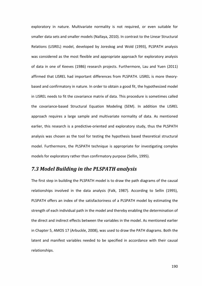
190

exploratory in nature. Multivariate normality is not required, or even suitable for

smaller data sets and smaller models (Nallaya, 2010). In contrast to the Linear Structural

Relations (LISREL) model, developed by Joreskog and Wold (1993), PLSPATH analysis

was considered as the most flexible and appropriate approach for exploratory analysis

of data in one of Keeves (1986) research projects. Furthermore, Lau and Yuen (2011)

affirmed that LISREL had important differences from PLSPATH. LISREL is more theory-

based and confirmatory in nature. In order to obtain a good fit, the hypothesized model

in LISREL needs to fit the covariance matrix of data. This procedure is sometimes called

the covariance-based Structural Equation Modeling (SEM). In addition the LISREL

approach requires a large sample and multivariate normality of data. As mentioned

earlier, this research is a predictive-oriented and exploratory study, thus the PLSPATH

analysis was chosen as the tool for testing the hypothesis based theoretical structural

model. Furthermore, the PLSPATH technique is appropriate for investigating complex

models for exploratory rather than confirmatory purpose (Sellin, 1995).

7.3 Model Building in the PLSPATH analysis

The first step in building the PLSPATH model is to draw the path diagrams of the causal

relationships involved in the data analysis (Falk, 1987). According to Sellin (1995),

PLSPATH offers an index of the satisfactoriness of a PLSPATH model by estimating the

strength of each individual path in the model and thereby enabling the determination of

the direct and indirect effects between the variables in the model. As mentioned earlier

in Chapter 5, AMOS 17 (Arbuckle, 2008), was used to draw the PATH diagrams. Both the

latent and manifest variables needed to be specified in accordance with their causal

relationships.

191

Based on the theoretical framework adapted from the Biggs’ Model of Learning (1987)

(see Chapter 2) it was purposed that there were three groups of factors involved in

learning: presage, process and product. The presage factors were the student

characteristics (age, gender, and ethnicity), classroom environment (actual and

preferred), and as well as the teacher characteristics (age, gender, ethnicity), in-field,

out-of-field, and experiences), teaching approaches, teaching methods and teaching

conceptions. The process factor related to students’ learning approaches (Surface, Deep

and Achieving), and the product factor was the achievement of the History learning

objective as perceived by the students.

All factors in the model are related to the hypothesised process factor of students’

approaches to learning, which in turn is hypothesised to be linked to the products.

Students’ perceptions of learning objective in History (country, community, and

individual) were proposed as the outcome in this study. All the presage, process and

products are included in the path model. Consequently, in the inner model there are 15

latent variables and 42 manifest variables. The hypothesised paths for estimating the

relationships between teacher and student variables are displayed in Figure 7.1 and 7.2.

As mentioned earlier there are three types of latent variables in PLSPATH; (1)

exogenous (independent) variables, which receive no causal inputs from other variables,

(2) endogenous (dependent) variables, which receive one or more causal inputs from

other variables, (3) criterion variables, which depend only on other variable

(Rantaningrum et. al., 2009).Independent variables are also known as antecedent

variables, as they are not influenced by other latent variables (LVs).

192

In this study the exogenous (independent) variables for the teacher level were teachers’

age, gender, ethnicity, and years of teaching; for the student level, they were students’

age, gender, ethnicity, in-field, and out-of-field History teachers. The endogenous

(dependent) variables for the teacher level were teaching approaches, History teaching

methods and teaching conceptions, while for student they were classroom environment

(actual and preferred), learning approaches (Surface, Deep and Achieving). The criterion

variables were the product factors: students’ learning objectives in History as a subject

(country, community, and individual). The full list of the variables in this study is

presented in Tables 7.1 and Table 7.2 in relation to the two Hypothesised Models 1 and

2 labelled Figures 7.1 and 7.3; and the Final Models labelled 1 and 2 as presented in

Figures 7.2 and 7.4.

193

Table 7. 1 Variables at the Teacher Level - Model 1

Latent Variable (Acronym)

Mode Description Manifest Variables (Acronym)

Description Coding

TAge unity Teacher’s age TYear Age in years 21-50

TGender unity Teacher’s gender TGdr 0=Male 1= Female 0=M 1=F

TEthnic Inward Teacher’s ethnicity Malay Malay (Dummy) 0=Not Malay 1=Malay

Chinese Chinese 0=Not Chinese 1=Chinese Indian Indian 0=Not Indian 1=Indian Other Iban/Melanau/Thai 0=Not Other 1=Other TInout unity Teacher's qualification In-field In-field/ out of-field 0= 0ut of-field 1= In-field TExp unity Teacher Years of teaching Tytea Teaching experience

in History Raw Scores

TApp outward Teaching approaches TInfoTra Information Transfer Factor Scores TConChan Conceptual Change Factor Scores

TMet outward Teaching Methods TEft Teaching Effective Factor Scores Tact Teaching Active Factor Scores

TCont outward Teaching Conception TExam Exam Preparation Factor Scores TKDeli Knowledge Delivery Factor Scores

TAttPro Attitude Promotion Factor Scores

TAbiDev Ability Development Factor Scores

ConDance Conduct Guidance Factor Scores

SAge unity Student’s age SYear Age in years 17-18

SGender unity Student’s gender SGdr 0=Male 1= Female 0=M 1=F SEthnic Inward Student’s ethnicity Malay Malay (Dummy) 0=Not Malay 1=Malay

Chinese Chinese 0=Not Chinese 1=Chinese Indian Indian 0=Not Indian 1=Indian Other Iban/Melanau/Thai 0=Not Other 1=Other SCCA outward Classroom Climate Actual Spar Participation Factor Scores Sind Independence Factor Scores

SPer Personalisation Factor Scores

SInv Investigation Factor Scores

SDfr Differentiation Factor Scores

SCCP outward Classroom Climate Preferred SINV Investigation Factor Scores

SPER Personalisation Factor Scores

SPARTICI Participation Factor Scores

SINDEPEN Independence Factor Scores

SDIFFER Differentiation Factor Scores

SLearning outward Student’s Approaches to Learning

SSM Surface Motive Factor Scores

SSS Surface Strategy Factor Scores

SAM Achieving Motive Factor Scores

SAS Achieving Strategy Factor Scores

SDM Deep Motive Factor Scores

SDS Deep Strategy Factor Scores

SOutcome outward Students’ Perception of History Learning

SCountry Appreciating country Factor Scores

SCommunity Appreciating society Factor Scores

SIndividual Enhance maturity & moral value

Factor Scores

194

Figure 7. 1 Hypothesised Model for Teachers’ Level Model 1

195

Figure 7. 2 Final Model for Teachers’ Level Model 1

TMet

TExp

TGender

TInout

TCont

SEthnic

CCA

SGdr CCP

Learning

Outcome

TEft TAct SGDR

SSM

SSS

SAM

SCountry

SCommu

SIndivid

SPar0.94

SInd-0.46

SPer0.01

SInv0.8

SDfr-0.22OtherIndianChineseMalay

TExam

0.86

TKDeli0.9

TAttPro

0.84

TAbi

0.93

Condanc

0.9

SINV

0.8

SPER SPARTICI INDEPEN

-0.36

SDIFFER

TAge

TGdr

TYear

Infield

Tyrtea1

TAppTConChan 0.95

TInfoTra

1

SAS

SDM

SDS

10.98 -0.92

0.99

.18(.14)

.38(.14)

-.47(.09)

.30(.11)

0.12

.34(.12)

0.98

0

.22(.13)

1

1

.89(.04) .12(.04)

0.90.97

.33(.13)

.66(.09).46(.11)

.32(.13)

.27(.10)

.18(.08)

-.36(.13)

0.860.07

0.970.94

0.97

0.93

0.98

0.99

0.99

.84(.05)

0.9

0.02

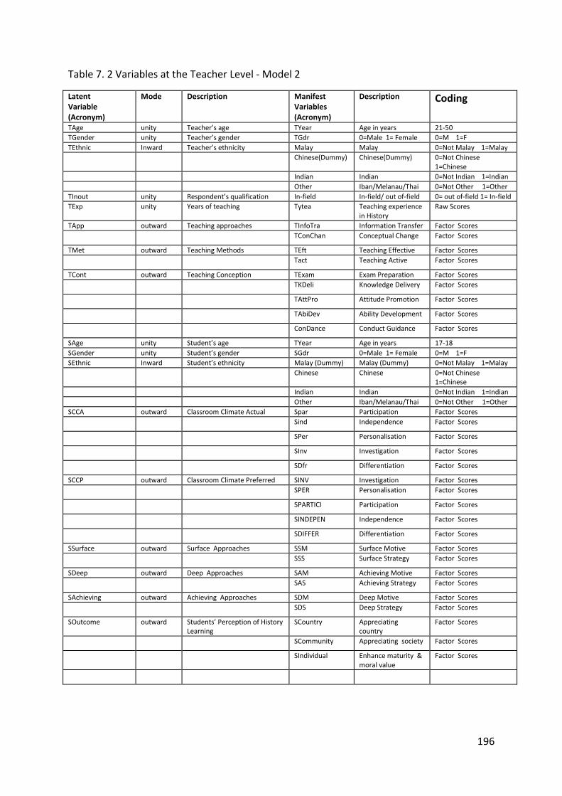
196

Table 7. 2 Variables at the Teacher Level - Model 2



Description Coding



TEthnic Inward Teacher’s ethnicity Malay Malay 0=Not Malay 1=Malay

Chinese(Dummy) Chinese(Dummy) 0=Not Chinese 1=Chinese

Indian Indian 0=Not Indian 1=Indian Other Iban/Melanau/Thai 0=Not Other 1=Other TInout unity Respondent’s qualification In-field In-field/ out of-field 0= out of-field 1= In-field TExp unity Years of teaching Tytea Teaching experience



TMet outward Teaching Methods TEft Teaching Effective Factor Scores Tact Teaching Active Factor Scores





SAge unity Student’s age TYear Age in years 17-18

SGender unity Student’s gender SGdr 0=Male 1= Female 0=M 1=F

SEthnic Inward Student’s ethnicity Malay (Dummy) Malay (Dummy) 0=Not Malay 1=Malay

Chinese Chinese 0=Not Chinese 1=Chinese

Indian Indian 0=Not Indian 1=Indian Other Iban/Melanau/Thai 0=Not Other 1=Other SCCA outward Classroom Climate Actual Spar Participation Factor Scores Sind Independence Factor Scores




SCCP outward Classroom Climate Preferred SINV Investigation Factor Scores SPER Personalisation Factor Scores




SSurface outward Surface Approaches SSM Surface Motive Factor Scores SSS Surface Strategy Factor Scores

SDeep outward Deep Approaches SAM Achieving Motive Factor Scores SAS Achieving Strategy Factor Scores

SAchieving outward Achieving Approaches SDM Deep Motive Factor Scores SDS Deep Strategy Factor Scores


SCountry Appreciating country

Factor Scores



Factor Scores

197

Figure 7. 3 Hypothesised Model for Teachers’Level Model 2

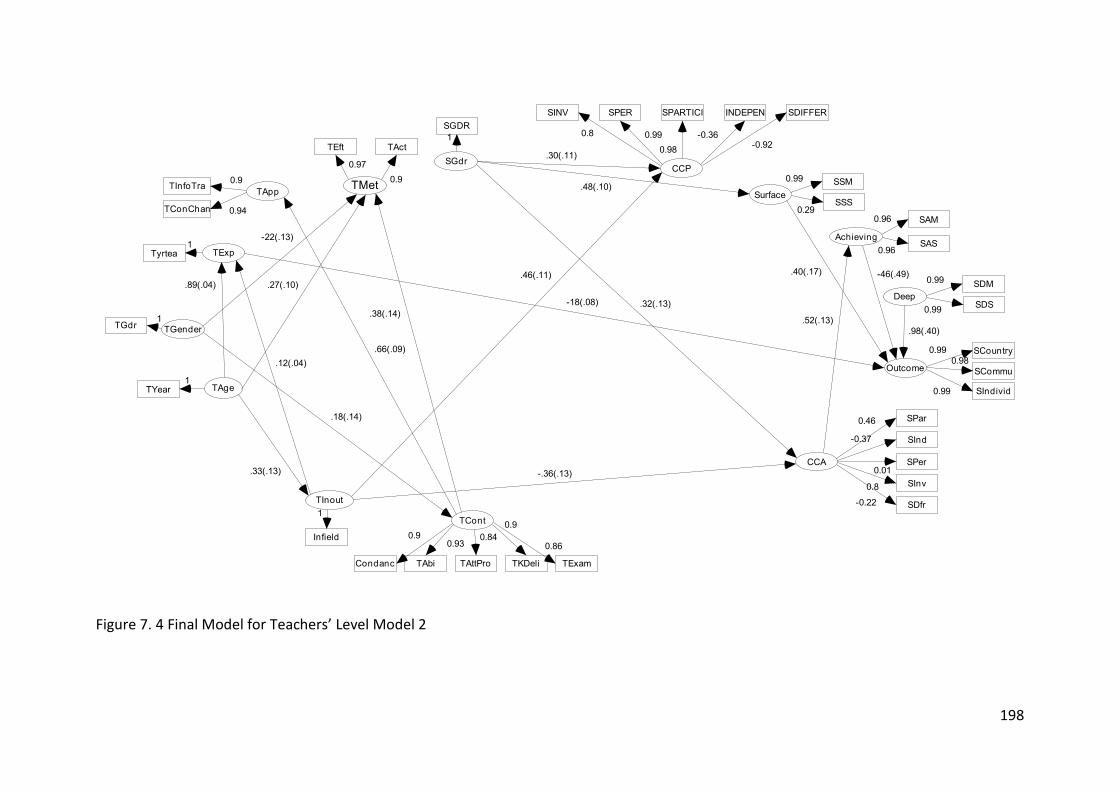
198

Figure 7. 4 Final Model for Teachers’ Level Model 2

TMet

TExp

TGender

TInout

TCont

CCA

SGdrCCP

Deep

Outcome

TEft TAct

SGDR

SSM

SSS

SAM

SCountry

SCommu

SIndivid

SPar0.46

SInd-0.37

SPer0.01

SInv0.8

SDfr-0.22

TExam

0.86

TKDeli

0.9

TAttProTAbi

0.93

Condanc

0.9

SINV

0.8


-0.36

SDIFFER

TAge

TGdr1

TYear1

Infield

Tyrtea1

TApp

TConChan 0.94

TInfoTra 0.9

1

SAS

SDM

SDS

10.98 -0.92

0.99

.18(.14)

Surface

Achieving

.52(.13)

.40(.17)

0.970.9 0.99

0.96

0.96

0.99

0.99

0.980.99

0.99

.98(.40)

.46(.11)

.38(.14)

.48(.10)

0.84

.12(.04)

.30(.11)

.66(.09)

.32(.13)

0.29

-.36(.13)

-46(.49)

-18(.08)

-22(.13)

.27(.10).89(.04)

.33(.13)

199

The difference between Teachers’ level Model 1 and Model 2 relates to the

representation of the ‘Learning Approaches’ variable; In Model 1, all these variables

were combined into one student learning approach ‘SLearning’ In Model 2, the

‘Learning Approaches’ variables were represented as separate variables: surface motive,

deep motive, achieving motive, surface strategy, deep strategy, achieving strategy. The

results of the PLSPATHS analysis are discussed in the rest of the chapter.

7.4 Outer Model–Teachers’ Level Models 1 & 2

The outer model or measurement model indicates the relationships between the latent

variables and the manifest variables. These relationships have three possible modes

(types): (1) formative mode, (2) reflective mode and, (3) unity mode (Darmawan, 2003,

Rintaningrum et al., 2009). Any manifest variable that does not contribute to the

formation or reflection of a latent variable needs to be removed from the further

analyses. In PLSPATH, ‘PATTERN’ is the command line that refers to the relationship

between latent variables and their manifest variables.

Despite having many advantages as discussed earlier, PLSPATH also has a few

limitations. One of the limitations, claimed by Darmawan (2003, p. 810), is ‘the lack of

any test of significance’. However, Sellin (1989) suggested that jackknife methods which

provide the estimate of the standard error could be used as a test of significance for the

results. Furthermore, Sellin (1989) suggested the use of the ‘Stone-Geisser’ test which

predicts relevance. This test, ‘basically produces jackknife estimates of residuals

variances while jackknife standard errors of points estimates can be obtained as by-

products. The general idea is to omit one case at time, to re-estimate the model

200

parameters on the basis of the remaining cases, and to reconstruct or predict omitted

case values using the re-estimated parameters’ (Sellin,1989, p.262).

In the PLSPATH analysis, five coefficients are used as indicators to delete a manifest

variable from a latent construct. The five indices are: (1) weight, (2) loadings, (3)

communality, (4) redundancy, and (5) tolerance. The fit indices for teachers’ Models 1

and 2 are presented in Table 7.3. The discussion of the results is based on these indices.

The weight indices are the strength of the regression relationships between LVs and

MVs in the inward or formative mode. Relationships between LVs and MVs are

considered meaningful if the values of the associated weight are equal to or greater

than 0.10 (Sellin & Keeves, 1997). Where a weight of zero is recorded, the MV acts as a

reference in the use of dummy variables for regressions analyses. In this study there

were initially two inward mode latent variables, namely TEthnic and SEthnic. Since the

LVs for TEthnic in both models showed no relationship with other constructs. In other

words, there were no unidirectional arrows pointed towards the variables, showing that

there were no causal relationships between the LVs and MVs. Therefore, it was

removed from both models. In the case of SEthnic, the results led to its deletion in

Model 2, since it had no significant on other constructs, however, the variable of SEthnic

was found to have a significant effect on the ‘Learning’ construct in Model but justified

it being retained in Model 1. Another criteria on, used for the outer model indices, is

factor loading. Factor loading indicates the strength of factor analytic relationships

between MVs and LVs in the outward or reflective mode (Sellin & Keeves, 1997). There

were seven outward (reflective) mode latent variables in this model. A value equal to or

larger than 0.40 is considered an adequate factor loading value (Sellin & Keeves, 1997).

201

Negative loadings indicate that the corresponding manifest variables (MVs) are in the

opposite direction on the scale, compared to the MVs that have positive loadings.

Negative loadings indicated that the corresponding manifest variables (MVs) are in the

opposite direction on the scale, compared to the MVs that have positive loadings.

Communality indicates the strength of the outer model and is calculated as the squared

correlation between MVs and their associated latent variables (Sellin, 1989). Falk (1987)

claimed that the strength of the outer model is measured by the average of the

communality values. He added that, if the communality values are greater than 0.30,

the values are considered as significantly strong. The higher the average for the

communality index, the better the outer model (Falk, 1987). Redundancy indicates the

joint predictive power of inner model and outer model relationships as estimated for a

given data set (Sellin, 1989). Tolerance indicates the possible multicollinearity within the

corresponding block of MVs. Tolerance is calculated as the squared correlation between

a given MV and the remaining MVs belonging to the same LV (Sellin, 1995). It is

commonly accepted (Sellin, 1989) that if the tolerance value is 0.50 or higher, it can be

considered that adequate multicollinearity exists within the block of MVs. According to

Darmawan (2003), tolerance indicates the possibility of seriously damaging

multicollinearity within the corresponding block of MVs. However these effects can be

considered to damage the inward (formative) mode rather than the outward (reflective)

mode. In this recent study, the multicollinearity was strong for the block with outward

mode, but not for the block with the inward mode, as expected. In the outward mode,

all MVs are expected to be highly correlated to one another, in contrast to the inward

mode in which low correlations among MVs are expected.

202

Table 7. 3 Indices for the Outer Model – Teachers’ Level Model 1 and Model 2

MODEL 1 MODEL 2

Variables Mode W L C R T W L C R T

TAGE/Tyears unity 1 1 1 0 0 1 1 1 0 0

TGENDER/TGdr unity 1 1 1 0 0 1 1 1 0 0

TInout unity 1 1 1 0 0 1 1 1 0 0

TExp unity

Tyrteac 1 1 1 0 0 1 1 1 0 0

TApp outward TInfoTra 0.45 0.90 0.82 0.36 0.52 0.45 0.90 0.82 0.36 0.52

TConChan 0.62 0.94 0.90 0.40 0.52 0.62 0.94 0.90 0.40 0.52

TMet outward

TEft 0.67 0.97 0.93 0.29 0.59 0.67 0.97 0.93 0.29 0.59

TAct 0.40 0.90 0.82 0.25 0.59 0.40 0.90 0.82 0.25 0.59

TCont outward

TExam 0.27 0.86 0.74 0.02 0.61 0.27 0.86 0.74 0.02 0.61

TKDeli 0.23 0.90 0.81 0.03 0.72 0.23 0.90 0.81 0.03 0.72

TAttPro 0.16 0.84 0.70 0.02 0.66 0.16 0.84 0.70 0.02 0.66

TAbiDev 0.25 0.93 0.86 0.03 0.78 0.25 0.93 0.86 0.03 0.78

ConDance 0.23 0.89 0.81 0.03 0.75 0.23 0.89 0.81 0.03 0.75

Sage/ years unity 1 1 1 0 0 SGender /sex unity 1 1 1 0 0 SEthnic inward Malay (D) 0 0 0 0 0 Chinese 0.96 0.99 0.97 0.00 0.06 0.96 0.99 0.97 0.00 0.06

Indian 0.18 0.35 0.12 0.00 0.05 0.18 0.35 0.12 0.00 0.05

Other -0.04 0.17 0.03 0.00 0.05 -0.04 0.17 0.03 0.00 0.05

SCCA outward

SPar 0.91 0.94 0.89 0.16 0.60 0.91 0.94 0.89 0.16 0.60

Sind 0.06 -0.46 0.21 0.04 0.44 0.06 -0.46 0.21 0.04 0.44

SPer -0.17 0.01 0.64 0.12 0.69 -0.17 0.01 0.64 0.12 0.69

SInv 0.27 0.80 0.64 0.12 0.68 0.27 0.80 0.64 0.12 0.68

SDfr 0.22 -0.22 0.05 0.01 0.32 0.22 -0.22 0.05 0.01 0.32

SCCP outward

SINV 0.20 0.80 0.64 0.19 0.83 0.20 0.80 0.64 0.19 0.83

SPER 0.29 0.99 0.98 0.30 0.99 0.29 0.99 0.98 0.30 0.99

SPARTICI 0.27 0.98 0.95 0.28 0.99 0.27 0.98 0.95 0.28 0.99

SINDEPEN -0.17 -0.36 0.13 0.04 0.65 -0.17 -0.36 0.13 0.04 0.65

SDIFFER -0.25 -0.92 0.85 0.25 0.89 -0.25 -0.92 0.85 0.25 0.89

SOutcome outward SCountry 0.33 0.99 0.97 0.74 0.94 0.33 0.99 0.97 0.74 0.94

SCommunity 0.34 0.98 0.97 0.74 0.93 0.34 0.98 0.97 0.74 0.93

SIndividual 0.34 0.99 0.99 0.75 0.96 0.34 0.99 0.99 0.75 0.96

SLearning outward SSM 0.22 0.87 0.76 0.31 0.97 SSS 0.03 0.07 0.001 0.002 0.80 SAM 0.23 0.98 0.95 0.39 0.98 SAS 0.20 0.94 0.89 0.36 0.99 SDM 0.23 0.97 0.94 0.38 0.99 SDS 0.20 0.93 0.87 0.35 0.99 Surface outward SSM 1.02 0.99 0.99 0.99 0.12

SSS -0.07 0.29 0.08 0.08 0.12

Achiev outward

SAM 0.51 0.96 0.93 0.25 0.73

SAS 0.52 0.96 0.93 0.25 0.73

Deep outward

SDM 0.52 0.99 0.97 0.00 0.90

SDS 0.49 0.99 0.97 0.00 0.90

Notes: W =Weight, L= Loadings, C= communality, R= Redundancy and T= Tolerance

203

Discussion - Outer Models Model 1 and 2

The discussion below focuses on each of the variables in the outer model of the two

Teachers’ Level Path diagrams (see Figures 7.1 and 7.2). These two Path diagrams share

the same variables, except in the case of the Students’ Learning Approaches: SLearning

from Path Diagram Model 1 and SURFACE, ACHIEVING and DEEP in Path Diagram Model

2. The discussion of this last variable occurs at the end of the sections.

Teachers Age (TAge)

Teacher’ age (TAge) as a latent variable was formed out of a single manifest variable,

namely TYear. In the model, the TYear variable was reflected by a single indicator and

the value of its loading was 1.00 (unity).

Teachers’ Gender (TGender)

Teachers Gender (TGender) was similar reflected by a single indicator namely, TGdr. The

value of its loading was 1.00 (unity).

Teacher Qualifications (Tinout)

Teacher in-field and out-of-field teachers (Tinout) was also reflected by a single

indicator namely, TInfield. The value of its loading was 1.00 (unity).

Teachers’ Experience (Tyrtea)

Teacher experience (TExp) was also reflected by a single indicator namely, Tyrtea. The


204

Student Age (SAge)

Student age (SAge) as a latent variable was formed out of a single manifest variable.,

namely SYear. In the model, the SAge variable was reflected by a single indicator and


Students’ Gender (SGender)

Students’ Gender (SGender) was also reflected by a single indicator namely, SGdr. The

value of its loading was 1.00 (unity)

Students’ Ethnicity (SEthnic)

Students’ Ethnicity (SEthnic) was formed by four MVs that represent the four ethnic

groups the students belong to Malay, Chinese, Indian and Other. In this model, the

Malay group was used as a reference point (Dummy). Therefore, the factor weight for

Malay was set to 0. The regression weight for the three other groups were 0.99, 0.35

and 0.17, for Chinese, Indian, and other.

Teacher Approaches (TApp)

Teacher Approaches (TApp) was a latent variable which was reflected by only two MVs,

namely information transfer or teacher-focused (TInfoTra) and conceptual change or

student-focused (TConChan). As an outward latent construct, TApp was strongly

reflected by these two MVs, with factor loadings of 0.90 and 0.94.


Teaching Methods (TMet) construct was also reflected by two MVs namely, teaching

effective (TEft) and teaching active (TAct). These two MVs were composite scores

calculated using a principal component method. The way in which these MVs were

formed is explain Chapter 5. These two MVs had high factor loadings (0.97 and 0.90)

205

indicating that this construct was strongly reflected by the two MVs. Factor loadings

were similar for both models.

Teacher Conceptions (TCont)

Five MVs reflected the construct of Teacher Conceptions (TCont), namely Exam

preparation (TExam), Knowledge delivery (TKDeli), Attitude promotion (TAttPro), Ability

development (TAbiDev) and Conduct guidance (ConDance). The factor loadings which

were 0.86, 0.90, 0.84, 0.93 and 0.90 respectively were regarded as moderate to high.

These results indicate that all MVS were found to be strong reflectors of the construct.

Students Classroom Climate Actual (SCCA)

Students’ Classroom Climate Actual (SCCA) was an outward latent variable reflected by

five MVs, namely Student Participation (Spar), Student Independence (Sind), Student

Personalisation (SPer), Student Investigation (SInv) and Student Differentiation (SDfr).

The factor loadings were 0.94, -0.46, 0.01, 0.80 and -0.22 respectively for both models.

These coefficients indicated that the SCCA were strongly reflected by Student

Participation (Spar) and Student Investigation (SInv). Personalisation was found to be a

very strong reflector of SCCA in the Malaysian context. On the other hand, Investigation

and Differentiation had negative coefficients. The negative loadings indicated that the

corresponding manifest variables were in the opposite direction on the scale compared

to those MVs that had positive loadings. For examples, those classes which were high

on Participation and Investigation would have correspondingly low scores for

Independence and Differentiation.

206

Students’ Classroom Climate Preferred (SCCP)

Similar to the Classroom Climate Actual, Students’ Classroom Climate Preferred (SCCP)

was also reflected by five MVs namely Student Investigation (SINV), Student

Personalisation (SPER), Student Participation (SPARTICI), Student Independence

(SINDEPEN), and Student Differentiation (SDIFFER). The MVs’ factor loadings were

strong for SINV, SPER, SPARTICI, and SDIFFER (0.80, 0.99, 0.98, and -0.92) and moderate

for SINDEPEN (-0.36).

Students’ Learning Outcomes (Outcome)

Students’ Learning Outcomes (Outcome) was reflected by Student Country (SCountry),

Student Community (StudentCommunity), and Student Individual (SIndividual). These

three MVs had high factor loadings 0.99, 0.98, and 0.99 respectively for both models.

This result indicates that this construct was strongly reflected by the three MVs.

Student Learning (SLearning)

Student Learning (SLearning) was an outward mode latent variable reflected by six MVs,

namely Student Surface Motive (SSM), Student Surface Motive (SSM), Student Achieving

Motive (SAM), Student Achieving Strategy (SAS), Student Deep Motive (SDM), Student

Deep Strategy (SDS). All MVs were strong reflectors of the construct, with loading

ranging from 0.07 to 0.98. SAM was found to be the strongest reflector of this construct.

This construct is only in Model 1.

SURFACE (Surface)

SURFACE was reflected by only two manifest variables namely, Student Surface Motive

(SSM) and Student Surface Strategy (SSS). As an outward latent construct, SURFACE was

207

reflected by these two MVs, with the factor loadings of 0.99 and 0.29 respectively. This

construct appeared only in Model 2.

ACHIEVING (Achiev)

In similar manner to SURFACE, ACHIEVING (Achiev) was reflected by two MVs namely,

Student Achieving Motive (SAM) and Student Achieving Strategy (SAS). Both MVs were

strong reflectors of achieving, with factor loadings of 0.96 and 0.96. This construct also

was only in Model 2.

DEEP

DEEP was reflected by only two MVs variables namely, Student Deep Motive (SDM),

Student Deep Strategy (SDS). As an outward latent construct, DEEP was strongly

reflected by these two MVs, with the factor loadings of 0.99 and 0.99 respectively. This

construct appeared only in Model 2.

7.5 Inner Model –Teachers’ Level Path Model 1 and 2

The inner or structural model indicates the relationships between one LV regressed on

other LVs (Rintaningrum et al., 2009). In PLSPATH version 3.01, these relationships are

termed ‘MODEL’ in the command line. Any paths between the LVs are removed from

the further analysis, if the path does not show meaningful and adequate influence

(Darmawan, 2003; Rintaningrum et al., 2009). The indicators which are used in the

analysis of the inner model to delete or remove the non-significant path (a) regression

coefficient (beta), (b) correlation coefficient (r), (c) tolerance, (d) jackknife means

(JknMean), and (e) jackknife standard error(JknStd). To check the predictive strength of

the inner model, R-squared (R²) is used.

208

Beta is the coefficient of the direct effect between one latent variable and another.

Sellin (1989) suggested that the beta coefficient is generally acceptable with a value of

0.05 or larger, for a large data set, or 0.10 for a small data set. The jackknife mean is the

mean of the path coefficients obtained in each jackknife cycle. The jackknife standard

error is the estimated error associated with each path coefficient. Correlation

coefficients involve zero-order or product moment correlation coefficients between the

given independent (predictor) latent variable and the dependent (criterion) latent

variable (Sellin, 1989).

Although, in PLSPATH analysis, a statistically significant test is not provided as part of

the results, Darmawan (2003, p. 82), argued that ‘where an estimated coefficient is

more than twice the value of its jackknife standard error, the coefficient can be

considered to be statistically significant at approximately the five per cent level of

probability’.

Sellin and Keeves (1997) suggested that a direct path with a coefficient of β<0.10 could

be deleted because such a value indicated a less meaningful effect on the estimation of

the relationship between the two LVs. In fact, the greater the β value, the greater is the

effect on the path model. For this study the process was continued until all inadequate

paths were removed. Table 7.4 presents the remaining path indices for the inner model

in relation to Model1 and 2.

209

Table 7. 4 Path Indices for PLS Inner Model – Model 1 and Model 2

MODEL 1 MODEL 2 Variable

Beta JknMean JknStd Corr Tolerance Beta JknMean JknStd Corr Tolerance

Teacher in-field/out-of field (TINOUT) Teacher Age (TAGE) 0.33 0.33 0.13 0.33 0.00 0.33 0.33 0.13 0.33 0.00

Teaching Conception (TCONCEPT) Teacher Gender (TGENDER) 0.18 0.18 0.14 0.18 0.00 0.18 0.18 0.14 0.18 0.00

Teacher Approaches (TAPPROAC) Teacher Conception (TCONCEPT) 0.66 0.66 0.10 0.66 0.00 0.66 0.66 0.10 0.66 0.00

Teaching Method (TMETHOD) Teacher Gender (TGENDER) 0.22 0.22 0.13 0.27 0.04 Teacher Age (TAGE) 0.27 0.27 0.10 0.28 0.02 Teacher Conception (TCONCEPT) 0.38 0.38 0.14 0.45 0.04 0.26 0.26 0.18 0.46 0.43 Teacher Approaches (TAPPROAC) 0.30 0.30 0.19 0.48 0.43

Teacher Year of Teaching (TEXP) Teacher Age (TAGE) 0.89 0.89 0.04 0.93 0.11 0.89 0.89 0.04 0.93 0.11 Teacher in-field/out-of field (TINOUT) 0.12 0.12 0.06 0.41 0.11 0.12 0.12 0.06 0.41 0.11

Classroom Climate Preferred (CCP) Teacher in-field/out-of field (TINOUT) 0.46 0.46 0.11 0.45 0.05 0.46 0.46 0.11 0.45 0.05 Student Gender (SGENDER) 0.30 0.30 0.11 0.30 0.05 0.30 0.30 0.11 0.30 0.05

Classroom Climate Actual (CCA) Teacher in-field/out-of field (TINOUT) -0.35 -0.35 0.13 -0.37 0.05 -0.35 -0.35 0.13 -0.37 0.05 Student Gender (SGENDER) 0.32 0.32 0.13 0.24 0.05 0.32 0.32 0.13 0.24 0.05

Students’ Perception of History Learning (SOUTCOME)

Student Learning Approaches (LEARNING) 0.84 0.84 0.05 0.86 0.11 Teacher Year of Teaching (TEXP) 0.18 0.18 0.08 0.26 0.11 Surface Learning Approaches (SURFACE) 0.40 0.40 0.17 0.74 0.86 Achieving Learning Approaches (ACHEIV) -0.46 -0.46 0.49 0.85 0.98 Deep Learning Approaches (DEEP) 0.98 0.98 0.40 0.85 0.96

Student Approaches to Learning (SLEARNING) Student Gender (SGENDER) 0.34 0.34 0.12 0.44 0.04 Student Ethnicity (SETHNIC) -0.48 -0.48 0.10 0.44 0.04

Surface Learning Approaches (SURFACE) Student Gender (SGENDER) 0.39 0.48 0.17 0.48 0.00

Achieving Learning Approaches (ACHIEV) Classroom Climate Actual (CCA) -0.46 0.52 0.49 0.52 0.00

210

Table 7. 5 Summary of Direct, Indirect and Total Effects for the Inner Model – Model 1 and Model 2

MODEL 1 MODEL 2

Dependent Direct Indirect Total Correlation Direct Indirect Total Correlation

Independent β i β + i r β i β + i r

Variables

TINOUT R² = 0.11 R² = 0.11 TAGE 0.33 - 0.33 0.33 0.33 - 0.33 0.33

TCONCEPT R² = 0.32 - R² = 0.32 TGENDER 0.18 - 0.18 0.18 0.18 - 0.18 0.18

TAPPROAC R² = 0.44 R² = 0.44 TGENDER - 0.12 0.12 0.24 - 0.12 0.12 0.24 TCONCEPT 0.66 - 0.66 0.66 0.67 - 0.67 0.67

TMETHOD R² = 0.30 R²=0.27

TGENDER 0.22 0.07 0.29 0.26 - 0.08 0.08 0.26 TAGE 0.27 - 0.27 0.28 TCONCEPT 0.38 - 0.38 0.45 0.26 0.20 0.46 0.46 TAPPROAC 0.30 - 0.30 0.48

CCP R² = 0.30 R² = 0.30 TAGE - 0.15 0.15 0.54 - 0.15 0.15 0.54 TINOUT 0.46 - 0.46 0.45 0.46 - 0.46 0.45 SGENDER 0.30 - 0.30 0.29 0.30 - 0.30 0.29

CCA R² = 0.19 R² = 0.19 TAGE - -0.12 -0.12 -0.13 - -0.12 -0.12 0.13 TINOUT -0.35 - -0.35 -0.36 -0.35 - -0.35 -0.35 SGENDER 0.32 - 0.32 0.24 0.32 - 0.32 0.24

TEXP R² = 0.87 R² = 0.87 TAGE 0.89 0.04 0.93 0.93 0.89 0.04 0.93 0.93 TINOUT 0.12 - 0.12 0.41 0.12 - 0.12 0.41

SOUTCOME R² = 0.76 R² = 0.78 TAGE - 0.16 0.16 0.28 - 0.16 0.16 0.28 TINOUT - 0.02 0.02 -0.01 - 0. 03 0.03 -0.01 SGENDER - 0.28 0.28 0.40 - 0.28 0.28 0.40 SETHNIC - -0.40 -0.40 -0.51 LEARNING 0.84 - 0.84 0.86 TEXP 0.18 - 0.17 0.27 0.17 - 0.17 0.27 CCA - -0.24 -0.24 0.52 SURFACE 0.40 - 0.40 0.74 ACHIEV -0.46 - -0.46 0.85 DEEP 0.98 - 0.98 0.85

LEARNING R² = 0.41 SGENDER 0.34 - 0.34 0.44 SETHNIC -0.47 - -0.48 -0.55

SURFACE R² = 0.24 SGENDER 0.39 - 0.39 0.39

ACHIEV R² = 0.27 TAGE - -.0.01 -0.01 0.12 TINOUT - -0.03 -0.03 -0.10

SGENDER - 0.17 0.40 CCA -0.46 - -0.46 -0.46

The path indices for Model 1 and Model 2 are shown in Table 7.4. All the paths included

in these models had beta coefficients that larger than 0.10. These results indicated that

the beta coefficients for the inner model in this study were acceptable. On the other

211

hand, most of the values of tolerance were less than 0.50, but there were four variables

with tolerance coefficients of more than 0.50. These results indicated that this model

had a moderate degree of multicollinearlity. The next section describes the effects of

the Latent Variable involved in the paths model analysis on the endogenous and

exogenous variables in the Teachers Level Path Model 1 and 2.

The Effect ON the variable in the Inner Model- Teachers’ Level Model 1 and 2

This section discusses the inter relationships of the latent variables involves in the path

models given in Figure 7.1 and Figure 7.2. The discussion is focussed on both the direct

and indirect effects on the path models.

TInout (In-field/ out-of-field teacher) –Teachers’ Level Model 1

R² = 0.11

The Teacher Age (TAge) effect on TInout (β = 0.33, SE= 0.13)

The R² value for TInout was 0.11, which indicated that teacher’s age explained 11% of

the variance of TInout. The results show that only teacher age had a direct effect on

TInout.

It was found that there was a positive relationship/inference between teachers’ age and

teachers’ qualifications which indicated that the older the History teachers were the

more likely they were to have relevant qualifications to teach History.

TExp (Year of Teaching)

The teacher’s year of teaching (TExp) effect on

R² = 0.87

Teacher Age (TAge) effect on TExp (β = 0.89, SE= 0.04)

TInout (In-field/out-of-field History teacher) effect on TExp (β = 0.12, SE= 0.04)

212

The R² value for the TExp was 0.87, indicating that the path model explained 87% of the

variance of TExp. Two factors were found to have a positive direct effect on TExp;

namely Teacher age (TAge) and TInout (In-field/out-of-field History teacher). The

teachers’ age as expected is strongly associated with their experience. This means that

the older teachers in general were more experienced compared to their younger

counterparts. In addition, this variable had a small indirect effect on teachers’

experience (i= 0.04) through teaching qualification.

The results also showed that in-field History teachers in general had a positive direct

effect on teacher experience, implying that they were more experienced History

teachers compared to out-of-field History teachers.

TCont (Teaching Conceptions)

R² = 0.32

Teacher Gender (TGender) effect on TConcept (β = 0.18, SE= 0.14)

The R² value for the TCont was 0.32, indicating that the path model explained 32% of

the variance of TCont The TGender was the only factor that was found to have a direct

effect on TCont.

The result indicated that female History teachers had stronger teaching conceptions

towards History teaching in the classroom compared to male teachers. Of the five types

of teaching conceptions involved in this study, Condance (0.90), AbiDev (0.93), AttPro

(0.84), KDeli (0.9), and ExamPre (0.86), Female teachers were more concerned about

conduct guidance (ConDan), ability development (AbiDev), knowledge delivery (KDeli)

and exam preparation (ExamPre) compared to their male counterpart.

213

TApp (Teaching Approaches)

R² = 0.44

Teacher Conceptions(TCont) effect on TApp (β = 0.66, SE= 0.09)

The R² value for the TApp was 0.44, indicating that the TCont explained 44% of the

variance of TApp. The TCont was the only factor that was found to have a positive

direct effect on TApp. Additionally, there was an indirect effect from TGender (i=0.12).

There was a positive relationship between Teacher Conceptions and teaching

approaches. The teaching approaches in this study were reflected by two manifest

variables included in the model. They were: (a) the Information transfer or teacher-

focused (TInfoTra) (0.90), and (b) conceptual change or student-focused (TConChan)

(0.95). The results indicated that those History teachers who had higher level of

teaching conceptions were more likely to to have a strong approach to teaching through

information transfer or conceptual change.

Table 7.4 showed the results of indirect effects of the latent variable that influenced

teaching approaches (TApp). The indirect effect of the gender on TApp through TCon is

0.12. The analysis showed that females in general, who had stronger teaching

conceptions, also had stronger approaches to teaching.

TMet (Teaching Methods)

R² = 0.30

Teacher Gender (TGender) effect on TMet (β = 0.22, SE= 0.13)

Teacher Age (TAge) effect on TMet (β = 0.27, SE= 0.10)

Teacher teaching Conception (TCont) effect on TMet (β = 0.38, SE= 0.14)

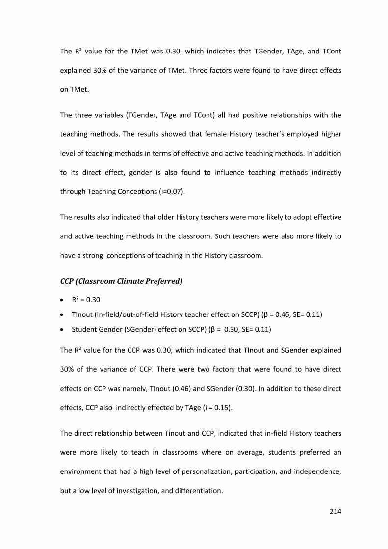
214

The R² value for the TMet was 0.30, which indicates that TGender, TAge, and TCont

explained 30% of the variance of TMet. Three factors were found to have direct effects

on TMet.

The three variables (TGender, TAge and TCont) all had positive relationships with the

teaching methods. The results showed that female History teacher’s employed higher

level of teaching methods in terms of effective and active teaching methods. In addition

to its direct effect, gender is also found to influence teaching methods indirectly

through Teaching Conceptions (i=0.07).

The results also indicated that older History teachers were more likely to adopt effective

and active teaching methods in the classroom. Such teachers were also more likely to

have a strong conceptions of teaching in the History classroom.

CCP (Classroom Climate Preferred)

R² = 0.30

TInout (In-field/out-of-field History teacher effect on SCCP) (β = 0.46, SE= 0.11)

Student Gender (SGender) effect on SCCP) (β = 0.30, SE= 0.11)

The R² value for the CCP was 0.30, which indicated that TInout and SGender explained

30% of the variance of CCP. There were two factors that were found to have direct

effects on CCP was namely, TInout (0.46) and SGender (0.30). In addition to these direct

effects, CCP also indirectly effected by TAge (i = 0.15).

The direct relationship between Tinout and CCP, indicated that in-field History teachers

were more likely to teach in classrooms where on average, students preferred an

environment that had a high level of personalization, participation, and independence,

but a low level of investigation, and differentiation.

215

The results also showed that classrooms which on average, had a higher proportion of

girls were more likely to prefer a higher level of personalisation (0.99), participation

(0.98), and investigation (0.80) but less investigation (-0.36), and differentiation (-0.92)

as their preferred classroom climate.

In relation to indirect effects, the path model (see Figure 7.1) showed classroom climate

preferred (CCP) was also influenced indirectly by teacher age (TAge) (0.15) through the

in-field/out-of-field construct. As mentioned earlier, older teachers, who are more likely

to be in-field History teachers, tended to have classes where students, on average,

wanted personalisation (0.99), participation (0.98), and investigation (0.80) as opposed

to independence (-0.36), and differentiation(-0.92) as their preferred classroom climate.

CCA (Classroom Climate Actual)

R² = 0.19

TInout (In-field/out-of-field History teacher effect on CCA) (β = -0.35, SE= 0.13)

Student Gender (SGender) effect on CCA) (β = 0.32, SE= 0.13)

The R² value for the CCA was 0.19, indicated that the model explained 19% of the

variance of CCA. There were two factors that were found to have direct effect on CCA

namely, a) TInout and b) Student Gender.

The results showed a negative relationship between TInout and CCA. This negative

association indicated that in-field History teachers were more likely to have classes in

which, on average, students experienced independence (-0.37), and differentiation

(-0.22) but less personalized, participatory and investigative activities, in their History

classroom. In contrast the results showed a positive relationship between SGender and

CCA. This result indicated that students’ in classrooms that had higher proportion of

216

girls were more likely to experienced more investigation (0.08), participation (0.94), and

personalisation (0.01) in their learning activities but less independence, and

differentiation compared to History classes that had more boys.

In addition to these direct effects, teacher age was found to have an indirect effect on

the actual classroom climate (CCA). The results revealed a significant negative

relationships betweenTAge (-0.12) and CCA through the in-field/out-of-field construct.

Older teachers, who were more likely to be in-field History teachers, tended to have

classes in which, on average, students in the actual History classroom were likely to

have experienced independence (-0.37), and differentiation (-0.22), but not

personalization, participation and investigation.

The Effect ON the variable in the Inner Model- Teacher Level Model 1

The section discusses variables in the inner model which had an effect on students’

approaches to learning as it was set up in Model 1, where all learning approaches were

combined into a single variable SLearning.

Student Approaches to Learning (SLearning)

R² = 0.41

Student Gender (SGender) effect on Learning (β = 0.34, SE= 0.12)

Student Ethnicity (SEthnic) effect on Learning (β = -0.47, SE= 0.09)

The R² value for the Learning was 0.41, which indicated that the model explained 41% of

the variance of students’ approaches to learning. Student gender (0.34) and SEthnic

were found to have direct effects on Learning. There were six manifest variables which

reflect students’ approaches to learning: (1) deep motive, (2) deep strategy, (3) surface

motive, (4) surface strategy, (5) achieving motive and (3) achieving strategy.

217

Results showed that on average, students in classrooms that had more girls and non-

Chinese students were more likely to adopt higher order learning approaches. (i.e.

Achieving or deep).

Students’ Perception of History Learning Objectives (SOutcome)

R² = 0.76

Student Approaches to Learning (SLearning) effect on Outcome (β = 0.84, SE= 0.05)

Teacher Year of Teaching (TExp) effect on Outcome (β = 0.18, SE= 0.08)

The R² value for the SOutcome was 0.76, indicating that the model explained 76% of the

variance of SOutcome. Two variables were found to have a direct effect on students’

perceptions of History learning objectives (SOutcome) namely, SLearning and teacher

year of Teaching (TExp). In addition to these direct effects SOutcome was also

influenced indirectly by TAge (i = 0.16), TInout (i = 0.02), SGender (i = 0.28) and SEthnic

(i = -0.40).

SLearning and TExp had positive effects on SOutcome. This result indicated that

students in the classes where, on average, employed deep and achieving approaches,

were more likely to have positive perceptions of History learning outcomes

(SOutcomes).

In addition, those students taught by experienced History teacher were more likely to

perceive that they had achieved the History learning outcomes.

218

Indirect Effects on students’ learning outcomes were evident in the case of the

following four factors:

Teacher Age (TAge) (i = 0.16) on Outcome

Teacher In-field/ out-of-field (TInout) (i = 0.02) on Outcome

Student Gender (SGender) (i = 0.28) on Outcome

Student Ethnicity (SEthnic) (i = -0.40) on Outcome

The results revealed positive effects of these variables, except for SEthnic (-0.40). Girls

as well students under older and in-field History teachers had stronger perceptions that

the History lessons have met their objectives compared to those Boys as well as

students under the out-of-field and younger History teachers.

SEthnicity variable (-0.40) had negative indirect effects on the students’ learning

outcomes in History learning. The results showed that non-Malay students such as

Chinese students’ were more less likely to perceived that History learning has met its

objectives.

The Effect ON the variable in the Inner Model- Teachers’ Level Model 2

This section discusses the variable in the inner model which had an effect on students’

approaches to learning as it was set up in Model 2. Only two of the students’

approaches to learning variables showed significant results. There were no significant

results on the Deep approach to learning.

SURFACE (Surface Learning Approaches)

R² = 0.24

Student Gender (SGender) effect on SURFACE (β = 0.39, SE= 0.17)

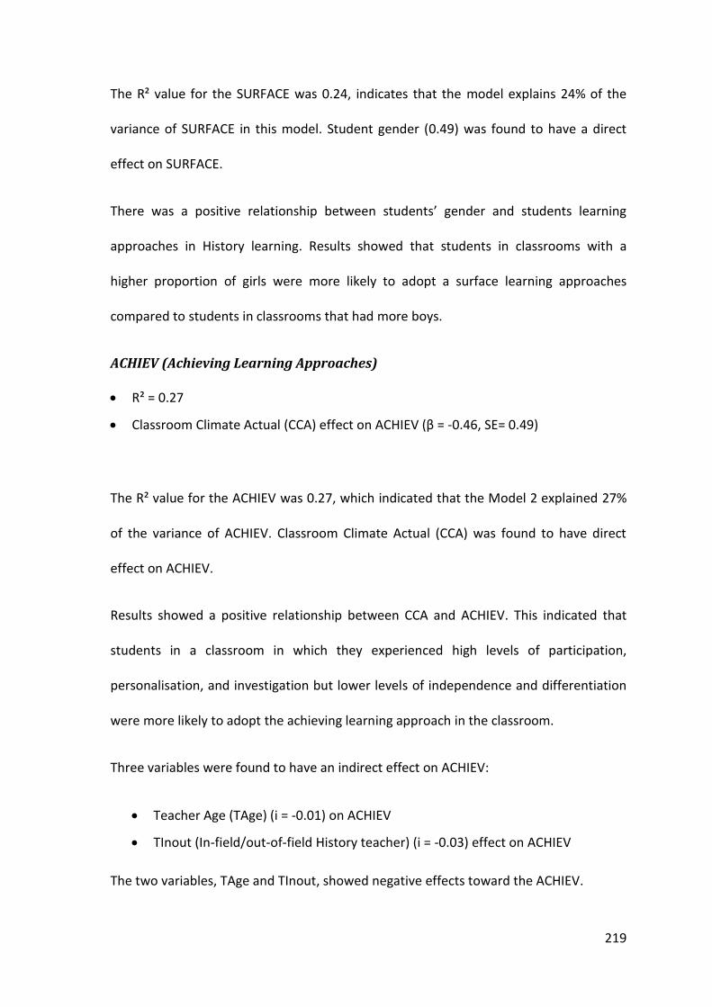
219

The R² value for the SURFACE was 0.24, indicates that the model explains 24% of the

variance of SURFACE in this model. Student gender (0.49) was found to have a direct

effect on SURFACE.

There was a positive relationship between students’ gender and students learning

approaches in History learning. Results showed that students in classrooms with a

higher proportion of girls were more likely to adopt a surface learning approaches

compared to students in classrooms that had more boys.

ACHIEV (Achieving Learning Approaches)

R² = 0.27

Classroom Climate Actual (CCA) effect on ACHIEV (β = -0.46, SE= 0.49)

The R² value for the ACHIEV was 0.27, which indicated that the Model 2 explained 27%

of the variance of ACHIEV. Classroom Climate Actual (CCA) was found to have direct

effect on ACHIEV.

Results showed a positive relationship between CCA and ACHIEV. This indicated that

students in a classroom in which they experienced high levels of participation,

personalisation, and investigation but lower levels of independence and differentiation

were more likely to adopt the achieving learning approach in the classroom.

Three variables were found to have an indirect effect on ACHIEV:

Teacher Age (TAge) (i = -0.01) on ACHIEV

TInout (In-field/out-of-field History teacher) (i = -0.03) effect on ACHIEV

The two variables, TAge and TInout, showed negative effects toward the ACHIEV.

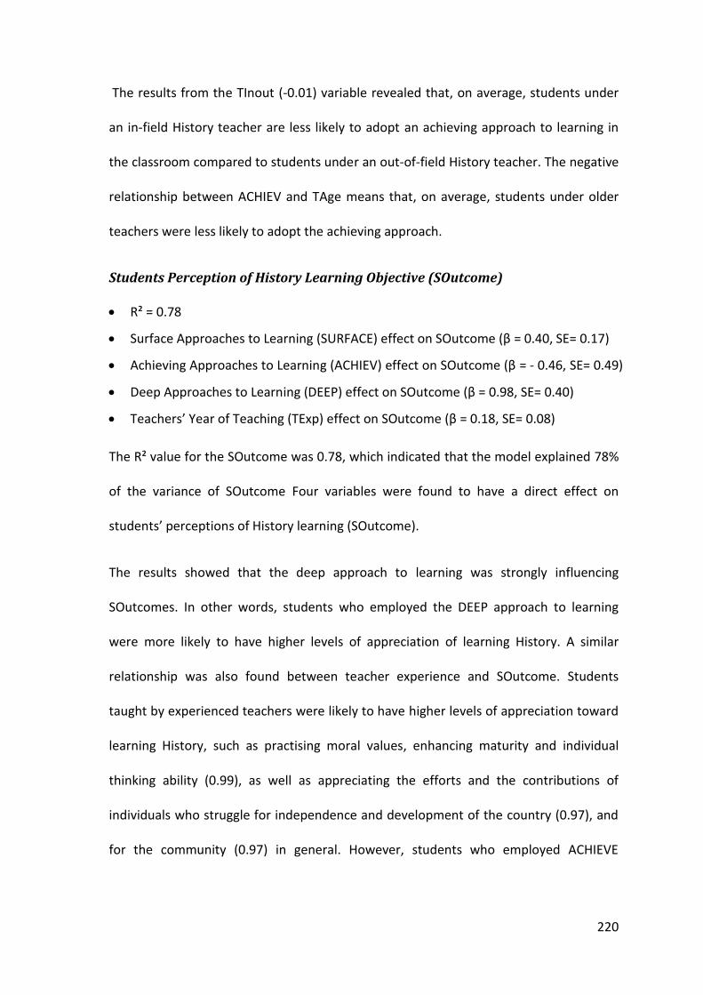
220

The results from the TInout (-0.01) variable revealed that, on average, students under

an in-field History teacher are less likely to adopt an achieving approach to learning in

the classroom compared to students under an out-of-field History teacher. The negative

relationship between ACHIEV and TAge means that, on average, students under older

teachers were less likely to adopt the achieving approach.

Students Perception of History Learning Objective (SOutcome)

R² = 0.78

Surface Approaches to Learning (SURFACE) effect on SOutcome (β = 0.40, SE= 0.17)

Achieving Approaches to Learning (ACHIEV) effect on SOutcome (β = - 0.46, SE= 0.49)

Deep Approaches to Learning (DEEP) effect on SOutcome (β = 0.98, SE= 0.40)

Teachers’ Year of Teaching (TExp) effect on SOutcome (β = 0.18, SE= 0.08)

The R² value for the SOutcome was 0.78, which indicated that the model explained 78%

of the variance of SOutcome Four variables were found to have a direct effect on

students’ perceptions of History learning (SOutcome).

The results showed that the deep approach to learning was strongly influencing

SOutcomes. In other words, students who employed the DEEP approach to learning

were more likely to have higher levels of appreciation of learning History. A similar

relationship was also found between teacher experience and SOutcome. Students

taught by experienced teachers were likely to have higher levels of appreciation toward

learning History, such as practising moral values, enhancing maturity and individual

thinking ability (0.99), as well as appreciating the efforts and the contributions of

individuals who struggle for independence and development of the country (0.97), and

for the community (0.97) in general. However, students who employed ACHIEVE

221

approach to learning showed to lower levels of appreciation of the learning History

objectives in terms of individual, country and community.

The results indicated that the students’ view of History learning (SOutcome) was

indirectly influenced by three factors

Teacher Age (TAge) (i = 0.16)

Teacher In-field/ out-of-field (TInout) (i = 0.03)

(SGender) (i = 0.12)

Classroom Climate Actual (CCA) (i = -0.24)

Teachers’ age and qualifications have indirect effects on the students’ perceptions of

History learning (SOUTCOME). Girls as well as students under older teachers, who were

the in-field History teachers, were more likely to perceive that the History lesson have

met their objectives of learning History such as practising moral values, and enhancing

maturity and the thinking ability individuals (0.99), as appreciating the efforts and the

contributions of individuals who struggled for independence and development of the

country (0.97) and community (0.99), compared to boys and students under the

younger out-of-field History teachers.

CCA (-0.24) had an indirect negative effect on SOutcome. The result indicated that

students who experienced participation, personalisation and innovation in their

classroom were more likely to perceive that the objectives of learning History had been

achieved.

222

7.6 Summary of Analysis Teachers’ Level Path– Models 1 and 2

There were two teachers’ level path models which were examined in this chapter. In the

first model (Model 1) students’ learning approaches were combined into a single

variable as ‘SLearning’ (refer to Figure 7.1) In the second model (Model 2) the Learning

Approache variables were discussed as six separate variables surface motive, deep

motive, achieving motive, surface strategy, deep strategy, achieving strategy (refer to

Figure 7.2). Apart from this one variation the 2 path models had identical variables.

In this research PLSPATH analysis was carried out to investigate the possible

relationships which could help to answer the three major research questions as

advanced in Chapter 2. These relationships were between teachers’ characteristics (age,

gender, ethnicity, teacher in-field and out-of-field, and teacher experience), teaching

conception, teacher approaches, teaching methods, and students’ characteristics (age,

gender, ethnicity), classroom environment (Preferred and Actual), approaches to

learning (Surface, Achieving and Deep) and students’ perceptions of History learning

outcomes in the classroom. The main relationships revealed in the PLSPATH analyses

are discussed below.

(a) For Conceptions of teaching, the results indicated that teacher gender had a positive

relationship with teaching conceptions. This result meant that female History teachers

had higher teaching conceptions compared to the male History teachers.

(b) In the case of Teaching approaches to teaching, the results revealed that there was a

positive relationship between Teaching conceptions and Teaching approaches This

meant that those History teachers who had higher teaching conceptions were more

223

likely to employ both teaching approaches information transfer or teacher-focused and

conceptual change or student-focused. The analysis also revealed that female teachers

who in general, had stronger teaching conceptions also had stronger teaching

approaches.

(c) In relation to Teaching methods, the results showed positive relationships with

teaching conceptions and teaching approaches, as well as gender and age. The results

showed that female History teachers were more likely to employ higher level of

teaching methods in terms of being both effective and active. The results also indicated

that as their age increased History teachers were more likely to adopt effective and

active teaching methods in the classroom. In other words, older female teachers were

more likely to apply higher levels of teaching conceptions in the History classroom.

(d) For Teaching experience (years of teaching), the results indicated a positive

relationship with two variables, teachers’ age and teacher TInout (‘in-field’ and ‘out-of-

field’) History teachers. This meant that the more experienced teachers were more

likely to be older and to be in-field History teachers than their younger counterparts.

(e) Preferred Classroom Climate had a positive relationship with teacher TInout (‘in-field’

and ‘out-of-field’) History teachers and students’ gender. These results indicated that

students under in-field History teachers, or in a class with a high proportion of girls were

more likely to prefer an environment that had higher levels of personalization,

participation, and independence, but lower levels of investigation, and differentiation.

(f) Classroom Climate Actual had a negative relationship on teacher TInout, while having

a positive relationship with the students’ gender. The negative association indicated

224

that in-field History teacher were more likely to have classes in which, on average,

students were likely to experience more independent, participative, and differentiative

activities but less personalized, and investigative activities, in their History classroom.

However, this result is in contrast, to the negative relationship between student gender

and Classroom Climate Actual.

(g) For Student Approaches to Learning, the results showed that on average, students in

classrooms that had more girls were more likely to adopt high order learning

approaches. There was also a negative relationship between Student Ethnicity and

Learning. The implications were that Malay (D) students were more likely to adopt high

order learning approaches followed by Other ethnic, Indian, and Chinese backgrounds.

(h) With Surface Learning Approaches, the results indicated a positive relationship with

student gender. Classrooms with a high proportion of girls were more likely to adopt

surface learning approaches, compared to students in classrooms that had more boys.

(i) Achieving Learning Approaches had a positive relationship with Actual classroom

climate. This result indicated that when students were in the classroom in which they

have higher levels of participation, personalisation, and investigation but lower level of

independent and differentiation, they were more likely to adopt achieving learning

approaches in the classroom.

(j) Students, Perceptions of History learning (SOutcomes), showed a positive

relationship with surface and deep approaches, to learning and also with the teacher

experience. However, there was a negative relationship with achieving approaches. The

result indicated that students in classroom in which a high proportion employed of DEEP

225

approach to learning were more likely to appreciate the objectives of learning History.

In addition, students taught by experienced teacher were likely to perceive the

objectives of learning History. However, students who employed achieving approach to

learning were less likely to appreciate the objectives of learning History in the classroom.

In relation to the focus of this study investigation, the differences between out-of-field

and in-field teachers in History classrooms in Kuala Lumpur, the path analysis showed

an indirect relationship between Teachers’ qualification and students’ learning

outcomes through the variables of Teachers Experience. However, one of the most

important findings in both Path Analysis Models was the absence of any direct

relationship between the teacher qualification variables (out-of-field/ in-field) and

Students’ History learning outcomes. The implications of this finding are considered in

Chapter 10. The following chapter reports the results of the PLSPATH analysis of the

student level data.

226

Chapter 8 Partial Least Squares Path

Analysis: Student Level ________________________________________________________________________

8.1 Introduction

This chapter discusses the results of the Partial Least Squares Path (PLSPATH) analysis at

the students level. The partial least squares path analysis (PLSPATH) program Version

3.01 (Sellin, 1989) was carried out in this study based on the students’ data set (1653

students, Year 11). The relationships that have been investigated in this chapter were

similar to the previous chapter, which used PLSPATH analysis of teachers’ data. The

variables investigated were teachers’ characteristics (age, gender, ethnicity, teacher in-

field and out-of-field, and teacher experience), teacher conceptions, teacher

approaches, teaching methods, and students’ characteristics (age, gender, ethnicity),

classroom climate preferred, classroom climate actual, approaches to learning (Surface,

Achieving and Deep approaches), and students’ perceptions of History learning

(Outcomes) in the classroom. However, this analysis is concerned about the processes

occured at the student level.

8.2 Model Building in the PLSPATH analyses

In this chapter, as in Chapter 7, two path models were developed in order to explore the

students’ level data. In Path Model 1, the latent construct of ‘Learning Approaches,’

which was reflected by six components, such as surface motive and surface strategy,

deep motive and deep strategy, as well as achieving motive and achieving strategy, was

represented by a variable given the acronym ‘SLearning’. On the other hand, in students,

227

Level Path Model 2, the three components of ‘ Learning Approaches’ were consider as

separate latent variables, labelled as ‘Surface’, ‘Achieving’ and ‘Deep’. Each of these

learning approaches was reflected by two manifest variables, labelled as motive and

strategy. The other variables in the two Students’ Level Path Models were the same. In

particular, the outcome variables was the same in both students’ Level Path Models:

Students’ perceptions of the achievement of the History Learning Objectives, which was

given the acronym ‘SOUTCOME’

AMOS 17 (Arbuckle, 2008) was used to draw the PATH diagrams using the path

coefficients based on the PLSPATH results. There were 15 and 17 LVs included in Models

1 and 2 respectively. Overall, there 42 MVs in each of the models. Tables 8.1 and 8.2

exhibit all the variables in Models 1 and 2 that were proposed in this study. The latent

variables (LVs) and manifest variables (MVs) are also listed in Table 8.1 and 8.2

according to their acronyms, together with a description of each variable. In addition,

the mode of each block, such as unity, inward or outward, is presented.

The interrelationships among the variables in the Student’ Level Path Models 1 and 2

are shown in two path diagrams, Figures 8.1 and 8.2 respectively. A path diagram

consists of two models; the inner model and the outer model. The inner model, on one

hand, consists of relationships among LVs. The outer model, on the other hand, shows

the relationships between each LV and its corresponding MVs. Overall, there are 42

MVs in each of the models. There are two types of LVs, namely 1) exogenous

(independent) or antecedent variables, which receive no causal input from other

variables; and 2) endogenous (dependent) variables, which receive one or more causal

inputs from other variables. In Models 1 and 2 the exogenous (independent) variables

228

at the student level are teachers’ characteristics such as age, gender, ethnicity, years of

teaching experience), and in-field or out-of-field History qualifications, as well students’

characteristics such as age, gender, and ethnicity. The endogenous (dependent)

variables at the teacher level are teaching approaches, teaching methods and teaching

conceptions and for the student level are classroom environment (actual and preferred),

learning approaches (Surface, Deep and Achieving).The criterion variable was students’

learning History objective (country, community, and individual).

Figures 8.1, Figure 8.2, Figure 8.3 and 8.4 display all the variables involved in these

Student Level Path Models. The manifest variables are presented in box shapes while

the latent variables are shown as oval shapes. The diagrams present the relations

between the teacher and student teaching and learning History in the classroom

variables at the students’ level. The reports on the relationships are discussed in two

part, as they related to the outer (measurement) model, and the inner (structural)

model.

The full list of the variables in this study is presented in Tables 8.1 and Table 8.2 in

relation to the two Hypothesised Models 1 and 2 labelled Figures 8.1 and 8.2; and the

Final Models labelled 1 and 2 as presented in Figures 8.2 and 8.4.

229

Table 8. 1 Variables in the Student Level Path Model 1



Description Coding



TEthnic Inward Teacher’s ethnicity TMalay Malay (Dummy) 0=Not Malay 1=Malay

TChinese Chinese 0=Not Chinese 1=Chinese TIndian Indian 0=Not Indian 1=Indian TOther Iban/Melanau/Thai 0=Not Other 1=Other TInout unity Teacher's qualification In-field In-field/ out of-field 0=Out of-field 1=In-field TExp unity Teacher Years of teaching Tytea Teaching experience



TMet outward Teaching Methods TEft Teaching Effective Factor Scores TAct Teaching Active Factor Scores





SAge unity Student’s age SYear Age in years 17-18

SGender unity Student’s gender SGdr 0=Male 1= Female 0=M 1=F SEthnic Inward Student’s ethnicity TMalay Malay (Dummy) 0=Not Malay 1=Malay

TChinese Chinese 0=Not Chinese 1=Chinese TIndian Indian 0=Not Indian 1=Indian TOther Iban/Melanau/Thai 0=Not Other 1=Other SCCA outward Classroom Climate Actual Spar Participation Factor Scores Sind Independence Factor Scores




SCCP outward Classroom Climate Preferred SINV Investigation Factor Scores

SPER Personalisation Factor Scores




SLearning outward Student’s Approaches to Learning

SSM Surface Motive Factor Scores

SSS Surface Strategy Factor Scores

SAM Achieving Motive Factor Scores

SAS Achieving Strategy Factor Scores

SDM Deep Motive Factor Scores

SDS Deep Strategy Factor Scores


SCountry Appreciating country Factor Scores



Factor Scores

230

Figure 8. 1 Hypothesised Model For Students’ Level Model 1

231

TMet

TExp

TGender

TEthnic

TInout

TCont

SEthnic

CCA

SGdr CCP

Learning

Outcome

TEft TAct SGDR

SSM

SSS

SAM

SCountry

SCommu

SIndivid

SPar0.86

SInd-0.5

SPer0.64

SInv0.75

SDfr-0.57OtherIndianChineseMalay

TExam

0.9

TKDeli0.92

TAttPro

0.81

TAbi

0.93

Condanc

0.91

Other

Indian

Chinese

Malay

SINV

0.69


-0.2

SDIFFER

TAge

TGdr

TAge

Infield

Tyrtea1

TAppTConChan

TInfoTra 0.92

1

SAS

SDM

SDS

10.93 -0.88

0.98

.26(.02)

.35(.00)

.14(.01)

.31(.04)

.08(.02)

.28(-.00)

.17(.02)

.09(.02)

-.26(.03)

-.22(.02)

.05(.02) -.15(.02).08(.02)

.59(.03).14(02)

.11(.03)

SAge

SAge

-.12(.02)

0

0.38

0.85

0.16-0.11 0.04

.12(.02)

0.990

.29(.04)

.06(.02)

.18(.03)

1

.15(.05)

.22(.02)

-.05(-.02)

1

.90(-.01) .14(.02)

0.930.97

.08(.03)

1

0.980.97

0.96

0.71-0.070.96

0.94

0.96

0.94

.33(.03)

0.95

Figure 8. 2 Final Model for Students’ Level Model 1

232

Table 8. 2 Variables in the Student Level Path Model 2



Description Coding



TEthnic Inward Teacher’s ethnicity TMalay Malay (Dummy) 0=Not Malay 1=Malay

TChinese Chinese 0=Not Chinese 1=Chinese

TIndian Indian 0=Not Indian 1=Indian

TOther Iban/Melanau/Thai 0=Not Other 1=Other

TInout unity Respondent’s qualification In-field In-field/ out of-field In-field/ out of-field TExp unity Years of teaching Tytea Teaching experience



TMet outward Teaching Methods TEft Teaching Effective Factor Scores TAct Teaching Active Factor Scores





SAge unity Student’s age TYear Age in years 17-18

SGender unity Student’s gender SGdr 0=Male 1= Female 0=M 1=F

SEthnic Inward Student’s ethnicity TMalay Malay (Dummy) 0=Not Malay 1=Malay

TChinese Chinese 0=Not Chinese 1=Chinese

TIndian Indian 0=Not Indian 1=Indian

TOther Iban/Melanau/Thai 0=Not Other 1=Other

SCCA outward Classroom Climate Actual SPar Participation Factor Scores Sind Independence Factor Scores




SCCP outward Classroom Climate Preferred SINV Investigation Factor Scores SPER Personalisation Factor Scores




SSurface outward Surface Approaches SSM Surface Motive Factor Scores SSS Surface Strategy Factor Scores

SDeep outward Deep Approaches SAM Achieving Motive Factor Scores SAS Achieving Strategy Factor Scores

SAchieving outward Achieving Approaches SDM Deep Motive Factor Scores SDS Deep Strategy Factor Scores


SCountry Appreciating country

Factor Scores



Factor Scores

233

Figure 8. 3 Hypothesised Model for Students’ Level Model 2

234

TMet

TExp

TGender

TEthnic

TInout

TCont

SEthnic

CCA

SGdrCCP

Deep

Outcome

TEft TAct

SGDR

SSM

SSSSAM

SCountry

SCommu

SIndivid

SPar0.36

SInd0.5

SPer0.64

SInv0.75

SDfr-0.57

OtherIndianChineseMalay

TExam

0.9

TKDeli

0.92

TAttProTAbi

0.93

Condanc

0.91

Other

Indian

Chinese

Malay

SINV

0.69


-0.2

SDIFFER

TAge

TGdr1

TAge1

Infield

Tyrtea1

TApp

TConChan 0.95

TInfoTra 0.92

1

SAS

SDM

SDS

10.93 -0.88

0.98

.08(.03)

-.26(.02)

.35(.00)

Surface

Achieving

.20(.01)

.01(.00)

.16(.02)

0.04

0

0.38

0.85

0.14

0.970.93

0.990.37

0.960.95

0.990.99

0.970.98

0.96

.51(.03)

.14(.02)

.15(.05)

.28(.03)

.11(.02)

.28(-.00)

.16.02)

.90(-.01)

0

-0.110. 99

0.81

.14(.02)

.14(.01)

.08(.02)

.31(.04)

.22(.02)

.18(.02)

.29(.04)

.09(.02).25(.02)

.06(.02)

.11(.03)

.72(-.00)

.93(-.00)

-.05(-02)

.17(.02)

05.(.02)

.23(.02)

Figure 8. 4 Final Model for Students’ Level Model 2

235

Table 8. 3 Indices for the Outer Model - Students’ Level Path Model 1 and 2

MODEL 1 MODEL 2

Variables Mode W L C R T W L C R T

AGE/years unity 1 1 1 0 0 1 1 1 0 0

GENDER/sex unity 1 1 1 0 0 1 1 1 0 0

TEthnic inward

Malay (D) 0 0 0 0 0 0 0 0 0 0

Chinese 0.49 0.38 0.14 0 0.02 0.49 0.38 0.14 0 0.02

Indian 0.91 0.85 0.72 0 0.01 0.91 0.85 0.72 0 0.01

Other 0.26 0.14 0.02 0 0.01 0.26 0.14 0.02 0 0.01

TInout unity 1 1 1 0 0 1 1 1 0 0

TExp/ Tyrteac unity 1 1 1 0 0 1 1 1 0 0

TApp outward

TInfoTra 0.48 0.92 0.86 0.09 0.58 0.48 0.92 0.86 0.09 0.58

TConChan 0.58 0.95 0.90 0.09 0.58 0.58 0.95 0.90 0.09 0.58

TMet outward

TEft 0.61 0.97 0.93 0.37 0.64 0.61 0.97 0.93 0.37 0.64

TAct 0.44 0.93 0.90 0.35 0.64 0.44 0.93 0.90 0.35 0.64

TCont outward

TExam 0.24 0.90 0.82 0.11 0.77 0.24 0.90 0.82 0.11 0.77

TKDeli 0.23 0.92 0.87 0.11 0.80 0.23 0.92 0.87 0.11 0.80

TAttPro 0.13 0.81 0.66 0.09 0.66 0.13 0.81 0.66 0.09 0.66

TAbiDev 0.22 0.93 0.84 0.11 0.77 0.22 0.93 0.84 0.11 0.77

ConDance 0.28 0.91 0.80 0.11 0.69 0.28 0.91 0.80 0.11 0.69

Sage/ years unity 1 1 1 0 0 1 1 1 0 0

SGender /sex unity 1 1 1 0 0 1 1 1 0 0

SEthnic inward

Malay (D) 0 0 0 0 0 0 0 0 0 0

Chinese 1.01 0.99 0.98 0.00 0.37 1.01 0.99 0.98 0.00 0.37

Indian 0.06 -0.11 0.01 0.00 0.03 0.06 -0.11 0.01 0.00 0.03

Other 0.14 0.04 0.00 0.00 0.01 0.14 0.04 0.00 0.00 0.01

SCCA outward

SPar 0.38 0.86 0.74 0.08 0.55 0.38 0.86 0.74 0.08 0.55

Sind -0.14 -0.50 0.25 0.03 0.39 -0.14 -0.50 0.25 0.03 0.39

SPer 0.40 0.64 0.41 0.04 0.16 0.40 0.64 0.41 0.04 0.16

SInv 0.26 0.75 0.56 0.06 0.57 0.26 0.75 0.56 0.06 0.57

SDfr -0.26 -0.57 0.32 0.03 0.15 -0.26 -0.57 0.32 0.03 0.15

SCCP outward

SINV 0.15 0.69 0.47 0.04 0.78 0.15 0.69 0.47 0.04 0.78

SPER 0.33 0.98 0.95 0.08 0.97 0.33 0.98 0.95 0.08 0.97

SPARTICI 0.29 0.93 0.88 0.07 0.97 0.29 0.93 0.88 0.07 0.97

SINDEPEN -0.24 -0.20 0.04 0.00 0.46 -0.24 -0.20 0.04 0.00 0.46

SDIFFER -0.30 -0.88 0.77 0.06 0.73 -0.30 -0.88 0.77 0.06 0.73

SOutcome outward

SCountry 0.34 0.98 0.96 0.10 0.91 0.34 0.98 0.96 0.10 0.91

SCommunity 0.34 0.97 0.94 0.45 0.88 0.34 0.97 0.94 0.45 0.88

SIndividual 0.35 0.96 0.95 0.45 0.89 0.35 0.96 0.95 0.45 0.89

SLearning

SSM 0.18 0.73 0.55 0.12 0.96

SSS -0.01 -0.01 0.00 0.00 0.82

SAM 0.24 0.96 0.92 0.10 0.97

SAS 0.22 0.94 0.88 0.19 0.99

SDM 0.24 0.96 0.92 0.20 0.99

SDS 0.22 0.94 0.88 0.20 0.99

Surface outward

SSM 1.10 0.99 0.99 0.10 0.22

SSS -0.13 0.37 0.14 0.01 0.22

Achiev outward

SAM 0.55 0.96 0.92 0.59 0.67

SAS 0.50 0.95 0.90 0.58 0.67

Deep outward

SDM 0.52 0.99 0.97 0.87 0.89

SDS 0.50 0.99 0.97 0.87 0.89

Notes: W =Weight, L= Loadings, C= communality, R= Redundancy and T= Tolerance

236

8.3 Outer Model –Students’ Level Path Model 1and 2

The outer model results indicate the strength of the relationships between the latent

variables and the manifest variables, either in forming or reflecting the latent variables

concerned (Rintaningrum et al., 2009). In PLSPATH, ‘PATTERN’ is the command line that

refers to the relationship between LV and MV variables. In this model there were three

modes involved: formative, reflective and unity mode (Darmawan, 2003, Rintaningrum

et al., 2009). To refine the outer model, those variables which have no meaningful or

adequate influence on the formation or reflection of the LVs, need to be removed from

further analysis. The deletion procedure is based on five indices, namely, weight,

loading, communality, redundancy, and tolerance. Additionally, due to the limitations in

PLSPATH, Sellin (1989) suggested using jackknife methods to overcome the lack of any

test of significance in PLSPATH analysis. This method, calculates the estimation of the

standard error to use as a test of the significance of the results.

Table 8.3 presents the fit indices for the Students’ Level Path Models 1 and 2. The

following discussion of both these models is based on the five indices weight, loading,

communality, redundancy, and tolerance. The weight indices are the strength of the

regression relationships between LVs and MVs in the inward or formative mode.

Relationships between LVs and MVs are considered meaningful if the values of the

associated weight are equal to or greater than 0.10 (Sellin & Keeves, 1997). Where a

weight of zero is recorded, the MV acts as a reference in the use of a dummy for

variable regression analysis. In this study there were two inward mode variables,

namely TEthnic and SEthnic.

237

Another criteria used for the outer model indices is loading, which indicates the

strength of the factor analytic relationship between MVs and LVs in the outward or

reflective mode (Sellin and Keeves, 1997). There are seven blocks with outward

(reflective) modes in this model. Values equal to or larger than 0.40 are considered

adequate loading values (Sellin and Keeves, 1997).

Communality indicates the strength of the outer model and is calculated as the squared

correlation between MVs and their associated latent variables (Sellin, 1989. Falk 1987)

claimed that the strength of the outer model is measured by the average communality

values of all the variables He added that, communality values greater than 0.30, were

considered strong. The higher the average for this communality index, the better the

outer model (Falk, 1987).

Redundancy indicates the “joint predictive power of inner model and outer

relationships as estimated for a given data set” (Sellin, 1989). Tolerance indicates the

possible multicollinearity within a corresponding block of MVs. Tolerance is calculated

as the squared correlation between a given MV and the remaining MVs belonging to the

same LV (Sellin, 1995). It is commonly accepted (Sellin, 1989) that if the tolerance value

is 0.50 or higher, multicollinearity within a block of MVs can be considered adequate

According to Darmawan (2003), tolerance indicates the possibility of seriously damaging

multicollinearity within the corresponding blocks of MVs. However these effects are

considered damaging to the inward (formative) mode, rather than to the outward

(reflective) mode. In this recent study, the possible multicollinearity in the model was

strong in most the outward variables expect for the inward variables.

238

Discussion - Outer Models: Student Level Path Model 1 and 2

This section discusses the path model at student level Models 1 and 2. The distinction

between student level model 1 and model 2 was the ‘Learning Approaches’ variables.

On one hand, in Model 1, all variables were combined as student learning approaches

‘SLearning’. On the other hand, in Model 2, the ‘Learning Approaches’ variables were

discussed separately as such: surface, deep, and achieving. The results of the PLSPATH

analysis of the student level data are discussed in two parts: a) outer (measurement)

model and b) the inner (structural) model. This following section considers the former in

relation to Student Level Path Models 1 and 2 (see Table 8.3)

Teachers Age (TAge)

Teachers’ age (TAge) as a latent variable was formed by a single manifest variable,

namely TYear. In the model, the TYear variable was reflected by a single indicator and


Teachers’ Gender (TGender)

Teachers’ Gender (TGender) was also reflected by a single indicator namely, TGdr. The


Teacher Qualifications (Tinout)

Teacher Qualification, in relation to in-field and out-of-field teachers (Tinout) was also

reflected by a single indicator namely, TIn-field. The value of its loading was 1.00 (unity).

Teachers’ Experience (TExp)

Teachers experience (TExp) was also reflected by a single indicator namely, Tytea. The


239

Student Age (SAge)

Student age (SAge) as a latent variable was formed out of a single manifest variable,

namely SAge. In the model, the SAge variable was reflected by a single indicator and the


Students Gender (SGender)

Students’ Gender (SGender) was also reflected by a single indicator namely, SGdr. The


Students’ Ethnicity (SEthnic)

Student Ethnic (SEthnic) was formed by four MVs that represented the four ethnic

groups the students belonged to, namely Malay, Chinese, Indian and Other Ethnicities.

In this model, the Malay group was used as a reference point (Dummy). Therefore, the

factor weight for Malay was set to 0. The factor weights for the three other groups were

0.99, -0.11 and 0.04, for Chinese, Indian, and Other Ethnicities respectively.

Teachers’ Ethnicity (TEthnic)

Teachers’ Ethnicity (TEthnic) was formed by four MVs that represented the four ethnic

groups the teachers could belong to, namely Malay, Chinese, Indian and Other

Ethnicities. In this model, the Malay group was used as a reference point (Dummy).

Therefore, the factor weight for Malay was set to 0. The factor weights for the three

other groups were 0.38, 0.85 and 0.14, for Chinese, Indian, and Other Ethnicities

respectively.

Teacher Approaches (TApp)

Teacher Approaches (TApp) as a latent variable was reflected by only two MVs, namely,

information transfer/teacher-focused (TInfoTra) and conceptual change/student-

240

focused (TConChan). As an outward latent constructs, TApp was strongly reflected by

these two MVs, with factor loadings of 0.92 and 0.95.


Teaching Methods (TMet) construct was also reflected by two MVs namely, effective

teaching (TEft) and active teaching (TAct). These two MVs were composite scores

calculated using a principal component method. The way in which these MVs were

formed explained in Chapter 5. These two MVs had high loadings (0.97 and 0.93), which

indicated that this construct was strongly reflected by the two MVs.

Teacher Conceptions (TCont)

Five MVs reflected the construct of Teacher Conceptions (TCont), namely Exam

preparation (TExam), Knowledge delivery (TKDeli), Attitude promotion (TAttPro), Ability

development (TAbiDev) and Conduct guidance (ConDance). The sizes of the factor

loading were moderate to high, being 0.90, 0.92, 0.81, 0.93 and 0.91respectively. These

results indicated that all MVs were strong reflectors of the construct.

Students Classroom Climate Actual (SCCA)

Students Classroom Climate Actual (SCCA) was an outward latent variable reflected by

five MVs, namely Student Participation (Spar), Student Independence (Sind), Student

Personalisation (SPer), Student Investigation (SInv) and Student Differentiation (SDfr).

The factor loadings for SPar, SInd, SPer, SInv, and SDfr were 0.86, -0.50, 0.64, 0.75 and -

0.57. These coefficients indicated that the SCCA was strongly reflected by Student

Participation (Spar), Student Personalisation (SPer), and Student Investigation (SInv).

Participation was found to be the strongest reflector of SCCA in Malaysian context.

Furthermore, Investigation and Differentiation both had negative coefficients, which

241

could be interpreted that those classes where students actually experienced high levels

of participation, personalisation and investigation scored low on independence and

differentiation. The negative loadings indicated the corresponding manifest variables

were in the opposite direction on the scale to those MVs that had positive loadings.

Students’ Classroom Climate Preferred (SCCP)

In a similar way to Classroom Climate Actual, Students’ Classroom Climate Preferred

(SCCP) was reflected by five MVs, namely, Student Investigation (SINV), Student

Personalisation (SPER), Student Participation (SPARTICI), Student Independence

(SINDEPEN), and Student Differentiation (SDIFFER). The factor loadings were strong for

SINV, SPER and SPARTICI (0.69, 0.98, and 0.93), with the exception of the negative

loadings for SINDEPEN (-0.20) and SDIFFER (-0.88). This result could be interpreted that

students in those classes that preferred Investigation, Personalisation, and Participation

would score low on Independence and Differentiation. The negative loadings indicated

that the corresponding manifest variables were in the opposite direction on the scale

compared to those MVs that had positive loadings.

Students’ Learning Outcomes (SOutcome)

Students’ Learning Outcomes (SOutcome) were reflected by Student Country (SCountry),

Student Community (StudentCommunity), and Student Individual (SIndividual). These

three MVs had high factor loadings of 0.98, 0.97, and 0.96 respectively. This result

indicated that this construct was strongly reflected by the three MVs.

Student Learning (SLearning)

Students’ Learning (SLearning) was an outward mode latent variable reflected by six

MVs, namely Student Surface Motive (SSM), Student Surface Strategy (SSS),Student

242

Achieving Motive (SAM), Student Achieving Strategy (SAS), Student Deep Motive (SDM),

Student Deep Strategy (SDS). All MVs were strong reflectors of the construct, with

loadings ranging from 0.37 to 0.99. SDM and SDS were found to be the strongest

reflector of this construct. This construct was only available in the Model 1.

SURFACE

SURFACE was reflected by only two manifest variables namely, Student Surface Motive

(SSM) and Student Surface Motive (SSM). As an outward latent construct, SURFACE was

reflected by these two MVs with the factor loadings of 0.99 and 0.37 respectively. This

construct is only in Model 2.

ACHIEVING (Achiev)

In a similar way to SURFACE, ACHIEVING (Achiev) was also reflected by two MVs namely,

Student Achieving Motive (SAM) and Student Achieving Strategy (SAS). Both MVs were

strong reflectors of achieving, with factor loadings of 0.96 and 0.95. This construct was

only in Model 2.

DEEP

DEEP was reflected by only two MVs variables namely, Student Deep Motive (SDM),

anad Student Deep Strategy (SDS). As an outward latent construct, DEEP was strongly

reflected by these two MVs, with factor loadings of 0.99 and 0.99. This construct was

only in Model 2.

243

Table 8. 4 Path Indices for PLS Inner Model – Student’ Level Path Model 1 and 2

MODEL 1 MODEL 2 Variable

Beta JknMean JknStd Corr Tolerance Beta JknMean JknStd Corr Tolerance

Teacher in-field/out-of field (TINOUT) Teacher Age (TAGE) 0.82 0.82 0.03 0.19 0.17 0.82 0.82 0.03 0.19 0.17 Teacher Ethnicity (TETHNIC) 0.26 0.26 0.02 0.30 0.17 0.26 0.26 0.02 0.30 0.17

Teaching Conception (TCONCEPT) Teacher Gender (TGENDER) 0.35 0.35 0.00 0.34 0.00 0.35 0.35 0.00 0.34 0.00 Teacher Age (TAGE) 0.14 0.14 0.01 0.12 0.00 0.14 0.14 0.01 0.12 0.00

Teacher Approaches (TAPPROAC) Teacher Conception (TCONCEPT) 0.35 0.35 0.00 0.31 0.00 0.35 0.35 0.00 0.31 0.00 Teacher Age (TAGE) 0.08 0.08 0.01 0.06 0.00 0.08 0.08 0.01 0.06 0.00

Teaching Method (TMETHOD) Teacher Gender (TGENDER) 0.18 0.18 0.03 0.33 0.13 0.18 0.18 0.03 0.33 0.13 Teacher Conception (TCONCEPT) 0.28 0.28 -0.00 0.52 0.56 0.28 0.28 -0.00 0.52 0.56 Teacher Approaches (TAPPROAC) 0.22 0.22 0.02 0.49 0.53 0.22 0.22 0.02 0.49 0.53 Teacher Year of Teaching (TEXP) 0.29 0.29 0.04 0.32 0.02 0.29 0.29 0.04 0.32 0.02

Teacher Year of Teaching (TEXP) Teacher Age (TAGE) 0.89 0.89 -0.01 0.92 0.04 0.89 0.89 -0.01 0.92 0.04 Teacher in-field/out-of field (TINOUT) 0.14 0.14 0.02 0.31 0.04 0.14 0.14 0.02 0.31 0.04

Classroom Climate Preferred (CCP) Teacher Gender (TGENDER) -0.05 -0.05 -0.02 -0.06 0.00 Teacher in-field/out-of field (TINOUT) 0.14 0.14 0.02 0.19 0.10 0.14 0.14 0.02 0.19 0.10 Student Gender (SGENDER) 0.11 0.11 0.03 0.12 0.00 0.11 0.11 0.03 0.12 0.00 Student Age (SAGE) -0.12 -0.12 0.02 -0.11 0.01 Teacher Year of Teaching (TEXP) 0.15 0.15 0.05 0.20 0.10 0.14 0.14 0.03 0.20 0.10

Classroom Climate Actual (CCA) Teacher Ethnicity (TETHNIC) 0.17 0.17 0.02 0.17 0.14 Teacher in-field/out-of field (TINOUT) 0.09 0.09 0.02 0.06 0.10 0.09 0.09 0.02 0.17 0.02 Student Ethnicity (SETHNIC) -0.26 -0.26 0.03 -0.25 0.03 0.26 0.26 0.03 -0.25 0.03 Teaching Method (TMETHOD) 0.06 0.06 0.02 0.13 0.10 0.06 0.06 0.02 0.13 0.02

Student Approaches to Learning (LEARNING) Student Gender (SGENDER) 0.12 0.12 0.02 0.14 0.00 Student Ethnicity (SETHNIC) -0.22 -0.22 0.02 -0.31 0.10 Classroom Climate Actual (CCA) 0.33 0.33 0.03 0.39 0.10

Students’ Perception of History Learning (SOUTCOME)

Teacher in-field/out-of field (TINOUT) 0.05 0.05 0.02 0.03 0.02 Student Ethnicity (SETHNIC) -0.15 -0.15 0.02 -0.34 0.13 Classroom Climate Actual (CCA) 0.08 0.08 0.02 0.35 0.18 0.11 0.11 0.02 0.37 0.17 Student Learning Approaches (LEARNING) 0.59 0.59 0.03 0.66 0.20 Surface Learning Approaches (SURFACE) 0.16 0.16 0.02 0.50 0.35 Deep Learning Approaches (DEEP) 0.51 0.51 0.03 0.65 0.41

Surface Learning Approaches (SURFACE) Student Gender (SGENDER) 0.16 0.16 0.02 0.17 0.00 Classroom Climate Actual (CCA) 0.28 0.28 0.03 0.28 0.00

244

Table 8.4 continued

Achieving Learning Approaches (ACHIEV) Classroom Climate Actual (CCA) 0.20 0.20 0.01 0.40 0.08 Surface Learning Approaches (SURFACE) 0.72 0.72 -0.00 0.78 0.08

Deep Learning Approaches (DEEP) Student Ethnicity (SETHNIC) 0.01 0.01 0.00 0.30 0.11 Classroom Climate Actual (CCA) 0.23 0.23 0.02 0.40 0.18 Achieving Learning Approaches (ACHIEV) 0.93 0.93 -0.00 0.95 0.20

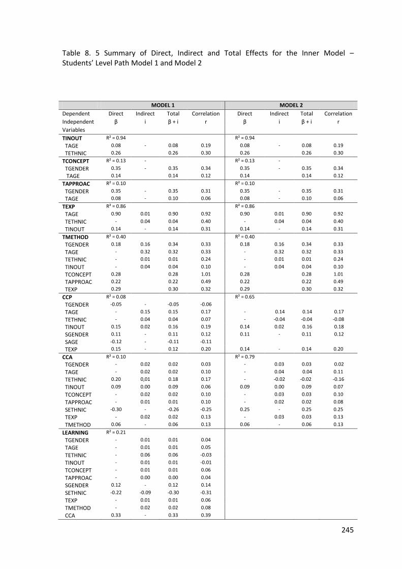
245

Table 8. 5 Summary of Direct, Indirect and Total Effects for the Inner Model – Students’ Level Path Model 1 and Model 2

MODEL 1 MODEL 2

Dependent Direct Indirect Total Correlation Direct Indirect Total Correlation

Independent β i β + i r β i β + i r

Variables

TINOUT R² = 0.94 R² = 0.94

TAGE 0.08 - 0.08 0.19 0.08 - 0.08 0.19

TETHNIC 0.26 0.26 0.30 0.26 0.26 0.30

TCONCEPT R² = 0.13 - R² = 0.13 -

TGENDER 0.35 - 0.35 0.34 0.35 - 0.35 0.34

TAGE 0.14 0.14 0.12 0.14 0.14 0.12

TAPPROAC R² = 0.10 R² = 0.10

TGENDER 0.35 - 0.35 0.31 0.35 - 0.35 0.31

TAGE 0.08 - 0.10 0.06 0.08 - 0.10 0.06

TEXP R² = 0.86 R² = 0.86

TAGE 0.90 0.01 0.90 0.92 0.90 0.01 0.90 0.92

TETHNIC - 0.04 0.04 0.40 - 0.04 0.04 0.40

TINOUT 0.14 - 0.14 0.31 0.14 - 0.14 0.31

TMETHOD R² = 0.40 R² = 0.40

TGENDER 0.18 0.16 0.34 0.33 0.18 0.16 0.34 0.33

TAGE - 0.32 0.32 0.33 - 0.32 0.32 0.33

TETHNIC - 0.01 0.01 0.24 - 0.01 0.01 0.24

TINOUT - 0.04 0.04 0.10 - 0.04 0.04 0.10

TCONCEPT 0.28 0.28 1.01 0.28 0.28 1.01

TAPPROAC 0.22 0.22 0.49 0.22 0.22 0.49

TEXP 0.29 0.30 0.32 0.29 0.30 0.32

CCP R² = 0.08 R² = 0.65

TGENDER -0.05 - -0.05 -0.06

TAGE - 0.15 0.15 0.17 - 0.14 0.14 0.17

TETHNIC - 0.04 0.04 0.07 - -0.04 -0.04 -0.08

TINOUT 0.15 0.02 0.16 0.19 0.14 0.02 0.16 0.18

SGENDER 0.11 - 0.11 0.12 0.11 - 0.11 0.12

SAGE -0.12 - -0.11 -0.11

TEXP 0.15 - 0.12 0.20 0.14 - 0.14 0.20

CCA R² = 0.10 R² = 0.79

TGENDER - 0.02 0.02 0.03 - 0.03 0.03 0.02

TAGE - 0.02 0.02 0.10 - 0.04 0.04 0.11

TETHNIC 0.20 0,01 0.18 0.17 - -0.02 -0.02 -0.16

TINOUT 0.09 0.00 0.09 0.06 0.09 0.00 0.09 0.07

TCONCEPT - 0.02 0.02 0.10 - 0.03 0.03 0.10

TAPPROAC - 0.01 0.01 0.10 - 0.02 0.02 0.08

SETHNIC -0.30 - -0.26 -0.25 0.25 - 0.25 0.25

TEXP - 0.02 0.02 0.13 - 0.03 0.03 0.13

TMETHOD 0.06 - 0.06 0.13 0.06 - 0.06 0.13

LEARNING R² = 0.21

TGENDER - 0.01 0.01 0.04

TAGE - 0.01 0.01 0.05

TETHNIC - 0.06 0.06 -0.03

TINOUT - 0.01 0.01 -0.01

TCONCEPT - 0.01 0.01 0.06

TAPPROAC - 0.00 0.00 0.04

SGENDER 0.12 - 0.12 0.14

SETHNIC -0.22 -0.09 -0.30 -0.31

TEXP - 0.01 0.01 0.06

TMETHOD - 0.02 0.02 0.08

CCA 0.33 - 0.33 0.39

246

Table 8.5 Continued

SURFACE

R² = 0.11

TGENDER - 0.01 0.01 0.01

TAGE - 0.01 0.01 0.06

TETHNIC - -0.01 -0.01 0.04

TINOUT - 0.03 0.03 -0.06

TCONCEPT - 0.01 0.01 0.07

TAPPROAC - 0.01 0.01 0.06

SGENDER 0.16 - 0.16 0.17

SETHNIC - 0.07 0.07 0.26

TEXP - 0.01 0.01 0.06

TMETHOD - 0.03 0.03 0.11

CCA 0.28 - 0.28 0.28

ACHIEVING R² = 0.64

TGENDER - 0.01 0.01 0.32

TAGE - 0.01 0.01 0.05

TETHNIC - -0.01 -0.01 0.02

TINOUT - 0.04 0.04 -0.01

TCONCEPT - 0.01 0.01 0.06

TAPPROAC - 0.01 0.01 0.04

SGENDER - 0.11 0.11 0.15

SETHNIC - 0.10 0.10 0.30

TEXP - 0.01 0.01 0.06

TMETHOD - 0.04 0.04 0.08

CCA 0.20 0.20 0.40 0.40

SURFACE 0.72 - 0.72 0.78

DEEP R² = 0.90

TGENDER - 0.01 0.01 0.04

TAGE - 0.01 0.01 0.04

TETHNIC - -0.01 -0.01 0.01

TINOUT - 0.04 0.04 0.01

TCONCEPT - 0.01 0.01 0.04

TAPPROAC - 0.01 0.01 0.03

SGENDER - 0.11 0.11 0.12

SETHNIC 0.01 0.10 0.11 0.30

TEXP - 0.01 0.01 0.05

TMETHOD - 0.04 0.04 0.05

CCA 0.23 0.37 0.40 0.40

SURFACE - 0.67 0.67 0.57

ACHIEVE 0.93 - 0.93 0.95

SOUTCOME R² = 0.46 R² = 0.48

TGENDER - 0.01 0.01 0.05 - 0.01 0.01 0.05

TAGE - 0.01 0.01 0.10 - 0.01 0.01 0.10

TETHNIC - 0.06 0.06 0.00 - -0.01 -0.01 0.00

TINOUT 0.05 0.05 0.02 0.05 0.05 0.02

TCONCEPT - 0.00 0.00 0.05 - 0.00 0.00 0.05

TAPPROAC - 0.00 0.00 0.05 - 0.00 0.00 0.05

SGENDER - 0.07 0.07 0.11 - 0.08 0.08 0.11

SETHNIC -0.20 -0.20 -0.02 - -0.20 -0.35 -0.34

TEXP - 0.00 0.00 0.11 - 0.00 0.00 0.11

TMETHOD - 0.02 0.02 0.05 - 0.03 0.03 0.05

CCA 0.10 0.36 0.35 0.11 0.11 0.02

LEARNING 0.59 - 0.59 0.66

SURFACE - 0.34 0.51 0.50 0.20 0.20 0.02

ACHIEV - 0.48 0.47 0.66 - 0.48 0.47 0.66

DEEP 0.51 - 0.51 0.66 0.53 - 0.53 0.03

247

8.4 Inner Model–Students’ Level Model 1 and 2

The inner or structural model results specify the strength of relationships between one

LV regressed on other LVs (Rintaningrum et al., 2009). In PLSPATH program, the

command lines to indicate these relationships are termed ‘MODEL’. Any path between

the LVs will be removed from the model if the path does not showed meaningful and

adequate influence (Darmawan, 2003; Rintaningrum et al., 2009). The indicators

commonly used to delete or remove paths which are not significant in the inner model,

are: a) regression coefficient (beta), b) correlation coefficient (r), c) tolerance, d)

jackknife means (JknMean), and e) jackknife standard error(JknStd). To check the

predictive strength of the inner model R-square (R²) was used.

One of the widely used indicators is Beta, which is the coefficient of the direct effect

between one latent variable and another latent variable. Sellin (1989) suggested that

beta coefficients are generally acceptable with a value of 0.05 or larger for a large a data

set, or 0.10 for a small data set. According to Sellin and Keeves (1997), the larger the β,

value, the larger is the effect on the path model. Any direct path that is less than 0.10,

needs to be removed from the path model. This process needs to be undertaken

iteratively until all non significant paths are removed.

The jackknife mean is the mean of the path coefficients obtained in each jackknife cycle.

The jackknife standard error is the estimated error associated with each path coefficient.

Correlation coefficients involve the zero-order or the product moment correlation

coefficient between the given independent (predictor) latent variables and the

dependents (criterion) latent variables (Sellin, 1989). Although in PLSPATH analysis the

results do not provide a statistically significant test, Darmawan (2003, p. 82), has argued

248

that ‘where an estimated coefficient is more than twice the value of its jackknife

standard error, the coefficient can be considered to be statistically significant at

approximately the five per cent level of probability’.

The following discussions are based on the indices that presented in Table 8.5. Most of

the variables had β values greater than 0.05. These results revealed that the beta

coefficients for the inner model were acceptable.

Tolerance indicates the existence of multicollinearity and is calculated as the squared

multiple correlations between an independent LV and the set of remaining independent

LVs involved in the given inner model equations (Sellin, 1990). When the values are

larger than 0.50, the relationship between the LVs and the associated LVs needs to be

reconsidered. In these inner model results, the tolerance is an index that measures the

relative amount of multicollinearity. The inner results in Table 8.5 showed that, most of

the values of tolerance are less than 0.50. The next section describes the effects on the

Latent Variable that involves in the path model of the endogenous and exogenous

variables in the model.

The Effect ON the variable in the Inner Model–Student Level Path.Models 1and 2

This section discussed the relationships of the latent and manifest variables shown in

the Students’ Level Path Models in Figures 8.1 and 8.2. The discussions focuses on direct

and indirect effects demonstrated.

TInout (In-field/ out-of-field teacher)

R² = 0.94

Teachers’ Age (TAge) effect on TInout (β = 0.08, SE= 0.03)

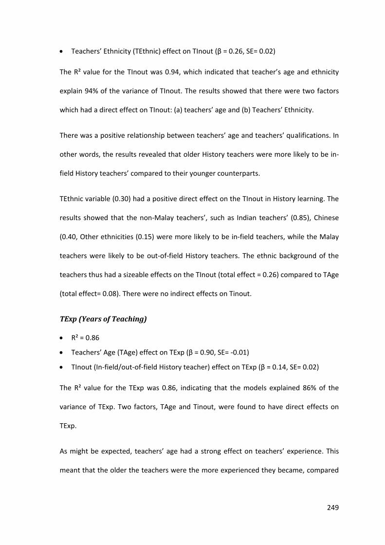
249

Teachers’ Ethnicity (TEthnic) effect on TInout (β = 0.26, SE= 0.02)

The R² value for the TInout was 0.94, which indicated that teacher’s age and ethnicity

explain 94% of the variance of TInout. The results showed that there were two factors

which had a direct effect on TInout: (a) teachers’ age and (b) Teachers’ Ethnicity.

There was a positive relationship between teachers’ age and teachers’ qualifications. In

other words, the results revealed that older History teachers were more likely to be in-

field History teachers’ compared to their younger counterparts.

TEthnic variable (0.30) had a positive direct effect on the TInout in History learning. The

results showed that the non-Malay teachers’, such as Indian teachers’ (0.85), Chinese

(0.40, Other ethnicities (0.15) were more likely to be in-field teachers, while the Malay

teachers were likely to be out-of-field History teachers. The ethnic background of the

teachers thus had a sizeable effects on the TInout (total effect = 0.26) compared to TAge

(total effect= 0.08). There were no indirect effects on Tinout.

TExp (Years of Teaching)

R² = 0.86

Teachers’ Age (TAge) effect on TExp (β = 0.90, SE= -0.01)

TInout (In-field/out-of-field History teacher) effect on TExp (β = 0.14, SE= 0.02)

The R² value for the TExp was 0.86, indicating that the models explained 86% of the

variance of TExp. Two factors, TAge and Tinout, were found to have direct effects on

TExp.

As might be expected, teachers’ age had a strong effect on teachers’ experience. This

meant that the older the teachers were the more experienced they became, compared

250

to the younger History teachers. Similarly, the results showed that in-field History

teachers were more experience compared to out-of-field History teachers.

In addition, teachers’ age and teachers’ ethnicity also influenced teaching experience

indirectly through the in-field/out-of-field constructs.

TCont (Teaching Conceptions)

R² = 0.13

Teacher Gender (TGender) effect on TCont (β = 0.35, SE= 0.00)

Teacher Age (TAge) effect on TCont (β = 0.14, SE= 0.01)

The R² value for the TCont was 0.13, which indicated that the models explained 13% of

the variance of TCont. There were two factors that directly influenced the teacher

conceptions (TCont). They were TGender and TAge and both were positive effects.

The results indicated that female History teachers tended to have stronger teaching

conceptions towards History teaching in the classroom compared to male teachers. The

effect of age on teaching conception indicated that older History teachers were more

likely to have stronger teaching conceptions towards History teaching in the classroom

compared to the younger teachers.

TApp (Teaching Approaches)

R² = 0.10

Teacher Gender (TGender) effect on TCont (β = 0.35, SE= 0.00)

Teacher Age (TAge) effect on TCont (β = 0.14, SE= 0.01)

The R² value for the TApp was 0.10, indicating that the models explained 10% of the

variance of TApp. There were two factors that directly influenced the teaching

approaches (TApp), TGender and TAge. Both of these variables positively influenced the

251

TApp. The result indicated that female History teachers were more likely to employ an

effective teaching approach compared to their male counterparts. In addition, these

results also indicated that older History teachers were more likely to adopt higher level

teaching methods in the classroom.

TMet (Teaching Methods)

R² = 0.40

Teachers’ Gender (TGender) effect on TMet (β = 0.18, SE= 0.03)

Teaching Conception (TCont) effect on TMet (β = 0.28, SE= -0.00)

Teachers’ Approaches (TApp) effect on TMet (β = 0.22, SE= 0.02)

Teachers’ Years’ of Teaching (TExp) effect on TMet (β = 0.29, SE= 0.04)

The R² value for the TMet was 0.40, indicating that the model explained 40% of the

variance of TMet. In this path model, there were two manifest variables reflected the

teacher teaching method; effective (0.97) and active (0.93) teaching methods. There

were four factors that directly influenced teachers’ teaching methods (TMet): the

TGender, TCont, TApp, and TExp.

All these variables had positive influence on the teaching approaches. The results

showed that female History teachers employed more effective and active teaching

methods compared to male History teachers.

The positive relationship between TMet and teaching conceptions indicated that those

History teachers who had higher teaching conceptions employed more effective and

active teaching methods.

252

The third variable that directly influenced the TMet were TApp. The teaching

approaches in these two models were refelected by two manifest variables: included in

the model. Which were a) the Information transfer/teacher-focused (TInfoTra) (0.93)

and b) conceptual change/student-focused (TConChan) (0.95). The results indicated that

the teachers who adopted a higher level teaching approach were more likely to

implement more effective and active teaching methods. Beside this, as the number of

years teaching increased, teachers were likely to employ more effective and active

teaching methods.

Table 8.5 showed the indirect effects of latent variables that influenced History teacher

Teaching Method (TMet). The result indicates that indirect effect of TGender (i=0.16)

through TAge (i=0.32); TEthnic (i = -0.01) through TMet (0.40).

Teacher Gender (TGender) (i = 0.16)


Teacher Ethnic (TEthnic) (i = -0.01))

Teacher In-field/ out-of-field (TInout) (i = 0.04)

TEthnic showed the smallest effects (i = -0.01) compared to other variables. TGender

showed indirect effects on TMet (0.16) in addition to the direct effect discussed above.

The effect of gender on teaching methods through TApp was 0.16. This meant that

female teachers who were high on teaching approaches were more likely to employed

have effective and active teaching method in History lesson. In addition, TAge

influenced teaching method through TApp (i=0.32). TInout also had an indirect effect on

TMet (i = 0.04) through TExp.

253

However, the TEthnic variable (-0.01) had very small negative indirect effects on the

teaching methods (TMet) in History learning. This result indicated that Indian teachers

(0.85), were less likely to employ effective and active teaching methods, than those of

Malay, Chinese and other ethnic backgrounds.

CCP (Classroom Climate Preferred)

R² = 0.08

Teacher Gender (TGender) effect on CCP (β = -0.05, SE= 0.02)

TInout (In-field/out-of-field History teacher) effect on CCP (β = 0.14, SE= 0.02)

Students’ Gender (SGender) effect on CCP (β = 0.11, SE= 0.03)

Students’ Age (SAge) effect on CCP (β = -0.12, SE= 0.02)

Teachers’ Year of Teaching (TExp) effect on CCP (β = 0.15, SE= 0.05)

The R² value for the CCP was 0.08, indicating that the model explained 8% of the

variance of CCP. There were five factors that directly influenced the classroom climate

preferred (CCP): TGender, TInout, SGender, SAge and TExp. Besides having direct effects,

CCA had also indirectly effects from TAge (i = 0.15), TEthnic (i = 0.04), and TInout

(i = 0.14).

The direct relationship between CCP and TGender (teachers’ gender) indicated that

students taught by the female History teachers were more likely to prefer classrooms

that higher degree of personalisation (0.98), participation (0.93), and investigation (0.69)

but less emphasis on the independence (-0.20), and differentiation (-0.88).

Students taught by in-field History teachers’ were more likely to have classes in which,

on average, students preferred to experience more personalisation, participation and

investigation, but less the independence and differentiation in their History classroom.

254

The results showed a positive relationship between SGender and CCP. This result

indicated that classrooms that had higher proposition of girls were more likely to prefer

more personalisation, participation and investigation in their learning activities but less

independence, and differentiation compared to History classes that had more boys. In

addition, those students in classes taught by experienced History teachers were more

likely to want more personalisation, participation and investigation but less

independence, and differentiation as their preferred classroom environment (CCP),

compared to students under novice History teacher. The results also indicate that the

older the students were the more likely they wanted to experience personalisation,

participation and investigation and but less independence and differentiation in their

History classroom.

As shown in the path diagram in Figure 8.1 the preferred classroom climate (CCP) were

indirectly influenced by three variables. These were:


Teacher Ethnic (TEthnic) (i = 0.04)

TInout (In-field/out-of-field History teacher) (i = 0.02)

The preferred classroom environment (CCP), variable was influenced indirectly by

teacher age (TAge) (0.15) and TInout (0.02) through the teacher experience (TExp)

construct. The results indicated that older teacher who more likely in-field History

teachers tended to have classes where students preferred more personalisation (0.98),

participation (0.93), and investigation (0.69) but less independence (-0.20), and

differentiation(-0.88), compared to students under out-of-field History teachers. CCP

255

was also influence indirectly by Teachers’ Ethnicity through the in-field/out-of-field

construct (0.04).

TEthnic also had positive indirect effects on ACHIEV. Although, it is a relatively small

effect (0.04.) It can be interpreted that students under Indian teachers (0.85), were

more likely to prefer personalisation, participation and investigation but less

independence and differentiation in their History classroom, than students under

teachers of Malay (D) , Chinese (0.38) and other ethnic (0.16) background.

CCA (Classroom Climate Actual)

R² = 0.10

Teacher Ethnic (TEthnic) (β = 0.17, SE = 0.02) on CCA

TInout (In-field/out-of-field History teacher) effect on CCA ( = β 0.09, SE= 0.02)

Student Ethnicity (SEthnic) effect on CCA (β = -0.26, SE= 0.03)

Teaching Methods (TMet) effect on CCA (β = 0.06, SE= 0.02)

The R² value for the CCA was 0.10, which indicated that the model explained 10% of the

variance of CCA. There were four factors that were found to have direct effects on

CCA;a) TEthnic b) TInout, c) SEthnic, and d) TMet.

TEthnicity (0.20) had a direct effect on the actual classroom climate (CCA) in History

learning. The results indicated that students under Indian teachers (0.85), were more to

experience participation (0.86), investigation (0.75) and personalisation (0.64) and less

independence (-0.50), and differentiation (-0.57) in their actual learning History

classroom climate.

256

There was a positive relationship between TInout and CCA. This result indicated that

that ‘in-field’ History teachers were more likely to have classes in which students

actually experienced more participation (0.86), investigation (0.75) and personalisation

(0.64), but less independence (-0.50), and differentiation (-0.57) compared to students

in classes under out-of-field History teachers.

The results showed a negative relationship between SEthnic and CCA. The negative sign

indicates that Chinese (0.99), and those of other ethnic (0.04) background, experienced

more participation (0.86), investigation (0.75) personalisation (0.64), and less

independence (-0.50), and differentiation (-0.57) in their actual History classroom

environment compared to Malay and Indian students. In addition, the results showed a

small positive relationship between CCA and teachers who employed effective and

active teaching methods.

Indirect Effect on CCA were observed from the following variables:


Teacher Age (TAge) (i = 0.15))



TGender had an indirectly effect on the CCA through Teaching Methods (0.15). This

result indicated that in the actual classroom environment female History teachers were

more likely to encourage participation (0.86), investigation (0.75) personalisation (0.64),

and but less independence (-0.50), and differentiation (-0.57) compared to male

teachers.

257

TAge had an indirect effect on the classroom climate actual (CCA) through teacher

Approaches (TAPP) and Teaching Method (TMet). The results revealed that older

teachers who were more likely to be in-field History teachers tended to have classes

where students, on average, experienced higher levels of participation (0.86),

investigation (0.75) personalisation (0.64), but lower levels of independen (-0.50), and

differentiation (-0.57) in their actual classroom. In addition to this indirect effect, CCA

was also influenced by Teacher Ethnicity (Ethnicity) through in-field/out-of-field

construct (0.04) and TInout through Teacher Experience (0.02).

The Effect ON the variable in the Inner Model- Students’ Level Path Model 1

This section discusses variables in the inner models which had an effect on Student

Approaches to Learning as it was set up in Model 1, where all learning approaches were

combined into a single variables ‘SLearning’.

Student Approaches to Learning (SLearning)

R² = 0.21

Student Gender (SGender) effect on (SLearning) (β = 0.12, SE= 0.02)

Student Ethnicity (SEthnic) effect on (SLearning) (β = -0.23, SE= 0.02)

Classroom Climate Actual (CCA) effects on (SLearning) (β = 0.33, SE= 0.03)

The R² value for the SLearning was 0.21, indicating that the Student Level Path Model

explained 21% of the variance of SLearning in this model. There were six manifest

variables reflecting students’ approaches to learning. They were (1) deep, (2) surface,

and (3) achieving. There were three factors that were found to have direct effects on

SLearning namely; (a) SGender (b) SEthnic, and (c) CCA. (see Figure 8.1).

Results showed that girls were more likely adopted higher order learning approaches.

258

SEthnic had a direct effect on SLearning. Path analysis results showed a positive

influence of CCA on SLearning, This result indicated that the actual classroom

environments of students positively affected their approaches to learning.

The analysis for Students’ Level path Model 1 revealed nine variables that have indirect

effects on Students’ Learning. There are listed below:





Teaching Conception (TCont) (i = 0.01) effect on SLearning (R²= 0.21)

Teacher Approaches (TApp) (i = 0.00)

Student Ethnicity (SEthnic) (i = -0.09)

Teacher Year of Teaching (TExp) (i = 0.01)

Teaching Methods (TMet) (i = 0.02)

Only one of these is discussed. Teacher Age was found to have and indirect effect on

student approaches to learning (SLearning). The results show positive relationships

between SLearning and TAge through CCA construct (0.06). This result indicated that

students’ under older teachers who were more likely to be in-field History teachers

tended to adopt high order learning approach.

Students’ Perception of History Learning Outcome (SOutcome)

R² = 0.46

TInout (In-field/out-of-field History teacher) effect on SOutcome (β = 0.05, SE= 0.02)

Student Ethnicity (SEthnic) effect on SOutcome (β = 0.20, SE= 0.02)

Classroom Climate Actual (CCA) effect on SOutcome (SLearning) (β = 0.10, SE= 0.02)

Student Learning Approaches (SLearning) effect on SOutcome (β = 0.59, SE= 0.03)

259

The R² value for the SOutcome variables was 0.46, indicating that the Student Level Path

Model 1 explained 46% of the variance of SOUTCOME. Four factors were found to have

direct effects on SOutcome: (a) Tinout (b) SEthnic, and (c) CCA, and (d) SLearning.

SLearning (β=0.59, SE= 0.03) had the strongest direct effect on History learning outcome

(SOutcome), demonstrating that the learning approach which student adopted had a

considerable effect on their perceptions of History learning outcome (SOutcome). The

results for Classroom Climate Actual (0.10) was smaller, and for out-of-field teachers

(0.05) even less, but suggested that students in more positive classroom climates, and

under in-field teachers, were to some extent more likely to have higher perceptions of

History learning objectives.

Eleven variables had indirect effects on students learning outcomes. These were:





Teaching Conception (TCont) (i = 0.001)


Student Gender (SGender) (i = 0.07)

Student Ethnicity (SEthnic) (i = -0.35)


Teaching Methods (TMet) (i = 0.02)

Classroom Climate Actual (CCA) (i = 0.28)

Most of these effects were quite small and are not discussed further.

260

The Effect ON the variable in the Inner Model- Student Level Model 2

This section discusses variables in the inner models which had an effect on Students’

Learning Approaches as it was set up in Model 2, where all learning approaches discuss

here.

SURFACE (Surface Learning Approaches)

R² = 0.11

Student Gender (SGender) effect on SURFACE (β = 0.16), SE= 0.02)

Classroom Climate Actual (CCA) effect on SURFACE (β = 0.28, SE= 0.03)

The R² value for the SURFACE was 0.11, which indicated that the Student Level Path

Model 2 explained 11% of the variance of SURFACE. Figure 8.2 showed that SURFACE

learning approach was influenced by students’ gender (0.20) and CCA (0.30). These

variables were found to have positive direct effects on SURFACE learning approach.

Results showed that girls were more likely to adopt surface learning approaches

compared to boys. The results also indicated a positive relationship between CCA and

SURFACE, suggesting that the Accual Classroom Climate experienced by the students,

directly influenced their adoption of SURFACE learning approach.

The analysis for Students’ Level Path Model 2 revealed nine other variables were found

to have indirect effects on Surface Learning Approaches namely;



Teacher Ethnicity (TEthnic) (i = -0.01)




261

Students’ Ethnicity (SEthnic) (i = 0.10)

Teachers’ Years of Teaching (TExp) (i = 0.01)

Teacher Method (TMet) (i = 0.03))

Most of the variables were showing small indirect effects on SURFACE learning

approach.

ACHIEV (Achieving Learning Approaches)

Table 8.5 showed that;

R² = 0.64

Classroom Climate Actual (CCA) effect on ACHIEV (β = 0.20, SE= 0.01)

Surface Approaches to Learning (SURFACE) effect on ACHIEV (β = 0.72, SE= -0.00)

The R² value for the ACHIEV was 0.64, which indicated that the Student Level Path

Model 2 explained 64% of the variance of ACHIEV. The Actual Classroom Climate (CCA)

and SURFACE learning approach were found to have positive and significant direct

effect on ACHIEV. CCA had a direct effect (β = 0.20), suggesting that the Actual

Classroom Climate experienced by the students directly effected their adoption of the

Achieving Learning Approaches and indirectly (i = 0.20) to adopt the achieving learning

approach through SURFACE.

Another factor with a direct influence on History learning approaches was SURFACE.

This result suggested that those students who adopted SURFACE approaches to learning

were likely to also employ ACHIEV approaches to learning during the History lesson.

There were eleven other variables which had indirect effect on Achieving Learning

Approaches. There are listed below:


262


Teacher Ethnic (TEthnic) (i = -0.01)





Students Ethnic (SEthnic) (i = 0.10)


Teacher Method (TMet) (i = 0.04)


Most of these variables showed a very small indirect effect and not discussed further.

DEEP (Deep Learning Approaches)

R² = 0.90

Students Ethnic (SEthnic) effect on DEEP(β = 0.01, SE= 0.00)

Classroom Climate Actual (CCA) effect on DEEP (β = 0.23, SE= 0.02)

Achieving Approaches to Learning (ACHIEV) effect on DEEP (β = 0.93, SE= -0.00)

The R² value for the DEEP was 0.90, which indicated that the Student Level Path Model

2 explained 90% of the variance of DEEP. There were three variables found to have

direct effect on deep approach to learning (DEEP). Students’ Ethnicity and Classroom

Climate Actual both positive both effects on DEEP approach. SEthnic have a direct effect

of 0.01 and an indirect effect 0.10. The CCA has a direct effect of 0.03, and an indirect

effect of 0.40. The indirect effects were larger than the direct effects for both variables.

On the other hand, ACHIEV (0.93) showed a stronger effect directly on DEEP approach

to learning. The direct effects of ACHIEV revealed that students’ with ACHIEVE approach

263

to learning were likely to employ the DEEP approach to learning in the History

classroom.

Thirteen variables were shown to have indirect effect on the Deep Learning Approaches.

There were listed below:



Teacher Ethnic (TEthnic) (i = -0.01)









Surface Approaches to Learning (SURFACE) (i = 0.67)

Achieving Approaches to Learning (ACHIVE) (i = 0.93)

CCA showed indirect effects on DEEP. This result suggested that the Actual Classroom

Climate experienced by the students had considerable indirect effect on their adoption

of Deep Learning Approach through ACHIEV (i= 0.40). In addition to this, SURFACE

(i=0.67) had a stronger indirect effects on DEEP approach in learning through ACHIEVE.

This result indicates that students’ who employed Surface learning approach were likely

to adopt the DEEP and ACHIEVING learning approach in the History classroom. The

largest indirect effect was Achieving Approaches to Learning. Indicating that student

who had reached this level of learning were most likely to adopt Deep Approaches to

Learning in the History classroom.

264

Students Perception of History Learning Objective (SOutcome)

R² = 0.48

Classroom Climate Actual (CCA) effect on SOutcome (β = 0.11, SE= 0.02)

Surface Approaches to Learning (SURFACE) effect on SOutcome (β = 0.16, SE= 0.02)

Deep Approaches to Learning (DEEP) effect on SOutcome (β = 0.51, SE= 0.03)

TInout (In-field/out-of-field History teacher) effect on SOutcome (β = 0.05, SE= 0.02)

The R² value for the SOutcome was 0.48, which indicated that the model explained 50%

of the variance of SOutcome. There were four variables found to have direct effect on

students’ perception of History learning (SOutcome) namely, CCA, SURFACE, and DEEP,

and TIout (In-field/out-of-field).

Overall, the sizeable direct effect on SOutcome was from DEEP (0.51). This result (see

Figure 8.2) indicated that students that employed DEEP learning approach were likely to

perceive learning History at a higher or level of appreciation to the efforts and the

contributions of individuals who struggled for independence and development of the

country (0.97), individual (0. 96) and community (0.98).

The CCA result indicated that the actual classroom climate experienced by students

influenced their perceptions on how well the History learning achieved its objectives.

SURFACE (0.20) also have positive effects on SOutcomes. The results indicated that

classroom in which more students adopted a SURFACE approach were more likely to

have positive perception of History learning outcomes (SOutcomes). This result could be

accounted for by rote learning which is a mark of Surface approach to learning. In

addition, TIout (in-field and out-of-field) had a small direct and indirect effects on

History learning outcomes (SOutcomes).

265

There were thirteen variables which had indirect effect on SOutcome. Most of these

had small effects and are not discussed further.

Teacher Gender (TGender) (i = 0.01))


Teacher Ethnic (TEthnic) (i = -0.06))




Student Gender (SGender)





Surface Approaches to Learning (SURFACE) (i =0.34)

Achieving Approaches to Learning (ACHIEV) (i =0.48)

However, two variables namely Surface and Achieving Learning Approach were found

to have indirect influences on SOutcomes through DEEP. The result could be interpreted

that students who employed achieving learning approaches tended to have more

positive perceptions of History learning outcomes (SOutcomes). In addition to its direct

effect SURFACE was found to have indirect effect on SOutcome (0.34).

8.5 Summary of Analysis for Students’ Level – Path Models 1and 2

This section summarized the main findings from path analysis for Models 1 and 2. In

Model 1, SLEARNING was taken as a single variable (see Figure 8.1). In Model 2,

however, the ‘Learning Approaches’ variables were discussed as six separate variables:

266

surface motive, deep motive, achieving motive, surface strategy, deep strategy,

achieving strategy (See Figure 8.2). The other LVs and MVs were the same in both

models.

(a) For Conceptions of teaching, the results indicated that there were two direct effects:

by Teacher Gender and Teacher Age. The results showed that Teacher Gender had

larger direct effects compared to Teacher Age. This meant that female History teachers

tended to have higher conceptions toward History teaching compared to the male

History teacher.

(b) In relation to Teaching approaches, the results revealed positive direct influence of

Teacher Gender and Teacher Age on Teaching Approaches. Thus, female teachers were

more likely to employ effective and active teaching methods compared to their male

counterparts.

(c) In case of TInout (In-field/ out-of-field teacher), there were two factors that were

found to have a direct influence on TInout namely: (a) teachers’ age and teachers’

ethnicity. The results showed that Teacher Ethnicity had a positive direct effect on

TInout (In-field/ out-of-field teacher), in History learning. Which meant that non-Malay

teachers, such as those of Indian, Chinese, and other background were more likely to be

in-field History teachers group, and Malays to be out-of-field History teachers. The

ethnic background of the teachers had a sizeable effects on the TInout (In-field/ out-of-

field teacher), compared to Teacher Age

(d) For Teaching Approaches, the teacher variables (TGender, TCont, TApp, and TExp)

were shown to have positive influence. The results showed that female History teacher

267

employed more effective and active of teaching methods compared to male History

teachers. History teachers who had higher teaching conception tended to employ more

effective and active teaching methods. In addition, the results revealed that as teachers

became more experiences over the years they were likely to employ effective and active

teaching methods.

(e) In relation to, Teaching experience (years of teaching), the results indicated a

positive relationship with two variables: teachers’ age and teacher TInout (‘in-field’ and

‘out-of-field’). In the case of teachers’ age, the direct effect was considerably, indicating

that as teachers’ age increased they were more likely to become experienced compared

to the younger History teachers. In addition, in-field History teachers were shown to be

more experienced in teaching History compared to out-of-field History teachers.

(f) For Preferred Classroom Climate (CCP), the direct effect on CCP and TGender

(teacher gender) indicated that students taught by female History teachers were more

likely to prefer a classroom that had a high degree of personalisation participation, and

investigation but less on the independence, and differentiation Students taught by older

History teacher who were more experienced and more likely to be in-field, were more

likely to be in classes in which, on average, students preferred more personalised,

participation and investigation activities but less independent and differentiation

activities in their History classroom. The results also indicated that classrooms that had

high proportion of girls were more likely to prefer personalised, participation and

investigative learning activities but less independent, and differentiation activities in

their classroom environment, compared to those that classes had more boys.

268

(g) In relation to, Actual Classroom Climate the results indicated that students under

Indian teachers, were more likely to experienced participation investigation and

personalised learning activities, and less on the independence, and differentiation

during in-field History There was also evidence that in-field History teachers were more

likely to have classes in which students actually experienced more participation,

investigation, and personalisation, but less independence, and differentiation,

compared to out-of-field History teachers. The results also showed a negative

relationship between Student Ethnic and Actual Classroom Climate. The negative sign

indicated that non-Malay students such as Chinese, Indian and those of other ethnic

backgrounds, experienced more participation, investigation, personalisation, and less

independence, and differentiation learning activities in their actual History classroom.

(h) In relation to the variable Student Approaches to Learning, results showed that girls

were more likely to adopt high order learning approaches. Furthermore, Student Ethnic

had a direct effect on Student Learning. In other words, Indian students were more

likely to adopt high order learning approaches than those of other backgrounds. These

results provided evidence that the actual classroom environment of students was

positively linked with the approaches to learning they adopted.

(i) Surface Learning Approach was influenced directly by Student Gender and Actual

Classroom Climate. This result showed that actual classroom environment had a strong

influence on students’ adoption of surface learning. In addition, girls were more likely

than boys to adopt surface learning approaches.

(j) In relation to, Achieving Learning Approaches (ACHIEV), the results showed that

Surface learning approach had strong indirect effects on Achieving approach to learning.

269

This result suggested that students who experienced more Surface approaches to

learning were more likely to adopt the achieving approaches in learning History.

Another indirect factor was Surface. This result suggested that those students who

adopted Surface approaches to learning were likely to employ Achieving approaches to

learning during the History lesson.

(k) For Deep Learning Approach (DEEP), the results showed that the Achieving Approach

to learning had the biggest direct effects, compared to students’ ethnicity and actual

classroom climate. This result indicated that students’ with Achieving approach to

learning were more likely to employ the DEEP approach to learning in the History

classroom.

(l) In the case of the, Students’ Perception of History learning (SOutcome), there were

three LVs with the direct effects DEEP showed the largest direct effect compared to the

other direct effects, Actual Classroom Climate and Surface learning approach. This result

indicated that students who employed the DEEP learning approach were more likely to

perceive that History learning outcomes had been achieved. In addition, students in

classrooms where, on average, students adopted the Surface approach to learning were

more likely to have positive perceptions of History learning outcomes.

In the case of the PLSPATH analysis of the students level data, both models investigated

showed one comparatively small direct effect between Teachers’ qualifications (out-of-

field/in-field) and Students’ History Learning Outcomes. The implication of the results is

considered further in the concluding discussion of Chapter 10. The following chapter

reports the results of the Hierarchical Linear Modeling (HLM) analysis which was carried

270

out as the next stage of the investigation, to take account of the two levels of variables -

teachers and students.

271

Chapter 9 Hierarchical Linear Modeling

Analysis ________________________________________________________________________

9.1 Introduction

This chapter presents Hierarchical Linear Modeling (HLM) analysis: the procedure of

HLM, model building, model trimming and the results of the HLM analysis. In the two

previous chapters, single level path analyses were carried out using PLSPATH modeling.

However, this study involves multilevel data where a number of students at the lower

layer belonged to one classroom and a teacher in the upper layer. With data from two

levels, HLM is an appropriate procedure to use for further analysis (Bryk & Raudenbush,

1992). As Braun, Jenkins, and Grigg (2006, p.6) affirmed, HLM is ‘a class of techniques

for analysing data having a hierarchical or nested structure’. Hence, HLM was employed

in this study to examine the impacts of both student and teacher characteristics on

students’ approaches to learning and perceived History learning outcomes at students’

level.

As mentioned in previous chapters the traditional approaches in to analysing two levels

of data have a number of shortcomings such as violation of the independence of data

assumptions, misestimated standard errors, as well as aggregation and disaggregation

bias. Nalaya (2010, p.194), added that ‘treating hierarchical data as single level data can

lead to flawed findings and biased estimations of effects’. The use of HLM can overcome

these limitations. In addition, HLM procedures make it possible to analyse variables at

both levels (teachers and students) concurrently. In this study, Two-Level Hierarchical

272

procedures were used to test the models. Level 1 is the student level and level 2 is the

teacher level. HLM 6 program was used in this analysis (Bryk & Raudenbush, 1992).

9.2 Variables used in the model

HLM program Version 6 (Raudenbush, et al., 2004) does not provide the formation of

latent variables (Darmawan, 2003). Therefore, SPSS 17 was used to calculate

component scores for each construct involved in the models. As a result, according to

Pedhazur (1997), most of the variables were in standardised forms, except for the

variables of GENDER, AGE and TIN-FIELD. Additionally, Perdhazur (1997) added that

standardised variables in the models allowed the direct comparison of coefficients of

variables within the HLM models. In this study GENDER was a categorical variable, which

was coded as Female = 1 and Male = 0. Variables SAGE and TAGE were used to record

the teachers’ and students’ age in years. TINFIELD was the teachers’ qualifications -‘in-

field’ or ‘out-of-field’ History teachers.

This study aimed to examine relationships between teachers’ and students’

characteristics and perceptions on various constructs. Variables used in the HLM

analysis were grouped into (a) students level variables, and (b) teachers’ level variables.

The list of variables used is presented in Table 9.1.

Variables at Level 1 (Students level) included :(a) students’ characteristics (age, gender,

ethnicity), (b) classroom climate Preferred, classroom climate Actual, (c) approaches to

learning (Surface, Achieving and Deep approaches), and (d) students’ perceptions of

History learning (SOutcomes) in teaching and learning History in the classroom. At Level

2 (Teachers level), the variables tested were: (a) the teachers’ individual characteristics

(age, gender, ethnicity), (b) teacher qualifications (in-field and out-of-field); (c) teacher

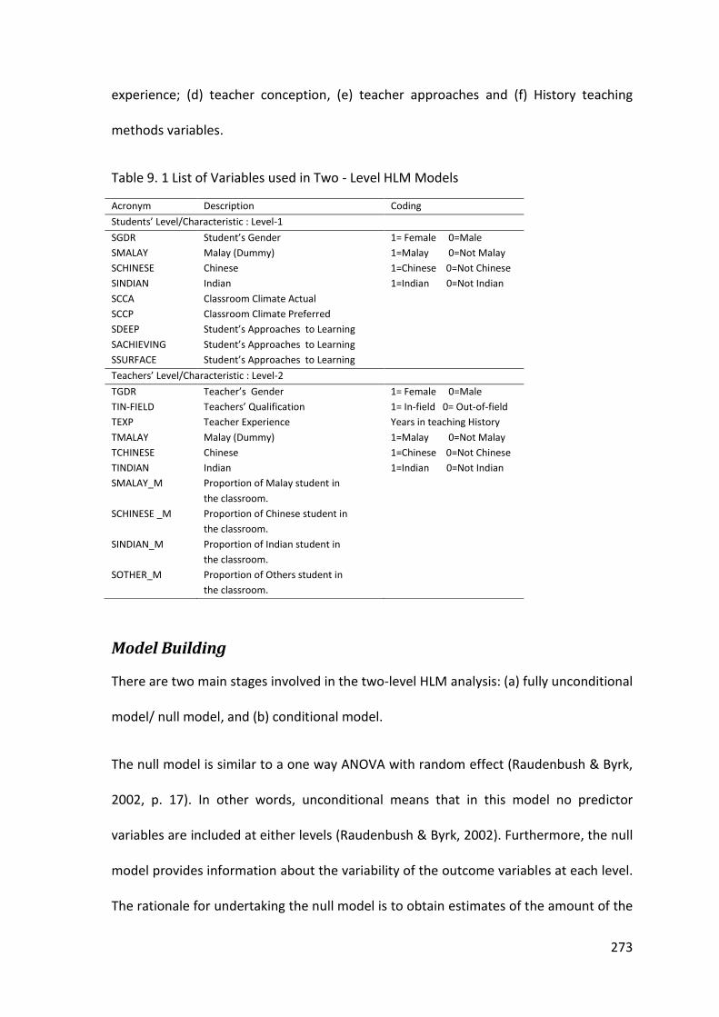
273

experience; (d) teacher conception, (e) teacher approaches and (f) History teaching

methods variables.

Table 9. 1 List of Variables used in Two - Level HLM Models

Model Building

There are two main stages involved in the two-level HLM analysis: (a) fully unconditional

model/ null model, and (b) conditional model.

The null model is similar to a one way ANOVA with random effect (Raudenbush & Byrk,

2002, p. 17). In other words, unconditional means that in this model no predictor

variables are included at either levels (Raudenbush & Byrk, 2002). Furthermore, the null

model provides information about the variability of the outcome variables at each level.

The rationale for undertaking the null model is to obtain estimates of the amount of the

Acronym Description Coding

Students’ Level/Characteristic : Level-1

SGDR Student’s Gender 1= Female 0=Male

SMALAY Malay (Dummy) 1=Malay 0=Not Malay

SCHINESE Chinese 1=Chinese 0=Not Chinese

SINDIAN Indian 1=Indian 0=Not Indian

SCCA Classroom Climate Actual

SCCP Classroom Climate Preferred

SDEEP Student’s Approaches to Learning

SACHIEVING Student’s Approaches to Learning

SSURFACE Student’s Approaches to Learning

Teachers’ Level/Characteristic : Level-2

TGDR Teacher’s Gender 1= Female 0=Male

TIN-FIELD Teachers’ Qualification 1= In-field 0= Out-of-field

TEXP Teacher Experience Years in teaching History

TMALAY Malay (Dummy) 1=Malay 0=Not Malay

TCHINESE Chinese 1=Chinese 0=Not Chinese

TINDIAN Indian 1=Indian 0=Not Indian

SMALAY_M Proportion of Malay student in

the classroom.

SCHINESE _M Proportion of Chinese student in

the classroom.

SINDIAN_M Proportion of Indian student in

the classroom.

SOTHER_M Proportion of Others student in

the classroom.

274

variance available to be explained in the model (Raudenbush & Byrk, 2002). This model

also estimates the confidence interval for the grand - mean. In this study, the null model

was used to estimate the “amounts of variance in the criterion variable that operate at

the difference levels of the specified model and that exist in the data” (Darmawan &

Keeves, 2009, p. 55). This model was shown in the following equations:

Level 1 Model

Yij = β0j + rij

[9.1]

where:

Yij is value of outcomes variable Y for student in school j;

β0j is a level -1 intercept; that is the mean value of outcome variable of school j; and

rij is a level - 1 random students effect; that is, the deviation of student in school j

score from school mean

The indexes and denote students and schools where there are

=1, 2, N students within schools; and

=1, 2, ..., schools.

Level 2 Model

Β0j = y00 + u0j [9.2]

where;

275

y00 is a level -2 intercept; that is the grand mean value of outcome variables across

school and

u0j is a level - 2 random school effect; that is the deviation of school j mean for the grand

mean

Substituting the Level 2 equation into Level 1 equation yields the final model:

Yij = y00 + u0j + rij [9.3]

The next step was to estimate the Level 1 model. At this stage, only the predictor

variables (see Table 9.1) at the student level were added to the model. The predictor

variables that were used in this model were taken from the results of the PLSPATH

analyses presented in the previous chapters. These variables were entered into the

equation, one by one. This procedure is defined as the ‘step-up’ approach. In contrast,

the ‘step-down’ procedure is used when a tightly specified model is tested and non -

significant variables are removed sequentially from the model. According to Darmawan

& Keeves (2009, p. 56), the significance of an explanatory variable is commonly tested

by requiring a relationship where the estimated regression coefficient is more than

twice the estimated standard error, with some consideration given to the number of

degrees of freedom.

There are three important considerations in this step. The first is the reliability of the

estimated relationship. If the value is less 0.05, the parameter being estimated needs to

be fixed. Secondly, the proportion of variance remaining to be explained for each

criterion is generally tested with a chi-squared statistic. Thirdly, there is the issue of

276

whether the inclusion of the variable in the model results in significant reduction in the

deviance (Darmawan & Keeves, 2009).

The final step involves adding the Level 2 predictor variables. These variables can be

examined using either procedures (step-up or step-down). At this stage, the step-up

procedure is employed, beginning with the intercepts and then the regression slopes

that have been estimated in previously. Each model is tested separately. The values of

the coefficients, their standard error and the associated t-values are estimated. The

predictor variables are added to the model one by one, with the highest t-value

introduced first. There is subsequent exploratory testing of the Level 2 predictor

variables that remain before inclusion in the model (Darmawan & Keeves, 2009).

Model Trimming

In this process, the estimated reliability coefficients are examined to check whether the

intercepts or the slopes can either be ‘fixed,’ with the coefficient constrained to be the

same across all level 2 units in the model, or remain ‘random’, which permits the

coefficients to vary across the Level 2 units. Furthermore, if a relationship has a

reliability value of less than 0.05, it indicates that the degree of error associated with

the relationship is too high for effective analysis and there is no random effect.

Therefore, the slope effects are treated as fixed.

A comparison between the null model and the final model provides an indicator of the

amount of variance explained by the predictor variables at each level (Raudennbush &

Bryk, 2002). According to Kek (2006, p. 247), ‘the estimates of variance to be explained

indicated the exploratory power of the final model’. She added that the value of the

deviance was used to compare the goodness-of-fit between models. Darmawan and

277

Keeves (2006) affirmed that deviance is employed as a measure of fit of models of data,

since the larger the deviance the poorer the fit of the model to the data. If the deviance

value significantly lower in the final model compared to the null model, this result

shows an improvement in the fit of the model. However, this test is best used when the

Full Maximum Likelihood estimation procedure has been employed (Darmawan &

Keeves, 2009).

9.3 HLM findings for Students’ Approaches to Learning as the outcome variables

This section discusses the null model and the HLM results of the student approaches to

learning variables; namely surface, achieving and deep. Three separate models were

advanced using each of the three different learning approaches as the outcome in each

of the respective models.

Table 9.2 presents the results of the three null models using the three different

approaches as the outcome. The null models were tested to determine if HLM were

necessary for the outcome specified.

Surface approach to learning

The null model results for the surface approach to learning showed that the reliability

estimate for the surface approach was high at 0.65. The grand mean of surface

approach was not significantly different from zero at the five percent level, with a

probability value (p-value) of 0.862. This result indicated that the p-value was large

enough for the intercepts to be considered equal to zero. Furthermore, the chi-square

test for variance indicated that there was enough variance to be explained. Thus, this

result indicates that it was worth carrying out a two-level HLM analysis.

278

The grand-mean result was 0.007, with a standard error of 0.04, indicating a 95%

confidence interval of 0.007 ± 1.96 (0.04) = (-0.0714, 0.0854).

The estimated variance at level 2 of the surface approach to learning, represented by

tau (τ), was 0.06. At level 2, according to Raudenbush & Bryk, (2002, p.36), the

proportions of the variance in the surface approach to learning scores that was between

level 2 units or the interclass correlation.

ρ ₌ τ /( σ² + τ)₌ 0.06 / (0.06 +0.94) = 0.06

The estimated value of variance between student’s represented by sigma-square (σ2)

was 0.94. At the Level 1, the proportions of the variance in a surface approach to

learning scores that existed between students was:

ρ ₌ σ² /(σ² + τ) ₌ 0.94 / (0.94 + 0.06) = 0.94

These results demonstrated that most of variance in the surface approach to learning

was at the student level (ρ = 0.94), with the variance at the teacher level being very

small (ρ = 0.06), with the p-values of 0.00. The teachers-level effects accounted for 6%

of the total variance in surface approach to learning, while the remaining 94% was

related to between- student differences at the student level.

Achieving approach to learning

The reliability estimate of the null model for the Achieving approach was high at 0.69.

The grand mean of the achieving approach was not significantly different from zero at

the five percent level, with a probability value (p-value) of 0.761. This result indicated

that the p-value was large enough for the intercepts to be considered equal to zero.

Furthermore, the chi-square test for variance indicated that there was enough variance

279

to be explained. Thus, this result indicated that it was worth carrying out a two-level

HLM analysis on the achieving approach.

The grand-mean result was -0.013, with a standard error of 0.05, indicating a 95%

confidence interval of -0.013 ± 1.96 (0.04) = (-0.0914, 0.0654). The estimated variance at

level 2 of the surface approach to learning, represented by tau (τ), was 0.07. The

estimated value of variance between students of achieving approach to learning,

represented by sigma-square (σ2) was 0.93.

Therefore, at Level 1, the proportion of the variance in a surface approach to learning

scores that existed between the students’ was:

ρ ₌ σ² / (σ² + τ) ₌ 0.93 / (0.93 + 0.07) = 0.93

According to Raudenbush & Bryk,(2002 , p.36) , at level 2, the proportion of the variance

in the achieving approach to learning scores was between level 2 units or the interclass

correlation.

ρ ₌ τ /(σ² + τ)₌ 0.07 / (0.07 + 0.93) = 0.07

These results indicated that most of variance in the achieving approach to learning was

at the students’ level (ρ = 0.93), while the variance at the teachers’ level was only ρ =

0.07, with the p-values of 0.00. In other words, the teacher-level effects accounted for 7%

of the total variance in achieving approach to learning, while remaining 93% was related

to between- student differences at the student level.

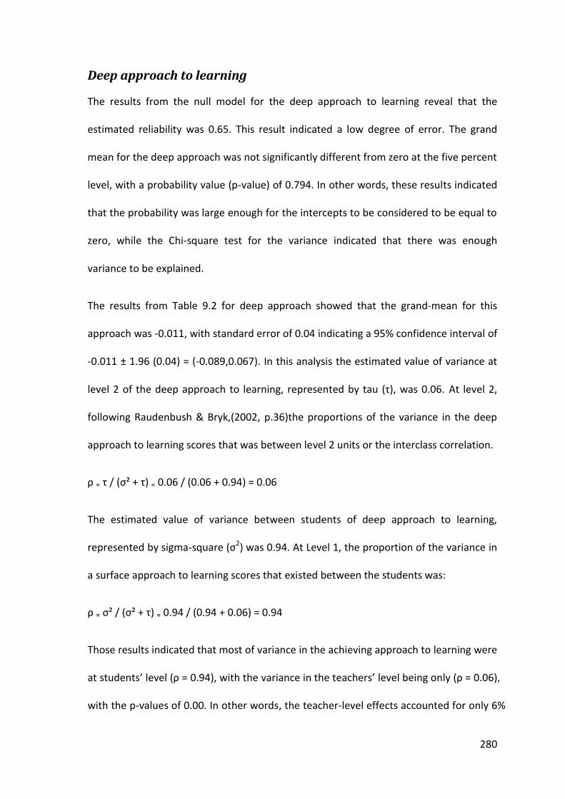
280

Deep approach to learning

The results from the null model for the deep approach to learning reveal that the

estimated reliability was 0.65. This result indicated a low degree of error. The grand

mean for the deep approach was not significantly different from zero at the five percent

level, with a probability value (p-value) of 0.794. In other words, these results indicated

that the probability was large enough for the intercepts to be considered to be equal to

zero, while the Chi-square test for the variance indicated that there was enough

variance to be explained.

The results from Table 9.2 for deep approach showed that the grand-mean for this

approach was -0.011, with standard error of 0.04 indicating a 95% confidence interval of

-0.011 ± 1.96 (0.04) = (-0.089,0.067). In this analysis the estimated value of variance at

level 2 of the deep approach to learning, represented by tau (τ), was 0.06. At level 2,

following Raudenbush & Bryk,(2002, p.36)the proportions of the variance in the deep

approach to learning scores that was between level 2 units or the interclass correlation.

ρ ₌ τ / (σ² + τ) ₌ 0.06 / (0.06 + 0.94) = 0.06

The estimated value of variance between students of deep approach to learning,

represented by sigma-square (σ2) was 0.94. At Level 1, the proportion of the variance in

a surface approach to learning scores that existed between the students was:

ρ ₌ σ² / (σ² + τ) ₌ 0.94 / (0.94 + 0.06) = 0.94

Those results indicated that most of variance in the achieving approach to learning were

at students’ level (ρ = 0.94), with the variance in the teachers’ level being only (ρ = 0.06),

with the p-values of 0.00. In other words, the teacher-level effects accounted for only 6%

281

of the total variance in deep approach to learning, while the remaining 94% was related

to between- student differences at the student level.

282

Table 9. 2 Null Models Results for Approaches to Learning

Outcome Reliability Estimate

Fixed Effect Coefficient Standard Error T-ratio df p-value

Surface Approach to learning (SA)

0.65 Intercept 1 for SA,B0

INTRCPT2, G00 0.007 0.04 0.18 51 0.862

Random Effect Standard Deviation Varian Component Df Chi-square p-value

Intercept 1 for SA,U0 Level 1, R

0.24949 0.96

0.06 0.94

51 156.86 0.00

Interclass Correlation Deviance

τ ₌ 0.06 σ² ₌ 0.94 ρ ₌ τ ⁄ (τ + σ²) ₌ 0.06 (6%)

4647.30 for 2 parameters

Deep Approach to learning (DA)

0.65 Intercept 1 for DA,B0

INTRCPT2, G00 -0.011 0.04 -0.26 51 0.794

Random Effect Standard Deviation Varian Component Df Chi-square p-value

Intercept 1 for DA,U0 Level 1, R

0.25131 0.96

0.06 0.94

51 166.40 0.00


τ ₌ 0.06 σ² ₌ 0. 94 ρ ₌ τ ⁄ (τ + σ²) ₌ 0.06 (6%)


Achieving Approach to learning (AA)

0.69 Intercept 1 for AA,B0

INTRCPT2, G00 -0.013 0.05 -0.30 51 0.761

Random Effect Standard Deviation Varian Component df Chi-square p-value

Intercept 1 for AA,U0 Level 1, R

0.27162 0.96

0.07 0.93

51 188.00 0.00


τ ₌ 0.07 σ² ₌ 0. 93 ρ ₌ τ ⁄ (τ + σ²) ₌ 0.07 (7%)


283

9.4 Final Results for the Approaches to Learning as the outcome variables

This section discusses on the final HLM results for the three learning approaches namely

surface, achieving and deep approaches. HLM version 6.0 was used to explore the

possible variables at Level 2 that could have significant effects. Step up procedure was

used until the final model, which with only the significant effects at both levels, was

obtained. The results of the fixed effect are presented first, followed by the explanation

of the results of variance. In all three models there was no cross-level interaction or

moderating effect on the variables.

Surface approach to learning

The final results for the surface approach to learning, which are summarized in Table 9.3

is specified by the following equation: format:

Level 1 Model

Yij = β0j + β1j *(SCHINESE) + β2j *(SCCP) + rij [9.4]

Level 2 Model

β0j = Υ00 + γ01* (TIN-FIELD) + U0j [9.5]

β1j = γ10 + U1j [9.6]

β2j = γ20 + U2j [9.7]

By substituting level-2 equations (Equations 9.4 to 9.7) into level-1, the final model is

represented by.

Yij = (Υ00 + γ01 (TIN-FIELD) + u0j) + (γ10 + u1j) (SCHINESE) + (γ20 + u2j) (SCCP) +rij [9.8]

284

The final model as expressed in Equation 9.8 illustrates that the implementation of the

surface approach to learning was a function of the overall intercept (Υ00), three main

effects, and a random error (u0j + u1j (SCHINESE) + u2j (SCCP) + rj). The three main effects

were the direct effects from TIN-FIELD (teacher in-field/out-of-field) at level 2 and

SCHINESE and SCCP at level 1 (students’). There was no cross-level interaction or

moderating effect between level 1 and level 2 variables.

Table 9. 3 Final Model of Surface Approach to Learning

Final estimation of fixed effect (wt robust standard errors)

Fixed Effect Coefficient Standard Error T-ratio Approx. Df P-value

For INTRCPT2, B0 INTRCPT2, G00 0.23 0.05 4.63 50 0.000 TIN-FIELD, G01 -0.20 0.06 -3.61 50 0.001 For SCHINESE slope, B2 INTRCPT2, G10 -0.41 0.08 -5.12 51 0.000 For SCCP slop, B2 INTRCPT2, G20 0.13 0.04 3.23 51 0.003

Final estimation of variance components

Random Effect Standard Deviation

Variance Component

DF Chi-square P-value

INTRCPT1, U0 0.23 0.05 40 89.830 0.000 SCHINESE slope, U1 0.44 0.19 41 86.056 0.000 SCCP slope, U2 0.21 0.04 41 109.831 0.000 Level-1, R 0.91 0.83

Statistics for current covariance components model

Deviance 4511.31 Number of estimate parameter

7

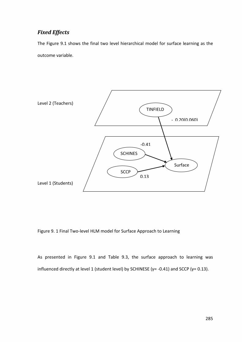
285

Fixed Effects

The Figure 9.1 shows the final two level hierarchical model for surface learning as the

outcome variable.

Level 2 (Teachers)

Level 1 (Students)

Figure 9. 1 Final Two-level HLM model for Surface Approach to Learning

As presented in Figure 9.1 and Table 9.3, the surface approach to learning was

influenced directly at level 1 (student level) by SCHINESE (γ= -0.41) and SCCP (γ= 0.13).

TINFIELD

TTTTINFI

ELD

SCHINES

E

SCHINES

E

SCHINES

E

SCHINES

E

SCCP

Surface

- 0.20(0.060)

0.13

(0.040)

-0.41

(0.080)

286

SCHINESE effects on Surface (-0.41/ 0.080)

Chinese ethnicity has a negative effect on the surface approach to learning (-0.41). This

negative effect indicates that the Chinese students were less likely to employ surface

approach in learning History in comparison to students of Malay, Indian and other

ethnicities in the History classroom.

CCP effects on Surface (0.13/ 0.040)

Students’ preferred History classroom climate had a positive effect on the surface

approaches to learning. The findings reveal that the students preferred personalized

and participation activities in the History classroom. This indicates that the more the

classroom climate is in line with what the students preferred the more students tend to

use surface approach.

Effects of TIN-FIELD on Surface (-0.20/ 0.060)

At the level 2 (teacher level), only one variable had a direct effect on surface approach

to learning. The analysis shows that teacher INFIELD (γ = -0.20) had negative effects on

the surface approach to learning. This finding indicates that students in the classroom

taught by in-field History teachers are less likely to adopt a surface approach to learning.

Goodness-of-Fit, Variance Partitioning and Variance Explained

The proportions of variance explained by the final model of student and teacher levels

are presented in Table 9.4. The percentages of variance of scores at both levels were

the maximum amount of variance available at those levels that were subsequently

explained in the HLM analyses. The results indicated that most of the variance (94%)

was found between students and only 6% occurred between teachers. The final model

287

explained (12%) of the variance available at the level 1 and (17%) of variance at level 2.

Overall the total amount of variance explained by the final model was 12%.

Table 9. 4 Estimation of Variance Component and Explained Variance for Surface Approach to Learning

Estimation of variance component between:

Students Teachers

Number of cases 1653 52 Null Model 0.94 0.06 Final Two – level HLM Model 0.83 0.05

Variance at each level 0.94 0.06 0.06 + 0.94 0.06 + 0.94 = 94 % = 6 % Proposition of variance explained 0.94 – 0.83 0.06 – 0.05 By final Two - Level Model 0.94 0.06 = 12% = 17 % Overall variance explained (0.94 – 0.83) + (0.06 – 0.05)

(0.94 + 0.06) =12%

The final model’s goodness-of-fit, presented in Table 9.2 and 9.3, showed that the

deviance was reduced by 112.87, from 4624.18 in the null model to 4511.31 in the final

model, with an additional 2 degrees of freedom.

Deep approach to learning

The final results for the deep approach to learning are specified by the following

equations:

Level 1 Model

Yij = β0j + β1 *(SGDR) + β2j *(SCHINESE) + β3j *(SCCP) + β4j *(SCCA) + rij

[9.9]

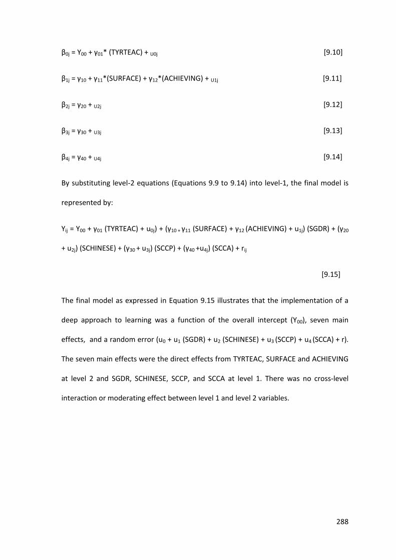
288

β0j = Υ00 + γ01* (TYRTEAC) + U0j [9.10]

β1j = γ10 + γ11*(SURFACE) + γ12*(ACHIEVING) + U1j [9.11]

β2j = γ20 + U2j [9.12]

β3j = γ30 + U3j [9.13]

β4j = γ40 + U4j [9.14]


represented by:

Yij = Υ00 + γ01 (TYRTEAC) + u0j) + (γ10 + γ11 (SURFACE) + γ12 (ACHIEVING) + u1j) (SGDR) + (γ20

+ u2j) (SCHINESE) + (γ30 + u3j) (SCCP) + (γ40 +u4j) (SCCA) + rij

[9.15]

The final model as expressed in Equation 9.15 illustrates that the implementation of a

deep approach to learning was a function of the overall intercept (Υ00), seven main

effects, and a random error (u0 + u1 (SGDR) + u2 (SCHINESE) + u3 (SCCP) + u4 (SCCA) + r).

The seven main effects were the direct effects from TYRTEAC, SURFACE and ACHIEVING

at level 2 and SGDR, SCHINESE, SCCP, and SCCA at level 1. There was no cross-level

interaction or moderating effect between level 1 and level 2 variables.

289

Table 9. 5 Final Model of Deep Approach to Learning



For INTRCPT1, B0 INTRCPT2, G00 -0.13 0.07 -0.84 50 0.071 TYRTEA G01 -0.005 0.001 -2.73 50 0.009 For SGDR slope, B1 INTRCPT2, G10 0.14 0.05 3.10 49 0.004 SURFACE G11 -0.11 0.04 -2.76 49 0.009 ACHIEVING G12 0.37 0.04 8.75 49 0.000 For SCHINESE slope,

B2

INTRCPT2, G20 -0.42 0.07 -5.72 51 0.000 For SCCP slope, B3 INTRCPT2, G30 0.25 0.03 7.55 51 0.000 For SCCP slope, B4 INTRCPT2, G40 0.14 0.02 6.51 51 0.000



Variance Component


INTRCPT1, U0 0.20 0.04 41 45.33 0.30 SGDR slope,

U1 0.15 0.02 39 46.90 0.18

SCHINESE slope,

U2 0.37 0.13 41 77.91 0.00

SCCP slope, U3 0.16 0.02 41 78.75 0.00 SCCA slope, U4 0.05 0.00 41 37.92 >.50 Level-1, R 0.83 0.70



16

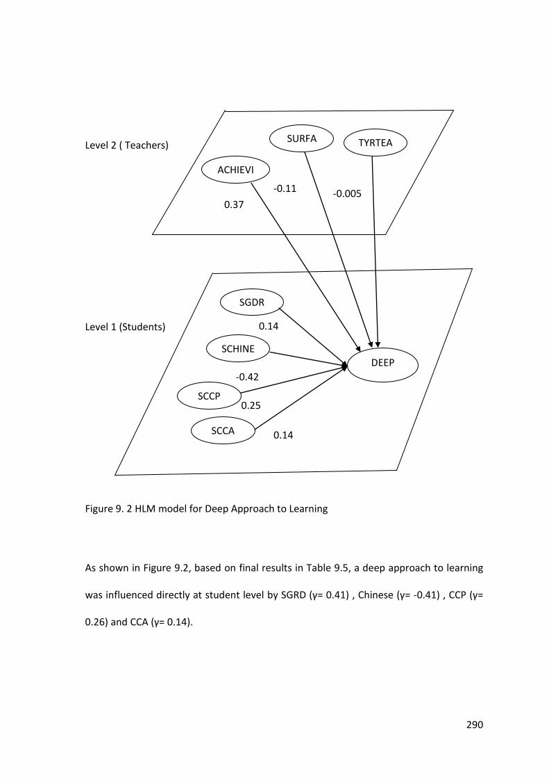
290

Level 2 ( Teachers)

Level 1 (Students)

Figure 9. 2 HLM model for Deep Approach to Learning

As shown in Figure 9.2, based on final results in Table 9.5, a deep approach to learning

was influenced directly at student level by SGRD (γ= 0.41) , Chinese (γ= -0.41) , CCP (γ=

0.26) and CCA (γ= 0.14).

ACHIEVI

NGG

SURFA

CE

TYRTEA

SGDR

SCHINE

SE

0.25

DEEP

SCCA

SCCP

0.14

(0.046)

20

(0.047)

0.14

(0.022)

(0.040.3

2

0.040.32

(0.046)

0.32

(0.046)

6)

-0.42

(0.070.04

0.32

0.040.32

(0.046)

0.32

(0.046)

6)

0.37

(0.045)

20

(0.047)

-0.11

(0.040)

20 (0.047)

0.20

-0.005

(0.001)

20 (0.047)

0.20

291

SGDR effects on DEEP

In term of students’ gender SGDR (0.41/ 0.045), the result indicates that the female

students were more likely to adopt a deep learning approach compared to male

students.

SCHINESE effects on DEEP

In term of the students’ ethnicity, Chinese students showed direct negative effects

(-0.42/00.71) on the deep approach to learning. This result indicated that Chinese

students were less likely to employ deep approach for the learning of History than

students of Malay, Indian and Other ethnicities.

CCP effects on DEEP and CCA effects on DEEP

Students’ preferred History classroom climate (CCP) (0.25/ 0.033) and actual classroom

climate (CCA) (0.14/ 0.022) both had a positive effect on the deep approach to learning.

This suggested that the more the classroom climate was in line with what the students

preferred and what they actually experienced, the more likely the students were to use

a deep approach to learning.

The HLM analyses also indicated that all the variables at the student level were

significant at p = 0.004 for (students’ gender) and, p = 0.000 for (ethnicity, CCP and CCA).

Overall, these findings highlight that both actual and preferred classroom environments

as well as, students’ gender and ethnicity had an important influence on the deep

learning approach.

At the teachers’ level, a direct influence on deep approach to learning came from three

factors TYRTEA (γ= -0.005), SURFACE (γ= -0.11) and ACHIEVING (γ= 0.38).

292

TYRTEA effects on DEEP

The results shows years of teaching (teacher experience) had a direct negative effect

(-0.005/ 0.002) on deep approach to learning. This indicated that students under

teachers who had more experience were less likely to adopt deep approach compared

to those under novice History teachers. Students under the novice History teachers

were more likely to employ deep approach to learning in the History classroom.

SURFACE effects on DEEP

In addition, students in classrooms, where, on average students used a surface

approach to learning (-0.11/ 0.038), were less likely to adopt a deep approach.

ACHIEVING effects on DEEP

In contrast, students in classrooms where, on average, students employed and

achieving approach to learning were more likely to use a Deep approach to learning

History (0.38/ 0.043).

The impacts for TYRTEA (-0.005) and SURFACE (-0.11) were small compared to

ACHIEVING (0.38). Furthermore, all the variables at the teacher level were substantially

significant at p = 0.009 for TYRTEA and for SURFACE, and p = 0.000 for ACHIEVING. In

summary, these teachers variables indicated that the teachers’ experience and

approaches toward teaching and learning History effected whether students adopted a

deep approach to learning History.


The proportions of variance in the final model at Level 1 and Level 2 are presented in

Table 9.6 HLM analysis demonstrated that the percentage of variance of scores at the

students’ and teachers’ levels of the hierarchy were the maximum amount of variance

293

available at those levels. Based on the results in Table 9.6, the total amount of variance

explained by the final model was 25%. Most of the variance (94%) was found between

students, while 6% occurred at teachers’ level. The final model explained (23%) of the

variance available at the level 1 and (33%) of variance at teachers’ level.

Table 9. 6 Estimation of Variance Component and Explained Variance for Deep Approach to Learning


Students Teachers


Variance at each level 0.93 0.06 0.06 + 0.93 0.06 + 0.93 = 94 % = 6 % Proposition of variance explained 0.93 – 0.70 0.06 – 0.04 By final Two - Level Model 0.93 0.06 = 23% = 33 % Overall variance explained (0.93 – 0.70) + (0.06 – 0.04)

(0.93 + 0.06) =25%

The final model’s goodness-of-fit as, presented in Tables 9.2 and 9.5 showed that, the



Achieving approach to learning

The final result for the achieving approach to learning is specified by the following

equation: format:

Level 1 Model

Yij = β0j + β1j *(SGDR) + β2j *(SMALAY) + β3j *(SCHINESE) + β4j *(SCCP) + β5j *(SCCA) + rij

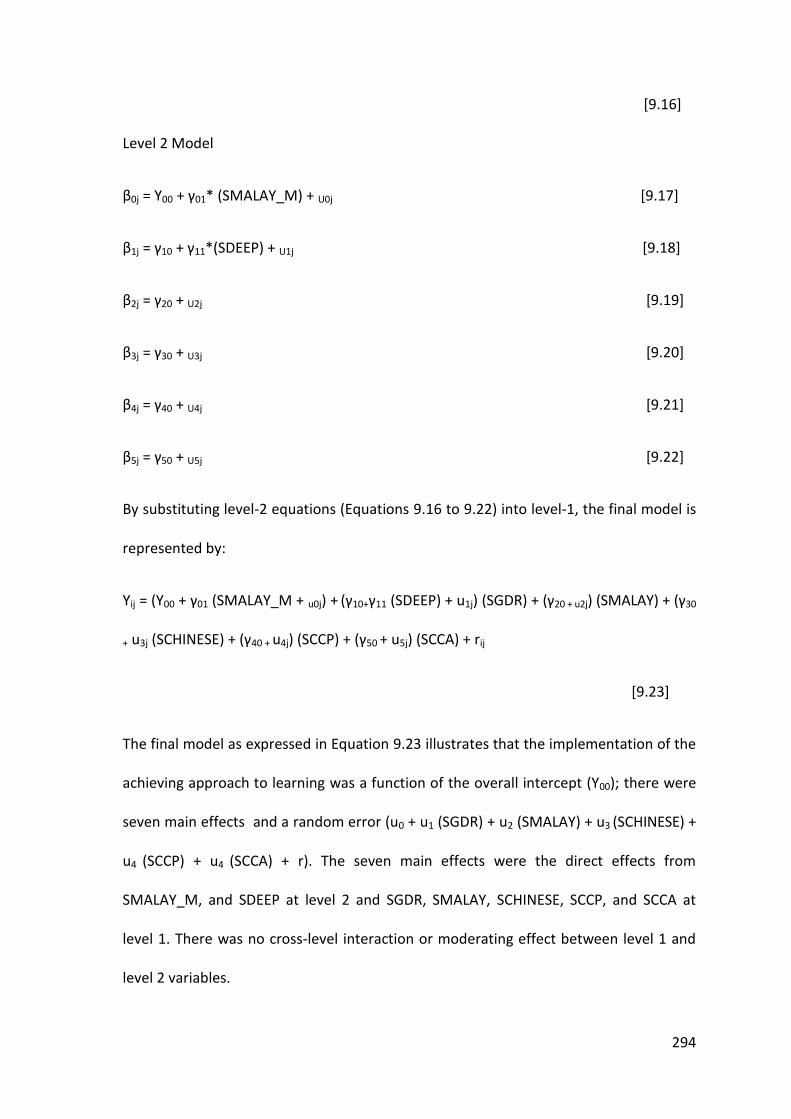
294

[9.16]

Level 2 Model

β0j = Υ00 + γ01* (SMALAY_M) + U0j [9.17]

β1j = γ10 + γ11*(SDEEP) + U1j [9.18]

β2j = γ20 + U2j [9.19]

β3j = γ30 + U3j [9.20]

β4j = γ40 + U4j [9.21]

β5j = γ50 + U5j [9.22]


represented by:

Yij = (Υ00 + γ01 (SMALAY_M + u0j) + (γ10+γ11 (SDEEP) + u1j) (SGDR) + (γ20 + u2j) (SMALAY) + (γ30

+ u3j (SCHINESE) + (γ40 + u4j) (SCCP) + (γ50 + u5j) (SCCA) + rij

[9.23]

The final model as expressed in Equation 9.23 illustrates that the implementation of the

achieving approach to learning was a function of the overall intercept (Υ00); there were

seven main effects and a random error (u0 + u1 (SGDR) + u2 (SMALAY) + u3 (SCHINESE) +

u4 (SCCP) + u4 (SCCA) + r). The seven main effects were the direct effects from

SMALAY_M, and SDEEP at level 2 and SGDR, SMALAY, SCHINESE, SCCP, and SCCA at

level 1. There was no cross-level interaction or moderating effect between level 1 and

level 2 variables.

295

Table 9. 7 Final Model of Achieving Approach to Learning



For INTRCPT1, B0 INTRCPT2, G00 -0.22 0.08 -2.77 50 0.008 SMALAY_M G01 -0.23 0.09 -2.34 50 0.023 For SGDR slope, B1 INTRCPT2, G10 0.20 0.05 4.10 50 0.000 SDEEP G11 0.36 0.04 8.63 50 0.000 For SMALAY slope, B2 INTRCPT2, G20 0.18 0.08 2.20 51 0.032 For SCHINESE slope, B3 INTRCPT2, G30 -0.32 0.08 -4.19 51 0.000 For SCCPAM slope, B4 INTRCPT2, G40 0.26 0.04 7.18 51 0.000 For SCCPAM slope, B5 INTRCPT2, G50 0.13 0.02 5.60 51 0.000



Variance Component


INTRCPT1, U0 0.20 0.04 32 32.57 0.44 SGDR slope, U1 0.18 0.03 32 44.51 0.07 SMALAY U2 0.22 0.05 33 38.46 0.24 SCHINESE slope, U3 0.28 0.08 33 35.77 0.34 SCCP slope, U4 0.19 0.04 33 70.30 0.00 SCCA slope, U5 0.07 0.004 33 35.26 0.40 Level-1, R 0.81 0.70


Deviance 4127.11

Number of estimate parameter

22

296

-0.32

0.13

(0.022)

(0.040.3

2

0.040.32

(0.046)

0.32

(0.046)

6)

SGDR

SMALAY

ACHIEVING

SCCP

SCHINESE

0.19

(0.047)

20

(0.047) 0.26

(0.036)

(0.040.3

2

0.040.32

(0.046)

0.32

(0.046)

6)

0.18

(0.081)

(0.040.32

0.040.32

(0.046)

0.32

(0.046)

6)

0.36

(0.041)

20 (0.047)

0.20

0.23

(0.096)

20 (0.047)

0.20

SCCA

SDEEP SMALAY_M

M

Level 2 (Teachers)

Level 1(Students)

Figure 9. 3 HLM model for Achieving Approach to Learning

The final results in Table 9.7, as presented in Figure 9.3, revealed that an acheiving

approach to learning was influenced directly at student level by SGRD (β= 0.19) , SMalay

(β= -0.18), SChinese (β= -0.32) , CCP (β= 0.26) and CCA (β= 0.13).

SGDR had a positive effect on Achieving approach to learning (0.19/0.047) This result

indicated that the female students were more likely to employ the achieving approach

to learning compared to male students.

297

SMALAY effects on Achieving approach to learning

The results revealed that Malay student (SMALAY) had a positive effect (0.18/0.081)

on the achieving approach to learning. This result indicates that the Malay students

were more likely adopt the achieving learning approach compared to student of Chinese,

Indian and Other ethnicities.

SCHINESE effects on Achieving approach to learning

Students’ of Chinese ethnicity had a negative direct influence(-0.32/0.077) on the

achieving approach. The results reveal that Chinese students’were less likely to employ

the achieving approach compared to non-Chinese students’.

CCP and CCA effects on Achieving approach to learning

Students’ preferred History classroom climate (CCP) (0.26/0.036) and actual classroom

climate (CCA) (0.13/0.022) had a positive effects on the achieving approach to learning.

These indicated that the more the classroom climate was in line with what the students

preferred and what they actually experienced the more likely they were to use the

achieving approach to learning.

The HLM analyses also indicated that all the variables at the student level were

significant at p = 0.000 for (SGDR, SCHINESE, CCP and CCA), p = 0.032 for (SMALAY).

Overall these findings highlighted that both actual and preferred History classroom

climates as well as, students’ gender and ethnicity influenced students’ use of an

achieving learning approach in the History classroom.

298

At level 2 (the teacher level), there were two variables which had direct effects on the

achieving approach to learning: SMALAY_M (γ= 0.23) and DEEP (γ= 0.36). The results

show that both variables had positive influence on the achieving approach.

SMALAY_M effects on Achieving approach to learning

The result showed the proportion of Malay students (SMALAY_M) in the classroom had

a positive effect (0.23/0.096) on the achieving approach to learning. This indicates that

the students in a classroom that had higher proposition of Malay students were likely to

adopt an achieving approach to learning.

SDEEP effects on Achieving approach to learning

These results showed that SDEEP had a direct positive effects (0.36/0.041) on the

achieving approach to learning. This indicated that, students in the classroom that had

higher proportion of students adopting deep approach to learning were more likely to

use achieving approach to learning in the History classroom.


The proportions of variance explained by the final model at students and teachers level

are presented in Table 9.8. The percentages of variance of scores at both levels were

the maximum amounts of variance available at those levels that were subsequently

explained in the HLM analyses. The results indicate that most of the variance (93%) was

found between students’ variable and 7% occurred between teachers’ variables. The

final model explained (27%) of the variance available at the level 1 and (43%) of

variance at teachers’ level. Overall, the total amount of variance explained by the final

model was 28%.

299

Table 9. 8 Estimation of Variance Component and Explained Variance for Achieving Approach to Learning


Students Teachers


Variance at each level 0.92 0.07 0.07 + 0.92 0.07 + 0.93 = 93% = 7% Proposition of variance explained 0.92 – 0.67 0.07 – 0.04 By final Two - Level Model 0.92 0.07 = 27 % = 43 % Overall variance explained (0.92 – 0.67) + (0.07 – 0.04)

(0.92 + 0.07) = 28 %

In the final estimations goodness-of-fit model, presented in Table 9.7 and 9.8, the


model, with an additional 20 of degrees of freedom.

9.5 HLM finding for the Students’ Learning Outcome as the outcome variable

This section discusses the result of HLM-two level analysis of the student learning

outcome (SOUTCOME). The discussion is focussed on the effects of the students’ and

teachers’ characteristics on students’ learning outcome.

Table 9.9 presents the results of the null model for student learning outcomes

(SOUTCOMES). The null model was tested to determine if HLM were necessary for the

outcome specified.

300

Table 9. 9 Null Model Results for the Students’ Learning Outcomes (SOUTCOME)

Outcome Reliability Estimate

Fixed Effect Coefficient Standard Error

T-ratio df p-value

Student Learning Outcome (SOUTCOME)

0.76 Intercept 1 for SOUTCOME,B0

INTRCPT2, G00 -0.016 0.05 -0.31 51 0.753


Varian Component

df Chi-square

p-value

Intercept 1 for SOUTCOME,U0 Level 1, R

0.32666 0.94

0.10 0.89

51 254.61 0.000

Interclass

Correlation Deviance

τ ₌ 0.10 σ² ₌ 0.89 ρ ₌ τ ⁄ (τ + σ²) ₌ 0.10 (10%)


The reliability estimate of the null model of the students’ learning outcome was high at

0.76. The grand mean of students learning outcome (SOUTCOME) was not significantly

different from zero at the five percent level with the probability value (p-value) of 0.761.

This result indicated that the p-value was large enough for the intercepts to be

considered equal to zero. Furthermore, the chi-square test for variance indicated that

there was enough variance to be explained. Thus, this result indicated that it was worth

carrying out a two-level HLM analysis.

The grand-mean result was -0.016, with the standard error of 0.05, indicating a 95%

confidence interval of -0.016 ± 1.96 (0.04) = (-0.0944, 0.0624). The estimated variance at

level 2 of the SOUTCOME, represented by tau (τ), was 0.10. The estimated value of

variance between students of surface approach to learning, represented by sigma-

square (σ2) was 0.89.

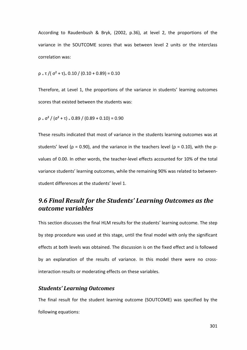
301

According to Raudenbush & Bryk, (2002, p.36), at level 2, the proportions of the

variance in the SOUTCOME scores that was between level 2 units or the interclass

correlation was:

ρ ₌ τ /( σ² + τ)₌ 0.10 / (0.10 + 0.89) = 0.10

Therefore, at Level 1, the proportions of the variance in students’ learning outcomes

scores that existed between the students was:

ρ ₌ σ² / (σ² + τ) ₌ 0.89 / (0.89 + 0.10) = 0.90

These results indicated that most of variance in the students learning outcomes was at

students’ level (ρ = 0.90), and the variance in the teachers level (ρ = 0.10), with the p-

values of 0.00. In other words, the teacher-level effects accounted for 10% of the total

variance students’ learning outcomes, while the remaining 90% was related to between-

student differences at the students’ level 1.

9.6 Final Result for the Students’ Learning Outcomes as the outcome variables

This section discusses the final HLM results for the students’ learning outcome. The step

by step procedure was used at this stage, until the final model with only the significant

effects at both levels was obtained. The discussion is on the fixed effect and is followed

by an explanation of the results of variance. In this model there were no cross-

interaction results or moderating effects on these variables.

Students’ Learning Outcomes

The final result for the student learning outcome (SOUTCOME) was specified by the

following equations:

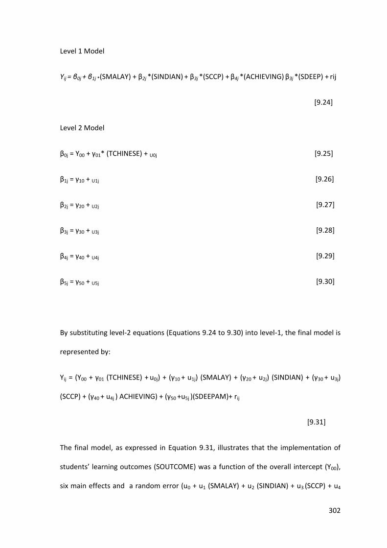
302

Level 1 Model

Yij = β0j + β1j *(SMALAY) + β2j *(SINDIAN) + β3j *(SCCP) + β4j *(ACHIEVING) β3j *(SDEEP) + rij

[9.24]

Level 2 Model

β0j = Υ00 + γ01* (TCHINESE) + U0j [9.25]

β1j = γ10 + U1j [9.26]

β2j = γ20 + U2j [9.27]

β3j = γ30 + U3j [9.28]

β4j = γ40 + U4j [9.29]

β5j = γ50 + U5j [9.30]


represented by:

Yij = (Υ00 + γ01 (TCHINESE) + u0j) + (γ10 + u1j) (SMALAY) + (γ20 + u2j) (SINDIAN) + (γ30 + u3j)

(SCCP) + (γ40 + u4j ) ACHIEVING) + (γ50 +u5j )(SDEEPAM)+ rij

[9.31]

The final model, as expressed in Equation 9.31, illustrates that the implementation of

students’ learning outcomes (SOUTCOME) was a function of the overall intercept (Υ00),

six main effects and a random error (u0 + u1 (SMALAY) + u2 (SINDIAN) + u3 (SCCP) + u4

303

(ACHIEVING) + u5 (SDEEP) + r). The six main effects were the direct effects from

TCHINESE at level 2 and SMALAY, SINDIAN, SCCP, ACHIEVING and SDEEPAM, at level 1.

There were no cross-level interactions or moderating effects between level 1 and level 2

variables.

Table 9. 10 Final Model of Students’ Learning Outcomes (SOUTCOME)



For INTRCPT1, B0 INTRCPT2, G00 -0.30 0.04 -7.73 50 0.000 TCHINESE G01 -0.29 0.08 3.85 50 0.000 For SMALAY slope, B1 INTRCPT2, G10 0.38 0.05 8.21 51 0.000 For SINDIAN slope, B2 INTRCPT2, G20 0.27 0.08 3.56 51 0.001 For SCCPAM slope, B3 INTRCPT2, G30 0.12 0.02 6.12 51 0.000 For ACHIEVING slope, B4 INTRCPT2, G40 0.34 0.06 5.74 51 0.000 For SDEEPAM slope, B5 INTRCPT2, G50 0.23 0.06 4.10 51 0.000



Variance Component


INTRCPT1, U0 0.10 0.01 29 27.63 >.50 SMALAY slope, U1 0.13 0.02 30 32.62 0.34 SINDIAN slope, U2 0.12 0.02 30 20.91 >.50 SCCPAM slope, U3 0.05 0.002 30 34.94 0.24 ACHIEVING slope, U4 0.18 0.03 30 33.22 0.31 SDEEPAM slope, U5 0.16 0.03 30 27.24 >.50 Level-1, R 0.70 0.49



22

304

TCHINESE

0.29

(0.075)

SOUTCOME

SPEAcgea

SPEACH

SINDIAN

SCCP

ACHIEVI

NG SDEEP

0.38

(0.046)

0.27

(0.076) 0.12

(0.019)

0.23

(0.057)

0.34

SMALAY

Level 2 (Teachers)

Level 1 (Students)

Figure 9. 4 HLM model for Students’ Learning Outcomes (SOUTCOME)

Table 9.9 and Figure 9.4 show that students’ learning outcomes was influenced directly

at student level by SMALAY (β= 0.37), SINDIAN (β= 0.27), SCCP (β= 0.12), ACHIEVING (β=

0.34) and SDEEP (β= 0.23).

SMALAY effects on Studens’ Learning Outcomes

The results show that being a Malay student had a positive direct effect (0.37/0.046) on

student learning outcomes (SOUTCOME). This positive result indicated that Malay

students (SMALAY) were more likely to perceive that the History teaching outcome had

achieved its intended outcomes as stated in the curriculum.

305

SINDIAN effects on Students’ Learning Outcomes

Similar results were evident for the Indian students (SINDIAN). This result show a

positive direct effect (0.27/ 0.076) which revealed that Indian students were more likely

to perceive that History teaching had accomplished its intended outcome as stated in

the History curriculum.

CCP effects on Students Learning Outcomes

For students’ preferred History classroom climate (CCP) the results revealed a positive

effect (0.12/0.019) on students’ learning outcomes. This indicates that the preferred

History classroom climate had positive influence on the students’ learning outcomes.

Student who perceived a higher level of CCP in terms of personalised and participatory

activities in the preferred History classroom perceived that History teaching had

managed to achieve its learning outcomes as stated in the History curriculum.

ACHIEVING effects on Students’ Learning Outcomes

Students who adopted achieving learning approaches had positive direct effects (0.34/

0.059) on students’ learning outcome. The analysis showed that students who adopted

the achieving approach to learning were more likely to perceive that the History teacher

had fulfilled the History learning objective as stated in the curriculum.

DEEP effects on Students’ Learning Outcomes

Similar results were evident for students who employed deep approach to learning.

Students who employed a deep approach (0.23/ 0.057) were more likely to perceive

that History teachers had achieved the learning outcomes as stated in the History

curriculum.

306

At level-2 the (teacher level), only one variable had positive directs effects on the

students’ learning outcomes; TCHINESE (β= 0.29). The result indicated that in a

classroom with a higher proportion of Chinese students, students generally were more

likely to perceive that History teachers had achieved their teaching goals as stated in the

History curriculum.


The proportions of variance explained by the final model at the students’ and teachers’

levels are presented in Table 9.11. The percentage of variance of scores at both levels

were the maximum amounts of variance available at those levels that were

subsequently explained in the HLM analyses. The results indicated that most of the

variance (89%) was found between students’ variables and only 11% occurred between

teachers’ variables. The final model explained (5%) of the variance available at the level

1 and (91%) of variance at teachers level. Overall the total amount of variance explained

by the final model was 49%.

307

Table 9. 11 Estimation of Variance Component and Explained Variance for Student Learning Outcome


Students Teachers


Variance at each level 0.90 0.11 0.12 + 0.89 0.11 + 0.89 = 89 % = 11 % Proposition of variance explained 0.89 – 0.50 0.11 – 0.01 By final Two - Level Model 0.89 0.11 = 5 % = 91 % Overall variance explained (0.89 – 0.50) + (0.11 – 0.01)

(0.89 + 0.11) = 49 %

The final model’s goodness-of-fit, presented in Tables 9.10 and 9.11, showed that, the



9.7 Summary of the HLM findings

This chapter has presented the final two-level hierarchical linear models for the learning

approaches models, surface, deep and achieving,as well as the learning outcomes,in

relation to the students’ and teachers’ characteristics. Overall, four models were tested

in the HLM analysis: (a) surface, (b) deep, (c) achieving, and (d) student learning

outcomes. However, in this analysis there was no cross-level interaction or moderating

effects on the direct effects of the variables used in this analysis. The findings are based

on the direct effects that emerged from the two-level hierarchical linear models.

308

The null model was carried out as the beginning step of the HLM analysis to estimate

the amount of variance available at the two levels. The same procedure was followed

for each of the final models.

Since the HLM results did not show any cross-level interaction or moderating effects,

the HLM findings only discussed the direct effects made evident between Level-1 and

Level-2. The final model of surface approach to learning indicated that two of Level-1

variables, namely Chinese students (SCHINESE) and classroom climate preferred (CCP),

and as well as one variable at Level-2: out-of-field/in-field History teachers (TINFIELD)

influenced directly the students’ adoption of the Surface learning approach.

The final model findings of the deep approach to learning indicated that three Level-1

variables e.g.: teachers’ years of teaching (TYRRTEA), surface (SURFACE) and Achieving

(ACHIEVING) approaches to learning, as well as four variables at Level-2, namely

students’ gender (SGDR), Chinese students (SCHINESE), classroom climate preferred

(SCCP) and classroom climate actual (SCCA) directly influenced students’ use of deep

approach to learning.

The Achieving approach to learning final models revealed that two of the Level- 2

variables, SMALAY and SDEEP, and five Level-1 variables SGDR, SMALAY, SCHINESE,

SCCP and SCCA, showed direct influences on students’ adoption of the achieving

approach to learning.

The final model of the studens’ learning outcomes (SOUTCOME) indicated that one

variable from Level-1, TCHINESE and five variables from Level-2: SMALAY, SINDIAN,

SCCP, ACHIEVING, and SDEEP had direct effects on the SOUTCOME.

309

Overall, the HLM analyses revealed number of important findings:

1) The effects of the TINFIELD History teachers (y= -0.20) on surface learning approach.

This finding indicated that students’ in the clases of in-field History teachers were less

likely to employ the surface approach in comparison to students in out-of-field History

teaches’ classes. The results showed that the Chinese students were less likely to adopt

the surface approach (-0.41) to learning compared to non-Chinese students.

Furthermore, the results revealed that SCCP had a positive effect (y= 0.13) on the

surface learning approach, in that students in a History classroom which was close to

their preferred climate were more likely to employ a surface approach to learning

2) The results on Deep Approach to learning at students’ level showed that girls (y= 0.41)

were more likely to adopt a Deep approach to learning in comparisons to boys.

Compared to the results on the surface approach to learning, Chinese students (y = -

0.42) were less likely to adopt less a deep approach to learning compared to students of

Malay, Indian and Others ethnicities. The findings in relation to preferred and actual

classroom climates, SCCP (y = 0.25) and SCCA (y= 0.14). This indicated that the more the

classroom climate was in line with what the students preferred and what they actually

experienced, the more likely they were to use the deep approach to learning History in

the classroom.

At the teacher level, the result revealed that TYRTEA (y = - 0.005), teachers who had

more experience, were less likely to encourage a deep approach compared to novice

History teachers. Furthermore, Surface approach to learning (y = -0.11) show a negative

effect on the DEEP approach to learning. This suggested that the students in a

classroom where on average more students used the surface approach to learning,

310

were less likely to employ a Deep approach. In contrast, the positive effects of achieving

(y= 0.38) shows that in a classroom that had a high proportion of students who used

the achieving approach to learning, students generally were more likely to adopt Deep

approach to learning in learning History classroom.

3) The finding on Achieving approach to learning showed the effect of student gender.

The results indicated that girls (y= 0.19) were more likely to adopt an Achieving learning

approach compared to boys. Malay students (β= 0.18) were also more likely adopt the

Achieving learning approach in comparison to non-Malay students. On the other hand,

the result for Chinese students (β = -0.32) indicated that they were less likely to employ

Achieving approach to learning compared to students of Malay, Indian and Others

ethnicities. Classroom climate, both SCCP (y = 0.26) and SCCA (y= 0.13), had positive

influences on the Achieving approach to learning. This suggested that the more the

classroom climate was in line with what the students preferred and what they actually

experienced, the more they were likely to adopt the Achieving approach in learning

History

At the teacher level, the results showed that SDEEP (y = 0.36) and SMALAY_M (0.23) had

positive direct effects on the Achieving approach to learning. This showed that students

in a classroom that had a high proportion of Malay students were more likely to adopt

the Achieving approach to learning. Additionally, the results also indicated that in a

classroom that had more students employing the Deep approach to learning (y =0.36),

the more likely it was that students would use the Achieving approach to learning in the

History classroom

311

4)The findings on Students’ learning outcomes (SOUTCOME), showed positive effects

for Malay students (β = 0.38) and Indian students (β= 0.27). These figures indicated that

Malay students (SMALAY) and Indian students (SINDIAN) were more likely to perceive

that the History teacher had accomplished the intended learning outcomes as stated in

the History curriculum in comparison to students of other ethnicities. Similar results

were found for students who adopted Achieving approach to learning (y = 0.34). They

perceived that the History teacher had achieved the outcome in teaching History in

comparison to those students with a DEEP (y = 0.23) learning approach. For the

preferred History classroom climate (SCCP), the results showed that SCCP had a low

positive (y = 0.12) direct effect on the SOUTCOME. This positive effect indicated that

student who perceived a higher level of SCCP were more likely to perceive that History

teachers had accomplished the History learning objectives as stated in the History

curriculum. At the teachers’ level, the results showed that TCHINESE had positive effect

(β= 0.29) on students learning outcomes. This indicated that in a classroom that had

higher proportion of Chinese students, students generally were more likely to perceive

that the History teachers had achieved the History learning outcomes.

In conclusion, although there were no cross-level interactions or moderating effects

found in the models discussed, the two-level HLM analysis used in this study provided

general support for student learning approaches, namely surface, deep and achieving.

The findings revealed that those variables did effect the students’ learning outcomes.

Moreover, HLM analyses findings indicated the direct influence of the variables

discussed at both student and teacher levels in a way that confirmed and strengthened

the findings in the previous chapters. These HLM results provided some evidence

312

concerning the comparative effects of out-of-field and in-field teachers on secondary

History classrooms in Malaysia.

Probably, the most important finding to emerge from the HLM analysis was the

comparatively small effects reported for the level 2 variables, Teacher qualifications in

History (whether out-of-field or in-field) and Teacher Experience, (which was closely

linked to qualifications) did not emerge as important factors in the learning outcomes

of Malaysian History classrooms. The in-field qualification did occur once as a negative

effect on students’ adoption of surface approaches to learning, while Teachers’

Experience had a small negative effect on students’ adoption of deep approaches to

learning. The implications of these findings are considered in the concluding chapter

that follows.

313

Chapter 10 Discussion and Conclusions ________________________________________________________________________

10.1 Introduction

The final chapter discusses the findings of this investigation into the phenomenon of

out-of-field History Teaching in Malaysian secondary schools. It begins by summarizing

the aims and design of the study and reporting the findings which directly answered the

original research questions. Subsequent sections consider the implications of the

findings for secondary History classrooms in Malaysia, the need for a replication of the

investigation and recommendations for future research.

10.2 Design of the study

The study set out to investigate the impact of out-of-field History teachers on the

teaching and learning processes in Form Four secondary school History classrooms in

Malaysia. Although the phenomenon of out-of-field teaching can be found in many

countries, this present research focussed on three broad questions related to History

teaching in Malaysian secondary schools. As outlined in Chapter 1, these were:

(a) Are there any differences between out-of-field and in-field History teachers?

(b) What are the impacts of teacher qualifications (in-field and out-of-field) on the

History teaching and learning process at the classroom and student level?

(c) How do the teacher qualifications (in-field and out-of-field) interact with other

factors in influencing the teaching and learning process in the History classroom?

In the course of reviewing previous research in the area of in-field and out-of-field

teachers in the classroom learning, a number of teacher and student factors, which

314

could influence the learning process in the History classroom were identified and a

theoretical framework, based on Biggs’s 3P Model of students’ learning, was developed.

To gather data related to the variables identified in this framework, the researcher

prepared a set of teachers’ questionnaires which incorporated three scales. These were

the Teachers’ Conceptions of Teaching by Gao & Watkins (2002), the Approaches to

Teaching Instruments (ATI) by Trigwell, Prosser and Ginns (2005), and a History Teaching

Method questionnaire which was developed by the researcher. Similarly, there was a

set of students’ questionnaires, incorporating three scales: the Individualised Classroom

Environment Questionnaire (ICEQ) by Fraser (1990), the Biggs’s Learning Process

Questionnaire (LPQ) by Biggs (1987), and a questionnaire on Students’ Perceptions of

History Learning developed by the researcher. A total of 52 Form Four History teachers

from Kuala Lumpur secondary schools completed the teacher questionnaires and 1653

students, taught by these teachers, completed the students’ questionnaires.

In the analysis of the data, the Confirmatory Factor Analysis was used to check the

validity and consistency of the questionnaires. The validity of the teacher and student

questionnaires were discussed in Chapters 4 and 5 respectively. In order to examine the

relationships between the latent and manifest variables in the measurement models

and between the latent variables in the structural model, the partial least square (PLS)

path analysis technique was employed (see Chapters 7 & 8). Since this study involved

two levels of data, teacher and student, Hierarchical Linear Modelling (HLM) was

employed to examine effects at the two levels, as well as the interaction between the

effects at these levels (see Chapter 9).

315

10.3 Summary of the findings

This section presents the findings of the study based on the research questions

advanced in Chapter 1. Research question 1 was answered on the basis of the t-test

analyses reported in Chapter 6, whilst the answers to research questions 2 and 3 were

based on the PLS and HLM analyses in Chapters 7, 8 and 9.

Research Question 1

Are there any differences between out-of-field and in-field History teachers?

The t-test analysis (see Chapter 6) was used to examine the differences between out-of-

field teachers and in-field teachers. On most of the variables tested, there were no

statistically significant differences between in-field and out-of-field History teachers in

Malaysia. The only four variables in which the differences proved significant were

teacher experience, the teaching conception of conduct guidance, the dimensions of

personalization, participation, independent and differentiation (see Chapter 4) in the

students’ preferred classroom climate, and the dimension of personalisation in the

students’ actual classroom environment.

In relation to teacher experience (measured in years of teaching) the results indicated

that out-of-field History teachers were less experienced compared to the in-field

teachers. Out-of-field History teachers had, an average of 7 years of service, compared

to 14 years for in-field teachers. The finding would seem to be the consistent with the

school context in Malaysia. As student numbers have increased, and schools have

needed more History teachers, there has been a tendency to make use of less

experienced members of staff as out-of-field history teachers. Staff members with more

316

experience are more likely to be teaching in the area of their training specialisation, in

this case upper level History.

Of the five dimensions of teachers’ teaching conceptions employed, only the conduct

guidance conception, which previous studies had identified as an important aim of

teaching (e.g. Goa & Watkins, 2001; Pratt 1992; Fox 1983), showed a significant

difference between in-field and out-of-field teachers. This result indicated that in-field

teachers, whom the previous results had shown to be the more experienced teachers,

were more likely to be committed to nurturing the personal conduct of their students

through their History teaching.

In terms of preferred classroom climate, there was a significant difference between

students of in-field teachers and those of out-of-field teachers on four out of the five

dimensions. This means that students under in-field teachers preferred classrooms

where they experienced investigation, personalisation, participation, and differentiation.

On the fifth dimension of independence there was no difference between the two

groups of students, suggesting that the authority of the teacher in the classroom was

recognised, whether they were fully qualified or not.

In the actual students’ classroom climate, out of the five dimensions used for this factor,

only personalisation showed any significant difference between students under the two

groups of teachers, with students of in-field teachers experiencing greater

personalisation. This result can be explained by the greater experience of in-field

teachers in the Malaysian context. In particular, they are more likely to have been

teaching longer in the same school and even to have taught the same class for two or

317

more years. They thus have had a greater opportunity to gain personal understanding of

the students they are teaching.

It is possible, that out-of-field teachers, who are younger and less experienced, may be

able to develop a more personalised dimension to their classrooms, as they gain more

familiarity with the History syllabus and get to know the students in their classes better.

An out-of-field teacher whose efforts are concentrated on subject content which is new

to them, has less time to focus on understanding students’ needs and interests. The

chance for professional development in the teaching of History may help them to

become more familiar with the content and assessment requirements, so that they are

able to direct more of their attention to the individual students in their class.

There were four variables which showed no significant difference on the t-test results in

this study, namely; teachers’ teaching approach, teaching methods, students’

approaches to learning, and learning outcomes. This is an important finding in that it

indicates not only that in-field and out-of-field teachers were using much the same

teaching approaches and methods, but also that the students under each group of

teachers were adopting similar approaches to learning and perceiving much the same

learning outcomes in their History classroom. These results can be seen to be consistent

with expectations that teachers in Malaysia follow the set of objectives and lesson plans

laid out in the History syllabus. In addition, out-of-field teachers are fully trained in

another area of specialization and thus can be expected to adopt their knowledge and

teaching skills to the teaching of History.

318

Research Question 2

What are the impacts of teachers’ qualifications (in-field and out-of-field) on the

History teaching and learning process at the classroom and student level?

PLS and HLM were used to address this research question which was related to the aim

of investigating how History teachers’ qualifications (whether in-field or out-of-field)

impacted directly on other factors to influence the learning outcomes in the History

classroom. For the teacher and student samples, the PLS (single-level) path analysis

indicated that there were five variables that showed direct (either positive or negative)

relationships with teachers’ qualifications (in-field or out-of-field).

One of these variables was teacher age. The results showed that the teachers’ age was

strongly associated with their type of qualification, with older teachers being, in general,

more qualified in History than their younger counterparts. In addition to being better

qualified to teach History, these older teachers were, as could be expected, also more

experienced in teaching the subject.

In relation to Classroom Climate Preferred students of in-field History teachers were

more likely to prefer a classroom environment which was personalized, participatory

and focused on investigating. For the Classroom Climate Actual, students of in-field

History teachers (who were more likely to be older teachers) tended to experience their

actual classroom climate as independent, participatory, and differentiated.

An indirect relationship was also found between in-field teachers and student learning

outcomes through the teacher experience factor. Students taught by experienced

History teachers (mainly in-field teachers) were more likely to show a higher level of

appreciation of the History syllabus objectives and the way learning History fostered

319

their learning of moral values. They also showed more appreciation of their increased

maturity and ability to think individually and the efforts and the contributions of

individuals who have struggled for the independence and development of the country,

and for the community in general. This result is consistent with expectations that in-

field teachers would have greater understanding of the History syllabus and its

objectives than out-of-field teachers, partly because of their training and partly because

of their greater overall experience of teaching History.

The results of the PLSPATH analyses showed that teacher qualifications (out-of-field and

in-field) had no direct relationship either to student learning approaches or to student

History learning outcomes. This is consistent with the t-test results which showed no

difference in teaching methods and approaches in the classroom between out-of-field

and in-field History teachers. The overall implication is that there was no difference

between out-of-field and in-field teachers in their impact on their students’ learning

approaches and History learning outcomes in Malaysian classrooms.

Research Question 3

How do the teacher qualifications (in-field and out-of-field) interact with other

factors in influencing the teaching and learning process in the History

classroom?

Path model analysis and Hierarchical Linear Modeling were used to examine the inter-

relationships between teachers’ qualifications (in-field and out-of-field) and other

teaching and learning factors at both classroom and student levels. It had been argued

that variables such as teachers’ teaching conceptions, approaches, and methods would

320

be expected to influence the climate of the classroom which in turn would have some

impact on students’ approaches to learning in the History classroom.

The results indicated that older History teachers were more likely to adopt effective and

active teaching methods in the classroom. Moreover, they were also more likely to have

a higher level of conceptions of teaching in the History classroom. In turn, the teaching

methods they employed influenced the actual classroom climate.

In terms of student approaches to learning, the variable of teachers’ qualifications was

found to have no direct effect on any of the three student approaches to learning

(Surface, Achieving and Deep). However, out-of-field teacher qualifications had a small

indirect, but negative effect on the Achieving learning approach through classroom

climate actual.

In relation to the Deep approach to learning, four variables at the student level namely,

student gender, Chinese student ethnicity, classroom climate preferred, and classroom

climate actual were found to have significant effects. This indicates that Chinese, Indian,

and those of other ethnic background in the actual classroom environment were more

likely to adopt DEEP learning approaches compared to Malay students. In addition,

students in classrooms where, on average, the students’ use of the Surface approach to

learning was high, were less likely to adopt a Deep approach. In contrast, students in

classrooms where, on average, students employed an Achieving approach to learning,

were more likely to adopt a Deep approach.

At the teacher level, there were three factors which influenced students’ DEEP learning

approach, namely, teacher experience, Surface Learning Approach and Achieving

321

Learning Approach. The first two factors showed a direct negative effect on students’

Deep approach to learning, indicating that teachers who had more experience were less

likely to encourage students to adopt the Deep Learning Approach compared to out-of-

field History teachers. In addition, students in classes under in-field teachers, where

students on average were using the Achieving approach to learning, presumably to

maximize examination results, students were more likely to adopt the Deep approach to

learning in the classroom.

However, the Hierarchical Linear Modeling analysis showed that teachers’ qualifications

(whether out-of-field/in-field) had comparatively small effects on students’ History

leaning outcomes. This was consistent with the findings for the two previous research

questions which indicated that there was little or no difference between out-of-field

and in-filed teachers in the learning experiences of students in the secondary Malaysian

History classroom.

10.4 Implications of the study

The findings from the present study have important implications in relation to the

teaching and learning in History classrooms in Kuala Lumpur, Malaysia. These can make

a contribution to better understanding of theoretical and methodology issues, as well as

having implications for policy and practice in education in Malaysia. These implications

are discussed below.

Theoretical Implications

In general, the findings have developed our knowledge on the issue of out-of-field

teaching in the learning process, in particular for History teaching. Much literature had

focussed on the macro impact of out-of-field teachers in teaching at the school or state

322

level. What remained unclear was how teachers with out-of-field qualifications actually

taught in the classroom, and whether there were any differences in students’ learning

between classes taught by out-of-field and in-field History teachers. This study has

improved our understanding by pinpointing the importance of teachers’ experience,

conduct guidance as a conception of History teaching, personalization in the classroom

climate and students’ History learning outcomes, as defined by the syllabus objectives.

In relation to all the above variables, there were differences between in-field and out-

of-field teachers.

The phenomenon of out-of-field teaching is still prevalent in education and has

stimulated many researchers to investigate this issue. However, this is the first study in

the field conducted in Malaysia. Although there are differences between schools in the

various states and rural regions which may affect the application of these Kuala Lumpur

findings to other parts of Malaysia, some useful implications can be drawn for the

teaching of History generally at secondary level in Malaysia. In addition, the findings can

be used as a basis for future research in other contexts.

Furthermore, this study has provided empirically based analytical procedures for testing

and extending existing frameworks and models of the relationships between the many

variables which can impact on and interact with classroom learning and teaching in

general. Two statistical techniques were employed in this study namely, Path analysis

for single – level data (see Chapter 7 and 8) and HLM for multilevel data (see Chapter 9)

to test the models representing the way out-of-field qualifications impacted on, and

interacted with, the other variables in the present study. Overall, these findings provide

a better understanding of the relationships between out-of-field qualifications and

323

other teacher and student factors, in the process of learning History in Malaysian

classrooms.

Methodological Implication

This section reviews the main statistical methods used in this study and considers how

effective they were in dealing with issues raised by the nature of the data. To deal with

the missing information which occurred in the questionnaire, Multiple Imputation (MI)

was used. It was important to be aware of, and take steps to minimize the potential

limitations of this method, such as the introduction of bias through loss of information,

distortion in estimating the parameters of the model through variations in sample size

for each variable and possible inflation of correlations (Schafer, 1997; Patrician, 2002).

Nevertheless, the simplicity and comparability of the Multiple Imputation (MI) method

proved to have real advantages.

The other issue that required careful choice of statistical methods related to the fact

that data were gathered not only from teachers, at the higher organizational level, but

also from students at the individual level. Information related to the teacher variables,

such as teachers’ characteristics, teachers’ conceptions and teaching methods could not

be combined with students’ data on approaches of learning, classroom climates, or

perceived learning outcomes, into a single level of analysis without causing possible bias

and distortion. Partial Least Square path analysis (PLSPATH) was therefore used to carry

out a two-step procedure of first aggregating the lower level students’ data to the

higher teachers’ level data, and secondly disaggregating the higher level data to lower

level student data. To counteract the problem of bias in this single level analysis,

Hierarchical Linear Modeling (HLM) was employed as a methodological procedure to

324

examine the nested structure data. The combination of these two statistical methods

proved effective in pinpointing a number of worthwhile relationships.

Policy and Practice Implication

Many of the previous studies of out-of-field teaching have been critical of employing

teachers without a strong background in the subjects they are teaching (McConney et

al., 2009). The results of this study provide some justification for the steps taken by

Malaysian government to employ out-of-field teachers in secondary schools in Malaysia,

while pointing to ways in which the classroom performance of these teachers could be

improved. In particular, employing out-of-field History teachers can be regarded as the

most practical and sensible policy to ensure that every History classroom has a teacher.

It is a policy which can be continued, provided the issues surrounding out-of-field

teachers discussed above are properly understood and appropriately handled.

The findings of this study point to a number of suggestions, at both the policy and

practice level, which could support out-of-field teachers and minimize any negative

impact of their lack of History qualifications on students’ classroom learning. Based on

the results in this study, the researcher would suggest that out-of-field teachers should

be given the opportunity to attend short courses to enhance their knowledge of syllabus

objectives, content and assessment. The creation of alliances or networks between in-

field and out-of-field teachers in the same or neighbouring schools would also be

valuable. This would make use of the finding that in-field teachers were generally older

and more experienced, and hence in a position to mentor their out-of-field colleagues

who have had less experience in teaching History. In this way, this study supports the

325

recommendations made by Ingersoll (2003) that professional development, and

mentoring support should be provided for out-of-field teachers.

10.5 Limitations of the study and recommendations for future research

One of the limitations of this present study is related to the data collection process. Not

many schools were willing to participate in the study, partly because the teachers were

busy preparing for the midyear school examination, the reason given by many schools

for not participating. Then, during the conduct of the research there were constant

rearrangements of meetings with principals, teachers and students, which further

delayed the process of data collection. Further the collection of questionnaire responses

from schools around the city proved very time consuming.

Another restriction was that the researcher was not able to obtain samples of students

from Form Five (year 12), because they were involved with the public examinations at

the time. As a result the study was not able to compare the out-of-field and in-field

History teachers on the basis of their students’ performance in this examination.

Over and above the inconveniences of data collection, the more serious limitation

related to the samples used in this research. Data were collected only from secondary

schools in Kuala Lumpur. The results therefore cannot be generalised to the whole

secondary school population in Malaysia. It should also be pointed out that results of

this study of History teachers in Kuala Lumpur cannot be generalized either to other

subject teachers in Malaysia or to History teachers in other countries. Nevertheless, the

findings can be useful as a guide for future research to better understand the current

326

deployment of in-field and out-of-field History teachers in Malaysian secondary schools

and its impact on students’ experiences of learning History.

The limitations point to a number of areas for future research. A similar investigation

with a larger number of teacher respondents (and hence students) would be most

valuable to check the findings of the present study. There are two other ways the

sample base could be usefully extended in Malaysia. The first involves including a range

of private schools and the second, the inclusion of government schools from rural areas

and regional centres in Malaysia. Such a widely sourced sample would enable

differences among ethnic, cultural, and socio-economic groups in Malaysia to be taken

into account. The inclusion of students from Form Five (Year 12) level in such future

research would enhance the understanding of student outcomes by adding cognitive

measures related to examination results to the affective measures used in the present

study. It would also be very useful to have comparable studies of History classrooms

conducted in other countries, both those of established nations and those which have

emerged from colonial control in the last half century.

10.6 Conclusion

This study aimed to investigate the differences between in-field and out-of -field History

teachers in Malaysia in relation to students' learning outcomes, defined in terms of their

understanding and appreciation of the objectives of the History syllabus they were

studying. Through the statistical techniques employed to analyse data collected from 52

Form Four History teachers in Kuala Lumpur and 1653 students whom they taught, the

study has provided a mixed set of results.

327

On the one hand, no statistically significant differences emerged between in-field and

out-of -field teachers on a number of key variables, such as approaches to teaching,

methods of teaching and students' approaches to learning. These results could be

explained largely in terms of the context of teaching History in Malaysia, where teachers

are required to follow a set text, a syllabus outline of weekly topics to be covered and a

national system of assessment by examination. On the other hand, there were a

number of other variables where the statistical analysis revealed differences between

in-field and out-of-field teachers. These included the teacher characteristic of

experience, the dimensions of classroom climate, both preferred and actual, especially

in relation to the personalisation of teaching in response to students' needs and

interests and, most importantly, students' learning outcomes. Implementing the

recommendations made in this chapter could enhance the performance of out-of-field

teachers in these areas and improve the overall quality of History teaching in Malaysian

secondary classrooms.

`

328

A project by:


School of Education University of Adelaide

Supervised by:

Dr Darmawan Ngurah I Gusti A/P Christopher Dawson

Appendix 1- Teachers Questionnaire

TEACHING OF HISTORY

TEACHERS’ QUESTIONNAIRE

SCHOOL OF EDUCATION

329

Teachers’ Teaching of History QUESTIONNAIRE

In this booklet you will find:

o General Information items o Items about Teachers’ Conceptions of Teaching o Items about Teachers’ Approaches to Teaching o Items about History Teaching Methods

Please read each question carefully and answer as accurately as you can. For

this questionnaire, you will answer in several ways – by <ticking> a box,

marking a box with an “X”, or writing down a number that corresponds to

your answer for a particular question/item. For a few questions you will need

to write a short answer.

If you make a mistake in your answer, simply cross out (or shade the whole

box) your error and mark the correct answer. If you make an error when

writing an answer, simply cross it out and write your answer next to it.

In this questionnaire, there are no “right” or “wrong” answers. Your

answers should be the ones that you think are “right” for you.

You may ask for help if you do not understand something or are not sure how

to answer a question. General information about your school will be provided

for you to be able to answer some of the items that pertain to your school.

330

Your answers will be combined with others to make totals and averages

in which no individual can be identified. All your answers and your

identity will be kept strictly confidential.

Your cooperation is greatly appreciated.

Thank you

331

Teacher Name:

School Name:

Please proceed to the next page

332

Section 1: GENERAL INFORMATION

Yourself

For each item, please mark the box that corresponds to your answer with an “X”.

1. Gender: Male

Female

2. Age: years

3. Race: Malay

Chinese

Indian

Other _______________

4. Qualification level:

MA in ____________________________

Major: ___________________________

Minor: ___________________________

BA in ____________________________

Major: ___________________________

Minor: ___________________________

Diploma in ________________________

Major: ___________________________

Minor: ___________________________

Certificate in ______________________

Major: ___________________________

Minor: ___________________________

Others ______________________________

. 5. How many years of teaching _____________


333

Section 2: TEACHERS’ CONCEPTIONS OF TEACHING

Please mark the box that corresponds to your answer with an “X”.

Strongly disagree Disagree No opinion Agree Strongly agree

(1) (2) (3) (4) (5) 6. Students learning means accepting

knowledge from the teachers.

7. Most of the teacher training workshops

which I attended focus on strategies of

promoting students’ motivation.

8. I never miss any chance to demonstrate

how to be a nice person.

9. Usually I will publish the results of

student performance in tests.

10. I like those students who know the

knowledge learnt accurately.

11. Interaction with the outside world is the

most important way of students learning.

12. I am very interested in sharing

experiences with my colleagues on

improving student behaviour through

teaching.

13. I should spend most of my time in

drilling students with exam-type items.

14. I would be very satisfied if my students

could remember the details knowledge

imparted in the History textbooks.

15. Students learning means knowing how

to mature gradually.

334

16. I like to exchange information and share

experiences on the exam with my

colleague in meetings and in-service

activities.

17. Delivering knowledge is the essence of

teaching.

18. The most important reason for students

going to school is to gain qualifications

necessary for future studies or career.


335


(1) (2) (3) (4) (5) 19. Preparing a large amount of teaching

materials is the most important factor

for successful classroom teaching.

20. I expect my students to become more

and more interested in learning through

my history subject.

21. I prefer those students who are

competitive and get good marks in

exams.

22. I strongly agree with the simile that

views a teacher as a bank of

knowledge.

23. Organizing activities to change

students’ misconceptions is the key of

good teaching.

24. Teaching means to develop students’

behaviour.

25. My greatest concern is that all my

students will get excellent marks in

exam.

26. Proficiency in history is of prime

importance to a history teacher.

27. I often challenge students with

questions focusing on their perceptions

before I start a new topic.

28. For a successful lesson, it is very

important to make the students

concentrate on their learning.

336

29. Knowing the teaching content

thoroughly is the most important task in

preparing a lesson.

30. A history teacher should understand the

fundamentals of students’ attitudes.

31. A teacher should act as a model of

learning to students by being diligent in

learning and teaching.

32. Drilling students with well-designed

exercises is key to a successful lesson.

33. The theme of my preparation for a

lesson is how to organize student

activities.


337


(1) (2) (3) (4) (5) 34. To be able to promote correct learning

attitudes in students is a very important

prerequisite for a teacher.

35. A teacher should win the students’

respect through his/her attitude to

studying.

36. I would be better not organizing

classroom activities so they can spend

most of the time for a better

interpretation of knowledge.

37. The role of a history teacher is similar to

a tourist guide who leads students in

the way of learning.

38. I pay much of my attention on how to

educate students with good conduct

when preparing a lesson.

39. Teachers should know clearly about the

objectives of their schools and the

examination.

40. I try hard to create chances for students

to ask questions during class.

41. I never miss any chances to encourage

my students to learn actively.

42. I concentrate on how to ensure that

students follow my teaching while

preparing my lessons.

338

Section 3: APPROACHES TO TEACHING

Please mark the box that corresponds to your answer with an “X”.

Only Rarely Sometimes About Half The Time Frequently Almost Always (1) (2) (3) (4) (5)

43. In this subject students should focus on

what I provide them.

44. It is important that this subject should

be completely described in terms of

specific objectives that relate to formal

assessment items.

45. In my interactions with students in this

subject I try to develop a conversation

with them about the topics we are

studying.

46. It is important to present a lot of facts to

students so that they know what they

have to learn for this subject.

47. I set aside some teaching time so that

the students can discuss, among

themselves, key concepts and ideas in

this subject.

48. In this subject I concentrate on

covering the information that might be

available from key texts and readings.

49. I encourage students to restructure their

existing knowledge in terms of the new

way of thinking about the subject that

they will develop

339

50. In teaching sessions in this subject, I

use difficult or undefined examples to

provoke debate.

51. I structure my teaching in this subject to

help students to pass the formal

assessment items.

52. I think an important reason for running

teaching sessions in this subject is to

give students a good set of notes.

53. In this subject, I provided the students

with the information they will need to

pass the formal assessments.


340

About Only Rarely Sometimes Half The Time Frequently Almost Always

(1) (2) (3) (4) (5)

54. I should know the answers to any

questions that students may put to me

during this subject.

55. I make available opportunities for

students in this subject to discuss their

changing understanding of the subject.

56. It is better for students in this subject to

generate their own notes rather than

always copy mine.

57. I feel a lot of teaching time in this

subject should be used to question

students’ ideas.

58. In this subjects my teaching focuses on

the good presentation of information to

students.

59. I see teaching as helping students

develop new ways of thinking in this

subject.

60. In teaching this subject it is important

for me to monitor students’ changed

understanding of the subject matter.

61. My teaching in this subject focuses on

delivering what I know to students.

62. Teaching in this subject should help

students question their own

understanding of the subjects matter.

341

63. Teaching in this subject should help

students find their own learning

resources.

64. I present material to enable students to

build up an information base in this

subject.


342

Section 4: HISTORY TEACHING METHOD Please mark the box that corresponds to your answer with an “X”.

In teaching History in your classroom how often do you do the following activities?

Never Seldom Sometimes Often Very often

(1) (2) (3) (4) (5) 65. Role play/ Drama

66. Classroom Discussion

67. Debate

68. Student Presentation

69. Group work

70. Project work

71. Field Trips

72. I know how to select and structure historical knowledge for instructional purposes.

73. I know how to use a wide range of strategies and approaches for representing history

74. I know how to use historical knowledge to foster critical thinking.

75. I teach history as possible interpretations of the past rather than as fact.

76. During a history lesson I involve students in working with raw materials (newspaper, photographs, political cartoon, letters, etc)

77. I require students to connect and relate

various pieces of evidence to build images of the past

78. I provide students with opportunities to practise critical thinking skills likes (eg; document based questioning).

79. I teach students to analyse primary and secondary source documents during history class.


343


(1) (2) (3) (4) (5) 80. I encourage students to use tools of

inquiry such as interrogation, analysis, and interpretation.

81. I Introduce students to investigative processes and skills of handling, reading, and evaluating evidence.

82. I am aware that learning history is a social activity through which students learn from each other.

83. I recognise that gradually building the context for history inquiry is essential for learning.

THIS IS THE END OF THE QUESTIONNAIRE

Thank You for completing

this questionnaire

344

A project by:


School of Education University of Adelaide

Supervised by:

Dr Darmawan Ngurah I Gusti A/P Christopher Dawson

Appendix 2- Students Questionnaire

LEARNING IN HISTORY

STUDENTS’ QUESTIONNAIRE

SCHOOL OF EDUCATION

345

Students’ Learning in History QUESTIONNAIRE

In this booklet you will find:

o General Information items o Items about Classroom Climate o Items about Approaches to Learning o Items about Students’ Perceptions of History

Please read each question carefully and answer as accurately as you can. For this

questionnaire, you will answer in several ways – by <ticking> a box, marking a box with an

“X”, or writing down a number that corresponds to your answer for a particular

question/item. For a few questions you will need to write a short answer.

If you make a mistake in your answer, simply cross out (or shade the whole box) your error

and mark the correct answer. If you make an error when writing an answer, simply cross it

out and write your answer next to it.

In this questionnaire, there are no “right” or “wrong” answers. Your answers should

be the ones that you think are “right” for you.

You may ask for help if you do not understand something or are not sure how to answer a

question. General information about your school will be provided for you to be able to

answer some of the items that pertain to your school.

Your answers will be combined with others to make totals and averages in which no

individual can be identified. All your answers and your identity will be kept strictly

confidential.

Your cooperation is greatly appreciated.

Thank you.

346

Student Name:

School Name:

Form Four:

Science

Arts


347

Section 1: General information

Yourself

For each item, please mark the box that corresponds to your answer with an “X”.

1. Gender: Male

Female

2. Age: years

3. Race: Malay

Chinese

Indian

Other _____________

4. Mother’s highest educational level: No formal education

Primary education

Secondary education

Diploma

Degrees

Post graduate

5. Your mother’s occupation: ___________________________________

6. Father’s highest educational level: No formal education

Primary education

Secondary education

Diploma

Degrees

Post Graduate

7. Your father’s occupation: ___________________________________


348

Section 2: YOUR CLASSROOM CLIMATE

2.1 What actually happens in your history classroom

This questionnaire contains statements about things which could happen in this classroom. You

will be asked how often each practice actually happens.

There are no ‘right’ or ‘wrong’ answers. Your opinion is what is wanted.

Think about how well each statement describes what your actual classroom is like. For each of

the following items, please mark the box that corresponds to your answer with an “X”.

1 – if the practice actually happens never 2 – if the practice actually happens seldom 3 – if the practice actually happens sometimes 4 – if the practice actually happens often 5 – if the practice actually happens very often REMEMBER: You are rating what actually happens in your history classroom. “In our history lessons…”


(1) (2) (3) (4) (5) 8. The teacher talks with each student.

9. Students give their opinions during

discussions.

10. The teacher decides where students sit.

11. Students find out the answers to

questions from textbooks rather than

from history inquiry.

12. Different students do different work.

13. The teacher takes a personal interest in

each student.

14. The teacher lectures without students

asking or answering questions.

15. Students choose their partners for

group work.

349

16. Students carry out history inquiry to

check evidence.

17. All students in the class do the same

work at the same time.

18. The teacher is unfriendly to students.

19. Students’ ideas and suggestions are

used during classroom discussion.

20. Students are told how to behave in the

classroom.


350

Never Seldom Sometimes Often Very often (1) (2) (3) (4) (5)


answer questions coming from class

discussions.

22. Different students use different books

and materials.

23. The teacher helps each student who is

having trouble with the work.

24. Students ask the teacher questions.

25. The teacher decides which students

should work together.

26. Students explain the meanings of

statements and time line.

27. Students who work faster than others

move on to the next topic.

28. The teacher considers students’

feelings.

29. There is classroom discussion.

30. The teacher decides how much

movement and talk there should be in

the classroom.


answer questions which puzzle them.

32. The same teaching aid (e.g. blackboard

or overhead projector) is used for all

students in the class.


351

2.2 Your preferred History classroom.

This questionnaire contains statements about things which could happen in this classroom. You

will be asked how often you would like or prefer each practice to happen.

There are no ‘right’ or ‘wrong’ answers. Your opinion is what is wanted.

Think about how well each statement describes how you would really like your classroom to be.

For each of the following items, please mark the box that corresponds to your answer with an “X”.

1 – if you’d prefer the practice to happen never 2 – if you’d prefer the practice to happen seldom 3 – if you’d prefer the practice to happen sometimes 4 – if you’d prefer the practice to happen often 5 – if you’d prefer the practice to happen very often REMEMBER: You are rating what you would like to happen in your history classroom. “In my ideal history lessons, I would like…”


(1) (2) (3) (4) (5) 33. The teacher would talk to each student.

34. Students would give their opinions

during discussions.

35. The teacher would decide where

students sat.

36. Students would find out the answers to

questions from textbooks rather than

from history inquiry.

37. Different students would do different

work.

38. The teacher would take personal

interest in each student.

39. The teacher would lecture without

students asking or answering questions.

40. Students would choose their partners

for group work.

352

41. Students would carry out history inquiry

to check evidence.

42. All students in the class would do the

same work at the same time.

43. The teacher would be unfriendly to

students.

44. Students’ ideas and suggestions would

be used during classroom discussion.

45. Students would be told how to behave

in the classroom.


353


(1) (2) (3) (4) (5) 46. Students would carry out history inquiry

to answer questions coming from class

discussions.

47. Different students would use different

books and materials.

48. The teacher would help each student

who was having trouble with the work.

49. Students would ask the teacher

questions.

50. The teacher would decide which

students should work together.

51. Students would explain the meanings of

statements, diagrams and graphs.

52. Students who worked faster than others

would move on to the next topic.

53. The teacher would consider students’

feelings.

54. There would be classroom discussion.

55. The teacher would decide how much

movement and talk there should be in

the classroom.

56. Students would carry out history inquiry

to answer questions which puzzled

them.

57. The same teaching aid (e.g. blackboard

or overhead projector) would be used

for all students in the class.


354

Section 3: LEARNING APPROACHES IN THE HISTORY CLASSROOM Please mark the box that corresponds to your answer with an “X”.

Strongly disagree Disagree No opinion Agree Stronglagree

(1) (2) (3) (4) (5) 58. I study history mainly because of career

prospects when I leave school, not

because I’m particularly interested in

them

59. I find that at times my school work can

give me a feeling of deep personal

satisfaction.

60. I try to obtain high marks in all my

subjects because of the advantage this

gives me in competing with others when

I leave school.

61. I tend to study only what’s set, I usually

don’t do anything extra.

62. While I am studying, I often try to think

of how useful the material to

understand what happening in the real

life.

63. I regularly take notes from suggested

readings and put them with my class

notes on a topic.

64. I am put off by a poor mark on a test

and worry about how I will do on the

next test.

355

65. While I realise that others sometimes

know better than I do, I feel I have to

say what I think is right.

66. I have strong desire to do best in history.

67. I find the only way to learn history is to

memorise them my heart.

68. In reading new material, I often

reminded of material I already know

and see that in a new light.

69. I try to work solidly throughout the term

and revise regularly when the exams

are close.

70. Whether I like it or not, I can see that

studying is for me a good way to get a

well-paid or secure job.

71. I find that history can become very

interesting once you get into them.


356

Strongly disagree Disagree No opinion Agree Strongly agree (1) (2) (3) (4) (5)

72. I like the results of test to be put up

publicly so I can see by how much I

beat some others in my class.

73. I prefer history lesson in which I have to

learn just facts to ones which require a

lot of reading and understanding of

material.

74. I find that I have to do enough work on

a topic so that I can form my own point

of view before I am satisfied.

75. I always try to do all of my assignment

as soon as they given to me.

76. Even when I have studied hard for a

test, I worry that I may not be able to do

well on it.

77. I find that studying history can be really

exciting.

78. I would rather be highly successful in

school even though this might make

me unpopular with some of my

classmates.

79. In history I try to work things so that I

just pass, and nothing more.

80. I try to relate what I have learned in history to what I already know in other subjects.

81. Soon after a class, I re-read my notes to make sure I can read them and understand them.

357

82. I think that the teachers shouldn’t expect secondary school students to work on topics that are outside the set subject.

83. I feel that I might one day be able to change things in the world that I see now to be wrong.

84. I will work for top marks in history whether or not I like the subject.

85. I find it better to learn just the facts and

details about a topic in history rather than

try to understand all about it.


358

Strongly disagree Disagree No opinion Agree Strongly agree (1) (2) (3) (4) (5)

86. I find most new history topics interesting

and often spend extra time tyring to find

out more about them.

87. When a test is returned, I go over it

carefully correcting all errors and trying

to understand why I made the original

mistakes.

88. I will continue my studies only for as

long as necessary to get a good job.

89. My main aim in life is to find out what to

believe in and then to act accordingly.

90. I see doing well in school as a sort of

game, and I play to win.

91. I don’t spend time on learning things

that I know won’t be asked in the

exams.

92. I spend a great deal of my free time

finding out more about interesting

topics which have been discussed in

different classes.

93. I usually try to read all the references

and things my teacher says we should.


359

Section 4: STUDENTS’ PERCEPTIONS OF HISTORY

Please mark the box that corresponds to your answer with an “X”. I believe that studying of history is helping me become better at: Strongly disagree Disagree No opinion Agree Strongly agree

(1) (2) (3) (4) (5) 94. Stating the important of history as a

discipline of knowledge and applying it in lifelong learning.

95. Being able to explain the political, economic, and social development in Malaysian society.

96. Describing the social culture characteristics of Malaysia.

97. Practising the social culture characteristics of Malaysia in your daily life.

98. Appreciating the efforts and the contributions of individuals who struggled for the sovereignty, independence and development of the country.

99. Defending the dignity of the Malaysian races.

100. Processing the spirit of patriotism and participation in the efforts to defend to sovereignty, development and progress of the country.

101. Learn from the experience in history in order to enhance my thinking ability and maturity.

102. Practising moral values.

103. Analysing, summarising and evaluating rationally the history of Malaysia and the world.

THIS IS THE END OF THE QUESTIONNAIRE

Thank You for completing

this questionnaire

360

Appendix 3- Ethics Clearance (University of Adelaide)

366

Appendix 3- Ethics Clearance (Malaysia)

369

Bibliography

Acock, A. C. (2005). Working with missing values. Journal of Marriage and Family, 67(4), 1012-1028.

Aini, H., & Wan Hasmah, W. M. (2007). Mengajar di luar bidang pengkususan: Sejauh

manakah seriusnya masalah ini di Malaysia? (Out-of-field teaching: How series this problems in Malaysia?). Jurnal pendidikan 2007. Jilid, 27(1), 149-163.

Alagumalai, S., & Curtis, D. D. (2005). Classical test theory. In S. Alagumalai, D. D. Curtis

& N. Hungi (Eds.), Applied Rasch Measurement: A book of exemplars (pp. 1-14). Dordrecht, The Netherlands: Springer.

Allison, P. D. (2002). Missing data series: Quantitative applications in the social sciences.

Thousand Oaks, CA: Sage. Anne, N., Seppo, T., & Shoji, N. (2010). University teachers' approaches to teaching and

their pedagogical use of ICTs: A comparative case study of Finland, Japan and India. US-China Education Review, 7(7), 1-14.

Arbuckle, J., & Wothke, W. (1999). Amos 4.0 User's Guide. Chicago: Smallwaters

Corporation. Arbuckle, J. L. (2008). AMOS 17.0 [Computer Software]. Spring House, PA: Amos

Corporation. Baeten, M., Kyndt, E., Struyven, K., & Dochy, F. (2010). Using student-centred learning

environments to stimulate deep approaches to learning: Factors encouraging or discouraging their effectiveness. Educational Research Review, 5(3), 243-260. doi: http://dx.doi.org/10.1016/j.edurev.2010.06.001

Banaszynski, J. (2000). Teaching the American Revolution: Scaffolding to success. In

Education world: The educator’s best friend. Retrieved 2012, October 16, from http://www.educationworld.com/a_curr/curr218.shtml

Barton, K. C. (2004). Research on students' historical thinking and learning. Perspectives.

Retrieved from American Historical Association website: http://www.historians.org/perspectives/issues/2004/0410/0410tea1.cfm

Becker, H. J. (2000). Secondary teachers of mixed academic subjects: "Out-of-Field"

problem or constructivist innovators. Paper presented at the The 2000 meetings of the American Educational Research Association, Irvine, CA.

Ben, F. (2010). Students’ uptake of physics: A study of South Australian and Filipino

physics students. (Doctoral thesis), University of Adelaide, Australia.

370

Biggs, J. (1987). Student approaches to learning and studying. Hawthorn, Victoria: Australian Council for Educational Research.

Biggs, J. B. (1978). Individual and group differences in study processes. British Journal of

Educational Psychology, 48(3), 266-279. Biggs, J. B. (1985). The role of metalearning in study processes. British Journal of

Educational Psychology, 55(3), 185-212. Biggs, J. B. (2001). Enhancing learning: The matter of style or approach? In R. J.

Sternberg & L. F. Zhangs (Eds.), Perspective on thinking, learning, and cognitive style (pp. 73-102). Mahwah, New Jersey: Lawrence Erlbaum Associates, Inc.

Biggs, J. B. (2003). Teaching for quality learning at university: What the student does

(2nd ed.). Buckingham: Open University Press. Biggs, J. B., & Moore, P. J. (1993). The process of learning (3rd ed.). New York ; Sydney:

Prentice Hall. Bollen, K. A. (1989). Structural equations with latent variables. New York: Wiley. Bollen, K. A., & Long, J. S. (1993). Testing structural equation models. Newbury Park, CA:

Sage Publications. Booth, A. (2003). Teaching history at university: enhancing learning and understanding.

New York: Routledge. Bransford, J. (2000). How people learn: brain, mind, experience, and school (Expanded

ed.). Washington, D.C.: The National Academy Press. Braun, H., Jenkins, F., & Grigg, W. (2006). Comparing private schools and public schools

using hierarchical linear modeling. (NCES 2006-461). Washington, D.C.: U.S. Government Printing Office

Brown, M., & Kros, J. (2003). Data mining and the impact of missing data. Industrial

Management and Data Systems, 103(8), 611-621. Bryk, A., & Raudenbush, S. (2002). Hierarchical linear models: Applications and data

analysis methods (2nd ed.). London: Sage Publications. Bryk, A. S., & Raudenbush, S. W. (1992). Hierarchical Linear Models: Applications and

data analysis method. Newbury Park, CA: Sage Publications. Byrne, B. M. (2001). Structural equation modeling with AMOS: basic concepts,

applications, and programming. Mahwah, N.J.: Lawrence Erlbaum Associates.

371

Byrne, B. M. (2003). Confirmatory factor analysis. In R. Fernandez-Ballesteros (Ed.), Encyclopedia of psychological assessment (Vol. 1, pp. 399-402). Thousand Oaks, CA: Sage Publications.

Byrne, B. M. (2005). Factor Analytic Models: Viewing the structure of an assessment

instrument from three perspectives. [Article]. Journal of Personality Assessment, 85(1), 17-32. doi: 10.1207/s15327752jpa8501_02

Byrne, B. M. (2010). Structural Equation Modeling with AMOS: Basic concepts,

applications, and programming (2nd ed.). New Jersey: Lawrence Erlbaum Associates.

Chapman, D. W., Chen, X., & Postiglione, G. A. (2000). Is preservice teacher training

worth the money? A study of teachers in ethnic minority regions of the People's Republic of China. Comparative Education Review, 44(3), 300-328. doi: 10.1086/447616

Cleveland, D. (2003). Introduction. The High School Journal, 86(3), 1-7. doi:

10.1353/hsj.2003.0001 Cohen, J. (1992). A power primer. Psychological Bulletin, 112(1), 155-159. Commonwealth History Project, & Department of Education Science and Training.

(2002). The National Centre of History Education. Retrieved 2012, November 11, from http://www.hyperhistory.org/

Covino, E. A., & Iwanicki, E. F. (1996). Experienced teachers: Their constructs of effective

teaching. Journal of Personnel Evaluation in Education, 10(4), 325-363. Creswell, J. W. (2008). Educational research: Planning, conducting, and evaluating

quantitative and qualitative research (3rd ed.). Upper Saddle River, NJ: Pearson/Merrill Prentice Hall.

Cronbach, L. J., Nanda, H., & Rajaratnam, N. (1972). The dependability of behavioral

measurements: Theory of generalizability for scores and profiles. New York: Wiley.

Curtis, D. D. (2004). Comparing classical and contemporary analyses and Rasch

Measurement. In S. Alagumalai, D. D. Curtis & N. Hungi (Eds.), Applied Rasch Measurement: A book of exemplars (pp. 181-187). Dordrecht, The Netherlands: Springer.

Curtis, D. D. (2005). Classical test theory. In S. Alagumalai, D. D. Curtis & N. Hungi (Eds.),

Applied Rasch Measurement: A book of exemplars (pp. 179-195). Dordrecht, The Netherlands: Springer.

372

Dall'Alba, G. (1990). Foreshadowing conceptions of teaching. Research and Development in Higher Education, 13(1990), 293-297.

Darmawan, I. G. N. (2003). Implemention of Information Technology in Local

Government in Bali, Indonesia. Adelaide, SA: Shannon Research Press. Darmawan, I. G. N., & Keeve, J. P. (2009). The use of path analysis with latent variables.

In C. R. Aldous (Ed.), The learning of numeracy and literacy in South Australian primary schools. Adelaide, SA: Shannon Research Press.

Dart, B. (1994). A goal-mediational model of personal and environmental influences on

tertiary students' learning strategy use. Higher Education, 28(4), 453-470. doi: 10.1007/bf01383937

Dart, B. (1997). Adult learners' metacognitive behaviour in higher education. In P.

Sutherland (Ed.), Adult learning: A reader (pp. 30-43). London: Kogan Page. Dart, B., Burnett, P., Boulton-Lewis, G., Campbell, J., Smith, D., & McCrindle, A. (1999).

Classroom learning environments and students' approaches to learning. Learning Environments Research, 2(2), 137-156. doi: 10.1023/a:1009966107233

Dart, B., Burnett, P., Purdie, N., Boulton-Lewis, G., Campbell, J., & Smith, D. (2000).

Students' conceptions of learning, the classroom environment, and approaches to learning. The Journal of Educational Research, 93(4), 262-270.

Dee, T. S., & Cohodes, S. R. (2008). Out-of-field teachers and student achievement:

Evidence from matched-pairs comparisons. Public Finance Review, 36(1), 7-32. doi: 10.1177/1091142106289330

Department of Statistics Malaysia. (2010). Department of Statistics, Malaysia: Official

website. Retrieved 2011, January 5, from http://www.statistics.gov.my/portal Devlin, M. (2006). Challenging accepted wisdom about the place of conceptions of

teaching in university teaching improvement. International Journal of Teaching and Learning in Higher Education, 18(2), 112-119.

Diamantopoulos, A. D., & Siguaw, J. A. (2000). Introducing LISREL: A guide for the

uninitiated. London: Sage Publications. Drake, S. E. (2003). State certification requirements for history teachers. Bloomington, IN:

ERIC Document Reproduction Service No. ED482210. Eley, M. G. (2006). Teachers’ conceptions of teaching, and the making of specific

decisions in planning to teach. Higher Education, 51(2), 191-214. doi: 10.1007/s10734-004-6382-9

373

Ellis, R. A., Goodyear, P., Calvo, R. A., & Prosser, M. (2008). Engineering students' conceptions of and approaches to learning through discussions in face-to-face and online contexts. Learning and Instruction, 18(3), 267-282. doi: http://dx.doi.org/10.1016/j.learninstruc.2007.06.001

Entwistle, N., & Ramsden, P. (1983). Understanding student learning. London: Croom

Helm. Entwistle, N., & Tait, H. (1990). Approaches to learning, evaluations of teaching, and

preferences for contrasting academic environments. Higher Education, 19(2), 169-194. doi: 10.1007/bf00137106

Evans, I. M., Harvey, S. T., Buckley, L., & Yan, E. (2009). Differentiating classroom climate

concepts: Academic, management, and emotional environments. Kotuitui: New Zealand Journal of Social Sciences Online, 4(2), 131-146. doi: 10.1080/1177083x.2009.9522449

Evans, R. W. (1988). Lessons from history: Teacher and student conceptions of the

meaning of history. Theory & Research in Social Education, 16(3), 203-225. doi: 10.1080/00933104.1988.10505565

Evans, R. W. (1990). Teacher conceptions of history revisited: Ideology, curriculum, and

student belief. Theory & Research in Social Education, 18(2), 101-138. doi: 10.1080/00933104.1990.10505608

Falk, R. F. (1987). A primer for soft modeling. Berkeley, CA: Institute of Human

Development, University of California. Falk, R. F., & Miller, N. B. (1992). A primer for soft modeling. Akron, Ohio: University of

Akron Press. Fox, D. (1983). Personal theories of teaching. Studies in Higher Education, 8(2), 151-163.

doi: 10.1080/03075078312331379014 Fraser, B. J. (1989). Twenty years of classroom climate work: progress and prospect.

Journal of Curriculum Studies, 21(4), 307-327. doi: 10.1080/0022027890210402 Fraser, B. J. (1990). Individualised classroom environment questionnaire: Handbook and

test master set. Brisbane: Australian Council for Educational Research. Fraser, B. J. (1998). Science learning environments: Assessment, effects and

determinants. In B. J. Fraser & K. G. Tobin (Eds.), International handbook of science education (pp. 527-564). Dordrecht, The Netherlands: Kluwer.

Friedman, S. J. (2000). Research news and comment: How much of a problem? A reply

to Ingersoll’s "The problem of underqualified teachers in America secondary school" Educational Researcher, 29(18), 18-20.

374

Furnham, A., Christopher, A. N., Garwood, J., & Martin, G. N. (2007). Approaches to learning and the acquisition of general knowledge. Personality and Individual Differences, 43(6), 1563-1571.

Gao, L., & Watkins, D. A. (2002). Conceptions of teaching held by school science

teachers in P.R. China: Identification and cross-cultural comparisons. International Journal of Science Education, 24(1), 61-79. doi: 10.1080/09500690110066926

Gardner, H., & Boix Mansilla, V. (1994). Teaching for understanding in the disciplines

and beyond. Teachers College Record, 96(2), 198-218. Gavin , M. B., & Hofmann , D. A. (2002). Using hierarchical linear modeling to investigate

the moderating influence of leadership climate. The Leadership Quarterly, 13(1), 15-33. doi: 10.1016/S1048-9843(01)00102-3

Goldhaber, D. D., & Brewer, D. J. (1997). Why don't schools and teachers seem to

matter? Assessing the impact of unobservables on educational productivity. The Journal of Human Resources, 32(3), 505-523.

Goodman, J., & Adler, S. (1985). Becoming an elementary social studies teacher: A study

of perspectives. Theory & Research in Social Education, 13(2), 1-20. Hair, J., Black, W., Babin, B., & Anderson, R. (2010). Multivariate data analysis (7th ed.).

Upper Saddle River, NJ: Pearson Prentice Hall. Hall, J. K. (2001). Methods for teaching foreign languages: creating a community of

learners in the classroom. Upper Saddle River, NJ: Prentice-Hall/Merrill. Harris, K. L., & Jensz, F. (2006). The preparation of mathematics teachers in Australia:

Meeting the demand of the suitably qualified mathematic teachers in secondary schools Report prepared for the Australian Council of Deans of Science. Melbourne: Centre of the Study of Higher Education, The University of Melbourne. Retrieved from www. acds. edu. au/docs/Prep_Math_Teach_Aust. pdf

Harris, M. J. (1997). Values and citizenship education in Malaysia. In K. J. Kennedy (Ed.),

Citizenship education and the modern state (pp. 96-106). London: The Falmer Press.

Hayden, T., Arthur, J., & Hunt, M. (1997). Learning to teach history in the secondary

school: a companion to school experience. London; New York: Routledge. Heise, D. R. (1975). Causal analysis. New York: John Wiley and Sons Inc. Hox, J. J. (2002). Multilevel analysis: Techniques and applications. Mahwah, NJ:

Lawrence Erlbaum Associates.

375

SPSS Inc. (2008). SPSS for Windows (Version 17.0) [Statistical Analysis Program]. Chicago:

SPSS Inc. Ingersoll, R. (1998). The problem of out-of-field teaching. Phi Delta Kappan, 79(10), 773-

776. Ingersoll, R. (1999). The problem of underqualified teachers in American secondary

schools. Educational Researcher, 28(2), 26-37. Ingersoll, R. (2007). A Comparative study of teacher preparation and qualifications in six

nations. Philadelphia, PA: Consortium for Policy Research in Education, University of Pennsylvania.

Ingersoll, R., & Merrill, E. (2011). The status of teaching as a profession. In J. Ballantine

& J. Spade (Eds.), Schools and society: A sociological approach to education (4th ed., pp. 185-189). CA: Pine Forge Press/Sage Publications.

Ingersoll, R. M. (2000). Out-of-field teaching. ERIC Digest (ERIC Document Reproduction

Service No ED449119). Ingersoll, R. M. (2001). Rejoinder: Misunderstanding the problems of out-of-teaching.

Educational Researcher, 30(1), 21-22. Ingersoll, R. M. (2003). Out-of-field teaching and the limits of teacher policy. Seattle, WA:

Centre for the Study of Teaching and Policy and the Consortium for Policy Research in Education, University of Washington. Retrieved from http://depts.washington.edu/ctpmail/PDFs?LimitsPolicy-RI-09-2003.pdf

Jerald, C. D., & Ingersoll, R. (2002). All talk no action: Putting and end to out-of-field

teaching (pp. 1-15). Philadelphia, PA: University of Pennsylvania Scholarly Commons. Retrieved from http://repository.upenn.edu/cgi/viewcontent.cgi?article=1142&context=gse_pubs

Jones, M. G., & Braden-Ajare, L. (2002). The impact of constructivism on education: Language, discourse and meaning. American Communication Journal, 5(3). Retrieved from http://www.acjournal.org/holdings/vol5/iss3/special/jones.htm

Jöreskog, K., & Sörbom, D. (1993). LISREL 8: Structural Equation Modeling with the

SIMPLIS command language. Chicago, IL: Scientific Software International. Keeves, J. (1997). Models and model building. In J.Keeves (Ed.), Educational research,

methodology, and measurement: an international handbook (pp. 386-394). Oxford: Pergamon.

376

Keeves, J. (1997). Multivariate analysis. In J.Keeves (Ed.), Educational research, methodology, and measurement: an international handbook (pp. 403–412). Oxford: Pergamon.

Keeves, J. P. (1986). Aspiration, motivation and achievement: Different methods of

analysis and different results. International Journal of Educational Research, 10, 117-243.

Keeves, J. P. (2002). Learning in schools: a modelling approach. International Education

Journal, 3(2), 114-125. Kek, M., & Huijser, H. (2011). Exploring the combined relationships of student and

teacher factors on learning approaches and self‐directed learning readiness at a Malaysian university. Studies in Higher Education, 36(2), 185-208. doi: 10.1080/03075070903519210

Kek, Y. C. (2006). Individual characteristics, family, self‐efficacy, curriculum, university

and classroom learning environments, teaching approaches and teacher factors, learning approaches, and student outcomes in a Malaysian private university: A mixed research study. (Doctoral thesis), University of Adelaide, Adelaide, SA.

Kember, D. (1997). A reconceptualisation of the research into university academics'

conceptions of teaching. Learning and Instruction, 7(3), 255-275. doi: http://dx.doi.org/10.1016/S0959-4752(96)00028-X

Kember, D., & Gow, L. (1994). Orientations to teaching and their effect on the quality of

student learning. Journal of Higher Education, 65, 58-73. Kember, D., & Kwan, K. (2000). Lecturers’ approaches to teaching and their relationship

to conceptions of good teaching. In N. Haitiva & P. Goodyear (Eds.), Teacher thinking, belief and knowledge in higher education (pp. 219-240). Dordrecht, The Netherlands: Kluwer.

Kember, D., & Leung, Y. P. D. (2005). The influence of active learning experience on th

development of graduate capabilities. Studies in Higher Education, 30(2), 155-170.

Kember, D., & Wong, A. (2000). Implications for evaluation from a study of students'

perceptions of good and poor teaching. Higher Education, 40(1), 69-97. doi: 10.1023/a:1004068500314

Kenny, D. A. (1979). Correlation and causality. New York: John Willey and Sons Inc. Kline, R. B. (1998). Principles and practice of structural equation modeling. New York:

The Guilford Press.

377

Knight, G. A. (1997). Cross-cultural reliability and validity of a scale to measure firm entrepreneurial orientation. Journal of Business Venturing, 12(3), 213-225. doi: http://dx.doi.org/10.1016/S0883-9026(96)00065-1

Kvale, S. (1995). The social construction of validity. Qualitative Inquiry, 1(1), 19-40. doi: 10.1177/107780049500100103

Lahey, B. B., McNealy, K., Knodt, A., Zald, D. H., Sporns, O., Manuck, S. B., Flory, J. D.,

Applegate, B., Rathouz, P. J., & Hariri, A. R. (2012). Using confirmatory factor analysis to measure contemporaneous activation of defined neuronal networks in functional magnetic resonance imaging. NeuroImage, 60(4), 1982-1991. doi: http://dx.doi.org/10.1016/j.neuroimage.2012.02.002

Land, K. C. (1969). Principles of path analysis. Sociological Methodology, 1, 3-37. Lau, W. W. F., & Yuen, A. H. K. (2011). Modelling programming performance: Beyond

the influence of learner characteristics. Computers & Education, 57(1), 1202-1213. doi: http://dx.doi.org/10.1016/j.compedu.2011.01.002

Leung, D. Y. P., & Kember, D. (2003). The relationship between the approaches to

learning and reflection upon practice. Educational Psychology: An International Journal of Experimental Educational Psychology, 23(1), 61-71.

Levstik, L. S. (1996). Negotiating the history landscape. Theory and Research in Social

Education, 24(4), 393-397. Levstik, L. S., & Barton, K. (2001). Doing history: Investigating with children in

elementary and middle schools (2nd Edition ed.). Hillsdale, NJ: Lawrence Erlbaum Associates.

Lindblom‐Ylänne, S., Trigwell, K., Nevgi, A., & Ashwin, P. (2006). How approaches to

teaching are affected by discipline and teaching context. Studies in Higher Education, 31(3), 285-298. doi: 10.1080/03075070600680539

Lizzio, A., Wilson, K., & Simons, R. (2002). University student’ perceptions of the learning

environment and academic outcomes: Implications for theory and practice.

Studies in Higher Education, 27(1), 27-52.

Lingbiao, G., & Watkins, D. (2001). Identifying and assessing the conceptions of teaching

of secondary school physics teachers in China. British Journal of Educational Psychology, 71(3), 443-469. doi: 10.1348/000709901158613

Lingbiao, G., & Watkins, D. A. (2002). Conceptions of teaching held by school science

teachers in P.R. China: Identification and cross-cultural comparisons.

378

International Journal of Science Education, 24(1), 61-79. doi: 10.1080/09500690110066926

Little, W., Fowler, H. W., Coulson, J., & Onions, C. T. (Eds.). (1933) The Shorter Oxford

English Dictionary Vol 1 (A-M) (3rd ed.). Oxford: Clarendon Press. Loehlin, J. C. (1992). Latent variable models: An introduction to factor, path, and

structural analysis (2nd ed.). Hillsdale, NJ: Lawrence Erlbaum Associates. MacAulay, D. J. (1990). Classroom environment: A literature review. Educational

Psychology, 10(3), 239-253. doi: 10.1080/0144341900100305 Martin, E., & Balla, M. (1991). Conceptions of teaching and implications for learning. In

B. Wright (Ed.), Research and development in higher education (pp. 298-304). Campbelltown, NSW: Higher Education Research and Development Society of Australasia (HERDSA).

Matthews, B. (2004). Life values life approaches to learning. Adelaide: Flinders

University of South Australia. McConney, A., & Price, A. (2009a). An assessment of the phenomenon of "Teaching Out-

of-Field" in WA Schools: Final Report. Perth, WA: Western Australian College of Teaching(WACOT).

McConney, A., & Price, A. (2009b). Teaching out-of-field in Western Australia. Australian

Journal of Teacher Education, 34(6), 86-98. McKenzie, J. (1999). Scaffolding for success. From Now On: The Educational Technology

Journal, 9(4). Retrieved from http://www.fno.org/dec99/scaffold.html Ministry of Education Malaysia. (1991). Laporan kajian kedudukan pengajaran &

pembelajaran mata pelajaran Sejarah di sekolah, Kuala Lumpur. Ministry of Education Malaysia. (1993). Falsafah Pendidikan Negara. Dewan Bahasa &

Pustaka. Kuala Lumpur. Ministry of Education Malaysia. (2002 ). Sukatan Pelajaran Kurikulum Bersepadu

Sekolah Menengah - Sejarah Tingkatan Empat, PPK. Kuala Lumpur. Ministry of Human Resources. (2010). Malaysian Standard Classification of Occupations

2008 (3rd edition). Retrieved 2010, September 27, from http://www.jobsmalaysia.gov.my

Moos, R. H. (1980). Evaluating educational environments: procedures, measures,

findings and policy implications. San Francisco: Jossey-Bass.

379

Moss, P. A. (1994). Can there be validity without reliability? Educational Researcher, 23(2), 5-12. doi: 10.3102/0013189x023002005

Nallaya, S. (2010). The impact of multimodal texts on the development of English

proficiency. (Doctoral thesis), University of Adelaide, Adelaide, SA. National Education Blueprint. (2007). Retrieved from

http://www.moe.govmy/pustaka_jbt_pdf/2006/2007ppp-bab3pdf Neuman, W. (2006). Social research methods: Qualitative and quantitative approaches

(6th ed.). Boston: Pearson Education. Nunnally, J. (1978). Psychometric theory (2nd ed.). New York: McGraw-Hil. OECD (Organisation for Economic and Cultural Development). (2005). Teachers matter:

Attracting developing and retaining effective teachers. Paris, France: OECD Publications.

OECD (Organisation for Economic and Cultural Development). (2009). PISA data analysis

manual: SPSS (2nd ed.). Paris, France: OECD Publications. Olitsky, S. (2006). Facilitating identity formation, group membership, and learning in

science classrooms: What can be learned from out-of-field teaching in an urban school? In Wiley Interscience. Retrieved 2012, November 20, from http://www.interscience.wiley.com

Oppenheim, A. N. (2000). Questionnaire design, interviewing and attitude measurement.

New York: Continuum. Osborne, J. W. (2000). Advantages of hierarchical linear modeling. Practical Assessment,

Research & Evaluation, 7(1). Retrieved from http://pareonline.net.proxy.library.adelaide.edu.au/getvn.asp?v=7&n=1

Pajares, M. F. (1992). Teachers’ beliefs and educational research: Cleaning up a messy

construct. Review of Educational Research, 62(3), 307-332. doi: 10.3102/00346543062003307

Pallant, J. F. (2001). SPSS survival manual: A step-by-step guide to data analysis using

SPSS for Windows (Version 10). St Leonards, NSW: Allen & Unwin. Pang, N. S. K. (1996). School values and teachers’ feelings: A LISREL model. Journal of

Educational Administration, 34(2), 64-83. Patrician, P. A. (2002). Multiple imputation for missing data. Research in Nursing &

Health, 25(1), 76-84. doi: 10.1002/nur.10015

380

Pedhazur , E. (1997). Multiple regression in behavioral research: Explanation and prediction (3rd ed.). Forth Worth, TX: Harcourt Brace College Publishers.

Peeraer, G., Donche, V., De Winter, B., Muijtjens, A., Remmen, R., Van Petegem, P.,

Bossaert, L., & Scherpbier, A. (2011). Teaching conceptions and approaches to teaching of medical school faculty: The difference between how medical school teachers think about teaching and how they say that they do teach. Medical Teacher, 33(7), 382-387.

Pratt, D. D. (1992). Conceptions of teaching. Adult Education Quarterly, 42, 203-320. Prosser, M., Ramsden, P., Trigwell, K., & Martin, E. (2003). Dissonance in experience of

teaching and its relation to the quality of student learning. Studies in Higher Education, 28(1), 37-48. doi: 10.1080/03075070309299

Prosser, M., & Trigwell, K. (1999). Understanding learning and teaching Buckingham:

Open University Press. Prosser, M., & Trigwell, K. (2006). Confirmatory factor analysis of the Approaches to

Teaching Inventory. British Journal of Educational Psychology, 76(2), 405-419. doi: 10.1348/000709905x43571

Prosser, M., Trigwell, K., & Taylor, P. (1994). Qualitative difference in approaches to

teaching first year university science. Higher Education, 27, 75-84. Public Service of Department of Malaysia. (2008 ). Service Principle Number 6/2008

(Perkeliling Perkhidmatan Bilangan 6/2008). Retrieved from. Retrieved 2011, January 5 from http://www.jpa.gov.my/index

Qualification of the public school teacher workforce: Prevalence of out-of-field teaching,

1987-88 to 1999-2000. ERIC Document Reproduction Service No ED468740. Rahimah, H. A. (1998). Educational development and reformation in Malaysia: Past,

present and future. Journal of Educational Administration, 36(5), 462 - 475. Ramsden, P. (1991). Learning to teach in higher education. London: Routledge. Ramsden, P., Martin, E., & Bowden, J. (1989). School environment and sixth from pupils’

approaches to learning. British Journal of Educational Psychology, 59(2), 129-142. doi: 10.1111/j.2044-8279.1989.tb03086.x

Raudenbush, S. W., Bryk, A. S., Cheong, Y. F., & Congdon, R. T., Jr. . (2004). HLM 6:

Hierarchical linear and nonlinear modeling. Chicago: Scientific Software International.

381

Rintaningrum, R., Wilkinson, C., & Keeves, J. P. (2009). The use of path analysis with latent variables. In C. R. Aldous (Ed.), The learning of numeracy and literacy in South Australian primary schools. Adelaide, SA: Shannon Press.

Ríordáin, M. N., & Hannigan, A. (2011). Who teaches mathematics at second level in

Ireland? Irish Educational Studies, 30(3), 289-304. doi: 10.1080/03323315.2011.569117

Ross, K. N. (2005). Sample design for educational survey research. France: UNESCO. Samuelowicz, K., & Bain, J. (1992). Conceptions of teaching held by academic teachers.

Higher Education, 24, 93-112. Schafer, J. L. (1997). Analysis of incomplete multivariate data. New York: Chapman &

Hall. Schreiber, J. B., Nora, A., Stage, F. K., Barlow, E. A., & King, J. (2006). Reporting structural

equation modeling and confirmatory factor analysis result: A review. Heldref Publication, 323-327.

Seastrom, M. M., Gruber, K. J., Henke, R., D.J., M., & Cohen, B. A. (2002). Qualification of

the public school teacher workforce: Prevalence of out-of-field teaching, 1987-88 to 1999-2000: ERIC Document Reproduction Service No ED468740.

Seixas, P. (1999). Beyond “content” and “pedagogy”: In search of away to talk about

history education. Journal of Curriculum Studies, 31(3), 317–337. Sekaran, U. (1992). Research methods for business: A skill building approach (2nd ed.).

New York: John Wiley & Sons. Selçuk, G. S. (2010). The effects of problem-based learning on pre-service teachers’

achievement, approaches and attitudes towards learning physics. International Journal of Physical Sciences, 5(6), 711-723.

Sellin, N. (1989). PLSPATHS Version 3.01: Application manual. Hamburg, West Germany:

SPSS Inc. (2008). Sellin, N. (1995). Partial least squares modeling in research in education achievement. In

W. Bos & R. H. Lehmann (Eds.), Reflections on education achievement (pp. 256-267). Munster, Germany: Verlag.

Sellin, N., & Keeve, J. (1997). Path analysis with latent variables. In J. P. Keeve (Ed.),

Educational research, methodology, and measurement: An international handbook. Oxford: Pergamon.

382

Sellin, N., & Keeves, J. P. (1997). Path analysis with latent variables. In T. Husen & T. N. Postlethwait (Eds.), International encyclopedia of education (2nd ed., pp. 4352-4259). New York: Pergamon.

Sharma, S., Bearden, W. O., & Netemeyer, R. G. (2003). Scaling procedures: Issues and

applications. Thousand Oaks, CA: Sage Publications. Sinkinson, A., & Jones, K. (2001). The validity and reliability of OFSTED judgements of

the quality of secondary mathematics initial teacher training courses. Cambridge Journal of Education, 31(2), 221-237.

Sireci, S. G. (2007). On validity theory and test validation. Educational Researcher, 36(8),

477-481. doi: 10.3102/0013189x07311609 Snijders, T., & Bosker, R. (1999). Multilevel analysis: An introduction to basic and

advanced multilevel modeling. London: Sage Publications. Suhr, D. D. (2006). Exploratory or confirmatory factor analysis? Paper presented at the

The Thirtieth Annual SAS Users Group International Conference, Cary, NC. Sulman, L. S. (1986). Those who understand: Knowledge growth in teaching. Educational

Researcher, 75(2), 4-14. Sulman, L. S. (1987). Knowledge and teaching: Foundation of the new reform. Harvard

Educational Review, 57(2), 1-22. Tanaka, J. S. (1993). Multifaceted conceptions of fit in structural equation models. In K.

Bollen & J. Long (Eds.), Testing structural equation models (pp. 10-39). Newbury Park, CA: Sage Publications.

Tang, C. (1998). Effects of collaborative learning on the quality of assignments. In B. Dart

& G. Boulton-Lewis (Eds.), Teaching and learning in higher education (pp. 102–123). Melbourne: Australia Council for Educational Research.

Taylor, T., & Young, C. (2003). Making history: A guide for the teaching and learning of

history in Australian schools. Carlton South: Curriculum Corporation Thomas, T. (2011). Remembering 500 years of colonialism, The Malaysian Insider.

Retrieved from http://www.themalaysianinsider.com/print/sideviews/remembering-500-years-of-colonialism

Thompson, B. (2004). Exploratory and confirmatory factor analysis: Understanding

concepts and applications. Washington, DC: American Psychological Association.

383

Thorndike, R. L. (1988). Reliability. In J. P. Keeves (Ed.), Educational research, methodology, and measurement: An international handbook (pp. 330-343). Oxford: Pergamon Press.

Torenbeek, M., Jansen, E. P. W. A., & Hofman, W. H. A. (2011). How is the approach to

teaching at secondary school related to first-year university achievement? School Effectiveness and School Improvement, 22(4), 351-370. doi: 10.1080/09243453.2011.577788

Trigwell, K. (2012). Relations between teachers’ emotions in teaching and their

approaches to learning in higher education. International Science, 40(3), 667-621. Trigwell, K., & Prosser, M. (2004). Development and use of the approaches to teaching

inventory. Educational Psychology Review, 16(4), 409-424. Trigwell, K., Prosser, M., & Ginns, P. (2005). Phenomenographic pedagogy and a revised

'Approaches to teaching inventory'. Higher Education Research & Development, 24(4), 349-360. doi: 10.1080/07294360500284730

Tuijnman, A. C., & Keeves, J. P. (1994). Path analysis and linear structural relationship

analysis. In T. Husen & T. N. Postlethwait (Eds.), International encyclopedia of education (pp. 4339-4352). New York: Pergamon.

van Hover, S. D., & Yeager, E. A. (2003). "Making students better people?" A case study

of a beginning history teacher. International Social Studies Forum, 3(1), 219-232. van Teijlingen, E. R., & Hundley, V. (2001). The importance of pilot studies. In Social

Research Update. Retrieved 2011, February 27 from http://sru.soc.surrey.ac.uk/SRU35.html

VanSledright, B. A. (1996). Closing the gap between school and disciplinary history?

Historian as high school history teacher 6 (1996): . In J. Brophy (Ed.), Advances in research on teaching: Teaching and learning history (Vol. 6, pp. 257-289). Greenwich, CN: JAI Press.

Verenikina, I. (2008). Scaffolding and learning: its role in nurturing new learners. In P.

Kell, W. Vialle, D. Konza & G. Vogl (Eds.), Learning and the learner: exploring learning for new times (pp. 161-180). Wollongong, NSW: University of Wollongong.

Vogt, W. P., & Johnson, R. B. (2011). Dictionary of statistics & methodology: A

nontechnical guide for the social sciences. Newbury Park, CA: Sage Publications. Wilhelm, J., Baker, T., & Dube, J. (2001). Strategic reading: Guiding students to lifelong

literacy 6-12. Portsmouth, NH: Heinemann.

384

Wilson, K. (2003). A constructivist approach to teaching reading: Turning the rhetoric into reality. Paper presented at the The 16th EA Educational Conference 2003. www.englishaustralia.com.au/ea_connference03/proceedings/pdf/037F_Wilson

Wilson, S., & Wineburg, S. (1988). Peering at history with different lenses: The role of

disciplinary perspectives in teaching history. Teachers College Record, 89, 525-539.

Wilson, S. M. (2001). Research on history teaching. In V. Richardson (Ed.), Handbook of

research on teaching (4th ed., pp. 527-544). Washington, DC: American Educational Research Association.

Wineburg, S. M., & Wilson, S. M. (1991). Models of wisdom in teaching of history. The

History Teacher, 24(4), 385-412. Wold, H. (1985). Partial least squares. In S. Kotz & N. Johnson (Eds.), Encyclopedia of

Statistical Sciences (Vol. 6, pp. 581–591). New York: Wiley. Yilmaz, K. (2008). A vision of history teaching and learning: Thought on history

education in secondary school. The High School Journal, 37-46. Ylijoki, O.H. (1994). “Students” conception of teaching and learning. Paper presented at

the The Society for Research into Higher Education Conference, York. Yu, C. H. (n.d.). An instruction to computing and interpreting Cronbach Coefficient Alpha

in SAS. Retrieved 2011, February 18, from http://www2.sas.com/proceedings/sugi26/p246-26.pdf

Yuen-Yee, G., & Watkins, D. (1994). Classroom environment and approaches to learning:

An investigation of the actual and preferred perceptions of Hong Kong secondary school students. Instructional Science, 22(3), 233-246. doi: 10.1007/bf00892244

Zerihun, Z., Beishuizen, J., & Van Os, W. (2011). Conceptions and practices in teaching

and learning: implications for the evaluation of teaching quality. Quality in Higher Education, 17(2), 151-161. doi: 10.1080/13538322.2011.582793

Zumwalt, K., & Craig, E. (2005). Teachers' characteristics: Research on the indicators of

quality. In M. Cochran-Smith & K. Zeichner (Eds.), Studying teacher education: The report of the AERA panel on research and teacher education (pp. 157-260). Washington, DC: American Educational Research Association. Retrieved

AN INVESTIGATION INTO DIFFERENCES BETWEEN …...v Confirmatory Factor Analysis for the Alternative...

Documents

Transcript of AN INVESTIGATION INTO DIFFERENCES BETWEEN …...v Confirmatory Factor Analysis for the Alternative...