
An Investigation in Energy Consumption Analyses and ... Investigation in Energy Consumption Analyses...
234
An Investigation in Energy Consumption Analyses and Application-Level Prediction Techniques by Peter Yung Ho Wong A thesis submitted to the University of Warwick in partial fulfilment of the requirements for admission to the degree of Master of Science by Research Department of Computer Science University of Warwick February 2006
Transcript of An Investigation in Energy Consumption Analyses and ... Investigation in Energy Consumption Analyses...

An Investigation in EnergyConsumption Analyses andApplication-Level Prediction
Techniques
byPeter Yung Ho Wong
A thesis submitted to the University of Warwickin partial fulfilment of the requirements
for admission to the degreeof Master of Science by Research
Department of Computer ScienceUniversity of Warwick
February 2006

Contents
Acknowledgements viii
Abstract ix
1 A Case Study of Power Awareness 1
1.1 Introduction . . . . . . . . . . . . . . . . . . . . . . . . . . . . 1
1.2 Implementation Variance . . . . . . . . . . . . . . . . . . . . . 2
1.3 Experimental Selection and Method . . . . . . . . . . . . . . . 6
1.4 Thesis Contributions . . . . . . . . . . . . . . . . . . . . . . . 9
1.5 Thesis Structure . . . . . . . . . . . . . . . . . . . . . . . . . . 10
2 Power Aware Computing 12
i

CONTENTS
2.1 Introduction . . . . . . . . . . . . . . . . . . . . . . . . . . . . 12
2.2 Power Management Strategies . . . . . . . . . . . . . . . . . . 15
2.2.1 Traditional/General Purpose . . . . . . . . . . . . . . . 15
2.2.2 Micro/Hardware Level . . . . . . . . . . . . . . . . . . 19
2.2.2.1 RT and Gate Level Analysis . . . . . . . . . . 20
2.2.2.2 Instruction Analysis and Inter-Instruction ef-
fects . . . . . . . . . . . . . . . . . . . . . . . 24
2.2.2.3 Memory Power Analysis . . . . . . . . . . . . 26
2.2.2.4 Disk Power Management . . . . . . . . . . . . 29
2.2.3 Macro/Application Level Analysis . . . . . . . . . . . . 32
2.2.3.1 Source Code optimisation/transformation . . 32
2.2.3.2 Energy-conscious Compilation . . . . . . . . . 34
2.3 Summary . . . . . . . . . . . . . . . . . . . . . . . . . . . . . 35
3 Power Analysis and Prediction Techniques 37
3.1 Introduction . . . . . . . . . . . . . . . . . . . . . . . . . . . . 37
3.2 Application-level Power Analysis and Prediction . . . . . . . . 40
ii

CONTENTS
3.2.1 The PACE Framework . . . . . . . . . . . . . . . . . . 40
3.2.1.1 Application Object . . . . . . . . . . . . . . . 43
3.2.1.2 Subtask Object . . . . . . . . . . . . . . . . . 46
3.2.1.3 Parallel Template Object . . . . . . . . . . . 49
3.2.1.4 Hardware Object . . . . . . . . . . . . . . . . 50
3.2.2 Moving Toward Power Awareness . . . . . . . . . . . . 52
3.2.2.1 HMCL: Hardware Modelling and Configura-
tion Language . . . . . . . . . . . . . . . . . . 53
3.2.2.2 Control Flow Procedures and Subtask Objects 57
3.2.2.3 Trace Simulation and Prediction . . . . . . . 58
3.3 Power Analysis by Performance Benchmarking and Modelling 59
3.3.1 Performance Benchmarking . . . . . . . . . . . . . . . 60
3.3.2 Java Grande Benchmark Suite . . . . . . . . . . . . . . 61
3.3.2.1 Elementary Operations . . . . . . . . . . . . . 62
3.3.2.2 Kernels Section . . . . . . . . . . . . . . . . . 64
3.3.2.3 Large Scale Applications . . . . . . . . . . . . 66
iii

CONTENTS
3.3.3 Performance Benchmark Power Analysis . . . . . . . . 68
3.3.3.1 Using the Classification Model . . . . . . . . 71
3.3.4 Observation . . . . . . . . . . . . . . . . . . . . . . . . 73
3.4 Summary . . . . . . . . . . . . . . . . . . . . . . . . . . . . . 74
4 PSim: A Tool for Trace Visualisation and Application Pre-
diction 76
4.1 Introduction . . . . . . . . . . . . . . . . . . . . . . . . . . . . 76
4.2 Visualisation Motivation and Background . . . . . . . . . . . . 78
4.2.1 Sequential Computational Environments . . . . . . . . 80
4.2.2 Parallel Computational Environments . . . . . . . . . . 83
4.3 Power Trace Visualisation . . . . . . . . . . . . . . . . . . . . 87
4.3.1 Execution Trace Data . . . . . . . . . . . . . . . . . . 90
4.3.1.1 Colour scheme and Calibration . . . . . . . . 92
4.3.1.2 Full View . . . . . . . . . . . . . . . . . . . . 93
4.3.1.3 Default and Reduced Views . . . . . . . . . . 95
4.3.2 Visualisation: Displays and Animations . . . . . . . . . 96
iv

CONTENTS
4.3.2.1 Control . . . . . . . . . . . . . . . . . . . . . 97
4.3.2.2 Animation . . . . . . . . . . . . . . . . . . . . 103
4.3.2.3 Visual Analysis . . . . . . . . . . . . . . . . . 107
4.3.2.4 Statistical Analysis . . . . . . . . . . . . . . . 110
4.4 Characterisation and Prediction . . . . . . . . . . . . . . . . . 114
4.4.1 Mechanics of Characterisation . . . . . . . . . . . . . . 115
4.4.1.1 File Inputs . . . . . . . . . . . . . . . . . . . 117
4.4.1.2 Resource Descriptions . . . . . . . . . . . . . 118
4.4.1.3 Characterisation Process Routine . . . . . . . 120
4.4.2 Analyses and Prediction . . . . . . . . . . . . . . . . . 123
4.5 Summary . . . . . . . . . . . . . . . . . . . . . . . . . . . . . 125
5 The Energy Consumption Predictions of Scientific Kernels 128
5.1 Introduction . . . . . . . . . . . . . . . . . . . . . . . . . . . . 128
5.2 Predictive Hypothesis . . . . . . . . . . . . . . . . . . . . . . . 129
5.3 Model’s Training and Evaluation . . . . . . . . . . . . . . . . 131
v

CONTENTS
5.4 Sparse Matrix Multiply . . . . . . . . . . . . . . . . . . . . . . 135
5.5 Fast Fourier Transform . . . . . . . . . . . . . . . . . . . . . . 141
5.6 Heap Sort Algorithm . . . . . . . . . . . . . . . . . . . . . . . 145
5.7 Model’s Verification and Evaluation . . . . . . . . . . . . . . . 151
5.8 Summary . . . . . . . . . . . . . . . . . . . . . . . . . . . . . 155
6 Conclusion 158
6.1 Future Work . . . . . . . . . . . . . . . . . . . . . . . . . . . . 161
A PComposer usage page 164
B container and ccp usage page 167
C About Java Package uk.ac.warwick.dcs.hpsg.PSimulate 171
D Evaluated Algorithms 174
D.1 Sparse Matrix Multiply . . . . . . . . . . . . . . . . . . . . . . 174
D.2 Heap Sort . . . . . . . . . . . . . . . . . . . . . . . . . . . . . 176
D.3 Fast Fourier Transform . . . . . . . . . . . . . . . . . . . . . . 179
vi

CONTENTS
D.4 Computational Fluid Dynamics . . . . . . . . . . . . . . . . . 186
E cmodel - measured energy consumption of individual clc on
workstation ip-115-69-dhcp 188
Bibliography 208
vii

Acknowledgements
I would like to express sincere thanks to my supervisor, Dr. Stephen Jarvis,for his time, friendly encouragement and invaluable guidance for the dura-tion of this work. I also thank Prof. Graham Nudd for his knowledge andinvaluable advice. I would also like to thank Dr. Daniel Spooner who hasprovided great support and useful ideas.
I would also like to thank the members of the High Performance SystemsGroup and members of the Department of Computer Science at Warwick. Iwould like to say thank you to my fellow researcher and good friend, Denisfor his useful advice and moral support. To my brother William for hishospitality and support whenever needed and to my girlfriend and best friend,Wendy - for your love and support.
Finally, and most especially, I would like to dedicate my thesis to myparents Eddie and Emma Wong. For your unlimited love, support and en-couragement.
viii

Abstract
The rapid development in the capability of hardware components of compu-
tational systems has led to a significant increase in the energy consumption
of these computational systems. This has become a major issue especially if
the computational environment is either resource-critical or resource-limited.
Hence it is important to understand the energy consumption within these en-
vironments. This thesis describes an investigatory approach to power analysis
and documents the development of an energy consumption analysis technique
at the application level, and the implementation of the Power Trace Simu-
lation and Characterisation Tools Suite (PSim). PSim uses a program
characterisation technique which is inspired by the Performance Application
Characterisation Environment (PACE), a performance modelling and pre-
diction framework for parallel and distributed computing.
ix

List of Figures
2.1 The workflow of generating a cycle-accurate macro-model [74]. 22
3.1 A layered methodology for application characterisation . . . . 42
3.2 PSim’s Power Trace Visualisation bundle - graphical visualisa-
tion of power trace data compiled by recording current drawn
by a heapsort algorithm . . . . . . . . . . . . . . . . . . . . . 68
4.1 Tarantula’s continuous display mode using both hue and bright-
ness changes to encode more details of the test cases executions
throughout the system [25]. . . . . . . . . . . . . . . . . . . . 81
4.2 an element of visualisation in sv3D displaying a container with
poly cylinders (P denoting one poly cylinder), its position
Px,Py, height z+, depth z−, color and position [46]. . . . . . 83
x

LIST OF FIGURES
4.3 User interface for the animation choreographer that presents
the ordering and constraints between program execution events [69]. 87
4.4 User interface of PSim at initialisation. . . . . . . . . . . . . . 91
4.5 A section of PSim’s PTV’s block representation visualising the
power trace data from monitoring workload Fast Fourier Trans-
form using container and ccp. . . . . . . . . . . . . . . . . . 94
4.6 PSim PTV bundle - graphical visualisation of power trace data
from monitoring workload Fast Fourier Transform using container
and ccp. The data view focuses on power dissipation, CPU
and memory usage and they are displayed as line representations. 97
4.7 PSim PTV bundle - graphical visualisation of power trace data
from monitoring workload Fast Fourier Transform using container
and ccp. The data view focuses on the status of the monitor-
ing workload against its run time and they are displayed as
block representations. . . . . . . . . . . . . . . . . . . . . . . . 98
4.8 A snapshot depicting real time update of power, CPU and
memory information at the visualisation area of PSim PTV
bundle according to cursor position and its relation to the
position of actual visualised trace data. . . . . . . . . . . . . . 99
xi

LIST OF FIGURES
4.9 A snapshot depicting the line representation visualisation of
trace data from monitoring a bubble sort algorithm before
data synchronisation. . . . . . . . . . . . . . . . . . . . . . . . 101
4.10 A snapshot depicting the line representation visualisation of
trace data from monitoring a bubble sort algorithm after data
synchronisation of the line representation visualisation in fig-
ure 4.9. . . . . . . . . . . . . . . . . . . . . . . . . . . . . . . . 102
4.11 A snapshot depicting the line representation visualisation of
trace data from monitoring a Fast Fourier Transform algo-
rithm before zooming. . . . . . . . . . . . . . . . . . . . . . . 104
4.12 A snapshot depicting the line representation of trace data from
monitoring a Fast Fourier Transform algorithm after zooming
into the range between 120 and 180 seconds of the visualisation
which is shown in figure 4.11. . . . . . . . . . . . . . . . . . . 105
4.13 A snapshot of a line representation of the trace data from
monitoring an implementation of the Fast Fourier Transform
using container and ccp. The red dotted lines depicts the
alignments of executions of a transform against their power
dissipations and memory utilisations. . . . . . . . . . . . . . . 107
xii

LIST OF FIGURES
4.14 A snapshot of a line representation of the trace data from
monitoring an implementation of the Fast Fourier Transform
using container and ccp, this shows the trace after zooming
into the range between 65 and 77 seconds of the visualisation
which is shown in figure 4.13 The red dotted lines depicts the
alignments of executions of a transform against their power
dissipations and memory utilisations. . . . . . . . . . . . . . . 109
4.15 A snapshot depicting PSim displaying the statistical summary
of trace data from monitoring an implementation of the Fast
Fourier Transform algorithm. . . . . . . . . . . . . . . . . . . 110
4.16 A snapshot depicting PSim CP displaying the source code and
the characterised counterpart of an implementation of the ma-
trix multiplication algorithm. . . . . . . . . . . . . . . . . . . 115
4.17 A conceptual diagram of PSim CP characterisation process rou-
tine. . . . . . . . . . . . . . . . . . . . . . . . . . . . . . . . . 120
4.18 A direct mapping of C source code of matrix multiplication
algorithm with its associated proc cflow translated code. . . 121
4.19 A snapshot depicting PSim displaying the statistical summary
after executing the characterisation process routine on matrix
multiplication algorithm. . . . . . . . . . . . . . . . . . . . . . 124
xiii

LIST OF FIGURES
5.1 A line graph showing the measured and predicted energy con-
sumptions of sparsematmult benchmark with N set to 50000,
100000 and 500000, all energy values are in joules. . . . . . . . 138
5.2 A line graph showing the measured and predicted energy con-
sumptions of sparsematmult benchmark after applying equa-
tion 5.1 with k = 1.7196 and c = 0. . . . . . . . . . . . . . . . 139
5.3 A line graph showing the measured and predicted energy con-
sumptions of sparsematmult benchmark after applying equa-
tion 5.1 with k = 1.7196 and c = −89.6026. . . . . . . . . . . . 140
5.4 A line graph showing the measured and predicted energy con-
sumptions of fft benchmark with N set to 2097152, 8388608
and 16777216, all energy values are in joules. . . . . . . . . . . 143
5.5 A line graph showing the measured and predicted energy con-
sumptions of fft benchmark with after applying equation 5.1
with k = 1.3848 and c = 0. . . . . . . . . . . . . . . . . . . . . 144
5.6 A line graph showing the measured and predicted energy con-
sumption of fft benchmark with N set to 2097152, 8388608
and 16777216 after applying equation 5.1 with k = 1.3848 and
c = 13.7628. . . . . . . . . . . . . . . . . . . . . . . . . . . . . 146
xiv

LIST OF FIGURES
5.7 A line graph showing the measured and predicted energy con-
sumptions of heapsort benchmark with N set to 1000000,
5000000 and 25000000, all energy values are in joules. . . . . . 148
5.8 A line graph showing the measured and predicted energy con-
sumption of heapsort benchmark with after applying equa-
tion 5.1 with k = 1.4636 and c = 0. . . . . . . . . . . . . . . . 150
5.9 A line graph showing the measured and predicted energy con-
sumption of heapsort benchmark with after applying equa-
tion 5.1 with k = 1.4636 and c = −18.2770. . . . . . . . . . . . 151
5.10 A line graph showing the measured and predicted energy con-
sumptions of euler benchmark with N set to 64 and 96, all
energy values are in joules. . . . . . . . . . . . . . . . . . . . . 154
5.11 A line graph showing the measured and predicted energy con-
sumption of euler benchmark with N set to 64 and 96 after
applying equation 5.1 with k = 1.5393 and c = 0. . . . . . . . 155
5.12 A line graph showing the measured and predicted energy con-
sumption of euler benchmark with N set to 64 and 96 after
applying equation 5.1 with k = 1.5393 and c = −30.3723. . . . 157
C.1 A simplified UML class diagram of PSim’s implementation
package - uk.ac.warwick.dcs.hpsg.PSimulate. . . . . . . . 173
xv
List of Tables
1.1 run time and energy consumption differences between tiled
and untransformed matrix multiplication algorithms in C . . . 8
2.1 Subset of base cost table for a 40MHz Intel 486DX2-S Series
CPU . . . . . . . . . . . . . . . . . . . . . . . . . . . . . . . . 25
3.1 A tabular view of the cmodel excerpt shown in listing 3.12. . . 56
4.1 A table showing an overview of the main functionalities of
PSim and their corresponding implementation class. . . . . . . 77
4.2 A table showing categories of display and their associated com-
ponents of ParaGraph [48]. . . . . . . . . . . . . . . . . . . . . 85
4.3 A table showing a set of required and optional informations in
trace file for visualisation in PSim. . . . . . . . . . . . . . . . 92
xvi

LIST OF TABLES
4.4 A table showing PSim PTV display’s colour scheme for trace
visualisation. . . . . . . . . . . . . . . . . . . . . . . . . . . . 93
4.5 A table showing a simplified statistics of a characterised matrix
multiplication algorithm shown in listing 4.28. . . . . . . . . . 123
4.6 A table showing the output of the analysis of the relation
between statistics shown in table 4.5 and the original source
code. . . . . . . . . . . . . . . . . . . . . . . . . . . . . . . . . 124
5.1 A table showing the predicted energy consumption against the
measured energy consumption of sparsematmult on ip-115-69-dhcp,
the forth column shows the percentage error between the mea-
sured and predicted values. . . . . . . . . . . . . . . . . . . . . 137
5.2 A table showing the predicted energy consumption against the
measured energy consumption of sparsematmult on ip-115-69-dhcp
after applying equation 5.1 with k = 1.7196 and c = −89.6026,
the forth column shows the percentage error between the mea-
sured and predicted values. . . . . . . . . . . . . . . . . . . . . 141
5.3 A table showing the predicted energy consumption against the
measured energy consumption of fft on ip-115-69-dhcp, the
forth column shows the percentage error between the measured
and predicted values. . . . . . . . . . . . . . . . . . . . . . . . 142
xvii

LIST OF TABLES
5.4 A table showing the predicted energy consumption against the
measured energy consumption of fft on ip-115-69-dhcp af-
ter applying equation 5.1 with k = 1.3848 and c = 13.7628,
the forth column shows the percentage error between the mea-
sured and predicted values. . . . . . . . . . . . . . . . . . . . . 145
5.5 A table showing the predicted energy consumption against the
measured energy consumption of heapsort on ip-115-69-dhcp,
the forth column shows the percentage error between the mea-
sured and predicted values. . . . . . . . . . . . . . . . . . . . . 147
5.6 A table showing the predicted energy consumption against the
measured energy consumption of heapsort on ip-115-69-dhcp
after applying equation 5.1 with k = 1.4636 and c = −18.2770,
the forth column shows the percentage error between the mea-
sured and predicted values. . . . . . . . . . . . . . . . . . . . . 152
5.7 A table showing the k and c values used during the energy
consumption prediction and evaluations of the three kernels
used for model’s training. The forth column is the mean aver-
age of the percentage errors of each kernel’s predictions after
applying the proposed linear model. . . . . . . . . . . . . . . . 152
xviii

LIST OF TABLES
5.8 A table showing the predicted energy consumption against the
measured energy consumption of euler on ip-115-69-dhcp,
the forth column shows the percentage error between the mea-
sured and predicted values. . . . . . . . . . . . . . . . . . . . . 153
5.9 A table showing the predicted energy consumption against the
measured energy consumption of euler on ip-115-69-dhcp
after applying equation 5.1 with k = 1.5393 and c = −30.3723,
the forth column shows the percentage error between the mea-
sured and predicted values. . . . . . . . . . . . . . . . . . . . . 156
C.1 A table describing individual main classes (excluding nested
classes) of the package uk.ac.warwick.dcs.hpsg.PSimulate. 172
xix

List of Listings
1.1 The original implementation of the matrix multiplication al-
gorithm. . . . . . . . . . . . . . . . . . . . . . . . . . . . . . . 2
1.2 A loop-blocked version of the matrix multiplication algorithm. 4
1.3 A loop-unrolled version of the matrix multiplication algorithm. 6
3.4 A C implementation of matrix multiplication algorithm mul-
tiplying two 7000x7000 square matrices . . . . . . . . . . . . . 43
3.5 multiply app.la - The application object of the matrix mul-
tiplication algorithm’s PACE performance characterisation . . 44
3.6 multiply stask.la - The subtask object of the matrix mul-
tiplication algorithm’s PACE performance characterisation . . 45
3.7 An example showing how to utilise the pragma statement for
loop counts and case probabilities definitions . . . . . . . . . . 48
xx
LIST OF LISTINGS
3.8 async.la - The parallel template object of the matrix multi-
plication algorithm’s PACE performance characterisation. . . . 49
3.9 An excerpt of the IntelPIV2800.hmcl hardware object that
characterises the performance of a Pentium IV 2.8GHz processor. 51
3.10 The Makefile for building layer objects into runtime exeutable. 52
3.11 An excerpt of the C Operation Benchmark Program written to
create instantaneous measurement of C elementary operations,
showing one of the benchmarking macro and the implementa-
tion of the clc AILL benchmarking method . . . . . . . . . . . 53
3.12 An excerpt of the newly developed power-benchmarked hard-
ware object which uses comma separated values (csv) format
to organise resource modelling data. . . . . . . . . . . . . . . . 55
3.13 An excerpt of the parse tree generated by parsing the code
shown in listing 3.4. . . . . . . . . . . . . . . . . . . . . . . . . 57
3.14 An excerpt of arith.c showing the integer add benchmark
method. . . . . . . . . . . . . . . . . . . . . . . . . . . . . . . 63
3.15 An excerpt of matinvert.c showing matrix inversion bench-
mark method using Gauss-Jordan Elimination with pivoting
technique, note the use of macro SWAP. . . . . . . . . . . . . . 67
xxi

LIST OF LISTINGS
3.16 An excerpt of heapsort.c showing a heap sort algorithm
benchmark method. . . . . . . . . . . . . . . . . . . . . . . . . 69
3.17 A C implementation of bubble sort algorithm with 7000 integer
array. . . . . . . . . . . . . . . . . . . . . . . . . . . . . . . . . 70
3.18 An excerpt of arith.c showing the loop construct benchmark
method . . . . . . . . . . . . . . . . . . . . . . . . . . . . . . 71
3.19 An excerpt of arith.c showing the method workload bench-
mark method . . . . . . . . . . . . . . . . . . . . . . . . . . . 72
3.20 An excerpt of arith.c showing the assign workload bench-
mark method . . . . . . . . . . . . . . . . . . . . . . . . . . . 73
4.21 An excerpt of the tracefile heap 1659210105.simulate. . . . . 90
4.22 An excerpt of the method synchronize in Trace.java show-
ing the algorithm for locating the start and end of data fluc-
tuation. . . . . . . . . . . . . . . . . . . . . . . . . . . . . . . 101
4.23 An excerpt of the method run in class Simulate.SimClock
showing the algorithm for monitoring and controlling animation.107
4.24 A summary set output generated by PSim analysing the trace
data obtained by monitoring a Fast Fourier Transform algorithm.111
xxii

LIST OF LISTINGS
4.25 An excerpt of NonPowerSync 1224040305.simulate, the trace-
file from monitoring container without running a workload
on top of it. . . . . . . . . . . . . . . . . . . . . . . . . . . . . 112
4.26 An excerpt of the overhead set for constructing cmodel created
by hmclcontainer. . . . . . . . . . . . . . . . . . . . . . . . . 113
4.27 A cflow file of the matrix multiplication algorithm from list-
ing 3.4. . . . . . . . . . . . . . . . . . . . . . . . . . . . . . . . 116
4.28 The C source code of the matrix multiplication algorithm util-
ising the method of embedded values. . . . . . . . . . . . . . . 118
4.29 An excerpt of the power-benchmarked hardware object us-
ing opcode chaining method. It uses comma separated values
(csv) format to organise resource modelling data. . . . . . . . 119
4.30 A summary set generated by PSim analysing translated code
of matrix multiplication algorithm shown in listing 4.28. . . . 122
4.31 A table showing the output of the segment analysis at ninth
line of the matrix multiplication algorithm against statistical
summary using direct mapping technique. . . . . . . . . . . . 125
5.32 The original implementation of heap sort algorithm in the Java
Grande Benchmark Suite. . . . . . . . . . . . . . . . . . . . . 133
xxiii

LIST OF LISTINGS
5.33 The single method implementation of heap sort algorithm with
pragma statements embedded for loop counts and case proba-
bilities. . . . . . . . . . . . . . . . . . . . . . . . . . . . . . . . 134
5.34 sparsematmult - the evaluated section of the sparse matrix
multiplication. . . . . . . . . . . . . . . . . . . . . . . . . . . . 136
5.35 The characterised proc cflow definition of the sparsematmult
running dataset 50000X50000 shown in listing 5.34. . . . . . . 136
5.36 initialise - a method used to create integer array for heap
sort algorithm kernel. . . . . . . . . . . . . . . . . . . . . . . . 149
D.37 The measured and the initialisation sections of the implemen-
tation of sparse matrix multiplication algorithm used during
evaluation. . . . . . . . . . . . . . . . . . . . . . . . . . . . . . 175
D.38 The implementation of heap sort algorithm used during eval-
uation. . . . . . . . . . . . . . . . . . . . . . . . . . . . . . . . 177
D.39 The characterised proc cflow definition of the implementa-
tion of heap sort algorithm shown in listing D.38 sorting an
array of 1000000 integer. . . . . . . . . . . . . . . . . . . . . . 179
D.40 The implementation of Fast Fourier Transform algorithm used
during evaluation. . . . . . . . . . . . . . . . . . . . . . . . . . 183
xxiv

LIST OF LISTINGS
D.41 The characterised proc cflow definition of the implementa-
tion of Fast Fourier Transform shown in listing D.40 perform-
ing one-dimensional forward transform of 2097152 complex
numbers. . . . . . . . . . . . . . . . . . . . . . . . . . . . . . . 186
xxv

Chapter 1
A Case Study of Power
Awareness
1.1 Introduction
Most application developers and performance analysts presuppose a direct
proportional relationship between applications’ execution time and their
energy consumption. This simple relationship can be deduced by the stan-
dard average electrical energy consumption equation shown in equation 1.1
where the application’s total energy consumption E is the product of the its
average power dissipation P and its execution time T. In this chapter, a case
study is used to demonstrate the unsuitability of this assumption and that
energy consumption should be included as a metric in performance modelling
1

1.2 Implementation Variance
for applications running on computational environments where resources are
either limited or critical.
E = P. T (1.1)
1.2 Implementation Variance
1 static void normal_multiply() {
2 int i,j,k;
3 for (i=0; i < 7000; i++)
4 for (k=0; k < 7000; k++)
5 for (j=0; j < 7000; j++)
6 c[i][j] += a[i][k]*b[k][j];
7 }
Listing 1.1: The original implementation of the matrix multiplication algo-rithm.
In the past, a large amount of research has been focused on general source
code optimisations and transformations. Many novel high-level program re-
structuring techniques [7] have since been introduced. The case study de-
scribed in this chapter utilises different forms of loop manipulation, since
that is where most of the execution time is spent in programs. A common
algorithm used to demonstrate these implementation variances is the matrix
multiplication algorithm. Listing 1.1 shows an original, untransformed im-
plementation of the algorithm. Transformations are usually carried out for
2

1.2 Implementation Variance
performance optimisations based on the following axes [7]:
• Maximises the use of computational resources (processors, functional
units, vector units);
• Minimises the number of operations performed;
• Minimises the use of memory bandwidth (register, cache, network);
• Minimises the use of memory.
These are the characteristics by which current source code transforma-
tion techniques are benchmarked and these techniques can be applied to a
program at different levels of granularity. The following describes a useful
complexity taxonomy [7].
• Statement level such as arithmetic expressions which are considered for
potential optimisation within a statement.
• Basic blocks which are straight-line code containing only one entry
point.
• Innermost loop which is where this case study focuses since loop ma-
nipulations are mostly applied in the context of innermost loops.
• Perfect nested loop is a nested loop whereby the body of every loop
other than the innermost consists only the next loop.
• General loop nest defines all nested loops.
3

1.2 Implementation Variance
• Procedure and inter-procedures.
The following is a catalog of some implementation variances which can be
applied to the untransformed algorithm shown in listing 1.1 for performance
optimisation and this case study has utilised one of the implementation vari-
ances in loop manipulations.
1 static void blocked_multiply() {
2 int i,j,k,kk,jj;
3 for (jj = 0; jj < 7000; jj+=50)
4 for (kk = 0; kk < 7000; kk+=50)
5 for (i = 0; i < 7000; i++)
6 for (j = jj; j < jj+50; j++)
7 for (k = kk; k < kk+50; k++)
8 c[i][j] += a[i][k]*b[k][j];
9 }
Listing 1.2: A loop-blocked version of the matrix multiplication algorithm.
Loop Blocking - Blocking or tiling is a well-known transformation technique
for improving the effectiveness of memory hierarchies. Instead of operating
on entire rows or columns of an array, blocked algorithms operate on subma-
trices or blocks, so that data which has been loaded into the faster levels of
the memory hierarchy can be reused [42]. This is a very effective technique
to reduce the number of D-cache misses. Furthermore it can also be used
to improve processor, register, TLB or page locality even though it often
increases the number of processor cycles due to the overhead of loop bound
decision [18]. An implementation of loop blocking of the original matrix mul-
tiplication algorithm is shown in listing 1.2. In this implementation, which
4

1.2 Implementation Variance
uses a blocking factor of 50, is experimentally chosen to be optimal for block-
ing to be effective. Blocking is a general optimisation technique to improve
memory effectiveness. As mentioned earlier by reusing data in the faster level
of the hierarchy, it cuts down the average access latency. It also reduces the
number of references made to slower levels of the hierarchy. Blocking is thus
superior to other optimisation techniques such us prefetching, which hides
the latency but does not reduce the memory bandwidth requirement. This re-
duction is especially important for multiprocessors since memory bandwidth
is often the bottleneck of the system.
Loop Unrolling - Unrolling is another well known program transforma-
tion which has been used to optimise compilers for over three decades. In
addition to its use in compilers, many software libraries for matrix computa-
tions containing loops have been hand-unrolled to improve performance [64].
The original motivation for loop unrolling was to reduce the (amortised)
increment-and-test overhead in loop iterations. This technique is also essen-
tial for effective exploitation of some newer hardware features such as un-
covering opportunities for generating dual-load/dual-store instructions and
amortising the overhead of a single prefetch instruction across multiple loads.
An implementation of loop unrolling of the original matrix multiplication
algorithm is shown in listing 1.3. The downside of this technique is that
injudicious use such as excessive unrolling can lead to a run-time perfor-
mance degradation due to extra register spills when the working set “register
pressure” of the unrolled loop body exceeds the number of available registers.
5

1.3 Experimental Selection and Method
1 static void multiply() {
2 int i,j,k;
3 for (i=0; i < 7000; i++) {
4 for (k=0; k < 7000; k++) {
5 for (j=0; j < 7000-9; j++) {
6 c[i][j] += a[i][k]*b[k][j]; j++;
7 c[i][j] += a[i][k]*b[k][j]; j++;
8 c[i][j] += a[i][k]*b[k][j]; j++;
9 c[i][j] += a[i][k]*b[k][j]; j++;
10 c[i][j] += a[i][k]*b[k][j]; j++;
11 c[i][j] += a[i][k]*b[k][j]; j++;
12 c[i][j] += a[i][k]*b[k][j]; j++;
13 c[i][j] += a[i][k]*b[k][j]; j++;
14 c[i][j] += a[i][k]*b[k][j]; j++;
15 c[i][j] += a[i][k]*b[k][j];
16 }
17 for (; j < 7000; j++)
18 c[i][j] += a[i][k]*b[k][j];
19 }
20 }
21 }
Listing 1.3: A loop-unrolled version of the matrix multiplication algorithm.
1.3 Experimental Selection and Method
Two implementations (blocked and original) of a square matrix multiplication
written in C, which are shown in listings 1.1 and 1.2, are used to show how
the presupposed direct proportional relationship between the run time
and the energy consumption of an application breaks down with different
implementations. Both programs in listings 1.1 and 1.2 are conceptually the
same method and have the same variable declarations. They both carry out
6

1.3 Experimental Selection and Method
the multiplication of two identical 7000 x 7000 matrices stored in pointers
**a and **b and the resultant matrix is assigned into pointer **c.
Matrix multiplication is a popular algorithm to demonstrate source code
optimisation and loop blocking has been chosen for transforming and opti-
mising this algorithm. Loop blocking or tiling is chosen as it is one of the
more common techniques used in current research on software cost analysis
to demonstrate the reduction in energy cost through source code transfor-
mation [42] [18].
The two implementations execute a single matrix multiplication on a Fe-
dora Linux Core 3 workstation named ip-115-69-dhcp containing a 2.8GHz
Intel Pentium IV processor and 448 MBs RAM. This experiment uses a
METRA HIT 29S Precision Digital Multimeter to measure and record the
current I in ampere drawn through the main electricity supply cable and the
voltage V across it. They are recorded at an interval of 50 milliseconds. The
data is captured using BD232 Interface Adaptor that connects to a work-
station running METRAwin10/METRAHit interface which processes and
archives the raw data from the meter into ASCII values for further use [47].
A C function gettimeofday() is also used to record the implementation run
time T in millisecond.
Given a constant platform voltage V, N current measurements, average
current Iidle drawn by the platform at idle and average power dissipation
P, the equation for this experiment can be derived and is shown in equa-
tion 1.2. This equation can be deduced mathematically from the original
7

1.3 Experimental Selection and Method
Metric Original Tiled Difference % differenceAver. Power (W) 51.19033 49.30696 -1.88337 -3.68000%Runtime (ms) 4060038.61100 4416356.17700 356317.56600 8.78000%Tot. Energy (J) 207834.71766 217757.10130 9922.38364 4.77000%
Table 1.1: run time and energy consumption differences between tiled anduntransformed matrix multiplication algorithms in C
energy consumption formula shown in equation 1.1. Table 1.1 shows the run
time and energy consumption differences between tiled and untransformed
matrix multiplication algorithms.
P =
(
(I0 + ... + IN−1)
N− Iidle
)
.V (1.2)
As shown in table 1.1, the average power dissipation of the tiled version is
about 1.9 W (over 3.5%) lower than the original version due to the reduction
of D-cache misses but because of the increase in the number of processor cy-
cles, the run time of the tiled version is about 356 seconds (over 8.5%) longer
than the original version. By using equation 1.2 the total energy consumption
of the tiled version is calculated to be about 10 kJ (over 4.7%) higher than
the original version which is nearly 50% different to the percentage increase
in the run time between the tiled and original versions. This illustrates a
disproportional relationship between the run time and energy consumption
of different implementations performing the same function.
This simple case study on source code transformation demonstrates that
contributing factors for both run time and energy consumption of an ap-
8

1.4 Thesis Contributions
plication do not only lie within the execution plaform’s architecture and
the implementation language’s compiler but also lie within the ways of how
the application is implemented. This interesting property leads to the re-
search in energy consumption analysis and prediction at a source-code level
(application-level).
1.4 Thesis Contributions
Following from the case study illustrating the disproportional relationship
between the run time and energy consumption of an application, this thesis
makes the following contribution to energy consumption analysis and predic-
tion:
• Application-level energy consumption analysis and prediction
technique: A novel technique aimed at developers without expertise
in technical areas such as low-level machine code and without spe-
cialised equipment to carry out energy measurements. This methodol-
ogy adopts the performance evaluation framework and techniques de-
veloped by the High Performance Systems Group [35] at the University
of Warwick.
• Power classification model: A unique theoretical concept based on
benchmark workloads to construct a power classification model for a
more relative energy consumption prediction of an application.
9

1.5 Thesis Structure
• The creation of PSim: A state-of-the-art tools suite called PSim ,
Power Trace Simulation and Characterisation Tools Suite, is developed
to embody the energy consumption analysis and prediction techniques
described in thesis.
1.5 Thesis Structure
This thesis is divided into six chapters.
Chapter 2 reviews the current research work in power aware computing.
This includes power management, and source code cost analyses, and subse-
quently has been categorised into the following groups: traditional/general
purpose such as APM and ACPI, micro/hardware level such as micro-instruction
and memory analysis and macro/software level such as source code transfor-
mation and energy-conscious compilation.
Chapter 3 proposes a novel approach based on the Performance Analysis
and Characterisation Environment (PACE) [52][14], developed by the High
Performance Systems Group at the University of Warwick as a framework for
developers without expertise in performance based studies to evaluate and
predict the performance of their applications. In particular this chapter dis-
cribes in detail some of the components of the framework such as the subtask
objects, the resource model and the C Characterisation Tool (capp) which
are used to develop the proposed power analysis and prediction methodol-
ogy. This chapter then further recommends a theoretical concept based on
10

1.5 Thesis Structure
benchmarking workloads to construct a power classification model to allow
relative energy consumption predictions of applications.
Chapter 4 describes the creation and development of the Power Trace
Simulation and Characterisation Tools Suite (PSim). This tools suite is used
to visualise power-benchmarked trace data graphically and to process these
data through animation and statistical analyses. It adopts the High Perfor-
mance Systems Group’s PACE modelling framework and in particular the
resource model and the C Characterisation Tool (capp). It uses a newly im-
plemented power-benchmarked hardware model (cmodel) based on PACE’s
Hardware Modelling and Configuration Language (HMCL) and it allows ap-
plications to be characterised using control flow (cflow) definitions.
Chapter 5 documents and evaluates the use of PSim in power trace
analysis and prediction by evaluating the energy consumption of a number
of processor-intensive and memory-demanding algorithms selected from the
Java Grande Benchmark Suite [13].
Chapter 6 concludes this thesis, and proposes future work that could
improve and enhance the PSim’s analysis and characterisation techniques.
11

Chapter 2
Power Aware Computing
2.1 Introduction
With increasing demands for better processing power, larger digital storage
space and faster network communication channels in high performance com-
putational environments, much research has been carried out to enhance the
capability of hardware components in these environments. In particular, em-
phasis has been placed on how these environments deliver high through-put
capacity for processor-intensive applications. At the same time memory com-
ponents capabilities have also been increased, in particular physical memory
accessing speed and latency reduction in external storage devices have been
heavily researched to bring about some improvements to the general per-
formance of computer systems. These performance enhancements have re-
sulted in significant increases in energy usage and such increases have created
12

2.1 Introduction
major concerns when the underlying computational environments are either
resource-critical or resource-limited. Over the past decade much research
has been dedicated to finding the best power management methodology to
construct energy-conscious computational units for both resource-limited and
resource-critical environments. The following describes both resource-limited
and resource-critical computational environments and the reasons for limit-
ing energy consumption:
Resource-Limited - resource-limited computational systems are usually
exposed to constant changes in the context at which they operate. Systems
which fall into this category are usually mobile and pervasive. Consumer
electronics such as personal digital assistants (PDA), laptop computers and
cellular phones are some of the most widely used mobile devices. These
devices usually operate in an environment where energy supply is battery-
constraint and is therefore limited. Under these circumstances it is essential
to have energy-consciousness at all levels of the system architecture, and both
software and hardware components have a key role to play in conserving the
battery energy on these devices [6]. In recent years there has been a rapid
growth in the demand of mobile devices. Embedded and mobile systems are
experiencing an explosive growth and it is believed the sales volumes with
estimates of up to 400,000 cellular phones will be sold per day by 2006 [15]
and up to 16 million PDAs sold by 2008 [5]. The reason for such a rapid
growth is the high demand of portable multimedia applications [57] which
have time constraints as one of their characteristics and must be satisfied
during their executions [1]. An example of a time-sensitive application is
13
2.1 Introduction
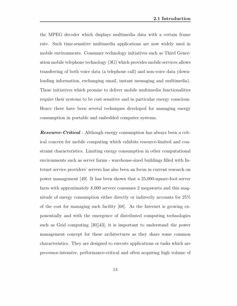
the MPEG decoder which displays multimedia data with a certain frame
rate. Such time-sensitive multimedia applications are now widely used in
mobile environments. Consumer technology initiatives such as Third Gener-
ation mobile telephone technology (3G) which provides mobile services allows
transferring of both voice data (a telephone call) and non-voice data (down-
loading information, exchanging email, instant messaging and multimedia).
These initiatives which promise to deliver mobile multimedia functionalities
require their systems to be cost sensitive and in particular energy conscious.
Hence there have been several techniques developed for managing energy
consumption in portable and embedded computer systems.
Resource-Critical - Although energy consumption has always been a crit-
ical concern for mobile computing which exhibits resource-limited and con-
straint characteristics. Limiting energy consumption in other computational
environments such as server farms - warehouse-sized buildings filled with In-
ternet service providers’ servers has also been an focus in current research on
power management [49]. It has been shown that a 25,000-square-foot server
farm with approximately 8,000 servers consumes 2 megawatts and this mag-
nitude of energy consumption either directly or indirectly accounts for 25%
of the cost for managing such facility [68]. As the Internet is growing ex-
ponentially and with the emergence of distributed computing technologies
such as Grid computing [30][43], it is important to understand the power
management concept for these architectures as they share some common
characteristics. They are designed to execute applications or tasks which are
processor-intensive, performance-critical and often acquiring high volume of
14

2.2 Power Management Strategies
data transfer. These characteristics are responsible for the majority of energy
consumption and the rapid development in processors and memory perfor-
mance also leads to a rapid growth in energy consumption. An example is
the growth in the chip die’s power density which has reached three times that
of a hot plate despite of the improvement of the circuit design [49]. Hence it
is important to manage energy consumption in these resource-critical com-
putational environments.
2.2 Power Management Strategies
There are many ways to analyse, optimise and manage energy consumption
in any computational environments. This chapter reviews these techniques
by spliting them into three distinct categories:
• Traditional/General Purposes
• Micro/Hardware Level
• Macro/Software Level
2.2.1 Traditional/General Purpose
Power management for computer systems has traditionally focused on regu-
lating the energy consumption in static modes such as sleep and suspend [10].
These are states or modes of a computational system which requires human
15

2.2 Power Management Strategies
interaction to activate/deactivate. Many power management mechanisms
are built into desktop and laptop computers through BIOS support with a
scheme called the Advanced Power Management (APM) [38] or via the oper-
ating system with an interface called the Advanced Configuration and Power
Interface (ACPI) [3].
APM is a BIOS-based system of power management for devices and
CPUs. It provides functionalities such as reducing clock speed when there
is no work to be done, which can significantly reduce the amount of energy
consumed. This means that the CPU will be slowed when idle. This is
an advantage to mobile computers as they are generally used for interactive
software and so it is expected to share a large amount of CPU idle time.
APM is configured to provide devices in these power states: ready, stand-by,
suspended, hibernation and off.
ACPI is an operating system oriented power management specification.
It is part of an initiative to implement the Operating System Power Man-
agement (OSPM) [3] which is an enhancement to allow operating systems
to interface and support ACPI-defined features such as device power man-
agement, processor power management, battery management and thermal
management. ACPI/OSPM enables computer systems to exercise moth-
erboard configuration and power management functions, using appropriate
cost/function trade offs. ACPI/OSPM replaces APM, MPS, and PnP BIOS
Specifications [2] and allows complex power management policies to be imple-
mented at an operating system level with relatively inexpensive hardware.
16

2.2 Power Management Strategies
Unlike APM which is solely BIOS-based, ACPI gathers information from
users applications and the underlying hardware together into the operating
system to enable better power management. ACPI also categorises different
platforms for power management and they are described as follows:
Desktop PC - these can be separated into Home PC and Ordinary “Green
PC”. Green PC is mostly used for productivity computation and therefore
requires minimal power management functions and the machine will stay in
working state all the time, whereas Home PC are computers designed for gen-
eral home purpose such as multimedia entertainment or answering a phone
call and they require more elaborate ACPI power management functionali-
ties.
Multiprocessor/Server PCs - these are specially designed server ma-
chines, used to support large-scale networking, database and communications
and require the largest ACPI hardware configuration. ACPI allows these ma-
chines to be put into Day Mode and Night Mode. During day mode, these
machines are put into working state. ACPI configures unused devices into
low-power states whenever possible.
Mobile PC - these machines require aggressive power management such
as thermal management and the embedded controller interface within the
ACPI. Thermal management is a function in which ACPI allows OSPM to
be proactive in its system cooling policies. Cooling decisions are made based
on the application load on the CPU and the thermal heuristics of the system.
Thermal management provides three cooling policies to control the thermal
17

2.2 Power Management Strategies
states of the hardware. It allows OSPM to actively turn on a fan. Turning
on a fan might induce heat dissipation but it cools down the processing units
without limiting system performance. It also allows OSPM to reduce the
energy consumption of devices such as throttling the processor clock. OSPM
can also shut down computational units at critical temperatures. Some mo-
bile devices which run operating systems such as Microsoft Windows CE
can also be configured to use its tailored power manager [59] which allows
users/OEMs to define any number of OS power states and does not require
them to be linearly ordered.
In observing the behaviour of a typical personal computer, both clock
speed and a spinning storage disk consume most of the consumable energy.
Therefore proper disk management also constitutes a major part in power
management [24]. ACPI provides a unified device power management func-
tion that allows OSPM to lower the energy consumption of storage disks by
putting them into sleeping states after a certain period of time. However
disk management policies in ACPI do not fulfil the requirement for current
demand for energy conscious computational components in both resource-
limited and resource-critical environments. Meanwhile some disk manage-
ment policies have been implemented to support such demand which will be
discussed in later sections.
Traditional power managements are considered to be static, application-
independent and not hardware oriented. These techniques have proved to
be insufficient when dealing with more specific computation environments
18

2.2 Power Management Strategies
such as distributed or pervasive environments. For example some scientific
applications might require frequent disk access and if these applications or
underlying systems are not optimised, the latencies and overheads created by
the disk entering and exiting its idle state might consume more energy than
just leaving it at working states. Therefore the following sections consider
other power managements which are more specific and dynamic.
2.2.2 Micro/Hardware Level
To devise a more elegant strategy for power management, many researchers
have dedicated their works to the reduction in energy consumption by in-
vestigating energy usage related to CPU architecture, system designs and
memory utilisation. These low-level analyses allow code optimisation and
adaptive power management policies. While the implementations of differ-
ent code optimisation techniques are discussed in section 2.2.3 under the
heading macro/application level analysis, an understanding of how an appli-
cation operates at a hardware level will enhance the ability to transform the
application source to optimise energy consumption. Three areas which are
described here are RT level and gate level analysis, instruction level analysis
and memory level analysis.
19

2.2 Power Management Strategies
2.2.2.1 RT and Gate Level Analysis
RT and gate level power analysis [74][75][50] are the lowest level of hardware
analyses in the field of power analysis. At this level, researches are more
concerned with RT and circuit level designs.
[75] presents a power analysis technique at an RT-level and an analytical
model to estimate the energy consumption in datapath and controller for a
given RT level design. This model can be used as the basis of a behavioural
level estimation tool. In the authors’ work they used the notion of FSMD
(Finite State Machine with a Datapath) as the architectural model for digital
hardware and this includes the SAT (State Action Table) which is defined
logically as follows:
~V = (v1, v2, ..., vn)
~V# ~W = (v1, v2, ..., vn, w1, w2, ..., wn)
~t = ~S#~C# ~NS# ~FU# ~Reg# ~Bus# ~Drv
SAT = {~ti}
ST = [~t1, ~t2, ..., ~tn]
SAT is used to describe the behaviour of a RT level design as distinctive
state tuples ~t which is a concatenation of some activity vectors ~V. Inside
each ~V is a collection of boolean states vi ∈ {0, 1}. A set of activity vectors
20

2.2 Power Management Strategies
can then be used to characterise a particular state of the hardware,namely
the current state vector ~S, the status vector ~C, the next state vector ~NS, the
function unit vector ~FU, the the register vector ~Reg, the bus vector ~Bus
and the the bus driver vector ~Drv. The estimation process of the RT level
energy consumption is carried out through the use of the state trace ST,
which is also defined logically and shown above, and it represents the actual
execution scenario of the hardware.
Unlike the previous analysis technique [75] which uses FSM, in [74] the
author proposed a cycle-accurate macro-model for RT level power analy-
sis. The proposed macro-model is based on capacitance models for circuit
modules and activity profiles for data or control signals. In this technique
simulations of modules under their respective input sequences are replaced
by power macro-model equation evaluation and this is said to have faster per-
formance. The proposed macro-model predicts not only the cycle-by-cycle
energy consumption of a module, but also the moving average of energy
consumption and the energy profile of the module over time.
The authors proposed an exact power function and approximation steps
to generate the power macro-model, the workflow of generating macro-model
is described in figure 2.1. The macro-model generation procedure consists of
four major steps: variable selection, training set design, variable reduction,
and least squares fit. Other than the macro model, the authors also proposed
first-order temporal correlations and spatial correlations of up to order three
and these are considered for improving the estimation accuracy. A variable
21

2.2 Power Management Strategies
Exact Power Function Large Population
Order Reduction
Variable Grouping
Stratified Random
Sampling
Powermill Simulation
Sensitivity Analysis/
Variable Reduction
Least-Square Fit
Initial Macro-model
Equation
Training Set
{(vector pair, power),...}
Accurate
Model?
Done
Figure 2.1: The workflow of generating a cycle-accurate macro-model [74].
reduction algorithm is designed to eliminate the insignificant variables using
a statistical sensitivity test. Population stratification is employed to increase
the model fidelity.
In [50] the author explored a selection of techniques for energy estima-
tion in VLSI circuits. These techniques are aimed at a gate-level and are
motivated by the fact that power dissipations of chip components such as
gates and cells happen during logic transitions and these dissipations are
highly dependent on the switching activity inside these circuits. The power
22

2.2 Power Management Strategies
dissipation in this work is viewed to be “input pattern-dependent”. Since
it is practically impossible to estimate power by simulating the circuit for
all possible inputs, the author introduced several probabilistic measures that
have been used to estimate energy consumption.
By introducing probabilities to solve the pattern-dependence problem,
conceptually one could avoid simulating the circuit for a large number of
patterns and then averaging the results, instead one can simply compute
from a large input pattern set the fraction of cycles in which an input signal
makes a transition and use that information to estimate how often internal
nodes transition and, consequently, the power drawn by the circuit. This
technique only requires a single run of a probabilistic analysis tool which
replaces a large number of circuit simulation runs, providing some loss of
accuracy being tolerated.
The computation of the fraction of cycles in which an input signal makes
a transition is known as a probabilistic measure and the author then intro-
duced several probabilistic techniques such as signal probability, CREST (a
probabilistic simulation using probability waveform), DENSIM (transition
density which is the average number of transitions per second at a node in
the circuit), a simple BDD (boolean decision diagram) technique and a corre-
lation coefficients technique whereby the probabilistic simulation is proposed
using correlation coefficients between steady state signal values are used as
approximations to the correlation coefficients between the intermediate signal
values. This allows spatial correlation to be handled approximately.
23

2.2 Power Management Strategies
2.2.2.2 Instruction Analysis and Inter-Instruction effects
Instruction analysis allows energy consumption to be analysed from the point
of view of instructions which provides an accurate way of measuring the en-
ergy consumption of an application via a model of machine-based instruc-
tions [70]. This technique has been applied to three commercial architec-
turally different processors [71]. Although it is arguable that instruction
analysis is part of application level analysis, it nevertheless helps developers
to gather information at a reasonably low “ architectural” level and at the
same time helps implementing any application changes based on them.
In this technique, current being drawn by the CPU during the execution
of a program is physically measured by a standard off-the-shelf, dual-slope in-
tegrating digital ammeter, a typical program, which is used in this technique,
contains several instances of the targeted instruction (instruction sequence)
in a loop. During the program’s execution, it produces a periodic current
waveform which yields a steady reading on an ammeter. Using this method-
ology, an instruction-level energy model is developed by having individual
instructions assigned with a fixed energy cost called the base energy cost.
This base cost is determined by constructing a loop with several instances of
the same instruction. The current being drawn whilst executing the loop is
then measured through a standard off the shelf, dual-slope integrating digi-
tal ammeter. The author argued that regardless of pipelining when multiple
clock cycles instructions induce stalls in some pipeline stages, the method of
deriving base energy cost per instruction remains unchanged [70]. Table 2.1
24

2.2 Power Management Strategies
Instruction Base Cost (mA) CyclesMOV DX,BX 302.4 1ADD DX,BX 313.6 1ADD DX,[BX] 400.1 2SAL BX,1 300.8 3SAL BX,CL 306.5 3
Table 2.1: Subset of base cost table for a 40MHz Intel 486DX2-S Series CPU
shows a subset of the base cost table for a 40MHz Intel 486DX2-S Series
CPU, taken from [70].
Table 2.1 shows a sequence of instructions assembled from a segment of a
running program, the numbers in column 2 are the base cost in mA per clock
cycle. The overall base energy cost of an instruction is the product of the
numbers in column 2 and 3, the supply voltage and the clock period. There-
fore it is possible to calculate the average current of this section using these
base costs. However, this average current is only an estimate, to enable the
derivation of an accurate value, variations on base costs due to the different
data and address values being used during runtime have to be considered.
An examples will be an instructions using memory operands since accessing
memory incurs variation in base costs. Also mis-alignment can induce cycle
penalties and thus energy penalties [37].
When sequences of different instructions are measured, inter-instruction
effects affect the total cost of energy consumption, however this type of effect
cannot be shown in base costs calculation. Through detail analysis [70], it is
possible to observe inter-instruction effects which are caused by the switching
activity in a circuit and they are mostly functions of the present instruction
25

2.2 Power Management Strategies
input and the previous state of the circuit. Other inter-instruction effects
include resource constraints causing stalling which also increases the number
of cycles for instruction execution, an example of such resource constraints is
a prefetch buffer stall. The effects of memory related overhead are discussed
in the next section.
2.2.2.3 Memory Power Analysis
Apart from a processor’s energy consumption, data transfers to and from
any kind of memory also constitute a major part in the energy consumption
of an application. Some research has been carried out to cater for this type
of analysis [6][61][54]. There are six possible types of memory power models
according to [61].
1. DIMM-level estimates - a simple multiplication of number of Dual
In-line Memory Modules (DIMM) in a machine and the power per
DIMM as quoted by the vendor. Simple but prone to inaccuracy.
2. Spread Sheet Model - this method calculates energy consumption
based on current, voltage, using some simple models such as the spread-
sheet provided by Micron [40].
3. Trace-based Energy-per-operation calculation - this method is
carried out by keeping track of a trace of memory reference made by
each running workload.
26

2.2 Power Management Strategies
4. Trace-based Time and Utilisation calculation - such power cal-
culation is carried out by using memory traces coupled by timing in-
formation. Based on this information and memory service-time para-
meters, it is possible to produce average power values at one or more
intervals of time. With the average power over these intervals, energy
can be calculated [61].
5. Trace-driven simulation - this type of simulation tracks the activ-
ity of the various components of the memory and simulates current
drawn by using some memory power analyses. Based on the current
provided by the simulation and supplied voltage, power dissipation can
be calculated.
6. Execution-driven simulation - similar to trace-based simulation,
however, the simulation framework and the source of the memory re-
quest is different. This type of simulation is the most complex to im-
plement for energy calculation.
In general memory systems have two sources of energy loss. First, the
frequency of memory access causes dynamic losses. Second, leakage current
contributes to energy loss [49]. In general there are two areas of memory
analysis that can be described:
1. Memory Organisation - organising memory so that an access acti-
vates only parts of it can help limiting dynamic memory energy loss.
By placing a small filter cache in front of the L1 cache, even if this fil-
27

2.2 Power Management Strategies
ter cache only has 50% hit rate, the energy saved is half the difference
between activating the main cache and the filter cache, and this is very
significant [49]. Furthermore, the current solution for current leakage
is to shut down the memory which is impractical as memory loses state
and shutting down the memory frequently can incur both energy and
performance losses. Other architectural improvements have been to re-
organise the cache memory which is carried out to separate L1 cache
with data and instructions [11]. This technique allowed biased pro-
grams such as one which is data-intensive to run without jeopardising
the performance of the program.
2. Memory Accesses - accessing memory via a medium such as a bus
is also a major factor of energy loss [49]. One way to reduce this loss is
to compress information in the address line reducing successive address
values. This type of code compression results in significant instruction-
memory savings, especially if the program stored in the system is only
decompressed on the fly during a cache miss.
A cache miss itself constitutes some degree of energy loss as each cache
miss leads to extra cycles being consumed. In [20] the author introduced
a conflict detection table, which stores the instruction and data addresses
of load/store instructions, as a way to reduce cache misses. By using this
table it is possible to determine if a cache miss is caused by a conflict with
another instruction and appropriate action can be taken. One could also
minimise cache misses by reducing memory accesses through imposing better
utilisation of registers during compilation. In [71] an experiment was carried
28

2.2 Power Management Strategies
out whereby optimisations were performed by hand on assembly code to
facilitate a more aggressive use of register allocation. The energy cost in
that particular experiment shows a 40% reduction in the CPU and memory
energy consumption for the optimised code, another way to enhance more
aggressive use of registers is to have larger register file, however accessing
larger register file will usually induce extra energy cost.
2.2.2.4 Disk Power Management
In terms of hardware level power analysis and in particular memory usage,
many researches have focused on power analysis and management at disk
level [24][32].
In [24], the authors identified the significant difference in the energy con-
sumption of idle and spinning disks. This is especially the case in a mobile
computational environment. The author hence proposed both online and
offline algorithms for choreographing the spinning up and down of a disk.
They are described as follows:
• OPTIMAL OPTIMAL - The proposed offline algorithm is based on the rel-
ative costs of spinning or starting the disk up. It uses future knowledge
to spin down the disk and to spin it up again prior the next access.
• OPTIMAL DEMAND - This is an alternative offline algorithm proposed by
the authors which assumes future knowledge of access times when de-
ciding whether to spin down the disk but it delays the first request
29

2.2 Power Management Strategies
upon spin-up.
• THRESHOLD DEMAND - This is not originated from the authors’ proposal
but it follows the taxomonies describing the choreography of the spin-
ning up and down if a disk. This is an online algorithm which spins
down the disk after a fixed period of inactivity and spins it up upon
the next access. This approach is most commonly used in present disk
management.
• THRESHOLD OPTIMAL - This algorithm spins down the disk after a fixed
period (similar to THRESHOLD DEMAND hence the word THRESHOLD) and
spins it up just before the next access. The authors have pointed out
the inefficiency of this algorithm as the possibility of an immediate disk
access following a disk spin down might mean not having enough time
to spin up the disk for this access and hence causing access delay.
• PREDICTIVE DEMAND - This algorithm uses a heuristic based on the pre-
vious access to predict the following disk spin down whereas spin-up is
performed upon the next access which is similar to THRESHOLD DEMAND’s
spin up policy.
• PREDICTIVE PREDICTIVE This algorithm uses a heuristic based on the
previous access to predict the following disk spin down as proposed in
PREDICTIVE DEMAND and also uses heuristics to predict the next spin
up.
Conversely, in [32][31], the authors looked at disk energy consumption
of servers in high performance settings. As the authors explained that the
30

2.2 Power Management Strategies
increasing concern of servers’ energy consumption is based on the growth of
business enterprises such as those providing data-centric services which use
components such as file servers and Web portals. They then further explained
a new approach which uses a dynamic rotation per minute (DRPM) approach
to control the speed in server disk array as they believed the majority of
energy expenditure comes from input/output subsystems and the DPRM
technique can provide significant savings in I/O system energy consumption
without reducing performance. The proposed technique dynamically mod-
ulates the hard-disk rotation speed so that the disk can service request at
different RPMs. Whilst the traditional power management (TPM) which
targets on single-disk applicational usage such as laptops and desktops, it is
difficult to apply TPM to servers. A characteristic of servers which makes
TPM unsuitable is when server workloads create continuous request stream
and it must be serviced. This is very different to the relatively intermittent
activities which characterises the interactiveness of desktops and laptops.
The advantage of this technique is that dynamically modulating the disk’s
RPM can reduce the energy consumption the spindle motor causes. Using
DRPM exploits much shorter idle periods than TPM can handle and also
permits servicing requests at a lower speed, allowing greater flexibilities in
choosing operating points for a desired performance or energy level. DRPM
can also help strike the balance between performance and power tradeoffs
while recognising that disk requests in server workloads can present relatively
shorter idle times.
31

2.2 Power Management Strategies
2.2.3 Macro/Application Level Analysis
Dynamic power management refers to power management schemes imple-
mented while programs are running. Recent advance in process design tech-
niques has led to the development of systems that support very dynamic
power management strategies based on voltage and frequency scaling [10].
While power management at runtime can reduce energy loss at the hardware
level, energy-efficiency of the overall system depends heavily on software de-
sign [9]. The following describes recent researches which focus on source code
transformations and optimisations [18][67][56], and energy-conscious compi-
lations [63].
2.2.3.1 Source Code optimisation/transformation
These techniques are carried out at the source code level before compilation
takes place. In this section several techniques are studied.
Optimisation using Symbolic Algebra - In [56] the author proposed
a new methodology based on symbolic manipulation of polynomials, and a
energy profiling technique which reduces manual interventions. A set of tech-
niques has been documented in [58] for algorithmic-level hardware synthesis
and these are combined with energy profiling, floating-point to fixed-point
data conversion, and polynomial approximation to achieve optimisation. The
use of the energy profiler allows energy hot spots of a particular section of
code to be identified, these sections are then optimised by using complex
32

2.2 Power Management Strategies
algorithmic functions. Note it is necessary for source code to be converted
into polynomial representation when applying symbolic algebra techniques.
Although this work has been proposed for embedded software, the techniques
used can also be applied in a wider spectrum. Currently this work has been
applied to the implementation of a MPEG Layer III (mp3) audio decoder [56].
Optimisation based on profiling - this type of source code optimisation
is carried out by using some profiling tools. This type of optimisations is gen-
erally applied at three levels of abstraction, they are algorithmic, data and
instruction-level [67]. The profiler utilises a cyclic accurate energy consump-
tion simulator [66] and relates the energy consumption and performance of
the underlying hardware to the given source code. This approach of using
layer abstraction in optimisation allows developers to focus first on a very
abstract view of the problem, and then move down in the abstraction and
perform optimisation at a narrower scope. It also permits concurrent opti-
misation at different layer. Similar to [56], this type of optimisation has been
applied to the implementation of a mp3 audio decoder [67].
Software Cost Analysis - while developers can potentially implement a
selection of algorithms that are energy conscious [67], it is difficult to auto-
mate the transition process and in many cases its effect highly depends on
the developer’s preferences. Similarly, although instruction-level optimisa-
tion can be automated, it is often strongly tied to a given target architecture.
In contrast, source code transformation, which is carried out by restructur-
ing source code, can be automated [7] and this type of optimisations is often
33

2.2 Power Management Strategies
independent of any underlying architecture. However, source code restruc-
turing can be problematic during the estimation of the energy saving in a
given transformation. One solution to this is to compile the restructured code
and execute it on a target hardware to measure its energy savings. Never-
theless, as this method is proved to be inefficient, in [18] a more abstract and
computationally-efficient energy estimation model is used, the author applied
this technique into two well-known transformation methods - loop unrolling
where it aims at reducing the number of processor cycles by eliminating loop
overheads, and loop blocking where it breaks large arrays into several pieces
and reuses each one without self interference.
2.2.3.2 Energy-conscious Compilation
In [63] the author proposed two compiler-directed energy optimisation strate-
gies based on voltage scaling. They are static and dynamic voltage scaling
respectively. This work aims at reducing energy consumption of a given
code without increasing its execution time. In static voltage scaling, a single
supply voltage level is determined by the compiler for the entire program.
While static voltage scaling is not as effective as dynamic voltage scaling, this
strategy converts the performance slack created by compiler optimisations to
energy benefit. Conversely, dynamic voltage scaling allows different voltage
supply levels to be set for different section of a given program code. This
compilation technique is based on integer linear programming and so it also
cater for the requirement of both energy and performance constraints.
34

2.3 Summary
The idea of voltage scaling came about when studying the energy con-
sumption of CMOS circuits. Their energy consumption is proportional to
KCV 2, where K is the switching rate, C is the capacitance and V is the
supply voltage [17], this quadratic relationship between the supply voltage
and energy consumption inspires the need to reduce the supply voltage. Much
research has been carried to take advantage of this relationship to reduce en-
ergy consumption and many techniques such as transistor sizing, threshold
voltage reduction have been developed [55][45]. While these techniques can
reduce energy consumption, by reducing voltage supply, execution time could
be increased [63].
2.3 Summary
This chapter documented a selection of the current research in the area of
power management, power-awareness in computational environments and
source code cost analyses. Techniques for power management and cost analy-
ses usually fall under one of three categories (Traditional and General Pur-
poses, Micro and Hardware Level, Macro and Software Level) and this chap-
ter described a number of tools that are associated with each of these cate-
gories. Of particular interest is the movement from low-level hardware power
management such as reducing cache misses [20] to high-level source code
transformation [56][18][67].
It is important to notice power-aware computing such as energy conscious-
35

2.3 Summary
ness is no longer restricted to areas of mobile computing or energy-limited
computational environments but is gradually moving towards the areas of
resource-critical computational environments such as parallel and distributed
computational environments, and the Grid [30][43] where energy consump-
tion has become a major factor to running cost [68]. Therefore to ensure a
low computational running cost, it is essential to develop new approaches to
predict an application’s energy consumption at a source code level and to
include this as a metric when building performance models.
36

Chapter 3
Power Analysis and Prediction
Techniques
3.1 Introduction
Whilst current research has produced a bank of techniques on power analysis
which are either software or hardware focused, they share some common
shortcomings:
Current techniques’ insufficiencies - The review of current power analy-
sis methodologies in chapter 2 suggests some important areas, which are
concerned with the development of designing a well-formed power analysis
strategy, that still need to be addressed. In particular, the majority of analy-
sis techniques that are currently available either require the analysers to have
37

3.1 Introduction
specific knowledge such as the low-level machine code or require the use of
specialised equipment. This technical knowledge and specialised equipments
might not be available during power analysis and such dependencies will
only hinder the flexibility of the analysis methodology. Furthermore, current
methodologies such as instruction level analysis [71] over emphasise the mea-
surement of absolute energy consumption. In the case of [71] analysers must
acquire the absolute measurement of the current drawn for every machine
instruction and this can undermine the usefulness of the analysis technique
itself.
In modern performance and cost analysis, there are three types of evalu-
ation techniques: analytical modelling, simulation and measurement. These
techniques offer different levels of accuracy, in particular, analytical modelling
requires so many simplifications and assumptions that high level accuracy is
not essential [39]. Unfortunately since current power analysis techniques sep-
arate themselves from the general performance evaluation domain, they lack
the ability to abstract the technicality of both target machine architectures
and target applications. To develop a well-formed power analysis strategy
means that such strategy should possess the flexibility similar to the ones in
the performance domain, so that level of accuracy can be varied and mea-
surement values can be relative.
Performance incompatibility - The current power analysis methodologies
are simply not compatible with the current advance in performance evalua-
tion and optimisation. Techniques which have been reviewed either neglect
38

3.1 Introduction
performance efficiency or isolate energy consumption from other performance
metrics such as execution time or memory utilisation. It is believed that
electrical energy is a major cost when running some large scale applications
and the cost of dissipating tens or potentially hundreds of megawatts is pro-
hibitive. This means during an overall cost analysis on performance measure,
energy consumption should be taken into account and should eventually be
integrated into performance characterisation and evaluation.
No standard characterisation model - To compensate for the shortcom-
ings of current power analysis strategies, a standard model is needed for
power analysis and it should allow applications to be systematically or hier-
archically optimised for energy consumption. As applications in recent years
are moving toward execution environments which are heterogeneous, distrib-
uted and even ubiquitous [16], without a standard model that can categorise
and characterise the energy usage of application’s workload generically, cur-
rent power analysis techniques will prove to be too inefficient and impractical.
Also by using an analytical model, it allows measurements to be based on a
hierarchical framework of relativity.
Following on from the weaknesses mentioned above, the proposed method-
ologies are aimed at developers without expertise in technical areas such as
low-level machine code and without specialised equipment to carry out energy
measurements. During the preliminary stages of this research we propose an
application-level power analysis and prediction technique which adopts the
performance evaluation framework and techniques developed by the High
39

3.2 Application-level Power Analysis and Prediction
Performance Systems Group [35] at the University of Warwick. Furthermore
this chapter introduces a theoretical concept to construct a power classifica-
tion model based on benchmark workloads. This model allows a more rel-
ative energy consumption prediction of an application, although this model
has not yet been fully implemented, some insights in choosing the relevant
characterisation units have been established.
3.2 Application-level Power Analysis and Pre-
diction
This analysis methodology is inspired by the Performance Analysis and Char-
acterisation Environment (PACE), a state-of-the-art performance evaluation
framework developed by the High Performance Systems Group at the Uni-
versity of Warwick [53]. In particular the proposed technique adopts the C
Application Characterisation Tool (capp) and the theory of the PACE re-
source modelling technique [53] [29]. The detail of this framework is briefly
explained below.
3.2.1 The PACE Framework
The motivation to develop PACE is to provide quantitative data concern-
ing the performance of sophisticated applications running on high perfor-
mance systems [14]. The framework of PACE is a methodology based on
40

3.2 Application-level Power Analysis and Prediction
a layered approach that separates the software and hardware systems com-
ponents through the use of a parallelisation template. This is a modular
approach that leads to readily reusable models, which can be interchanged
for experimental analysis.
The core component of PACE is a performance specification language,
CHIP3S (Characterisation Instrumentation for Performance Prediction of
Parallel Systems) [52] [14]. This language is used to create performance
model containing a number of analytical models that describe the performance-
critical elements of the application’s computational and inter-resource per-
formance. CHIP3S, which has similar syntax to C, makes it simpler for
developers to describe their application’s performance and create analyti-
cal performance models, without the requirement of detailed knowledge of
performance evaluation.
CHIP3S employs a layered approach to performance characterisation,
with each layer characterising a specific element of a parallel application
as shown in figure 3.1. When developing a performance model, each script is
associated with a specific layer within the framework in order to characterise
a specific performance-critical element of the application. These scripts im-
plement a defined object interface for each layer, providing a framework to
enable the re-usability of performance objects.
CHIP3S characterises applications as a control flow of synchronous micro-
blocks of either computational/inter-platform communication. Each block is
defined within a parallel template by a step declaration that states either
41

3.2 Application-level Power Analysis and Prediction
Application
Hardware
Parallel Template
Subtask
{Predicted Response Time}
{Model Parameters}
Figure 3.1: A layered methodology for application characterisation
the source, destination and size of a specific communication type or a refer-
ence to a characterised section of computation (declared within the subtask
that is associated with this template). This control flow of blocks within
a template characterises the parallelisation strategy of the subtask, that is
how this computation is spread among the available resources. The complete
performance model is a control flow of these subtasks. Each subtask, and
in turn each synchronous micro-block, is evaluated as declared within this
control flow model.
While the CHIP3S language is the core component of PACE, the PACE
framework as a whole is a combination of this language and a number of
application and hardware tools. The PACE toolkit contains a characterisa-
tion tool called capp [29], which automates the more time-consuming areas
of performance model development, a number of hardware benchmarks to
42

3.2 Application-level Power Analysis and Prediction
obtain timings for a platform’s computational and communication perfor-
mance, an analytical methodology for cache performance prediction [33] and
an evaluation engine that analytically calculates predictive traces of PACE
performance models.
The following is a brief description of the four layers shown in figure 3.1.
with an example of a performance object, written in CHIP3S, that is associ-
ated within each layer given for clarification. Each object is taken from the
characterised performance model of a simple matrix multiplication algorithm,
the source code of which is shown in listing 3.4.
1 static int **a,**c,**b;
2 static void multiply() {
3 int i,j,k;
4 for (i=0; i < 7000; i++)
5 for (k=0; k < 7000; k++)
6 for (j=0; j < 7000; j++) c[i][j] += a[i][k]*b[k][j];
7 }
Listing 3.4: A C implementation of matrix multiplication algorithm multi-plying two 7000x7000 square matrices
3.2.1.1 Application Object
A performance model uses an application object to act as an entry-point
to the model’s evaluation. Each application object declares the model’s pa-
rameters, the platform that the model is to be evaluated upon, and the
control flow of subtasks within the model. An example application object
43

3.2 Application-level Power Analysis and Prediction
file multiply app.la, taken from the characterised matrix multiplication
algorithm’s performance model, is shown in listing 3.5.
1 application multiply_app {
2 include hardware;
3 include mmult;
4 link {
5 hardware: Nproc = 1;
6 }
7 option {
8 hrduse = "IntelPIV2800";
9 }
10 proc exec init { call multiply_stask; }
11 }
Listing 3.5: multiply app.la - The application object of the matrix multi-plication algorithm’s PACE performance characterisation
Note that because this application is being modelled to be executed on
a single processor, therefore in this example the Nproc variable within the
hardware object is set to 1 (line 5) to indicate a sequential evaluation on one
processor. The Nproc variable within the hardware object is a link decla-
ration and it specifies the number of processors. This type of declarations
allows variables, or references to computation, to be initialised within other
performance objects before their evaluation. This declaration mechanism
also enables the passing of parameters within a model in order to control the
evaluation.
Another variable hrduse is set to a string value, valid in the application
and subtask objects. It controls the hardware model selection and must be
44

3.2 Application-level Power Analysis and Prediction
defined somewhere within the performance model. This variable is part of
the option declarations, currently there are three options available within
the CHIP3S language [36]. In this example, the hrduse option (line 8) is set
to IntelPIV2800 in order to evaluate this model with the Intel Pentium IV
2.8GHz hardware characterisation.
1 subtask multiply_stask {
2 include async;
3 link { async: Tx = multiply(); }
4 proc cflow multiply {
5 compute <is clc, FCAL, SILL>;
6 loop (<is clc, LFOR>, 7000) {
7 compute <is clc, CMLL, SILL>;
8 loop (<is clc, LFOR>, 7000) {
9 compute <is clc, CMLL, SILL>;
10 loop (<is clc, LFOR>, 7000) {
11 compute <is clc, CMLL, 3*ARL2, MILG, AILG, TILG, INLL>;
12 }
13 compute <is clc, INLL>;
14 }
15 compute <is clc, INLL>;
16 }
17 }
18 }
Listing 3.6: multiply stask.la - The subtask object of the matrix multi-plication algorithm’s PACE performance characterisation
To provide an entry point for application object to the model’s entire
evaluation, the declaration proc exec is used. They are generally used for
defining control flow within performance characterisations. All application,
subtask and parallel template objects must have one proc exec declaration
called init that is evaluated at the start of the object’s evaluation, and can
45

3.2 Application-level Power Analysis and Prediction
be used either to initialise any variable declarations defined or evaluate other
performance objects. This example declares one init proc exec declaration
that evaluates the multiply stask subtask object (line 10).
3.2.1.2 Subtask Object
A subtask object characterises an element of sequential computation. Apart
from declarations common to the application object there is the proc cflow
declarations that characterise computational performance. Listing 3.6 shows
an example subtask object file multiply stask.la, taken from the charac-
terised matrix multiplication algorithm’s performance model.
Other than the include declaration which references the async parallel
template object, and is used to characterise a sequential parallelisation strat-
egy, and the generic hardware object, there is also the variable Tx within the
async parallel template object which is referenced to the evaluated execu-
tion time of the multiply proc cflow declaration. This declaration is the
CHIP3S characterisation of the original multiply method within the algo-
rithm’s source code. Currently control flow sequences of an application can be
obtained by using capp (The C Characterisation Tool). Each of the control
flow sequences contains a number of elementary operations. These elemen-
tary operations are modelled by characterisations and include events such as
floating point multiplies, memory accesses and MPI communications. Costs
of these operations are archived in the hardware model of the underlying plat-
form. Details of this model are discussed in section 3.2.2.1. capp is a tool
46

3.2 Application-level Power Analysis and Prediction
that automates the construction of proc cflow statements within subtasks
by characterising the performance of an application’s C source code. Au-
tomating these characterisations greatly reduces the time required for PACE
performance model development, as well as ensuring that no mistakes are
made within these declarations. For this reason, capp was used in this ex-
ample to characterise the matrix multiplication algorithm multiply methods.
proc cflow characterisations can contain any number of four statements
that capture the method’s performance:
• Compute: This calculates the execution time of a list of instructions
that is given to the statement as parameters. For example, line 13
computes the execution time of the clc instruction INLL. To calculate
this, the parallel template that is evaluating this cflow looks up the
value associated with the INLL instruction in the hardware object being
used for the current evaluation. This value is then added to the total
predicted execution time for the current cflow. A more complicated list
of machine instructions can also be passed to the compute statement,
such as that shown at line 11.
• Loop: The Loop statement is a CHIP3S characterisation of an iterative
statement (for, while and so on) that is present in the original appli-
cation. The loop count of this iterative statement is characterised by
the statement’s second parameter. This variable may be a constant de-
fined previously in the subtask (7000 in the case of the loop statement
in line 6,8 and 10), or an expression that relates to a number of model
parameters that have been passed from the model’s application object.
47

3.2 Application-level Power Analysis and Prediction
• Case: The case statement is a CHIP3S characterisation of a condi-
tional statement (if, switch and so on) that is present in the origi-
nal application. This statement can define a number of performance
characterisations which are evaluated according to their probability of
execution.
• Call: The call statement evaluates another proc cflow statement,
adding the predicted execution time of that statement to the total
predicted execution time for the current cflow.
There are currently three methods to specify loop counts and case prob-
abilities while using capp:
#pragma capp If 0.5
if(x < y) {
...
#pragma capp Loop y_size
for(y = 0; y < y_size; y++) {
...
Listing 3.7: An example showing how to utilise the pragma statement forloop counts and case probabilities definitions
• Enter values when prompted by line number.
• Embed values in the source file itself. This is done using pragma state-
ments. loop or case statements should have a pragma statement on
the line immediately preceding them. The syntax is as follows: pragma
48

3.2 Application-level Power Analysis and Prediction
capp TYPE STRING, listing 3.7 shows some examples of embedding val-
ues into source codes.
• Provide a separate file containing all values, indexed by line number
with the syntax LINE-NUMBER:TYPE:STRING with TYPE and STRING de-
fined as for pragma statements. For example: 42:Loop:y size. The
main problem with this method of specifying values is that if the source
file changes, any line numbers in the probability file will no longer be
correct. For this reason, using pragma statements is usually preferable.
3.2.1.3 Parallel Template Object
1 partmp async {
2 var compute: Tx;
3 option { nstage = 1, seval = 0; }
4 proc exec init {
5 step cpu {
6 confdev Tx;
7 }
8 }
9 }
Listing 3.8: async.la - The parallel template object of the matrix multipli-cation algorithm’s PACE performance characterisation.
A parallel template object consists of a control flow of a number of syn-
chronous micro-blocks that characterise the parallelisation strategy of its
associated subtask object. Each block can either contain a specific com-
munication paradigm (defined by the source and destination platforms and
49

3.2 Application-level Power Analysis and Prediction
the size of the communication) or a computation that is evaluated on all
the available resources (the performance of which is characterised by a proc
cflow declaration within the subtask). A single micro-block is characterised
within CHIP3S by a step declaration.
The matrix multiplication algorithm is sequential and so a simple parallel
template that characterises the execution of the algorithm’s subtask on all
the resources is used within the algorithm’s performance model. This parallel
template object file async.la is shown in listing 3.8.
3.2.1.4 Hardware Object
A hardware object characterises the computational and inter-resource com-
munication performance of the underlying platform. CHIP3S characterises
a method’s performance as a control flow of machine-code instructions, and
the hardware object contains benchmarked timings for each of these instruc-
tions. During evaluation, timings for these instructions are located within
the specified hardware object and used to calculate the model’s predicted
performance. It is important to accurately measure these timings if accu-
rate predictive evaluations are to be achieved. An excerpt of an example
hardware object, for the IntelPIV2800 hardware object defined within the
matrix multiplication algorithm’s characterisation, is shown in listing 3.9.
By using the objects such as those defined in listings 3.5, 3.6 and 3.8
which are stored as .la files, an executable application model can be created
50

3.2 Application-level Power Analysis and Prediction
for the underlying resource specified by the hardware object as shown in
listing 3.9 by compiling these object files using the chip3s tool. This tool
generates some intermediate C codes which are then compiled into object
files. These object files are linked together with the CHIP3S runtime into an
executable. The building process is represented by the Makefile which is
shown in listing 3.10.
1 config IntelPIV2800 {
2 hardware {
3 Tclk = 1 / 2800,
4 Desc = "Intel Pentium IV/2.8GHz, Linux 2.6",
5 Source = "ip-115-69-dhcp.dcs.warwick.ac.uk";
6 }
7
8 (* C Operation Benchmark Program $Revision: 1.1 $
9 Timer overhead 2.82759000 *)
10
11 clc {
12 SISL = 0.000644827,
13 SISG = 0.000638161,
14 SILL = 0.000643161,
15 SILG = 0.000649827,
16 SFSL = 0.000608161,
17 SFSG = 0.000634827,
18 SFDL = 0.00120649,
19 SFDG = 0.00125149,
20 SCHL = 0.000634827,
21 SCHG = 0.000634827,
22 TISL = 0.0125282,
Listing 3.9: An excerpt of the IntelPIV2800.hmcl hardware object thatcharacterises the performance of a Pentium IV 2.8GHz processor.
51

3.2 Application-level Power Analysis and Prediction
1 all: multiply
2
3 multiply: multiply_app.o multiply_stask.o async.o
4 chip3sld -o $@ $^
5
6 %.o: %.la
7 chip3s -o $@ $<
Listing 3.10: The Makefile for building layer objects into runtime exeutable.
3.2.2 Moving Toward Power Awareness
Section 3.2.1 described one of the most comprehensive performance modelling
framework in parallel and distributed computing and this thesis documents
a novel technique of power analysis that utilises some of this framework’s
foundations, namely the C Characterisation Tool (capp), the C Operation
Benchmark Program (bench) and Hardware Modelling and Configuration
Language (HMCL). The proposed application-level power analysis concept it-
self is not only a branch of study on energy consciousness and power aware
computing, but it can also be implemented to extend the described perfor-
mance modelling framework for a more unified cost analysis system. This
section supplies more detail descriptions of the PACE components mentioned
above, and also gives an overview of the approach to develop a tool suite for
the proposed power analysis methodology.
52

3.2 Application-level Power Analysis and Prediction
3.2.2.1 HMCL: Hardware Modelling and Configuration Language
1 #define BENCH_STORE(op_name, op, limit, ovrhd) \
2 do { \
3 long __i, __j; \
4 double told, tnew; \
5 assert (limit % BLOCK == 0); \
6 startstats(#op_name); \
7 for(__i = 0; __i < REPEAT; __i++) \
8 { \
9 double opertime; \
10 told = BTimer(); \
11 for(__j = 0; __j < limit / BLOCK; __j++) { \
12 MULBLK(op) \
13 } \
14 tnew = BTimer(); \
15 opertime = ((TimeSub(tnew, told) - mtimerov) \
16 / (double)limit); \
17 stats(opertime); \
18 } \
19 outputstats(ovrhd, &op_name ## time); \
20 } while(0)
21
22 void AILL(void)
23 {
24 long a, b, c;
25 b = 32000000;
26 c = 43000000;
27 BENCH_STORE(AILL, a=b+c, LIMIT3, SILLtime);
28 }
29
Listing 3.11: An excerpt of the C Operation Benchmark Program writtento create instantaneous measurement of C elementary operations, showingone of the benchmarking macro and the implementation of the clc AILL
benchmarking method
53

3.2 Application-level Power Analysis and Prediction
HMCL is the language syntax allowing the PACE framework to define
the performance of the underlying hardware [51]. In this thesis, the primary
programming language studied is the C programming language. Here the
C Operation Benchmark Program - bench is used to create instantaneous
measurement of C elementary operations, listing 3.11 shows an excerpt of
this program depicting a benchmarking macro and an implementation of the
clc AILL 1 benchmarking method. This benchmark program measures a
number of computation micro-benchmarks, each corresponds to one C lan-
guage operation (clc). Each clc cflow operation is represented by a four-
character code and each proc cflow of a substask object contains statements
of cflow procedures as shown in listing 3.6. Each procedure is associated
with a processor resource usage vector (PRUV) [53]. The PRUV can take var-
ious forms ranging from low level operation count (e.g. CPU cycles, memory
references) up to high level descriptions (e.g. number of floating point oper-
ations). By combining the PRUVs with the resource model of the hardware
it is possible to predict the execution time of each software component. A
resource usage vector is associated with each statement that represents the
control flow of the application and these statements can be compute, loop,
case and call which have been described during the discussion of subtask
object in section 3.2.1.2.
To include the present resource model with energy consumption met-
rics, a new power-benchmarked hardware object is developed. Listing 3.12
shows an excerpt of the newly developed power-benchmarked hardware ob-
1add operation between two variables type long
54
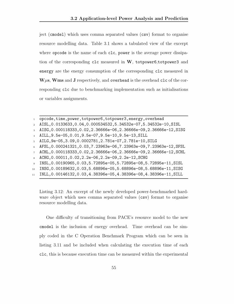
3.2 Application-level Power Analysis and Prediction
ject (cmodel) which uses comma separated values (csv) format to organise
resource modelling data. Table 3.1 shows a tabulated view of the excerpt
where opcode is the name of each clc, power is the average power dissipa-
tion of the corresponding clc measured in W, totpower6,totpower3 and
energy are the energy consumption of the corresponding clc measured in
Wµs, Wms and J respectively, and overhead is the overhead clc of the cor-
responding clc due to benchmarking implementation such as initialisations
or variables assignments.
1 opcode,time,power,totpower6,totpower3,energy,overhead
2 AISL,0.0133633,0.04,0.000534532,5.34532e-07,5.34532e-10,SISL
3 AISG,0.000118333,0.02,2.36666e-06,2.36666e-09,2.36666e-12,SISG
4 AILL,9.5e-05,0.01,9.5e-07,9.5e-10,9.5e-13,SILL
5 AILG,9e-05,3.09,0.0002781,2.781e-07,2.781e-10,SILG
6 AFSL,0.000241321,0.03,7.23963e-06,7.23963e-09,7.23963e-12,SFSL
7 ACHL,0.000118333,0.02,2.36666e-06,2.36666e-09,2.36666e-12,SCHL
8 ACHG,0.00011,0.02,2.2e-06,2.2e-09,2.2e-12,SCHG
9 INSL,0.00190965,0.03,5.72895e-05,5.72895e-08,5.72895e-11,SISL
10 INSG,0.00189632,0.03,5.68896e-05,5.68896e-08,5.68896e-11,SISG
11 INLL,0.00146132,0.03,4.38396e-05,4.38396e-08,4.38396e-11,SILL
Listing 3.12: An excerpt of the newly developed power-benchmarked hard-ware object which uses comma separated values (csv) format to organiseresource modelling data.
One difficulty of transitioning from PACE’s resource model to the new
cmodel is the inclusion of energy overhead. Time overhead can be sim-
ply coded in the C Operation Benchmark Program which can be seen in
listing 3.11 and be included when calculating the execution time of each
clc, this is because execution time can be measured within the experimental
55

3.2 Application-level Power Analysis and Prediction
opcode time power totpower6 totpower3 energy overheadAISL 0.0133633 0.04 0.000534532 5.34532e-07 5.34532e-10 SISLAISG 0.000118333 0.02 2.36666e-06 2.36666e-09 2.36666e-12 SISGAILL 9.5e-05 0.01 9.5e-07 9.5e-10 9.5e-13 SILLAILG 9e-05 3.09 0.0002781 2.781e-07 2.781e-10 SILGAFSL 0.000241321 0.03 7.23963e-06 7.23963e-09 7.23963e-12 SFSLACHL 0.000118333 0.02 2.36666e-06 2.36666e-09 2.36666e-12 SCHLACHG 0.00011 0.02 2.2e-06 2.2e-09 2.2e-12 SCHGINSL 0.00190965 0.03 5.72895e-05 5.72895e-08 5.72895e-11 SISLINSG 0.00189632 0.03 5.68896e-05 5.68896e-08 5.68896e-11 SISGINLL 0.00146132 0.03 4.38396e-05 4.38396e-08 4.38396e-11 SILL
Table 3.1: A tabular view of the cmodel excerpt shown in listing 3.12.
platform using internal C functions such as gettimeofday(). However, the
digital power measurement technique described in the thesis, which is also
used in the case study described in chapter 1, records instantaneous power
dissipation through an external digital power meter and its recordings are fed
into a data collection workstation, hence it is impossible to include overheads
dynamically into the benchmark measurements. Also equation 1.1 described
in chapter 1 is used to calculate the energy consumption of individual clcs,
and this means time overheads have to be included as part of the actual ex-
ecution time of the operation being benchmarked. This has been an issue in
both power analysis techniques described in this chapter. This is also one of
the factors which contribute to the inaccuracies of the measurements, these
factors are described in more detail in section 3.3.4.
56

3.2 Application-level Power Analysis and Prediction
3.2.2.2 Control Flow Procedures and Subtask Objects
1 Showing parse tree 0x95235b8:
2 10,0 TN_TRANS_LIST node 0x95235b8:
3 ..
4 1,0 Leaf node 0x9522758: Type static
5 ..
6 1,13 Leaf node 0x9522848: Identifier a
7 ...
8 1,17 Leaf node 0x9522910: Identifier c
9 Right Child 0x9522a28:
10 ...
11 Right Child 0x95229d8:
12 1,21 Leaf node 0x95229d8: Identifier b
13 ...
14 2,0 Leaf node 0x9522a50: Type static
15 ...
16 ...
17 3,6 Leaf node 0x9522bb8: Identifier i
18 Right Child 0x9522c30:
19 3,8 Leaf node 0x9522c30: Identifier j
20 Right Child 0x9522c80:
21 3,10 Leaf node 0x9522c80: Identifier k
22 Right Child 0x9522e38:
23 ...
24 ...
Listing 3.13: An excerpt of the parse tree generated by parsing the codeshown in listing 3.4.
As mentioned in the above sections, the main programming language un-
der investigation is C and the application-level characterisation technique
documented in this thesis adopts the C cpplication characterisation tool
capp for constructing control flow (cflow) definitions which defines the con-
57

3.2 Application-level Power Analysis and Prediction
trol flow of C language operations clc composition of the selected source
code. capp uses ctree which is a C Tree Parser package created by Shaun
Flisakowski [28] and it generates a parse tree. Listing 3.13 is an excerpt of
the parse tree generated by parsing the code shown in listing 3.4. capp uses
this parse tree to translate original source code into control flow procedure
proc cflow, an example of which is already shown in listing 3.6.
3.2.2.3 Trace Simulation and Prediction
Unlike PACE which produces the application execution model by using the
chip3s compiler, this thesis documents a divergence and proposes a more
dynamic set of tools known as PSim - Power Trace Simulation and Charac-
terisation Tools Suite. PSim is written in Java for its platform independence,
in particular it combines the strength of Java JFC/Swing to create an user in-
terface to give simulation capability for performance analysts and application
developers to visually examine both measured trace results and application
prediction analyses. Chapter 4 describes the details of PSim.
58

3.3 Power Analysis by Performance Benchmarking and Modelling
3.3 Power Analysis by Performance Bench-
marking and Modelling
Through binding the concept of characterisation and performance modelling [53],
an attempt has been made to express a power classification model to en-
hance the understanding of energy consumption at a high level abstraction.
It utilises benchmark workloads as nodes of the model and they represent
a certain construct or pattern of programming. Applications can then be
characterised or sectioned by these constructs or patterns, and they can be
matched by the corresponding nodes of the model and hence be able to obtain
a relative prediction of the application’s energy consumption.
The current construction of the classification model adopts both the ker-
nel and large-scale applications benchmarks from the Java Grande Bench-
mark Suite as elementary units of workloads, this selection of benchmark
workloads is chosen to cater for the diversity of applications running across
different hardware platforms. Whilst both kernel and large-scale applications
sections of the Java Grande Benchmark Suites [13], which has been trans-
lated into C programming language2, has been chosen as the preliminary
guideline for workload selections, to complete the classification model, the
benchmark workloads for low-level operations in the benchmark suites have
been manually translated into C. These workloads, each representing a node,
form a connected graph as the basic model which can act as a blueprint for
2The translation was designed to allow comparison of the sequential benchmarks withequivalent code written in C and Fortran [12].
59

3.3 Power Analysis by Performance Benchmarking and Modelling
constructing instants of classification models. Sections 3.3.1 and 3.3.2 dis-
sect the fundamentals of performance benchmarking and describes the Java
Grande Benchmark Suite. Section 3.3.3 describes the method used to mea-
sure the energy consumption of the C translated subset of the Benchmark
Suite and illustrates excerpts of the benchmark implementation, this sec-
tion also briefly explains the use of the classification model. Section 3.3.4
discusses the issues and areas of interest in the development of this power
analysis and modelling technique.
3.3.1 Performance Benchmarking
The idea of performance benchmarking is not new and there has been much
research work dedicated to performance analysis for serial applications run-
ning on a single hardware specification [22], multiple parallelised hardware
configurations [53] and heterogeneous distributed platform environments [72][53].
A benchmark is a workload used in the measurement of the process of per-
formance comparison for two or more systems. Many non-profit organisations
have developed numerous benchmarks of which each benchmark is executed
on a range of differently-performing platforms and execution environments,
in order to facilitate a performance-based comparison of these workloads on
different architectures. Benchmarks tend to be developed in suites, repre-
senting multiple workloads that characterise a set of similar computational
functionality. Benchmarking suites including a hierarchy of benchmarks that
attempt to identify the performance of varying aspects of a computing sys-
60

3.3 Power Analysis by Performance Benchmarking and Modelling
tem [4][34]. SPEC [21] have developed a wide range of benchmarks which
originally stresses the CPU, Floating Point Unit and to some extent the
memory subsystem, the organisation later developed benchmarks for graphi-
cal applications, workloads for high-performance applications, including Java
JVM workloads, client/server workloads, and even mail server benchmarks.
A large number of benchmarks are implemented to measure the performance
of a range of mathematical kernels, in order to facilitate comparison between
these kernel algorithms and their performances on a range of platforms.
These include, most notably, the LINPACK benchmarks for basic algebra
computations [23] and the NAS parallel benchmarks [8]. These benchmarks
have also been used to benchmark the performance of MPI-based mathe-
matical kernels, including Java Grande [13], which is the primary benchmark
suites to be explored in next section.
3.3.2 Java Grande Benchmark Suite
To bring power analysis into a high level abstraction and in tune with high
performance computing, a set of well known performance benchmarks has
been used. Over the past decade many performance benchmarks have been
implemented for large scale applications, in particular focus has been put
onto Java [13]. The Java Grande benchmark suite documented in [13] is a
popular resource within the high-performance community for evaluating the
performance of Java-based scientific applications. These benchmarks adopt
the hierarchical structure of the GENESIS Benchmark [4] which included
61

3.3 Power Analysis by Performance Benchmarking and Modelling
low-level operations, kernels and large scale applications sections. During
the development stage of the benchmark suite a subset of benchmarks has
been rewritten in C and FORTRAN to allow inter-language comparisons [12].
The C implementation of the benchmark suite has been adopted due to the
nature of C being able to interact with memory, devices and processors di-
rectly. Whereas the language comparison benchmark suite in C is divided
into kernels’ and large-scale applications’ sections, for the completeness of
constructing the power classification model, the section for elementary oper-
ations has also been translated from Java into C. Below is a brief outline of
the operations of individual benchmarks.
3.3.2.1 Elementary Operations
Elementary operation benchmarks are designed to test the performance of
the low-level operations such as addition using type float or looping and
indivisible operations such as I/O request or memory allocation, which will
ultimately determine the performance of real applications running under the
target platform. These benchmarks are designed to run for a fixed period of
time: the number of operations executed in that time is recorded, and the
performance reported as operations/second.
62

3.3 Power Analysis by Performance Benchmarking and Modelling
1 void ArithAddInt() {
2 size = INITSIZE;
3 i1=1; i2=-2; i3=3; i4=-4;
4 while (size < MAXSIZE){
5 for (i=0; i<size; i++){
6 i2+=i1;
7 i3+=i2;
8 ....
9 i3+=i2;
10 i4+=i3;
11 i1+=i4;
12 }
13 size *=2;
14 }
15 }
Listing 3.14: An excerpt of arith.c showing the integer add benchmarkmethod.
1. Arith measures the performance of arithmetic operations (add, multi-
ply and divide) on the primitive data types int, long, float and double.
Performance units are adds, multiplies or divides per second. List-
ing 3.14 is an excerpt of arith.c showing the integer add benchmark
method.
2. Assign measures the cost of assigning to different types of variable.
The variables may be scalars or array elements, and may be local vari-
ables, global variables or pointer variables. Performance units are as-
signments per second.
3. Memory This benchmark tests the performance of allocating and free-
ing physical memory. Memory sizes are allocated for arrays, matrices
63

3.3 Power Analysis by Performance Benchmarking and Modelling
(pointer to an array) of different data type and of different sizes. Per-
formance units are allocations per second.
4. Loop measures loop overheads, for a simple for loop, a reverse for loop
and a while loop. Performance units are iterations per second.
5. Method determines the cost of a method call. The methods can be
of no arguments, taking basic data type such as int as arguments or
taking complex data type such as a pointer or a pointer pointing to a
pointer. Performance units are calls per second.
6. Serial measures the performance of serialisation, both writing and
reading of a dataset to and from a file. The types of dataset tested
are arrays, matrices and binary data. Performance units are bytes per
second.
3.3.2.2 Kernels Section
A kernel is generalisation of some instruction mix. In some specialised ap-
plications, one can identify a set of common operations, for example matrix
inversion. Different processors can then be compared on the basis of their
performances on these kernel operations. Some of the commonly used ker-
nels are Sieve, Puzzle, Tree Searching, Ackerman’s Function, Matrix Inver-
sion, and Sorting. However, unlike instruction mixes, most kernels are not
based on actual measurements of systems. Rather, they became popular af-
ter being used by a number of researchers trying to compare their processors’
64

3.3 Power Analysis by Performance Benchmarking and Modelling
architecture. The following kernel benchmarks are chosen to be short codes
containing the type of computation likely to be found in Grande applications.
1. Fourier coefficient analysis computes the first N Fourier coefficient
of the function f(x) = (x + 1)x. This is computed on the interval 0,2.
Performance units are coefficients per second. This benchmark heavily
exercises transcendental and trigonometric functions.
2. LU factorisation solves an NxN linear system using LU factorisa-
tions followed by a triangular solve. This is a derivative of the well
known LINPACK benchmark [22]. Performance units are MFlops per
second. Memory and floating point intensive.
3. Heap Sort Algorithm sorts an array of N integers using a heap sort
algorithm. Performance unit is in units of items per second. Memory
and integer intensive.
4. Successive Over-relaxation performs 100 iterations of successive
over-relaxation on an NxN grid. The performance unit is in iterations
per second.
5. Fast Fourier Transform performs a one-dimensional forward trans-
form of N complex numbers. This kernel exercises complex arithmetic,
shuffling, non-constant memory references and trigonometric functions.
6. Sparse Matrix Multiplication performs matrix-vector multiplica-
tion using an unstructured sparse matrix stored in compressed-row for-
65

3.3 Power Analysis by Performance Benchmarking and Modelling
mat with a prescribed sparsity structure.
7. Matrix Inversion performs inversion on an NxN matrix using Gauss-
Jordan elimination with pivoting and hence solves N linear equations [60].
Listing 3.15 is an excerpt of matinvert.c showing matrix inversion
benchmark method using technique mentioned above.
3.3.2.3 Large Scale Applications
If computer systems are to be compared using a particular application, a
representative subset of functions for that application may be used. The
following benchmarks are intended to be representatives of some large scale
applications, suitably modified for inclusion in the benchmark suite by re-
moving any I/O and graphical components.
1 #define SWAP(a,b) {temp=(a);(a)=(b);(b)=temp;}
2
3 void Inverttest(float **a, int n, float **b, int m) {
4 int icol,irow,l,ll,i,j,k;
5 float big,dum,pivinv,temp;
6 for (j=1;j<=n;j++) ipiv[j]=0;
7 for (i=1;i<=n;i++) {
8 big=0.0;
9 for (j=1;j<=n;j++)
10 if (ipiv[j] != 1)
11 for (k=1;k<=n;k++) {
12 if (ipiv[k] == 0) {
13 if (fabs(a[j][k]) >= big) {
14 big=fabs(a[j][k]);
15 irow=j;
16 icol=k;
66

3.3 Power Analysis by Performance Benchmarking and Modelling
17 }
18 } else if (ipiv[k] > 1) nrerror("gaussj: Singular Matrix-1");
19 }
20 ...
21 }
22 for (l=n;l>=1;l--) {
23 if (indxr[l] != indxc[l])
24 for (k=1;k<=n;k++)
25 SWAP(a[k][indxr[l]],a[k][indxc[l]]);
26 }
27 }
Listing 3.15: An excerpt of matinvert.c showing matrix inversion bench-mark method using Gauss-Jordan Elimination with pivoting technique, notethe use of macro SWAP.
1. Computational Fluid Dynamics solves the time-dependent Euler
equations for flow in a channel with a “bump” on one of the walls.
A structured, irregular, Nx4N mesh is employed, and the solution
method is a finite volume scheme using a fourth order Runge-Kutta
method with both second and fourth order damping. The solution is
iterated for 200 time steps. Performance is reported in units of time
steps per second.
2. Molecular Dynamics simulation is an N -body code modelling
particles interacting under a Lennard-Jones potential in a cubic spa-
tial volume with periodic boundary conditions. Performance unit is in
interactions per second and the number of particles is give by N .
All the mentioned benchmarks within the suite have been modified to
tailor the need for performance benchmark power analysis described below.
67

3.3 Power Analysis by Performance Benchmarking and Modelling
3.3.3 Performance Benchmark Power Analysis
Figure 3.2: PSim’s Power Trace Visualisation bundle - graphical visualisa-tion of power trace data compiled by recording current drawn by a heapsortalgorithm
Performance Benchmark Power Analysis denotes the monitoring of energy
consumption while a particular workload is running on a targeted platform.
The monitoring is carried out externally by measuring and recording the
electric current passing through the main electric cable and the voltage across
it. The product of these yields the electrical power. This analysis adapts the
same approach and experimental platform as specified in the case study in
chapter 1, hence calculation can be carried out according to equation 1.1.
68

3.3 Power Analysis by Performance Benchmarking and Modelling
1 void NumHeapSort() {
2 int temp,i;
3 int top = array_rows - 1;
4 for (i = top/2; i > 0; --i)
5 NumSift(i,top);
6 for (i = top; i > 0; --i) {
7 NumSift(0,i);
8 temp = TestArray[0];
9 TestArray[0] = TestArray[i];
10 TestArray[i] = temp;
11 }
12 }
13
14 void NumSift(int min, int max) {
15 int k;
16 int temp;
17 while((min + min) <= max) {
18 k = min + min;
19 if (k < max)
20 if (TestArray[k] < TestArray[k+1]) ++k;
21 if (TestArray[min] < TestArray[k]) {
22 temp = TestArray[k];
23 TestArray[k] = TestArray[min];
24 TestArray[min] = temp;
25 min = k;
26 } else
27 min = max + 1;
28 }
29 }
Listing 3.16: An excerpt of heapsort.c showing a heap sort algorithm bench-mark method.
During Performance Benchmark Power Analysis, the chosen benchmark
workloads which have been rewritten and modified in C are executed on an
experimental platform. At every N iterations of the workloads’ execution,
apart from power dissipation is measured, a selection of resource information
69

3.3 Power Analysis by Performance Benchmarking and Modelling
is also recorded. Currently parts of the resource information include processor
cycle and memory utilisation.
Figure 3.2 shows screen shot of a graphical simulation in PSim displaying
a line representation of the power trace file compiled by recording current
drawn by a heap sort algorithm shown in listing 3.16. The vertical and
horizontal calibrations shown in the figure are the current drawn and the
execution time respectively. PSim is described in details in chapter 4. From
this graphical view it should be possible to depict repetitive patterns since
the algorithm is being executed for some N iterations.
1 static int a[];
2 static void bubblesort() {
3 int i,j,tmp;
4 for ( i=0; i<6999; i++) {
5 for (j=6999; j>i; j--) {
6 if ( a[j-1] > a[j] ) {
7 swap(&a[j-1],&a[j]);
8 }
9 }
10 }
11 }
12
13 static void swap(int *x,int *y) {
14 int tmp;
15 tmp = *x;
16 *x = *y;
17 *y = tmp;
18 }
Listing 3.17: A C implementation of bubble sort algorithm with 7000 integerarray.
70

3.3 Power Analysis by Performance Benchmarking and Modelling
3.3.3.1 Using the Classification Model
To demonstrate the concept of a power classification model, an implementa-
tion of the bubble sort algorithm shown in listing 3.17 is used as an example.
This bubble sort algorithm re-orders the integer values in pointer variable a.
By simply stepping through the source code it is possible to identify simple
workloads within its construct which represents the nodes of the basic model
mentioned above. For example line 4 and 5 can be matched to the node
loop which represents iteration construct, the implementation of the loop
workload benchmark is shown in listing 3.18. Line 7 which is a call to the
method swap can be matched to the node method as it represents the cost
of a method call, the implementation of the method workload benchmark is
shown in listing 3.19. Similarly, assuming the probability of executing line
7 is 0.5, we can also match line 15, 16 and 17 as global variable pointer as-
signment construct with the node assign, the implementation of the assign
workload benchmark is shown in listing 3.20.
1 void ArithLoop() {
2 size = INITSIZE;
3 while (size < MAXSIZE){
4 for (i=0;i<size;i++) {
5 }
6 size *=2;
7 }
8 }
Listing 3.18: An excerpt of arith.c showing the loop construct benchmarkmethod
71

3.3 Power Analysis by Performance Benchmarking and Modelling
1 static void ArithMethod() {
2 size = INITSIZE;
3 while (size < MAXSIZE){
4 for (i=0;i<size;i++) {
5 static_method();
6 static_method();
7 static_method();
8 static_method();
9 static_method();
10 ...
11 static_method();
12 static_method();
13 }
14 size *=2;
15 }
16 }
17
18 static void static_method(void) { }
Listing 3.19: An excerpt of arith.c showing the method workload bench-mark method
1 int *a1=1,*a2=2,*a3=3,*a4=4;
2 void ArithAssignGlobal() {
3 size = INITSIZE;
4 while(size < MAXSIZE){
5 for (i=0;i<size;i++) {
6 a1=a2;
7 a2=a3;
8 a3=a4;
9 a4=a1;
10 a1=a2;
11 a2=a3;
12 a3=a4;
13 ...
14 a3=a4;
15 a4=a1;
16 }
72

3.3 Power Analysis by Performance Benchmarking and Modelling
17 size *=2;
18 }
19 }
Listing 3.20: An excerpt of arith.c showing the assign workload bench-mark method
3.3.4 Observation
Although the example shown above is rather simple, it demonstrates the use
of the basic classification model, a more complex application might need to
utilise different levels or sections of the model i.e. kernel or grande. How-
ever observations show there are number of factors which might have major
significance to the development of this conceptual model. To enable further
development of this model, the following should be considered:
• Exhaustive Characterisation Units - The theoretical model has
not yet proven to be exhaustive at this preliminary stage. It is impor-
tant for the basic model to have an exhaustive collection of characteri-
sation/classification units and yet be extendable so that nodes or units
can be added or deleted as deemed necessary.
• Accuracy of the Analysis - Benchmarking results are considered to
be inaccurate for the basic model mentioned above. This has led to
the difficulty in creating concrete dependencies between workloads as
nodes in the model. The reasons for this inaccuracy are as follows:
73

3.4 Summary
1. Complexity of the platform and the black-box method of power
analysis create a noise floor for accurate results to be obtained,
the black-box method is discussed in section 4.3.
2. Frequency of measurement is too small in comparison to processor
cycles so that it is impossible to capture all the relevant power
dissipation during recording.
3. Each benchmark method has certain pre-conditions such as mem-
ory storage or variable initialisation and produces post-conditions.
These conditions affects the accuracy of the analysis.
• Concrete nodes connection - Although there is a hierarchical re-
lationship between the workloads by their complexity, it is not yet
possible to connect them as node into the classification model that can
be used to characterise applications relatively.
3.4 Summary
This chapter described two proposed techniques and concepts in power-
metric analysis and application predictions, they are namely application level
analysis by defining implementation language operations as blocks of control
flow definitions and power analysis by using a classification workload model.
This chapter also introduced a dynamic set of tools known as PSim - Power
Trace Simulation and Characterisation Tools Suite to employ the techniques
described in this chapter. PSim is implemented in Java for its platform inde-
74

3.4 Summary
pendence. The detail of PSim implementation is documented in chapter 4.
These power analysis techniques are both computational environment and
platform independent since the techniques mentioned abstract the underlying
platform into either the corresponding hardware object or an instantiation of
the basic model in performance benchmark power analysis, therefore in the-
ory, with the corresponding resource profile, applications can be analysed and
their energy consumption can be predicted for any types of computational
environment and platforms.
75

Chapter 4
PSim: A Tool for Trace
Visualisation and Application
Prediction
4.1 Introduction
Whilst formulating the energy consumption analysis and prediction tech-
niques, which have been described in chapter 3, a tools suite called PSim -
Power Trace Simulation and Characterisation Tools Suite is developed to em-
body these techniques. PSim is written in JavaTM (J2SE version 1.4.2) and
the source code contains about 10,000 lines. PSim is split into two bundles
76

4.1 Introduction
Entity/Description Implementation ClassesPower Trace Visualisation:To graphically visualise, playback Simulate, TimeChart,and analyse trace information Trace,TraceException,from application enery consumption printSummary, printTable, SimStepmeasurements.Characterisation and Prediction:To characterise and predict applications’ Simulate, Characterisation,energy consumption based on bSemaphore, SourceView,source code. TraceException
Table 4.1: A table showing an overview of the main functionalities of PSimand their corresponding implementation class.
and their main functionalities are listed in table 4.11. Power Trace Visuali-
sation is a bundle which provides detailed and dynamic graphical animation
as well as energy consumption analysis summaries based on recorded traces
from energy consumption analysis. Characterisation and Prediction is a bun-
dle which provides the capability to characterise and predict an application’s
energy consumption based on its source code. Section 4.2 describes the back-
ground and motivation of software visualisation, section 4.3 documents the
implementation and details of Power Trace Visualisation bundle (PTV) and
section 4.4 documents the implementation and details of Characterisation
and Prediction bundle (CP).
1The implementation package is uk.ac.warwick.dcs.hpsg.PSimulate and a simpli-fied UML class diagram of this Java package is shown in appendix C
77

4.2 Visualisation Motivation and Background
4.2 Visualisation Motivation and Background
Graphical visualisation is a standard technique for facilitating human com-
prehension of complex phenomena and large volumes of data [48]. This is
particularly crucial when investigating the behaviour of an application at a
source code level, coupling with their energy consumption activities. Thus
it seems natural to use visualisation techniques to gain insight into these
behaviours and activities so that application’s energy oriented performance
can be understood and improved.
Graphical visualisation of an applications’ performance activities is not
a new idea. In the past decade early graphical visualisation has already
addressed a wide variety of problems that range from algorithm animation
and visual programming to visualising software design issues of large-scale
systems. When visualising complex algorithms to assist comprehension and
analysis tasks associated with maintenance and re-engineering, it brings to-
gether research from software analysis, information visualisation, human-
computer interaction, and cognitive psychology. Research in software vi-
sualisation has flourished in the past decade and a large number of tools,
techniques, and methods were proposed to address various problems.
An analogy can be drawn between software visualisation and learning to
program. Programming is an activity that forces us to draw upon our abilities
to think analytically, logically, and verbally [65]. This requires using both
sides of our brain. The left hemisphere is responsible for analytical and logical
78

4.2 Visualisation Motivation and Background
thinking. The right hemisphere is responsible for more artistic and intuitive
thinking. It is also capable of processing in parallel to capture images as
a whole. In [65] the author gives four reasons why visual programming is
stimulated. They are as follows:
1. Pictures are a more powerful means of communication than words;
2. Pictures aid understanding and remembering;
3. Pictures can provide an incentive for learning to program;
4. Pictures are understood by people no matter what language they speak.
Similarly, understanding an application’s performance activities can be
augmented through the use of graphical visualisation. The power of a vi-
sualisation in programming language and representation is derived from its
semantic richness, simplicity, and level of abstraction which are also correct
when visualisng execution traces. The aim is to develop a representation
with fewer constructs, but at the same time with the ability to represent
a variety of elements with no ambiguity or loss of meaning. This section
gives an overview of some of the graphical visualisation tools for applica-
tions under two distinct types of computational environments, sequential
and parallel. Although the tools pertaining to these environments serve very
different purposes, nevertheless behind these visualisation tools lies a similar
motivation which is to allow greater understandings of both the applications’
constructs and their execution behaviour.
79

4.2 Visualisation Motivation and Background
4.2.1 Sequential Computational Environments
In the past, the goal of software visualisation in sequential environments is
to allow programs to run faster. There are three components to run-time
efficiency: algorithms, data structures and efficient coding [26]. To find the
inefficiencies in their code, programmers use a number of techniques to deter-
mine where the most CPU time is spent (“hotspot”) and then make changes
to reduce this time. Some of the techniques include “profiling” (enabling
code tuning) [26] (energy consious profiling is documented in section 2.2.3),
execution trace visualisation [62], and static analysis such as code browsing
with colour and height representation [27] [25]. In this section visualisation
tools Seesoft [27], Tarantula [62] and Source Viewer 3D [44], are described.
Seesoft - The Seesoft software visualisation system, developed by AT&T
Bell Laboratories employs the pixel metaphor and allows one to analyse up
to 50,000 lines of code simultaneously by mapping each line of code into
a thin row of pixels [27]. The display is similar to an extremely reduced
representation of code that has been typeset [26].
The system displays information through the use of version control, static
analyses such as verifying the locations where functions are called and dy-
namic analyses such as code profiling. It identifies “hot spots” in the code.
This type of visualisation techniques which is used for analysing profile data
also complements function summary techniques because it allows application
developers to study line oriented statistics. Seesoft employs a unique method-
ology that allows developers to discover usage patterns in the implementation
80

4.2 Visualisation Motivation and Background
code that would otherwise be infeasible using traditional methods.
Figure 4.1: Tarantula’s continuous display mode using both hue and bright-ness changes to encode more details of the test cases executions throughoutthe system [25].
Tarantula - SeeSoft-like representations are used by a number of existing
tools such as Tarantula [25] which implements fault localisation via visuali-
sation as the author believed that locating the faults which cause test case
failures is the most difficult and time-consuming component of the debugging
process. It employs a colour model to display each source code statement
that reflect its relative success rate of its execution by the test suite. An ex-
ample of it is shown in figure 4.1 which illustrates a screenshot of Tarantula
in continuous display mode. Although it is not obvious from the figure, this
81

4.2 Visualisation Motivation and Background
model renders all executed statements so that the hue of a line representing
individual statment is determined by the percentage of the number of failed
test executing statement s to the total number of failed tests in the test suite
T and the percentage of the number passed tests executing s to the number
of passed tests in T [25].
Source Viewer 3D - The Source Viewer 3D (sv3D) [46] is a framework
for software visualisation which augmented Seesoft’s pixel metaphor by in-
troducing a 3D metaphor to represent software system and containers, poly
cylinders, height, depth, color and position.This 3D metaphor extends the
original one by rendering the visualisation in a 3D space. sv3D supports
zooming and panning at variable speed which have been proven to be impor-
tant when the examined application or the visualisation space is large. sv3D
brings the following major enhancements over Seesoft-type representations:
• It creates 3D renderings of the raw data.
• Various artifacts of the software system and their attributes can be
mapped to the 3D metaphors, at different abstraction levels.
• It implements improved user interactions.
• It is independent of the analysis tool.
• It accepts a simple and flexible input in XML format. The output of
numerous analysis tools can be easily translated to sv3D input format.
• Its design and implementation are extensible.
82

4.2 Visualisation Motivation and Background
Figure 4.2: an element of visualisation in sv3D displaying a container withpoly cylinders (P denoting one poly cylinder), its position Px,Py, height z+,depth z
−, color and position [46].
Apart from fault localisation, visualisation of execution traces, source
code browsing, impact analysis, evolution and slicing, sv3D also uses height
instead of brightness (as in Tarantula) which will improve the visualisation
and make the user tasks easier.
4.2.2 Parallel Computational Environments
The behaviours of parallel applications are often extremely complex, and
hardware or software performance monitoring of such applications can gen-
83

4.2 Visualisation Motivation and Background
erate vast quantities of data. Thus, it seems natural to use graphical visual-
isation techniques to gain insight into the behaviour of parallel applications
so that their performance can be understood and improved.
Over the last ten years or so a number of powerful tools have emerged for
visualising parallel applications. These are essentially “discrete event mon-
itoring” tools, which are able to display time-line information of individual
parallel processes and show a graph of the active communication events dur-
ing the execution. This may be supplemented by user-defined events enabling
the programmer to identify the area of code being displayed.
The two tools set which are descibed are ParaGraph [48] and Parade [69].
ParaGraph is based on PICL (Portable Instrumented Communication Li-
brary), developed at Oak Ridge National Laboratory and available from
netlib2, and it is used as a graphical display tool for visualising the behav-
iour and performance of parallel applications that use MPI (Message-Passing
Interface). Parade is a comprehensive environment for developing visualisa-
tions and animations for parallel and distributed applications. It includes
components such as an animation toolkit for visualising applications from
many different languages and on many different architectures and an anima-
tion choreographer which provides flexible control of the temporal mapping
programs to the environment’s animations.
ParaGraph - ParaGraph is a graphical display system for visualising the
behaviour and performance of parallel programs on message-passing parallel
2Available at http://www.netlib.org/picl/
84

4.2 Visualisation Motivation and Background
Categories Display ComponentsUtilization Processor count, Gantt chart, Summary,
Concurrency profile, Utilization meter,Kiviat diagram
Communication Message Queues, Communication matrix,Animation, Hypercube, Communication meter,Communication traffic, Space-time diagram
Task Information Task Gantt, Task summary
Table 4.2: A table showing categories of display and their associated compo-nents of ParaGraph [48].
computers [48]. It takes trace data provided by PICL as input execution.
PICL is a subroutine library that implements a generic message-passing in-
terface on a variety of multiprocessors. Programs written using PICL rou-
tines instead of the native commands for interprocessor communication are
portable in the sense that they can be run on any machine on which the
library has been implemented. PICL also optionally produces an execution
trace during an actual run of a parallel program on a message-passing ma-
chine, and the resulting trace data can then be replayed pictorially with
ParaGraph to display a dynamic, graphical depiction of the behaviour of the
parallel program.
ParaGraph provides several distinct visual perspectives from which to
view processor utilisation, communication traffic, and other performance
data in an attempt to gain insights that might be missed by any single view.
Table 4.2 describes these display categories in ParaGraph.
Its basic structure is that of an event loop and a large switch that selects
actions based on the nature of each event. There are two separate event
85

4.2 Visualisation Motivation and Background
queues: a queue of X events produced by the user on events such as mouse
clicks, keypresses and window exposures and a queue of trace events produced
by the parallel program under study. ParaGraph alternates between these
two queues to provide both a dynamic depiction of the parallel program and
responsive interaction with the user
Parade - Parade supports the design and implementation of software visu-
alisations of parallel and distributed programs [69]. One of Parade’s compo-
nents is the visualisaton of a program execution, it utilises trace information,
and relies on software-level instructmentation which is used for performance
monitoring and can be performed at different levels such as operating system,
run-time system, system-supplied libraries etc. Common software visualisa-
tions for program monitoring using Parade are run post-mortem i.e. the
testing application produces a trace which is post-processed at a later time.
This method is carried out using the animation choreographer, figure 4.3
shows a user interface for the animation choreographer that presents the or-
dering and constraints between program execution events [69]. One major
breakthrough in program monitoring using Parade is the technique for per-
forming on-line visualisation which involves mechanisms to transmit program
event to the animation components “intelligently”. This technique relies on
filtering which can perserve the causal ordering of execution events and this
is achieved by applying simple ordering rules to the event transmissions.
86

4.3 Power Trace Visualisation
Figure 4.3: User interface for the animation choreographer that presents theordering and constraints between program execution events [69].
4.3 Power Trace Visualisation
PSim adopts a “playback” mechanism which resembles a similarity to Para-
Graph [48] mentioned in section 4.2.2. This mechanism refers to the graphical
animation of energy consumption of an executing application based on trace
data from energy consumption measurement. This is a “post processing” pro-
gram monitoring technique which is based on both ParaGraph’s and Parade’s
concepts mentioned in section 4.2.2. To demonstrate these functionalities
and the mechanisms of PSim’s power trace visualisation, the experimental
87

4.3 Power Trace Visualisation
settings mentioned in chapter 1 are used. In this section implementations
of different algorithms are executed on a Fedora Linux Core 3 workstation
named ip-115-69-dhcp containing a 2.8GHz Intel Pentium IV processor and
448 MBs RAM. This experiment uses a METRA HIT 29S Precision Digi-
tal Multimeter to measure and record the current in amperes drawn into
the platform through the main electric supply cable and the voltage across
it. They are measured at an interval of 50 milliseconds. The data is cap-
tured using BD232 Interface Adaptor that connects to a workstation running
METRAwin10/METRAHit which processes and archives the raw data from
the multimeter into ASCII values for further processing [47]. A C function
gettimeofday() is also used to record each implementation’s run-time in
milliseconds.
We have adopted a simple black-box method to measure and record both
the current drawn into the experimental platform and the voltage across it
whilst monitoring an application’s execution. Although the measurements
obtained by this method might not be accurate due to the complex config-
urations of modern hardware components, this method is notably easier to
set up since both current and voltage are measured through the main elec-
tric supply cable without having to access the hardware components inside
the experimental platform. Likewise this measurement method only uses a
simple digital multimeter and does not require any specialised equipment or
energy simulation software such as those mentioned in [61].
Moreover, unlike other methods of energy measurement such as [71] which
88

4.3 Power Trace Visualisation
focuses on the experimental platform’s microprocessor, the current and volt-
age values measured using the method described in this thesis allows the com-
plete configuration of the experimental platform to be taken into account.
Nevertheless to ensure the measurements’ inaccuracy across all experiments
are consistent, the energy consumption of the experimental platform is mea-
sured and taken into account when calculating the energy consumption of
the running application.
Furthemore this measurement method is applicable in the context of the
energy consumption prediction technique described in this thesis. This is
because when the proposed prediction technique is used to predict energy
consumption of an application executing on the experimental platform, the
application’s source code is characterised into control flows of clcs and the
energy consumption of the corresponding clcs are also measured using the
same measurement method mentioned above. Hence the measurement inac-
curacy will exist in both the application’s and individual clc’s energy con-
sumption measurements. Therefore this inaccuracy is consistent across both
predicted and measured energy consumptions and in chapter 5 the evaluation
shows this inaccuracy can be modelled using a simple linear model.
By default, PSim initially displays only a log display with its main menu,
as shown in figure 4.4 when the tracefile heap 1659210105.simulate, which
is a measurement trace from executing the heap sort algorithm from the
selected workloads for the classification model described in section 3.3, is
loaded onto PSim. All tracefiles use the suffice or extension .simulate to
89

4.3 Power Trace Visualisation
denote simulation files and it is the only file format PSim PTV bundle takes
as the input.
1 Heap Sort Algorithm accumulative lapse 2 iters
2 time,power,cpu,mem,operation,accum,lapse,aver
3 16:47:59,20.1920,2.2,0.0,,,,
4 16:48:00,20.0064,,,,,,
5 16:48:01,19.9936,2.0,0.0,Run,,,
6 16:48:02,19.9936,99.0,1.0,Store/Run/Save,,,
7 16:48:03,23.1008,99.5,1.8,,,,
8 16:48:04,22.7008,99.9,1.8,,,,
9 16:48:05,22.7008,99.9,1.8,,,,
10 16:48:06,22.7136,99.9,2.7,Init/Run,5.204749,5.204745,0.384265
11 16:48:07,23.2288,89.8,3.5,Store/Run/Save,,,
12 16:48:08,23.2288,91.1,3.5,,,,
13 16:48:09,59.840,93.2,3.5,,,,
14 16:48:10,59.840,95.9,3.5,,,,
15 16:48:11,60.672,,,Init/Run,10.438022,5.233008,0.382189
16 16:48:12,61.696,96.1,4.4,Store/Run,,,
17 16:48:13,61.696,96.5,5.3,Save,,,
18 16:48:14,60.544,96.8,5.3,,,,
19 16:48:15,59.936,98.5,5.3,,,,
20 16:48:16,59.936,98.6,5.3,Init/Run,15.685030,5.246765,0.381187
21 16:48:17,60.704,98.6,6.1,Store/Run,,,
22 16:48:18,60.704,98.7,7.0,Save,,,
Listing 4.21: An excerpt of the tracefile heap 1659210105.simulate.
4.3.1 Execution Trace Data
Listing 4.21 is an excerpt of the trace file mentioned above. The trace data is
organised in comma separated values (csv) format as it is a de facto standard
for portable representation of a database and has been used for exchanging
90

4.3 Power Trace Visualisation
Figure 4.4: User interface of PSim at initialisation.
and converting data between various spreadsheet programs [19]. Each trace
file encapsulates a set of required and optional information for trace visual-
isation, line 1 of the trace file shows the name of the measured application,
line 2 categorises each column of data in the trace file. Table 4.3 shows a set
of required and optional information in trace file format for visualisation in
PSim. Note for convenience PSim is equipped to process either current or
power measurements recorded by the digital multimeter. A typical trace file
is required to have an experiment’s run time and current or power measure-
ment. PSim accepts absolute timing information from the trace data, this is
because trace files are compiled after each energy consumption measurement
session by encapsulating both power/current information from a workstation
running METRAwin10/METRAHit which interfaces with the multimeter
and optional information such as CPU and memory usage information di-
rectly from the experimental platform. Since these information arrive from
different workstations, a Perl script named PComposer has been implemented
91

4.3 Power Trace Visualisation
Required information Optional informationtime(ms) CPU usage(%)current/power(A/W) memory usage(%)
operationaccumulative session time(s)lapse session time(s)average workload time(s)
Table 4.3: A table showing a set of required and optional informations intrace file for visualisation in PSim.
which accompanies PSim to automate this encapsulation3. Optional infor-
mation is only included depending on the type of visualisation chosen. The
types of trace visualisation are categorised by the type of power analysis car-
ried out and the following sections describe these categories, and both the
colour scheme and the calibration adopted by the PSim PTV display during
trace visualisations.
4.3.1.1 Colour scheme and Calibration
The PSim PTV display uses a systematic colour and calibration scheme. They
are shown in the figures depicting the PTV display such as figures 4.6, 4.7
etc.. Table 4.4 shows the default colour scheme adopted by the PSim PTV to
visiualise an application’s power trace data. The vertical and horizontal axes
used the PSim PTV display calibrate the current drawn by the application and
the application’s execution time respectively. The vertical calibration is also
the percentage of CPU and memory utilisations. While visualising the status
of monitoring an application as a block presentation, PTV uses each block with
3PComposer’s usage and description are documented in appendix A
92

4.3 Power Trace Visualisation
Colour codes ItemsBlue Current/Power dissipationPink CPU utilisation(%)Green Memory utilisation(%)Cyan Run operationMagenta Save operationOrange Initialise operation
Table 4.4: A table showing PSim PTV display’s colour scheme for trace visu-alisation.
a particular colour to display the type and duration of operations by which
an application executes during its run time. The physical horizontal length of
a block represents the length of time at which an application take to execute
that particular operation. PTV’s block representation specifies whether an
application is performing a run operation (analysing data), a save operation
(writing data onto memory) and an initialise operation (initialising variables
for a run operation). PTV’s block representation only uses the horizontal
calibration as it visualises a set of operations with respect to an application’s
run time. Figure 4.5 shows a section of PSim’s PTV’s block representation
visualising the power trace data from monitoring the Fast Fourier Transform
workload using container and ccp.
4.3.1.2 Full View
During the construction of the basic model for the Performance Benchmark
Power Analysis technique proposed in section 3.3.3, the Workload Benchmark
Container container is implemented to monitor selected workloads’ execu-
93

4.3 Power Trace Visualisation
Figure 4.5: A section of PSim’s PTV’s block representation visualising thepower trace data from monitoring workload Fast Fourier Transform usingcontainer and ccp.
tions and to collect data from their execution traces. Accompanying this
container is a shell script called ccp which specifically monitors the CPU
and memory utilisations of the executing workload4. The format of trace
data collected from container is shown below:
Wn,Sc,ipS,eRt,SRt,ips,ct
where Wn - Workload Name
Sc - Session counts
ipS - Iterations per sessions
eRt - execution run time
SRt - session run time
ips - average iterations per second
ct - current time
e.g. fft,accum.1x100:0.390448,ses1:0.390445,aver:256.118058,tm:13:06:40.655497
The example trace shown above is collected during the execution of the
kernel workload Fast Fourier Transform. The accuracy of the timings within
the example trace data is reduced purely for display purposes. By using
4The usage and description of container and ccp are documented in appendix B
94

4.3 Power Trace Visualisation
PComposer, trace data collected from container and ccp are merged into a
single trace file similar to the example shown in listing 4.21. Figure 4.6 shows
a graphical visualisation of power trace data from monitoring the workload
of the Fast Fourier Transform using the PSim PTV bundle, data are generated
by container and ccp. The data view focuses on power dissipation, CPU
and memory usage and are also displayed as line representations. The data
view in figure 4.7 focuses on the status of the monitoring workload against
its run time and are displayed as block representations. Note while block
representation is displayed, only the horizontal calibration, which is the exe-
cution time, is used. Details of PTV calibration have already been described
in section 4.3.1.1. The implementation details of PSim PTV bundle and its
analysis tools will be described in section 4.3.2.
4.3.1.3 Default and Reduced Views
Under normal circumstances when power benchmarking an application the
default view is used, trace files have to include information about experimen-
tal run time, current or power measurement, CPU and memory utilisation
percentage. These benchmarking excludes the use of container and execu-
tion run time are generated seperately using the C function gettimeofday().
This is similar to the way the experiment in chapter 1 is carried out. Reduced
view is used when apart from power dissipation, all the other resource usage
information are stripped out from the trace file. Figure 3.2 has already shown
a snapsot of this view displaying trace data produced from the monitoring
95

4.3 Power Trace Visualisation
of an implementation of a heap sort algorithm.
4.3.2 Visualisation: Displays and Animations
This section describes the individual displays and “playback” mechanism
provided by PSim. Some views of displays change dynamically according
to the frame at which the execution is being played back by the animation
function. Other views require “scrolling” (by a user-controllable amount)
to browse through the execution trace manually. This in effect provides a
moving window for viewing what could be considered as a static picture.
Functionalities of PSim PTV bundle fall into one of four basic categories -
control , animation , analysis and view . Analysis is split into visual and
statistical analysis. Types of display views have already been explained in
section 4.3.1 while describing the formats of trace files.
Note PSim is designed to visualise either current or power measurement
with CPU and memory usage information simultaneously as shown in fig-
ure 4.6, and when a current measurement is chosen for display, PSim’s PTV
bundle will scale up the current values to allow better visualisation of the
energy consumption profile. This is because the numerical range of the cur-
rent drawn by an average application is considerably less than that of CPU
and memory utilisation percentage range.
96

4.3 Power Trace Visualisation
Figure 4.6: PSim PTV bundle - graphical visualisation of power trace datafrom monitoring workload Fast Fourier Transform using container and ccp.The data view focuses on power dissipation, CPU and memory usage andthey are displayed as line representations.
4.3.2.1 Control
The PSim PTV bundle provides a collection of control mechanisms for inter-
acting with users as well as “tuning” the presented trace data. PSim can
display trace data in terms of their absolute timings i.e. the actual period
when the monitoring took place, as well as display them in relative timings.
This allows a user to pinpoint an exact timing at which a process took place
and be able to relate this information to the corresponding resource usage
information.
97

4.3 Power Trace Visualisation
Figure 4.7: PSim PTV bundle - graphical visualisation of power trace datafrom monitoring workload Fast Fourier Transform using container and ccp.The data view focuses on the status of the monitoring workload against itsrun time and they are displayed as block representations.
Also to allow browsing trace data easily, PSim is equipped with a scroll
bar at the bottom of the visualisation interface and a corresponding “drag-
gable” reference line at the visualisation area. These features are depicted
in figure 4.6, the red line in the middle of figure 4.6 is the so-called “drag-
gable” reference line and the scroll bar is shown in the bottom of the user
interface. The visualisation area provided by the PSim PTV bundle is also a
cursor detection area, allowing a real time update of power, CPU and mem-
ory information. A snapshot of this is shown in figure 4.8. The update is
carried out according to the cursor position on the visualisation area and its
98

4.3 Power Trace Visualisation
Figure 4.8: A snapshot depicting real time update of power, CPU and mem-ory information at the visualisation area of PSim PTV bundle according tocursor position and its relation to the position of actual visualised trace data.
relation to the position of actual visualised trace data.
Data Synchronisation - As explained in secton 4.3.1 about the com-
pilation of the trace file, current/power measurements from monitoring an
applications are data-logged by a seperate workstation due to the incompati-
bility between the experimental platform and the interface software and since
running another application on the experimental platform when monitoring
a workload induces overhead, while the resource information such as CPU
and memory usage are stored on the experimental platform. This creates a
possibility of the data being out-of-sync due to the difference in the timing
information of these data from two different platforms. Although PComposer
is used to merge these data into a single trace file, it is far more effective
to carry out data synchronisation visually and consequently PSim has been
implemented to include this functionality. It allows synchronisation can be
carried out either manually or automatically. The two methods are explained
as follows:
99

4.3 Power Trace Visualisation
1 float cpua,cpub,powera,powerb;
2 int i = tracedata.size()-1; int cme = 0; int pme = ec;
3 int cms = 0; int pms = bc;
4
5 // Search for the start and end of data fluctuation
6 while (i>0) {
7 cpua = (float) tracedata.getgCPUValue(i); // CPU value at i
8 cpub = (float) tracedata.getgCPUValue(i-1); // CPU value at i-1
9 powera = (float) tracedata.getPowerValue(i); // Power value at i
10 powerb = (float) tracedata.getPowerValue(i-1); // Power value at i-1
11 if (pme == 0 || cme == 0) {
12 if (cme == 0 && cpua == 0.0 && cpub > 0.0) cme = i;
13 if (tracedata.isCentiSecond()) {
14 if (pme == 0 && powera < 2.0 && powerb > 2.0 ) pme = i;
15 } else {
16 if (pme == 0 && powera < 30.0 && powerb > 30.0 ) pme = i;
17 }
18 }
19 if (pme > 0 && cme > 0) break;
20 i--;
21 }
22
23 if (pme == 0) pme = tracedata.size()-1;
24 if (cme == 0) cme = tracedata.size()-1;
25
26 i=0;
27 while (i<tracedata.size()) {
28 cpua = (float) tracedata.getgCPUValue(i);// CPU value at i
29 cpub = (float) tracedata.getgCPUValue(i+1); // CPU value at i+1
30 powera = (float) tracedata.getPowerValue(i); // Power value at i
31 powerb = (float) tracedata.getPowerValue(i+1); // Power value at i+1
32 if (cms == 0 || pms == 0) {
33 if (cms == 0 && cpua == 0.0 && cpub > 0.0) cms = i;
34 if (tracedata.isCentiSecond()) {
35 if (pms == 0 && powera < 2.0 && powerb > 2.0 ) pms = i;
36 } else {
37 if (pms == 0 && powera < 30.0 && powerb > 50.0 ) pms = i;
38 }
39 }
40 if (cms > 0 && pms > 0) break;
100

4.3 Power Trace Visualisation
41 i++;
42 }
Listing 4.22: An excerpt of the method synchronize in Trace.java showingthe algorithm for locating the start and end of data fluctuation.
Figure 4.9: A snapshot depicting the line representation visualisation of tracedata from monitoring a bubble sort algorithm before data synchronisation.
• Manual Synchronisation - This technique leverages the cursor detec-
tion and “draggable” reference line functions in PSim. User visually
determines two points on the visualisation area which represent when
the monitoring session began and ended, this is usually shown by the
start and end of the current/power measurements’ line representations.
User drags the reference line or double-click at these points and select
101

4.3 Power Trace Visualisation
Figure 4.10: A snapshot depicting the line representation visualisation oftrace data from monitoring a bubble sort algorithm after data synchronisa-tion of the line representation visualisation in figure 4.9.
synchronise on the PSim PTV bundle interface to commence data syn-
chronisation. Figures 4.9 and 4.10 show line representation visualisa-
tions of trace data from monitoring a bubble sort algorithm before and
after data synchronisation respectively.
• Automatic Synchronisation - This technique employs an algorithm that
examines either the power/current measurements data or both the CPU
and memory usage data. The algorithm determines the start and end of
the current/power measurements by first determining the mean value
of the data given and then recognising data fluctuation according to
the data deviation from this mean value. Listing 4.22 is an excerpt of
102

4.3 Power Trace Visualisation
the method synchronize in Trace.java showing the algorithm imple-
mentation for locating the start and end of data fluctuation. Trace is
the implementation class for encapsulating individual trace file and it
includes a static method for automatically synchronising each Trace
object.
4.3.2.2 Animation
PSim is equipped with “playback” mechanism for visualising trace data.
This mechanism is coupled by the zooming facility. This zooming facility
also allows a user to analyse targeted areas of trace data. The coupling of
“playback” and zooming features allows user to “browse” through large sets
of trace data within a relatively small window frame. PSim adopts “post
processing” analysis similar to ParaGraph [48] and it accepts trace files cre-
ated by PComposer after monitoring an application’s execution. However
in principle it is possible that the data for the visualisation arrives at the
workstation running PSim as the monitoring is being carried out.
One of the strengths within PSim is the ability to replay repeatedly,
often in slow motion, the same execution trace data, much in the same way
“instant” replays are used in televised sports events which is the analogy
used in [48]. This is because in the realm of human visual perception, it is
not possible for user to interpret a detailed graphical depiction as it flies by
in real time. This type of animation allows dynamic visualisation. Similar to
ParaGraph’s concept on algorithm animation [48], as well as allowing static
103

4.3 Power Trace Visualisation
visualisation in which trace data is considered to be a static, immutable
object, PSim has also adopted a more dynamic approach by seeing trace data
as a script to be “played out”, visually reenacting the energy consumption
pattern of the monitoring application.
Figure 4.11: A snapshot depicting the line representation visualisation oftrace data from monitoring a Fast Fourier Transform algorithm before zoom-ing.
This animation technique allows the data capture in the sense of motion
and change. Until now it has been difficult to control the speed of playback,
PSim PTV’s visualisation area provides speed selection so that data can be
viewed at different speed. Each selected speed is different depending on how
much the data is “zoomed”. Figure 4.12 shows the line representation of
trace data from monitoring a Fast Fourier Transform algorithm after zooming
104

4.3 Power Trace Visualisation
Figure 4.12: A snapshot depicting the line representation of trace data frommonitoring a Fast Fourier Transform algorithm after zooming into the rangebetween 120 and 180 seconds of the visualisation which is shown in figure 4.11.
into the range between 120 and 180 seconds of the visualisation shown in
figure 4.11.
The implementation for animation requires the use of the nested class
Simulate.SimClock to regulate the forward motion of the visualisation. This
class extends java.lang.Thread class which allows a seperate process thread
to be run in PSim. This thread is used to monitor and control animation.
Listing 4.23 is an excerpt of the method run in the class Simulate.SimClock
showing the algorithm for monitoring and controlling animation.
The code in the listing is executed every second after animation be-
105

4.3 Power Trace Visualisation
gins, in this code, tc is an instance of the class TimeChart which pro-
vides the implementation of the visualisation area5, it contains the method
zoomGraph(int,int) which takes the range of the zooming area as the argu-
ment. The variable speed determines how many seconds per forward motion
and interval is the sampling interval at the visualisation area. The code
in the listing implements the sampling of trace data at every interval in
the “zoomed frame” and when the data being sampled is out of the zooming
range, the visualisation area will automatically proceed to the next immedi-
ate “zoomed frame”. This automation only takes place if the user specifies
continuous animation. Consequently the algorithm creates an animated se-
quence which resembles a ‘movie clip’.
1 if (speedCount == speed) {
2 speedCount = 1;
3 if (move < timeSlider.getMaximum() && move < tc.getTraceSize() ) {
4
5 if (move > tc.getzoomMax() && tc.isContinuous()
6 && tc.getzoomMax()+interval <= tc.getTraceSize()) {
7 tc.zoomGraph(tc.getzoomMin()+interval,tc.getzoomMax()+interval);
8
9 timeSlider.setValue(move);
10 if (trace.isCentiSecond()) move+=(interval*100);
11 else move+=interval;
12
13 } else {
14
15 int orgmax = tc.getzoomMax()-tc.getzoomMin();
16 tc.zoomGraph(0,orgmax);
17 timeSlider.setValue(0);
18 move=0;
19
5Refer to appendix C for class relationships in PSim package
106

4.3 Power Trace Visualisation
20 } else {
21 speedCount++;
22 }
Listing 4.23: An excerpt of the method run in class Simulate.SimClock
showing the algorithm for monitoring and controlling animation.
4.3.2.3 Visual Analysis
Figure 4.13: A snapshot of a line representation of the trace data from mon-itoring an implementation of the Fast Fourier Transform using container
and ccp. The red dotted lines depicts the alignments of executions of atransform against their power dissipations and memory utilisations.
The PSim PTV bundle provides a graphical visualisation area to display
the submitted trace data. By combining the block representation of the
107

4.3 Power Trace Visualisation
trace data with the line representation of the trace data, it is possible to align
individual operation points to their power dissipation and memory utilisation.
Figure 4.13 is a snapshot of a line representation of the trace data from
monitoring an implementation of the Fast Fourier Transform using container
and ccp, this line representation is similar to one shown in figure 4.6. This
Fast Fourier Transform workload is being executed iteratively, and the blue
blocks in figure 4.13 represent time period at which tranforms are being exe-
cuted, which are also being shown in figure 4.7. There are several red dotted
lines shown in the figure and they represent the alignments of transforms
against their power dissipations and memory utilisations. By examining
these alignments visually, it is possible to recognise basic patterns of the
power dissipation and the resource utilisation of an application during run
time. The alignments in figure 4.13 show decreases in application’s power
dissipation at the start of each transform. However by using the “zooming”
function provided by the PSim PTV, it is possilbe to recognise the power
dissipations descrease momentarily and are followed by an increase in power
dissipations immediately. Figure 4.14 shows the trace of executing the Fast
Fourier Transform after zooming into the range between 65 and 77 seconds of
the visualisation shown in figure 4.13. This figure depicts a decrease in power
dissipation to an average of 24W temporarily between 66 to 68 seconds and
is followed by an increase in power dissipation to an average of 63W immedi-
ately. It is important to note the average power dissipation of the workload
executing for 600 seconds is approximately 38W . By using this information
coupled by further analyses it is possible to locate the “high power” region
108

4.3 Power Trace Visualisation
of the transform and carry out optimisations accordingly.
Figure 4.14: A snapshot of a line representation of the trace data from mon-itoring an implementation of the Fast Fourier Transform using container
and ccp, this shows the trace after zooming into the range between 65 and77 seconds of the visualisation which is shown in figure 4.13 The red dottedlines depicts the alignments of executions of a transform against their powerdissipations and memory utilisations.
Figure 4.13 also shows the alignments of each tranforms with their cor-
responding memory utilisation. This figure depicts a shape which does not
correlate with the transform iterations. The reason is due to the complex
structure of the memory hirearchy of the underlying platform, a cache cycle
routine might completely affect the the memory trace of a workload.
109

4.3 Power Trace Visualisation
4.3.2.4 Statistical Analysis
Figure 4.15: A snapshot depicting PSim displaying the statistical summary oftrace data from monitoring an implementation of the Fast Fourier Transformalgorithm.
Apart from visual trace analysis, the PSim PTV bundle provides several
functions for analysing the submitted trace data. It provides functions which
create summary sets, tabulates trace data and allows users to send the all
data-oriented (visualisation, statistical summary) areas on the interface as
print jobs. Summary sets are created through a non-graphical display that
gives numerical values for various statistics summarising information such as
platform current and voltage, average CPU and memory usage, and energy
110

4.3 Power Trace Visualisation
consumption. Figure 4.15 shows PSim displaying the statistical summary of
trace data from monitoring an implementation of the Fast Fourier Transform
algorithm and the energy consumption is calculated by using the equation 1.2
in chapter 1. Listing 4.24 shows the summary set generated by PSim by
analysing the trace data obtained by monitoring a Fast Fourier Transform
algorithm. Note some attributes in the generated summary set output such as
“overhead” is not included, this is because some attributes are dependent on
the experimental environments that the trace data is obtained from. There
are essentially two types of experimental environments targeting different
types of application and they are as follows:
1 Fast Fourier Transform accumulative lapse 1 iters 9-625 616s
2 Platform Power(W): 21.2736
3 Default Voltage(V): 19.3
4 Total Power(Ws): 23558.87
5 Overhead(J): na
6 Total Energy(J): 516.86;
7 Average Power(W): 38.24
8 Average Current(A): 1.98
9 Average Power-NW(W): 28.99
10 Average Current-NW(A): 1.5
11 Average CPU(%): 92.12
12 Average Memory(%): 63.87
13 Percentage Run(%): 70.78
14 Percentage Store(%): 0
15 Percentage Save(%): 23.7
16 Percentage Init(%): 7.47
Listing 4.24: A summary set output generated by PSim analysing the tracedata obtained by monitoring a Fast Fourier Transform algorithm.
Using container - Monitoring a workload through the use of container
111

4.3 Power Trace Visualisation
means that the resource utilisation, run time and energy consumption of the
container itself are to be recorded, the monitoring of the container with-
out any workload can be achieved by executing the command ./container
--non -i 1. This is coupled by power measurement recorded by the digital
multimeter. Listing 4.25 is an excerpt of the tracefile NonPowerSync 1224040305.simulate.
This file contains the non-workload container’s execution trace and it is used
during statistical analysis on a particular workload so that the container’s
power measurement and its run time can be taken into account.
1 Synchronized;11031;25076
2 Non Workload
3 time,current,cpu,mem,operation,accum,lapse,aver
4 12:21:42.32,1.00408,0.0,0.0,,,,
5 12:21:42.33,1.00408,0.0,0.0,,,,
6 12:21:42.34,1.00408,0.0,0.0,,,,
7 12:21:42.35,1.00408,0.0,0.0,,,,
8 12:21:42.36,1.00408,0.0,0.0,,,,
9 12:21:42.37,1.00408,0.0,0.0,,,,
10 12:21:42.38,1.00408,0.0,0.0,,,,
11 12:21:42.39,1.00408,0.0,0.0,,,,
12 12:21:42.40,1.00408,0.0,0.0,,,,
13 12:21:42.41,1.00408,0.0,0.0,,,,
14 12:21:42.42,1.00408,0.0,0.0,,,,
15 12:21:42.43,1.00408,0.0,0.0,,,,
16 12:21:42.44,1.00408,0.0,0.0,,,,
17 12:21:42.45,1.00408,0.0,0.0,,,,
18 12:21:42.46,1.00408,0.0,0.0,,,,
19 12:21:42.47,1.00408,0.0,0.0,,,,
Listing 4.25: An excerpt of NonPowerSync 1224040305.simulate, the trace-file from monitoring container without running a workload on top of it.
Building cmodel - When constructing power-benchmarked hardware ob-
112

4.3 Power Trace Visualisation
ject for application characterisation and energy consumption prediction, a
coordination program hmclcontainer is used to determine the energy con-
sumption of over 160 C language operations (clc).
1 AISG,success,SISG
2 AILL,success,SILL
3 AILG,success,SILG
4 AFSL,success,SFSL
5 AFSG,success,SFSG
6 AFDL,success,SFDL
7 AFDG,success,SFDG
8 ACHL,success,SCHL
9 ACHG,success,SCHG
Listing 4.26: An excerpt of the overhead set for constructing cmodel createdby hmclcontainer.
Some clcs need to be benchmarked with overhead consideration, for ex-
ample ANDL which specfies the logical conjunction of two local integer vari-
ables such as a=b&&c where local integer variables b and c is compared con-
junctively. However, the boolean outcome (or in C the integer value) from the
conjunction is assigned to a local integer variable a. This local integer assign-
ment in itself is an elementary operation called SILL and it is not included in
the specification of ANDL. Hence, in the orginal C Operation Benchmark Pro-
gram bench which has already been described in section 3.2.2, has included
time overhead SILL when calculating the execution time of ANDL. While It
is possible to incorporate this overhead within the calculation during the
construction of the resource model for execution time, it is not possible to
apply similar techniques when constructing energy oriented resource model
113

4.4 Characterisation and Prediction
such as cmodel since the trace data for energy consumption calculation can
only be carried out in a post-processing manner. Therefore when build-
ing cmodel for a particular platform, each operation’s overhead is recorded
seperately into an overhead set file and this file is then fed into PSim. List-
ing 4.26 is an excerpt of the overhead set for constructing a cmodel created
by hmclcontainer. The overhead set is formatted in csv, the first column
denotes the clc that has been power-benchmarked, the second column de-
notes whether the benchmarking was successful and the third column denotes
the overhead clc inccurred during benchmarking.
4.4 Characterisation and Prediction
Apart from providing visualisation and statistical analyses on execution trace
data, PSim also provides the Characterisation and Prediction bundle (CP) for
application-level characterisation and energy consumption prediction. Fig-
ure 4.16 depicts PSim CP displaying the source code and the translated coun-
terpart of an implementation of the matrix multiplication algorithm.
This section is split into two parts: Section 4.4.1 documents the newly
implemented power-benchmarked hardware model (cmodel) based on the
Hardware Modelling and Configuration Language (HMCL) which allows the
application to be characterised into their elementary operations (clc) and
these clcs are subsequently organised into proc cflow. Section 4.4.2 de-
scribes the facilities of PSim CP which provides the energy consumption pre-
114
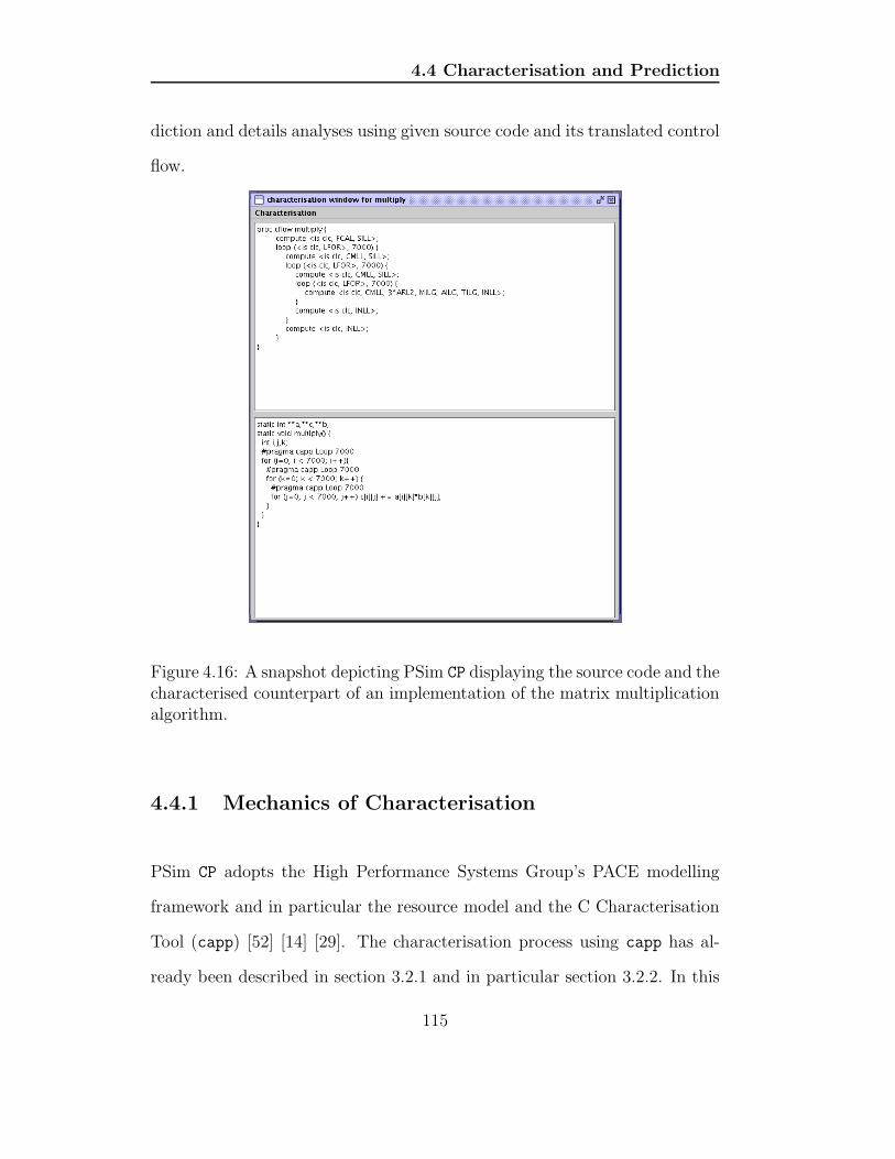
4.4 Characterisation and Prediction
diction and details analyses using given source code and its translated control
flow.
Figure 4.16: A snapshot depicting PSim CP displaying the source code and thecharacterised counterpart of an implementation of the matrix multiplicationalgorithm.
4.4.1 Mechanics of Characterisation
PSim CP adopts the High Performance Systems Group’s PACE modelling
framework and in particular the resource model and the C Characterisation
Tool (capp) [52] [14] [29]. The characterisation process using capp has al-
ready been described in section 3.2.1 and in particular section 3.2.2. In this
115

4.4 Characterisation and Prediction
section the C implementation of a matrix multiplication algorithm shown in
listing 3.4 is used as an example to describe PSim CP characterisation process.
1 proc cflow multiply {
2 compute <is clc, FCAL, SILL>;
3 loop (<is clc, LFOR>, 7000) {
4 compute <is clc, CMLL, SILL>;
5 loop (<is clc, LFOR>, 7000) {
6 compute <is clc, CMLL, SILL>;
7 loop (<is clc, LFOR>, 7000) {
8 compute <is clc, CMLL, 3*ARL2, MILG, AILG, TILG, INLL>;
9 }
10 compute <is clc, INLL>;
11 }
12 compute <is clc, INLL>;
13 }
14 }
Listing 4.27: A cflow file of the matrix multiplication algorithm from list-ing 3.4.
Unlike PACE’s performance layered models which uses the CHIP3 lan-
guage to define the application’s parallelism, the current implementation of
PSim CP focuses on sequential blocks of computations within an application,
these blocks are defined by proc cflow definitions which usually constitute
a number of processor resource usage vectors (PRUV) [53]. Each PRUV takes
the form of compute, loop, case and call which have been described dur-
ing the discussion of subtask object in section 3.2.1.2. Within each PRUV
is a collection of clcs which are translated from the C source code using
capp. Individual proc cflow is compiled into control flow files (cflow), list-
ing 4.27 shows the cflow file of the matrix multiplication algorithm shown
116

4.4 Characterisation and Prediction
in listing 3.4. PSim CP takes three types of file formats as input, they are
C source codes *.c, the corresponding control flow definition files *.cflow
and power-benchmarked hardware models cmodel of the target platforms.
This section is split into three parts: the first part describes the two types
of file inputs that PSim CP accepts (C source codes and cflow files), the
second part describes different types of resource model and their method of
constructions, and the third part documents the interpetation of inputs with
different types of resource models.
4.4.1.1 File Inputs
Apart from the necessary resource model (cmodel) for the underlying hard-
ware, PSim CP also requires the input of either a cflow file or the original C
source code modified for automatic translation.
proc cflow - A typical cflow file is shown in listing 4.27. PSim is designed
to take cflow as input and displays it on the CP interface similar to the top
part of the interface shown in figure 4.16. Without the specification of source
code only basic predictive analysis can be made and this is done by parsing
the proc cflow definition, the algorithm and generation of predictive results
are discussed in section 4.4.2.
Modified C source code - Listing 3.4 shows the original implementation
of the matrix multiplication algorithm in C. It is not possible to automate
the translation from this code into the proc cflow shown in listing 4.27,
117
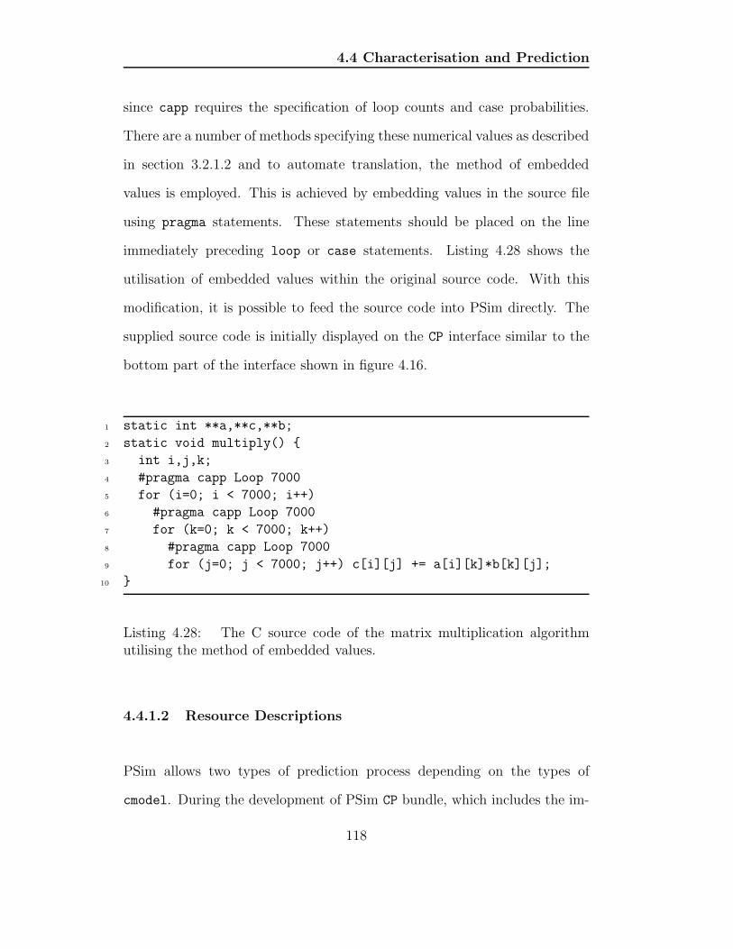
4.4 Characterisation and Prediction
since capp requires the specification of loop counts and case probabilities.
There are a number of methods specifying these numerical values as described
in section 3.2.1.2 and to automate translation, the method of embedded
values is employed. This is achieved by embedding values in the source file
using pragma statements. These statements should be placed on the line
immediately preceding loop or case statements. Listing 4.28 shows the
utilisation of embedded values within the original source code. With this
modification, it is possible to feed the source code into PSim directly. The
supplied source code is initially displayed on the CP interface similar to the
bottom part of the interface shown in figure 4.16.
1 static int **a,**c,**b;
2 static void multiply() {
3 int i,j,k;
4 #pragma capp Loop 7000
5 for (i=0; i < 7000; i++)
6 #pragma capp Loop 7000
7 for (k=0; k < 7000; k++)
8 #pragma capp Loop 7000
9 for (j=0; j < 7000; j++) c[i][j] += a[i][k]*b[k][j];
10 }
Listing 4.28: The C source code of the matrix multiplication algorithmutilising the method of embedded values.
4.4.1.2 Resource Descriptions
PSim allows two types of prediction process depending on the types of
cmodel. During the development of PSim CP bundle, which includes the im-
118

4.4 Characterisation and Prediction
plementation of the Characterisation and SourceView classes as described
briefly in appendix C, two types of cmodel were proposed, one provides a
way to model resources using elementary operations defined by clc defini-
tions and this includes operations such as ANDL and SILL, an excerpt of such
model is shown in listing 3.12. Another type, which is still in development
and is subject to future work, defines a single unit of computation by an ar-
bitary number of clc, forming “opcode chains”, this method allows resource
models to be constructed without overhead problems and while the accuracy
of power measurement remains an issue when modelling the resources of the
target platform and this is primarily caused by the experimental noise floor as
discussed in section 3.3.4, nevertheless the proposed opcode chaining method
is an attempt to minimise inaccuracies by using larger units of computation.
1 Opname,Opcode,Current,Power
2 Looping (ForLoop),SILG;LFOR;CMLG;INLG,2.46,34.39
3 Assign Array Global,ARL1;ARL1;TILG,2.08,29.17
4 Assign Array Local,ARL1;ARL1;TILL,2.08,29.17
5 Arithmetic (DoubleDivide),DFDG;TFDG,1.31,18.32
6 Arithmetic (DoubleAdd),AFDG;TFDG,1.32,18.46
7 Arithmetic (DoubleMult),MFDG;TFDG,1.27,17.83
8 Arithmetic (FloatAdd),AFSG;TFSG,1.3,18.25
9 Arithmetic (FloatDivide),DFSG;TFSG,1.79,25.13
10 Arithmetic (FloatMult),MFSG;TFSG,1.84,25.82
11 Arithmetic (IntAdd),AILG;TILG,1.99,27.9
12 Arithmetic (IntDivide),DILG;TILG,1.6,22.43
13 Arithmetic (IntMult),MILG;TILG,1.95,27.32
Listing 4.29: An excerpt of the power-benchmarked hardware object usingopcode chaining method. It uses comma separated values (csv) format toorganise resource modelling data.
119

4.4 Characterisation and Prediction
Listing 4.29 is an excerpt of the power-benchmarked hardware object using
opcode chaining method.
4.4.1.3 Characterisation Process Routine
Translation
Intermediate
Chaining
Token Parsing
{C source code}
Calculation
{Predicted Energy Consumption}
Figure 4.17: A conceptual diagram of PSim CP characterisation process rou-tine.
Figure 4.17 is the conceptual diagram of PSim CP characterisation process
routine. Prediction commences as the source code enters the routine as shown
in the figure, the inputted source code is then translated into correspond-
ing proc cflow by invoking the method createCFlowTemp() in the class
Characterisation which calls an external command shown below6.
capp -z -n source_code_modified_with_embedded_values.c
6Note that translation can only take place if capp is installed, otherwise translationcan be omitted by inputting the cflow file directly into PSim.
120

4.4 Characterisation and Prediction
proc cflow mmultiply { compute <is clc, FCAL, SILL>;
loop (<is clc, LFOR>, 7000) { compute <is clc, CMLL, SILL>;
loop (<is clc, LFOR>, 7000) { compute <is clc, CMLL, SILL>;
loop (<is clc, LFOR>, 7000) compute <is clc, CMLL, 3*ARL2,
MILG, AILG, TILG, INLL>; }
compute <is clc, INLL>; }
compute <is clc, INLL>; }
}
static int **a,**c,**b;
static void mmultiply() {
int i,j,k;
#pragma capp Loop 7000
for (i=0; i < 7000; i++) {
#pragma capp Loop 7000
for (k=0; k < 7000; k++) {
#pragma capp Loop 7000
for (j=0; j < 7000; j++) {
c[i][j] += a[i][k]*b[k][j];
}
}
}
}
mmultiply(void) C code mmultiply proc cflow
Figure 4.18: A direct mapping of C source code of matrix multiplicationalgorithm with its associated proc cflow translated code.
PSim’s CP employs a token parsing alogrithm coupled by a hash table
data structure which parses the translated code as tokens7. These tokens are
then arranged to generate a token set for the translated code. Since the class
Characterisation implements java.lang.Runnable, token parsing can be
animated. During animation PSim notifies the user about the current status
of token parsing, and with the presence of the modified source code, similar
7More information about Characterisation can be found in appendix C
121

4.4 Characterisation and Prediction
to the example shown in figure 4.16, details of token parsing can then be
directly related to the corresponding source code providing information such
as the direct mapping between the control flow definition and the C source
code, an example of which is shown in figure 4.18. With this mapping a user
can locate a “hot spot” area of the supplied source code and hence target
optimisation accordingly.
Once the complete set of tokens is retrieved from the translated code, de-
pending on whether the clc or opcode chain is used as units of computation
for the target platform, the intermediate process will be different. If opcode
chains are used, then a “chaining process” is applied to “chain” each selec-
tion of individual clcs according to the power-benchmarked hardware object
created by the opcode chaining method. Once inidividual clcs are chained,
and stored as a data structure in PSim, this data structure is subsequently
submitted for the predictive analyses and energy consumption prediction.
Predictive analyses are described in section 4.4.2.
1 Name: multiply
2 Characterised(%): 100
3 Elementary Code: 3087196028002
4 Redundant Code: 0
5 Average Current(A): 1.357805
6 Average Power(W): 26.16498
7 Time(us): 1711881719.862916
8 Total Energy(J): 57671.931927
9 Total Energy (Wms): 57671931.926515
10 Total Energy(Wus): 57671931926.51524
Listing 4.30: A summary set generated by PSim analysing translated codeof matrix multiplication algorithm shown in listing 4.28.
122
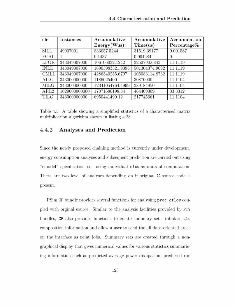
4.4 Characterisation and Prediction
clc Instances Accumulative Accumulative AccumulationEnergy(Wus) Time(us) Percentage%
SILL 49007001 833057.5244 31519.39177 0.001587FCAL 1 0.1437 0.004284 0LFOR 343049007000 106106032.1242 3252790.6843 11.1119INLL 343049007000 16903983521.9395 501304374.9092 11.1119CMLL 343049007000 4286340255.6797 105083114.8732 11.1119AILG 343000000000 1186025400 30870000 11.1104MILG 343000000000 12341054764.4999 389184950 11.1104ARL2 1029000000000 17071686198.84 464409309 33.3312TILG 343000000000 6950441499.12 217745661 11.1104
Table 4.5: A table showing a simplified statistics of a characterised matrixmultiplication algorithm shown in listing 4.28.
4.4.2 Analyses and Prediction
Since the newly proposed chaining method is currently under development,
energy consumption analyses and subsequent prediction are carried out using
“cmodel” specification i.e. using individual clcs as units of computation.
There are two level of analyses depending on if original C source code is
present.
PSim CP bundle provides several functions for analysing proc cflow cou-
pled with orginal source. Similar to the analysis facilities provided by PTV
bundles, CP also provides functions to create summary sets, tabulate clc
composition information and allow a user to send the all data-oriented areas
on the interface as print jobs. Summary sets are created through a non-
graphical display that gives numerical values for various statistics summaris-
ing information such as predicted average power dissipation, predicted run
123

4.4 Characterisation and Prediction
matrixmultiply.c
linenumber Accumulative Accumulative AccumulationEnergy(Wus) Time(us) Percentage%
2 0.1614 0.0049 6.4783E-114 705.7214 16.9419 9.0697E-75 4940049.9623 118593.9160 0.00636 5.7666E10 1.7117E9 99.9936
Table 4.6: A table showing the output of the analysis of the relation betweenstatistics shown in table 4.5 and the original source code.
time and predicted energy consumption. Figure 4.19 shows PSim displaying
the statistical summary after executing the characterisation process routine.
Listing 4.30 shows the summary set generated by PSim analysing translated
code of matrix multiplication algorithm.
Figure 4.19: A snapshot depicting PSim displaying the statistical summaryafter executing the characterisation process routine on matrix multiplicationalgorithm.
CP also generates a more detail statistical summary of the translated code,
tables 4.5 and 4.6 show the outputs of statistical summaries of the matrix
multiplication algorithm providing information such as predictive energy con-
124

4.5 Summary
sumption and run time, the composition of the algorithm in terms of clcs,
predictive energy consumption of the total number of instances of individual
clcs of which the algorithm is composed of and the distribution of the algo-
rithm’s energy consumption over its source code’s segments (line numbers).
PSim also provides functionalities for segment analysis which provides the
statistical summary of indivdual segments of the original source code. This
is achieved by utilising the direct mapping concept depicted in figure 4.18.
Listing 4.31 shows the output of the segment analysis of the ninth line of the
matrix multiplication algorithm with the corresponding statistical summary
using the direct mapping technique. These statistics allow user to have a de-
tail understanding of the energy consumption distribution of the algorithm.
1 Line Number: 9
2 Accum Energy(Wus): 5.766699117067E10
3 Accum Time(us): 1.711763109E9
4 Accum %: 99.99365028977033
5 Segment: for(j=0; j<7000; j++) c[i][j]+=a[i][k]*b[k][j];
Listing 4.31: A table showing the output of the segment analysis at ninthline of the matrix multiplication algorithm against statistical summary usingdirect mapping technique.
4.5 Summary
This chapter discussed the motivation and development of software visu-
alisation for sequential and parallel computations, using examples such as
125

4.5 Summary
ParaGraph [48] and SeeSoft [27] [26]. Based on this motivation the chapter
further described the creation and development of The Power Trace Simula-
tion and Characterisation Tools Suite (PSim). PSim is split into two bundles
- Power Trace Visualisation PTV and Characterisation and Prediction CP.
PTV provides graphical visualisation of trace data collected after monitor-
ing the power dissipation and resource usage of an application and details
these results through animation and statisitcal analyses. Coupled with this
bundle is a Perl script PComposer which provides automatic encapsulation
of the recorded data from monitoring a particular application into the cor-
responding trace file. This chapter also introduced container - a workload
coordination program and ccp - work load resource usage monitor, both
of which provides functionalities to allow selected workloads to be directly
power-benchmarked for the construction of the classification model.
CP provides characterisation and prediction functionalities. Its character-
isation methodology adopts proc cflow and clc definitions which is based
on the High Performance Systems Group’s PACE modelling framework. CP
employs the Characterisation Routine Process and utilises a novel power-
benchmarked hardware model (cmodel) which is based on the hardware
object definition in PACE and it describes the energy characterisation of
the underlying platform. The routine process uses the C Characterisation
Tool (capp) to translate C source code into a corresponding proc cflow
definition. The Characterisation Routine Process implements the concept of
application-level characterisation and energy consumption prediction method-
126

4.5 Summary
ology and presents statistical summaries including the analysis of the sup-
plied application’s composition in terms of clcs, its predicted average power
dissipation, run time and energy consumption.
The following chapter documents the results obtained from predicting the
energy consumption of several selected workloads using the characterisation
and prediction technique described so far in this thesis. The energy con-
sumption of a selection of kernels chosen from the Java Grande Benchmarks
Suite [13] are predicted using PSim. Their results are evaluated according to
size of data set and against measured consumption value.
127

Chapter 5
The Energy Consumption
Predictions of Scientific Kernels
5.1 Introduction
Previous chapters have introduced a novel application level characterisation
and energy consumption prediction technique, which uses PACE’s control
flow definition and its concept of creating resource models for the underlying
platforms. Chapter 4 has documented the implementation of PSim, a tool
suite that provides “post-processing” graphical visualisation of trace data
collected from monitoring an application’s energy consumption and resource
utilisations during its execution. PSim PTV employs a “playback” mechanism
to allow renactment of the application’s resource utilistations (including en-
128

5.2 Predictive Hypothesis
ergy) by processing trace data. PSim also provides functionalities to produce
statistical summaries of the trace data. The PSim CP bundle is designed to
execute the Characterisation Routine Process, and produce predictive results
for an application’s energy consumption and other performance metrics.
This chapter documents the evaluation of the characterisation and energy
consumption prediction technique described in this thesis and introduces a
simple mathematical model to describe the inherited inaccuracy of both the
predicted and measured energy consumptions of an application. The in-
herited inaccuracy has been documented in section 4.3. We have chosen
three processor-intensive and memory-demanding scientific kernels from the
C translation of the Java Grande Benchmark Suite [13] as the model’s train-
ing set and used a forth kernel for the model’s verification and evaluation.
5.2 Predictive Hypothesis
As explained in section 4.3, the measured energy consumptions obtained
by the black-box method described in this thesis are not accurate due to
the complex configurations of modern hardware components. Moreover the
energy consumption prediction technique described in this thesis requires
individual clc’s energy consumption to be measured, hence these predictive
values should be taken as guidelines. Meanwhile, although the proposed
prediction technique does not yield accurate results, these predictive values
are still dependable. This is because the inherited inaccuracy is consistent
129

5.2 Predictive Hypothesis
across both predicted and measured energy consumption as explained in
section 4.3.
However, in the domains of performance modelling it is possible to de-
scribe this inherited inaccuracy using a simple mathematical model. Based
on the reasons that drive this inherited inaccuracy we have proposed and fo-
rumalted an “experimental proportional relationship” linear model between
the predicted and measured energy consumption of an application. This
linear model is shown in equation 5.1 and it is a simple mathematical equa-
tion where Me is the measured energy consumption, Pe is the predicted
energy consumption, k is the proportionality constant and c is the uncer-
tainty. While the proportionality constant should be constant, the absolute
value of the uncertainty c should at most be 1
2Pe.
Me = k.Pe + c (5.1)
To acquire the optimal k and c during the model’s training, two simple
algorithms have been chosen. These algorithms are shown in equation 5.2.
k is defined to be the mean average of x where x is Me
Pebefore applying
the model shown in equation 5.1, n is the number of sets of data, c is the
product of p and ymax, and y is as the difference between the predicted and
the measured energy consumptions of the kernel after apply the model with
c = 0. ymax is the maximum of all ys within the training set and p is a factor
to be calculated during the model’s training to minimise the percentage errors
130

5.3 Model’s Training and Evaluation
between the predicted and the measured energy consumptions of the kernel
after applying the model.
k =1
n
n∑
i=1
xi
c = p.ymax (5.2)
5.3 Model’s Training and Evaluation
Four scientific kernels from the Java Grande Benchmark Suite are chosen
for the model’s training and evaluation. These kernels are popular resources
within the high-performance community for evaluating the performance of
scientific applications and they are also the workloads for constructing the
power classification’s “basic model” which has already been discussed in
section 3.3. The benchmarks chosen include Sparse Matrix Multiply, Fast
Fourier Transform and Heap Sort Algorithm from the kernels section and
Computational Fluid Dynamics from the large scale applications section.
These algorithms are evaluated with changes to the data size 1.
Note that the implementations of these scientific kernels are not identical
to the ones provided by the benchmark suite, this is because while the origi-
nal benchmark workloads are often implemented into multiple methods, the
energy consumption prediction technique described in this thesis is currently
1C source codes of related algorithms are documented in appendix D
131

5.3 Model’s Training and Evaluation
designed to accept single method applications only and it requires users to
embed pragma statements for loop counts and case probabilities. An exam-
ple of the alteration is shown in figures 5.32 and 5.33. Figure 5.32 shows
the original implementation of the heap sort algorithm in the Java Grande
Benchmark Suite and it is implemented using multiple methods. To predict
the energy consumption of this algorithm, methods heapsort and sift are
merged into a single method as shown in figure 5.33. Figure 5.33 also depicts
the pragma statements being embedded into the algorithm’s source code.
1 static int *TestArray;
2 static int rows;
3 void heapsort() {
4 int temp,i;
5 int top = rows - 1;
6
7 for (i = top/2; i > 0; --i)
8 sift(i,top);
9
10 for (i = top; i > 0; --i) {
11 sift(0,i);
12 temp = TestArray[0];
13 TestArray[0] = TestArray[i];
14 TestArray[i] = temp;
15 }
16 }
17
18 void sift(int min, int max) {
19 int k;
20 int temp;
21
22 while((min + min) <= max) {
23 k = min + min;
24 if (k < max)
25 if (TestArray[k] < TestArray[k+1]) ++k;
26 if (TestArray[min] < TestArray[k]) {
132

5.3 Model’s Training and Evaluation
27 temp = TestArray[k];
28 TestArray[k]
29 = TestArray[min];
30 TestArray[min] = temp;
31 min = k;
32 } else min = max + 1;
33 }
34 }
Listing 5.32: The original implementation of heap sort algorithm in the JavaGrande Benchmark Suite.
1 static int *TestArray;
2 static int rows;
3 void heapsort() {
4 int temp,i,k,ti,min;
5 int top = rows - 1;
6
7 #pragma capp Loop 500000
8 for (i = top/2; i > 0; --i) {
9 ti = i;
10 #pragma capp Loop 2
11 while((ti + ti) <= top) {
12 k = ti + ti;
13 #pragma capp If 0.5
14 if (k < top) {
15 #pragma capp If 0.5
16 if (TestArray[k] < TestArray[k+1]) ++k;
17 }
18 #pragma capp If 0.5
19 if (TestArray[ti] < TestArray[k]) {
20 temp = TestArray[k];
21 TestArray[k] = TestArray[ti];
22 TestArray[ti] = temp;
23 ti = k;
24 } else ti = top + 1;
25 }
26 }
133

5.3 Model’s Training and Evaluation
27
28 #pragma capp Loop 999999
29 for (i = top; i > 0; --i) {
30 min = 0;
31 #pragma capp Loop 18
32 while((min + min) <= i) {
33 k = min + min;
34 #pragma capp If 0.5
35 if (k < i) {
36 #pragma capp If 0.5
37 if (TestArray[k] < TestArray[k+1]) ++k;
38 }
39 #pragma capp If 0.5
40 if (TestArray[min] < TestArray[k]) {
41 temp = TestArray[k];
42 TestArray[k] = TestArray[min];
43 TestArray[min] = temp;
44 min = k;
45 } else min = i + 1;
46 }
47
48 temp = TestArray[0];
49 TestArray[0] = TestArray[i];
50 TestArray[i] = temp;
51 }
52
53 }
Listing 5.33: The single method implementation of heap sort algorithm withpragma statements embedded for loop counts and case probabilities.
The performance-critical section of each kernel is characterised into proc
cflow and evaluated over a range of data varing in size in order to predict
its energy consumption prior to execution; any initialisation of data or final
verification is therefore not characterised within these experiments.
The remaining chapter consists four sections: the first three sections docu-
134

5.4 Sparse Matrix Multiply
ment the evaluations of the Sparse Matrix Multiplication, Fast Fourier Trans-
form and Heap Sort Algorithm kernels as the model’s training sets. Subse-
quently the training data is used to acquire a predictive model for the energy
consumption of an application and the Computational Fluid Dynamics kernel
is chosen for the model’s evaluation. Predictive energy consumptions are veri-
fied with the measured energy consumption of these kernels on a Fedora Linux
Core 3 workstation named ip-115-69-dhcp containing a 2.8GHz Intel Pen-
tium IV processor and 448 MBs RAM. Similar to the case study documented
in chapter 1 this experiment uses a METRA HIT 29S Precision Digital Mul-
timeter to measure and record the current in ampere drawn through the
main electricity cable and the voltage acrossed it. They are measured at an
interval of 50 milliseconds. The data is captured using the BD232 Interface
Adaptor that connects to a workstation running METRAwin10/METRAHit
which processes and archives the raw data from the meter into ASCII values
for further processing [47]. A C function gettimeofday() is used to record
each kernel’s run time in milliseconds2.
5.4 Sparse Matrix Multiply
The sparse matrix multiplication from Java Grande Benchmark Suite is
adapted from the sequential Scimark benchmark that calculates the func-
2The benchmarked energy consumption for each clc computation is calculated usingthe described experimental setup and the equation 1.2 provided in chapter 1. A copyof the power benchmarked hardware model describing ip-115-69-dhcp can be found inappendix E
135

5.4 Sparse Matrix Multiply
tion y = Ax. A is an unstructured sparse matrix of size NxN , stored in
compressed-row format with a prescribed sparsity structure of nz non-zero
values. y is a Mx1 vector and x is a 1xN vector. M , N and nz are parame-
ters, where M must equal N for all benchmark executions.
1 static double *x,*y,*val;
2 static int *col,*row;
3
4 static void sparsematmult(void) {
5 int reps,SPARSE_NUM_ITER,i,nz;
6
7 for (reps=0; reps<SPARSE_NUM_ITER; reps++) {
8 for (i=0; i<nz; i++) y[ row[i] ] += x[ col[i] ] * val[i];
9 }
10 }
Listing 5.34: sparsematmult - the evaluated section of the sparse matrixmultiplication.
1 proc cflow sparsematmult {
2 compute <is clc, FCAL, SILL>;
3 loop (<is clc, LFOR>, 200) {
4 compute <is clc, CMLL, SILL>;
5 loop (<is clc, LFOR>, 250000) {
6 compute <is clc, CMLL, 3*ARD1, MFDG, AFDG, TFDG, INLL>;
7 }
8 compute <is clc, INLL>;
9 }
10 }
Listing 5.35: The characterised proc cflow definition of the sparsematmultrunning dataset 50000X50000 shown in listing 5.34.
136

5.4 Sparse Matrix Multiply
Dataset Measured Predicted PercentageEnergy(J) Energy(J) Error(%)
50000X50000 336.5247 273.8570 18.62100000X100000 943.5225 547.7134 41.95500000X500000 6044.9850 2738.5652 54.70
Table 5.1: A table showing the predicted energy consumption against themeasured energy consumption of sparsematmult on ip-115-69-dhcp, theforth column shows the percentage error between the measured and predictedvalues.
The performance-critical element of this benchmark is implemented in
the method sparsematmult which performs the multiplication and updates
the result to the vector y. The segments of source code which include the
matrix initialisation and the multiplication sections of this benchmark are
shown in appendix D. Listings 5.34 and 5.35 show the evaluated section of
the benchmark sparsematmult and its proc cflow definition respectively.
Three sets of data are chosen during this kernel’s evaluation, they are
unstructured sparse matrices of size NxN where N are 50000, 100000 and
5000000. For each size of data set, the average execution time and energy
consumption are measured over 10 iterations where in each iteration multi-
plications are carried out 200 times. Table 5.1 shows the comparative results
between measured and predicted energy consumption for each sets of data.
This table contains a percentage error column showing the deviation of mea-
sured and predicted values. Figure 5.1 shows a graphical representation of
the measured and predicted energy consumption presented in table 5.1. The
range of predictive inaccuracies achieved from analysing this benchmark is
between 18.62% and 54.70%. Figure 5.1 also suggests the difference between
137

5.4 Sparse Matrix Multiply
Figure 5.1: A line graph showing the measured and predicted energy con-sumptions of sparsematmult benchmark with N set to 50000, 100000 and500000, all energy values are in joules.
the predicted and measured energy consumption increases as the size of data
set increases. This is because as the size of data set increases, the number
of clcs within the looping construct shown in listing 5.35 also increases and
this leads to an accumulative increase in the inaccuracies of clc’s energy con-
sumption. This results in the increase in the difference between the predicted
and measured energy consumption.
To optimise the required parameter k in the model described in equa-
tion 5.1, k is calculated to be 1.71962 as specified in equation 5.2. Fig-
ure 5.2 shows a line graph representing the measured and predicted energy
138

5.4 Sparse Matrix Multiply
Figure 5.2: A line graph showing the measured and predicted energy con-sumptions of sparsematmult benchmark after applying equation 5.1 withk = 1.7196 and c = 0.
consumptions of sparsematmult benchmark after applying the linear model
with k = 1.7196 and c = 0.
Figure 5.3 shows a line graph representing the measured and predicted
energy consumption of sparsematmult benchmark after applying the linear
model with k = 1.7196 and c = −89.6026. In this set, ymax is calculated to
be -134.4040 and this is the difference between the measured and predicted
energy consumptions of sparsematmult with N = 50000 and k = 1.7196. p
is set to be 2
3, this is experimentally verified to be the optimal scale factor.
Table 5.2 shows the predicted and the measured energy consumptions of
139

5.4 Sparse Matrix Multiply
Figure 5.3: A line graph showing the measured and predicted energy con-sumptions of sparsematmult benchmark after applying equation 5.1 withk = 1.7196 and c = −89.6026.
the kernel after the linear model with k = 1.7196 and c = −89.6026, the
forth column of the table shows the percentage errors between predicted and
measured values. After applying the proposed model, the range of predictive
inaccuracies achieved from analysing this benchmark is between 9.67% and
23.59%.
140

5.5 Fast Fourier Transform
Dataset Measured Predicted PercentageEnergy(J) Energy(J) Error(%)
50000X50000 336.5247 381.3260584 13.31100000X100000 943.5225 852.2537217 9.67500000X500000 6044.9850 4619.67606 23.59
Table 5.2: A table showing the predicted energy consumption against themeasured energy consumption of sparsematmult on ip-115-69-dhcp afterapplying equation 5.1 with k = 1.7196 and c = −89.6026, the forth columnshows the percentage error between the measured and predicted values.
5.5 Fast Fourier Transform
The Fast Fourier Transform performs one-dimensional forward transform of
N complex data points (number). Inside this kernel complex data is repre-
sented by 2 double values in sequence: the real and imaginary parts. N data
points are represented by a double array dimensioned to 2xN . To support
2D and subsequently higher transforms, an offset, i0 (where the first element
starts) and stride (the distance from the real part of one value, to the next:
at least 2 for complex values) can be supplied. The physical layout in the
array data, of the mathematical data d[i] is as follows:
Re(d[i]) = data[i0 + stride.i]
Im(d[i]) = data[i0 + stride.(i + 1)]
The transformed data is returned in the original data array in wrap-
141
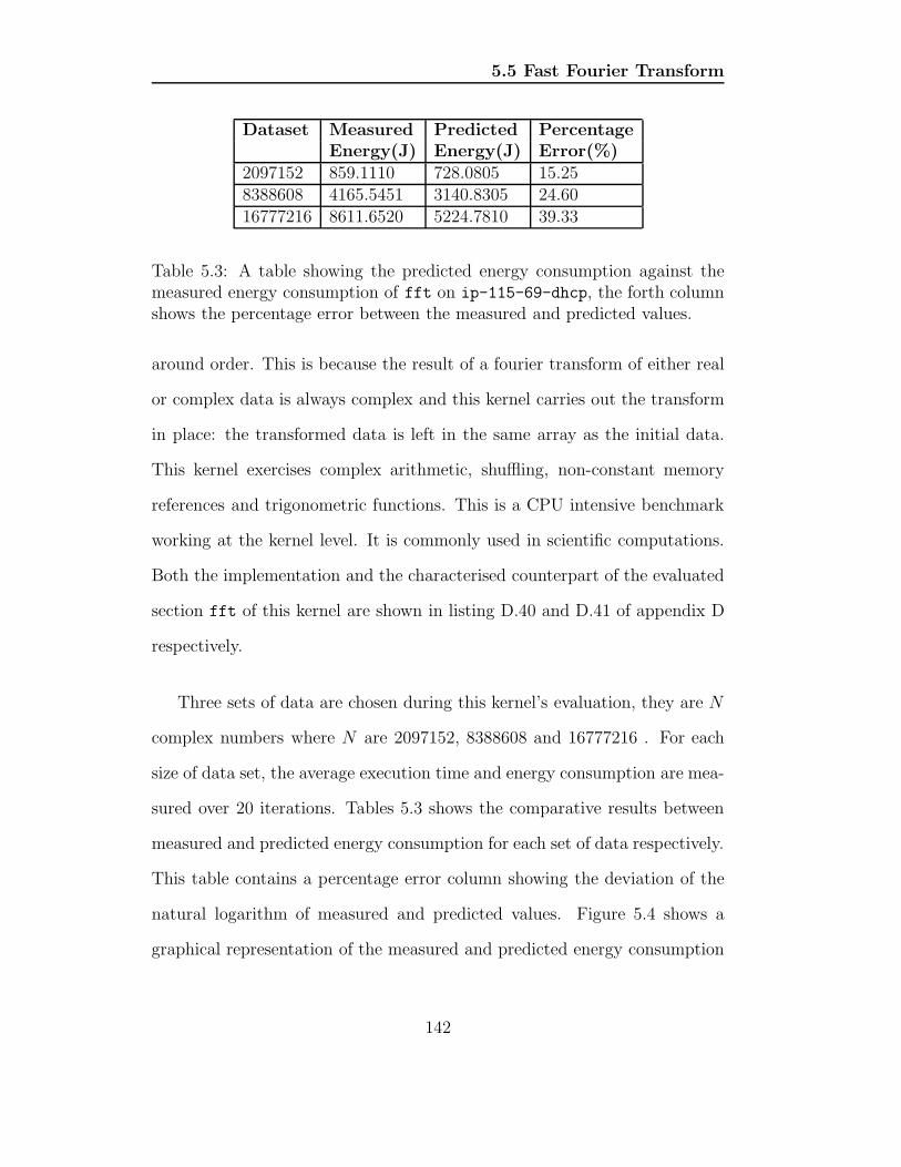
5.5 Fast Fourier Transform
Dataset Measured Predicted PercentageEnergy(J) Energy(J) Error(%)
2097152 859.1110 728.0805 15.258388608 4165.5451 3140.8305 24.6016777216 8611.6520 5224.7810 39.33
Table 5.3: A table showing the predicted energy consumption against themeasured energy consumption of fft on ip-115-69-dhcp, the forth columnshows the percentage error between the measured and predicted values.
around order. This is because the result of a fourier transform of either real
or complex data is always complex and this kernel carries out the transform
in place: the transformed data is left in the same array as the initial data.
This kernel exercises complex arithmetic, shuffling, non-constant memory
references and trigonometric functions. This is a CPU intensive benchmark
working at the kernel level. It is commonly used in scientific computations.
Both the implementation and the characterised counterpart of the evaluated
section fft of this kernel are shown in listing D.40 and D.41 of appendix D
respectively.
Three sets of data are chosen during this kernel’s evaluation, they are N
complex numbers where N are 2097152, 8388608 and 16777216 . For each
size of data set, the average execution time and energy consumption are mea-
sured over 20 iterations. Tables 5.3 shows the comparative results between
measured and predicted energy consumption for each set of data respectively.
This table contains a percentage error column showing the deviation of the
natural logarithm of measured and predicted values. Figure 5.4 shows a
graphical representation of the measured and predicted energy consumption
142
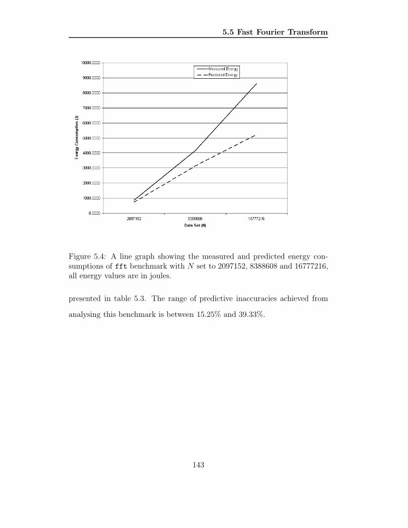
5.5 Fast Fourier Transform
Figure 5.4: A line graph showing the measured and predicted energy con-sumptions of fft benchmark with N set to 2097152, 8388608 and 16777216,all energy values are in joules.
presented in table 5.3. The range of predictive inaccuracies achieved from
analysing this benchmark is between 15.25% and 39.33%.
143

5.5 Fast Fourier Transform
Figure 5.5: A line graph showing the measured and predicted energy con-sumptions of fft benchmark with after applying equation 5.1 with k =1.3848 and c = 0.
To optimise the required parameter k in the model described in equa-
tion 5.1, k is calculated to be 1.3848 as specified by equation 5.2. Figure 5.5
shows a line graph representing the measured and predicted energy con-
sumptions of fft benchmark after applying equation 5.1 with k = 1.3848
and c = 0.
144

5.6 Heap Sort Algorithm
Dataset Measured Predicted PercentageEnergy(J) Energy(J) Error(%)
2097152 859.1110 1022.0220 18.968388608 4165.5451 4363.2426 4.7516777216 8611.6520 7249.1354 15.82
Table 5.4: A table showing the predicted energy consumption against themeasured energy consumption of fft on ip-115-69-dhcp after applyingequation 5.1 with k = 1.3848 and c = 13.7628, the forth column showsthe percentage error between the measured and predicted values.
Figure 5.6 shows the line graph representing the measured and predicted
energy consumptions of fft benchmark after applying equation 5.1 with
k = 1.3848 and c = 13.7628. In this training set, ymax is calculated to
be 1376.2794 while p is calculated to be 0.01. ymax is calulated the differ-
ence between the measured and predicted energy consumption of fft with
N = 16777216 and k = 1.3848 while p is 0.01 as it has been experimentally
verified to be the optimal scale factor. Table 5.4 shows the predicted and the
measured energy consumptions of the kernel after applying equation 5.1 with
k = 1.3848 and c = 13.7628, the forth column of the table shows the per-
centage errors between predicted and measured values. After applying the
proposed model, the range of predictive inaccuracies achieved from analysing
this benchmark is between 4.75% and 18.96%.
5.6 Heap Sort Algorithm
Heap sort is a member of the family of selection sorts. This family of al-
gorithms works by determining the largest (or smallest) element of the list,
145
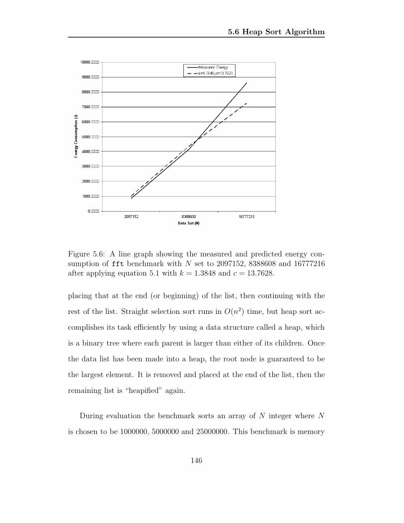
5.6 Heap Sort Algorithm
Figure 5.6: A line graph showing the measured and predicted energy con-sumption of fft benchmark with N set to 2097152, 8388608 and 16777216after applying equation 5.1 with k = 1.3848 and c = 13.7628.
placing that at the end (or beginning) of the list, then continuing with the
rest of the list. Straight selection sort runs in O(n2) time, but heap sort ac-
complishes its task efficiently by using a data structure called a heap, which
is a binary tree where each parent is larger than either of its children. Once
the data list has been made into a heap, the root node is guaranteed to be
the largest element. It is removed and placed at the end of the list, then the
remaining list is “heapified” again.
During evaluation the benchmark sorts an array of N integer where N
is chosen to be 1000000, 5000000 and 25000000. This benchmark is memory
146

5.6 Heap Sort Algorithm
Dataset Measured Predicted PercentageEnergy(J) Energy(J) Error(%)
1000000 58.2667 53.5485 8.105000000 447.9064 307.4212 31.3625000000 3080.9534 1669.3671 45.82
Table 5.5: A table showing the predicted energy consumption against themeasured energy consumption of heapsort on ip-115-69-dhcp, the forthcolumn shows the percentage error between the measured and predicted val-ues.
and integer intensive. Both implementation and characterised counterpart
of the evaluated section heapsort of this kernel are shown in listing D.38
and D.39 of appendix D respectively.
Three sets of data are chosen during this kernel’s evaluation, they are
integer arrays of length N where N are 1000000, 5000000 and 25000000 For
each size of data set, the average execution time and energy consumption are
measured over 20 iterations. Unlike previous discussed kernels, due to the
nature of sorting algorithms, both execution time and energy consumption
are highly data dependent. Therefore for every iteration of the sort, data
must be re-initialised.
Listing 5.36 shows the implementation of the method initialise which
is responsible for creating the required integer array. During the evaluation
of the method heapsort, initialise must be called prior the execution of
heapsort to ensure consistency of unsorted data. Therefore to evaluate this
kernel in conformance with the rest of the kernel evaluations in this chapter,
the execution time and energy consumption of the method initialise are
147

5.6 Heap Sort Algorithm
Figure 5.7: A line graph showing the measured and predicted energy con-sumptions of heapsort benchmark with N set to 1000000, 5000000 and25000000, all energy values are in joules.
measured, calculated and used as the overhead for the kernel so that only
the operations within heapsort are accounted for.
Tables 5.5 shows the comparative results between measured and predicted
energy consumption of the kernel for all three sets of data. This table con-
tains a percentage error column showing difference between measured and
predicted values. Figure 5.7 shows a graphical representation of the mea-
sured and predicted energy consumptions presented in table 5.5. The range
of predictive inaccuracies achieved from analysing this benchmark is between
8.10% and 45.82%. To optimise the required parameter k in the linear model,
148

5.6 Heap Sort Algorithm
k is calculated to be 1.4636. Figure 5.8 shows a line graph representing the
measured and predicted energy consumptions of heapsort benchmark after
applying the linear model with k = 1.4636 and c = 0.
1 static int rows;
2 static int *array;
3
4 static void initialise() {
5 int i;
6 array = (int *) malloc(sizeof(int) * rows);
7 rinit(1729);
8 for(i = 0; i < rows; i++) {
9 array [i] = (int) (uni() * 2147483647);
10 }
11 }
Listing 5.36: initialise - a method used to create integer array for heapsort algorithm kernel.
Figure 5.9 shows the line graph representing the measured and predicted
energy consumption of heapsort benchmark after applying equation 5.1 with
k = 1.4636 and c = −18.2770. In this training set, ymax is calculated to be
-20.1047 while p is calculated to be 1
1.1. ymax in this training set is the differ-
ence between the measured and predicted energy consumption of heapsort
with N = 1000000 and k = 1.4636, this is because the largest percentage
error after acquiring k is the measured and predicted energy consumption
of the kernel with N = 1000000, while p is calculated 1
1.1as it has been
experimentally verified to be the optimal scale factor. Table 5.6 shows the
predicted and the measured energy consumptions of the kernel after applying
equation 5.1 with k = 1.4636 and c = −18.2770, the forth column of the table
149

5.6 Heap Sort Algorithm
Figure 5.8: A line graph showing the measured and predicted energy con-sumption of heapsort benchmark with after applying equation 5.1 withk = 1.4636 and c = 0.
shows the percentage errors between predicted and measured values. After
applying the proposed model, the range of predictive inaccuracies achieved
from analysing this benchmark is between 3.14% and 21.29%.
150

5.7 Model’s Verification and Evaluation
Figure 5.9: A line graph showing the measured and predicted energy con-sumption of heapsort benchmark with after applying equation 5.1 withk = 1.4636 and c = −18.2770.
5.7 Model’s Verification and Evaluation
The previous three sections described the training sets for the proposed “ex-
perimental proportional relationship” linear model, three kernels from the
Java Grande Benchmark Suite, namely Sparse Matrix Multiply, Fast Fourier
Transform and Heap Sort Algorithm, were used to train both k and c for
model optimisation. Table 5.7 shows the k and c values used during the en-
ergy consumption prediction and evaluations of the three kernels described
in previous sections. These values were calculated based on the percentage
differences between the predicted and the measured energy consumptions of
151

5.7 Model’s Verification and Evaluation
Dataset Measured Predicted PercentageEnergy(J) Energy(J) Error(%)
1000000 58.2667 60.0944 3.145000000 447.9064 431.6514 3.6325000000 3080.9534 2424.9368 21.29
Table 5.6: A table showing the predicted energy consumption against themeasured energy consumption of heapsort on ip-115-69-dhcp after apply-ing equation 5.1 with k = 1.4636 and c = −18.2770, the forth column showsthe percentage error between the measured and predicted values.
Kernels k c percentage %Sparse Matrix Multiply 1.7196 -89.6026 22.90Fast Fourier Transform 1.3848 13.7628 13.22Heap Sort Algorithm 1.4636 -18.2770 19.07
Table 5.7: A table showing the k and c values used during the energy con-sumption prediction and evaluations of the three kernels used for model’straining. The forth column is the mean average of the percentage errors ofeach kernel’s predictions after applying the proposed linear model.
the evaluated kernels, the forth column of table 5.7 shows the percentage
differences of the mean average of the percentage errors of each kernel’s pre-
dictions after applying the proposed linear model. We use the mean average
of the k and c values shown in table 5.7 to represent the proportionality
constant and the uncertainty of the linear model. Hence k is calculated to
be 1.5393 and c is calculated to be -30.3723.
A large scale application kernel from the C translation of the Java Grande
Benchmark Suite is chosen for the model’s verification and evaluation, this
is a Euler benchmark that solves time-dependent Euler equations for flow
in a channel with a “bump” on one of the walls. A structured, irregular,
152

5.7 Model’s Verification and Evaluation
Dataset Measured Predicted PercentageEnergy(J) Energy(J) Error(%)
64 471.9126 326.2020 30.8896 1003.1683 667.1780 33.49
Table 5.8: A table showing the predicted energy consumption against themeasured energy consumption of euler on ip-115-69-dhcp, the forth col-umn shows the percentage error between the measured and predicted values.
Nx4N mesh is employed, and the solution method is a finite volume scheme
using a fourth order Runge-Kutta method with both second and fourth order
damping. The solution is iterated for 200 time steps. Since the source code
of the implementation used for evaluation is around 2000 lines, it is not listed
in this thesis.
Two sets of data are chosen during this kernel’s evaluation, they are
structured, irregular, Nx4N mesh where N are 64 and 96. For each size of
data set, the average execution time and energy consumption are measured
over 10 iterations where in each iteration the specific soluation are iterated for
200 time steps. Tables 5.8 shows the comparative results between measured
and predicted energy consumption of the kernel for all two sets of data.
This table contains a percentage error column showing the differences of
measured and predicted values. Figure 5.10 shows a graphical representation
of the measured and predicted energy consumption presented in table 5.8.
The predictive inaccuracies achieved from evaluating this kernel are 13.60%
and 16.87%.
Figure 5.11 shows a line graph representing the measured and predicted
153

5.7 Model’s Verification and Evaluation
Figure 5.10: A line graph showing the measured and predicted energy con-sumptions of euler benchmark with N set to 64 and 96, all energy valuesare in joules.
energy consumption of euler benchmark after applying the linear model
with k = 1.5393 and c = 0. The predictive inaccuracies after applying the
proposed linear model with k = 1.5393 and c = 0 are 6.40% and 2.37%.
Table 5.9 shows the predicted and the measured energy consumptions of
the kernel after applying equation 5.1 with k = 1.4636 and c = −18.2770,
the forth column of the table shows the percentage errors between predicted
and measured values. A line representation of the comparison between the
measured values and the predicted values afte applying the linear model is
shown in figure 5.12. After applying the proposed model, the predictive
154

5.8 Summary
Figure 5.11: A line graph showing the measured and predicted energy con-sumption of euler benchmark with N set to 64 and 96 after applying equa-tion 5.1 with k = 1.5393 and c = 0.
inaccuracies achieved are 0.032% and 0.651%.
5.8 Summary
This chapter illustrated the usage of the energy consumption prediction
methodology described in this thesis and how this can be applied to pre-
dict the energy consumption of processor-intensive and memory-demanding
scientific applications. It documented an “experimental proportional rela-
tionship” linear model after recognising a static inaccuracy in the energy
155

5.8 Summary
Dataset Measured Predicted PercentageEnergy(J) Energy(J) Error(%)
64 471.9126 471.7613 0.03296 1003.1683 996.6371 0.651
Table 5.9: A table showing the predicted energy consumption against themeasured energy consumption of euler on ip-115-69-dhcp after applyingequation 5.1 with k = 1.5393 and c = −30.3723, the forth column shows thepercentage error between the measured and predicted values.
consumption measurement as described in section 4.3. This model is trained
with three scientific kernels from the C translation of the Java Grande Benck-
mark Suite. These kernels were characterised into control flow definitions
(proc cflow) and evaluated over a range of data varying in size. The eval-
uated energy consumption was then compared with the kernels’ measured
energy consumption during execution in order to calculate the predictions’
accuracies.
These results were applied to the proposed model in order to optimise the
model’s parameters k and c for applications executing on ip-115-69-dhcp.
The model’s parameters k and c represent the proportionality constant and
the uncertainty. The model was verified and evaluated using a large scale
application kernel from the C translation of the Java Grande Benckmark
Suite that solves time-dependent Euler equations. All benchmarks except
the heap sort algorithm contained no data-dependent elements of code and
could therefore be accurately predicted without any prior execution. Since
the heap sort algorithm is data dependant, at every iteration initialise
is invoked and its energy consumption accounted for as overhead prior ex-
156

5.8 Summary
Figure 5.12: A line graph showing the measured and predicted energy con-sumption of euler benchmark with N set to 64 and 96 after applying equa-tion 5.1 with k = 1.5393 and c = −30.3723.
ecuting the performance-critical section heapsort. The inaccuracies of the
predictive evaluations before applying the proposed model were 13.60% and
16.87% and the inaccuracies of the same predictive evaluations after apply-
ing the proposed model were 0.032% and 0.651%. This result suggested the
predicted energy consumption of an application produced by the proposed
energy consumption prediction methodology has an “experimental propor-
tional relationship” with the application’s measured energy consumption.
157

Chapter 6
Conclusion
The increase in applications’ energy consumption in modern computational
architectures has motivated the development of an analysis methodology to
characterise and predict applications’ energy consumption. By using this
technique developers and analysts can optimise an application’s energy con-
sumption accordingly. Furthermore, a disproportional relationship between
an application’s run time and energy consumption, which has been shown
by a simple case study in chapter 1, has further motivated the research in
energy consumption prediction which is documented in this thesis.
This thesis first documented a detail review of current techniques in the
power-aware computing area including power management and source code
cost analyses. These techniques were categorised into the following three
categories:
158

• Traditional and General Purposes,
• Micro and Hardware Level,
• Macro and Software Level.
The review in chapter 2 identified the shortcomings in current power
analysis techniques. Firstly, the review pinpointed the inflexibilities of these
techniques, as they either require analysers to have very detail and spe-
cific knowledge such as the low-level machine code or require them to use
specialised equipments which might not be available. Secondly, the review
suggested that these power analyses techniques have separated themselves
from the general performance domain by neglecting performance efficiency
or have isolated energy consumption completely from other performance met-
rics such as execution time or memory utilisation. This is a major concern
as the rapid increase in energy consumption meant that energy should be
included into general cost analyses for performance measures. Thirdly, the
review suggested that currrently there’s no standard model for power analy-
sis which allows application to be systematically or hierarchically optimised
for energy usage and it is believed that such standardisation is important as
applications are moving toward heterogeneous, distributed and even ubiq-
uitous platforms. Also by using an analytical model, it allows energy or
other performance measurements to be based on a hierarchical framework of
relativity.
Subsequently, following from the directions suggested in chapter 2 and
the beginning of chapter 3, in the remaining chapters 3 and 4, two method-
159

ologies and concepts in power-metric analysis and application predictions
were proposed. They include the application level analysis by characterising
applications into blocks of control flow definitions (proc cflow) and a novel
method of power analysis utilising the mapping concept of a power classifi-
cation model. These techniques are computational environment independent
since they abstract from the underlying platform using either the correspond-
ing hardware object or an instantiation of the basic model, as a result, it is
possible for applications’ energy consumption to be analysed and predicted
over all types of underlying platform.
The methodology of application level power analysis by characterising
individual applications into blocks of control flow definitions (proc cflow)
was implemented as a set of tools called the Power Trace Simulation and
Characterisation Tools Suite (PSim). This tools suite is split into two sep-
arate bundles - PTV and CP. PTV provides graphical visualisations on trace
data collected from the monitoring of power dissipation and resource usage
of a running application, and it also processes these results using animation
and statisitcal analyses, while CP provides characterisation and prediction
functionalities. Its characterisation methodology uses a control flow proce-
dure (proc cflow) and clc definitions adopted from the High Performance
Systems Group’s PACE modelling framework whose definition has been de-
scribed in chapter 3.
Chapter 5 documented the examinations of the characterisation and en-
ergy consumption prediction. This chapter introduced an “experimental pro-
160

6.1 Future Work
portional relationship” linear model after recognising a static inaccuracy in
the energy consumption measurement as described in section 4.3. The linear
model is shown in equation 5.1 and the model is trained with three scien-
tific kernels from the C translation of the Java Grande Benckmark Suite.
These kernels were characterised into control flow definitions (proc cflow)
and evaluated over a range of data varying in size. These results were ap-
plied to the proposed model in order to optimise the model’s parameters
k and c for applications executing on ip-115-69-dhcp. The model’s para-
meters k and c represent the proportionality constant and the uncertainty.
The model was verified and evaluated using a large scale application ker-
nel from the C translation of the Java Grande Benckmark Suite that solves
time-dependent Euler equations The inaccuracies of the predictive evalua-
tions before applying the proposed model were 13.60% and 16.87% while the
inaccuracies of the same predictive evaluations after applying the proposed
model were 0.032% and 0.651%. This result suggested the predicted energy
consumption of an application produced by the proposed energy consump-
tion prediction methodology has an “experimental proportional relationship”
with the application’s measured energy consumption.
6.1 Future Work
There are a number of areas of future work. They fall into three distinct
categories:
161

6.1 Future Work
1. Hardware model refinement - Since the comparison in chapter 5 showed
that the numerical values of the predictions conform to an experimen-
tal proportional relationship with the measured values, it is therefore
necessary and feasible to refine the current hardware model construc-
tion method to minimise this error. Refinements may be carried out
by more detail investigations into the behaviour of the targeted appli-
cations against the trace data collected from the corresponding power
analysis. The current methodology of power analysis using a digital
multimeter might prove to be insufficient and hence it might be neces-
sary to monitor the electrical power dissipated from different parts of
the underlying hardware components such as the CPU and the memory
chip. By having a bank of energy consumption of individual hardware
component whilst executing elementary operations, it might be possible
to construct a more accurate and complete model for energy consump-
tion prediction. Moreover, it may also be possible to extend a broader
class of experimental platforms and apply different monitoring tech-
niques such as observing the discharge from a battery of a portable
computer [41].
2. PACE Integration - The current application-level energy consumption
prediction technique is based on the characterising the target applica-
tion into blocks of control flow definitions proc flow. Therefore it is a
natural development to bring this prediction technique into the PACE
framework which uses such definition as blocks of sequential compu-
tations. To enable this integration, apart from refining the current
162

6.1 Future Work
hardware model as described above, the current energy consumption
prediction technique must be extended to allow prediction on parallel
computations such as MPI-implemented applications. Also the energy
consumption prediction can be extended for jPACE [72] (jPACE is an
extension to PACE in performance prediction for Java distributed ap-
plications). This can be achieved by investigating the energy cost of
bytecode blocks, this is a feasible extension as the performance costs of
these bytecode blocks have been investigated during the construction
of jPACE [73].
3. General cost classification model - As suggested in section 3.1, there
is a need to have a standard model for power analysis which allows
applications to be systematically or hierarchically optimised for energy
usage. Similar to the idea of PACE integration, it should be possible to
extend the power classification model concept into a more general cost
classification model, as this will allow general cost analysis to be car-
ried out relatively and it also means that measurements no longer need
to be absolute but rather they can be based on a hierarchical frame-
work of relativity. This innovative encapsulation model will also allow
performance modelling to be carried out generically as it is possible to
abstract the underlying platforms into resource models.
163

Appendix A
PComposer usage page
NAME
PComposer - PSim trace file compiler and power-benchmarked hardware
object constructor.
SYNOPSIS
./PComposer.pl [[-s|-a|-p|-w|-ah|-hmcl|-hmcl-all|-c] [tracename]] | [-h]
DESCRIPTION
PComposer extracts power and resource measurements from experimental
trace and creates (non-synchronized) simulation trace file in comma
separated values (csv) format. It uses experiment’s run time as the
pivot to merge monitored data recorded by the digital multimeter and
ccp. If container is used to monitor workload data, PComposer will
164

also carry out merges with those trace data. It also creates summary
tables with relevant HMCL opcode. PComposer also provide functionalities
to construct power-benchmarked hardware object constructor (*.cmodel)
by collecting power trace data by measuring the current drawn by the
execution of the altered version of C Operation Benchmark Program ’bench’.
EXAMPLES
./PComposer.pl -a fft_1956210105 - Compile fft_1956210105.simulate
from files in directory fft_1956210105 containing fft_1956210105.txt,
resource.dat etc.
OPTIONS
-a TRACE-NAME compiles individual trace file specified by
TRACE-NAME (*.simulate)
-ah HMCL_DIR iteratively compiles HMCL trace file (*.simulate)
-c correct HMCL out-of-sync trace file (*.simulate)
-h print this help, then exit
-hmcl compiles HMCL cmodel file for power
characterisation (*.cmodel)
-hmcl-all analyse a single hmcl power file to construct
individual power files for further analysis
-hmcl-code construct hmcl.code from output of pace/cmr/cpu/bench.c
for hmcl run time reference
-p compiles Opcode (HMCL chains) timings and construct
corresponding power value (rCurrent-NWp,rPower-NWp) (*.csv)
165

-s makes Summary file (*.summary)
-w normalises Opcode (HMCL chains) power values
from non-workload timing (*.summary)
SEE ALSO
ccp, container, PSim
AUTHOR
Peter Wong, Department of Computer Science, University of Warwick
166

Appendix B
container and ccp usage page
NAME
container, ccp - Performance benchmark workload container for classification
model and work load resource usage monitor.
SYNOPSIS
./container [[--ar|--lo|--iv|--fft|--mult|--sor|--heap|--lu|--ser|--eul|
--mol|--non|--bub] [-i iteration] [-o logfile]] [-n|--nostore] [--clean] |
[-h|--help]
./ccp [workload]
DESCRIPTION
Container executes and monitors selected workloads for constructing
167
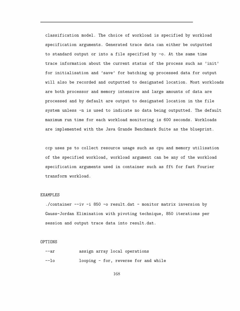
classification model. The choice of workload is specified by workload
specification arguments. Generated trace data can either be outputted
to standard output or into a file specified by -o. At the same time
trace information about the current status of the process such as ’init’
for initialisation and ’save’ for batching up processed data for output
will also be recorded and outputted to designated location. Most workloads
are both processor and memory intensive and large amounts of data are
processed and by default are output to designated location in the file
system unless -n is used to indicate no data being outputted. The default
maximum run time for each workload monitoring is 600 seconds. Workloads
are implemented with the Java Grande Benchmark Suite as the blueprint.
ccp uses ps to collect resource usage such as cpu and memory utilisation
of the specified workload, workload argument can be any of the workload
specification arguments used in container such as fft for fast Fourier
transform workload.
EXAMPLES
./container --iv -i 850 -o result.dat - monitor matrix inversion by
Gauss-Jordan Elimination with pivoting technique, 850 iterations per
session and output trace data into result.dat.
OPTIONS
--ar assign array local operations
--lo looping - for, reverse for and while
168

--iv matrix inversion by gauss-jordan elimination with pivoting
--fft Fast Fourier Transform
--mult sparse matrix multiplication
--sor successive over-relaxation
--mult sparse matrix multiplication
--heap heap sort algorithm
--lu LU factorisation
--ser fourier coefficient analysis
--eul computational fluid dynamics
--mol molecular dynamics simulation
--non no workload, benchmark container itself
--bub bubble sort algorithm
-i iteration workload Iteration
-o logfile output file
-n --nostore inhibits all processed data output (excluding trace data)
--clean empty specified data file for processed data output
-h --help print this help, then exit
TRACE FORMAT
Container outputs all trace data in comma seperated value (csv) format as it
is a de facto standard for portable representation of a database and has
been used for exchanging and converting data between various spreadsheet
programs. Below is the standard format for each piece of monitoring trace.
169

Wn,Sc,ipS,eRt,SRt,ips,ct
where Wn - Workload Name
Sc - Session counts
ipS - Iterations per sessions
eRt - execution run time
SRt - session run time
ips - average iterations per second
ct - current time
eg. fft,acc.1x100:0.390448,ses1:0.390445,aver:256.118058,tm:13:06:40.655497
SEE ALSO
PSim, PComposer, ps
AUTHOR
Peter Wong, Department of Computer Science, University of Warwick
170

Appendix C
About Java Package
uk.ac.warwick.dcs.hpsg.PSimulate
PSim’s implementation package is uk.ac.warwick.dcs.hpsg.PSimulate writ-
ten in JavaTM (J2SE version 1.4.2) and its UML class diagram is shown in
figure C.1. Not all methods and classes have been included in figure C.1,
only the most prominent information is shown. There are a number of
classes omitted in the UML diagram, they are bSemaphore, printSummary,
printTable, TraceException. Table C.1 describes individual main classes
of the package, note all nested classes, such as Simulate.SimVerifier, are
not described in this appendix.
171

Class Name Description SummarybSemaphore Provides an internal (strict) binary semaphore
used to synchronised concurrent operation such asanimated characterisation for PSim.
Characterisation Characterisation windows and functions class forPSim, carries algorithms for application predictionand provides the generation of application levelprediction result
printSummary Provides the display and manipulation of summarydata, it also provides printing capability forthese data.
printTable Provides the display and manipulation of analyseddata usually in tabular form, it also providesprinting capability for these data.
Simulate Provides graphical user interface for PSim.SimStep Provide PSim’s encapsulation for individual
trace data and provides functions to manipulate thesedata
SourceView Source code viewer and functions class for PSimand carries algorithms to generate predictionresults at source code’s line level.
Summary Provide Interface and function to interpret andverify summary datasets created by PSim
TimeChart Provides visualisation displays and animations inPSim. Provides the generation of trace analysissummary and results
Trace Provides encapsulation for Monitoring Trace Data(*.simulate) in PSim and provides functions tomanipulate and process these data
TraceException Exception class for the entire package.
Table C.1: A table describing individual main classes (excluding nestedclasses) of the package uk.ac.warwick.dcs.hpsg.PSimulate.
172

-analyseOverhead() : String[]
-analyseTrace() : File
-createAndShowGUI()
-characterCFlow() : Characterisation
-createMenu() : JMenu
-zoom()
-playSimulation()
-stopSimulation()
-pauseSimulation()
-displaySummary()
-runTrace()
-openTrace()
-closeTrace()
-saveTrace() : boolean
-buildSourceSummary()
-buildCharWindows()
-buildCharWindowsSummary()
-synWindows()
-currentTrace : String
-bfluct : int = 0
-efluct : int = 0
-bzoom : int = 0
-azoom : int = 0
-trace : Trace
Simulate
+analyse() : int
+getCPUValue() : float
+getMemValue() : float
+getPowerValue() : float
+getAccumValue() : float
+getOpsValue() : String[]
+size() : int
+synchronize() : Trace
+shiftAll() : Trace
+shiftPower() : Trace
+setUseRunTime()
-syncStart : int = 0
-syncEnd : int = 0
-defaultRunTime : float = 0.0
-defaultVoltage : float = 0.0
-overhead : float = 0.0
-useContainer : boolean = false
-useOverHead : boolean = false
-useRunTime : boolean = false
-isSync : boolean = false
-dataSet : SimStep[]
Trace
1
-contains
1
+setLineNumber()
+useOverHead()
+getTableHeading() : String[]
+getTableData() : String[][]
+startChara() : boolean
+updateTableData()
-characterise() : int
-setCurrentLine()
-debug()
-setSourceScan()
-addOpCode()
-setupChara()
-processCode() : boolean
+run()
-formatResult()
+getSummary() : String
+getEnergy() : String
+getRunTime() : String
+getSource() : File
+getCFlow() : File
+getCModel() : File
+createCFlow()
+formatSourceResult()
+createCFlowTemp()
+createInterface()
+loadSourceCode() : boolean
+setAnimated() : boolean
-cflow : File
-cmodel : File
-hmcl : File
-tmpclfow : File
-viewer : SourceView
-opcode : String[]
-cflowS : String[]
-cbuf : String[]
-sim : Simulate
Characterisation
+getCPU() : double
+getMem() : double
+getPower() : double
+getOps() : String[]
-power : double
-mem : double
-cpu : double
-operation : String[]
SimStep
+getSource() : File
+loadSourceFile()
+loadSource() : boolean
+setupAnalysis()
+addParseCode()
+setOpCode()
+formatResult()
+getSummaryDetail() : String
+getSummaryData() : String[][]
+getData() : String[][]
+getDataHeading() : String[]
+setupViewer()
-createInterface()
-source : File
-linePos : String[]
-opcode : String[]
-sumdata : String[][]
-sumdetail : String[]
-sourceHash : HashTable
SourceView
+checkSummary() : int
+getSummary() : String
+getAverageCurrent() : float
+getAveragePower() : float
+getAveragePowerOH() : float
+getEnergy() : float
+getOverhead() : float
+getRunTime() : float
+analyseSummary()
-sum : File
-name : String
-runTime : float
-overhead : float
-energy : float
-pVoltage : float
-pCurrent : float
-acurrent : float
-apower : float
-acpu : float
-amem : float
Summary
+saveTraceSummary() : FileWriter
+saveData() : FileWriter
-setup() -drawChart()
-drawPower()
-drawCPU()
-drawMem()
-drawOps()
-plotGraph()
-XtoTime() : int
-TimetoX() : double
-YtoMeasure() : double
-MeasuretoY() : double
+addData()
+updatePlot()
+synchronizeData() : int
+getSummary() : String
+updateTraceTableData()
+addChart()
+deleteChart()
-sim : Simulate
-trace : Trace
-zoomMin : int
-zoomMax : int
-drawPower : boolean
-drawCPU : boolean
-drawMem : boolean
-coordInfo : int
-mouseX : int
-mouseY : int
-_buffer : float[]
TimeChart
1
-contains
1..*
-has a reference
1
-contains
1
-contains
1
1
-has a reference 1
-contains 1
1
-contains 1
1
-uses
1
Figu
reC
.1:A
simplifi
edU
ML
classdiagram
ofP
Sim
’sim
plem
entation
pack
-age
-uk.ac.warwick.dcs.hpsg.PSimulate.
173

Appendix D
Evaluated Algorithms
D.1 Sparse Matrix Multiply
Sparse Matrix Multiplication uses an unstructured sparse matrix stored in
compressed-row format with a prescribed sparsity structure. This kernel is
part of the Java Grande Benchmark Suite [13] and exercises indirection ad-
dressing and non-regular memory references. NxN sparse matrix is used for
200 iterations. During evaluation data size N is chosen to be 50000,100000
and 500000. Listing D.37 shows the measured (sparsematmult) and initiali-
sation (initialise) sections of the implementation used during evaluation,
note the actual implementation of the kernel is about 300 lines including
methods for constructing a sparse matrix and a dense vector.
174

D.1 Sparse Matrix Multiply
1 static double *x,*y,*val;
2 static int *col,*row;
3 static int nz;
4
5 static void sparsematmult(void) {
6 int reps,SPARSE_NUM_ITER,i;
7
8 for (reps=0; reps<SPARSE_NUM_ITER; reps++) {
9 for (i=0; i<nz; i++) y[ row[i] ] += x[ col[i] ] * val[i];
10 }
11
12 }
13
14 static void initialise(){
15
16 int i;
17 x = RandomVector(datasizes_N[size]);
18 y = (double *) malloc(sizeof(double)*datasizes_M[size]);
19 nz = datasizes_nz[size];
20 val = (double *) malloc(sizeof(double)*nz);
21 col = (int *) malloc(sizeof(int)*nz);
22 row = (int *) malloc(sizeof(int)*nz);
23
24 rinit(1966);
25
26 for (i=0; i<nz; i++) {
27 row[i] = (int) (uni() * datasizes_M[size]);
28 col[i] = (int) (uni() * datasizes_N[size]);
29 val[i] = (double) uni();
30 }
31 }
Listing D.37: The measured and the initialisation sections of the implemen-tation of sparse matrix multiplication algorithm used during evaluation.
175

D.2 Heap Sort
D.2 Heap Sort
Heap sort is a member of the family of selection sorts. This family of al-
gorithms works by determining the largest (or smallest) element of the list,
placing that at the end (or beginning) of the list, then continuing with the
rest of the list. Straight selection sort runs in O(n2) time, but heap sort ac-
complishes its task efficiently by using a data structure called a heap, which
is a binary tree where each parent is larger than either of its children. Once
the data list has been made into a heap, the root node is guaranteed to be
the largest element. It is removed and placed at the end of the list, then
the remaining list is “heapified” again. During evaluation the benchmark
sorts an array of N integer where N is chosen to be 1000000, 5000000 and
25000000. Listing D.39 is the characterised proc cflow definition of the im-
plementation of heap sort algorithm shown in listing D.38 performing sorting
on an array of 1000000 integer.
1 static int *array;
2 static int rows;
3 void heapsort() {
4 int temp,i,k,ti;
5 int top = rows - 1;
6
7 for (i = top/2; i > 0; --i) {
8 ti = i;
9 while((ti + ti) <= top) {
10 k = ti + ti;
11 if (k < top) {
12 if (array[k] < array[k+1]) ++k;
13 if (array[ti] < array[k]) {
14 temp = array[k];
176
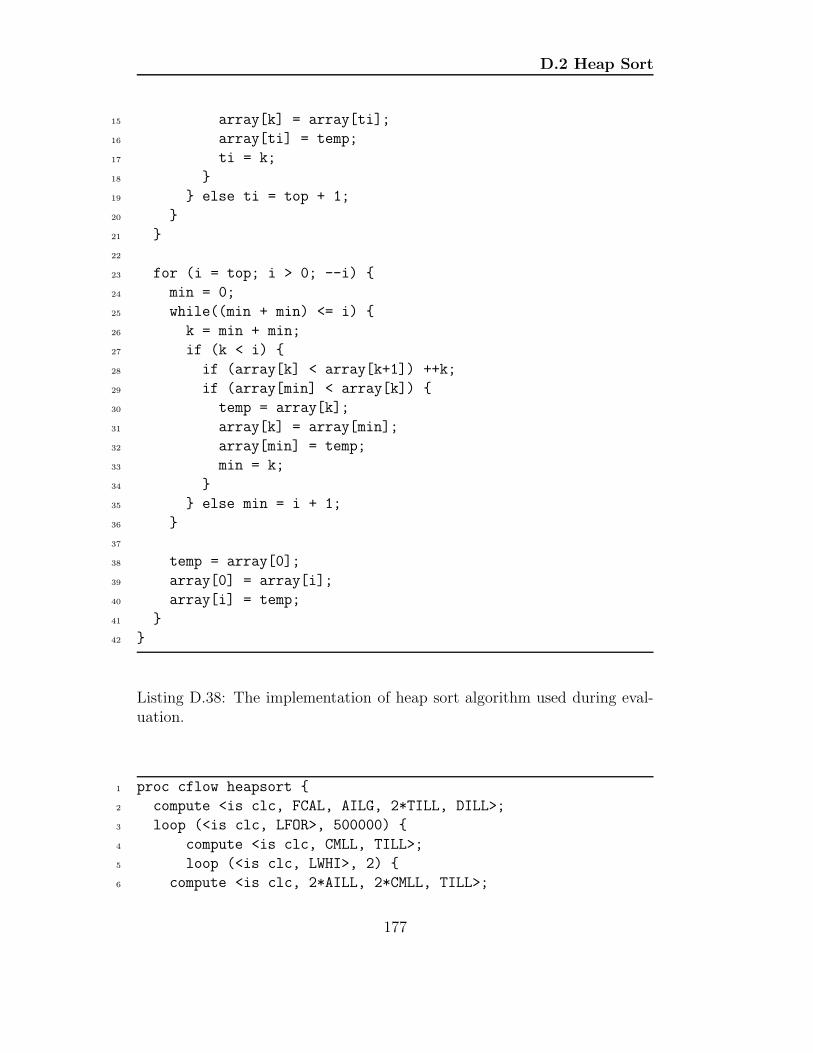
D.2 Heap Sort
15 array[k] = array[ti];
16 array[ti] = temp;
17 ti = k;
18 }
19 } else ti = top + 1;
20 }
21 }
22
23 for (i = top; i > 0; --i) {
24 min = 0;
25 while((min + min) <= i) {
26 k = min + min;
27 if (k < i) {
28 if (array[k] < array[k+1]) ++k;
29 if (array[min] < array[k]) {
30 temp = array[k];
31 array[k] = array[min];
32 array[min] = temp;
33 min = k;
34 }
35 } else min = i + 1;
36 }
37
38 temp = array[0];
39 array[0] = array[i];
40 array[i] = temp;
41 }
42 }
Listing D.38: The implementation of heap sort algorithm used during eval-uation.
1 proc cflow heapsort {
2 compute <is clc, FCAL, AILG, 2*TILL, DILL>;
3 loop (<is clc, LFOR>, 500000) {
4 compute <is clc, CMLL, TILL>;
5 loop (<is clc, LWHI>, 2) {
6 compute <is clc, 2*AILL, 2*CMLL, TILL>;
177

D.2 Heap Sort
7 case (<is clc, IFBR>) {
8 0.5:
9 compute <is clc, 2*ARL1, CMLG>;
10 case (<is clc, IFBR>) {
11 0.5:
12 compute <is clc, INLL>;
13 }
14 }
15 compute <is clc, 2*ARL1, CMLG>;
16 case (<is clc, IFBR>) {
17 0.5:
18 compute <is clc, 4*ARL1, 2*TILL, 2*TILG>;
19 1-(0.5):
20 compute <is clc, AILL, TILL>;
21 }
22 }
23 compute <is clc, INLL>;
24 }
25 compute <is clc, TILL>;
26 loop (<is clc, LFOR>, 999999) {
27 compute <is clc, CMLL, SILL>;
28 loop (<is clc, LWHI>, 18) {
29 compute <is clc, 2*AILL, 2*CMLL, TILL>;
30 case (<is clc, IFBR>) {
31 0.5:
32 compute <is clc, 2*ARL1, CMLG>;
33 case (<is clc, IFBR>) {
34 0.5:
35 compute <is clc, INLL>;
36 }
37 }
38 compute <is clc, 2*ARL1, CMLG>;
39 case (<is clc, IFBR>) {
40 0.5:
41 compute <is clc, 4*ARL1, 2*TILL, 2*TILG>;
42 1-(0.5):
43 compute <is clc, AILL, TILL>;
44 }
45 }
46 compute <is clc, 4*ARL1, TILL, 2*TILG, INLL>;
47 }
178

D.3 Fast Fourier Transform
48 }
Listing D.39: The characterised proc cflow definition of the implementationof heap sort algorithm shown in listing D.38 sorting an array of 1000000integer.
D.3 Fast Fourier Transform
The Fast Fourier Transform (FFT) is a discrete Fourier transform algorithm
which reduces the number of computations needed for N points from 2N2 to
2NlgN , where lg is the base-2 logarithm. If the function to be transformed
is not harmonically related to the sampling frequency, the response of an
FFT looks like a sampling function. Aliasing can be reduced by apodisation
using a tapering function. However, aliasing reduction is at the expense of
broadening the spectral response.
The particular implementation shown in listing D.40 which is used dur-
ing evaluation performs a one-dimensional forward transform of N complex
numbers. This kernel exercises complex arithmetic, shuffling, non-constant
memory references and trigonometric functions. This is a CPU intensive
benchmark working at the kernel level. Listing D.41 is the characterised proc
cflow definition of the implementation of Fast Fourier Transform shown in
listing D.40 performing one-dimensional forward transform of 2097152 com-
plex numbers
179

D.3 Fast Fourier Transform
1 #define PI 3.14159265358979323
2 static int data_length;
3 static double *data;
4 static double totali,total;
5 static void fft(){
6 int i, direction, n, logn, bit, dual, j, a, b, nn,k,ii,jj;
7 double w_real, w_imag, wd_real, wd_imag, s, s2, t, theta;
8 double tmp_real, tmp_imag, z1_real, z1_imag, norm;
9 int log = 0;
10
11 direction = -1;
12 n = data_length/2;
13 if (n == 1) return;
14 for(k=1; k < n; k *= 2, log++);
15 if (n != (1 << log)) printf("Data length %d is not a power of 2!\n",n);
16 logn = log;
17
18 nn=data_length/2;
19 for (i = 0, j=0; i < nn - 1; i++) {
20 ii = 2*i;
21 jj = 2*j;
22 k = nn / 2 ;
23 if (i < j) {
24 tmp_real = data[ii];
25 tmp_imag = data[ii+1];
26 data[ii] = data[jj];
27 data[ii+1] = data[jj+1];
28 data[jj] = tmp_real;
29 data[jj+1] = tmp_imag;
30 }
31 while (k <= j) {
32 j = j - k ;
33 k = k / 2 ;
34 }
35 j += k ;
36 }
37
38 for (bit = 0, dual = 1; bit < logn; bit++, dual *= 2) {
39 w_real = 1.0;
40 w_imag = 0.0;
41
180

D.3 Fast Fourier Transform
42 theta = 2.0 * direction * PI / (2.0 * (double) dual);
43 s = sin(theta);
44 t = sin(theta / 2.0);
45 s2 = 2.0 * t * t;
46
47 for (b = 0; b < n; b += 2 * dual) {
48 i = 2*b ;
49 j = 2*(b + dual);
50 wd_real = data[j] ;
51 wd_imag = data[j+1] ;
52 data[j] = data[i] - wd_real;
53 data[j+1] = data[i+1] - wd_imag;
54 data[i] += wd_real;
55 data[i+1]+= wd_imag;
56 }
57
58 for (a = 1; a < dual; a++) {
59 tmp_real = w_real - s * w_imag - s2 * w_real;
60 tmp_imag = w_imag + s * w_real - s2 * w_imag;
61 w_real = tmp_real;
62 w_imag = tmp_imag;
63
64 for (b = 0; b < n; b += 2 * dual) {
65 i = 2*(b + a);
66 j = 2*(b + a + dual);
67 z1_real = data[j];
68 z1_imag = data[j+1];
69 wd_real = w_real * z1_real - w_imag * z1_imag;
70 wd_imag = w_real * z1_imag + w_imag * z1_real;
71 data[j] = data[i] - wd_real;
72 data[j+1] = data[i+1] - wd_imag;
73 data[i] += wd_real;
74 data[i+1]+= wd_imag;
75 }
76 }
77 }
78
79 for (i=0; i<data_length; i++) {
80 total += data[i];
81 }
82
181

D.3 Fast Fourier Transform
83 direction = -1;
84 n = data_length/2;
85 if (n == 1) return;
86 for(k=1; k < n; k *= 2, log++);
87 if (n != (1 << log)) printf("Data length %d is not a power of 2!\n",n);
88 logn = log;
89
90 nn=data_length/2;
91 for (i = 0, j=0; i < nn - 1; i++) {
92 ii = 2*i;
93 jj = 2*j;
94 k = nn / 2 ;
95 if (i < j) {
96 tmp_real = data[ii];
97 tmp_imag = data[ii+1];
98 data[ii] = data[jj];
99 data[ii+1] = data[jj+1];
100 data[jj] = tmp_real;
101 data[jj+1] = tmp_imag;
102 }
103 while (k <= j) {
104 j = j - k ;
105 k = k / 2 ;
106 }
107 j += k ;
108 }
109
110 for (bit = 0, dual = 1; bit < logn; bit++, dual *= 2) {
111 w_real = 1.0;
112 w_imag = 0.0;
113 theta = 2.0 * direction * PI / (2.0 * (double) dual);
114 s = sin(theta);
115 t = sin(theta / 2.0);
116 s2 = 2.0 * t * t;
117 for (b = 0; b < n; b += 2 * dual) {
118 i = 2*b ;
119 j = 2*(b + dual);
120 wd_real = data[j] ;
121 wd_imag = data[j+1] ;
122 data[j] = data[i] - wd_real;
123 data[j+1] = data[i+1] - wd_imag;
182

D.3 Fast Fourier Transform
124 data[i] += wd_real;
125 data[i+1]+= wd_imag;
126 }
127 for (a = 1; a < dual; a++) {
128 tmp_real = w_real - s * w_imag - s2 * w_real;
129 tmp_imag = w_imag + s * w_real - s2 * w_imag;
130 w_real = tmp_real;
131 w_imag = tmp_imag;
132 for (b = 0; b < n; b += 2 * dual) {
133 i = 2*(b + a);
134 j = 2*(b + a + dual);
135 z1_real = data[j];
136 z1_imag = data[j+1];
137 wd_real = w_real * z1_real - w_imag * z1_imag;
138 wd_imag = w_real * z1_imag + w_imag * z1_real;
139 data[j] = data[i] - wd_real;
140 data[j+1] = data[i+1] - wd_imag;
141 data[i] += wd_real;
142 data[i+1]+= wd_imag;
143 }
144 }
145 }
146
147 n = data_length/2;
148 norm=1/((double) n);
149
150 for(i=0; i<data_length; i++)
151 data[i] *= norm;
152
153 for(i=0; i<data_length; i++) {
154 totali += data[i];
155 }
156 }
157
Listing D.40: The implementation of Fast Fourier Transform algorithm usedduring evaluation.
183

D.3 Fast Fourier Transform
1 proc cflow fft {
2 compute <is clc, FCAL, SILL, 2*TILL, DILG, CMLL>;
3 case (<is clc, IFBR>) {
4 0.1:
5 compute <is clc, BRTN>;
6 return;
7 }
8 compute <is clc, SILL>;
9 loop (<is clc, LFOR>, 21) {
10 compute <is clc, CMLL, MILL, SILL, INLL>;
11 }
12 compute <is clc, CMLL>;
13 case (<is clc, IFBR>) {
14 0.1:
15 call cflow printf;
16 }
17 compute <is clc, 2*TILL, DILG, 2*SILL>;
18 loop (<is clc, LFOR>, 2097151) {
19 compute <is clc, AILL, 2*CMLL, 2*MILL, 3*TILL, DILL>;
20 case (<is clc, IFBR>) {
21 0.5:
22 compute <is clc, 8*ARD1, 2*TFDL, 4*TFDG>;
23 }
24 loop (<is clc, LWHI>, 2) {
25 compute <is clc, CMLL, AILL, 2*TILL, DILL>;
26 }
27 compute <is clc, AILL, TILL, INLL>;
28 }
29 compute <is clc, 2*SILL>;
30 loop (<is clc, LFOR>, 21) {
31 compute <is clc, CMLL, 2*SFDL, 5*MFDL, 2*DFDL, 4*TFDL, 2*SIND, SILL
32 >;
33 loop (<is clc, LFOR>, 99864) {
34 compute <is clc, CMLL, 3*MILL, 3*TILL, 2*AILL, 8*ARD1, 2*TFDL
35 , 4*AFDG, 4*TFDG>;
36 }
37 compute <is clc, SILL>;
38 loop (<is clc, LFOR>, 104856) {
39 compute <is clc, CMLL, 4*MFDL, 4*AFDL, 4*TFDL, SILL>;
40 loop (<is clc, LFOR>, 10) {
41 compute <is clc, CMLL, 4*AILL, 3*MILL, 3*TILL, 8*ARD1
184

D.3 Fast Fourier Transform
42 , 4*TFDL, 4*MFDL, 2*AFDL, 4*AFDG, 4*TFDG>;
43 }
44 compute <is clc, INLL>;
45 }
46 compute <is clc, INLL, MILL, SILL>;
47 }
48 compute <is clc, SILL>;
49 loop (<is clc, LFOR>, 4194304) {
50 compute <is clc, CMLL, ARD1, AFDG, TFDG, INLL>;
51 }
52 compute <is clc, 2*TILL, DILG, CMLL>;
53 case (<is clc, IFBR>) {
54 0.1:
55 compute <is clc, BRTN>;
56 return;
57 }
58 compute <is clc, SILL>;
59 loop (<is clc, LFOR>, 21) {
60 compute <is clc, CMLL, MILL, SILL, INLL>;
61 }
62 compute <is clc, CMLL>;
63 case (<is clc, IFBR>) {
64 0.1:
65 call cflow printf;
66 }
67 compute <is clc, 2*TILL, DILG, 2*SILL>;
68 loop (<is clc, LFOR>, 2097151) {
69 compute <is clc, AILL, 2*CMLL, 2*MILL, 3*TILL, DILL>;
70 case (<is clc, IFBR>) {
71 0.5:
72 compute <is clc, 8*ARD1, 2*TFDL, 4*TFDG>;
73 }
74 loop (<is clc, LWHI>, 2) {
75 compute <is clc, CMLL, AILL, 2*TILL, DILL>;
76 }
77 compute <is clc, AILL, TILL, INLL>;
78 }
79 compute <is clc, 2*SILL>;
80 loop (<is clc, LFOR>, 21) {
81 compute <is clc, CMLL, 2*SFDL, 5*MFDL, 2*DFDL, 4*TFDL
82 , 2*SIND, SILL>;
185
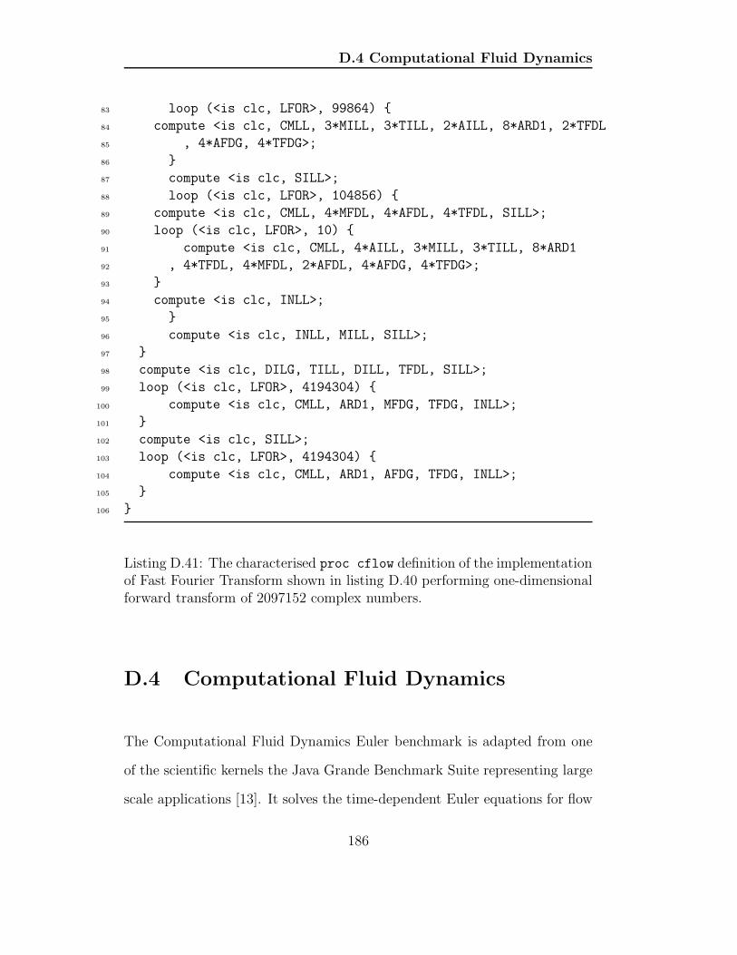
D.4 Computational Fluid Dynamics
83 loop (<is clc, LFOR>, 99864) {
84 compute <is clc, CMLL, 3*MILL, 3*TILL, 2*AILL, 8*ARD1, 2*TFDL
85 , 4*AFDG, 4*TFDG>;
86 }
87 compute <is clc, SILL>;
88 loop (<is clc, LFOR>, 104856) {
89 compute <is clc, CMLL, 4*MFDL, 4*AFDL, 4*TFDL, SILL>;
90 loop (<is clc, LFOR>, 10) {
91 compute <is clc, CMLL, 4*AILL, 3*MILL, 3*TILL, 8*ARD1
92 , 4*TFDL, 4*MFDL, 2*AFDL, 4*AFDG, 4*TFDG>;
93 }
94 compute <is clc, INLL>;
95 }
96 compute <is clc, INLL, MILL, SILL>;
97 }
98 compute <is clc, DILG, TILL, DILL, TFDL, SILL>;
99 loop (<is clc, LFOR>, 4194304) {
100 compute <is clc, CMLL, ARD1, MFDG, TFDG, INLL>;
101 }
102 compute <is clc, SILL>;
103 loop (<is clc, LFOR>, 4194304) {
104 compute <is clc, CMLL, ARD1, AFDG, TFDG, INLL>;
105 }
106 }
Listing D.41: The characterised proc cflow definition of the implementationof Fast Fourier Transform shown in listing D.40 performing one-dimensionalforward transform of 2097152 complex numbers.
D.4 Computational Fluid Dynamics
The Computational Fluid Dynamics Euler benchmark is adapted from one
of the scientific kernels the Java Grande Benchmark Suite representing large
scale applications [13]. It solves the time-dependent Euler equations for flow
186

D.4 Computational Fluid Dynamics
in a channel with a “bump” on one of the walls. A structured, irregular,
Nx4N mesh is employed, and the solution method is a finite volume scheme
using a fourth order Runge-Kutta method with both second and fourth order
damping. The solution is iterated for 200 timesteps. The C source code of
the implementation used for evaluation is around 2000 lines, therefore it is
not listed here.
187

Appendix E
cmodel - measured energy
consumption of individual clc
on workstation ip-115-69-dhcp
Table E.1 shows energy model cmodel containing the measured energy con-
sumption of individual clc executing on the workstation ip-115-69-dhcp.
Note due to the granularity of the measurements recorded by the digital mul-
timeter, some of the clc execution energy consumption cannot be recorded
while some of clc execution time cannot be obtained due to their insignifi-
cances in terms of execution performance.
188

Table E.1:
opcode time power energy overhead
SISL 0.000644827 35.37 2.280753099e-08 NULL
SISG 0.000638161 34.83 2.222714763e-08 NULL
SILL 0.000643161 35.54 2.285794194e-08 NULL
SILG 0.000649827 35.38 2.299087926e-08 NULL
SFSL 0.000608161 36.04 2.191812244e-08 NULL
SFSG 0.000634827 32.39 2.056204653e-08 NULL
SFDL 0.00120649 38.57 4.65343193e-08 NULL
SFDG 0.00125149 39.67 4.96466083e-08 NULL
SCHL 0.000634827 35.72 2.267602044e-08 NULL
SCHG 0.000634827 35.63 2.261888601e-08 NULL
TISL 0.0125282 35.72 4.47507304e-07 NULL
TISG 0.000654827 46.52 3.046255204e-08 NULL
TILL 0.000636494 35.71 2.272920074e-08 NULL
TILG 0.000634827 41.98 2.665003746e-08 NULL
TFSL 0.000634827 33.44 2.122861488e-08 NULL
TFSG 0.000636494 40.6 2.58416564e-08 NULL
TFDL 0.00127649 41.05 5.23999145e-08 NULL
TFDG 0.00125483 43.49 5.45725567e-08 NULL
TCHL 0.000983161 32.62 3.207071182e-08 NULL
TCHG 0.000658161 38.74 2.549715714e-08 NULL
Continued on next page
189

Table E.1 – continued from previous page
opcode time power energy overhead
AISL 0.0133633 0.04 5.34532e-10 SISL
AISG 0.000118333 0.02 2.36666e-12 SISG
AILL 9.5e-05 0.01 9.5e-13 SILL
AILG 9e-05 3.09 2.781e-10 SILG
AFSL 0.000241321 0.03 7.23963e-12 SFSL
AFSG 0.000204655 0.0 0.0 SFSG
AFDL 0.0 38.64 0.0 SFDL
AFDG 0.0 24.54 0.0 SFDG
ACHL 0.000118333 0.02 2.36666e-12 SCHL
ACHG 0.00011 0.02 2.2e-12 SCHG
INSL 0.00190965 0.03 5.72895e-11 SISL
INSG 0.00189632 0.03 5.68896e-11 SISG
INLL 0.00146132 0.03 4.38396e-11 SILL
INLG 0.00151465 0.03 4.54395e-11 SILG
MISL 0.0208997 0.04 8.35988e-10 SISL
MISG 0.00500632 0.03 1.501896e-10 SISG
MILL 0.000676321 0.02 1.352642e-11 SILL
MILG 0.00113465 0.02 2.2693e-11 SILG
MFSL 0.000256321 0.02 5.12642e-12 SFSL
MFSG 0.000264655 14.9 3.9433595e-09 SFSG
MFDL 0.0 32.47 0.0 SFDL
Continued on next page
190

Table E.1 – continued from previous page
opcode time power energy overhead
MFDG 0.0 41.86 0.0 SFDG
MCHL 0.00498465 0.02 9.9693e-11 SCHL
MCHG 0.00499465 0.03 1.498395e-10 SCHG
DISL 0.0119047 0.03 3.57141e-10 SISL
DISG 0.0123663 0.04 4.94652e-10 SISG
DILL 0.0153063 0.04 6.12252e-10 SILL
DILG 0.0206197 0.04 8.24788e-10 SILG
DFSL 0.0151163 0.03 4.53489e-10 SFSL
DFSG 0.0148647 0.02 2.97294e-10 SFSG
DFDL 0.014258 0.02 2.8516e-10 SFDL
DFDG 0.014213 0.02 2.8426e-10 SFDG
DCHL 0.0108097 0.02 2.16194e-10 SCHL
DCHG 0.0107697 0.04 4.30788e-10 SCHG
ISIL 0.000689482 40.16 2.768959712e-08 NULL
ISCH 0.0124245 4.02 4.994649e-08 NULL
ISFS 0.00219448 17.03 3.73719944e-08 NULL
ISFD 0.00221448 36.09 7.99205832e-08 NULL
ILIS 0.000659482 4.24 2.79620368e-09 NULL
ILCH 0.000654482 33.68 2.204295376e-08 NULL
ILFS 0.000879482 39.14 3.442292548e-08 NULL
ILFD 0.000829482 15.15 1.25666523e-08 NULL
Continued on next page
191

Table E.1 – continued from previous page
opcode time power energy overhead
FSCH 0.00740948 42.17 3.124577716e-07 NULL
FSIS 0.00658448 35.16 2.315103168e-07 NULL
FSIL 0.00655448 41.63 2.728630024e-07 NULL
FSFD 0.000719482 37.72 2.713886104e-08 NULL
FDCH 0.00737448 37.61 2.773541928e-07 NULL
FDIS 0.00657448 36.19 2.379304312e-07 NULL
FDIL 0.00652948 37.14 2.425048872e-07 NULL
FDFS 0.000709482 39.22 2.782588404e-08 NULL
CHIS 0.000739482 38.5 2.8470057e-08 NULL
CHIL 0.000659482 35.75 2.35764815e-08 NULL
CHFS 0.00364448 35.63 1.298528224e-07 NULL
CHFD 0.00364948 24.83 9.06165884e-08 NULL
ARCN 2.46547e-05 0.01 2.46547e-13 SCHL
ARC1 9.46547e-05 0.01 9.46547e-13 SCHL
ARC2 0.000994655 0.04 3.97862e-11 SCHL
ARC3 0.00131465 0.03 3.94395e-11 SCHL
ARSN 3.96547e-05 0.02 7.93094e-13 SISL
ARS1 8.96547e-05 12.54 1.124269938e-09 SISL
ARS2 0.000429655 15.04 6.4620112e-09 SISL
ARS3 0.000874655 0.03 2.623965e-11 SISL
ARLN 1.63213e-05 0.0 0.0 SILL
Continued on next page
192

Table E.1 – continued from previous page
opcode time power energy overhead
ARL1 8.63213e-05 32.67 2.820116871e-09 SILL
ARL2 0.000451321 17.76 8.01546096e-09 SILL
ARL3 0.000876321 0.03 2.628963e-11 SILL
ARFN 0.0 0.02 0.0 SFSL
ARF1 0.000136321 16.96 2.31200416e-09 SFSL
ARF2 0.000516321 8.47 4.37323887e-09 SFSL
ARF3 0.000851321 0.03 2.553963e-11 SFSL
ARDN 8.7988e-05 29.69 2.61236372e-09 SFDL
ARD1 0.000212988 0.0 0.0 SFDL
ARD2 0.000602988 0.01 6.02988e-12 SFDL
ARD3 0.00131799 0.02 2.63598e-11 SFDL
POC1 0.000184655 0.0 0.0 SCHL
POC2 0.000489655 0.03 1.468965e-11 SCHL
POCA 0.000814655 0.02 1.62931e-11 SCHL
POS1 8.46547e-05 0.01 8.46547e-13 SISL
POS2 0.000454655 0.01 4.54655e-12 SISL
POSA 0.000809655 0.03 2.428965e-11 SISL
POL1 8.13213e-05 0.01 8.13213e-13 SILL
POL2 0.000461321 8.97 4.13804937e-09 SILL
POLA 0.000811321 0.02 1.622642e-11 SILL
POF1 0.000131321 0.01 1.31321e-12 SFSL
Continued on next page
193

Table E.1 – continued from previous page
opcode time power energy overhead
POF2 0.000751321 0.02 1.502642e-11 SFSL
POFA 0.000836321 0.02 1.672642e-11 SFSL
POD1 0.000212988 0.02 4.25976e-12 SFDL
POD2 0.000292988 0.01 2.92988e-12 SFDL
PODA 0.000842988 0.02 1.685976e-11 SFDL
ANDL 0.000941321 0.02 1.882642e-11 SILL
ANDG 0.000851321 0.03 2.553963e-11 SILL
CMLL 0.000306321 0.02 6.12642e-12 SILL
CMLG 0.000366321 0.01 3.66321e-12 SILL
CMSL 0.00243632 0.04 9.74528e-11 SILL
CMSG 0.00312132 0.03 9.36396e-11 SILL
CMCL 0.00223632 0.03 6.70896e-11 SILL
CMCG 0.00217132 0.03 6.51396e-11 SILL
CMFL 0.00260132 0.03 7.80396e-11 SILL
CMFG 0.00259132 0.03 7.77396e-11 SILL
CMDL 0.00253132 0.03 7.59396e-11 SILL
CMDG 0.00257632 0.03 7.72896e-11 SILL
IFBR 0.0 0.0 0.0 TILL
SWCL 4.9482e-05 36.7 1.8159894e-09 NULL
SWCG 4.482e-06 15 6.723e-11 NULL
SWSL 1.9482e-05 10.34 2.0144388e-10 NULL
Continued on next page
194

Table E.1 – continued from previous page
opcode time power energy overhead
SWSG 4.482e-06 17.26 7.735932e-11 NULL
SWLL 3.9482e-05 10.25 4.046905e-10 NULL
SWLG 1.9482e-05 10.54 2.0534028e-10 NULL
CACL 0.0 0.03 0.0 SWCL
CACG 1e-05 0.01 1e-13 SWCG
CASL 2.5e-05 29.88 7.47e-10 SWSL
CASG 2.0328e-21 0.02 4.0656e-29 SWSG
CALL 0.0 0.0 0.0 SWLL
CALG 0.0 0.01 0.0 SWLG
LTLL 0.000356321 0.01 3.56321e-12 SILL
LTLG 0.000479655 0.03 1.438965e-11 SILG
LELL 0.000386321 0.02 7.72642e-12 SILL
LELG 0.000454655 0.03 1.363965e-11 SILG
CELL 0.000356321 0.03 1.068963e-11 SILL
CELG 0.00130965 0.0 0.0 SILG
BALL 0.000116321 0.01 1.16321e-12 SILL
BALG 8.96547e-05 14.19 1.272200193e-09 SILG
BACL 0.000109655 6.52 7.149506e-10 SCHL
BACG 0.000129655 0.02 2.5931e-12 SCHG
BASL 0.0137597 0.02 2.75194e-10 SISL
BASG 0.000116321 0.01 1.16321e-12 SISG
Continued on next page
195

Table E.1 – continued from previous page
opcode time power energy overhead
FCAL 0.00428448 32.59 1.396312032e-07 NULL
FARC 7e-05 0.01 7e-13 FCAL
FARS 2.5e-05 0.01 2.5e-13 FCAL
FARL 0.0001 0.01 1e-12 FCAL
FARF 5.5e-05 0.01 5.5e-13 FCAL
FARD 0.00013 0.01 1.3e-12 FCAL
BGOT 2.4482e-05 46.47 1.13767854e-09 NULL
BCON 3.9482e-05 10.41 4.1100762e-10 NULL
BBRK 1.4482e-05 17.06 2.4706292e-10 NULL
BRTN 7.5e-05 15.18 1.1385e-09 FCAL
LWHI 9.482e-06 38.64 3.6638448e-10 NULL
LFOR 9.482e-06 15.69 1.4877258e-10 NULL
LDWH 9.482e-06 32.85 3.114837e-10 NULL
LOGD 0.0974545 32.56 3.17311852e-06 NULL
EXPD 0.111945 34.34 3.8441913e-06 NULL
SQRD 0.0411445 32.44 1.33472758e-06 NULL
SIND 1.4482e-05 38.79 5.6175678e-10 NULL
TAND 4.4482e-05 33 1.467906e-09 NULL
ABSD 2.6494e-05 16.63 4.4059522e-10 NULL
ABSI 1.6494e-05 22.58 3.7243452e-10 NULL
ABSL 1.98273e-05 24.26 4.81010298e-10 NULL
Continued on next page
196

Table E.1 – continued from previous page
opcode time power energy overhead
MODD 0.0610595 40.06 2.44604357e-06 NULL
POWD 0.237224 31.52 7.47730048e-06 NULL
197

Bibliography
[1] Nevine AbouGhazaleh, Bruce Childers, Daniel Mosse, Rami Melhem,
and Matthew Craven. Energy management for real-time embedded ap-
plications with compiler support. In LCTES ’03: Proceedings of the
2003 ACM SIGPLAN conference on Language, compiler, and tool for
embedded systems, pages 284–293, New York, NY, USA, 2003. ACM
Press.
[2] ACPI Overview.
http://www.acpi.info/presentations/ACPI Overview.pdf.
[3] Advanced Configuration and Power Interface Specification, 2.0c edition,
August 2003.
[4] Cliff Addison, James Allwright, Norman Binsted, Nigel Bishop, Bryan
Carpenter, Peter Dalloz, David Gee, Vladimir Getov, Tony Hey, Roger
Hockney, Max Lemke, John Merlin, Mark Pinches, Chris Scott, and
Ivan Wolton. The Genesis distributed-memory benchmarks. Part 1:
Methodology and general relativity benchmark with results for the
198

BIBLIOGRAPHY
SUPRENUM computer. Concurrency: Practice and Experience,
5(1):1–22, 1993.
[5] Computer industry almanac. available in
http://www.c-i-a.com/pr1002.htm.
[6] N. An, S. Gurumurthi, A. Sivasubramaniam, N. Vijaykrishnan, Kan-
demir M., and M. J. Irwin. Energy-performance trade-offs for spatial ac-
cess methods on memory-resident data. The VLDB Journal, 11(3):179–
197, November 2002.
[7] David F. Bacon, Susan L. Graham, and Oliver J. Sharp. Compiler trans-
formations for high-performance computing. ACM Computing Surveys,
26(4):345–420, December 1994.
[8] D. Bailey, E. Barszez, L. Dagum, and H. Simon. Nas parallel benchmark
results. Supercomputing, pages 368–393, 1992.
[9] Luca Benini and Giovanni de Micheli. System-level power optimiza-
tion: techniques and tools. ACM Trans. Des. Autom. Electron. Syst.,
5(2):115–192, April 2000.
[10] H. Blanchard, B. Brock, M. Locke, M. Orvek, R. Paulsen, and K. Ra-
jamani. Dynamic power management for embedded systems. IBM and
MontaVista Software Version 1.1 Whitepaper, November 2002.
[11] Barry B. Brey. The Intel Microprocessors: 8086/8088, 80286, 80386,
80486, Pentium, Pentium Pro, and Pentium II Processors : architec-
ture, programming, and interfacing. Prentice Hall Inc, 5th edition, 2000.
199

BIBLIOGRAPHY
[12] J. M. Bull, L. A. Smith, L. Pottage, and R. Freeman. Benchmarking
java against c and fortran for scientific applications. In Java Grande,
pages 97–105, 2001.
[13] J. M. Bull, L. A. Smith, M. D. Westhead, D. S. Henty, and R. A. Davey.
A benchmark suite for high performance Java. Concurrency: Practice
and Experience, 12(6):375–388, 2000.
[14] Junwei Cao, Darren J. Kerbyson, Efstathios Papaefstathiou, and Gra-
ham R. Nudd. Performance modelling of parallel and distributed com-
puting using pace. IEEE International Performance Computing and
Communications Conference, IPCCC-2000, pages 485–492, February
2000.
[15] Cell phone growth projected.
http://sanjose.bizjournals.com/sanjose/stories/2001/08/06/.
[16] A.T.S. Chan, Peter Y.H. Wong, and S.N. Chuang. Crl: A context-aware
request language for mobile computing. In Jiannong Cao, Laurence T.
Yang, Minyi Guo, and et al., editors, Second International Symposium
on Parallel and Distributed Processing and Applications (ISPA’04), vol-
ume 3358, page 529, December 2004.
[17] A. Chandrakasan and R. Brodersen. Low Power Digital CMOS Design.
Kluwer Academic Publishers, 1995.
[18] Eui-Young Chung, Luca Benini, and Giovanni De Micheli. Source code
transformation based on software cost analysis. In ISSS ’01: Proceedings
200

BIBLIOGRAPHY
of the 14th international symposium on Systems synthesis, pages 153–
158, New York, NY, USA, 2001. ACM Press.
[19] Common format and mime type for csv files.
http://www.shaftek.org/publications.shtml.
[20] P.J. de Langen and B.H.H. Juurlink. Reducing conflict misses in caches.
In Proceedings of the 14th Annual Workshop on Circuits, Systems and
Signal Processing, ProRisc 2003, pages 505–510, November 2003.
[21] K. Dixit. The spec benchmarks. Computer Benchmarks, pages 149–163,
1993.
[22] J. J. Dongarra. Performance of various computers using standard linear
equations software in a Fortran environment. In Walter J. Karplus,
editor, Multiprocessors and array processors: proceedings of the Third
Conference on Multiprocessors and Array Processors: 14–16 January
1987, San Diego, California, pages 15–32, San Diego, CA, USA, 1987.
Society for Computer Simulation.
[23] Jack J. Dongarra. Performance of various computers using standard
linear equations software. Technical report, Knoxville, TN, USA, 1989.
[24] Fred Douglis, P. Krishnan, and Brian Marsh. Thwarting the power-
hungry disk. In USENIX Winter, pages 292–306, January 1994.
[25] J. Eagan, M. J. Harrold, J. Jones, and J. Stasko. Vi-
sually encoding program test information to find faults
201

BIBLIOGRAPHY
in software. Technical report, Atlanta, GA, June 2001.
http://www.cc.gatech.edu/aristotle/Tools/tarantula/.
[26] Stephen G. Eick and Joseph L. Steffen. Visualizing code profiling line
oriented statistics. In VIS ’92: Proceedings of the 3rd conference on
Visualization ’92, pages 210–217, Los Alamitos, CA, USA, 1992. IEEE
Computer Society Press.
[27] Stephen G. Eick, Joseph L. Steffen, and Jr. Eric E. Sumner. Seesoft-a
tool for visualizing line oriented software statistics. IEEE Trans. Softw.
Eng., 18(11):957–968, 1992.
[28] Shaun flisakowski’s site. http://www.spf-15.com/.
[29] B. P. Foley, P. J. Isitt, D. P. Spooner, S. A. Jarvis, and G. R. Nudd.
Implementing performance services in globus toolkit v3. In 20th Annual
UK Performance Engineering Workshop (UKPEW’ 2004), University
of Bradford, July 2004.
[30] I. Foster and C. Kesselman. The GRID: Blueprint for a New Computing
Infrastructure. Morgan-Kaufmann, 1998.
[31] S. Gurumurthi, A. Sivasubramaniam, M. Kandemir, and H. Franke.
Dynamic speed control for server class disks. Technical report, 2003.
CSE-03-007.
[32] S. Gurumurthi, A. Sivasubramaniam, M. Kandemir, and H. Franke. Re-
ducing disk power consumption in servers with drpm. IEEE Computer,
35(12):59–66, December 2003.
202

BIBLIOGRAPHY
[33] J. Harper, D. Kerbyson, and Graham Nudd. Analytical modeling of
set-associative cache behaviour. IEEE Transactions on Computers,
49(10):1009–1024, October 1999.
[34] R. Hockney and M. Berry. Parkbench report: Public international
benchmarks for parallel computers. Scientific Programming, 3(2):101–
146, 1994.
[35] High performance systems research group.
http://www.dcs.warwick.ac.uk/research/hpsg.
[36] HPSG. PACE Reference Manual, 1999.
http://www.dcs.warwick.ac.uk/research/hpsg.
[37] Intel Corp. i486 Microprocessor, Hardware Reference Manual, 1990.
[38] Intel Corporation/Microsoft Corporation. APM Specification, 1st edi-
tion.
[39] R. Jain. The Art of Computer Performance Analysis. John Wiley and
Sons, 1991.
[40] Jeff Janzen. Calculating memory system power for
DDR SDRAM. Designline, 10(2), 2001. available at
http://download.micron.com/pdf/pubs/designline/dl201.pdf.
[41] Chandra Krintz, Ye Wen, and Rich Wolski. Application-level prediction
of battery dissipation. In ISLPED ’04: Proceedings of the 2004 interna-
tional symposium on Low power electronics and design, pages 224–229,
New York, NY, USA, 2004. ACM Press.
203

BIBLIOGRAPHY
[42] Monica D. Lam, Edward E. Rothberg, and Michael E. Wolf. The cache
performance and optimizations of blocked algorithms. In ASPLOS-IV:
Proceedings of the fourth international conference on Architectural sup-
port for programming languages and operating systems, pages 63–74,
New York, NY, USA, 1991. ACM Press.
[43] W. Leinberger and V. Kumar. Information power grid: The new frontier
in parallel computing? IEEE Concurrency, 7(4), 1999.
[44] Jonathan I. Maletic, Andrian Marcus, and Louis Feng. Source viewer 3d
(sv3d): a framework for software visualization. In ICSE’03: Proceedings
of the 25th International Conference on Software Engineering, pages
812–813, Washington, DC, USA, 2003. IEEE Computer Society.
[45] D. Marculescu. On the use of microarchitecture-driven dynamic voltage
scaling. In Workshop on Complexity-Effective Design, June 2000.
[46] A. Marcus, L. Feng, and J. I. Maletic. 3d representations for software
visualization. In SoftVis’03: Proceedings of the ACM Symposium on
Software Visualization, pages 27–36, San Diego, CA, June 2003.
[47] Gmc instruments group, gossen metrawatt, camille bauer.
http://www.gmc-instruments.de/.
[48] M.T.Heath and J.E.Finger. Paragraph: A performance vi-
sualization tool for mpi. Technical report, August 2003.
http://www.csar.uiuc.edu/software/paragraph.
204

BIBLIOGRAPHY
[49] T. Mudge. Power: A first-class design constraint. IEEE Computer,
34(4):52–57, April 2001.
[50] F. Najm. A survey of power estimation techniques in vlsi circuits. IEEE
Transactions on VLSI Systems, 2(4):446–455, December 1994.
[51] Graham R. Nudd, Darren J. Kerbyson, Efstathios Papaefstathiou,
John S. Harper, Stewart C. Perry, and Daniel V. Wilcox. PACE: A
toolset for the performance prediction of parallel and distributed sys-
tems. The International Journal of High Performance Computing Ap-
plications, 14(3):228–251, 2000.
[52] E. Papaefstathiou, D.J. Kerbyson, G.R. Nudd, and T.J. Atherton. An
overview of the chip3s performance prediction toolset for parallel sys-
tems. 8th ISCA International Conference on Parallel and Distributed
Computing Systems, pages 527–533, 1995.
[53] Efstathios Papaefstathiou. A Framework for Characterising Parallel
Systems for Performance Evaluation. PhD thesis, University of War-
wick, September 1995.
[54] Athanasios E. Papathanasiou and Michael L. Scott. Energy efficient
prefetching and caching. In Proceedings of the USENIX 2004 Annual
Technical Conference, June 2004.
[55] T. Pering, T. Burd, and R. Brodersen. Dynamic voltage scaling and
the design of a low-power microprocessor system. In Power Driven Mi-
croarchitecture Workshop, in conjunction with ISCA98, June 1998, June
1998.
205

BIBLIOGRAPHY
[56] A. Peymandoust, T. Simunic, and G. de Micheli. Low power embedded
software optimization using symbolic algebra. In DATE ’02: Proceedings
of the conference on Design, automation and test in Europe, pages 1052–
1057, Washington, DC, USA, 2002. IEEE Computer Society.
[57] A. Peymandoust, T. Simunic, and G. De Micheli. Lower power embed-
ded software optimization using symbolic algebra. IEEE Transactions on
Computer-Aided Design of Integrated Circuits and Systems, 22(8):964–
975, 2003. Special Issue of DAC 2002.
[58] Armita Peymandoust and Giovanni De Micheli. Symbolic algebra and
timing driven data-flow synthesis. In Proceedings of International Con-
ference on Computer Aided Design, pages 300–305, 2001.
[59] Power manager and acpi/apm for microsoft windows ce .net 4.2. avail-
able at http://msdn.microsoft.com.
[60] W.H. Press, S.A. Teukolsky, W.T. Vetterling, and B.P. Flannery. Nu-
merical Recipes in C: the art of scientific computing. Cambridge Uni-
versity Press, 2nd edition, 1992.
[61] F. Rawson. MEMPOWER: A Simple Memory Power Analysis Tool Set.
IBM Austin Research Laboratory, January 2004.
[62] Steven P. Reiss. Bee/hive: A software visualization back end. In Pro-
ceedings of ICSE 2001 Workshop on Software Visualization, pages 44–
48, Toronto, Ontario, Canada, 2001.
206

BIBLIOGRAPHY
[63] H. Saputra, M. Kandemir, N. Vijaykrishnan, M. J. Irwin, J. S. Hu, C-
H. Hsu, and U. Kremer. Energy-conscious compilation based on voltage
scaling. In LCTES/SCOPES ’02: Proceedings of the joint conference on
Languages, compilers and tools for embedded systems, pages 2–11, New
York, NY, USA, June 2002. ACM Press.
[64] Vivek Sarkar. Optimized unrolling of nested loops. In ICS ’00: Pro-
ceedings of the 14th international conference on Supercomputing, pages
153–166, New York, NY, USA, 2000. ACM Press.
[65] N. C. Shu. Visual Programming. Van Nostrand Reinhold Co, New York,
NY, USA, 1988.
[66] Tajana Simunic, Luca Benini, and Giovanni De Micheli. Cycle-accurate
simulation of energy consumption in embedded systems. In DAC
’99: Proceedings of the 36th Annual Conference on Design Automation
(DAC’99), pages 867–872, Washington, DC, USA, 1999. IEEE Com-
puter Society.
[67] Tajana Simunic, Giovanni de Micheli, Luca Benini, and Mat Hans.
Source code optimization and profiling of energy consumption in em-
bedded systems. In ISSS ’00: Proceedings of the 13th International
Symposium on System Synthesis (ISSS’00), pages 193–198, Washing-
ton, DC, USA, September 2000. IEEE Computer Society.
[68] D. Singh and V. Tiwari. Power challenges in the internet world. in
cool chips tutorial: An Industrial Perspective on Low Power Processor
207

BIBLIOGRAPHY
Design;. 32nd Annual International Symposium on Microarchitecture,
November 1999.
[69] John T. Stasko. The parade environment for visualizing parallel program
executions: A progress report. Technical report, Atlanta, GA, January
1995.
[70] V. Tiwari, S. Malik, and A. Wolfe. Power analysis of embedded software:
A first step towards software power minimization. IEEE Transactions
on VLSI Systems, 2(4), December 1994.
[71] V. Tiwari, S. Malik, A. Wolfe, and T.C. Lee. Instruction level power
analysis and optimization of software. Journal of VLSI Signal Processing
Systems, 13(2), August 1996.
[72] James D. Turner. A Dynamic Prediction and Monitoring Framework
for Distributed Applications. PhD thesis, University of Warwick, 2003.
[73] Peter Y.H. Wong. Bytecode monitoring of java programs. BSc Project
Report, University of Warwick, 2003.
[74] Qing Wu, Qinru Qiu, Massoud Pedram, and Chih-Shun Ding. Cycle-
accurate macro-models for rt-level power analysis. IEEE Transactions
on Very Large Scale Integration (VLSI) Systems, 6(4):520–528, 1998.
[75] Jianwen Zhu, Poonam Agrawal, and Daniel D. Gajski. Rt level power
analysis. In Proceeding of Asia and South Pacific Design Automation
Conference, February 1997.
208


