An introduction to the LMD Mars GCM The LMD Mars GCM team 15/10/2007.
70
An introduction to the LMD Mars GCM The LMD Mars GCM team 15/10/2007
-
Upload
dana-turner -
Category
Documents
-
view
221 -
download
2
Transcript of An introduction to the LMD Mars GCM The LMD Mars GCM team 15/10/2007.

An introduction to the LMD Mars GCM
The LMD Mars GCM team
15/10/2007

General Circulation Models/Global Climate models
GCMs
Numerical simulators of the Earth or Mars environment: designed to simulate the « entire reality »
Used on Earth for:
• Understanding the climate system: coupling with oceans, clouds, etc…
• Weather forecasts & Meteorological data assimilation• Climate changes, paleoclimates simulations• Chemistry, hydrology, biosphere studies, etc...
General Circulation Models/Global Climate models
GCMs
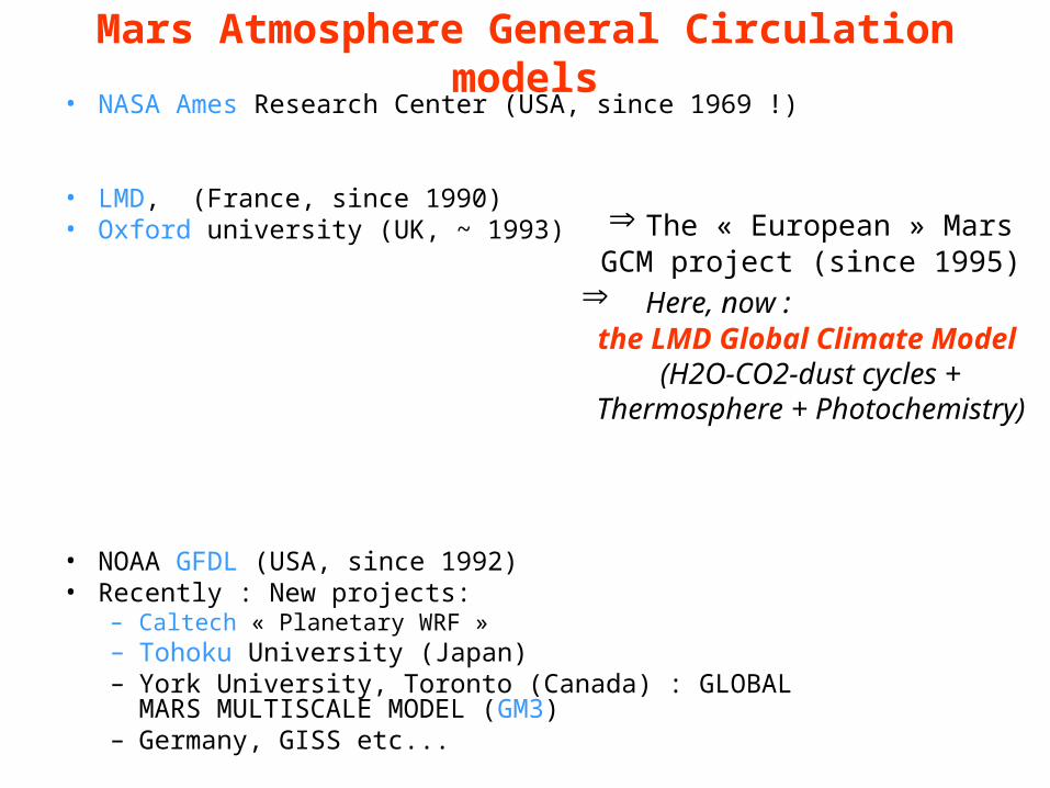
• NASA Ames Research Center (USA, since 1969 !)
• LMD, (France, since 1990)• Oxford university (UK, ~ 1993)
• NOAA GFDL (USA, since 1992) • Recently : New projects:
– Caltech « Planetary WRF » – Tohoku University (Japan)– York University, Toronto (Canada) : GLOBAL MARS
MULTISCALE MODEL (GM3) – Germany, GISS etc...
Mars Atmosphere General Circulation models
The « European » Mars GCM project (since 1995)
Here, now :the LMD Global Climate Model
(H2O-CO2-dust cycles + Thermosphere + Photochemistry)


The minimum General
Circulation Model for Mars1) Hydrodynamical code to compute large scale atmospheric
motions LMD : grid point model :
Typical resolution 64x48 , possibility of zoom
2) Physical parameterizations to force the dynamic to compute the details of the local
climate• Radiative heating & cooling of the atmosphere
(solar and thermal IR) by CO2 and dust• Surface thermal balance • Subgrid scale atmospheric motions :
Turbulence in the boundary layer Convection Relief drag Gravity wave drag
• CO2 condensation :
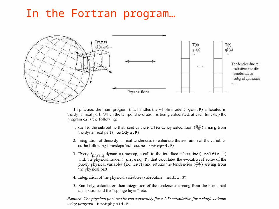
In the Fortran program…


The dynamical core
• Solve the Navier-Stokes equations simplified by the following assumption:– The atmosphere is thin compared to the planet radius – Hydrostatic approximation (the vertical wind is much smaller
than the horizontal one...)– Limited resolution : requires some “numerical dissipation” to
absorb the energy cascad toward small scale and stabilize the model create model dependent behavior...
• Horizontal discretization (~100-300 km):– Grid point models at LMD (and also at NASA Ames, GFDL,
WRF)– Exist also : Spectral models (in the Fourrier space) (Oxford,
Tokohu)
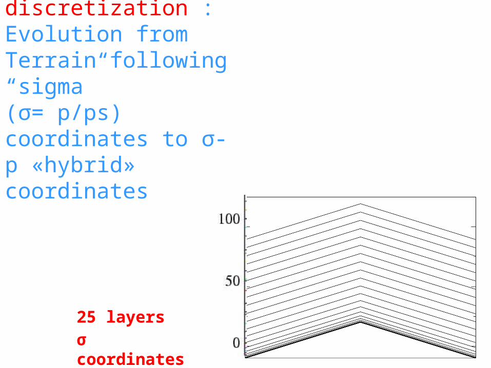
Vertical discretization : Evolution from Terrain following “sigma” (σ= p/ps) coordinates to σ-p «hybrid» coordinates
25 layersσ coordinates

32 layershybrid coordinates
Vertical discretization : Evolution from Terrain following “sigma” (σ= p/ps) coordinates to σ-p «hybrid» coordinates
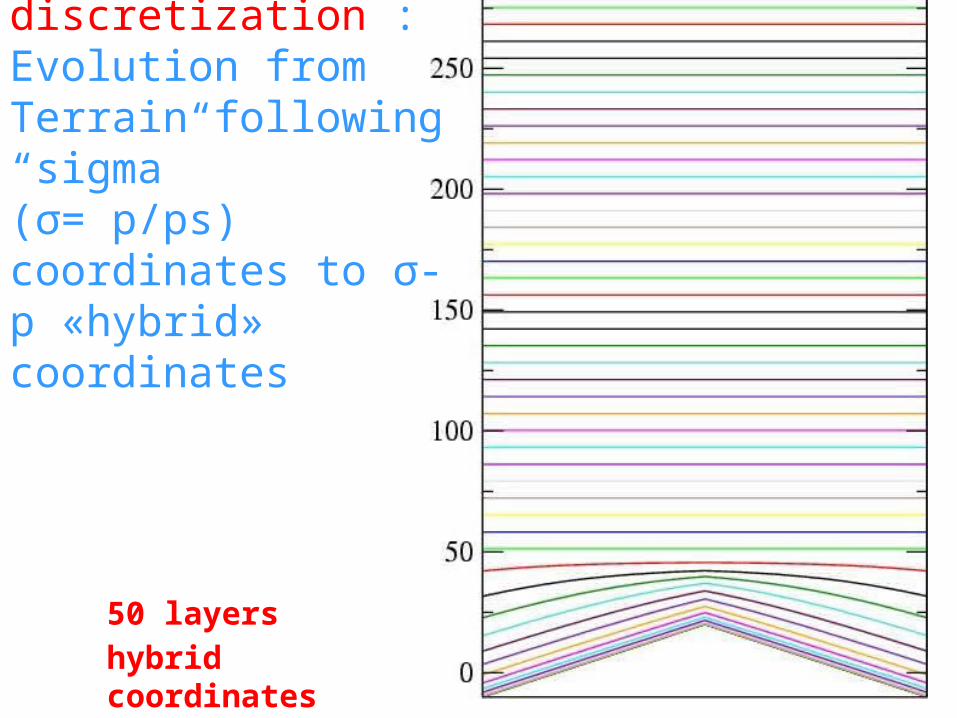
50 layershybrid coordinates
Vertical discretization : Evolution from Terrain following “sigma” (σ= p/ps) coordinates to σ-p «hybrid» coordinates

vertical grid
Numbers of layers depends of project :
• 50 layers : full model with Thermosphere (top above 300 km)
• 32 layers : top above 120 km (no thermosphere)
• 25 layer : reference for low atmosphere studies
• 18 layers : for long paleoclimate studies
Exemple : 32 layers

In the Fortran program…
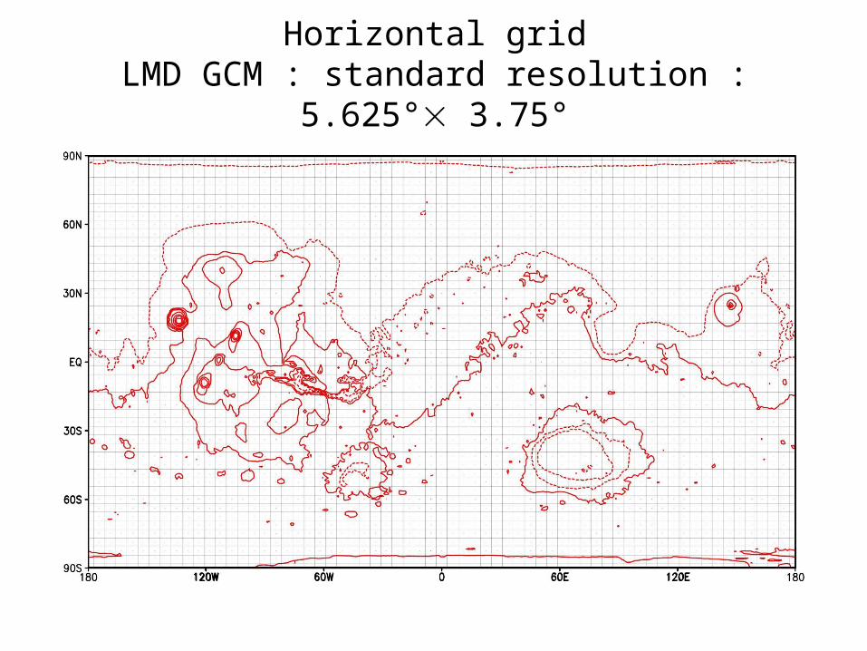
Horizontal gridLMD GCM : standard resolution : 5.625° 3.75°

LMD GCM : high resolution : 2° 2°

GCM : Zoomed grid to reach resolution: 1.8° 0.6°at reduced cost

An example of discretized horizontal grid, in the Fortran program…

The input maps and climatology
• In the GCM, everything is deduced from physical equations and physical constants except :– Topography map– Albedo map– Thermal inertia map– Dust 3D climatology

GCM surface fields• MOLA topography (of course)• ALBEDO (old map…):
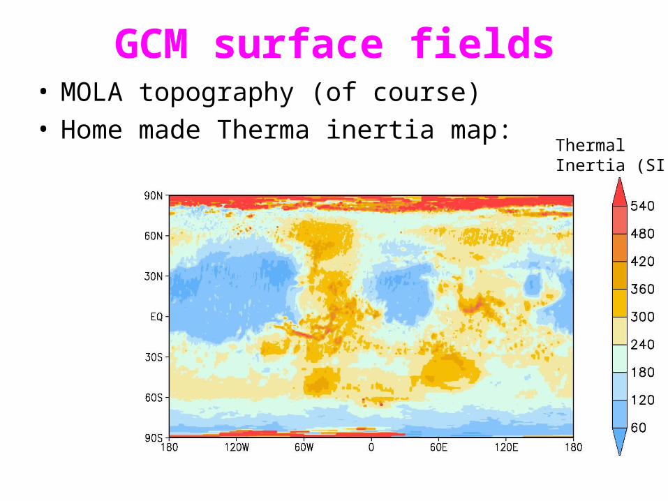
GCM surface fields• MOLA topography (of course)• Home made Therma inertia map:
ThermalInertia (SI)

GCM surface fields• MOLA topography (of course)• Home made Therma inertia map:
ThermalInertia (SI)
TES data :Mellon et al.(2000)

GCM surface fields• MOLA topography (of course)• Home made Therma inertia map:
ThermalInertia (SI)
Paige et al. (1994)Decrease : 25%
TES data :Mellon et al.(2000)
Palluconni and Kieffer (1981)Decrease : 8%
Paige and Keegan (1994)Decrease : 28%

DUST : so important for Atmospheric
dynamics and thermal structure • Problem : below 50 km :
the thermal structure is sensitive to the dust distribution
Require to prescribe a “dust distribution”problem analogous to Sea Surface Temperature forcing in Earth climate
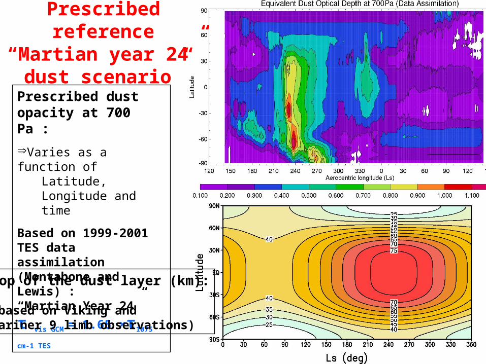
Prescribed reference “Martian year 24”
dust scenario”
Prescribed dust opacity at 700 Pa :
Varies as a function ofLatitude, Longitude and time
Based on 1999-2001 TES data assimilation (Montabone and Lewis) :“Martian Year 24”
τ vis GCM = 1.65 ×τ1075 cm-1 TES
Top of the dust layer (km):
(based on Viking andMariner 9 limb observations)
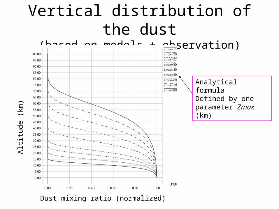
Vertical distribution of the dust(based on models + observation)
Alti
tude
(km
)
Dust mixing ratio (normalized)
Analytical formulaDefined by one parameter Zmax (km)

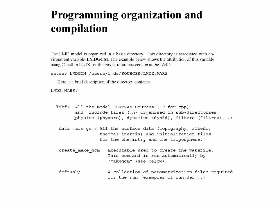
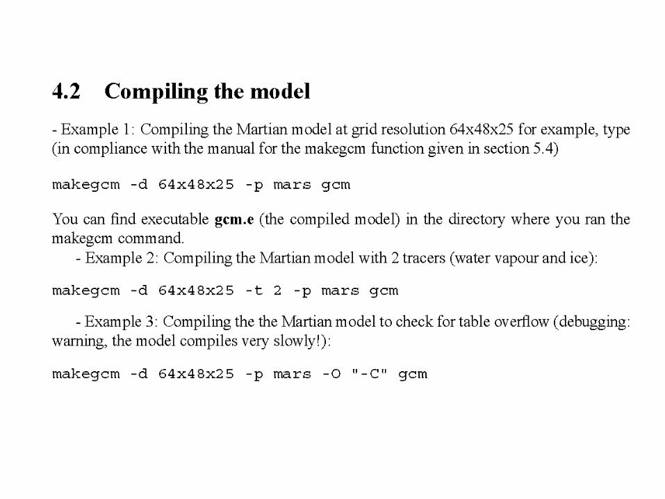
Some practical stuff
• The code is in Fortran (mostly Fortran 77, with some Fortran 90), compile on Unix/Linux platform (PC, SUN, DEC, etc…)
• It uses NetCDF library available on the web (http://www.unidata.ucar.edu/packages/netcdf/faq.html#howtoget)
• You put the source code somewhere, and run somewhere else
• For this purpose, one must initialize UNIX environment variable LMDGCM, LIBOGCM as well as NCDFINC and NCDFLIB (see User Manual)


Running the GCM:
•You need an initial state →
•You need some “definition” files :
•You can performed “chained simulations using various scripts (run0, run_mcd)…
To be detailed in practical work (see also the user manual)
• You get output files containing 4D data (3D+time) or 3D data (2D +time)
gcm
gcm

OUTPUT FILES
• NetCDF file diagfi.nc – NetCDF file diagfi.nc stores the instantaneous
physical variables throughout the sim ulation at regular intervals (set by the value of parameter ecritphy in parameter file “run.def”).
– Any variable from any sub-routine of the physical part can be stored by calling subroutine writediagfi
• NetCDF file stats.nc – Store a “mean” diurnal day, with timestep typically 2
martian hours.
How accurate are the temperature and wind
predictions ?

Surface temperatures

Mars Pathfinder data:Temperature at 1.2 m
MCD, Tsurf
MCD T(z=5m)
Obs (30 sols)

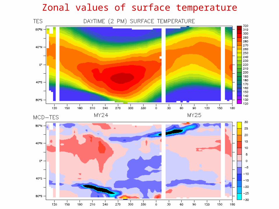
Zonal values of surface temperature
TES
Observation
GCM
Predictions
(retrieved through Mars
Climate Database
(“MCD”
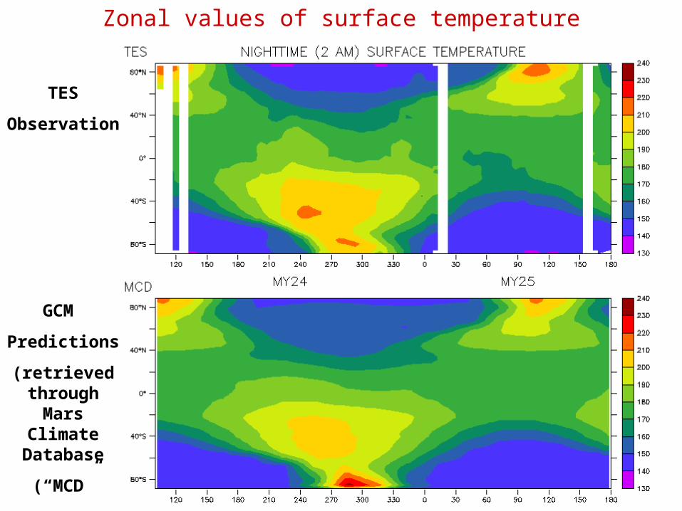
Zonal values of surface temperature
Zonal values of surface temperature
TES
Observation
GCM
Predictions
(retrieved through Mars
Climate Database
(“MCD”

Zonal values of surface temperature

• Statistics computed for:
MY24: 102.5 < Ls < 360
MY25: 0 < Ls < 180
-50 < latitude < 50
Bins of 1K
Distributions of surface temperature difference between MCDv4.2 and TES
Note: MEAN and RMS values are computed from histograms; blue curves are normal distributions of same MEAN and RMS
Atmospheric temperatures

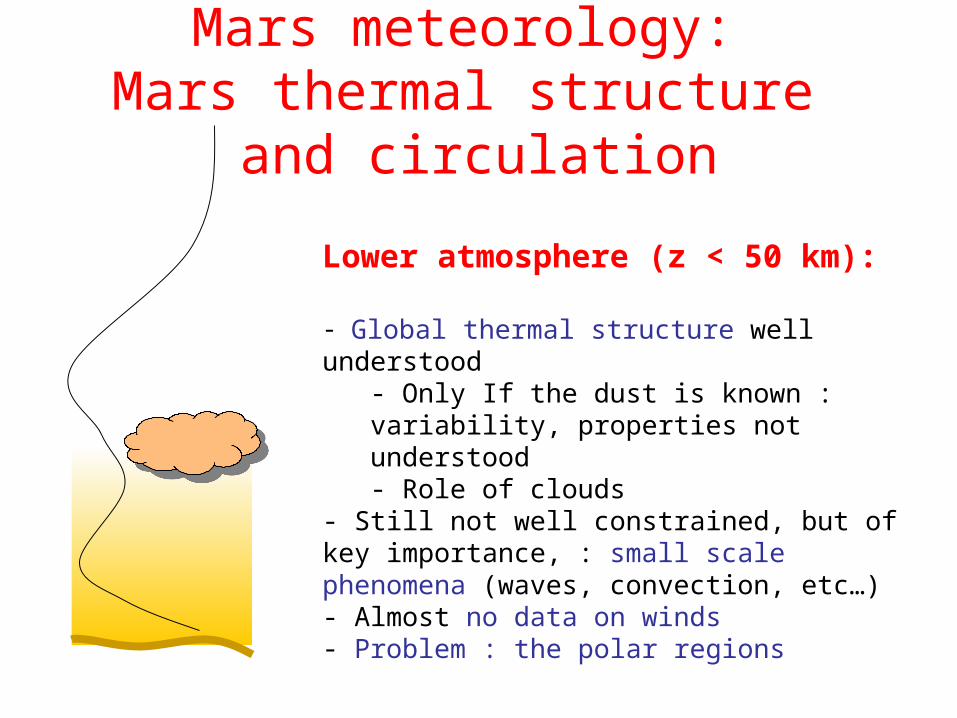
Mars meteorology: Mars thermal structure
and circulation
Lower atmosphere (z < 50 km): : - Global thermal structure: mostly well understood
If the dust is known : variability, properties not understood- Role of clouds :
- We can now study the details of meteorology (comparative meteorology)- Still not well constrained, but of key importance, :
-small scale Phenomena (waves, convection, etc…)
- Almost no data on winds- Big problem : the polar regions
TemperatureProfile

Comparison with MGS TES temperature observations
Zonal mean temperature (K)
GCM (« MCD V4.1 ») TES observations
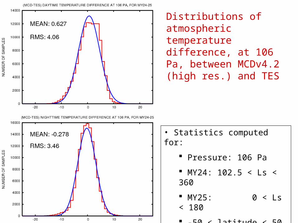
• Statistics computed for:
Pressure: 106 Pa
MY24: 102.5 < Ls < 360
MY25: 0 < Ls < 180
-50 < latitude < 50
Bins of 1K
Distributions of atmospheric temperature difference, at 106 Pa, between MCDv4.2 (high res.) and TES
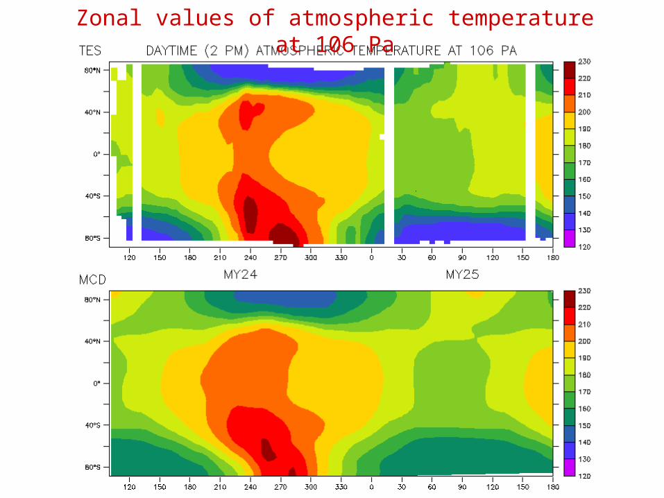
Zonal values of atmospheric temperature at 106 Pa
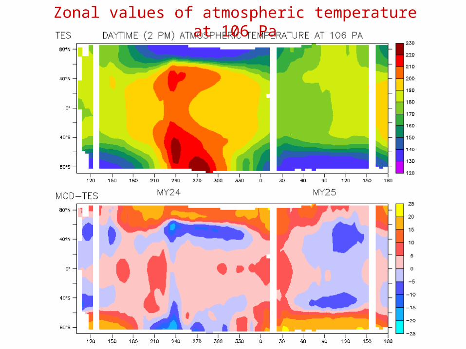
Zonal values of atmospheric temperature at 106 Pa
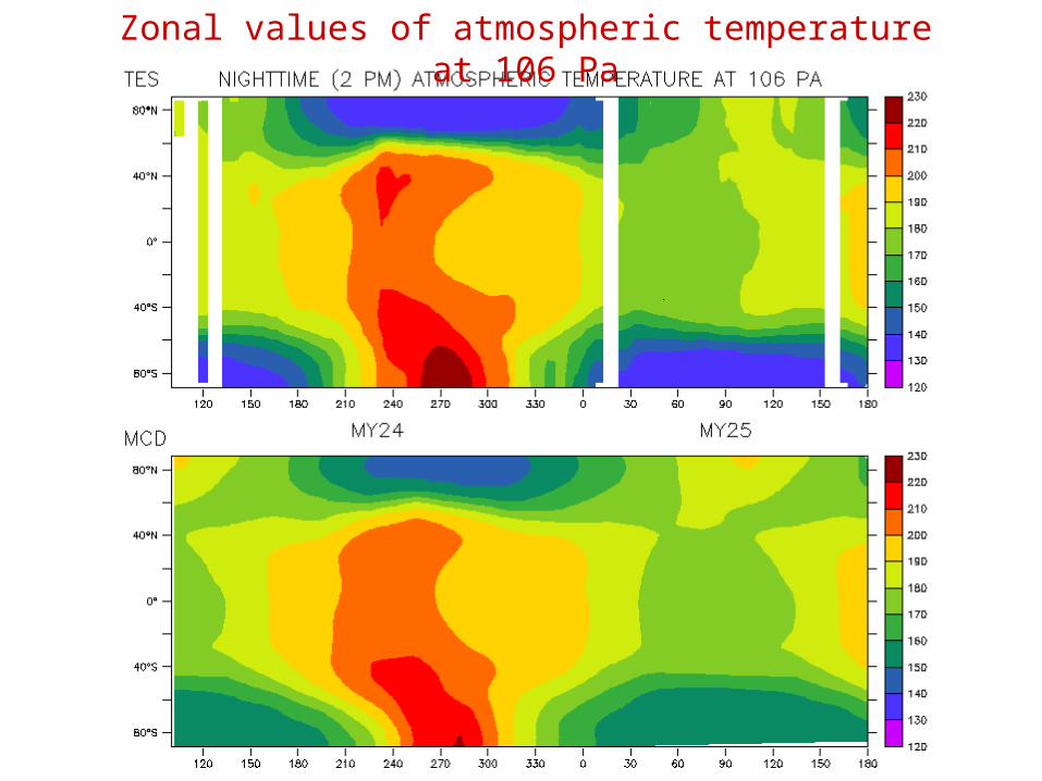
Zonal values of atmospheric temperature at 106 Pa

Zonal values of atmospheric temperature at 106 Pa

Comparison with MGS radio-occultation(In many cases, very good agreement)
At various seasons :
GCM
Observations

Comparison with MGS radio-occultation(In many cases, very good agreement)
At various local time
GCM
Observations

Comparison with MGS radio-occultationNorthern summer tropical inversions (1) CLOUDS !!
(radiatively active clouds will be included soon in the GCM)
GCM
Observations

Comparison with MGS radio-occultationMorning at high northern latitude in summer
radiative cooling to ice hazes ?
GCM
Observations

• Statistics computed for:
MY24 to MY27 (except MY25 storm)
-50 < latitude < 50
Bins of 1K
Altitude bands of 10 km
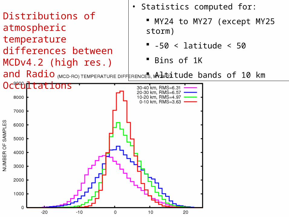
Distributions of atmospheric temperature differences between MCDv4.2 (high res.) and Radio Occultations

• Statistics computed for:
MY24 to MY27 (except MY25 storm)
-50 < latitude < 50
Bins of 1K
Altitude bands of 10 km
Distributions of atmospheric temperature differences between MCDv4.2 (high res.) and Radio Occultations
• Statistics computed for:
MY24 to MY27 (except MY25 storm)
-50 < latitude < 50
Bins of 1K
Altitude bands of 10 km
Distributions of atmospheric temperature differences between MCDv4.2 (high res.) and Radio Occultations
Mars meteorology: Mars thermal structure
and circulation
Lower atmosphere (z < 50 km): - Global thermal structure well understood
- Only If the dust is known : variability, properties not understood- Role of clouds
- Still not well constrained, but of key importance, : small scale phenomena (waves, convection, etc…)- Almost no data on winds- Problem : the polar regions

Comparison with MGS radio-occultationSouthern Winter polar night
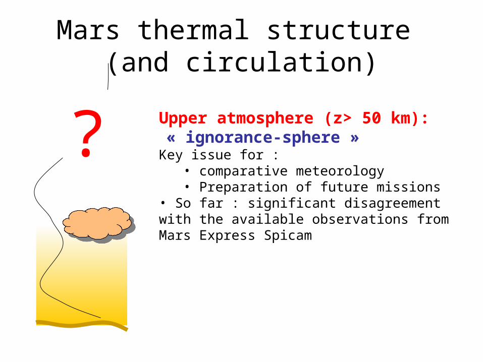
Mars thermal structure (and circulation)
Upper atmosphere (z> 50 km): « ignorance-sphere »Key issue for :
• comparative meteorology• Preparation of future missions
• So far : significant disagreement with the available observations from Mars Express Spicam
?
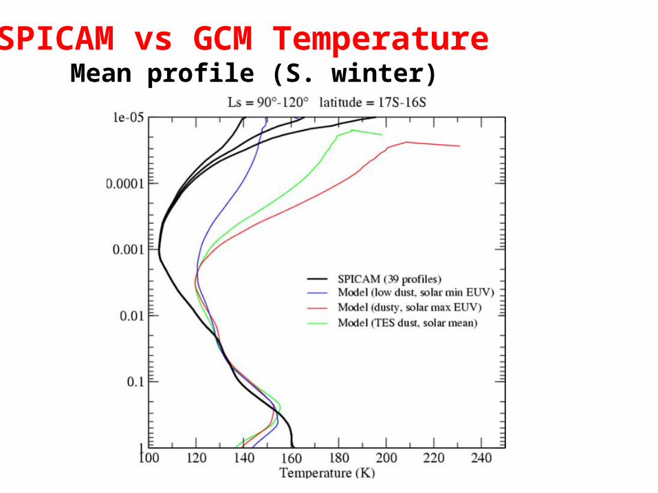
SPICAM vs GCM Temperature Mean profile (S. winter)
Using the GCM with tracers
• H2O + ice = water cycle
• Dust particles = dust cycle
• Chemical species = photochemistry and thermosphere

Modelling the CO2 cycle:
Modelling the dust cycle :
Modelling the water cycle:
Toward a “complete” model of the Martian climate system
Forget et al…
Newman et al.Forget et al…
Montmessin et al.Bottger et al.
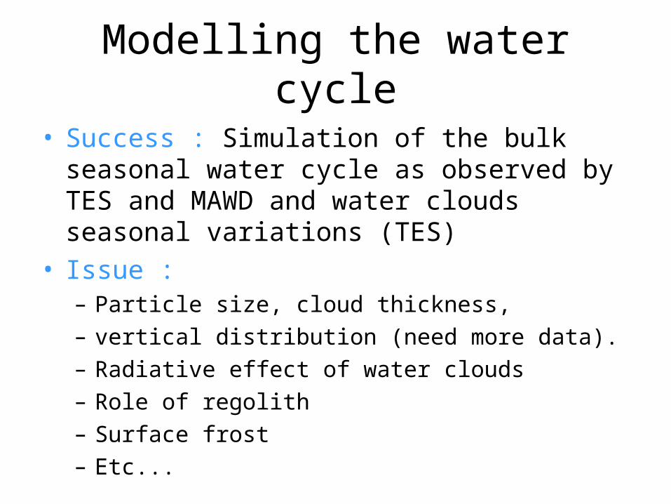
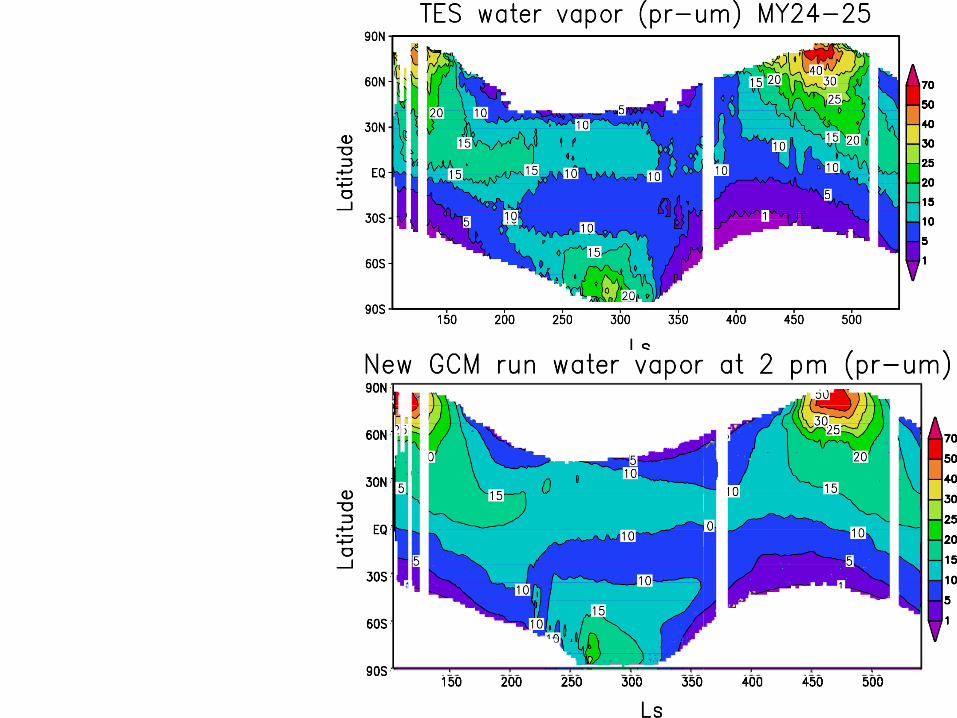
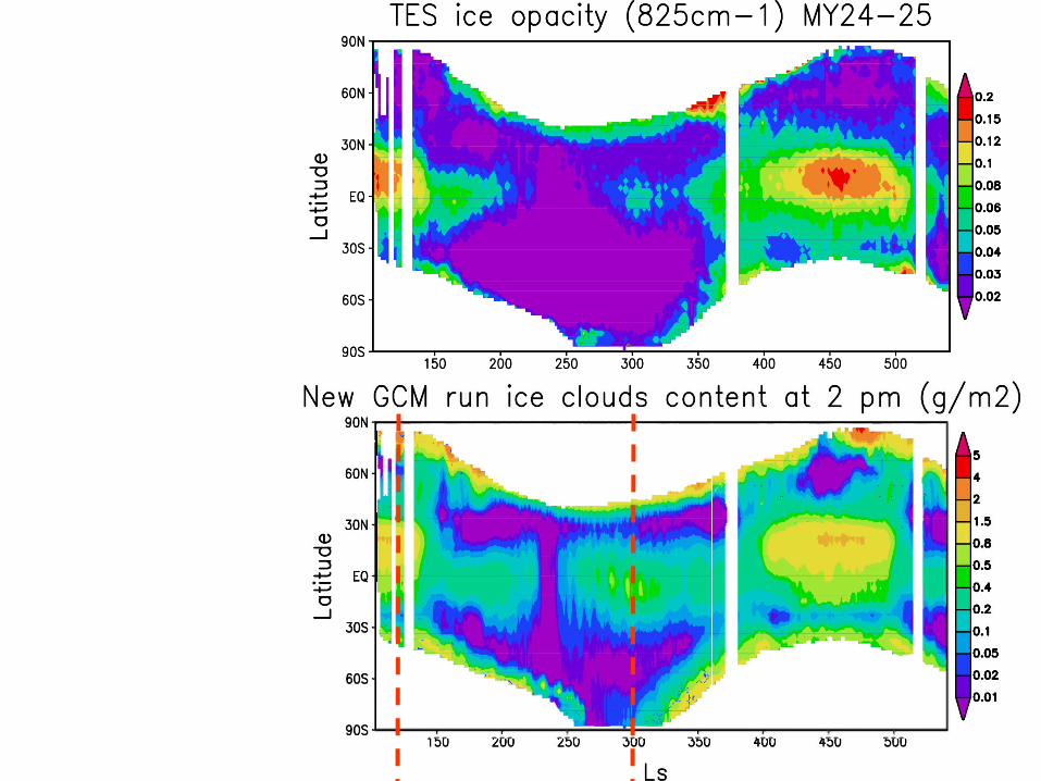
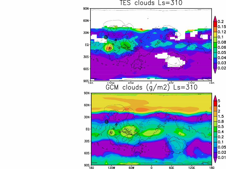
Modelling the water cycle
• Success : Simulation of the bulk seasonal water cycle as observed by TES and MAWD and water clouds seasonal variations (TES)
• Issue : – Particle size, cloud thickness, – vertical distribution (need more data).– Radiative effect of water clouds– Role of regolith– Surface frost– Etc...

Montmessin et al. 2004

Modelling the dust cycle
• Success : Simulation of local and regional dust storms. Initiate global dust storms.
Vertical and size distribution (need more data)
• Issue : Subgrid scale phenomenon
• Problem : The interranual variability
(Global dust storms...)

Dynamicwith
L. MontaboneM. Angelats
(LMD)
Dynamicwith
L. MontaboneM. Angelats
(LMD)
Thermosphere
Avec F. Gonzalez-G.(LMD),
M. Lopez V. (IAA) M. Angelats,
Thermosphere
Avec F. Gonzalez-G.(LMD),
M. Lopez V. (IAA) M. Angelats,
Photo-ChimistryF. Lefevre (SA)S. Lebonnois
(LMD)
Photo-ChimistryF. Lefevre (SA)S. Lebonnois
(LMD)
Water CycleF. Montmessin
(SA-LMD) H. Bottger (UO)
Water CycleF. Montmessin
(SA-LMD) H. Bottger (UO)
Dust Cycle
With Eric Hebrard(LISA)
C. Newman, (UO)
Dust Cycle
With Eric Hebrard(LISA)
C. Newman, (UO)
CO2 cycle
With E. Millour K. Dassas,G. Tobie,
(LMD)
CO2 cycle
With E. Millour K. Dassas,G. Tobie,
(LMD)
Mars GCM
Mars GCM
Synthesis : application of the LMD GCMStrong Collaboration with SA (IPSL, France),
University of Oxford (UK) , IAA (Grenade, Espagne)
Paléoclimate & Geologywith J.B. Madeleine (LMD)
B. Levrard, IMCCE)B; Haberle (NASA)
J. Head, YOU !
Paléoclimate & Geologywith J.B. Madeleine (LMD)
B. Levrard, IMCCE)B; Haberle (NASA)
J. Head, YOU !Early Mars(with B. Haberle)
Early Mars(with B. Haberle)
HDO cycle
F. Montmessin (SA)T. Fouchet (LESIA)
HDO cycle
F. Montmessin (SA)T. Fouchet (LESIA)
« Mars Climate database »•Reference tool for the scientific and space community•Version « pro » on DVD-ROM requested by ~100 teams in 16 countries• Interactive web site
Radon cycleP.Y. Meslin (IRSN)
Radon cycleP.Y. Meslin (IRSN)