An introduction to particle methods in mathematical finance

An introduction to particle methods in mathematicalfinance

Peng Hu

October 10-12, 2012, Paris

joint work with: R. Carmona, P. Del Moral & N. Oudjane

Feynman-Kac models & Particle interpretationsPath integration measuresBackward Markov chain mododelMean field particle modelsGenealogical tree & Unnormalized modelsBackward particle Markov chain models

Applications in mathematical finance

Some exponential concentration estimates + References

Basic notation

P(E ) probability meas., B(E ) bounded functions on E .

I (µ, f ) ∈ P(E )× B(E ) −→ µ(f ) =

∫µ(dx) f (x)

I Q(x1, dx2) integral operators x1 ∈ E1 x2 ∈ E2

Q(f )(x1) =

∫Q(x1, dx2)f (x2)

[µQ](dx2) =

∫µ(dx1)Q(x1, dx2) (=⇒ [µQ](f ) = µ[Q(f )] )

I Boltzmann-Gibbs transformation

[Positive and bounded potential function G ]

µ(dx) 7→ ΨG (µ)(dx) =1

µ(G )G (x) µ(dx)

Feynman-Kac measures

I Markov chain Xn on En, with transitions Mn :

Pn (d(x0, . . . , xn)) = η0(dx0)M1(x0, dx1) . . .Mn(xn−1, dxn)

I Regular potential functions Gn(xn) ∈ R+

dQn :=1

Zn

∏0≤p<n

Gp(Xp)

dPn

⊃ Continuous time models

Xn := X ′[tn,tn+1[& Gn(Xn) = exp

∫ tn+1

tn[V (X ′s )ds + W (X ′s )dBs ]

Xn = X ′tn & Gn(Xn) = exp[V (Xn) ∆t + W (Xn)

√∆t Nn(0, 1)

]

The n-th time marginal measures

ηn(f ) = γn(f )/γn(1) with γn(f ) := E

f (Xn)∏

0≤p<n

Gp(Xp)

3 Important observations

I Time marginal measures = Path space measures:

[ Xn := (X0, . . . ,Xn) & Gn(Xn) := Gn(Xn)]

and

γn(fn) = E

fn(Xn)∏

0≤p<n

Gp(Xp)

⇒ ηn = Qn

I Unnormalized measures:

γn(fn) = E

fn(Xn)∏

0≤p<n

Gp(Xp)

= ηn(fn)∏

0≤p<n

ηp(Gp)

I Backward Markov chain model :

Regularity condition

Gn(x) Mn+1(x , dy) = Hn+1(x , y)λn+1(dy)

⇓

Backward formulae

Qn(d(x0, . . . , xn)) = ηn(dxn) Mn,ηn−1(xn, dxn−1) . . .M1,η0(x1, dx0)

with the dual/backward Markov transitions

Mn+1,ηn (xn+1, dxn) =ηn(dxn) Hn+1(xn, xn+1)

ηn(Hn+1(., xn+1))

Mean field particle algorithms

I Nonlinear ”Markov” transport equation ([0, 1]-valued fct. Gn)

ηn+1 = ηnKn+1,ηn = Law(X n+1) with Kn+1,ηn = Sn,ηn Mn+1

and

Sn,ηn (x , dy) := Gn(x) δx(dy) + (1− Gn(x)) ΨGn (ηn)(dy)

I N-particle model = Markov chain ξn = (ξin)1≤i≤N such that

ηNn :=

1

N

∑1≤i≤N

δξin−→N↑∞ ηn

Mean field dynamic population model

P(ξn+1 ∈ d(x1, . . . , xN) | ξn

)=

∏1≤i≤N

Kn+1,ηNn

(ξin−1, dx i )

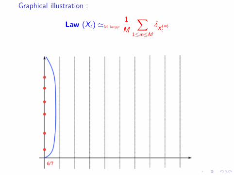
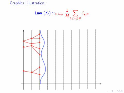
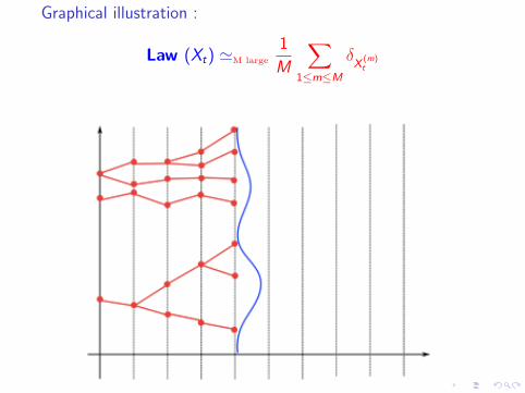
Graphical illustration :

Law (Xt) 'M large

1

M

∑1≤m≤M

δX

(m)t

I Genealogical tree model

1

N

∑1≤i≤N

δ(ξi0,n, ξ

i1,n, . . . , ξ

in,n

)︸︷︷︸i-th ancestral line

−→N→∞ Qn

Note : MCMC regularization of the tree

Qn+1path-space

= ηn+1 = ηn+1Ln+1 −→ ηn+1 = ηnKn+1,ηn Ln+1

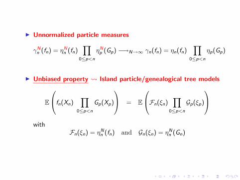
I Unnormalized particle measures

γNn (fn) = ηN

n (fn)∏

0≤p<n

ηNp (Gp) −→N→∞ γn(fn) = ηn(fn)

∏0≤p<n

ηp(Gp)

I Unbiased property Island particle/genealogical tree models

E

fn(Xn)∏

0≤p<n

Gp(Xp)

= E

Fn(ξn)∏

0≤p<n

Gp(ξp)

with

Fn(ξn) = ηNn (fn) and Gn(ξn) = ηN

n (Gn)

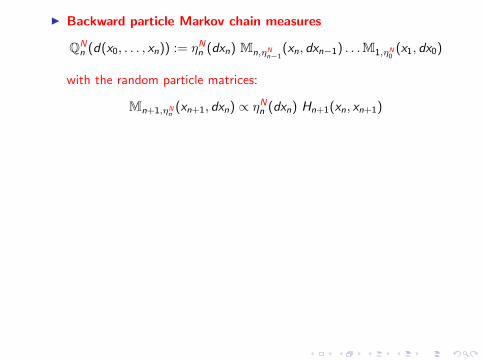
I Backward particle Markov chain measures

QNn (d(x0, . . . , xn)) := ηN

n (dxn) Mn,ηNn−1

(xn, dxn−1) . . .M1,ηN0

(x1, dx0)

with the random particle matrices:

Mn+1,ηNn

(xn+1, dxn) ∝ ηNn (dxn) Hn+1(xn, xn+1)

Finite state spaces

[{ξ0} ← {ξ1} ← . . .← {ξn}] = Complete ancestral tree

Example: Normalized additive functionals

fn(x0, . . . , xn) =1

n + 1

∑0≤p≤n

fp(xp)

⇓

QNn (fn) :=

1

n + 1

∑0≤p≤n

ηNn Mn,ηN

n−1. . .Mp+1,ηN

p(fp)︸︷︷︸

matrix operations

Matrix

Mn,ηNn−1

:=

Mn,ηNn−1

(ξ1n , ξ

1n−1) · · · Mn,ηN

n−1(ξ1

n , ξNn−1)

......

...Mn,ηN

n−1(ξN

n , ξ1n−1) · · · Mn,ηN

n−1(ξN

n , ξNn−1)

,

with the (i , j)-entry Mn,ηNn−1

(ξin, ξ

jn−1) defined by:

Mn,ηNn−1

(ξin, ξ

jn−1) =

Gn−1(ξjn−1)Hn(ξj

n−1, ξin)∑N

k=1 Gn−1(ξkn−1)Hn(ξk

n−1, ξin).

Feynman-Kac models & Particle interpretations

Applications in mathematical financePartial observation problemsStoch. interest rates, barriers, lookback style optionsAmerican optionsRisk analysis (Credit portfolio losses)Sensitivity measures (Greeks computation)


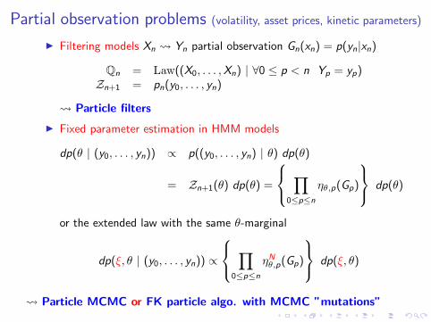
Partial observation problems (volatility, asset prices, kinetic parameters)

I Filtering models Xn Yn partial observation Gn(xn) = p(yn|xn)

Qn = Law((X0, . . . ,Xn) | ∀0 ≤ p < n Yp = yp)Zn+1 = pn(y0, . . . , yn)

Particle filters

I Fixed parameter estimation in HMM models

dp(θ | (y0, . . . , yn)) ∝ p((y0, . . . , yn) | θ) dp(θ)

= Zn+1(θ) dp(θ) =

∏0≤p≤n

ηθ,p(Gp)

dp(θ)

or the extended law with the same θ-marginal

dp(ξ, θ | (y0, . . . , yn)) ∝

∏0≤p≤n

ηNθ,p(Gp)

dp(ξ, θ)

Particle MCMC or FK particle algo. with MCMC ”mutations”

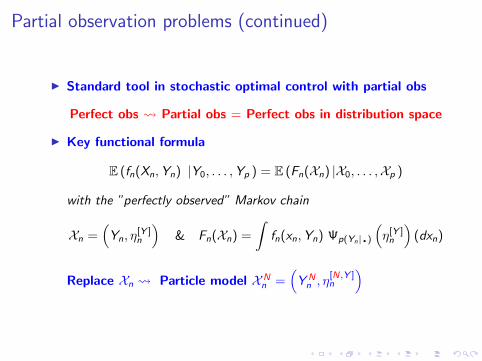
Partial observation problems (continued)

I Standard tool in stochastic optimal control with partial obs

Perfect obs Partial obs = Perfect obs in distribution space

I Key functional formula

E (fn(Xn,Yn) |Y0, . . . ,Yp ) = E (Fn(Xn) |X0, . . . ,Xp )

with the ”perfectly observed” Markov chain

Xn =(

Yn, η[Y ]n

)& Fn(Xn) =

∫fn(xn,Yn) Ψp(Yn|.)

(η[Y ]

n

)(dxn)

Replace Xn Particle model XNn =

(Y N

n , η[N,Y ]n

)

Stoch. interest rates, barriers, Lookback style options

I European call options with stoch. interest rates & barriers

fn(Xn) = (Xn − K )+ and Gn(Xn) = 1An (Xn) exp (−rn(Xn))

I Lookback style options

fn(Xn) = (Hn(Xn)− K )+ with Xn = (S0, . . . ,Sn)

Examples: 1-d Asian call option with fixed or floating strike

Hn(Xn) =1

n + 1

n∑p=0

Sp or K = 0 & Hn(Xn) =1

n + 1

n∑p=0

Sp − Sn

American optionsNotation-hypothesis :

Qn+1(x , dy) = Gn(x) Mn+1(x , dy)hyp.= Hn+1(x , y) λ(dy)

Optimal stopping time pb. supT≤n

E

fT (XT )∏

0≤p<T

Gp(Xp)

∼ Solution:

T ? = inf {0 ≤ p ≤ n : Up(Xp) ≤ fp(Xp)}

with the Snell envelop backward equation (Un = fn) :

Up(x) = fp(x) ∨∫ηp+1(dy)

dQp+1(x , .)

dηp+1(y) Up+1(y)

' fp(x) ∨ ηNp (Gp)

∫ηN

p+1(dy)Hp+1(x , y)

ηNp (Hp+1(., y))

Up+1(y)

Nb: Gn = 1 Broadie-Glasserman Monte Carlo model

American options

Variance comparison for the pricing of deep out-of-the-moneyput

Payoff K d = 1 d = 2 d = 3 d = 4 d = 5Geometric 0.95 1 1 1 1 1

Put 0.85 5 8 6 4 30.75 18 28 18 16 11

Arithmetic 0.95 1 3 3 4 5Put 0.85 5 13 24 56 100

0.75 18 71 363 866 −

Table: Variance ratio computed over 1000 runs for N = 3200 meshpoints.

American options

(a) Geometric Put with d = 4 (b) Arithmetic Put with d = 4

(c) Geometric Put with d = 5 (d) Arithmetic Put with d = 5

Risk analysis & Default tree models

Typical problem

P(Vn(Xn) ≥ a) & Law(Xn | Vn(Xn) ≥ a) ?

Importance sampling formulae:

P(Vn(Xn) ≥ a) = E

fn(Xn)∏

0≤p<n

Gp(Xp)

with the Markov chain Xn = (Xn,Xn+1) and the functions

fn(Xn) = 1Vn(Xn)≥a e−αVn(Xn) & Gp(Xp) = eα(Vp+1(Xp+1)−Vp(Xp))

Particle Importance sampling models ⊕ Default tree models

Risk analysis & Default tree models

Default distribution of a portfolio of 125 stocks

Kinetic parameter derivatives

Derivation FK models = FK Integration w.r.t. additive functionals

θ ∈ Rd=1 7→ Qθn (xn−1, dxn) = G θ

n−1(x) Mθn (x , dy) = Hθ

n (xn−1, xn) λn(dxn)

⇒ ∂

∂θE

fn(X θ0 , . . . ,X

θn )

∏0≤p<n

G θp (X θ

p )

∝ Qθn(fn × Γθn)

with the additive functional

Γθn(x0, . . . , xn) =∑

1≤p≤n

∂

∂θlog Hθ

p (xp−1, xp)

Particle backward Markov chains or Genealogical tree models

Parameter derivatives (continued)

I Greeks computation: (vega,rho) = (volatility,drift) θ-variations

I θ-variations of barrier levels or smooth penalty type functions:

d = 1 & a smooth θ 7→ (G θn ,M

θn ) = (G θ

n ,Mn)

∂

∂θlogZθn = Qθ

n(Γθn) &∂

∂θQθ

n(fn) = Qθn(fn

[Γθn −Qθ

n(Γθn)])

with the additive functional

Γθn(x0, . . . , xn) =∑

0≤p<n

∂

∂θlog G θ

p (xp)

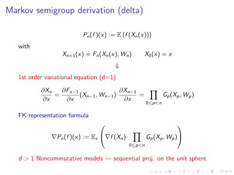
Markov semigroup derivation (delta)

Pn(f )(x) := E (f (Xn(x)))

withXn+1(x) = Fn(Xn(x),Wn) X0(x) = x

⇓

1st order variational equation (d=1)

∂Xn

∂x=∂Fn−1

∂x(Xn−1,Wn−1)

∂Xn−1

∂x=

∏0≤p<n

Gp(Xp,Wp)

FK-representation formula

∇Pn(f )(x) := Ex

∇f (Xn)∏

0≤p<n

Gp(Xp,Wp)

d > 1 Noncommutative models sequential proj. on the unit sphere

Feynman-Kac models & Particle interpretations

Applications in mathematical finance


Cts (c1, c2) ∼ (bias,variance), independent of the time parameterTest functions ‖fn‖ ∨ ‖fn‖ ≤ 1, c universal constant, ε ∈ {−1,+1}

∀ (x ≥ 0, n ≥ 0,N ≥ 1), the probability of any of the following events isgreater than 1− e−x

[ηN

n − ηn

](fn) ≤ c1

N

(1 + x +

√x)

+c2√N

√x

ε

nlogZN

n

Zn≤ c1

N

(1 + x +

√x)

+c2√N

√x

[ηN

n −Qn

](fn) ≤ c1

n + 1

N

(1 + x +

√x)

+ c2

√(n + 1)

N

√x

Nb: Similar results at the empirical process level over classes of functions

Backward particle models

Cts (c1, c2) ∼ (bias,variance), independent of the time parameterfn normalized additive functional with ‖fp‖ ≤ 1, c universal constant

∀ (x ≥ 0, n ≥ 0,N ≥ 1), the probability of any of the following events isgreater than 1− e−x

[QN

n −Qn

](fn) ≤ c1

1

N(1 + (x +

√x)) + c2

√x

N(n + 1)

and

supa∈Rd

∣∣QNn (fa,n)−Qn(fa,n)

∣∣ ≤ c

√d

N(x + 1)

with fa,n normalized additive functional w.r.t. fp = 1(−∞,a], a ∈ Rd = En

.

ReferencesI joint work with R. Carmona, P. Del Moral and N. Oudjane, An introduction to particle methods in

Finance. Numerical Methods in Finance, Springer (2012).

I joint work with P. Del Moral and L. Wu, On the concentration properties of Interacting particleprocesses, Foundations and Trends in Machine Learning, vol. 3, nos. 3–4, pp. 225–389, 2012.

I joint work with P. Del Moral, N. Oudjane, Br. Remillard. On the Robustness of the Snell envelope.SIAM J. Finan. Math., Vol. 2, pp. 587–626 , 2011.

I joint work with P. Del Moral, N. Oudjane, Snell envelope with small probability criteria, to appear inApplied Mathematics & Optimization.

I R.Carmona, S. Crepey. Importance sampling and interacting particle systems for the estimation ofcredit portfolios loss distribution. International Journal of Theoretical and Applied Finance, to appear(2011).

I R. Carmona, J.-P. Fouque, and D. Vestal. Interacting particle systems for the computation of rarecredit portfolio losses, Finance and Stochastics, vol. 13, no. 4, pp. 613-633 (2009).Particle Markov chain Monte Carlo methods. (with discussion), Journal Royal Statistical Society B.,vol. 72, no. 3, pp. 269-342 (2010).

I P. Del Moral, A. Doucet and A. Jasra. Sequential Monte Carlo samplers. J. Royal Statist. Soc. B,vol. 68, pp. 411–436, 2006.

I P. Del Moral and J. Garnier. Genealogical particle analysis of rare events. Annals of AppliedProbability, vol. 15, no. 4, pp. 2496-2534 (2005).

I P. Del Moral, A.Doucet, S.S.Singh, A Backward Particle Interpretation of Feynman-Kac Formulae.M2AN, 44(5), pp. 947-976 (2010).

I P. Del Moral, A.Doucet, S.S.Singh, Uniform Stability of a Particle Approximation of the Optimal FilterDerivative http://arxiv.org/abs/1106.2525 (2011).

I P. Del Moral and E. Rio. Concentration Inequalities for Mean Field Particle Models. Annals of AppliedProbability, vol.21, no.3, pp.1017-1052 (2011).

I P. Del Moral, Feynman-Kac Formulae: Genealogical and Interacting Particle Systems with Applications,Springer-Verlag, Series Probability & Applications (2004).

I P. Del Moral and A. Doucet. Sequential Monte Carlo and Genetic particle models. Theory andPractice. Chapman & Hall, Series Statistics & Applied Probability (2012).

An introduction to particle methods in mathematical finance

Documents

Transcript of An introduction to particle methods in mathematical finance