HAL Id: hal-02268787https://hal.archives-ouvertes.fr/hal-02268787

Submitted on 21 Aug 2019

HAL is a multi-disciplinary open accessarchive for the deposit and dissemination of sci-entific research documents, whether they are pub-lished or not. The documents may come fromteaching and research institutions in France orabroad, or from public or private research centers.

L’archive ouverte pluridisciplinaire HAL, estdestinée au dépôt et à la diffusion de documentsscientifiques de niveau recherche, publiés ou non,émanant des établissements d’enseignement et derecherche français ou étrangers, des laboratoirespublics ou privés.

An introduction to p-adic period ringsXavier Caruso

To cite this version:Xavier Caruso. An introduction to p-adic period rings. Société Mathématique de France. An excursioninto p-adic Hodge theory: from foundations to recent trends, 54, 2019, Panoramas et Synthèses, 978-2-85629-913-5. hal-02268787

An introduction to p-adic period rings

Xavier Caruso

August 21, 2019

Abstract

This paper is the augmented notes of a course I gave jointly with Laurent Berger in

Rennes in 2014. Its aim was to introduce the periods rings Bcrys and BdR and state severalcomparison theorems between etale and crystalline or de Rham cohomologies for p-adic

varieties.

Contents

1 From Hodge decomposition to Galois representations 3

1.1 Setting and preliminaries . . . . . . . . . . . . . . . . . . . . . . . . . . . . . . . 3

1.2 Motivations: p-divisible groups and etale cohomology . . . . . . . . . . . . . . . . 6

1.3 Notion of semi-linear representations . . . . . . . . . . . . . . . . . . . . . . . . . 8

1.4 Fontaine’s strategy . . . . . . . . . . . . . . . . . . . . . . . . . . . . . . . . . . . 10

2 The first period ring: Cp 13

2.1 Ramification in Zp-extensions . . . . . . . . . . . . . . . . . . . . . . . . . . . . . 14

2.2 Cp-admissibility . . . . . . . . . . . . . . . . . . . . . . . . . . . . . . . . . . . . . 18

2.3 Complement: Sen’s theory . . . . . . . . . . . . . . . . . . . . . . . . . . . . . . . 23

3 Two refined period rings: Bcrys and BdR 27

3.1 Preliminaries: the ring B+inf

. . . . . . . . . . . . . . . . . . . . . . . . . . . . . . 30

3.2 The ring Bcrys and some variants . . . . . . . . . . . . . . . . . . . . . . . . . . . 35

3.3 The de Rham filtration and the field BdR . . . . . . . . . . . . . . . . . . . . . . . 39

3.4 Bcrys and BdR as period rings . . . . . . . . . . . . . . . . . . . . . . . . . . . . . 44

4 Crystalline and de Rham representations 46

4.1 Comparison theorems: statements . . . . . . . . . . . . . . . . . . . . . . . . . . 46

4.2 More on de Rham representations . . . . . . . . . . . . . . . . . . . . . . . . . . . 50

4.3 More on crystalline representations . . . . . . . . . . . . . . . . . . . . . . . . . . 52

Introduction

In algebraic geometry, the word period often refers to a complex number that can be expressed

as an integral of an algebraic function over an algebraic domain. One of the simplest periods is

2iπ =∫

γdtt , where γ is the unit circle in the complex plane. Equivalently, a period can be seen

as an entry of the matrix (in rational bases) of the de Rham isomorphism:

C⊗Q Hrsing(X(C),Q) ≃ C⊗K Hr

dR(X) (1)

for an algebraic varietyX defined over a number fieldK. (HereHrsing is the singular cohomology

and HrdR denotes the algebraic de Rham cohomology.)

1

The initial motivation of p-adic Hodge theory is the will to design a relevant p-adic analogue

of the notion of periods. To this end, our first need is to find a suitable p-adic generalization of

the isomorphism (1). In the p-adic setting, the singular cohomology is no longer relevant; it has

to be replaced by the etale cohomology. Thus, what we need is a ring B allowing for a canonical

isomorphism:

B ⊗Qp Hret(XK ,Qp) ≃ B ⊗K Hr

dR(X) (2)

when K is now a finite extension of Qp and X is a variety defined over K. Of course, the first

natural candidate one thinks at is B = Cp, the p-adic completion of an algebraic closure K of K.

Unfortunately, this first period ring does not totally fill our requirements. More precisely, it turns

out that Cp ⊗Qp Hret(XK ,Qp) is isomorphic to the graded module (for the de Rham filtration) of

Cp ⊗K HrdR(X) but not to Cp ⊗K Hr

dR(X) itself. The main objective of this lecture is to detail

the construction of two periods rings, namely Bcrys and BdR, allowing for the isomorphism (2)

under some additional assumptions on the variety X. The ring BdR (which is the bigger one) is

often called the ring of p-adic periods.

Another important aspect of p-adic period rings concerns the Galois structure ofHret(XK ,Qp).

Indeed, we shall see that the mere existence of the isomorphism (2) usually has strong conse-

quences on the Galois module Hret(XK ,Qp). In order to give depth to this observation, Fontaine

developed a general formalism for studying and classifying general Galois representations through

the notion of period rings. A large part of this article focuses on the Galois aspects.

Structure of the article. §1 serves as a second long introduction to this article; two results

which can be considered as the seeds of p-adic Hodge theory are presented and discussed. The

first one is due to Tate and provides a Hodge-like decomposition of the Tate module of a p-divisible group in the spirit of the isomorphism (2). The second result is a classification theorem

of p-divisible groups by Fontaine. Fontaine’s general formalism for studying Galois representa-

tions is also introduced in this section.

In §2, we investigate to what extent Cp meets the expected properties of a period ring. We

adopt the point of view of Galois representations, which means concretely that we will con-

centrate on isolating those Galois representations that are susceptible to sit in an isomorphism

of the form (2) when B = Cp. This study will lead eventually to the notion of Hodge–Tate

representations, which is related to the Hodge-like decompositions of cohomology presented

in §1.

In §3, we review the construction of the period rings Bcrys and BdR; it is the heart of the

article but also its most technical part. Finally, in §4, we state several comparison theorems

between etale and de Rham cohomologies. We also show how the rings Bcrys and BdR intervene

in the classification of Galois representations, through the notions of crystalline and de Rham

representations.

Some advice to the reader. Although we will give frequently reminders, we assume that

the reader is familiar with the general theory of local fields as presented in [39], Chapter 1–

4. A minimal knowledge of local class field theory [39] and of the theory of p-adic analytic

functions [33] is also welcome, while not rigourously needed.

To the impatient reader who is afraid by the length of this article and is not interested in

the details of the proofs (at least in first reading) but only by a general outline of p-adic Hodge

theory, we advise to read §1, then the introduction of §3 until §3.1 and then finally §4.

Acknowledgement. The author is grateful to the editorial board of Panoramas et Syntheses,

and especially to Ariane Mezard, who encourages him to finalize this article after many years.

He also warmly thanks Olivier Brinon for sharing with him his notes of a master course on p-adic

Hodge theory he taught in Bordeaux.

2

Notations. Throughout this article, the letter p will refer to a fixed prime number. We use

the notation Zp (resp. Qp) for the ring of p-adic integers (resp. the field of p-adic numbers).

We recall that Qp = Frac Zp = Zp[1p ]. Let also Fp denote the finite field with p elements, i.e.

Fp = Z/pZ.

If A in a ring, we denote by A× the multiplicative group of invertible elements in A.

1 From Hodge decomposition to Galois representations

After having recalled some basic facts about local fields in §1.1, we discuss in §1.2 two families

of results which are the seeds of p-adic Hodge theory. Both of them are of geometric nature.

The first one concerns the classification of p-divisible groups over the ring of integers of a local

field, while the second one concerns the Hodge-like decomposition of the etale cohomology of

varieties defined over local fields. From this presentation, the need to have a good tannakian

formalism emerges.

Carried by this idea, we move from geometry to the theory of representations and focus

on tensor products and scalar extensions. Eventually, this will lead us to the notion of B-

admissibility, which is the key concept in Fontaine’s vision of p-adic Hodge theory. Finally, we

briefly discuss the applications we will develop in the forthcoming sections: usingB-admissibility,

we introduce the notions of crystalline, semi-stable and de Rham representations and explain

rapidly how the general theory can help for studying these classes of representations.

1.1 Setting and preliminaries

Let K be a finite extension1 of Qp. Let vp : K → Q ⊔ +∞ be the valuation on K normalized

by vp(p) = 1. By our assumptions, vp(K×) is a discrete subgroup of Q containing Z; hence it

is equal to 1eZ for some positive integer e. We recall that this integer e is called the absolute

ramification index of K. A uniformizer of K is an element of minimal positive valuation, that is

of valuation 1e . We fix a uniformizer π of K.

Let OK be the ring of integers of K, that is the subring of K consisting of elements with

nonnegative valuation. We recall that OK is a local ring whose maximal ideal mK consists of

elements with positive valuation. The residue field k of K is, by definition, the quotient OK/mK .

Under our assumptions, k is a finite field of characteristic p.Let W (k) denote the ring of Witt vectors with coefficients in k. Set K0 = FracW (k). By the

general theory of Witt vectors, there exists a canonical embedding K0 → K. Moreover, through

this embedding, K appears as a finite totally ramified extension of K0 of degree e. Therefore,

K0 is the maximal subextension of K which is unramified over Qp.

1.1.1 The absolute Galois group of K

We choose and fix once for all an algebraic closure K of K. We recall that the valuation vpextends uniquely to K, so that we can talk about the ring of integers OK of K. This ring is a

local ring whose maximal ideal will be denoted by mK . The quotient OK/mK is identified with

an algebraic closure of k; it will be denoted k in the sequel.

Let GK = Gal(K/K) be the absolute Galois group of K. Any element of GK acts by isometry

on K and therefore stabilizes OK and mK . It thus acts on the residue field k. This defines a

group homomorphism GK → Gal(k/k), which is surjective. The kernel of this morphism is the

inertia subgroup; we shall denote it by IK in the sequel. The subextension of K cut out by IK

1We could have considered a more general setting where K is a complete discrete valued field of characteristic

0 with perfect residue field of characteristic p. All the results presented in the paper extend to this more general

setting. However the case of finite extensions of Qp is the main case of interest and restricting to this case simplifies

the exposition at several points.

3

is the maximal unramified extension of K; we will denote it by Kur. Summarizing the above

discussion, we find that GK sits in the following exact sequence:

1 −→ IK −→ GK −→ Gal(k/k)→ 1.

The structure of Gal(k/k) is also known: if k has cardinality q, Gal(k/k) is the profinite group

generated by the Frobenius Frobq : x 7→ xq.The structure of IK can be further precised. Indeed a simple application of Hensel’s lemma

shows that any finite extension of Kur whose degree is not divisible by p has the form Kur[ n√π].

The union of all these extensions is called K tr; it is the maximal tamely ramified extension of K.

Since Kur contains all n-th roots of unity for n ∤ p (cf the paragraph The cyclotomic extension

below for more details), the extension K tr/Kur is Galois and its Galois group is identified with

lim←−n,p∤n Z/nZ ≃∏

ℓ 6=p Zℓ. Moreover, any finite extension of K tr has degree pm for some integer

m. On the Galois side, these properties imply that the closed subgroup of IK corresponding to

the extension K tr is the unique pro-p-Sylow of IK (which is then a normal subgroup) and that

IK sits in the following exact sequence:

1 −→ PK −→ IK −→ lim←−n,p∤n

Z/nZ→ 1

where PK denotes the pro-p-Sylow of IK .

1.1.2 The cyclotomic extension

The cyclotomic extension of K plays a quite important role in p-adic Hodge theory. So we

take some time to recall its most important properties. Let µn ∈ K be a primitive n-th root of

unity. We recall that, by definition, the cyclotomic extension of K is the subextension Kcycl of Kgenerated by the µn’s.

The extension K(µn)/K is Galois and its Galois group canonically embeds into (Z/nZ)×

through the map χn : Gal(K(µn)/K)→ (Z/nZ)× defined by the relation χn(µn) = µχn(g)n for all

g ∈ Gal(K(µn)/K). We draw the reader’s attention to the fact that χn is in general not surjective

although it is for all n when K = Qp.

When n is coprime with p, the extension K(µn)/K is unramified since the polynomial Xn−1splits over k. In this case, K(µn) appears as a subextension of Kur. On the other hand, when

n = pr is a power of p, the extension K(µpr)/K is totally ramified. This dichotomy motivates

the introduction of the two following infinite extensions of K:

Kp′-cycl =⋃

n,p∤n

K(µn) and Kp-cycl =⋃

r≥0

K(µpr).

The first one is actually equal to Kur since, at the level of residue fields, k is obtained by k by

adding all pn-th roots of unity for p ∤ n. As for Kp-cycl, it is linearly disjoint from Kur. It is

sometimes called the p-cyclotomic extension of K. Clearly, the cyclotomic extension of K is the

compositum of Kur and Kp-cycl.

Let us review briefly the Galois properties of Kp-cycl. First of all, we notice that Kp-cycl/K is

Galois. Its Galois group is equipped with an injective group homomorphism χp∞ : Gal(Kp-cycl/K)→Z×p which is characterized by the relation gµpm = µ

χp∞(g)pm (for all g ∈ Gal(Kp-cycl/K) andm ≥ 1).

Let χcycl : GK → Z×p be the homomorphism obtained by precomposing χp∞ with the canonical

surjection GK → Gal(Kp-cycl/K). We shall often see χcycl as a character and will call it the

(p-adic) cyclotomic character. As χp∞, it is determined by the relation:

gµpm = µχcycl(g)pm for all g ∈ GK and m ≥ 1.

4

By construction, the extension corresponding to kerχcycl is Kp-cycl and, more generally, for all

positive integer r, the extension corresponding to ker(χcycl mod pr) is K(µpr).The logarithm defines a group morphism Z×

p → Zp where the group structure on the target

is given by the addition. It sits in the exact sequence:

1 −→ F×p

[·]−→ Z×p

log−→ Zp −→ 1 (3)

where [·] denotes the Teichmuller representative function. This sequence is split since a retrac-

tion of F×p → Z×

p is simply the canonical projection. Therefore Z×p is canonically isomorphic to

F×p × Zp. Restricting (3) to the image of χcycl, we find that Gal(Kp-cycl/K) sits in another exact

sequence which reads as follows:

1 −→ H −→ Gal(Kp-cycl/K)logχcycl−→ pr0Zp −→ 1.

Here r0 is a nonnegative integer and H can be identified as a subgroup of F×p and thus is

cyclic of order divisible by p−1. The above sequence splits, so that Gal(Kp-cycl/K) is canonically

isomorphic to a direct product H × pr0Zp ≃ H × Zp.The subextension of Kp-cycl cut out by the factor Zp is nothing but K(µp). It is also the

maximal tamely ramified subextension of Kp-cycl. The Galois group of Kp-cycl/K(µp) is canoni-

cally isomorphic to Zp via the additive character p−r0 log χcycl. We say that Kp-cycl/K(µp) is a

Zp-extension. The fact that Gal(Kp-cycl/K) splits as a direct product means that this extension

descends to K; in particular, K itself admits a Zp-extension.

1.1.3 Characters of GQp

The representation theory of GK is the main object of interest in this article. Among all represen-

tations ofGK , the simplest ones are of course characters, which are representations of dimension

1. We have actually already seen an example of such character: the cyclotomic character χcycl.

From χcycl, we can build the following other character:

ωcycl : GKχcycl−→ Z×

pmod p−→ F×

p[·]−→ Z×

p

where the last map takes an element to its Teichmuller representative. We observe that ωcycl is a

finite order character, whose order divides p−1. When K = Qp, the order of ωcycl is exactly p−1.

Another quite important family of characters are unramified characters, that are those charac-

ters which are trivial on the inertia subgroup. Since GK/IK ≃ Gal(k/k) is procyclic, continuous

unramified characters are easy to describe: they are all of the form

µλ : GK −→ GK/IK ≃ Gal(k/k)Frobq 7→λ−→ Z×

p

for λ varying in Z×p .

Using local class field theory (cf [39]), it is possible to describe explicitely all characters of

GK . Indeed such characters all factor through the abelianization of GK , which is closely related

to K× through the Artin reciprocity map. When K = Qp, this answer is given by the following

proposition.

Proposition 1.1.1. We assume p > 2. Let χ be a character of GK with values in Q×p .

Then, there exist unique λ ∈ Z×p , a ∈ Zp and b ∈ Z/(p−1)Z such that χ = µλ · χacycl · ωbcycl.

Proof. We first observe that, by compacity, χ must take its values in Z×p . By the Kronecker–Weber

theorem, we know that the maximal abelian extension of Qp is the cyclotomic extension. There-

fore χ has to factor through Gal(Qp,cycl/Qp). In particular, χ|IQpfactors through Gal(Qp,cycl/Q

urp )

which is isomorphic to Z×p by the cyclotomic character. Consequently, χ|IQp

= h χcycl for

5

some group homomorphism h : Z×p → Z×

p . Moreover, when p > 2, we have an isomorphism

Z×p ≃ F×

p × Zp, x 7→ (x mod p, log x), the inverse being given by (a, b) 7→ [a]· exp b where [a]denotes the Teichmuller representative of a. From this description, we derive that there exist

a ∈ Zp and b ∈ Z/(p−1)Z such that h(x) = xa · [x mod p]b for x ∈ Z×p . Thus χIQp

= χacycl · ωbcycl.

The character χ · χ−acycl· ω−b

cyclis then unramified. Thus it must be of the form µλ for some λ ∈ Z×

p .

The proposition is proved.

1.2 Motivations: p-divisible groups and etale cohomology

The starting point of p-adic Hodge theory is Tate’s paper of 1966 on p-divisible groups [40].

In this seminal article, Tate establishes a Hodge-like decomposition of the Tate module of a p-divisible group on OK . More precisely, let G be a p-divisible group on OK . We define the Tate

module of G by TpG = lim←−n G[pn](K). Observe that TpG is naturally endowed with an action of

GK . The algebraic structure of TpG is well-known: it is a free module of finite rank over Zp. Set

VpG = Qp ⊗Zp TpG. Then, Tate proves the following Hodge-like GK -equivariant decomposition:

Cp ⊗Qp VpG ≃(

Cp ⊗OKωG∨

)

⊕(

Cp(χ−1cycl

)⊗OKω∨G

)

. (4)

Here G∨ is the Cartier dual of G, the construction ω− refers to the cotangent space at the origin

and Cp(χ−1cycl

) is Cpe endowed with the action g(λe) = gλ · χ−1cycl

(g) · e (for g ∈ GK and λ ∈Cp). Note that the Galois action is trivial over ωG∨ and ω∨

G . The isomorphism (4) then reveals

the Galois action on the Tate module. Tate’s theorem implies in particular that, when A is an

abelian variety over K with good reduction, the etale cohomology of A admits the following

decomposition:

Cp ⊗Qp H1et(AK ,Qp) ≃

(

Cp ⊗K H1(A,OA))

⊕(

Cp(χ−1cycl

)⊗K H0(A,ΩA/K))

. (5)

were AK = Spec K ×Spec K A, OA is the structural sheaf of A and ΩA/K is the sheaf of Kahler

differentials of A over K. We refer to Freixas’ lecture in this volume [25] for a more detailed

discussion—including a sketch of the proof—about Tate’s theorem.

After Tate’s results, p-divisible groups over various bases were studied intensively. In the

1970’s, Fontaine [18] obtained a complete classification of p-divisible groups and finite flat group

schemes over OK when K/Qp is unramified. The starting point of Fontaine’s theorem is the

classification of p-divisible groups over perfect fields of characteristic p in terms of Dieudonne

modules [13]. Let us recall briefly how it works. If Gk is a p-divisible group over k, we define

M(Gk) = Homgr(Gk, CWk) (6)

where CWk is the functor of Witt covectors and the notations Homgr means that we are consid-

ering the set of all natural transformations preserving the group structure. The space M(Gk)is a Dieudonne module. This means that it is a module over W (k) endowed with a Frobe-

nius F (which is a semi-linear endomorphism with respect to the Frobenius on W (k)) and a

Verschiebung V (which is a semi-linear endormorphism with respect to the inverse of the Frobe-

nius) with the property that FV = V F = p. One can show that M realizes an anti-equivalence

of categories between the category of p-divisible groups over k and that of finite free Dieudonne

modules over W (k), the inverse functor being given by the formula

Gk(A) = HomW (k),F,V

(

M,CW (A))

for any k-algebra A

which is quite similar to (6). Now, if G is a p-divisible over OK with special fibre Gk, Fontaine

constructs a submodule L(G) ⊂ M(Gk) and demonstrates that it obeys to a certain list of prop-

erties. Taking these properties as axioms, Fontaine introduces the notion of Honda systems and

proves that the association G 7→ (M(Gk), L(G)) is an anti-equivalence of categories between the

6

category of p-divisible groups over OK and the category of finite free Honda systems over W (k).Moreover, Fontaine establishes a compact formula for the inverse functor. This formula reads:

VpG = Qp ⊗Zp Homhonda

(

(M(Gk), L(G)), (B, LB))

(7)

where the notation Homhonda means that we are taking the morphisms in the category of Honda

system and the target (B, LB) is a special Honda system2 (the letter B refers to the mathe-

matician Barsotti, who first studied p-divisible groups using this kind of techniques). Moreover,

(B, LB) is endowed with an action of GK , from which we can recover the GK -action on VpG.

Compared to Tate’s decomposition formula (4), Fontaine’s result is more precise because it de-

scribes the Tate module VpG itself, whereas Tate’s result only concerns its scalar extension to Cp.For many complements about Fontaine’s classification results, we refer to [18, 12].

About ten years later, in 1981, Fontaine came back to Tate’s decomposition isomorphism (5)and

gave a different proof of it (which is sketched in Freixas’ lecture in this volume [25]), relaxing

at the same time the assumption of good reduction. He also became interested in generalizing

Tate’s decomposition theorem to higher cohomology group (i.e. Hret(AK ,Qp) with r > 1) and

other types of varieties. Moreover, noticing that the right hand side of (5) is the graded module

of the de Rham cohomology, one may wonder if one can make the isomorphism (5) more pre-

cise and relate the etale cohomology with the de Rham cohomology equipped with its filtration.

All these questions had been a strong motivation for the development of p-adic Hodge theory

for many years. Nowadays, all of them are solved: it has been proved independently by Falt-

ings [15] and Tsuji [41] that BdR ⊗Qp Hret(XK ,Qp) ≃ BdR ⊗Qp H

rdR(X) whenever X is a proper

smooth variety over K and r is a nonnegative integer. Here BdR is the so-called field of p-adic

periods. We will introduce it in this article in §3. Taking the grading in the above isomorphism,

we get the following Hodge-like decomposition:

Cp ⊗Qp Hret(XK ,Qp) ≃

⊕

a+b=r

Cp(χ−acycl

)⊗K Hb(X,ΩaX/K).

We will come back to these results in §4.1.

Finally, it is interesting to confront the two directions of research discussed above, namely

classification of p-divisible groups and Hodge-like decomposition theorems. As already men-

tioned, one important feature of the isomorphism (7) is the fact that it gives a complete de-

scription of the Galois action on the Tate module. On the other hand, it is apparent that Honda

systems have important limitations: by design, they can only deal with Tate modules, that is,

roughly speaking, with the first cohomology group. Analyzing carefully the situation, Fontaine

realized that what is missing to Honda systems is a good tannakian formalism (which is, of

course, a key point in the line of Hodge-like decomposition theorems). In more crude terms,

the fact that we are limited to the H1et should be understood as a reflection of the fact that we

are missing a good notion of tensor product on p-divisible groups. As explained in the introduc-

tion of [19], the period ring Bcrys and the afferent notion of crystalline representations actually

emerge when trying to conceal the theory of Honda systems with the tannakian formalism in-

spired from the Hodge-like decomposition theorems we have presented above.

All the developments we will present in the sequel are stamped by this simple idea that one

wants to keep apparent the tannakian structure (i.e. the tensor product) everywhere and, even,

to use it as a main tool. The natural framework in which the theory grows is then that of Galois

representations, which has a strong tannakian structure.

2Its construction is subtle and we will not give it here. However, we would like to encourage the reader to look

at it in Fontaine’s paper [18, Chap. V, §1] because it is instructive to realize that it is actually quite close to the

construction of the periods BdR and Bcrys we shall detail in §3.

7

1.3 Notion of semi-linear representations

The Hodge-like decomposition theorems discussed previously motivate the study of representa-

tions of the form W = Cp ⊗Qp V where V is a given Qp-representation of GK . Since GK does

act on Cp, we observe that W is not a Cp-linear representation in the usual sense. Instead, it is

a so-called semi-linear representation. The aim of this subsection is to introduce and study this

notion.

1.3.1 Definitions

In what follows, we let G be a topological group3 and B be a topological ring equipped with a

continuous4 action of G, which is compatible with the ring structure, i.e. g · (a + b) = ga + gband g · (ab) = ga gb for all g ∈ G and a, b ∈ B.

Definition 1.3.1. A B-semi-linear representation of G is the datum of a B-module W equipped

with a continuous action of G such that:

g · (x+ y) = gx+ gy and g · (ax) = ga · gx

for all g ∈ G, a ∈ B and x, y ∈W .

Clearly, if G acts trivially on B, the notion of B-semi-linear representation of G agrees with

the usual notion of B-linear representation of G.

By our assumptions, B itself (endowed with its G-action) is a B-semi-linear representation

of G. Similarly we can turn Bn into a B-semi-linear representation by letting G act coordinate

by coordinate. The latter representation will be called the trivial representation of dimension n.

If W1 and W2 are two B-semi-linear representations of G, a morphism W1 → W2 is a B-

linear mapping which commutes with the action of G. With this definition, we can form the

category of B-semi-linear representations of G (for G and B fixed). In the sequel we will simply

denote it RepB(G). It is easily seen that RepB(G) is an abelian category. It is moreover endowed

with a notion of tensor product and internal hom: if W1 and W2 are objects of RepB(G), then

W1 ⊗BW2 (equipped with the action g · (x⊗ y) = gx⊗ gy) and HomB(W1,W2) (equipped with

the action gϕ : x 7→ gϕ(g−1x)) are also.

Scalar extension There is also a natural notion of scalar extension in the framework of semi-

linear representations. To explain it, let us consider a closed subring C of B, which is stable

under the action of G. Then the notion of C-semi-linear representations of G makes sense and

there is a canonical functor RepC(G)→ RepB(G) taking W to B ⊗C W .

The latter construction is quite interesting because it allows us to build semi-linear repre-

sentations from classical representations. Indeed, assume that we are given a field E and we

have chosen G and B is such a way that B is an algebra over E and G acts trivially on E. (As

an example, B could be a Galois extension of E with G = Gal(B/E).) The scalar extension

then defines a functor RepE(G)→ RepB(G). Moreover, since the action of G on E is trivial, the

category RepE(G) is just the category of E-linear representations of G. In more concrete terms,

if V is a classical representation of G defined over E, then W = B ⊗E V is a B-semi-linear

representation. This is actually the prototype of all the semi-linear representations we are going

to consider in this article.

Specializing the previous recipe to 1-dimensional representations, we obtain a way to con-

struct semi-linear representations of G from characters of G. Concretely, if χ : G → E× is a

3In the application we have in mind, G will be the absolute Galois group of a p-adic field. However, for now, it is

better to allow more flexibility and let G be an arbitrary topological group.4By continuous, we mean that the map G×B → B, (g, x) 7→ gx is continuous.

8

multiplicative character, we will denote by B(χ) the 1-dimensional representation generated by

a vector eχ on which G acts by geχ = χ(g) · eχ for all g ∈ G. By semi-linearity, we then have

g(a eχ) = ga · χ(g) eχ

for all g ∈ G and a ∈ B.

1.3.2 Recognizing the trivial representation

We keep the setup of the previous subsection: G is a topological group which acts continuously

on a topological ring B.

Definition 1.3.2. A B-semi-linear representation of G is trivial if it is isomorphic to the trivial

representation Bd for some positive integer d.

While it is in general easy to recognize when a linear representation is trivial (it suffices

to check that G acts trivially on each vector of the representation), the task becomes more

complicated in the context of semi-linear representations. Indeed, coming back to the definition,

we see that a B-semi-linear representation of G is trivial if and only if it admits a basis of vectors

which are fixed byG. In particular, it is quite possible that a nontrivial semi-linear representation

becomes trivial after scalar extension. The latter remark is in fact the starting point of Fontaine’s

strategy for classifying Galois representations.

We will discuss Fontaine’s strategy in much more details in §1.4. Before this, we have to

introduce further notations. Given W ∈ RepB(G), we denote by WG the subset of W consisting

of fixed points under G, that is the subset of elements x ∈ W such that gx = x for all g ∈ G.

Clearly WG is a module over BG. Moreover scalar extension provides a canonical morphism in

RepB(G):αW : B ⊗BG WG −→W.

This morphism is useful for recognizing trivial representations. Indeed it is clearly an isomor-

phism when W is trivial in the sense of Definition 1.3.2 (since (Bd)G = (BG)d) and the converse

also holds true when W and WG are free of finite rank over B and BG respectively.

1.3.3 Hilbert’s theorem 90

As an introduction to Fontaine’s strategy, we propose to discuss an easy case where trivial semi-

linear representations do appear, while they were not expected at first glance. The setting here

is the following. We assume that B is a field and, in order to limit confusion, we will call it

L. We assume also that G is a finite group, endowed with the discrete topology. Under these

assumptions, LG is a subfield of L and the extension L/LG is finite and Galois with Galois

group G.

Theorem 1.3.3. We keep the notations and assumptions above.

For all W ∈ RepL(G), the following assertions hold:

1. the morphism αW is surjective,

2. if W is finite dimensional over L, then αW is an isomorphism, i.e. W is trivial.

Proof. Let λ1, . . . , λn be a basis of L over LG. By Artin’s linear independence theorem, there exist

constants µ1, . . . , µn ∈ L such that∑n

i=1 µig(λi) is 1 if g is the identity and 0 otherwise. Define

the trace function T : W → W by T (x) =∑

g∈G gx. One easily checks that T takes its values in

WG. Moreover, for the particular µi’s we have introduced earlier, we have∑n

i=1 µiT (λix) = xfor all x ∈W . This shows the surjectivity of αW .

We now assume that W is finite dimensional over L. The proof of injectivity is quite similar

to the proof of Artin’s linear independence theorem. It is enough to check that every finite family

9

of elements of WG which is linearly independent over LG remains linearly independent over L.

Let then (x1, . . . , xm) be a linearly independent family over LG with xi ∈ WG for all i. We

assume by contradiction that there exists a nontrivial relation of linear dependance of the form:

a1x1 + a2x2 + · · ·+ amxm = 0 (8)

with ai ∈ L. We choose such a relation so that the number of nonzero ai’s is minimal. Up to

reindexing the ai’s and rescaling the relation, we may assume that a1 = 1. Let g ∈ G. Applying

(g − id) to (8), we get the relation (ga2 − a2)x2 + · · ·+ (gam − am)xm = 0 which is shorter than

(8). From our minimality assumption, we deduce that gai = ai for all i ≥ 2. Since this is valid

for all g ∈ G, we deduce that the linear dependance relation (8) has coefficients in LG. This

is a contradiction since we have assumed that the family (x1, . . . , xm) is linearly independent

over LG.

Remark 1.3.4. Theorem 1.3.3 is often referred to as Hilbert’s theorem 90. The reason is that

it can be rephrased in the language of group cohomology, then asserting that H1(G,GLd(L)) is

reduced to one element. This latter statement is an extension of the classical Hilbert’s theorem

90 to higher d.

Example 1.3.5. We emphasize that Theorem 1.3.3 does not hold in general when G = Gal(L/K)where L/K is an infinite extension and G is equipped with its natural profinite topology. As

an example, take G = GQp = Gal(Qp/Qp) and let it act on L = Qp. The fixed subfield LG

is Qp. Consider the semi-linear representation Qp(χcycl) where we recall that χcycl denotes the

cyclotomic character Gal(Qp/Qp) → Z×p ⊂ Q×

p . We claim that Qp(χcycl) is not isomorphic to Qp

in the category RepQp(GQp). Indeed, assume by contraction that there exists a G-equivariant

isomorphism Qp ≃ Qp(χcycl). Then there should exist an element x ∈ Qp such that

gx = χ(g) x for all g ∈ GQp . (9)

Since x is in Qp, it belongs to a finite extension L of Qp. Let NL/Qp: L → Qp be the norm

map from L to Qp. Applying it to (9), we get the relation NL/Qp(x) = χ(g)[L:Qp] · NL/Qp

(x).

Since NL/Qp(x) does not vanish, we end up with χ(g)[L:Qp] = 1 for all g ∈ GQp , which is a

contradiction.

Remark 1.3.6. Similarly, we shall see later (cf Proposition 2.2.8) that Cp is not isomorphic to

Cp(χcycl) in the category RepCp(GQp).

1.4 Fontaine’s strategy

We are now ready to explain the general principles of Fontaine’s strategy for isolating the most

interesting representations of the Galois group of a p-adic field and studying them. The material

presented in this subsection comes from [21, Chap. II].

As before, let G be a topological group. Let also E be a fixed topological field. We consider

a topological E-algebra B on which G acts and assume that the G-action on E is trivial. Under

our assumptions, the category RepE(G) is the category of E-linear representations of G.

Remark 1.4.1. In fact, in what follows, the topology on B will play no role since all the forthcom-

ing definitions and results will be purely algebraic. Nevertheless, we prefer keeping the datum

of the topology on B as it is more natural and all the rings B we shall consider later on will

come equipped with a canonical topology.

The following definition is due to Fontaine.

Definition 1.4.2. Let V ∈ RepE(G) be finite dimensional over E.

We say that V is B-admissible if the B-semi-linear representation B ⊗E V is trivial.

10

We denote by RepB-admE (G) the full subcategory of RepE(G) consisting of finite dimensional

representations of E which are B-admissible. It is easy to check that RepB-admE (G) is stable by

direct sums, tensor products, and duals. Moreover the association B 7→ RepB-admE (G) is increas-

ing in the following sense: any B1-admissible representation is automatically B2-admissible as

soon as B2 appears as an algebra over B1.

Example 1.4.3. Let L be a finite extension of E. Take G = Gal(L/E) and let it act naturally on

L. Hilbert’s theorem 90 (cf Theorem 1.3.3) shows that all finite dimension E-representation of

G is L-admissible.

1.4.1 A criterium for B-admissibility

The aim of this paragraph is to establish a numerical criterium for recognizing B-admissible

representations. In order to do so, we make the following assumptions5 on the E-algebra B:

(H1) B is a domain,

(H2) (FracB)G = BG,

(H3) if b ∈ B, b 6= 0 and the E-line Eb is stable under G, then b ∈ B×.

It is easily seen that the assumption (H3) implies that BG is a field. Indeed for any b ∈ E, b 6= 0,

the line Eb is clearly stable under G. Thus b has to be invertible in B. Now we conclude by

noticing that its inverse is also fixed by G. Moreover, by copying the proof of the second part

of Theorem 1.3.3, one shows that the assumptions (H1) and (H2) ensure that the morphism

αW : B ⊗BG WG → W is injective for all W ∈ RepB(G) which are free of finite rank over B.

In particular, this property holds true for W of the form B ⊗E V where V is finite dimensional

E-linear representation of G.

Proposition 1.4.4. We assume that B satisfies (H1), (H2) and (H3)

Let V ∈ RepE(G) and set W = B ⊗E V . We assume that V is finite dimensional over E. Then the

following assertions are equivalent:

(i) W is trivial,

(ii) the morphism αW is an isomorphism,

(iii) dimBG WG = dimE V .

Proof. Since BG is a field, the equivalence between (i) and (ii) is obvious. Moreover the fact

that (ii) implies (iii) is also clear. We then just have to prove that (iii) implies (ii).

We assume (iii) and denote by d the common dimension of V over E and WG over BG.

The morphism αW : B ⊗BG WG → B ⊗E V is a B-linear morphism between two finite free

B-modules of rank d. It is then enough to prove that its determinant is an isomorphism. Let

v1, . . . , vd be a E-basis of V and let w1, . . . , wd be a BG-basis of WG. Let b be the unique element

of B such that:

αW (v1) ∧ · · · ∧ αW (vd) = b · w1 ∧ · · · ∧ wd. (10)

From the injectivity of αW , we derive b 6= 0. Let now g ∈ G. Applying g to (10), we get gb = η · bwhere η is defined by the identity αW (gv1)∧· · ·∧αW (gvd) = η ·αW (v1)∧· · ·∧αW (vd). From the

fact that the E-span of v1, . . . , vd (which is V ) is stable under the action of G, we deduce that ηlies in E. Hence gb ∈ Eb. Consequently, the E-line Eb is stable by the action of G. Thanks to

hypothesis (H3), we conclude that b ∈ B× as wanted.

Corollary 1.4.5. Under the assumptions (H1), (H2) and (H3), the category RepB-admE (G) is stable

by subobjects and quotients.

5Our assumptions are a bit stronger than Fontaine’s ones. We chose these stronger hypothesis because they

simplify the exposition and are sufficient for the applications we want to discuss here.

11

Proof. Assume that we are given an exact sequence 0 → V1 → V → V2 → 0 in the category

RepE(G) and assume that V is B-admissible. Tensoring by B and taking the G-invariants, we

obtain the exact sequence 0→ (B ⊗E V1)G → (B ⊗E V )G → (B ⊗E V2)G from which we derive

the inequality:

dimBG(B ⊗E V )G ≥ dimBG(B ⊗E V1)G + dimBG(B ⊗E V2)G. (11)

Moreover we know that dimBG(B ⊗E Vi)G ≤ dimE Vi for i ∈ 1, 2. Therefore we get:

dimBG(B ⊗E V )G ≤ dimE V1 + dimE V2 = dimE V. (12)

We know also that dimBG(B ⊗E V )G = dimE V thanks to the B-admissibility of V . Combining

the inequalities (11) and (12), we find that dimBG(B⊗E Vi)G has to be equal to dimE Vi, which

proves that Vi (for i ∈ 1, 2) is B-admissible.

1.4.2 What’s next?

Until now, we have spent a lot of time at defining a general abstract formalism whose main

achievement is the notion of B-admissibility. This is certainly nice but still seems to be quite far

from the applications. We devote this subsection to our readers who are impatient to connect

the notion of B-admissibility to concrete properties of Galois representations and cohomology

of algebraic varieties.

In the sequel, we will often use the locution period rings to refer to various rings B. This

terminology is motivation by the role those rings B play in geometry (they often appear in

comparison theorem between various cohomologies).

From now, we go back to the setting of §1.1. Precisely, we let K be a finite extension of Qp.

We let K denote a fixed algebraic closure of K and we set GK = Gal(K/K). Let Cp be the

completion of K. The action of GK on K extends to a continuous action of GK on Cp. Finally,

we recall that χcycl : GK → Z×p denotes the p-adic cyclotomic character of GK .

Cp-admissible representations. The first ring of periods we will consider is Cp itself, equipped

with the p-adic topology and its natural action of GK . The question of Cp-admissibility of repre-

sentations of GK will be studied in details in §2; we will notably prove the following result (cf

Theorem 2.2.1).

Theorem 1.4.6. Let V be a Qp-linear finite dimensional representation of GK . Then V is Cp-admissible if and only if the inertia subgroup of GK acts on V through a finite quotient.

In other words, Cp-admissibility detects those representations which are potentially unramified.

This notion has then a strong arithmetical meaning.

Hodge–Tate representations. Theorem 1.4.6 shows that the notion of Cp-admissibility is too

strong and does not capture all interesting representations; for instance, the cyclotomic charac-

ter is not Cp-admissible. A larger class of representations is given by the notion of Hodge–Tate

representations. By definition, a Qp-linear representation of GK is Hodge–Tate if Cp ⊗Qp Vdecomposes as:

Cp ⊗Qp V = Cp(χn1

cycl)⊕ Cp(χ

n2

cycl)⊕ · · · ⊕ Cp(χ

nd

cycl) (13)

for some integers n1, . . . , nd. The condition actually fits very well in the framework of B-

admissibility as introduced above. Indeed, set BHT = Cp[t, t−1] (HT stands for Hodge–Tate)

and let GK act on it by the formula g · (ati) = ga · χcycl(g)i · ti for g ∈ GK , i ∈ Z and a ∈ Cp.

One checks that V is Hodge–Tate if and only if it is BHT-admissible. Besides, Theorem 1.4.6

is the starting point for studying Hodge–Tate representations. For example, it implies that the

12

integers ni’s that appeared in (13) are uniquely determined up to permutation (cf Proposition

2.2.8). They are called the Hodge–Tate weights of the representation V .

Finally, Hodge-like decomposition theorems show that many representations coming from

geometry are Hodge–Tate. This class of representations then seems particularly interesting.

De Rham and crystalline representations. Unfortunately, Hodge–Tate representations have

several defaults. First, they are actually too numerous and, for this reason, it is difficult to

describe them precisely and design tools to work with them efficiently. The second defect of

Hodge–Tate representations is of geometric nature. Indeed, tensoring the etale cohomology

with Cp (or equivalently, with BHT) captures the graded module of the de Rham cohomology.

However, it does not capture the entire complexity of de Rham cohomology, the point being that

the de Rham filtration does not split canonically in the p-adic setting.

In order to work around this issues, Fontaine defined other period rings B “finer” than BHT.

The most classical period rings introduced by Fontaine are Bcrys ⊂ Bst ⊂ BdR; the corresponding

admissible representations are called crystalline, semi-stable and de Rham respectively. Moreover,

BdR is a filtered field whose graded ring can be canonically identified with BHT. This property,

together with the aforementionned inclusions, imply the following implications:

crystalline =⇒ semi-stable =⇒ de Rham =⇒ Hodge–Tate.

In §3, we will discuss the construction of BdR and Bcrys, while the arithmetical and geometrical

interest of these refined period rings will be presented in §4. Rapidly, let us say here that

representations coming from the geometry, i.e. of the form Hret(XK ,Qp) where X is a smooth

projective algebraic variety over Qp, are all de Rham. By definition, this means that the space(

BdR ⊗Qp Hret(XK ,Qp)

)GK has the correct dimension. It turns out that this space has a very

pleasant cohomological interpretation: it is canonically isomorphic to the de Rham cohomology

of X, namely HrdR(X). We thus get an isomorphism:

BdR ⊗HrdR(X)

∼−→ BdR ⊗Hret(XK ,Qp)

which is a the right p-adic analogue of the de Rham comparison theorem. Besides, the de Rham

filtration on HrdR(X) can be rebuilt from the filtration on BdR. This is the first apparition of the

yoga of additional structures, which actually is ubiquitous in p-adic Hodge theory.

The introduction of BdR resolves elegantly the geometric issue we have pointed out earlier.

However, the class of BdR-admissible representations is still rather large and not easy to describe.

The ring Bcrys is a subring of BdR which is equipped with more structures and provides very

powerful tools for describing crystalline representations. On the geometric side, crystalline

representations correspond to the etale cohomology of varieties with good reduction and the

space(

Bcrys ⊗Qp Hret(XK ,Qp)

)GK is related to the crystalline cohomology of (the special fibre

of a proper smooth model of) X, equipped with its Frobenius endomorphism. All in all, we will

obtain powerful methods for describing the etale cohomology of X with comparatively down-

to-earth objects.

2 The first period ring: Cp

After Tate and Fontaine’s results on Hodge-like decompositions of cohomology, the first natural

period ring to consider is Cp itself. In this section, we first study Cp-admissibility and prove

Theorem 1.4.6. The proof requires some preparation and occupies the first two subsections.

The last subsection (§2.3) is devoted to expose Sen’s theory, as developed in [35], whose aim is

to go further than Cp-admissibly and classify general Cp-semi-linear representations.

Our approach differs a bit from usual presentations in that we will not use the langage of

group cohomology but instead will keep working with (semi-linear) representations and vectors

throughout the exposition.

13

2.1 Ramification in Zp-extensions

A first important ingredient in the proof of Theorem 1.4.6 is the study of ramification in Galois

extensions over K whose Galois group is isomorphic to Zp.Throughout this section, if L is an algebraic extension of K, we shall denote by OL its ring of

integers, by mL the maximal ideal of OL and by kL = OL/mL its residue field. If moreover L/Kis finite, we shall denote by vL : L→ Z ∪ +∞ the valuation on L normalized by vL(L

×) = Z.

Set eL = vL(p); it is the ramification index of the extension L/Qp. If F and L are two algebraic

extensions of K with F ⊂ L and [L : F ] <∞, we shall use the notation eL/F for the ramification

index of L/F and the notation TrL/F for the trace map of L over F . When F is a finite extension

of K, we have eL/F = eLeF

.

In what follows, it is convenient to allow flexibility and work over a base F which is not

necessarily K but a finite extension of it.

2.1.1 Higher ramification groups

We first recall briefly the theory of higher ramification groups as exposed in [39].

Let L/F be a finite Galois extension with Galois group G. For any nonnegative integer i,we define the i-th higher group of ramification of L/K as the subgroup Gi of G consisting of

elements g ∈ G such that g acts trivially on the quotient OL/mi+1L . One easily checks that

the Gi’s form a nonincreasing sequence of normal subgroups of G and that G0 is the inertia

subgroup of G. Besides, one proves that the quotient G0/G1 naturally embeds into k×F and thus

is a cyclic of order prime to p, and, for i > 0, the quotient Gi/Gi+1 embeds into miL/m

i+1L and

thus is a commutative p-group killed by p.The ramification filtration we have just defined is not compatible with subextensions. How-

ever, we can recover some compatibility after a suitable reindexation. In order to do so, we first

define the Herbrand function ϕL/F : R+ → R+ by:

ϕL/F (u) =1

eL/F·∫ u

0CardGt · dt (14)

where we agree that Gt = G⌈t⌉ when t is a nonnegative real number and ⌈·⌉ is the ceiling

function. Clearly ϕL/F is increasing and defines a bijection from R+ to itself. Let ψL/F be its

inverse. For u ∈ R+, we set Gu = GψL/F (u). One can then show the following property. If

L1 and L2 are two finite Galois extensions of K with L1 ⊂ L2, then the canonical projection

Gal(L2/F ) → Gal(L1/F ) maps surjectively Gal(L2/F )u onto Gal(L1/F )

u for all u ∈ R+. This

compatibility allows us the define ramification subgroups for infinite extensions: if L is a infi-

nite Galois extension of K, we put Gal(L/F )u = lim←−F Gal(L′/F )u where L′ runs over all finite

extensions of F included in L.

Moreover the ϕ’s and ψ’s functions verify very pleasant composition formulae: if F , L1 and

L2 are extensions of K as above, we have ϕL2/F = ϕL1/F ϕL2/L1and thus, passing to the

inverse, ψL2/F = ψL2/L1 ψL1/F .

Finally, we observe that the knowledge of the upper numbering of the ramification filtration

is equivalent to that of the lower numbering. Indeed the function ψL/F can be recovered for the

Gu’s thanks to the formula:

ψL/F (t) = eL/F ·∫ u

0

du

CardGu. (15)

Now, taking the inverse of ψL/F , we reconstruct the function ϕL/F and we can finally recover

the lower numbering of the filtration ramification by letting Gt = GϕL/F (t).

Relation with the different. We will often use the higher ramification groups in order to

compute (or estimate) the different of the extension L/F . Let us first recall that the different

14

DL/F of L/F is the ideal of OL characterized by the property that TrL/F (xOL) ⊂ OF if and only

if x ∈ D−1L/F , i.e. vp(x)+vp(DL/F ) ≥ 0. Here we have introduced the valuation of an ideal, which

is defined as the minimal valuation of one of its elements (or, equivalently, if it is generated by

one element, the valuation of any generator). The following formula relates DL/F with the size

of the Gi’s:vL(DL/F ) =

∑

i≥0

(CardGi − 1).

From this relation, we derive easily the following formulae:

vF (DL/F ) = limt→∞

(

ϕL/F (t)−t

eL/F

)

= limu→∞

(

u−ψL/F (u)

eL/F

)

. (16)

Ramification and class field theory. When the extension L/F is finite and abelian, local

class field theory gives a nice interpretation of the ramification filtration. More precisely, recall

first that Artin reciprocity map provides an isomorphism Gal(L/F ) ≃ F×/NL/F (L×) where

NL/F is the norm of L over F . Under this isomorphism, the ramification subgroup Gal(L/F )u

corresponds to the image in F×/NL/F (L×) of the congruence subgroup:

UuF =

x ∈ O×F s.t. x ≡ 1 (mod mu

F )

⊂ F×.

A nontrivial consequence of this result is the Hasse–Arf theorem which states that the jumps of

the filtration ramification in upper numbering (i.e. the real numbers u for which Gu+ε 6= Gu for

all ε > 0) are all integers.

2.1.2 The case of Zp-extensions

We now consider a Galois extension F∞ of F . We assume that F∞/F is ramified and that we are

given an isomorphism α : Gal(F∞/F ) ≃ Zp. We remark that an extension with these properties

always exists; it can be cooked up from the cyclotomic extension of F as discussed in §1.1.2.

For r ≥ 0, let γr = α−1(pr) ∈ Gal(F∞/F ) and Fr be the finite extension of F cut out by the

closed subgroup generated by γr (that is the subgroup α−1(prZp)). The Fr ’s then form a tower

of extensions, in which each Fr+1/Fr is a cyclic extension of order p. More generally, if s ≥ r,the extension Fs/Fr is cyclic of order ps−r and its Galois group is generated by the class of γr.

Let also eF be the absolute index of ramification of F defined as eF = vF (p).

Proposition 2.1.1. With the previous notations, there exists a ∈ Z such that, for u large enough,

Gal(F∞/F )u is the closed subgroup generated by γ⌈u−a

eF⌉.

Proof. For u ∈ R+, let ρ(u) be the unique element r of N ∪ +∞ for which Gal(F∞/F )u is

topologically generated by γr. This definition yields a function ρ : R+ → N ∪ +∞ which is

nondecreasing and left-continuous. The fact that F∞/F is ramified shows that ρ(0) is finite. By

the Hasse–Arf theorem, the points of discontinuity of ρ are all integers. Moreover there must be

infinitely many of them since the successive quotients of the ramification filtration are all killed

by p. This implies that ρ takes finite values everywhere.

Let s be a positive integer. By local class field theory, we know that Artin’s isomorphism

Gal(Fs/F ) ≃ F×/NFr/F (F×r ) maps the subgroup Gal(Fs/F )

u onto UuF /(UuF ∩NFr/F (F

×r )). Note

that the group Gal(Fs/F )u is generated by the class of γρ(u). Its subgroup of p-th powers is then

generated by γρ(u)+1. On the other hand, a simple computation shows that the subgroup of p-th

powers of UuF is equal to Uu+eFF as soon as u > eFp−1 . Comparing the subgroup of p-th powers of

both sides, we obtain:

min(s, ρ(u) + 1) = min(s, ρ(u+ eF ))

15

1 2 3 4

1

p+ 1

p2 + p+ 1

p3 + p2 + p+ 1

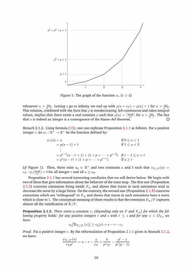
Figure 1: The graph of the function ψr (r ≥ 4)

whenever u > eFp−1 . Letting s go to infinity, we end up with ρ(u + eF ) = ρ(u) + 1 for u > eF

p−1 .

This relation, combined with the facts that ρ is nondecreasing, left-continuous and takes integral

values, implies that there exists a real constant a such that ρ(u) = ⌈u−aeF⌉ for u > eF

p−1 . The fact

that a is indeed an integer is a consequence of the Hasse–Arf theorem.

Remark 2.1.2. Using formula (15), one can rephrase Proposition 2.1.1 as follows. For a positive

integer r, let ψr : R+ → R+ be the function defined by:

ψr(u) = u if 0 ≤ u < 1= p(u− 1) + 1 if 1 ≤ u < 2

...

= pr−1(u− r + 1) + (1 + p+ · · · + pr−2) if r − 1 ≤ u < r= pr(u− r) + (1 + p+ · · ·+ pr−1) if u ≥ r

(cf Figure 1). Then, there exist u0 ∈ R+ and two constants a and b such that ψFr/F (u) =eF · ψr(u−aeF

) + b for all integer r and all u ≥ u0.Proposition 2.1.1 has several interesting corollaries that we will derive below. We begin with

two of them that give information about the behavior of the trace map. The first one (Proposition

2.1.3) concerns extensions living inside F∞ and shows that traces in such extensions tend to

decrease the norm by a large factor. On the contrary, the second one (Proposition 2.1.5) concerns

extensions which are “orthogonal” to F∞ and shows that traces in such extensions have a norm

which is close to 1. The conceptual meaning of these results is that the extension F∞/F captures

almost all the ramification of K/F .

Proposition 2.1.3. There exists a constant c1 (depending only on F and F∞) for which the fol-

lowing property holds: for any positive integers r and s with r ≤ s and for any x ∈ OFs , we

have:

vp(

TrFs/Fr(x))

≥ vp(x) + s− r − c1.

Proof. Fix a positive integer r. By the reformulation of Proposition 2.1.1 given in Remark 2.1.2,

we have:ψFr/F (u)

eF pr= u− r − a

eF+

b

preF− pr − 1

pr(p− 1)

16

when u is sufficiently large. Thanks to formula (16), we find:

vp(DFr/F ) = r +a

eF− b

preF+

pr − 1

pr(p− 1).

Given now two integers r and s with r ≤ s, the transitivity property of the different implies that:

vp(DFs/Fr) = vp(DFs/F )− vp(DFr/F ) = s− r − b

pseF+

b

preF+

ps − 1

ps(p− 1)− pr − 1

ps(p − 1).

Then there exists c ∈ N, not depending on r and s, such that vp(DFs/Fr) ≥ s − r − c. Going

back to the definition of the different, we obtain the inclusion TrFs/Fr(pr−s+cOFs) ⊂ OFr . Let

now x ∈ Fs and let v be the integer part of vp(x). Then p−vx falls in OFs , so that we get

TrFs/Fr(pr−s+c−vx) ∈ OFr , i.e. TrFs/Fr

(x) ∈ ps−r−c+vOFr . Consequently:

vp(TrFs/Fr(x)) ≥ s− r − c+ v ≥ vp(x) + s− r − c− 1.

We can then take c1 = c+ 1.

Remark 2.1.4. For a fixed integer r, we can glue the TrKs/Kr(for s varying) and define a function

Rr : K∞ → Kr by Rr(x) = pr−s TrKs/Kr(x) for x ∈ Ks. We notice that the above definition

makes sense because if s ≤ t, the functions pr−s TrKs/Krand pr−t TrKt/Kr

coincide on Ks.

Proposition 2.1.3 shows that the function Rr obtained this way is uniformly continuous. It then

extends (uniquely) to the completion K∞ of K∞.

The functions Rr : K∞ → Kr are called the Tate’s normalized traces.

Proposition 2.1.5. Let L be a finite Galois extension of F . For all ε > 0, there exist a positive

integer r and an element x ∈ OL·Fr such that vp(TrL·Fr/Fr(x)) ≤ ε.

Proof. Up to replacing F by F∞ ∩L, we may assume that F∞ and L are linearly disjoint over F .

We set L∞ = L·K∞ and Lr = L·Fr for all r. The extension L∞/L is then a Zp-extension and the

Lr’s correspond to the subgroups prZp.By formula (16) and Remark 2.1.2, there exist u0 ∈ R+ and a, b, a′, b′ ∈ R for which:

ψL/F (u) = eL/F ·(

u− vF (DL/F ))

ψLr/Fr(u) = eL/F ·

(

u− vFr(DLr/Fr))

ψFr/F (u) = eF · ψr(u− a

eF

)

+ b

ψLr/L(u) = eF · ψr(u− a′

eL

)

+ b′

for all u ≥ u0 and all positive integer r. Writing ψLr/L ψL/F = ψLr/Fr ψFr/F , we obtain:

eL · ψr( u

eF− a

eF

)

+ eL/F ·(

b− vFr(DLr/Fr))

= eL · ψr( u

eF−vF (DL/F )

eF− a′

eL

)

+ b′

for u ≥ u0. When r is sufficiently large, the above identity of functions implies, by comparing

slopes, that aeF

=vF (DL/F )

eF+ a′

eLand b − vFr(DLr/Fr

) = b′. From the latter equality, we derive

vp(DLr/Fr) = b−b′

eF pr.

Let πFr be a uniformizer of Fr. Let y be an element of DLr/Frwith vp(y) = b−b′

eF pr. By

definition of the different, there exists z ∈ OLr such that TrLr/Fr( zπFry

) 6∈ OFr . In other words,

vp(TrLr/Fr( zy )) <

1eF pr

. Set n = ⌈b−b′⌉ and x = πnFr

zy . We have vp(x) ≥ n−(b−b′)

eF pr≥ 0; hence

x ∈ OLr . Moreover:

vp(TrLr/Fr(x)) = vp

(

πnFrTrLr/Fr

( zy ))

=n

eF pr+ vp

(

TrLr/Fr( zy ))

<n+ 1

eF pr<b− b′ + 2

eF pr.

We conclude the proof by noticing that, when r goes to infinity, the upper bound b−b′+2eF pr

con-

verges to 0.

17

We shall also need the following result which is a refinement of the classical additive Hilbert’s

theorem 90, allowing in addition some control on the valuation.

Proposition 2.1.6. There exists a constant c2 (depending only on F and F∞) for which the

following property holds: for any positive integers r and s with r ≤ s and for any x ∈ OFs

with TrFs/Fr(x) = 0, there exists y ∈ Fs such that (i) TrFs/Fr

(y) = 0, (ii) x = γry − y and

(iii) vp(y) ≥ vp(x)− c2.Moreover y is uniquely determined by the conditions (i) and (ii).

Proof. We set d = s− r and:

y = − 1

pd·pd−1∑

i=0

i γir(x).

Noticing that γpd

r is the identity on Fs, we find that γry − y = x + 1pd

TrFs/Fr(x) = x. Moreover

the assumption on the trace of x implies that TrFs/Fr(y) vanishes as well.

Let now c1 be the constant of Proposition 2.1.3 and set c2 = c1 + 1. For m ∈ 0, . . . , d, we

define xm = 1pd−m TrFs/Fr+m

(x) and ym = − 1pm ·

∑pm−1i=0 i γir(xm). Obviously xd = x and yd = y.

Moreover, noticing that any integer between 0 and pm−1 can be uniquely written as a + pm−1bwith 0 ≤ a < pm−1 and 0 ≤ b < p, we obtain:

ym−1 − ym =1

p·pm−1−1∑

a=0

p−1∑

b=0

b γa+pm−1b

r (xm).

Therefore vp(ym) ≥ min(vp(xm)−1, vp(ym−1)) and so vp(y) = vp(yd) ≥ min1≤m≤d vp(xm)−1. By

Proposition 2.1.3, we end up with vp(y) ≥ vp(x)− c2. The element y we have constructed then

satisfies the requirements (i), (ii) and (iii).

It remains to prove unicity. Assume that we have given y1 and y2 such that TrFs/Fr(y1) =

TrFs/Fr(y2) and x = γry1 − y1 = γry2 − y2. Set z = y1 − y2. The second condition implies

that z is fixed by γr. Hence z ∈ Fr and TrFs/Fr(z) = ps−rz. On the other hand, one has

TrFs/Fr(z) = TrFs/Fr

(y1)− TrFs/Fr(y2) = 0. We conclude that ps−rz = 0 and hence y1 = y2.

Remark 2.1.7. Using Tate’s normalized traces (cf Remark 2.1.4), one may extend Proposition 2.1.6

for x ∈ K∞. The result we obtain reads as follows: for all x ∈ K∞ with Rr(x) = 0, there ex-

ists a unique y ∈ Kr such that x = γry − y and Rr(y) = 0. Moreover, this element y satisfies

vp(y) ≥ vp(x) − c2. In other terms, the function (γr − id) is bijective on the kernel of Rr and its

inverse is continuous.

2.2 Cp-admissibility

We now come to the study of Cp-admissibility of representations of GK . The main objective of

this subsection is to prove Theorem 1.4.6 whose statement is recalled below.

Theorem 2.2.1. Let V be a Qp-linear finite dimensional representation of GK . Then V is Cp-admissible if and only if the inertia subgroup of GK acts on V through a finite quotient.

As an application, in §2.2.3, we will explain how Theorem 2.2.1 can be used to understand

better the internal structure of Hodge–Tate representations.

2.2.1 Preliminaries

Before giving the proof of Theorem 2.2.1, we need some preparation. The first input that we

shall use is Ax–Sen–Tate theorem, whose purpose is to compute the fixed subspace of Cp under

the action of GK . As in the previous subsection, we shall work over a base F which is itself a

finite extension of K. For convenience, we set GF = Gal(K/F ).

18

Theorem 2.2.2 (Ax–Sen–Tate). We have CGFp = F .

We shall prove a “finite” version of Ax–Sen–Tate theorem which is more precise.

Theorem 2.2.3. There exists a constant c3 (depending only on F ) for which the following property

holds: for all real number v and all x ∈ K such that vp(gx − x) ≥ v for all g ∈ GF , there exists

z ∈ K such that vp(x− z) ≥ v − c3.

Proof. Throughout the proof, we fix a Zp-extension F∞ of F . We recall that such an extension

always exists and can be built from the cyclotomic extension of F as discussed in §1.1.2.

Let L be a finite Galois extension of Qp in which x lies. Thanks to Proposition 2.1.5, one can

choose an integer r together with an element λ ∈ L·Fr with the property that vp(TrL·Fr/Fr(λ)) ≤

1. We consider the elements:

y =TrL·Fr/Fr

(λx)

TrL·Fr/Fr(λ)

∈ Fr and z =1

pr· TrFr/F (y) ∈ F.

The fact that vp(gx− x) ≥ v for all g ∈ GF implies that vp(y − x) ≥ v − 1.

Observe that TrFr/F (y − z) = prz − prz = 0 and (γ0 − id)(y − z) = γ0y − y. In other words,

the element y − z has trace 0 and is an antecedent of γ0y − y by the application (γ0 − id). By

Proposition 2.1.6, it follows that vp(y − z) ≥ vp(γ0y − y)− c2. Now notice that the combinaison

of vp(γ0x− x) ≥ v and vp(y − x) ≥ v− 1 ensures that vp(γ0y− y) ≥ v− 1. Therefore, we obtain

vp(y − z) ≥ v− (c2 +1). Finally vp(x− z) ≥ min(vp(x− y), vp(y− z)) ≥ v− (c2 +1) and we can

take c3 = c2 + 1.

Proof of Theorem 2.2.2. Let x ∈ CGFp . We consider a positive integer n. Since Cp is the com-

pletion of Qp, one can find an element xn ∈ Qp such that vp(x − xn) ≥ n. We then have

vp(gxn−xn) ≥ n for all g ∈ GF . By Theorem 2.2.3, one can find zn ∈ K such that vp(zn−xn) ≥n− c3. This implies that vp(zn − x) ≥ n− c3 as well. The sequence (zn)n≥1 then converges to x.

Since zn ∈ K for all K, we obtain x ∈ K.

Remark 2.2.4. As presented above, it seems that the proof of Theorem 2.2.2 uses class field

theory (via Proposition 2.1.1). In fact, it is not the case because we have the choice on the Zp-extension F∞. If we decide to take the Zp-part of the cyclotomic extension, the computation of

the ramification filtration of Gal(F∞/F ) can be carried out explicitely, so that Proposition 2.1.1

can be proved in this case without making any reference to class field theory.

The proof we have exposed above is essentialy due to Tate [40]. A few years later, Ax [2]

reproves the theorem using a more direct and elementary argument. We presented Tate’s proof

because we believe that it serves as a very good introduction to the developments we will discuss

afterwards, which are all modeled on the same strategy: in order to study the action of GF (on

some space), we will always first descend to F∞ using Proposition 2.1.5 and then to F—or

possibly only Fr for some finite r—using Proposition 2.1.3 or Proposition 2.1.6.

Ax’s proof provides in addition an explicit value for the constant c3, namely p(p−1)2

. Ax asks

for the optimality of this constant. In [34], Le Borgne answers this question and shows that the

optimal constant is not p(p−1)2

, but 1p−1 . Le Borgne’s proof follows Tate’s strategy but uses a non

Galois extension in place of the cyclotomic extension.

An extension of Hilbert’s theorem 90. Another input we shall need is a variant of Hilbert’s

theorem 90 (cf Theorem 1.3.3) valid for infinite unramified extensions. We recall that Kur

denotes the maximal unramified extension of K (inside K). We define Kur as the completion of

Kur; it is a field which naturally embeds into Cp and which is equipped with a canonical action

of Gal(Kur/K).

Proposition 2.2.5. Any finite dimensional Kur-semi-linear representation of Gal(Kur/K) is trivial.

19

Remark 2.2.6. Proposition 2.2.5 implies in particular that unramified representation of GK are

Kur-admissible and then a fortiori Cp-admissible. It then appears as a first step towards the

proof of Theorem 2.2.1.

Proof of Proposition 2.2.5. In order to simplify notations, we denote by O the ring of integers of

Kur, and by m its maximal ideal. We recall that the quotient O/m is isomorphic to an algebraic

closure k of k. We recall also that Gal(Kur/K) is a procyclic group generated by the Frobenius

Frobq : x 7→ xq (where q is the cardinality of k).

Let W be a finite dimensional Kur-semi-linear representation. We fix (v1,0, . . . , vd,0) a basis

of W over Kur. Let OW be a O-span of v1,0, . . . , vd,0. We are going to construct a sequence of

tuples (v1,n, . . . , vd,n) such that vi,n+1 ≡ vi,n (mod mn) and Frobq(vi,n) ≡ vi,n (mod mn) for all

i ∈ 1, . . . , d and all n ∈ N.

We proceed by induction on n. The case n = 1 reduces to the fact that OW /mOW is trivial

as a k-semi-linear representation of Gal(Kur/K) ≃ Gal(k/k). In order to prove this, we remark

that, using continuity, OW /mOW descends at finite level: there exist a finite extension ℓ of kand a ℓ-semi-linear representation Wℓ of Gal(ℓ/k) such that k⊗ℓWℓ = OW /mOW . The property

we want to establish then follows from Hilbert’s theorem 90 (cf Theorem 1.3.3).

We now assume that (v1,n, . . . , vd,n) has been constructed. We look for vectors w1, . . . , wn ∈OW such that Frobq(vi,n + πnwi) ≡ vi,n + πnwi (mod mn+1) for all i. Letting wi be the image of

wi in OW /mOW , the system we have to solve can be rewritten Frobqwi − wi = ci (1 ≤ i ≤ d)

where ci is defined as the image ofFrobqvi,n−vin

πn in OW /mOW . It is then enough to prove that

(Frobq− id) is surjective on OW/mOW . This follows directly from the triviality of OW /mOW and

the fact that (Frobq − id) is surjective on k.

We conclude the proof by remarking that, for any fixed i, the sequence vi,n is Cauchy and

hence converges to a vector vi ∈ OW on which Gal(Kur/K) acts trivially. Moreover the family

of vi’s is an O-basis of OW (because its reduction modulo m is a basis of OW /mOW ) and then it

is also a Kur-basis of W .

2.2.2 Proof of Theorem 2.2.1

We are now ready to prove Theorem 2.2.1.

Write d = dimQp V . We first assume that the inertia subgroup acts on V through a finite quo-

tient. In other words, there exists a finite extension L ofKur for which Gal(K/L) acts trivially on

V . By Hilbert’s theorem 90 (cf Theorem 1.3.3), the L-semi-linear representation L⊗Qp V admits

an L-basis (v1, . . . , vd) on which the action of Gal(L/Kur) is trivial. Consequently Gal(Kur/K)operates on the Kur-span of v1, . . . , vd. By Proposition 2.2.5, this semi-linear representation is

trivial. Therefore V is (L·Kur)-admissible. It is then also Cp-admissible.

We now focus on the converse. We assume that V is Cp-admissible. Then by definition, there

exists a Cp-basis (w1, . . . , wd) of Cp ⊗Qp V with the property that gwi = wi for all g ∈ GK and

all i ∈ 1, . . . , d. Let (v1, . . . , vd) be a basis of V over Qp and let P ∈ GLd(Cp) be the matrix

representating the change of basis between the vi’s and the wi’s. Up to rescaling the vi’s, we may

assume without loss of generality that P ∈Md(OCp).From the fact that the Qp-span of the vi’s is stable under the action of GK , we derive that

the matrix Ug = P−1 · gP has coefficients in Qp for all g ∈ GK . Let c3 be the constant of

Theorem 2.2.3 and let v be a positive integer for which pv·P−1 has coefficients in OCp . By

continuity of the action of GK , denoting by Id the identity matrix of size d, there exists an open

subgroup H of GK such that vp(Ug − Id) ≥ v+ c3 +1 for all g ∈ H. Multiplying by P on the left,

we get vp(P − gP ) ≥ v + c3 + 1 for all g ∈ H. Applying now Theorem 2.2.3 (to each entry of

P ), we find a matrix P0 ∈ GLn(L) such that P ≡ P0 (mod pv+1). multiplying by P−1 on the left,

we get P−1P0 ≡ Id (mod p). Define M = P−1P0. Writing P = P0M−1, we find M · gM−1 = Ug

for all g ∈ H. Since M ≡ Id (mod p), the matrix N = logM is well defined and satisfies the

relation N − gN = logUg for all g ∈ H.

20

Let F be the extension of K cut out by H. We are going to prove that H ∩ IK operates

trivially on N . Let ξ be an entry of N . The relation N − gN = logUg ensures that ξ − gξ ∈ Zpwhenever g is in H. Define the function α : H → Zp by α(g) = gξ − ξ. The computation

α(g1g2) = g1g2ξ − ξ = g1(g2ξ − ξ) + (g1ξ − ξ) = (g2ξ − ξ) + (g1ξ − ξ) = α(g2) + α(g1)

shows that α is an additive character. Its kernel defines a Galois extension F∞ of F whose Galois

group embeds into Zp. Moreover, by construction, H ∩ kerα acts trivially on ξ. We then need to

prove that F∞ is unramified over F .

We assume by contraction that the extension F∞/F is ramified. In particular, it is not trivial,

and hence it is a Zp-extension. Proposition 2.1.3 then applies and ensures that there exists a

constant c1 such that:

vp(TrFs/Fr(z)) ≥ vp(z) + s− r − c1 (17)

whenever s ≥ r and z ∈ Fs. Let v be a positive real number and let x be an element of K such

that vp(x − ξ) ≥ v. From the equality gξ − ξ = α(g), we derive vp(

gx − x − α(g))

≥ v for all

g ∈ H. In particular, if g ∈ H ∩ kerα, we obtain vp(gx − x) ≥ v. By continuity, this estimation

is also correct for g ∈ Gal(K/Fs) for some integer s. Repeating the first part of the proof of

Theorem 2.2.3 (with the Zp-extension F∞/F ) and possibly enlarging s, we find that there exists

y ∈ Fs with the property that vp(x− y) ≥ v − 1. Thus vp(ξ − y) ≥ v − 1 as well.

Fix now g ∈ H and set z = gy − y − α(g). By our assumption on ξ, we know that vp(z) ≥v − 1. Using (17) with r = 0, we obtain vp(TrFs/F0

(z)) ≥ v + s − c1. On the other hand,

a direct computations yields TrFs/F0(z) = −psα(g). Combining these two inputs, we deduce

vp(α(g)) ≥ v − c1. Since this estimation holds for all g ∈ H and all v ∈ R+, we end up with

α = 0. This means that F∞ = F and then contradicts our assumption that F∞/F was ramified.

Remark 2.2.7. It follows from the proof above (cf in particular the first paragraph of the proof)

that a representation is Cp-admissible if and only if it is (L·Kur)-admissible for a finite extension

L of Kur. We will reuse this property in §4.2 when we will compare Cp-representations with de

Rham representations.

2.2.3 Application to Hodge–Tate representations

Beyond its obvious own interest, Theorem 2.2.1 can be thought of as a first result towards the

study of Hodge–Tate representations. Recall that a finite dimensional Qp-linear representation

V of GK is Hodge–Tate if Cp ⊗Qp V decomposes as:

Cp ⊗Qp V = Cp(χn1

cycl)⊕ Cp(χ

n2

cycl)⊕ · · · ⊕ Cp(χ

nd

cycl) (18)

for some integers ni’s. Theorem 2.2.1 implies the following unicity result.

Proposition 2.2.8. Let V be a finite dimensional Hodge–Tate representation of GK . Then the

integers ni of Eq. (18) are uniquely determined up to permutation.

Proof. We have to show that, if Cp(χn1

cycl) ⊕ · · · ⊕ Cp(χ

nd

cycl) ≃ Cp(χ

m1

cycl) ⊕ · · · ⊕ Cp(χ

md′

cycl), then

d = d′ and the ni’s agree with the mi’s up to permutation. For this, it is enough to check that,

given two integers n and m,

HomRepCp(GK )

(

Cp(χncycl),Cp(χ

mcycl)

)

(19)

is a one dimensional K-vector space if n = m, and is zero otherwise.

Let W = HomCp

(

Cp(χncycl),Cp(χ

mcycl)

)

≃ Cp(χn−mcycl

) (equipped with its Galois action). The

space (19) is equal to WGK . When n = m, it is then CGKp which is indeed equal to K by Ax–Sen–

Tate theorem (cf Theorem 2.2.2). If n 6= m, we need to prove that W is not trivial, which means

that the representation V = Qp(χn−mcycl

) is not Cp-admissible. By Theorem 2.2.1, we are reduced

21

to justify that the inertia subgroup of Qp does not act on V through a finite quotient. This is

clear because the extension cut out by the kernel of χn−mcycl

is the p-adic cyclotomic extension

which is infinitely ramified.

Remark 2.2.9. A byproduct of the proof above is that the Cp-semi-linear representation Cp(χncycl)

has no nonzero invariant vector when n 6= 0. We will reuse repeatedly this property in the

sequel.

Example 2.2.10. Recall that, assuming p > 2, we have classified the characters of GQp in Propo-

sition 1.1.1: they are all of the form µλ · χacycl · ωbcycl with a ∈ Zp and b ∈ Z/(p−1)Z. Here µλdenotes the unramified character taking the Frobenius Frobq to λ and ωcycl = [χcycl modp]. Since

the representations Cp(µλ) and Cp(ωbcycl) are Cp-admissible, we obtain:

Cp(µλ · χacycl · ωbcycl) ≃ Cp(χacycl).

Hence the character µλ ·χacycl ·ωbcycl is Hodge–Tate if and only if a ∈ Z. In this case, its Hodge–Tate

weight is a.

Example 2.2.11. Let α : GK → Zp be an additive character, e.g. α = logχcycl. Consider the two

dimensional representation V corresponding to the group homomorphism:

GK → GL2(Qp), g 7→(

1 α(g)0 1

)

.

In order terms, V = Q2p and GK acts to V by g ·(u, v) = (u, v+α(g)u). We have an obvious exact

sequence 0→ Qp → V → Qp → 0 where the action of GK on the two copies of Qp is the trivial

action. Tensoring this sequence by Cp, we get 0 → Cp → V → Cp → 0. The representation

V is Hodge–Tate if and only if the above sequence splits, if and only if V is Cp-admissible. By

Theorem 2.2.1, this happens if and only if α(IK) is finite (where IK is the inertia subgroup

of GK). Since α(IK) is a subgroup of Zp, the previous condition is equivalent to the fact that

α(IK) is reduced to 0. As a conclusion, the representation V is Hodge–Tate if and only if α is

unramified. In this case, the Hodge–Tate weights of V are 0 with multiplicity 2.

Hodge–Tate representations and admissibility. It is important to notice that the class of

Hodge–Tate representations fits very well in Fontaine’s framework presented in §1.4. Precisely,

let us consider the rings BHT = Cp[t, t−1] and B′

HT = Cp((t)). We equip them with the Galois

action obtained by letting GK act naturally on Cp and act on t by gt = χcycl(g) t for all g ∈ GK .

In addition, we define a filtration of B′HT by FilmB′

HT = tmCp[[t]] for m varying in Z. The graded

ring of B′HT is, by definition:

grB′HT =

⊕

m∈Z

FilmB′HT/FilmB′

HT.

We observe that it is canonically isomorphic to BHT. Besides, we have a natural GK -equivariant

inclusion BHT → B′HT. Ax–Sen–Tate theorem, together with the fact that Cp(χ

ncycl) has no

nonzero invariant vectors as soon as n 6= 0, implies that (BHT)GK = (B′

HT)GK = K.

Proposition 2.2.12. The rings BHT and B′HT satisfy Fontaine’s assumptions (H1), (H2) and (H3)

(introduced in §1.4.1).

Proof. This is obvious for B′HT since it is a field. As for BHT, it is clearly a domain. Moreover

since B′HT is a field, we have BHT ⊂ Frac BHT ⊂ B′

HT. Taking the GK -invariants, we obtain

(Frac BHT)GK = K; hence BHT satisfies (H2). Finally, we prove that BHT satisfies (H3). Let

x ∈ BHT, x 6= 0 and assume that the line Qpx is stable by GK . We have to prove that x is

invertible in BHT. Up to multiplying x by some power of t, we may assume that x ∈ Cp[t]. Write

22

x = a0 + a1t + · · · + antn where the ai’s are in Cp. Our assumption implies that there exists

λ ∈ Qp such that gai · χ(g)i = λai for all g ∈ GK and all i ∈ 0, 1, . . . , n. Let j be an index for

which aj 6= 0 and write µi =aiaj

for all i. We then have gµi = χ(g)j−iµi for all g and i. If i 6= j,

this implies that µi = 0 since Cp(χj−icycl

)GK = 0. Therefore x has to be equal to ajtj, and so is

invertible in BHT.

Proposition 2.2.13. Let V be a finite dimensional Qp-linear representation. Then V is Hodge–Tate

if and only if it is BHT-admissible, if and only if it is B′HT-admissible.

Proof. Write d = dimQp V . Observe that BHT =⊕

m∈Z Cp(χmcycl) as a Cp-semi-linear representa-

tion. Therefore:(

V ⊗Qp BHT

)GK ≃⊕

m∈Z

(

V ⊗ Cp(χmcycl)

)GK .

Suppose that V is Hodge–Tate. Let m1, . . . ,ms be its Hodge–Tate weights and e1, . . . , es be the

corresponding multiplicities. The space(

V ⊗ Cp(χ−mi

cycl))GK has then dimension ei. Summing

up all these contributions, we find that (V ⊗Qp BHT)GK has dimension d, which means that V is

BHT-admissible.

The converse and the case of B′HT are proved in a similar fashion and left to the reader.

2.3 Complement: Sen’s theory

The aim of this subsection is to expose Sen’s theory [35] whose objective is to provide a sys-

tematic study of finite dimensional Cp-semi-linear representations of GK . In what follows, we

choose and fix once for all a Zp-extension K∞ of K. We let α : Gal(K∞/K) → Zp be the at-

tached group isomorphism. As in §2.1.2, we put γr = α−1(pr) and let Kr be the subextension of

K∞ corresponding to the closed subgroup α−1(prZp).We recall that one possible choice is α = log χcycl, in which case K∞ is the Zp-part of the

cyclotomic extension of K (cf §1.1.2). Actually, strictly speaking, Sen’s theory only concerns this

particular choice of α. However the extension of general α’s is straightforward. In what follows,

we do not restrict ourselves to α = logχcycl.

Remark 2.3.1. Recently, Berger and Colmez [4] generalized Sen’s theory, allowing α to take its

values in any p-adic Lie group (possibly noncommutative). Their theory relies on the notion of

locally analytic vectors, which is not needed in classical Sen’s theory (finite vectors are enough

as we shall explain below). We will not expose their generalization in the article and do restrict

ourselves to homomorphisms α taking their values in Zp.

We recall that, given a topological group G and a topological ring B on which G acts, we

have introduced the notation RepB(G) for the category of B-semi-linear representations of G.

Let RepfB(G) denote the full subcategory of RepB(G) consisting of representations which are

finitely generated as a B-module. When B is the field, RepfB(G) is then the category of finite

dimensional B-semi-linear representations of G.

Descend. The first result towards Sen’s theory is Proposition 2.3.2 just below, which could

understood as an analogue of Hilbert’s theorem 90 for the Galois group Gal(K/K∞).

Proposition 2.3.2. Let W ∈ RepfCp(GK). Then there exist an integer r and a Cp-basis v1, . . . , vd

of W such that gvi = vi for all g ∈ Gal(K/K∞).

Proof. The proof is similar to that of Proposition 2.2.5.

Let OW be any OCp -lattice in W . As a first step, we are going to construct a Cp-basis

w1, . . . , wd of W with wi ∈ OW , gwi ≡ wi (mod p2OW ) for all g ∈ Gal(K/K∞) and pOW ⊂OCpw1 ⊕ · · · ⊕ OCpwd. By continuity of the Galois action, there exists a finite Galois extension

23

L of K such that gw ≡ w (mod p2OW ) for all g ∈ Gal(K/L) and all w ∈ W . For a positive

integer r, set Lr = L·Kr. By the proof of Proposition 2.1.3, we know that there exists r for

which vp(DLr/Kr) < e−1

L/K . We fix such an r.

Let λ1, . . . , λm be a OKr -basis of OLr and let g1, . . . , gm be the elements of Gal(Lr/Kr). For

i ∈ 1, . . . ,m, choose gi ∈ GK a lift of gi. We define the elements:

yi,j =m∑

i′=1

gi′(λjxi) =m∑

i′=1

gi′(λj) · gi′(xi)

for i varying between 1 and d and j varying between 1 and m. It is easily seen that gyi,j ≡ yi,j(mod p2OW ) for all g ∈ Gal(K/Kr). Moreover, the determinant of the matrix (gi(λj))1≤i,j≤m is,

by definition, the discriminant of Lr/Kr. Its p-adic valuation is then less than 1 thanks to our

assumption on vp(DLr/Kr). We deduce that there exist µ1, . . . , µm ∈ OLr with the property that

∑mj=1 µjTrLr/Kr

(λj) = p. Hence∑m

j=1 µjyi,j ≡ pxi (mod p2OW ) for all i. The OCp -span of the

yi,j ’s then contains pOW . Among these vectors, one can select d of them w1, . . . , wd whose span

still contains pOW . The wi’s satisfy all the announced properties.

The second step of the proof consists in lifting the wi’s by a process of successive approxima-

tions. In order to simplify the notations, we redefine OW as the OCp -span of w1, . . . , wd. With

the new definition, we have gwi ≡ wi (mod pOW ) for all g ∈ Gal(K/K∞). We will construct by

induction on n a sequence of families (v1,n, . . . , vd,n) satisfying the following congruences:

vi,n+1 ≡ vi,n (mod pnOW ) and gvi,n ≡ vi,n (mod pnOW )

for all i ∈ 1, . . . , d, n ∈ N and g ∈ Gal(K/K∞). For n = 1, we set vi,1 = wi. Now we assume

that the vi,n’s have been constructed. By continuity there exists a finite Galois extension L of Ksuch that gvi,n ≡ vi,n (mod pn+2OW ) for all g ∈ Gal(K/L). By Proposition 2.1.3, there exist an

integer r and λ ∈ OLr (with Lr = L·Kr) such that vp(TrLr/Kr(λ)) ≤ 1. As in the first step, we

let g1, . . . , gm be the elements of Gal(Lr/Kr) and we choose a lifting gi ∈ GK of gi. We define:

vi,n+1 =1

TrLr/Kr(λ)·m∑

j=1

gj(λvi,n) =1

TrLr/Kr(λ)·m∑

j=1

gj(λ) · gj(vi,n)

and check that the vi,n+1’s satisfy the desired requirements.

We conclude the proof by taking the limit with respect to n.

Proposition 2.3.2 tells us that the W is trivial when viewed as a Cp-linear representation of

Gal(K/K∞). Moreover by the proof of Ax–Sen–Tate theorem, the fixed field CGal(K/K∞)p is the

completion ofK∞, that we shall call K∞. By general results of trivial semi-linear representations

(cf §1.3.2), we then have an isomorphism

Cp ⊗K∞

WGal(K/K∞) ≃W

for all Cp-semi-linear representation of W . We notice that WGal(K/K∞) inherits an action of

Gal(K∞/K).

Finite vectors. Set Γ = Gal(K∞/K). The second step is Sen’s theory is the study of K∞-

semi-linear representations of Γ. To this attempt, Sen defines the subspace of finite vectors as

follows.

Definition 2.3.3. Let W ∈ RepfK∞

(Γ). A vector v ∈ W is finite if the K∞-subspace of W

generated by the gv for g varying in Γ is finite dimensional over K∞.

As an example, the subspace of finite vectors of the semi-linear representation K∞ itself is

K∞. In general, one easily checks that the subspace of finite vectors is a vector space over K∞.

24

Proposition 2.3.4. Let W ∈ RepfK∞

(Γ). Then, there exist an integer r and a basis (v1, . . . , vd) of

W with the property that the Kr-span of the vi’s is stable under the Γ-action.

Remark 2.3.5. Obviously, the vi’s of Proposition 2.3.4 are finite in the sense of Definition 2.3.3.

Therefore, we deduce that the subspace of finite vectors ofW generatesW as a K∞-vector space.

Finite vectors are then numerous.

Proof of Proposition 2.3.4. Let c2 be the constant of Proposition 2.1.6. It is harmless to assume

that c2 is an integer. To simplify notation, we write L = K∞. Let OL be the ring of integers of L.

We choose a OL-lattice OW inside W . By continuity, there exists an integer r such that gw ≡ w(mod pc2+1OW ) for all g ∈ Gal(K∞/Kr) and all w ∈W . We choose and fix such an r. The group

Gal(K∞/Kr) acts on OW and on all the quotients OW /pnOW for n ∈ N.

We are going to construct, by induction of n, a sequence of families (v1,n, . . . , vd,n)n≥1 of

elements of OW with the following properties:

(i) for all n, the family v1,n, . . . , vd,n is an OL-basis of OW ,

(ii) for all n ≥ 1 and all i, vi,n+1 ≡ vi,n (mod pnOW )

(iii) the OKr -submodule of OW /pn+c2OW generated by the classes of the vi,n’s (1 ≤ i ≤ d) is

stable under the Gal(K∞/Kr)-action.

For n = 1, we pick an arbitrary OL-basis v1,1, . . . , vd,1 of OW . Since Gal(K∞/Kr) acts trivially on

OW/pc2+1OW , all the requirements are fulfilled. We now assume that v1,n, . . . , vd,n have been

constructed. By the induction hypothesis, for all i, we can write γrvi,n = vi,n +∑d

j=1(λi,j +εi,j)vj,n where the λi,j ’s lie in Kr and the εi,j ’s have p-adic valuation at least n + c2. Moreover,

since the action of γr is trivial modulo pc2+1, we deduce vp(λi,j) ≥ c2+1. Let Rr : L→ Kr be the

Tate’s normalized trace defined in Remark 2.1.4. By Proposition 2.1.6 (cf also Remark 2.1.7),

for all i and j, there exists µi,j ∈ L with vp(µi,j) ≥ n and εi,j = Rr(εi,j) + γrµi,j − µi,j. For all

i, define vi,n+1 = vi,n −∑d

j=1 µi,jvj,n. Since the µi,j ’s have all valuation at least n, the items (i)

and (ii) are fulfilled. Besides, a simple computation gives:

γrvi,n+1 = vi,n+1 +

d∑

j=1

(

λi,j +Rr(εi,j))

· vj,n +d∑

j=1

γrµi,j ·(

vj,n − γrvj,n)

.

Since γr acts trivially modulo pc2+1, the last summand lies in pn+c2+1OW . Noting in addition that

vj,n ≡ vj,n+1 (mod pnOW ) and that the λi,j ’s are all divisible by pc2+1, we obtain the congruence:

γrvi,n+1 ≡ vi,n+1 +d∑

j=1

(

λi,j +Rr(εi,j))

· vj,n+1 (mod pn+c2+1OW )

from which the item (iii) follows.

Passing to the limit, we obtain an L-basis v1, . . . , vd of W whose Kr-span is stable under the

action of Gal(Kr/K). It remains to prove that it is stable under the whole action of Γ. Let M0

and Mr be the matrices that gives the action of γ0 and γr on L respectively, that are:

(γ0v1 · · · γ0vd) = (v1 · · · vd) ·M0

(γrv1 · · · γrvd) = (v1 · · · vd) ·Mr.

We do know that Mr has all its entries in Kr and we want to prove that the same holds for M0.

Actually, from our construction of the vi’s, we know further that Mr has integral entries and that

it is congruent to the identity matrix modulo pc2+1. From the commutation of γ0 and γr, we

derive the relation M0 · γ0Mr = Mr · γrM0. Define C = Rr(Mr) −Mr where Rr is the Tate’s

normalized trace. We want to prove that C vanishes.

25

Since Rr commutes with γr, we have the relation C ·γ0Mr =Mr ·γrC, from which we derive

γrC − C = M−1r · C · γ0Mr. Set N = M−1

r · C · γ0Mr and let v be the smallest valuation of

an entry of C. We assume by contradiction that v is finite. The fact that Mr ≡ Id (mod pc2+1)implies that N is divisible by pv+c2+1. By unicity in Proposition 2.1.6 (and Remark 2.1.7), we

deduce that C must be divisible by pv+1. This contradicts the definition of v.

Sen’s operator. We now put together the results we have established before. LetW ∈ RepfCp(GK).

We define W∞ = WGal(K/K∞) and let W∞ be the subspace of finite vectors of W∞. Combining

Propositions 2.3.2 and 2.3.4, we find that W admits a Cp-basis consisting of elements of W∞. In

other words, the canonical mapping Cp⊗K∞W∞ → W is an isomorphism. The action of GK on

W is then entirely determined by the action of Γ of W∞. Using the particularly simple structure

of Γ, it is possible to describe its action even more concretely.

More precisely, we consider an integer r and a basis v1, . . . , vd of W∞ such that the Kr-vector

space Wr = Krv1⊕ · · · ⊕Krvd is stable under the action of Γ (or equivalently, GK). For g ∈ GK ,

we shall denote by ρW (g) the endomorphism of Wr given by the action of g. Note that ρW (g)is Kr-linear as soon as g ∈ Gal(K/Kr). In particular ρW (γs) is linear whenever s ≥ r. Since

γs converges to the identity in Γ, the logarithm of ρW (γs) is well defined for s sufficiently large.

Moreover, we have the relation p · log ρW (γs+1) = log ρW (γs) as soon as the logarithm ρW (γs) is

defined. The sequence p−s log ρW (γs) is then ultimately constant. Sen’s operator ΦW is defined

as the limit of this sequence:

ΦW = lims→∞

log ρW (γs)

ps.

We extend ΦW to W∞ by K∞-linearity. This extension is canonical in the sense that it does

not depend on the choice of r. Besides, the exponential map can be used to reconstruct the

representation W we started with, at least on a finite index subgroup of G. Precisely, there

exists an integer s such that:

ρ(g) = exp(

α(g)ΦW)

for all g ∈ Gal(K/Ks) (20)

where we recall that α : GK → Zp was the character defining the isomorphism between

Gal(K∞/K) and Zp. From (20), it follows that the action of Gal(K/Ks) on W can be entirely

reconstructed by extending the ρ(g)’s to W using semi-linearity.

Example 2.3.6. Consider the representation V given by:

GK → GL2(Qp), g 7→(

1 α(g)0 1

)

already discussed in Example 2.2.11. Set W = Cp⊗Qp V . It is easily checked that WGal(K/K∞) =

K2∞ and its subspace of finite vectors is K2

∞. Sen’s operator ΦV is the nilpotent linear morphism

(x, y) 7→ (y, 0).

Sen’s operator exhibits very interesting properties. Below, we state the most important ones.

Proposition 2.3.7. We keep the above notations. Sen’s operator ΦW is defined over K, in the sense

that W∞ admits a basis in which the matrix of ΦW has coefficients in K.

Proof. This follows from the fact that ΦW commutes with the action of Γ.

Let Sen(K,K∞) denote the category of finite dimensional K∞-vector spaces equipped with

an endomorphism defined over K (in the sense of Proposition 2.3.7). The construction W 7→(W∞,ΦW ) defines a functor S : Repf

Cp(GK) → Sen(K,K∞). Indeed a morphism f : W → W ′

in the category RepfCp(GK) necessarily maps W∞ to W ′

∞ and commutes with Sen’s operators

26

on both sides because it commutes with the Galois action. The functor S commutes with direct

sums, while its behavior under tensor products is governed by the Leibniz rule:

(W ⊗W ′)∞ =W∞ ⊗W ′∞

ΦW⊗W ′ = ΦW ⊗ idW ′ + idW ⊗ ΦW ′.

Moreover, the functor S is faithful. Indeed, assume that we are given W,W ′ ∈ RepfCp(GK),

together with a morphism f : W →W ′ such that S(f) = 0. Then, by assumption, f vanishes on

the subspace W∞. Since the latter generates W as a Cp-vector spaces, one must have f = 0. In

general, S is not full. However, it detects isomorphisms as shown by the next proposition.

Proposition 2.3.8. Let W,W ′ ∈ RepfCp(GK). We assume that S(W ) and S(W ′) are isomorphic in

Sen(K,K∞). Then W and W ′ are isomorphic in RepfCp(GK).

Proof. Let f : W∞ → W ′∞ be an isomorphism commuting with Sen’s operators. By Cp-linearity,

f extends to an isomorphism of Cp-vector spaces f : W → W ′. Moreover, thanks to formula

(20), there exists an integer s such that f is Gal(K/Ks)-equivariant.

Let V be the space of Gal(K/Ks)-equivariant Cp-linear morphisms from W to W ′. It is

endowed with a canonical action of Gal(Ks/K) and thus appears as an object in the category

RepfKs

(Gal(Ks/K)). By Hilbert’s theorem 90 (cf Theorem 1.3.3), V admits a basis (f1, . . . , fm)of fixed vectors. In other words the fi’s are GK -equivariant morphisms W → W ′. It remains

to prove that a suitable K-linear combination of the fi’s is invertible. For this, we consider the

m-variate polynomial defined by:

P (t1, t2, . . . , tm) = det(t1f1 + t2f2 + · · ·+ tmfm).

We know that P is not the zero polynomial because the Ks-span of the fi’s contains an isomor-

phism (namely f). Since K is an infinite field, P cannot vanish everywhere on Km. Hence there

exist t1, . . . , tm ∈ K such that t1f1 + · · ·+ tmfm is an isomorphism.

Corollary 2.3.9. A representation W ∈ RepfCp(GK) is trivial if and only if Sen’s operation ΦW

vanishes.

Proof. It suffices to apply Proposition 2.3.8 with W ′ = CdimWp .

We conclude our exposition of Sen’s theory by noticing that Sen’s operator is closely related

to the notion of Hodge–Tate representations. Precisely, a representation V ∈ RepfQp

(GK) is

Hodge–Tate if and only if the operator ΦCp⊗QpV is semi-stable with eigenvalues in Z, these

eigenvalues being the Hodge–Tate weights of V . (Combine Examples 2.2.11 and 2.3.6 for an

illustration of this property.) Given a general W ∈ RepfCp(GK), the eigenvalues of ΦW are

sometimes called the generalized Hodge–Tate weights of W .

3 Two refined period rings: Bcrys and BdR

Previously, we have studied the period rings Cp and BHT and discussed the attached notion of

Hodge–Tate representations. In the present section, we introduce two new period rings, called

Bcrys and BdR. As we shall see in §4, these rings have a deeper arithmetical and geometrical

content that Cp and BHT.

The definition of Bcrys and BdR is a bit elaborated and occupies all this section. In order to

ease the task of the reader, we devote two short paragraphs below to collect the most important

properties of Bcrys and BdR and sketch the main steps of their construction.

Before this, we need to recall and introduce some notations. Throughout this section, Kwill continue to refer to a finite extension of Qp. Its ring of integers (resp. its residuel field) is

27

denoted by OK (resp. k). We define K0 = W (k)[1p ]; it is the maximal unramified extension of

Qp included in K. We fix an algebraic closure K of K and set GK = Gal(K/K). Observe that

K is also an algebraic closure of Qp and hence does not depend on K. We let Kur0 (resp. Kur)

be the maximal unramified extension of K0 (resp. of K) inside K. Since K0 is unramified over

Qp, Kur0 is also the maximal extension of Qp inside K and thus is also independent of K. We let

also Cp denote the p-adic completion of K. Finally, we choose and fix once for all a uniformizer

π of K.

Main properties of Bcrys and BdR. As discussed in §1.2, the original idea behind the definition

of Bcrys is the wish to design a variant of Barsotti-type spaces (the B of §1.2) which includes the

tannakian formalism. On the geometric side, a nice tannakian framework in which p-divisible

groups naturally arise is crystalline cohomology. Indeed, in many contexts, crystalline coho-

mology provides powerful invariants that can be used to classify p-divisible groups (and more

generally finite flat group schemes) [7]. We then expect the ring Bcrys to have some “crys-

talline nature” and to be eventually related to crystalline cohomology. Apart from this, recall

that another motivation of p-adic Hodge theory is to compare etale cohomology with de Rham

cohomology. The period ring making the comparison possible—namely BdR—then needs to be

deeply related to de Rham cohomology. The algebraic structure of Bcrys and BdR is guided by

the above general expectations: the ring Bcrys (resp. BdR) will carry, as much as possible, the

same structures and exhibit similar properties as the crystalline (resp. de Rham) cohomology.

Below, we list the main features of Bcrys and BdR and, when it is possible, we make the

parallel with the corresponding properties of the cohomology. We start with BdR:

• BdR is a discrete valuation field with residue field Cp;

• BdR is an algebra over K·Kur, but not over Cp (with a defining morphism preserving the

Galois action);

• BdR is equipped with a filtration FilmBdR (which is nothing but the canonical filtration

given by the valuation); this filtration corresponds to the de Rham filtration on the coho-

mology;

• BdR has a distinguished element t on which Galois acts by multiplication by the cyclotomic

character; moreover t is a uniformizer of BdR, so that FilmBdR = tmBdR;

• the graded ring of BdR is BHT = Cp[t, t−1];

• (BdR)GK = K; this property corresponds to the fact that the de Rham cohomology is a

vector space over K.

And now for Bcrys:

• Bcrys is an algebra over Kur0 ;

• Bcrys is equipped with a Frobenius, which is a ring homomorphism ϕ : Bcrys → Bcrys; this

structure corresponds to the action of the Frobenius on the crystalline cohomology;

• there is a canonical embedding K ⊗K0 Bcrys → BdR; this property corresponds to the

fact that the crystalline cohomology defines a canonical K0-structure inside the de Rham

cohomology (this is Hyodo–Kato isomorphism);

• the distinguished element t of BdR is in Bcrys;

• (Bcrys)GK = K0; this property corresponds to the fact that the de Rham cohomology is a

vector space over K0;

•(

Bcrys ∩ Fil0BdR

)ϕ=1= Qp (the notation “ϕ=1” means that we are taking the fixed points

under the Frobenius).

28

(µ > p−1) (1 ≤ µ ≤ p−1)

B+1

B+inf

B+µ B+

crys B+µ B+

max

B+inf,K B+

µ,K B+crys,K B+

µ,K B+max,K B+

dR

Bµ Bcrys Bµ Bmax

Bµ,K Bcrys,K Bµ,K Bmax,K BdR

Figure 2: Diagram of period rings; all arrows are injective

Sketch of the construction. The starting point of the construction of Bcrys andBdR is the intro-

duction of the rings Ainf and B+inf

= Ainf[1/p]. One may think of Ainf as the universal thickening

of OK/pOK ; it is obtained via a general process (detailed in §3.1) involving a perfectization

mecanism as a first step and Witt vectors as a second step. Beyond this purely algebraic con-

struction, it is important to notice that the ring B+inf

has a strong geometrical interpretation.

Indeed as observed first by Colmez and then by Fargues–Fontaine [17] and Scholze [38], B+inf

appears at a mixed characteristic analogue6 of the ring of bounded analytic functions on the

open unit disc. Moreover B+inf

is equipped with a Frobenius (coming from the general theory

of Witt vectors) and a distinguished geometric point, which is materalized by a surjective ring

homomorphism θ : B+inf→ Cp.

Following the crystalline formalism, we then define the ring B+crys as the completion of the

divided powers envelope of B+inf

with respect to the ideal ker θ. Unfortunately, B+crys does not

have a nice geometrical interpretation, in the sense that it is not the ring of analytic functions

on a smaller domain. In order to tackle this difficulty, we introduce (following Colmez) some

variants of B+crys. Precisely, given a real parameter µ ≥ 1, one considers the rings B+

µ ’s of

analytic functions defined over some annulus Dµ included in the open unit disc, and containing

the distinguished point θ. The B+µ ’s are closely related to B+

crys (we have inclusions in both

directions), so that it is often safe to replace the latter by the formers.

Another important feature of B+crys and the B+

µ ’s is that they contain a period of the cyclo-

tomic character, that is an element t on which GK acts by multiplication by the cyclotomic

character. Geometrically, the divisor of t is the orbit of the point θ under the action of the

Frobenius, that is the union of all point θ ϕn for n varying in Z. The presence of t in B+µ will

eventually ensure the admissibility of the representation Qp(χ−1cycl

). In order to make Qp(χcycl)

admissible as well (which is of course something we really want to have), we need t to be a unit.

So we finally define Bµ = B+µ [

1t ] and the construction of Bcrys is now complete.

As for the field BdR, it is defined as the fraction field of the completion of the local field

of B+inf

(or equivalently, B+µ ) at the special point θ. The filtration on BdR is nothing but the

canonical filtration given by the order of the zero (or the pole) at θ.The diagram presented on Figure 2 summarizes the period rings we will define in this section

and the relations between them. We see on this diagram that the B+µ ’s and the Bµ’s all have

a variant denoted by an extra index K. They are defined by extending scalars from K0 to K.

These variants are interesting because, when V is a Bµ-admissible representation, the de Rham

filtration becomes visible after extending scalars to Bµ,K , which is much smaller and sometimes

6This analogy has been placed in the framework of Huber geometry by Scholze in [38] and then takes a very

substantial meaning. However, for this article, it will be sufficient to keep in mind that elements of B+inf behave like

analytic functions over a nonarchimedian base.

29

more tractable that BdR.

3.1 Preliminaries: the ring B+inf

In this subsection, we introduce the ring B+inf

which serves as a common base upon which all the

forthcoming constructions will be built.

3.1.1 Perfectization

Let ϕ denote the Frobenius morphism x 7→ xp acting on the quotientOCp/pOCp ≃ OK/pOK and

observe that ϕ is a ring homomorphism since OCp/pOCp is annihilated by p.Let R be the limit of the projective system7:

OCp/pOCp

ϕ−→ OCp/pOCp

ϕ−→ OCp/pOCp

ϕ−→ · · · ϕ−→ OCp/pOCp

ϕ−→ · · ·

Concretely, an element of R is a sequence (ξn)n≥0 of elements of OCp/pOCp satisfying the fol-

lowing compatibility property: ξpn+1 = ξn for all n ≥ 0. Clearly, R is a ring of characteristic p.In a slight abuse of notation, we continue to write ϕ for the Frobenius acting onR. Over this

ring, it is an isomorphism, its inverse being given by the shift map (ξ0, ξ1, ξ2, . . .) 7→ (ξ1, ξ2, ξ3, . . .).We sometimes say that R is the perfectization of OCp/pOCp . Moreover R is endowed with an

action of GK coming from its natural action on OCp .

Some distinguished elements. Choose a primivite p-root of unity in OK and denote it by ε1.

Similarly, choose a p-th root of ε1 and denote it by ε2; obviously, ε2 is a primitive p2-th root

of unity. Repeating inductively this process, we construct elements ε3, ε4, . . . ∈ OK such that

εpn+1 = εn for all n. Let εn ∈ OK/pOK be the image of εn. The compabitility property ensures

that the sequence (1, ε1, ε2, . . .) defines an element in R; we shall denote it by ε. We emphasize

that ε does depend on the choice of the εn’s. However, the dependency is easy to write down

explicitely: if (ε′n)n≥0 is another compatible sequence of primitive pn-th roots of unity, one can

always find an element g ∈ GK such that ε′n = gεn = εχcycl(g)n . Hence the element of R defined

the ε′n’s is εχcycl(g). In what follows, we fix once for all an element ε as above.

In a similar fashion, we choose a compatible system (pn)n≥1 of pn-root of p, i.e. pp1 = pand ppn+1 = pn for all n ≥ 1. If pn ∈ OK/pOK is the reduction of pn modulo p, the sequence

(0, p1, p2, . . .) defines an element ofR that we will denote by p. Again, p depends on the choice

of the pn’s but we can check that another choice would finally lead to an element of the form

p·εa for some a ∈ Zp. The same construction works more generally if we start for any element

x ∈ OCp in place of p; it leads to an element x ∈ R, which is well defined up to multiplication

by εa with a ∈ Zp. Besides p, we will fix a choice of π (where we recall that π is a fixed

uniformizer of K) for future use.

Valuation. The ring R is equipped with a derivation v that we are going to define now. We

start with the following observation: if x is a nonzero element inOCp/pOCp , the p-adic valuation

of x does not depend on the lifting x of x. The valuation vp then induces a well defined function

vp : OCp/pOCp → Q ∪ +∞ where we agree that vp(0) = +∞ as usual. For ξ = (ξn)n≥0 in R,

we define:

v(ξ) = limn→∞

pnvp(ξn).

The compatibility condition ξpn+1 = ξn implies that the sequence(

pnvp(ξn))

n≥0is ultimately

constant; so the limit is well defined. The function v satisfies the following properties for

ξ, ξ′ ∈ R:7This definition is s special case of a general construction (the tilt) in the theory of perfectoid spaces [36]. We

refer to Andreatta and al. lecture [1] in this volume for an introduction to perfectoid spaces. The notations p, π

and v that we will introduce later comes from the language of perfectoid spaces.

30

(1) v(R) = Q ∪ +∞,(2) v(ξ) =∞ if and only if ξ = 0,

(3) v(ξ) = 0 if and only if ξ is invertible,

(4) v(ξ + ξ′) ≥ min(v(ξ), v(ξ′)) and equality holds if v(ξ) 6= v(ξ

′),

(5) v(ξξ′) = v(ξ) + v(ξ

′).

Combining (2) and (5), we find that R is a domain. Indeed if ξ and ξ′ are nonzero elements of

R, then v(ξ) and v(ξ′) are finite, and so v(ξξ

′) = v(ξ) + v(ξ′) is also finite. The existence

of v implies that R is a local ring with maximal ideal mR consisting of elements of positive

valuation. The residue field R/mR is canonically isomorphic to k. We observe in addition that

the projection R→ k has a canonical splitting defined by:

a 7→(

[a] mod p, [a1/p] mod p, [a1/p2] mod p, . . .

)

where the notation [·] stands for the Teichmuller representative. Besides, the valuation v equips

R with a distance, and hence a topology. The Galois action on R preserves v; in particular, it is

continuous.

An easy consequence of the existence of a valuation is the following result.

Lemma 3.1.1. The projection onto the first coordinate R → OCp/pOCp induces an isomorphism

R/pR ≃ OCp/pOCp .

Proof. Let f : R → OCp/pOCp , (ξ0, ξ1, . . .) 7→ ξ0. The surjectivity of f is a consequence of the

fact that Cp is algebraically closed. On the other hand, it is clear that the kernel of f consists

of elements ξ such that v(ξ) ≥ 1. Since v(p) = 1, we deduce that ker f is the principal ideal

generated by p. This proves the lemma.

3.1.2 Witt vectors

We set Ainf = W (R) (where W (−) stands for the Witt vectors functor) and B+inf

= Ainf[1p ]. For

x ∈ R, we let [x] denote its representative Teichmuller in Ainf. Since R is perfect, an element

of Ainf can be written uniquely as a convergent series∑

i≥0[ξi] pi with ξi ∈ R for all i. A similar

decomposition holds for elements in B+inf

: each such element x has a unique expansion of the

form∑

i≥i0[ξi] p

i (with ξi ∈ R) where i0 is a (possibly negative) integer, which depends on x.

The inclusion k → R provides by functoriality a ring morphism W (k)→ Ainf. Thus Kur0 em-

beds into B+inf

. The ring Ainf is a local ring whose maximal ideal is the kernel of the composition

Ainf → W (k) → k where the first map is induced by the projection R → k and the second map

is the reduction modulo p. Concretely, it consists of series∑

i≥0[ξi] pi for which ξ0 ∈ mR.

We set Ainf,K = OK ⊗W (k) Ainf and B+inf,K = K ⊗K0 B

+inf

. These tensors products make sense

because we saw that Ainf is an algebra over W (k). The elements of B+inf,K have a canonical

expansion of the form∑

i≥i0[ξi] π

i with i0 ∈ Z and ξi ∈ R for all i ≥ i0. Moreover Ainf,K is a

local ring and its maximal ideal consists of series as above such that ξ0 ∈ mR; its residue field is

k.

Additional structures. By definition of the Witt vectors, B+inf

carries an action of a Frobenius,

that we shall continue to call ϕ. On the above representation, it is given by the simple formula:

ϕ

(

∞∑

i=i0

[ξi] pi

)

=∞∑

i=i0

[ξpi ] pi (i0 ∈ Z, ξi ∈ R). (21)

We emphasize that ϕ does not admit a canonical extension to B+inf,K as there is no canonical

Frobenius on K.

31

The ring B+inf

is also equipped with an action of GK by functorialiy of Witt vectors. Again,

this action has a simple expression, namely:

g

(

∞∑

i=i0

[ξi] pi

)

=∞∑

i=i0

[gξi] pi (i0 ∈ Z, ξi ∈ R) (22)

for all g ∈ GK . The GK -action extends to B+inf,K by letting GK act trivially on OK .

Finally, we equip Ainf and Ainf,K with the weak topology, which is the topology defined by

the ideal (p, [p]) (or equivalently, by the ideal (p, [x]) for any element x ∈ mR). Concretely, if

xn =

∞∑

i=0

[ξi,n] pi ∈ Ainf and x =

∞∑

i=0

[ξi] pi ∈ Ainf

the sequence (xn)n≥0 converges to x if ξi,n → ξi for each fixed index i ∈ N, and a similar

property holds for Ainf,K . The topology on Ainf induces a topology on the subset p−vAinf of

B+inf

for all v. Gluing them, we obtain a topology on B+inf

=⋃

v≥0 p−vAinf. In concrete terms, a

sequence (xn)n≥0 of elements on B+inf

converges to x ∈ B+inf

if and only if there exists an integer

v such that pvxn ∈ Ainf for all n and pvxn tends to pvx in Ainf as n goes to infinity. The topology

on B+K,inf

is defined similarly.

From the above descriptions, it follows that the Frobenius acts continuously on Ainf and GKacts continuously on Ainf and Ainf,K .

Newton polygons. In [17], Fargues and Fontaine argue that elements of Ainf (resp. Ainf,K)

should be thought of as analytic functions of the variable p (resp. π); indeed, they share many

properties with bounded analytic functions on the open unit disc. Similarly, elements of B+inf

and

B+inf,K resemble to bounded analytic functions on the punctured open unit disc.

In particuler, there is a well-defined notion of Newton polygons for series in B+inf

and B+inf,K .

Precisely, if x =∑

i≥i0[ξi] p

i ∈ Ainf, its Newton polygon is defined as the convex hull in R2

of the points (i, v(ξi)) together with two points at infinity in the direction of the positive x-

axis and the direction of the positive y-axis respectively. Similarly, the Newton polygon of x =∑

i≥i0[ξi] π

i ∈ Ainf,K is the convex hull of the points ( ie , v(ξi)) and the same points at infinity.

Using that πe = up for some invertible element u ∈ OK , one easily proves that the above

definition coincides with that of Newton polygons on B+inf

when x is in B+inf

. Let NPinf(x) denote

the Newton polygon of x ∈ B+inf,K .

Fargues and Fontaine prove that Newton polygons satisfy many excepted properties. For

example, they are multiplicative in the sense that NPinf(xy) = NPinf(x)+NPinf(y) where the plus

sign on the right hand side denotes the Minkowski sum. Moreover Fargues and Fontaine prove

an analogue of the Weierstrass preparation and factorization theorems in this context, showing

that Newton polygons serve as a guide for factorization in the rings B+inf

and B+inf,K as they do

for usual analytic functions. We do not reproduce their proofs here because we will only use

Newton polygons for visualizing our forthcoming constructions, and not for proving results. In

any case, we refer to [17, §1–3] for many developments in this direction.

We conclude this discussion by examining the action of the additional structures at the level

of Newton polygons. Since GK acts on R by isometries, it follows from the formula (22) that

NPinf(gx) = NPinf(x) whenever g is in GK and x is in B+inf,K . As for Frobenius, formula (21)

shows that, for any x ∈ B+inf

, we have NPinf(ϕ(x)) = ϕR2(NPinf(x)) where ϕR2 : R2 → R2 takes

(i, v) to (i, pv).

3.1.3 The “sharp” construction

In §3.1, starting with x ∈ OCp , we have constructed an element x ∈ R (which was only well-

defined up to multiplication by an element of the form εa with a ∈ Zp). Let us recall more

32

precisely that the element x = (x0 mod p, x1 mod p, x2 mod p, . . .) where x0 = x and xn+1 is a

p-th root of xn for n ≥ 0.

It turns out that the datum of x entirely determines x. Precisely, if we write x = (ξ0, ξ1, ξ2, . . .)and if we choose a lifting ξn ∈ OCp of xn for all n, we have x = limn→∞ ξp

n

n independently of

the choices of the liftings. Indeed, following the definitions, we find that xn ≡ ξn (mod p) and

then, raising to the pn-th power, x ≡ ξpnn (mod pn+1). This motivates the following definition.

Definition 3.1.2. For ξ = (ξ0, ξ1, ξ2, . . .) ∈ R, we put

ξ♯ = limn→∞

ξpn

n

where ξn is a lifting of ξn.

One checks immediately that the function R → OCp , ξ 7→ ξ♯ is surjective and multiplicative.

Its “kernel” is the closed subgroup of R× generated by ε; it is isomorphic to Zp. Besides, we

observe that vp(ξ♯) = v(ξ) for all ξ ∈ R and that ξ♯ is the Teichmuller representative of ξ if ξ

is in k. By the general properties of Witt vectors, the “sharp” function extends to a surjective

homorphism of Kur0 -algebras θ : B+

inf→ Cp which commutes with the GK -action. Concretely, it

is given by:

θ :

∞∑

i=i0

[ξi] pi 7→

∞∑

i=i0

ξ♯i pi (i0 ∈ Z, ξi ∈ R).

Note that the latter series converges in Cp since its i-th summand is a multiple of pi. The mor-

phism θ extends by K-linearity to a surjective GK-equivariant homomorphism of Kur-algebras

θK : B+inf,K → Cp.

Proposition 3.1.3. (i) Let z ∈ Ainf be an element such that θ(z) = 0 and v(zmod p) = 1. Then

z generates Ainf ∩ ker θ, viewed as an ideal of Ainf.

(ii) Let z ∈ Ainf,K be an element such that θK(z) = 0 and v(z mod π) = 1e . Then z generates

Ainf,K ∩ ker θK , viewed as an ideal of Ainf,K .

Remark 3.1.4. In particular, an element z satisfying the condition of the first item (resp. the

second item) of Proposition 3.1.3 is a generator of the ideal ker θ (resp. ker θK).

Proof of Proposition 3.1.3. Let z ∈ Ainf such that θ(z) = 0 and v(ζ) = 1 with ζ = z mod p. Let

x ∈ ker θ∩Ainf. Write x =∑

i≥0[ξi]pi with ξi ∈ R. From θ(x) = 0, we derive that vp(ξ

♯0) ≥ 1 and

then v(ξ0) ≥ 1. From the assumption v(ζ) = 1, we find that ζ divides ξ0 in R. Thus, we can

write x = zy0+px1 with y0, x1 ∈ Ainf. From this above equality, we derive θ(x1) = 0 and we can

then repeat the argument with x1, ending up with a writing of the form x = z·(y0 + py1) + p2x2with y1, x2 ∈ Ainf. Repeating this process again and again, we construct a sequence (yn)n≥0 of

elements of Ainf such that:

x ≡ z · (y0 + py1 + · · ·+ pnyn) (mod pnAinf)

for all n. Passing to the limit we find that x ∈ zAinf, which proves (i).

The statement (ii) is proved similarly.

We remark that there do exist elements in Ainf satisfying the condition of Proposition 3.1.3.

The simplest one is [p]−p, which is then a generator of ker θ. Similarly [π]−π ∈ Ainf,K satisfies

the condition of Proposition 3.1.3 and so is a generator of ker θK . Another generator of ker θis E([π]) where E is minimal polynomial of π over K0. Indeed, on the one hand, we have

θ(E([π])) = E(θ([π])) = E(π) = 0 and, on the other hand, E([π]) reduces modulo p to the

constant coefficient of E, which has valuation 1.

The next proposition gives another quite interesting generator of ker θ.

33

0

•ν = pp−1

ν/p

ν/p2

ν/p3

1 2 3

slope: −1

slope: −1/p

Figure 3: The Newton polygon of [ε]− 1

Proposition 3.1.5. The element

ω =[ε]− 1

[ε1/p]− 1= [ε1/p] + [ε1/p]2 + · · ·+ [ε1/p]p−1

satisfies the condition of Proposition 3.1.3.(i).

Proof. We want to check that θ(ω) = 0 and v(ω mod p) = 1. The first equality follows from the

fact that θ([ε]) = 1 and the fact that θ([ε1/p]) is a primitive p-th root of unity. Let us now prove

that v(ωmodp) = 1. Reducing modulo p, we find that ωmodp = ε−1ε1/p−1

. Write ε = (ε0, ε1, ε2, . . .)

where εn is the reduction modulo p of a primitive pn-th root of unity. Coming back to the

definition of v, we find:

v(ω mod p) = limn→∞

pn+1 · vp(

εn − 1

εn+1 − 1

)

. (23)

By the standard properties of the cyclotomic extension (cf [39, Chap. IV, §4]), we know that the

p-adic valuation of εn−1 is 1pn(p−1) . Injecting this in (23), we obtain v(ω mod p) = p

p−1 − 1p−1 =

1.

Remark 3.1.6. Since two generators of ker θ differ by multiplication by a unit, they have to share

the same Newton polygon up to translation by a horizontal vector. If in addition, they satisfy

the conditions of Proposition 3.1.3, the Newton polygons must coincide since they both admit

(0, 1) as an extremal point. Clearly, the Newton polygon of [p]− p is the convex polygon whose

vertices are (0,+∞), (0, 1), (1, 0) and (+∞, 0). The Newton polygon of ω is then the same.

Writing

[ε]− 1 =

∞∏

n=0

ϕ−n(ω) (24)

and using the multiplicative properties of the Newton polygons, we find that NPinf([ε]− 1) starts

at (0, 1p−1) and then has a segment of length 1 of slope p−n for each nonnegative integer n (cf

Figure 3).

Proposition 3.1.7. The element [ε]− 1 is a generator of the ideal⋂

n≥0 ker(θ ϕn).

Remark 3.1.8. Proposition 3.1.7 is not surprising after formula (24). Indeed if x is such that

θ ϕn(x) = 0 for all n ≥ 0, then x must to divisible by ϕ−n(ω) for all n ≥ 0. It is then reasonable

34

to expect to [ε] − 1 =∏∞n=0 ϕ

−n(x) divides x since the Newton polygon of the factors do not

share any common slope (and thus the factors look pairwise coprime). It is possible to turn this

vague idea into a rigourous proof. However, we prefer giving below a more direct argument,

which is easier to write down.

Proof. Clearly [ε] − 1 ∈ ⋂n≥0 ker(θ ϕn). Repeating the second part of the proof of Propo-

sition 3.1.3, we are reduced to show that any element x ∈ Ainf such that θ ϕn(x) = 0verifies v(x mod p) ≥ p

p−1 . From θ(x) = 0, we deduce that x can be written ωx1 with

x1 ∈ Ainf. Since θ ϕ(ω) 6= 0, we deduce that θ ϕ(x1) must vanish. Therefore there exists

x2 ∈ Ainf such that x1 = ϕ−1(ω)x2, i.e. x = ωϕ−1(ω)x2. By induction, we find that x has

to be divisible by x = ωϕ−1(ω) · · ·ϕ−n(ω) in Ainf for all n. Reducing modulo p, this implies

v(x mod p) ≥ 1 + 1p + · · · + 1

pn for all n. Passing to the limit, we find v(x mod p) ≥ pp−1 as

expected.

3.2 The ring Bcrys and some variants

In this subsection, we introduce the ring Bcrys and its variants Bµ’s. The former is interesting

because it fits very well in the crystalline framework and therefore is well suited for studying

cohomology. Nevertheless, as we shall see, Bcrys does not behave very well from the purely

algebraic point of view. The Bµ’s are substitutes to Bcrys which share its most important features

and, in addition, exhibit better algebraic (and analytic) properties, and hence are easier to work

with.

3.2.1 Divided powers

Given x ∈ Ainf, we denote by Ainf 〈x〉 the sub-Ainf-algebra of B+inf

generated by the elements xn

n!for n varying in N. Obviously if y divides x in Ainf, we have Ainf 〈x〉 ⊂ Ainf 〈y〉. In particular,

Ainf 〈x〉 only depends on the principal ideal xAinf. By the proof of Proposition 3.1.3, we know

that Ainf ∩ ker θ is a principal ideal of Ainf. The following definition then makes sense.

Definition 3.2.1. We define Acrys as the p-adic completion of Ainf 〈z〉 where z is some generator

of the ideal Ainf ∩ ker θ. We set B+crys = Acrys[

1p ].

Rephrasing the definition, we can write:

Acrys = Ainf 〈 [p]− p〉∧ = Ainf 〈ω〉∧

where the exponent “∧” means the p-adic completion and the element ω is the one of Proposi-

tion 3.1.5.

Lemma 3.2.2. For x, y ∈ Ainf with x ≡ y (mod pAinf), we have Ainf 〈x〉 = Ainf 〈y〉.

Proof. By symmetry, it is enough to prove that Ainf 〈x〉 ⊂ Ainf 〈y〉, i.e. that xn

n! ∈ Ainf 〈y〉 for all

positive integer n. Writing x = y + pz with z ∈ Ainf, we have:

xn

n!=

(y + pz)n

n!=

n∑

i=0

pizi

i!· y

n−i

(n−i)! . (25)

We recall that vp(i!) =i−sp(i)p−1 where sp(i) denotes the sum of the digits of i in radix p. In

particular, we observe that vp(i!) ≤ i, so that the fraction pi

i! is in Zp. The formula (25) then

presents xn

n! as an Ainf-linear combination of elements of the form yj

j! for j between 0 and n.

Therefore, xn

n! ∈ Ainf 〈y〉 and we are done.

The above lemma shows that Acrys = Ainf 〈 [p]〉∧. Since Ainf 〈x〉 depends only on the ideal

generated by x, we also have Acrys = Ainf 〈 [ξ]〉∧ for any element ξ ∈ R with v(ξ) = 1.

35

p

p2

p3

p4

slope: −(p−1)

Figure 4: Convergence conditions for elements in Acrys

Topology and additional structures. Since Acrys is defined as a p-adic completion, it is quite

natural to endow Acrys (and B+crys) with the p-adic topology. Noticing that we can obviously

write [p]n = n! · [p]nn! , it follows from the defintion of Acrys that [p]n tends to zero when n goes

to infinity (since n! goes to zero for the p-adic topology). In particular the inclusion Ainf → Acrys

is continuous. Inverting p, we find that the inclusion B+inf→ B+

crys is continuous as well.

Besides, we observe that the Frobenius extends canonically to a ring homomorphism ϕ :Acrys → Acrys. This can be checked by noticing that Ainf 〈 [p]〉 is stable under the Frobenius

since ϕ( [p]n

n!

)

= [p]np−n ·ϕ( [p]n

n!

)

. Inverting p, we obtain an extension of the Frobenius to B+crys.

We shall continue to denote it by ϕ in the sequel. Similarly, the action of GK extends to B+crys.

The embedding W (k) → Ainf → Acrys endows Acrys with a structure of W (k)-algebra. Simi-

larly B+crys is an algebra over Kur

0 . It then makes sense to define Acrys,K = OK ⊗W (k) Acrys and

B+crys,K = K ⊗K0 B

+crys = Acrys,K [

1p ].

3.2.2 Some analytic analogues of Acrys

In §3.1, we saw that elements of Ainf admitted a nice series expansion, allowing for an analytic

interpretation of the ring Ainf. To some extent, this point of view is also meaningful for Acrys.

Indeed, it follows from Acrys = Ainf 〈 [p]〉∧, that any element x ∈ Acrys has a unique expansion

of the form:x =

∑

i∈Z

[ξi] pi (ξi ∈ R)

with v(ξi)− ν(i) ≥ 0 and limi→−∞

v(ξi)− ν(i) = +∞(26)

where, for i ≥ 0, ν(i) = 0 and, for i < 0, ν(i) denotes the smallest integer n such that vp(n!)+i ≥0. From the formula vp(n!) =

n−sp(n)p−1 = n

p−1 , we derive that, for i≪ 0, we have the estimation:

−i · (p− 1) ≤ ν(i) ≤ −i · (p− 1) +O(

log |i|)

. (27)

We insist on the fact that the term O(log |i|) is not bounded (it may have order of magnitude

(p−1)· log |i|log p ); hence, we cannot replace ν(i) by −i·(p−1) in (26). We will circumvent this diffi-

culty later on. Figure 4 illustrates the convergence conditions discussed above: the grey part is

the region on which v(ξi)− ν(i) ≥ 0.

Analytic functions on annuli. The function ν that appeared in the formula (26) has a very

erratic behavior. This is unfortunate for two reasons: the ringAcrys we defined do not have pleas-

ant algebraic properties (for instance, it is not noetherian), nor a nice analytic interpretation (its

36

elements are not anayltic functions defined on a nice domain). In order to get around these

difficulties, we introduce a variant of Acrys which does not have these defaults. More precisely,

given a positive real number µ, we introduce the ring Aµ consisting of series of the form:

x =∑

i∈Z

[ξi] pi (ξi ∈ R)

with v(ξi) + µi ≥ 0 and limi→−∞

v(ξi) + µi = +∞.

When µ is rational8, Aµ is the p-adic completion of Ainf

[ [ξ]p

]

for any ξ ∈ Ainf with v(ξ) = µ. We

let B+µ = Aµ[

1p ]. The elements of B+

µ are series of the form:

x =∑

i∈Z

[ξi] pi (ξi ∈ R)

with limi→−∞

v(ξi) + µi = +∞

i.e. the same conditions as for Aµ except that the condition of positivity has been dropped. From

the analytic point of view, elements of B+µ should be considered as bounded analytic functions

(of the variable p) on the annulus 0 ≤ v(·) < µ.It is clear that Aµ ⊂ Aµ′ (resp. B+

µ ⊂ B+µ′) as soon as µ ≥ µ′. However, the reader should

be careful that the functions µ 7→ Aµ and µ 7→ B+µ are not continuous in the sense that Aµ is

strictly included in⋂

µ′<µAµ′ , and similarly for the B+µ ’s. In the analytic language, a function

in⋂

µ′<µB+µ′ is analytic on the annulus 0 ≤ v(·) < µ but not necessarily bounded. Similarly

⋂

µ>0B+µ is strictly greater than the ring B+

infwe have introduced in §3.1; actually, we shall

construct soon a quite important element t lying in the former ring but not in the latter. The

relation between B+crys and the B+

µ ’s is also simple to understand. Indeed, the estimation (27)

shows that B+µ ⊂ B+

crys ⊂ B+p−1 for all µ > p−1 (cf also Figure 4). At the integral level, we have

Ap ⊂ Acrys ⊂ Ap−1.

For µ > 0, we also define Aµ,K = OK⊗W (k)Aµ andB+µ,K = K⊗K0B

+µ . Elements in B+

µ,K are

series of the form∑

i∈Z[ξi]πi with limi→−∞ v(ξi)+

µie = +∞. The subring Aµ,K is characterized

by the positivity condition v(ξi) + µ⌊

ie

⌋

≥ 0 for all i ∈ Z.

The notion of Newton polygons, which was defined for elements of B+inf

(resp. B+inf,K) in

§3.1, admits a straightforward extension to B+µ (resp. B+

µ,K). Precisely, if x =∑

i∈Z[ξi] pi ∈ B+

µ

(resp. x =∑

i∈Z[ξi]πi ∈ B+

µ,K), we define NPµ(x) as the convex hull of the points (i, v(i)) (resp.

( ie , v(i))) together with the two points at infinity (0,+∞) and +∞·(−1, µ). When x ∈⋂

µ>0B+µ

(resp. x ∈ ⋂µ>0B+µ,K), we define NPinf(x) =

⋂

µ>0 NPµ(x). One checks easily that this definition

agrees with the definition of NPinf on B+inf

(resp. on B+inf,K) we gave earlier.

Finally, we observe that the Galois action and the Frobenius are well-defined on the Aµ’s

and B+µ ’s. Even better, for all µ > 0, the Frobenius induces isomorphisms of rings Aµ → Apµ,

B+µ → B+

pµ and B+µ,K → B+

pµ,K . As for Newton polygons, they are preserved under the action of

GK and we have the following transformation formula under Frobenius:

NPµp(ϕ(x)) = ϕR2(NPµ(x)) where ϕR2 : R2 → R2, (i, v) 7→ (i, pv)

for x ∈ B+µ,K . Passing to the limit on µ, we find that NPinf(ϕ(x)) = ϕR2(NPinf(x)) for all x ∈

⋂

µ>0B+µ,K .

8Otherwise, an element ξ with the required properties does not exist.

37

0

pν

pp−1 = ν

ν/p

ν/p2

−1 1 2

slope: −p

slope: −1

slope: −1/p

Figure 5: The Newton polygon of t

3.2.3 The element t

An essential property of Acrys is that it contains a period for the cyclotomic character, that is a

special element on which Galois acts by multiplication by χcycl. This distinguished element is:

t = log [ε] =

∞∑

i=1

(−1)i−1·([ε]−1)i

i.

Observe that the latter sum converges in Acrys since its i-th summand is equal to:

(−1)i−1 · (i−1)! ·(

[ε1/p]− 1)i · ω

i

i!

and therefore goes to 0 in Acrys, thanks to the factor (i−1)! which converges to 0 for the p-adic

topology. A similar computation shows that t actually lies in B+µ for all µ > 0 and in Aµ for

µ ≥ 1− 1p .

Recall that the Frobenius and the group GK act on [ε] by ϕ([ε]) = [ε]p and g[ε] = [ε]χcycl(g)

for g ∈ GK . Taking logarithms, we find ϕ(t) = pt and gt = χcycl(g) t for all g ∈ GK . The latter

relation is what we expected: the element t is a period for the cyclotomic character.

The Newton polygon of t can also be computed9. The result we find is displayed on Figure 5;

we notice in particular that its slopes are unbounded, reflecting the fact that t is in B+µ for all

µ > 0. It also remains unchanged under the transformation (i, v) 7→ (i−1, pv), reflecting the

fact that ϕ(t) = pt. In fact, the special shape of NPinf(t) is explained by the existence of a

decomposition of t as an infinite convergent product (in all Bµ’s), precisely:

t =

∞∏

n=0

ϕ−n(ω) ·∞∏

n=1

ϕn(ω)

p(28)

9The computation can be carried out as follows. By Remark 3.1.6, we know that NPinf([ε] − 1)) is the set P+

defined as the convex hull of the points An =(

n, 1(p−1)pn

)

for n varying in N. By the multiplicativity property of

Newton polygons, we find that NP(

([ε]−1)i

i

)

= τvp(i)(iP+) where τu is the translation of vector (0,−u). We now

observe that each An (n ∈ Z) belongs to exactly one τvp(i)(iP+): when n ≥ 0, we have i = 0 and when n < 0, we

have i = p−n. Therefore the Newton polygon of t is the convex hull of the An’s for n varying in Z.

38

where ω = [ε]−1

[ε]1/p−1is the element of Proposition 3.1.5. The factorization (28) should be paral-

leled with (24).

Definition 3.2.3. For µ > 0 or µ = crys, we set Bµ = B+µ [

1t ].

The Frobenius and the Galois action extend to Bµ without difficulty: for g ∈ GK , x ∈ B+µ and

m ∈ N, we put ϕ( xtm ) = ϕ(x)pmtm and g( x

tm ) = gxχcycl(g)m·tm .

3.3 The de Rham filtration and the field BdR

We recall that, in §3.1.3, we have constructed a ring homomorphism θ : B+inf→ Cp, which was

given by the explicit formula:

θ :∞∑

i=−∞

[ξi] pi 7→

∞∑

i=−∞

ξ♯i pi (ξi ∈ R), ξi = 0 for i≪ 0).

The filtration by the power of the ideal ker θ will play an important role because it will eventually

correspond to the de Rham filtration on the cohomology. We devote this subsection to the study

of its main properties. This will lead us to the definition of the period ring BdR.

3.3.1 Definition and main properties of the de Rham filtration

First of all, we will need to extend the morphism θ to the rings Bµ’s we have introduced earlier.

Actually, just noticing that vp(ξ♯ipi) = v(ξi) + i, we deduce that θ extends readily to a ring

homomorphism θµ : B+µ → Cp whenever µ ≥ 1. Extending scalars to K, we obtain a ring

homomorphism θµ,K : B+µ,K → Cp for all µ ≥ 1. We observe that θµ (resp. θµ,K) maps the

subring Aµ (resp. Aµ,K) to OCp .

The condition µ ≥ 1 for the existence of θµ suggests that the ringsA1, A1,K , B+1 andB+

1,K will

play a particular role. In the literature, they are often denoted byAmax, Amax,K , B+max andB+

max,K

respectively; we will also use this notation in the sequel and will set θmax = θ1, θmax,K = θ1,Kaccordingly. Similarly, we will use the notation θinf and θinf,K for θ and θK respectively.

We recall that Amax is the p-adic completion of Ainf

[ [p]p

]

. In particular, we have canonical

isomorphisms:

Amax/pAmax ≃(

R/pR)

[X] ≃(

OCp/pOCp

)

[X], [p]/p ← [ X (29)

the second isomorphism coming from Lemma 3.1.1. Similarly, we have:

Amax,K/πAmax,K ≃(

R/πR)

[X] ≃(

OCp/πOCp

)

[X], [π]/π ← [ X. (30)

We can also identify the kernels of θmax and θmax,K (as we did for θ and θK in Proposition 3.1.3).

Proposition 3.3.1. The ideal ker θmax (resp. ker θmax,K) is the principal ideal generated by the

element [p]− p (resp. [π]− π).

Proof. We only give the proof for θmax, the case of θmax,K being absolutely similar. We will prove

that 1 − [p]/p is a generator of the ideal Amax ∩ ker θmax of Amax. Let θmax : Amax/pAmax →OCp/pOCp be the morphism induced by θmax. Repeating the argument of Proposition 3.1.3,

it is enough to show that ker θmax is the principal ideal generated by 1 − [p]/p. Under the

isomorphism (29), θmax acts by the identity on OCp/pOCp and takes X to 1. Hence, its kernel is

the principal ideal generated by X−1.

Definition 3.3.2. For µ ≥ 1, µ = crys or µ = inf and for m ∈ N, we define:

FilmB+µ = (ker θµ)

m and FilmB+µ,K = (ker θµ,K)

m.

39

We will use the notation gr to refer to the graded ring of a filtered ring: if m is an integer and

A is a filtered ring, we put grmA = FilmA/Film+1A and grA =⊕

m≥0 grmA. We recall that gr0A

is a ring and that grmA is a module over gr0A for all m ≥ 0. As for gr A, is it a graded algebra

over gr0A. In our case, we have gr0B+µ = gr0B+

µ,K = Cp (since θµ and θµ,K are surjective).

Hence grmB+µ and grmB+

µ,K have a natural structure of Cp-vector space. They moreover inherit

a Galois action, so that they are actually Cp-semi-linear representations of GK , i.e. objects of

the category RepCp(GK). From Proposition 3.1.3 and Proposition 3.3.1, we deduce that grmB+

inf,

grmB+inf,K , grmB+

max and grmB+max,K are all one dimensional over Cp. As we shall see below (cf

Proposition 3.3.4), this property also holds for grmB+µ and grmB+

µ,K for any µ.

The next proposition shows that the de Rham filtration is separated.

Proposition 3.3.3. For µ ≥ 1, µ = crys or µ = inf, we have⋂

m FilmB+µ =

⋂

m FilmB+µ,K = 0.

Proof. SinceB+µ and B+

µ,K contain B+max,K , it is enough to prove the proposition for θmax,K . After

Proposition 3.3.1, we are reduced to check that if x ∈ B+max,K is divisible by

(

1 − [π]π

)mfor all

m, then x = 0. Multiplying x by the adequate power of π, we may assume that x ∈ Amax,K

and in addition, if x 6= 0, that x 6∈ πAmax. Using isomorphism (29), we find that x vanishes in

Amax,K/πAmax,K , i.e. x ∈ πAmax,K . By our assumption, this implies that x = 0.

Proposition 3.3.4. For µ ≥ 1 or µ = crys and for m ∈ N, the inclusion B+inf→ B+

µ (resp.

B+inf,K → B+

µ,K) induces a GK -equivariant isomorphism

B+inf/FilmB+

inf≃ B+

µ /FilmB+µ (resp. B+

inf,K/FilmB+inf,K ≃ B+

µ,K/FilmB+µ,K).

Proof. In the case µ = 1, the proposition follows by combining Propositions 3.1.3 and 3.3.1.

Before moving to the case of a general µ, we will prove an additional continuity property of the

isomorphism B+inf/FilmB+

inf≃ B+

max/FilmB+max, which will be useful later. Precisely, we claim that,

for all m ≥ 0, there exists a nonnegative integer vm such that:

pvm · Amax/FilmAmax ⊂ Ainf/FilmAinf (31)

We prove the claim by induction on m. For m = 0, there is nothing to prove (we can take v0 = 0).

We now assume that (31) is proved for m. We consider the following commutative diagram with

exact rows:

0 // grmAinf//

∼

Ainf/Film+1Ainf//

∼

Ainf/FilmAinf//

∼

0

0 // grmAmax// Amax/Film+1Amax

// Amax/FilmAmax// 0.

From the fact that grmB+inf→ grmB+

max is a Cp-linear mapping between two one-dimensional

Cp-vector spaces, we deduce that there exists an integer v such that pv·grmAmax ⊂ grmAinf. A

diagram chase then shows that (31) holds with vm+1 = vm + v.

We now go back to the proof of the proposition. We pick µ ∈ (1,+∞)⊔crys andm ∈ N. Let

f : B+inf/(ker θ)m → B+

µ /(ker θµ)m be the morphism of the proposition. Let A′

µ be the sub-Ainf-

algebra of B+inf

generated by all the elements of the form[ξ]pi

(ξ ∈ R, i ∈ N), which belong to Aµ.

Then A′µ ⊂ B+

infand Aµ appears as the p-adic completion of A′

µ. The former property implies

that we have a morphism g′ : A′µ/(ker θµ)

m → B+inf/(ker θ)m. We claim that g′ is continuous.

Indeed, by (31), we have Amax ⊂ p−vmAinf + (ker θmax)m. Since A′

µ ⊂ Amax, we deduce that

g′ maps A′µ/(ker θµ)

m to p−vmAinf/(ker θ)m, which implies its continuity. Now, passing to the

p-adic completion and inverting p, we find that g′ induces a ring morphism g : B+µ /(ker θµ)

m →B+

inf/(ker θ)m, which is an inverse of f . Therefore f is an isomorphism.

The identification B+inf,K/FilmB+

inf,K ≃ B+µ,K/FilmB+

µ,K is obtained similarly.

40

Proposition 3.3.4 implies that for all m, all the maps of the commutative square below are

isomorphisms of Cp-semi-linear representations:

grmB+inf

∼//

∼

grmB+µ

∼

grmB+inf,K

∼// grmB+

µ,K

(32)

We can moreover entirely elucidate the Galois action. Indeed we have the following proposition.

Proposition 3.3.5. For µ ≥ 1 or µ = crys and for m ∈ N, the spaces grmB+µ and grmB+

µ,K are

generated by the class of tm.

Proof. Thanks to the diagram (32), it is enough to prove the proposition for grmB+µ . We already

know that grmB+µ is one dimensional over Cp. We observe that t lies in ker θµ since θµ(t) =

log θµ([ε]) = log 1 = 0. Thus tm ∈ FilmB+µ and we are reduced to prove that tm is not zero in

grm+1B+µ . Noting that t ≡ [ε] − 1 (mod Fil2B+

µ ), we can replace t by [ε] − 1. Using again the

diagram (32), it is enough to show that ([ε]−1])m does not vanish in grm+1B+inf

. Let ω be the

element of Proposition 3.1.5, so that we can write ([ε]− 1)m = ωm · ([ε]1/p − 1)m. We know that

the class of ωm is a generator of grmB+inf

. It is enough to check θ does not vanish on ([ε]1/p−1)m.

But a direct computation gives θ(([ε]1/p − 1)m) = (ε1 − 1)m where ε1 ∈ Cp is a primitive p-throot of unity. We conclude by noticing that ε1 6= 1.

Remark 3.3.6. We strongly insist on the fact that tm is not a generator of FilmB+µ (resp. FilmB+

µ,K)

since this is often the source of confusion. Let us clarify this point by examining a bit the case

where µ = 1. Then, by Proposition 3.3.1, we know that Fil1B+max is generated by the element

γ = [p]−p. Thus, we can write t = γγ′ for some γ′ ∈ B+max. It turns out that γ′ is not invertible in

B+max but is a unit in B+

max/Fil1B+max (which is isomorphic to Cp), reflecting the fact that tm does

not generate FilmB+max but generates grmB+

max. The situation is quite similar to the following

one which is very familiar to the number theorists: pick an odd prime number p, equip Z with

the filtration FilmZ = pmZ and consider the element t = 2p. Then tm is not a generator of FilmZbut it does generate grmZ because 2 is invertible modulo p.

It follows from Proposition 3.3.5 that grmB+µ and grmB+

µ,K are both isomorphic to Cp(χmcycl)

in the category RepCp(GK). Passing to the graduation, we obtain GK -equivariant isomorphisms

of rings:

grB+µ ≃ grB+

µ,K ≃ Cp[t] (µ ∈ [1,+∞) ⊔ inf, crys,max) (33)

where the letter t on the right hand side is a new variable (corresponding to the special element

t ∈ B+µ ) on which Galois acts by multiplication by the cyclotomic character.

3.3.2 Completion with respect to the de Rham filtration

After what we have done previously, it is natural to introduce the completion of the B+µ ’s (resp.

the B+µ,K ’s) with respect to the de Rham filtration. This actually leads to the definition of the

period ring B+dR

.

Definition 3.3.7. We define B+dR

as the completion of B+inf

for the (ker θ)-adic topology:

B+dR

= lim←−m

B+inf/(ker θ)m = lim←−

m

B+inf/FilmB+

inf.

Since each quotient B+inf/FilmB+

infhas a Galois action, B+

dRinherits an action of GK . Besides,

the algebraic structure of B+dR

is very pleasant. Indeed, from the fact that ker θ is a principal ideal

41

of B+inf

, we deduce that B+dR

is a discrete valuation ring. Its maximal ideal is the ideal generated

by ker θ and its residue field is canonically isomorphic to B+inf/Fil1B+

inf≃ Cp. Therefore, as a

ring, B+dR

is isomorphic Cp((t)), that is to the ring B′HT we introduced in §2.2.3. However, we

strongly insist on the fact that there is no such isomorphism preserving the Galois action. The

sole connection between B+dR

and Cp((t)) is that they share the same graded ring, namely BHT.

Observe that, by Proposition 3.3.4, we could have defined alternatively B+dR

as the comple-

tion of B+µ or B+

µ,K , i.e. we have the following canonical identifications:

B+dR

= lim←−m

B+µ /FilmB+

µ = lim←−m

B+µ,K/FilmB+

µ,K .

for any µ ∈ [1,+∞) ⊔ inf, crys,max. Combining this with the fact that the de Rham filtration

is separated (cf Proposition 3.3.3), we deduce that the canonical maps B+µ → B+

µ,K → B+dR

are

injective for all µ as before. In particular t ∈ B+dR

and B+dR

contains a copy of K. Since the

definition of B+dR

does not actually depend on K, it follows that B+dR

contains (in a coherent

way) a copy of any finite extension of Qp, that is a copy of K. Denote by ι : K → B+dR

the

resulting embedding. It turns out that ι can be understood in more down-to-earth terms. Indeed

observe first that K naturally embeds into the residue field of B+dR

since the latter is canonically

isomorphic to Cp. By Hensel lemma, this embedding admits a unique lifting ι : K → B+dR

which

is a homomorphism of K0-algebras: concretely, for x ∈ K whose minimal polynomial over K0

is denoted by P , ι(x) is the unique root of P that lifts the image of x in Cp. In particular, the

composite K → B+dR→ Cp is the natural inclusion.

The map θ extends to B+dR

easily: we define θdR as the composite B+dR→ B+

inf/(ker θ) → Cp

where the first map is the projection onto the first component and the second map is induced

by θ. We set FilmB+dR

= (ker θdR)m for m ∈ N. Observe that the kernel of θdR is nothing but

the maximal ideal of B+dR

. As a consequence, the de Rham filtration of B+dR

coincides with

the canonical filtration on the discrete valuation ring B+dR

, given by the valuation. Its graded

ring is isomorphic to Cp[t] (compare with (33)). Moreover, any generator of B+µ or B+

µ,K (for

µ ∈ inf,max) is a generator of B+dR

, i.e. a uniformizer of B+dR

. Even better, by completeness,

an element of B+dR

is a uniformizer if and only if it does not belong to Fil1B+dR

or, equivalently,

it does not vanish if gr1B+dR

. In particular, the special element t is a uniformizer of B+dR

by

Proposition 3.3.5.

Remark 3.3.8. Continuing Remark 3.3.6 (and importing notations from there), we observe that

the element γ′ ∈ B+max ⊂ B+

dRis invertible in B+

dRsince it is nonzero in the residue field; thus

t = γγ′ is a generator of ker θdR as γ is. This contrasts with the fact that t did not generate

ker θmax because γ′ was not invertible in B+max.

Topology on B+dR

. As B+dR

is defined as a completion, the first natural topology on B+dR

is the

(ker θ)-adic topology: a sequence (xn)n≥0 of elements of B+dR

converges to x ∈ B+dR

if and only if,

for all m, the sequence xn mod FilmB+dR

is eventually constant. This topology is actually not nice

because it does not see the p-adic topology: it induces the discrete topology both on the subfield

K·Kur and on the residue field Cp.A coarser topology can be defined as follows. Observe that the quotients B+

inf/FilmB+

infhave

finite length and hence are equipped with a canonical topology. This topology can be described

by remarking that the lattice Ainf/FilmAinf defines a valuation vm,inf on B+dR/FilmB+

dR: given

x ∈ B+dR/FilmB+

dR≃ B+

inf/FilmB+

inf, we define vm,inf(x) as the largest (possible negative) integer

n for which x ∈ pnAinf/FilmAinf. The valuation vm,inf defines a norm on B+inf/FilmB+

inf, and hence

a topology.

Remark 3.3.9. Alternatively, instead of B+inf

, one could have worked with B+µ for a different µ.

We would have ended up this way with a valuation vm,µ on B+dR/FilmB+

dRfor which there exists

42

a constant vm,µ with the property that:

vm,inf(x)− vm,µ ≤ vm,µ(x) ≤ vm,inf(x) (34)

for all x ∈ B+dR/FilmB+

dR(see the first part of the proof of Proposition 3.3.4). Therefore the

topology induced by vm,µ agrees with that defined by vm,inf for all m.

We extend vm,inf to B+dR

by precomposing by the natural projection B+dR→ B+

dR/FilmB+

dR.

When m varies, the vm,inf’s define a family of semi-norms on B+dR

, giving it the structure of a

Frechet space. The attached topology will be called (in this article) the standard topology onB+dR

.

Concretely, a sequence (xn) of elements of B+dR

converges to x ∈ B+dR

for the standard topology

if and only if, for all integer m, the image of xn is B+dR/FilmB+

dR≃ B+

inf/FilmB+

infconverges to the

image of x. Clearly, the standard topology induces the usual p-adic topology on the residue field

B+dR/Fil1B+

dR≃ Cp. Colmez proved in [10] that K is dense in B+

dRfor the standard topology.

We point out that there is no good notion of p-adic topology on B+dR

. Indeed, if there were,

the inclusion ι : K → B+dR

would extend to an inclusion Cp → B+dR

which would imply that B+dR

would be isomorphic to Cp((t)) = B′HT and we have already seen that this does not happen. Yet,

B+dR

admits kinds of lattices, e.g.

Aµ,dR = lim←−m

Aµ/(Aµ ∩ FilmB+µ ) or Aµ,K,dR = lim←−

m

Aµ,K/(Aµ,K ∩ FilmB+µ,K)

though we have to be careful that Aµ,dR[1p ] ( BdR and similarly for Aµ,K,dR. These “lattices” do

define topologies on B+dR

(which might be considered as sort of p-adic topologies). However,

these topologies are all different (and different from the standard topology) and they all have

bad properties; for instance, the inclusion ι : K → B+dR

is not continuous for any of them. The

point behind this is that the constant vm,µ of Eq. (34) is not bounded uniformly when m grows.

Remark 3.3.10. The situation is quite similar to that Qp[[t]]. The analogue of the standard

topology on Qp[[t]] is the standard Frechet topology on this ring: a sequence (fn)n≥0 converges

to f if and only if fn mod tm converges to f mod tm in Qp[t]/tm for all m ∈ N. This is further

equivalent to the fact that, for all fixed m ∈ N, the m-th coefficient of fn converges to the the

m-th coefficient of f . Another topology on Qp[[t]] is that defined by the “lattice” Zp[[t]], for which

the sequence (fn)n≥0 converges to f when, for each A ≥ 0, there exists an index n0 with the

property that fn ≡ f (mod pAZp[[x]]) for all n ≥ n0. This notion of convergence is stronger than

the previous one because we impose here that the coefficients of fn converge uniformly to that

of f (the index n0 has to the same for all m).

Inverting t. Recall that we have defined Bµ and Bµ,K as B+µ [

1t ] and B+

µ,K [1t ] respectively for

µ ≥ 1 or µ = crys (recall that this definition does not make sense for µ = inf because t 6∈ B+inf

).

Similarly we set BdR = B+dR[1t ]. Since B+

dRis a discrete valuation ring with uniformizer t, BdR is

also the fraction field of B+dR

; in particular, it is a field. Moreover since localization is exact, the

rings Bµ and Bµ,K appear as subrings of BdR.

The de Rham filtration extends readily to BdR by letting FilmBdR = tmB+dR

for m ∈ Z. The

graded ring of BdR is then canonically isomorphic to Cp[t, t−1] = BHT. If B is any subring of BdR,

we define:

FilmB = B ∩ FilmBdR (m ∈ Z). (35)

Observe that Fil0B is the intersection of two rings and thus is a ring as well. It is easily checked

that, when B = B+µ or B+

µ,K (for µ ≥ 1 or µ = crys), the above definition leads to the de Rham

filtration FilmB we have defined earlier by different means. Yet, the definition (35) is new and

interesting for B = Bµ and B = Bµ,K . The filtrations obtained this way sit in the following

diagram (and a similar diagram for Bµ,K):

43

· · · ⊂ Fil2Bµ ⊂ Fil1Bµ ⊂ Fil0Bµ ⊂ Fil−1Bµ ⊂ Fil−2Bµ ⊂ · · ·

· · · ⊂ Fil2B+µ ⊂ Fil1B+

µ ⊂ Fil0B+µ = B+

µ

⊂ ⊂ ⊂

The reader should be very careful that the inclusion B+µ ⊂ Fil0Bµ is strict. Let us first focus on

the case where µ = max. We recall that, in Remark 3.3.6, we have set γ = [p]− p ∈ B+max and

noticed that t = γγ′ for some γ′ ∈ B+max. The element γ′ is not invertible in B+

max but we have

seen in Remark 3.3.8 that it is invertible in B+dR

. Besides, since γ′ is a divisor of t, it is invertible

in Bmax. Now consider 1γ′ ∈ Bmax. It does not lie in B+

max. However, its image in BdR falls in

B+dR

, so that 1γ′ ∈ Fil0Bmax. Actually, one can (easily) prove that Fil0Bmax = B+

max[1γ′ ]. A similar

description is also possible for a general µ. Precisely let S be the multiplicative part consisting

of all divisors in B+µ of some power of t. Then Fil0Bµ = B+

µ [S−1].

Remark 3.3.11. As discussed in Remark 3.3.6, what happens here is very similar to the follow-

ing very classical situation: assume that Z is endowed with the filtration FilmZ = pmZ, which

induces the usual valuation filtration on Zp and Qp after completion. Now consider the localiza-

tion Z[ 12p ]; it is a subring of Qp and then inherits the valuation filtration. For this filtration, we

have Fil0 Z[ 12p ] = Z[12 ].

Remark 3.3.12. The reader may wonder why we defined Bµ as B+µ [

1t ] and not B+

µ [1γ ] in order

to avoid the small unpleasantness discussed above. One reason is that the Frobenius does not

extend on B+µ [

1γ ] because the ideal ker θµ is not stable under Frobenius. Formula (28) shows

that inverting t is very natural if our objective is to keep an action of the Frobenius.

Proposition 3.3.13. For µ ≥ 1 or µ = crys, the inclusions Bµ ⊂ Bµ,K ⊂ BdR induce GK -

equivariants isomorphisms of rings grBµ ≃ grBµ,K ≃ grBdR ≃ BHT.

Proof. The fact that grBdR is isomorphic to BHT has been already noticed. Now, consider the

composite f : grB+µ → grBµ → grBµ,K → grBdR ≃ grB+

dRin which all maps are injective.

Since B+dR

is the completing of B+µ with respect to the de Rham filtration, the map f has to be

an isomorphism. The proposition follows.

3.4 Bcrys and BdR as period rings

In order to apply Fontaine’s general strategy (discussed in §1.4) with the Bµ’s (for µ ≥ 1 or

µ = crys or µ = dR)—and then “promote” these rings at the level of genuine period rings—a

final couple of verifications still need to be done; precisely we need to check that the Bµ’s satisfy

Fontaine’s hypotheses (H1), (H2) and (H3) introduced in §1.4.1, and we need to compute the

invariants under the GK -action.

We start with BdR which is easier. First, since it is a field, Fontaine’s hypotheses are obviously

fulfilled. Concerning the computation of the fixed points, we have the following theorem.

Theorem 3.4.1. We have (BdR)GK = K.

Proof. We have already seen that K embeds into BdR, so that K ⊂ (BdR)GK . The reverse

inclusion follows from the fact that (grBdR)GK = (BHT)

GK = K.

We now move to the crystalline setting, that is the ring Bcrys and its variant Bµ with µ ≥ 1.

Theorem 3.4.2. For µ ≥ 1 or µ = crys, we have (Bµ)GK = K0 and (Bµ,K)GK = K.

Proof. We have already seen that K0 ⊂ (Bµ)GK and K ⊂ (Bµ,K)GK . From Bµ,K ⊂ BdR, we

deduce that (Bµ,K)GK ⊂ (BdR)

GK = K, the latter equality resulting from Theorem 3.4.1. Hence

we have proved that (Bµ,K)GK = K. Now remember that, by definition, Bµ,K = K ⊗K0 Bµ.

Taking the GK-invariants, we obtain K = K ⊗K0 (Bµ)GK , from which we deduce (Bµ)

GK =K0.

44

Proposition 3.4.3. For µ ≥ 1 or µ = crys, the rings Bµ and Bµ,K satisfy Fontaine’s hypotheses.

Proof. It is clear that Bµ and Bµ,K are domains since they both embed into BdR which is a field.

Repeating the proof of Theorem 3.4.2, we find that (FracBµ)GK = K0 and (FracBµ,K)

GK = K.

Hence Bµ and Bµ,K satisfy hypothesis (H2).

Let us now prove that Bµ satisfies Fontaine’s hypothesis (H3). Let x ∈ Bµ, x 6= 0 and assume

that the line Qpx is stable under the action of GK . We have to prove that x is invertible in

Bµ. In what follows, we will consider x as an element on BdR. Replacing possibly x by tnx for

some integer n (which is safe since t is invertible in Bµ), we may assume that x ∈ B+dR

and

x 6∈ Fil1B+dR

. The morphism θdR then induces a GK -equivariant embedding Qpx → Cp. Thus the

representation Qpx is Cp-admissible. By Theorem 2.2.1, the inertia subgroup IK of GK acts on xthrough a finite quotient. Therefore there exists a positive integer n such that IK acts trivially on

y = xn. The line Qpy then inherits an action ofGK/IK = Gal(Kur/K) ≃ Gal(Kur0 /K0). Applying

Proposition 2.2.5 to the Gal(Kur0 /K0)-representation Kur

0 y (recall that Kur0 ⊂ B+

inf⊂ BdR), we

find that there exists λ ∈ Kur0 such that λy is fixed by GK . By Theorem 3.4.2, we obtain λy ∈ K0

and then y ∈ Kur0 . We deduce that y is invertible in Bµ, and so also is x.

The fact that Bµ,K satisfies (H3) is proved in a similar fashion.

We conclude this section by stating another important property of the rings Bµ.

Proposition 3.4.4. Let µ ≥ 1 and µ = crys. Let x ∈ Fil0Bµ such that ϕ(x) = x, then x ∈ Qp.

Proof. We first prove the proposition when µ = µ0 = pp−1 . In this case, it is easily checked that

Aµ0 is the p-adic completion of Ainf[tp ]. This implies that Aµ0 ⊂ Ainf +

tpAµ0 and thus, inverting

p, we find B+µ0 ⊂ B

+inf

+ tB+µ0.

Let x ∈ Fil0Bµ0 such that ϕ(x) = x. By definition of Bµ0 , we can write x = t−my with m ∈ Nand y ∈ B+

µ0 . We choose m minimal with this property. We assume by contradiction that m > 0.

By the first paragraph of the proof, we can write y = a+ tb with a ∈ B+inf

and b ∈ B+µ0 . Besides,

for any nonnegative integer n, we have ϕn(y) = pnmy and then:

θ ϕn(a) = θ ϕn(

y − tb)

= θ(

pmny − pntϕn(b))

= pmn · θµ0(y) = 0

the last equality coming from the fact that y = tmx ∈ FilmBµ0 ⊂ Fil1Bµ0 . By Proposition 3.1.7,

we find that [ε]− 1 divides a in B+inf

. On the other hand, from the definition of t, we have:

pt = ϕ(t) =(

[ε]p − 1)

·∞∑

i=1

(−1)i−1 ([ε]p−1)i−1

i,

from what we derive that t and [ε]p − 1 differ by a unit in B+µ0 . From the divisibility observed

above, we deduce that [ε]p − 1 divides ϕ(a) = pma + pmtb − ptϕ(b) in B+µ0 . Therefore t must

divide a in B+µ0 , which contradicts the minimality of m. As a conclusion, we find m = 0, i.e.

x ∈ B+µ0 .

Write x = a+ tbwith a ∈ B+inf

and b ∈ B+µ0 . The equality x = ϕ(x) gives x = ϕn(a)+pntϕn(b)

for all n. Therefore ϕn(a) converges to x when n goes to infinity. Since B+inf

is closed in B+µ0 , we

deduce that x ∈ B+inf

. Finally, remembering that B+inf

= W (R)[1p ], we obtain x ∈ W (Fp)[1p ], that

is x ∈ Qp.

We now move to the general case. Let x ∈ (Fil0Bµ)ϕ=1. In particular x ∈ Fil0Bmax and

therefore x = ϕ(x) ∈ Fil0Bp ⊂ Fil0Bµ0 . The conclusion now follows by the first part of the

proof.

Remark 3.4.5. Proposition 3.4.4 can be written in the shorter form:

(

Fil0Bµ)ϕ=1

= Qp

45

where the exponent “ϕ=1” means that we are taking the subspace of fixed points under ϕ.

The reader should be aware that restricting to Fil0 is essential: Bϕ=1µ is much bigger than Qp.

Precisely, we have the so-called fundamental exact sequence:

0→ Qp → Bϕ=1µ → BdR/B

+dR→ 0

where the map Bϕ=1µ → BdR/B

+dR

is induced by the natural inclusion Bµ → BdR.

4 Crystalline and de Rham representations

We keep the general notations of the previous section: the letter K denotes a finite extension of

Qp, GK is its Galois group, etc. So far, we have defined the periods rings Bcrys and BdR (together

with some variants). By Fontaine’s formalism (cf §1.4), these rings cut out full subcategories of

RepQp(GK). The objective of this section is to study these categories and to demonstrate that

they are relevant for geometric purpose. We begin with a definition.

Definition 4.0.1. Let V be a finite dimension Qp-linear representation of GK .

(i) We say that V is crystalline if it is Bcrys-admissible.

(ii) We say that V is de Rham if it is BdR-admissible.

Rephrasing the definition of B-admissibilty and using Theorems 3.4.1 and 3.4.2, we have:

V is crystalline ⇐⇒ dimK0

(

Bcrys ⊗Qp V )GK = dimQp V,

V is de Rham ⇐⇒ dimK

(

BdR ⊗Qp V )GK = dimQp V.

Moreover, since Bcrys is a subring of BdR, any crystalline representation is de Rham.

4.1 Comparison theorems: statements

We start by discussing the geometric relevance of the notion of crystalline and de Rham repre-

sentations. Our ambition is only to state the relevant theorems in this direction and definitely

not to prove them. The most important ingredients of the proofs will be presented and discussed

in Yamashita’s lecture [43] and Andreatta and al.’s lecture [1] in this volume. From now on, we

fix a proper smooth variety X defined over SpecK. (At least) two different cohomology theories

taking coefficients in Qp can be naturally attached to X, namely:

• the (algebraic) de Rham cohomologyH•dR(X) ofX: each componentHr

dR(X) is aK-vector

space endowed with a descreasing filtration, denoted by FilmHrdR(X), with Fil0Hr

dR(X) =

HrdR(X) and Filr+1Hr

dR(X) = 0

• the p-adic etale cohomologyH•et(XK ,Qp) whereXK = Spec K×SpecKX: each component

Hret(XK ,Qp) is a Qp-vector space endowed with a continuous action of Gal(K/K).

In the early 1970’s, Grothendieck [26] wondered whether one can compare these cohomology

groups. More precisely, he raised the so-called problem of the mysterious functor, asking for

the existence of a purely algebraic recipe to recover HrdR(X) from Hr

et(XK ,Qp). When XC is

a complex variety, the problem of the “mysterious” functor has been solved for a long time;

indeed, the de Rham comparison theorem ensures that HrdR(XC) is isomorphic to the singular

cohomology of XC(C) with coefficients in C (which plays the role of the etale cohomology). As

we shall see, the p-adic case is more subtle.

Using standard arguments, one proves that HrdR(X) and Hr

et(XK ,Qp) have the same dimen-

sion for all r. Thus K ⊗Qp Hret(XK ,Qp) has to be isomorphic to Hr

dR(X) as abstract K-vector

spaces. However there does not exist any functorial isomorphism between them. Therefore

46

the coincidence of dimensions cannot be considered as a satisyfing answer to Grothendieck’s

question.

Hodge-like decomposition theorems discussed in §1.2 (see in particular Eq. (5)) constitute a

significant process towards Grothendieck’s problem. Indeed they show, for some particular X ’s,

that Hret(XK ,Qp) is isomorphic to the graded module of Hr

dR(X) after extending scalars to Cp.However the de Rham filtration onHr

dR(X) is not canonically split in the p-adic setting; therefore

some information is lost when passing to the graduation. The point, which was first formulated

by Fontaine and Jannsen, is that we can recover this missing information by extending scalars

to the larger field BdR. This is the content of the CdR theorem10:

Theorem 4.1.1 (CdR). Let X be a proper smooth variety over Spec K. For all r, there exists a

canonical isomorphism:

γdR(X) : BdR ⊗K HrdR(X) ≃ BdR ⊗Qp H

ret(XK ,Qp) (36)

which respects filtrations and Galois action on both sides. Moreover γdR(X) is functorial in X.

In the above theorem, the filtration on the source of γdR(X) is the “convolution” filtration:

Film(

BdR ⊗HrdR(X)

)

=∑

a+b=m

FilaBdR ⊗K FilbHrdR(X)

whereas, on the target, the filtration comes only from that on BdR. In the same way, the Galois

action on the source (resp. on the target) of (36) is the diagonal action (resp. the action coming

from that on BdR).

We observe that Theorem 4.1.1 implies readily that the Qp-linear representationHret(XK ,Qp)

is de Rham. Moreover, takingGK -invariants on both side of (36), we find a natural isomorphism:

HrdR(X) ≃

(

BdR ⊗Qp Hret(XK ,Qp)

)GK (37)

which gives a satisfactory answer to Grothendieck’s mysterious functor problem. Similarly, pass-

ing to the graduation in (36), we obtain the following Hodge-like decomposition:

Cp ⊗Qp Hret(XK ,Qp) ≃

⊕

a+b=r

Cp(χ−acycl

)⊗K Hb(X,OX) (38)

extending Tate’s theorem on abelian varieties (cf §1.2). Observe in addition that the above

isomorphism gives the Hodge–Tate decomposition of Hret(XK ,Qp). In particular, we see that all

the Hodge–Tate weights of Hret(XK ,Qp) are in the range [−r, 0].

The Fontaine–Mazur conjecture A classical application of Theorem 4.1.1 is to prove that a

representation V does not come from geometry: if we can prove that V is not de Rham (or not

Hodge–Tate), it can’t arise as the etale cohomology of a proper smooth variety. One may ask for

the converse: does any de Rham representation arise as a subquotient of a Tate twist of the etale

cohomology of some variety? In the local situation considered up to now, the answer is negative.

Nevertheless, a “global” variant of this question is conjectured to admit a positive answer. It is

the so-called Fontaine–Mazur conjecture, which first appeared in [24].

Let F be a number field, that is a finite extension of Q. For any prime ideal p in OF (the

ring of integers of F ), one can consider the field Fp defined as the completion of F with respect

to the p-adic topology. If p is the prime number defined by pZ = Z ∩ p, the field Fp is a finite

extension of Qp. Moreover its absolute Galois group Gal(Qp/Fp) embeds into Gal(Q/F ). This

embedding is not unique but it is up to conjugacy by an element of Gal(Q/F ). Therefore, if V is

10This result is sometimes referred to as the CdR-conjecture (even if it is now proved) since it has been a conjecture

for a long time. The letter “C” in CdR stands for “comparison” or “conjecture”.

47

a Qp-representation of Gal(Q/F ), its restrction to Gal(Qp/Fp) is well defined and it makes sense

to wonder whether it is de Rham or not. In the same way, a representation of Gal(Q/F ) (with

coefficients in any ring) is said to be unramified at p if its restriction to Gal(Qp/Fp) is unramified

(i.e. if the inertia subgroup of Gal(Qp/Fp) acts trivially on it).

Conjecture 4.1.2 (Fontaine–Mazur). We fix a number field F and a prime number p. Let V be a

finite dimensional Qp-representation of Gal(Q/F ). We assume that:

(i) for almost11 all prime ideals p ∈ OF , the representation V is unramified at p,

(ii) for all primes p above p (i.e. such that Z∩p = pZ), the representation V|Gal(Qp/Fp) is de Rham.

Then V appears as a subquotient of some Hret(XQ,Qp)(χ

mcycl) where r is a nonnegative integer, X is

a proper smooth variety defined over Spec F and m is an integer.

When a representation V satisfies the conclusion of the above conjecture, we usually say

that V comes from geometry. From the CdR-theorem, we derive that every representation of the

shape Hret(XQ,Qp)(χ

mcycl) comes from geometry. The Fontaine–Mazur conjecture then appears

as a purely algebraic criterium to recognize representations coming from geometry among all

representations.

We would like to emphasize that the Fontaine–Mazur conjecture might look surprising at first

glance. Indeed it has been known for a long time that the Galois action on the etale cohomology

satisfies many additional properties: for instance, the eigenvalues of the Frobenius acting on

the etale cohomology have to take very particular values, known as Weyl numbers. However,

these properties are not required in Fontaine–Mazur conjecture. It means that, assuming the

conjecture to be true, they are implied by the unramified and the de Rham conditions, which is

a priori rather unexpected.

Nowadays, the Fontaine–Mazur conjecture is still open. It was recently proved by Emerton

[14] and Kisin [32] for two-dimensional representations of Gal(Q/Q) (satisfying some addi-

tional mild conditions) using the most recent developments in algebraic number theory (e.g.

modularity lifting theorems, p-adic Langlands program). As far as we know, beyond the dimen-

sion 2, nothing is known.

The Ccrys-theorem We now go back to the local setting and examine the case of the variety Xhas good reduction. We recall that this means that there exists a proper smooth variety X over

SpecOK whose generic fiber is X. We emphasize that the model X is required to be smooth; it

is the crucial assumption.

When X has good reduction, the de Rham cohomology of X carries more structures. Indeed,

assuming that X has good reduction, one can fix a model X as above and consider its special

fiber X . It is a proper smooth scheme defined over Spec k. To X , one can attach a third

cohomology group: its crystalline cohomology Hrcrys(X ), defined by Berthelot [5]. We refer

to [5, 8] for a complete exposition of the crystalline theory. For this article, let us just recall very

briefly that, for all positive integer r, the crystalline cohomologyHrcrys(X ) is a module over W (k)

endowed with an endomorphism ϕ : Hrcrys(X ) → Hr

crys(X ) which is semi-linear with respect to

the Frobenius on W (k). In addition, the crystalline cohomology of X is closely related to the

de Rham cohomology of X through the Hyodo–Kato isomorphism K ⊗W (k)Hrcrys(X ) ≃ Hr

dR(X).

Putting K0 =W (k)[1p ] as before, we see that Hyodo–Kato isomorphism defines a K0-structure in

HrdR(X), namely K0 ⊗W (k) H

rcrys(X ). One can prove that this structure is canonical in the sense

that it does not depend on the choice of a proper smooth model X of X.

Theorem 4.1.3 (Ccrys). Let X be a proper smooth variery over Spec K with good reduction. Let Xdenote a proper smooth model of X over Spec OK . For all r, there exists a canonical and functorial

isomorphism:

γcrys(X) : Bcrys ⊗W Hrcrys(X ) ≃ Bcrys ⊗Qp H

ret(XK ,Qp) (39)

11“almost all” means “all expect possibly a finite number of them”

48

which respects Galois action and Frobenius action on both sides and such that BdR ⊗ γcrys(X)respects filtrations.

Here, the Frobenius action is defined on the source (resp. the target) of γcrys(X) as the diag-

onal action (resp. the action given by ϕ ⊗ id). Theorem 4.1.3 shows that the representation

Hret(XK ,Qp) is crystalline as soon as X has good reduction. (Remember that we already knew

that this representation was de Rham thanks to the CdR-theorem.) More precisely, taking GK -

invariants on both sides of (39), we obtain:

Hrcrys(X ) ≃

(

Bcrys ⊗Qp Hret(XK ,Qp)

)GK (40)

which shows that, when X has good reduction, the etale cohomology of X not only determines

its de Rham cohomology but also its canonical K0-structure coming from the crystalline coho-

mology. After the results of §4.3 (to come up), it turns out that the converse also holds true:

the crystalline cohomology, equipped with its Frobenius and the de Rham filtration after scalar

extension to K, determines the etale cohomology.

A brief history of the CdR-theorem Theorems 4.1.1 and 4.1.3 were first stated as conjecture

by Fontaine and Jannsen just after Fontaine introduced the corresponding periods rings BdR and

Bcrys respectively. Fontaine also designed a strategy to prove these conjectures. Very roughly, it

can be summarized as follows:

1. prove the Ccrys-conjecture;

2. extend the Ccrys-conjecture to the semi-stable case12;

3. derive the CdR-conjecture by reduction to the semi-stable case.

The case of Ccrys looks easier than that of CdR because the isomorphism (39) can be understood

as a kind of Kunneth formula. Indeed, the period ring Bcrys has a nice cohomological interpre-

tation, that is Bcrys = H0crys

(

OK/pOK)

. It then becomes plausible that Bcrys ⊗K0 Hrcrys(X ) could

have something to do with the cohomology of XK . Beyond this remark, it remained to find

the way to go back and forth between the crystalline and the etale cohomologies. To this end,

Fontaine and Messing proposed to use a third cohomology, the syntomic cohomology, and to

compare it to both sides of the isomorphism (36). Using these ideas, they managed to prove the

Ccrys-theorem under the additional assumption that X has dimension at most p−12 [23].

Regarding the second step, Fontaine and Illusie introduced and proposed to develop log ge-

ometry. The main feature of log geometry is that it sees a normal crossing divisor as a log-smooth

scheme. It then should be the right framework to perform local computations in the semi-stable

case and then, hopefully, to extend the proof by Fontaine and Messing to all varieties admitting

semi-stable reduction. The development of log geometry was achieved by the Japanese school

[30, 27], who defined an analogue of the crystalline cohomology in this setting — the so-called

log-crystalline cohomology — and related it to the de Rham cohomology via a log-analogue of

the Hyodo–Kato isomorphism.

The initial idea for the third step was to prove that every proper smooth variety over SpecKadmits semi-stable reduction after a finite extension. Unfortunately, this problem turns out

to be quite difficult and is still open nowadays. Nevertheless, de Jong [28, 29, 6] proved a

weaker result which was enough to complete the last step of Fontaine’s strategy. In the very

long paper [41], Tsuji gathered all these inputs and finally came up with a complete proof of the

CdR-theorem. The main ingredients of the proof will be presented in Yamashita’s lecture [43,

§2] in this volume.

In the meanwhile, Faltings published another proof of the Ccrys and CdR-theorem [16] (but

did not state a semi-stable version). Faltings’ strategy is quite different from Fontaine’s one and

12We say that a variety X over K has semi-stable reduction if it has a proper model X over Spec OK whose generic

fibre is a divisor with normal crossings.

49

relies on almost mathematics, a theory specifically developped by Faltings for this application,

which can be thought of as a wild generalization of Tate–Sen’s methods presented in §2. The

common idea which unifies these two proofs is, roughly speaking, to develop advanced methods

to control extensions obtained by extracting p-th roots: in Fontaine’s approach, it is achieved by

the syntomic topology13 whereas Faltings’ initial idea is to work over infinite extensions obtained

by extracting successive p-th roots and to use almost mathematics as the main tool to study the

cohomology of varieties defined over such extensions.

More recently, Scholze designed a very powerful framework to do geometry over many “very

ramified” bases including those obtained from usual Zp-schemes by adjoining iterated p-th roots:

it is the theory of perfectoid spaces [36]. Based on this, he obtained in [37] a new proof of the

CdR-theorem which extends readily to analytic varieties (without any hypothesis of type Kahler)!

This proof will be sketched in the article of Andreatta and al.’s in this volume [1].

4.2 More on de Rham representations

Now we have seen the relevance of crystalline and de Rham representations, it looks important

to study systematically their properties. We start with the de Rham case. Let RepdRQp

(GK) denote

the category of Qp-linear de Rham representations of GK . By Fontaine’s general formalism, we

know that RepdRQp

(GK) is a full abelian subcategory of RepQp(GK). It is moreover stable under

direct sums, duals, tensor products, subobjects and quotients.

Theorem 4.2.1. Any finite dimensional Cp-admissible representation of GK is de Rham.

Proof. Let V be a finite dimensional Cp-admissible representation of GK . By Remark 2.2.7,

there exists a finite extension L of Kur such that V is (L·Kur)-admissible. Since L·Kur ⊂ BdR,

we conclude that V is de Rham.

Another interesting result is that de Rham representations can be detected by looking at the

restriction to open subgroups. Precisely, we have the following theorem.

Theorem 4.2.2. Let L be a finite extension of K and let V be a finite dimensional Qp-linear

representation of GK . Then V is de Rham if and only if V|GLis de Rham.

Remark 4.2.3. In other terms, Theorem 4.2.2 says that the following diagram is cartesian.

RepdRQp

(GK)

//

restriction

RepQp(GK)

restriction

RepdRQp

(GL)

// RepQp(GL)

Proof of Theorem 4.2.2. By definition, if V is de Rham, theBdR-semi-linear representationBdR⊗Qp

V is trivial as a GK -representation. It is then a fortiori trivial as a GL-representation, which

means that V|GLis de Rham.

Conversely, let us assume that V|GLis de Rham. Without loss of generality, we may as-

sume that the extension L/K is Galois (if not, replace L by its Galois closure). Define D =(BdR⊗Qp V )GL , so that we have dimLD = dimQp V . Moreover D inherits a semi-linear action of

Gal(L/K). By Hilbert’s theorem 90 (cf Theorem 1.3.3), D is spanned by a basis of fixed vectors.

In other words, dimK DGal(L/K) = dimLD = dimQp V . Since DGal(L/K) = (BdR ⊗Qp V )GK , we

have proved that V is de Rham.

13A morphism of schemes obtained by extraction of a p-th root of some function turns out to be a covering for the

syntomic cohomology.

50

The function DdR. If V is a de Rham representation of GK , we define:

DdR(V ) =(

BdR ⊗Qp V)GK = HomQp[GK ]

(

V ⋆, BdR

)

(41)

where HomQp[GK ] refers to the set of Qp-linear GK -equivariant morphisms and V ⋆ is the dual

representation of V . Fontaine’s formalism shows that we have a canonical isomorphism:

BdR ⊗Qp V ≃ BdR ⊗K DdR(V ). (42)

Remark 4.2.4. When V is the etale cohomology of a proper smooth variety X over SpecK, the

isomorphism (42) is the isomorphism (36) of the CdR-theorem. Notably, we have HrdR(X) =

DdR(Hret(XK ,Qp)) for all integer r.

Formula (41) defines a functor DdR : RepdRQp

(GK) → VectK where VectK is the category of

finite dimensional vector spaces over K. One can actually be more precise and endow DdR(V )with a filtration coming from the filtration on BdR. Precisely, for an integer m ∈ Z, we define:

FilmDdR(V ) =(

FilmBdR ⊗Qp V)GK = HomQp[GK ]

(

V ⋆, FilmBdR

)

.

Clearly FilmDdR(V ) is sub-K-vector space of DdR(V ) and Film+1DdR(V ) ⊂ FilmDdR(V ) for all

m. Moreover observe that:

⋂

m∈Z

FilmDdR(V ) = HomQp[GK ]

(

V ⋆,⋂

m∈Z FilmBdR

)

= 0

and⋃

m∈Z

FilmDdR(V ) = HomQp[GK ]

(

V ⋆,⋃

m∈Z FilmBdR

)

= DdR(V ),

the second equality coming from the fact that DdR(V ) has finite dimension over K. Since again

DdR(V ) is finite dimensional, we deduce that FilmDdR(V ) = 0 for m ≫ 0 and FilmDdR(V ) =DdR(V ) for m≪ 0; we say that the filtration of DdR(V ) is separated and exhaustive.

With the above construction, we have promoted DdR to a functor DdR : RepdRQp

(GK) →MFK where MFK denotes the category of finite dimension K-vector spaces equipped with a

nonincreasing separated and exhaustive filtration by sub-K-vector spaces. This functor has an

extra remarkable property given by the next proposition.

Proposition 4.2.5. For any V ∈ RepdRQp

(GK) and any integer m, the isomorphism (42) identifies

Film(BdR ⊗Qp V ) with Film(BdR ⊗K DdR(V )) where, by definition:

Film(

BdR ⊗Qp V)

= FilmBdR ⊗Qp V

and Film(

BdR ⊗K DdR(V ))

=∑

a+b=m

FilaBdR ⊗K FilbDdR(V ).

Proof. The inclusion Film(BdR ⊗K DdR(V )) ⊂ Film(BdR ⊗Qp V ) is easily checked. It is then

enough to show that mapping:

f : gr(

BdR ⊗Qp DdR(V ))

−→ gr(

BdR ⊗Qp V)

≃ BHT ⊗Qp V

induced by the inverse of (42) is an isomorphism. For this, we consider the exact sequence

0 → Film+1BdR → FilmBdR → Cp(χmcycl) → 0. Tensoring it by V and taking the GK -invariants,

we obtain an injective morphism hm : grmDdR(V ) → (Cp(χmcycl) ⊗Qp V )GK . Taking the direct

sum of the hm’s, we end up with an injective K-linear mapping h : grDdR(V ) → (BHT⊗Qp V )GK .

Now observe that dimK grDdR(V ) = dimK DdR(V ) = dimQp V since V is de Rham. On the other

hand, dimK(BHT ⊗Qp V )GK ≤ dimQp V by the general Fontaine’s formalism. As a consequence,

51

h must be an isomorphism. We conclude the proof by remarking that BHT ⊗ h = f g where gis the canonical mapping:

g : BHT ⊗Qp grDdR(V ) −→ gr(

BdR ⊗Qp DdR(V ))

.

By definition of the filtration on BdR ⊗Qp DdR(V ), g is surjective. Since h is a bijection, we

deduce, first, that g is an isomorphism and, then, that f is an isomorphism as well.

As a byproduct of the above proof, we obtain the following quite interesting corollary.

Corollary 4.2.6. Let V de a de Rham representation of GK . Then V is Hodge–Tate and its Hodge–

Tate weights are the integers m for which gr−mDdR(V ) 6= 0, the multiplicity of m being equal to

dimK gr−mDdR(V ).

Proof. The corollary follows from the isomorphism BHT⊗Qp V ≃ BHT⊗K grDdR(V ), which was

established in the proof of Proposition 4.2.5.

For one dimensional representations, the converse of Corollary 4.2.6 holds. Indeed, if χ :GK → Q×

p is a Hodge–Tate character, then there exists some integer m for which χ · χmcycl is

Cp-admissible. By Theorem 4.2.1, we deduce that χ · χmcycl is de Rham. Hence χ is de Rham as

well. However for higher dimensional representation, there do exist Hodge–Tate representations

which are not de Rham.

BdR-representations. After what we have achieved so far, it is quite tempting to study BdR-

semi-linear representations on their own in the spirit of Sen’s theory (presented in §2.3). This

work was achieved by Fontaine in [22]. Let us give rapidly a few details on Fontaine’s results. Let

K∞ denote the p-adic cyclotomic extension of K. Generalizing Sen’s arguments, Fontaine first

shows that any BdR-semi-linear representation of GK descends to K∞((t)). We are then reduced

to study the K∞((t))-semi-linear representations of Γ = Gal(K∞/K). Fontaine then defines

an analogue of the Sen’s operator which is no longer a linear map, but instead a derivation.

More precisely, given a K∞((t))-semi-linear representation W of Γ, Fontaine shows that, for

γ ∈ Γ sufficiently closed to the identity, the formula log γlogχcycl(γ)

defines a K∞-linear mapping

∇W : W →W which satisfies the Leibniz rule, i.e.

∇W (fw) =df

dt· w + f · ∇W (w) (f ∈ K∞((t)), w ∈W ).

Moreover, as in Sen’s theory, this construction is functorial and the datum of ∇W caracterizes

the representation W . For much more details, we refer to Fontaine’s original paper [22].

4.3 More on crystalline representations

Let RepcrysQp

(GK) be the category of Qp-linear crystalline representations of GK . It is a abelian

subcategory of RepdRQp

(GK), which is stable by direct sums, duals, tensor products, subobjects

and quotients. Unlike the de Rham case, the fact that a representation is crystalline cannot be

detected on the restriction to an open subgroup in general. Nevertheless, we have a weaker

result in this direction.

Proposition 4.3.1. Let V be a finite dimensional Qp-linear representation of GK . Then:

(i) if V is unramified (i.e. the inertia subgroup acts trivially on V ), then V is crystalline,

(ii) if there exists a finite unramified extension L of K such that V|GLis crystalline, then V is

crystalline.

52

Proof. By Proposition 2.2.5, if V is unramified then it is Kur-admissible. Since Kur ⊂ Bcrys, it is

then a fortioti crystalline. This proves (i).

We now assume that V|GLis crystalline for some finite unramified extension L of K. Without

loss of generality, we may assume that L/K is Galois. We let L0 be the maximal unramified

extension of Qp inside L. Then Gal(L/K) ≃ Gal(L0/K0). Set D = (Bcrys ⊗Qp V )GL ; it is a

L0-vector space endowed with a semi-linear action of Gal(L/K) ≃ Gal(L0/K0). By Hilbert’s

theorem 90, we have dimK0 DGal(L/K) = dimL0 D. Moreover since V|GL

is crystalline, we know

that dimL0 D = dimQp V . Consequently dimK0 DGal(L/K) = dimQp V , which proves that V is

crystalline because DGal(L/K) = (Bcrys ⊗Qp V )GK .

We insist again on the fact that the assumption that L/K is unramified is crucial in Proposi-

tion 4.3.1.(ii). For example, one can prove (using Proposition 4.3.2 below for example) that a

character is crystalline if and only if it is the product of an unramified character by a power of

the cyclotomic character. In particular the finite order character ωcycl = [χcycl mod p] of GQp is

not crystalline.

A finite dimensional Qp-linear representation that becomes crystalline over a finite extension

(non necessarily ramified) is called potentially crystalline. Combining Theorems 2.2.1, 4.2.1,

4.2.2 and Proposition 4.3.1, we obtain the following diagram of implications:

unramified =⇒

=⇒

crystalline

=⇒

Cp-admissible =⇒ pot. crys. =⇒ de Rham =⇒ Hodge–Tate

Proposition 4.3.2. A representation which is at the same time crystalline and Cp-admissible is

unramified.

Remark 4.3.3. Recall that, for a Hodge–Tate representation, Cp-admissibility means that all

Hodge–Tate weights are 0. Proposition 4.3.2 then says that any crystalline representation with

Hodge–Tate weights 0 is unramified.

Proof of Proposition 4.3.2. Let V be a crystalline Cp-admissible representation. From Remark 2.2.7,

we derive that there exists a finite extension L of K such that V is (L·Kur0 )-admissible.

Let f : V ⋆ → BdR be a GK -equivariant Qp-linear morphism. Since V is crystalline, we

know that f(V ⋆) ⊂ Bcrys. Similarly, using that V is (L·Kur0 )-admissible, we find f(V ⋆) ⊂

(L·Kur0 ). On the other hand, we know that L ⊗L0 Bcrys embebs into BdR. The canonical

morphism (L·Kur0 ) ⊗Kur

0Bcrys → BdR is then injective. As a consequence (L·Kur

0 ) ∩ Bcrys =

Kur0 and we deduce that f takes its values in Kur

0 . As a conclusion, HomQp[GK ](V⋆, BdR) =

HomQp[GK ](V⋆, Kur

0 ).

Since V is de Rham, we deduce from the above equality that V is Kur0 -admissible. In particu-

lar V embeds into a direct sum of copies of Kur0 . Since the inertia subgroup acts trivially on Kur

0 ,

it acts trivially on V as well.

Example 4.3.4. We give an example of a two dimensional representation which is de Rham but

not crystalline. For any positive integer n, let εn ∈ K be a primitive pn-th root of unity. Similarly,

let n ∈ K be a pn-root of p. For any g ∈ GQp , there exists a unique element c(g) ∈ Zp such that

gn = εc(g)n n for all n. In the language of §3, the previous equation reads:

gp = εc(g) · p (g ∈ GQp) (43)

where p = (p, p1, p2, . . .) and ε = (1, ε1, ε2, . . .) are the elements of R defined in §3.1. A direct

computation shows that c(gh) = c(g) + χcycl(g) · c(h) (we say that c is a cocycle). From this

53

observation, we deduce that the function:

GQp → GL2(Qp), g 7→(

χ(g) c(g)0 1

)

is a group homomorphism and then defines a two dimensional Qp-linear representation Vof GQp . We are going to compute the space D = HomQp[GQp ]

(V,BdR). By the general theory,

we know that:

(i) D is a K-vector space of dimension at most 2,

(ii) V ⋆ is de Rham if and only if dimK D = 2,

(iii) V ⋆ is crystalline if and only if it is de Rham and any morphism in D falls in Bcrys.

On the other hand, D is canonically in bijection with the set of pairs (x, y) ∈ B2dR such that:

gx = χcycl(g)x and gy = y + c(g)x (44)

for all g ∈ GQp . The pair (0, 1) is obviously a solution of (44). Taking Teichmuller representatives

and then passing to the logarithm in (43), we find that (t, log[p]) (where we recall that t =log[ε]) is formally another solution of (44). It remains to justify that log[p] makes sense in BdR.

To this end, we observe that it can be defined as follows:

log[p] = log[p]

p= −

∞∑

i=1

1

i·(

1− [p]

p

)i

.

(here we have chosen the convention that log p = 0). Note that the series converges in Fil1B+dR

because 1− [p]p ∈ Fil1B+

dR). The spaceD is two dimensional and spanned by (0, 1) and (t, log[p]).

Hence V ⋆ is de Rham. The fact that log[p] 6∈ Bcrys, i.e. that V ⋆ is not crystalline can be checked

as follows. Assume by contradiction that log[p] ∈ Bcrys. Then, it would lies in Fil1Bcrys, so that

a = log[p]t ∈ Fil0Bcrys. Moreover, we would have ϕ(a) = a since the Frobenius takes [p] to [p]p.

By Proposition 3.4.4, this would implies that a ∈ Qp. Applying Galois to the relation log[p] = at,we would obtain a + c(g) = χcycl(g) for all g ∈ GK , which is obviously not true. Finally, we

deduce that V ⋆ is not crystalline.

Remark 4.3.5. The representation V of the previous example is the prototype of semi-stable

representations. On the geometric side, it corresponds to the Tate curve, which is the prototype

of elliptic curve without good reduction. Semi-stable representations will be introduced and

widely discussed in Brinon’s lecture. In particular, it will be proved in [9, Proposition 2.7] is

actually transcendantal over FracBcrys.

About Bµ-admissibility. Recall that, in §3, we have introduced a whole family of rings Bµ’s

(where µ ≥ 1 is a real paramater); there rings serve as variants of Bcrys, which have the ad-

vantage of exhibiting more pleasant properties from the algebraic and analytic point of view.

The next theorem shows that changing Bcrys by Bµ does not affect the notion of crystalline

representation.

Theorem 4.3.6. Let µ ≥ 1 and let V be a finite dimension Qp-linear representation of GK . Then

V is crystalline if and only if it is Bµ-admissible.

Proof. Since the Bµ’s form a decreasing sequence of rings and Bµ ⊂ Bcrys ⊂ Bp−1 for each

µ < p−1, it is enough to show that Bµ-admissibility implies Bpµ-admissibility for all µ ≥ 1. But

the latter assertion follows from the fact that the Frobenius induces a Galois equivariant ring

isomorphism Bµ∼→ Bpµ and therefore an isomorphism (Bµ ⊗Qp V )GK ≃ (Bpµ ⊗Qp V )GK .

54

The functor Dcrys. When V is a crystalline representation of GK , we set:

Dµ(V ) =(

Bµ ⊗Qp V)GK = HomQp[GK ]

(

V ⋆, Bµ)

for µ ≥ 1, µ = crys or µ = max (which is, we recall, a redundant notation for µ = 1). By

Theorem 4.3.6, Dµ(V ) is a vector space over K0 of dimension dimQp V . Observe in addition

that Dµ(V ) is equipped with a Frobenius map ϕ : Dµ(V ) → Dµ(V ) which is semi-linear with

respect to the Frobenius on K0. Moreover, one checks easily that:

K ⊗K0 Dµ(V ) =(

Bµ,K ⊗Qp V)GK =

(

BdR ⊗Qp V)GK = DdR(V ).

Therefore K ⊗K0 Dµ(V ) comes equipped with a filtration, namely the de Rham filtration.

The inclusion Bµ ⊂ Bmax induces an injective K0-linear mapping fµ : Dµ(V ) → Dmax(V ),which commutes with all additional structures. Since the source and the target of fµ are both

K0-vector spaces of dimension dimQp V , we conclude that fµ is an isomorphism. In other words,

the functor Dµ does not depend on the choice of µ; in what follows, we will prefer the notation

Dcrys (in order to make apparent the fact that we are considering the crystalline case) but the

reader should keep in mind that Dcrys = Dµ for all µ.

The above constructions motivate the following definition.

Definition 4.3.7. A filtered ϕ-module over K is a K0-vector space D equipped with a semi-linear

endomorphism ϕ : D → D and a nonincreasing, exhaustive and separated filtration on K⊗K0D.

We denote by MFK(ϕ) the category of filtered ϕ-modules over K (the morphisms are the

K0-linear mappings commuting with ϕ and preserving the filtration after scalar extension to K).

We have a natural functor MFK(ϕ) → MFK taking D to K ⊗K0 D equipped with its filtration.

Besides, the previous constructions give rise to a functor

Dcrys : RepcrysQp

(GK)→ MFK(ϕ)

whose composite with MFK(ϕ)→ MFK is DdR.

Theorem 4.3.8. The function Dcrys is exact and fully faithful.

Proof. The fact that Dcrys is exact follows directly by a dimension argument.

Let V ∈ RepcrysQp

(GK) and set D = Dcrys(V ). We then have a canonical isomorphism

Bcrys ⊗Qp V ≃ Bcrys ⊗K0 V which commutes with Frobenius and respects the filtration after

extending scalars to BdR. Taking the Fil0 and the fixed points under the Frobenius and using

Proposition 3.4.4, we obtain:

V =(

Bcrys ⊗K0 D)ϕ=1 ∩ Fil0

(

BdR ⊗K DK

)

(45)

(where the supscript “ϕ=1” means that we are taking fixed points under the Frobenius). For-

mula (45) defines a functor Vcrys : MFK(ϕ) → RepQp(GK) and we have just proved that

Vcrys Dcrys is the identity. This is enough to ensure that Dcrys is fully faithful.

Remark 4.3.9. In the proof of Theorem 4.3.8, instead of BdR, we could have used the smaller

ring Bcrys,K . Similarly, we could have replaced everywhere the subscript “crys” by µ for any real

number µ ≥ 1.

Remark 4.3.10. Let A is an abelian variety over K with good reduction and let A[p∞] be the

p-divisible groups of its points of p∞-torsion. The etale cohomology (resp. the crystalline coho-

mology) of A is then identified with the Tate module (resp. the Dieudonne module) of A[p∞].The fact that Dcrys is fully faithful then reflects the fact that Dieudonne modules (equipped with

the de Rham filtration) classify p-divisible groups.

55

Admissibility for ϕ-modules. We say that a filtered ϕ-module overK is admissible if it belongs

to the essential image of Dcrys, and we denote by MFadmK (ϕ) the full subcategory of MFK(ϕ) con-

sisting of admissible filtered ϕ-modules. Theorem 4.3.8 indicates that Dcrys induces an equiva-

lence of categories RepcrysQp

(GK) ≃ MFadmK (ϕ). This result provides a very concrete description

of crystalline representations as soon as we are able to recognize admissible filtered ϕ-modules

among all filtered ϕ-modules.

This is actually possible: there exists an easy numerical criterium that caracterizes admissi-

bility. We would like to conclude this article by stating it (without proof). Let D ∈ MFK(ϕ) and

set d = dimK0 D. The maximal exterior product detD =∧dD has a natural structure of filtered

ϕ-module: the Frobenius on it is∧d ϕ (where the latter ϕ is the Frobenius acting to D) and:

Film(K ⊗K0 detD) =∑

m1+...+md=m

Film1DK ∧ Film2DK ∧ · · · ∧ FilmdDK

where we have set DK = K⊗K0D. Since detD is one dimensional, there exists a unique integer

m for which Film(K ⊗K0 det D) = K ⊗K0 det D and Film+1(K ⊗K0 det D) = 0. This integer is

called the Hodge number of D and is usually denoted by tH(D). It is an easy exercise to check

that we have the following alternative formula for tH(D):

tH(D) =∑

m∈Z

m · dimK grmDK .

Similarly, we can assign an integer to D measuring the action of the Frobenius. Precisely, if v is

nonzero element of detD, we have∧d ϕ(v) = λv for some λ ∈ K0. One checks easily that vp(λ)

does not depend on the choice of V . We call it the Newton number of D and denote by tN (D).

Theorem 4.3.11. A filtered ϕ-module D over K is admissible if and only if the two following

conditions hold:

(i) tH(D) = tN (D)

(ii) for all sub-K0-vector space D′ ⊂ D stable by the Frobenius, we have tH(D′) ≤ tN (D′), where

D′ is endowed with the induced filtration defined by:

Film(K ⊗K0 D′) = (K ⊗K0 D

′) ∩ Film(K ⊗K0 D) (m ∈ Z).

Theorem 4.3.11 was first conjectured by Fontaine in [19]. It has been proved first by Colmez and

Fontaine in [11] about twenty years later. Today, other proofs are been proposed by different

authors [3, 31, 17], but Theorem 4.3.11 remains a difficult result in all cases. Kisin’s proof [31]

will be sketched in Brinon’s lecture in this volume [9] (in the more general framework of filtered

(ϕ,N)-modules).

Example 4.3.12. As an easy example, let us give a complete classification of filtered ϕ-modules

of dimension 1. Let then D ∈ MFK(ϕ) with dimK0 D = 1; write DK = K ⊗K0 D. Let e be a

basis of D. Then, there exists λ ∈ K0 such that ϕ(e) = λe. Observe that if e is changed to ue

(with u ∈ K0), λ becomes λ · ϕ(u)u . By Hilbert’s theorem 90, the elements of the formϕ(u)u are

exactly the elements of norm 1 over Qp. Therefore NK0/Qp(λ) does not depend on a choice of

e and is a complete invariant classying the possible ϕ’s on D. Concerning the filtration, there

exists a unique integer r such that FilmDK = DK if m ≤ r and FilmDK = 0 otherwise.

One sees immediately that the D is admissible if and only if vp(λ) = r. Moreover, when

admissibility holds, an easy computation shows that the attached Galois representation Vcrys(D)is given by the character χ−r

cycl· µ−1

α with α = NK0/Qp(p−rλ).

Example 4.3.13. We now investigate the admissible filtered ϕ-modules of dimension 2 over Qp.

We then consider D ∈ MFadmQp

(ϕ) with dimQp D = 2. The filtration on D is easy to describe:

there exist two integers r and s with r ≤ s and a line L ⊂ D such that FilmD = D if m ≤ r,

56

FilmD = L if r < m ≤ s and FilmD = 0 if m > s. If r = s, it follows from Proposition 4.3.2 that

the crystalline representation associated to D (if D is admissible) has the form V (χ−rcycl

) for an

unramified representation V . We leave this case to the reader and assume now that r < s. Then

L is uniquely determined.

We want to describe the action of the Frobenius ϕ : D → D. Let us first notice that ϕ is a

linear mapping because the Frobenius acts trivially on Qp. We first assume that L is stable by

the Frobenius. We let α ∈ Qp be the scalar by which ϕ acts on L and we let β be the second

eigenvalue of ϕ. From the admissibility condition, we deduce vp(α)+vp(β) = r+s and vp(α) ≥ s.Therefore vp(β) ≤ r < s. Hence α 6= β and ϕ is diagonalizable. If L′ denotes the eigenspace

associated to β, we have tN (L′) = vp(β) and tH(L

′) = r. By the admissibility condition, this

implies that vp(β) = r and then vp(α) = s. Then L and L′ are themselves admissible filtered

ϕ-modules of dimension 1 and D splits as a direct sum D = L ⊕ L′. The attached Galois

representation is then a direct sum of two crystalline characters.

We now assume that L is not stable under ϕ. Let e1 be a nonzero vector in L. Define e2 ∈ Dby the equality ϕ(e1) = pse2. The family (e1, e2) is a basis of D in which the matrix of ϕ has the

form:

Φ =

(

0 praps prb

)

for a, b ∈ Qp. The admissibility condition implies vp(det Φ) = r + s, and then a ∈ Z×p . It also

implies that any eigenvalue of Φ must have valuation at least r. But if vp(b) < 0, we see on the

Newton polygon of the characteristic polynomial of Φ, that Φ has an eigenvalue of valuation

strictly less than r. Therefore, we conclude that vp(b) ≥ 0, i.e. b ∈ Zp. When b ∈ Z×p , ϕ has two

eigenvalues of valuation r and s respectively. Let Lr and Ls be the corresponding eigenspaces.

Since e1 is not an eigenvector, we have tH(Lr) = tH(Ls) = r. Hence, Lr is admissible and

we have the exact sequence 0 → Lr → D → D/Lr → 0 is MFadmQp

(ϕ). Passing to Galois

representations, we find that Vcrys(D) is a non split extension of Qp(χ−scyclµα) by Qp(χ

−rcyclµβ) with

α, β ∈ Z×p .

On the contrary, when vp(b) > 0, D is admissible and irreducible in the category MFadmQp

(ϕ).It then gives rise to an irreducible crystalline representation of dimension 2 of GQp , whose

Hodge–Tate weights are r and s.

References

[1] F. Andreatta, R. Brasca, O. Brinon, B. Chiarellotto, N. Mazzari, S. Panozzo, M. Seveso, An introduc-

tion to perfectoid spaces, this volume

[2] J. Ax, Zeros of polynomials over local fields, J. of Algebra 15 (1970), 417–428

[3] L. Berger, Equations differentielles p-adiques et (ϕ,N)-modules filtres, Asterisque 319 (2008), 13–38

[4] L. Berger, P. Colmez, Theorie de Sen et vecteurs localement analytiques, Ann. Sci. Ecole Norm. Sup.

49 (2016), 947–970

[5] P. Berthelot, Cohomologie cristalline des schemas de caracteristique p, Lecture notes in math. 407(1974)

[6] P. Berthelot, Alterations des varietes algebriques (d’apres A.J. de Jong), Asterisque 241 (1997), 273–311

[7] P. Berthelot, L. Breen, W. Messing, Theorie de Dieudonne cristalline II, Lecture notes in math. 930(1982)

[8] P. Berthelot, A. Ogus, Notes on crystalline cohomology, Princeton University Press, Princeton (1978)

[9] O. Brinon, Filtered (ϕ,N)-modules and semi-stable representations, this volume

[10] P. Colmez, Une construction de BdR, Rend. Sem. Mat. Univ. Padova 128 (2012), 109–130

57

[11] P. Colmez and J.-M. Fontaine, Construction des representations p-adiques semi-stables, Invent. Math.

140 (2000), 1–43

[12] B. Conrad, Finite group schemes over bases with low ramification, Compositio Math. 119 (1999),239–320

[13] M. Demazure, Lectures on p-divisible groups, LNM 302 (1972)

[14] M. Emerton, Local-global compatibility in the p-adic Langlands programme for GL2/Q, preprint (2011)

[15] G. Faltings, p-adic Hodge theory, J. Amer. Math. Soc., 1 (1988), 255–299

[16] G. Faltings, Crystalline cohomology and p-adic Galois-representations, in Algebraic analysis, geometryand number theory (Baltimore, MD, 1988), 25–80

[17] L. Fargues, J.-M. Fontaine, Courbes et fibres vectoriels en theorie de Hodge p-adique, to appear inAsterisque

[18] J.-M. Fontaine, Groupes p-divisibles sur les corps locaux, Asterisque 47–48 (1977)

[19] J.-M. Fontaine, Modules galoisiens, modules filtres et anneaux de Barsotti-Tate, in Journees de

Geometrie Algebrique de Rennes, Asterisque 65 (1979) , 3–80

[20] J.-M. Fontaine, Formes differentielles et modules de Tate des varietes abeliennes sur les corps locaux,Invent. Math. 65 (1981), 379–409

[21] J.-M. Fontaine, Periodes p-adiques, Asterisque 223 (1994)

[22] J.-M. Fontaine, Arithmetique des representations galoisiennes p-adiques, Asterisque 297 (2004), 1–

115

[23] J.-M. Fontaine, W. Messing, p-adic periods and p-adic etale cohomology, in Current trends in arith-

metical algebraic geometry (Arcata, Calif., 1985), Contemp. Math. 67 (1987), 179–207,

[24] J.-M. Fontaine, B. Mazur, Geometric Galois representations, in Elliptic curves, modular forms & Fer-

mat’s last theorem (Hong Kong, 1993), Ser. Number Theory, I, Int. Press, Cambridge, MA (1995),

41–78,

[25] G. Freixas i Montplet, Hodge–Tate decomposition, this volume

[26] A. Grothendieck, Groupes de Barsotti-Tate et cristaux, Actes du Congres International desMathematiciens de Nice (1970), p. 431–436

[27] O. Hyodo, K. Kato, “Semi-stable reduction and crystalline cohomology with logarithmic poles,Asterisque 223 (1994), 221–268

[28] A.J. de Jong Smoothness, semi-stability and alterations, Inst. Hautes Etudes Sci. Publ. Math. 83(1996), 51–93.

[29] A.J. de Jong Families of curves and alterations, Ann. Inst. Fourier 47 (1997), 599–621.

[30] K. Kato Logarithmic structure of Fontaine-Illusie, Algebraic, Analysis, Geometry and Number Theory,John Hopkins University Press (1989), 191–224

[31] M. Kisin, Crystalline representations and F -crystals, Algebraic geometry and number theory, Progressin Mathematics, 253 (2006), 459–496

[32] M. Kisin, The Fontaine-Mazur conjecture for GL2, J. Amer. Math. Soc. 22 (2009), 641–690

[33] M. Lazard, Les zeros des fonctions analytiques d’une variable sur un corps value complet, Inst. HautesEtudes Sci. Publ. Math. 14 (1962), 47–75

[34] J. Le Borgne, Optimisation du theoreme d’Ax–Sen–Tate et application a un calcul de cohomologie

galoisienne p-adique, Ann. Inst. Fourier, Grenoble 60 (2010), 1105–1123

[35] S. Sen, Continuous cohomology and p-adic Galois representations, Invent. Math., 62 (1980), 89–116

[36] P. Scholze, Perfectoid spaces, Publ. Math. Inst. Hautes Etudes Sci. 116 (2012), 245–313

[37] P. Scholze, p-adic Hodge theory for rigid-analytic varieties, Forum Math. Pi 1 (2013), 77 pp.

[38] P. Scholze, J. Weinstein, Berkeley lectures on p-adic geometry, available athttp://www.math.uni-bonn.de/people/scholze/Berkeley.pdf

58

[39] J.-P. Serre, Corps locaux, Hermann Paris (1962)

[40] J. Tate, p-divisible groups, Proc. Conf. Local Fields (Driebergen, 1966), Springer, Berlin (1967),

158–183

[41] T. Tsuji, p-adic etale cohomology and crystalline cohomology in the semi-stable reduction case, Invent.

Math. 137 (1999), 233–411

[42] T. Tsuji, Semi-stable conjecture of Fontaine-Jannsen: a survey, in Cohomologies p-adiques et applica-

tions arithmetiques, II, no. 279, Soc. Math. France (2002), 323–370

[43] G. Yamashita, An introduction to p-adic Hodge theory for open varieties via syntomic cohomology, thisvolume

59