An Introduction to Monte Carlo Methods for Lattice Quantum Field Theory
155
Tuesday 22 March 2022 XI Seminario Nazionale di Fisica Teorica An Introduction to Monte Carlo Methods for Lattice Quantum Field Theory A D Kennedy University of Edinburgh
-
Upload
garrison-santana -
Category
Documents
-
view
27 -
download
0
description
An Introduction to Monte Carlo Methods for Lattice Quantum Field Theory. A D Kennedy University of Edinburgh. Model or Theory?. QCD is highly constrained by symmetry Only very few free parameters Coupling constant g Quark masses m Scaling behaviour well understood - PowerPoint PPT Presentation
Transcript of An Introduction to Monte Carlo Methods for Lattice Quantum Field Theory

Wednesday 19 April 2023 XI Seminario Nazionale di Fisica Teorica
An Introduction to Monte Carlo Methods for Lattice
Quantum Field Theory
A D Kennedy
University of Edinburgh
Wednesday 19 April 2023 XI Seminario Nazionale di Fisica Teorica 2
Model or Theory?
QCD is highly constrained by symmetry Only very few free parameters
Coupling constant g Quark masses m
Scaling behaviour well understood Approach to continuum limit Approach to thermodynamic (infinite volume) limit
Wednesday 19 April 2023 XI Seminario Nazionale di Fisica Teorica 3
Progress in Algorithms
Important advances made None so far have had a major impact on machine
architecture
Inclusion of dynamical fermion effects Now routine, but expensive
Improved actions New formulations for lattice fermions
Chiral fermions can be defined satisfactorily Need algorithms to use new formalism Very compute intensive
Wednesday 19 April 2023 XI Seminario Nazionale di Fisica Teorica 4
Algorithms
Hybrid Monte Carlo Full QCD including dynamical quarks Most of the computer time spent integrating
Hamilton’s equations in fictitious (fifth dimensional) time
Symmetric symplectic integrators used Known as leapfrog to its friends Higher-order integration schemes go unstable for smaller
integration step sizes
Wednesday 19 April 2023 XI Seminario Nazionale di Fisica Teorica 5
Sparse Linear Solvers
Non-local dynamical fermion effects require solution of large system of linear equations for each time step Krylov space methods used
Conjugate gradients, BiCGStab,…
Typical matrix size > 107 107
324 lattice 3 colours 4 spinor components
Wednesday 19 April 2023 XI Seminario Nazionale di Fisica Teorica 6
Functional Integrals and QFT
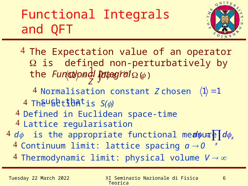
( )1( )Sd e
Z
The Expectation value of an operator is defined non-perturbatively by the Functional Integral
The action is S()
1 1 Normalisation constant Z chosen such that
xx
d d d is the appropriate functional measure Continuum limit: lattice spacing a 0 Thermodynamic limit: physical volume V
Defined in Euclidean space-time Lattice regularisation

Wednesday 19 April 2023 XI Seminario Nazionale di Fisica Teorica 7
Monte Carlo Integration
Monte Carlo integration is based on the identification of probabilities with measures
There are much better methods of carrying out low dimensional quadrature
All other methods become hopelessly expensive for large dimensions
In lattice QFT there is one integration per degree of freedom We are approximating an infinite dimensional functional
integral
Wednesday 19 April 2023 XI Seminario Nazionale di Fisica Teorica 8
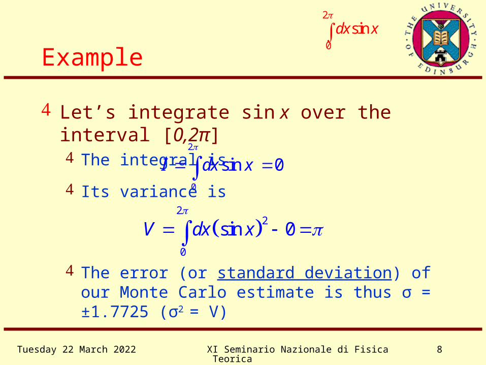
Example
Let’s integrate sin x over the interval [0,2π] The integral is
2
0
sin 0I dx x
Its variance is
2
2
0
sin 0V dx x
The error (or standard deviation) of our Monte
Carlo estimate is thus σ = ±1.7725 (σ2 = V)
2
0
sindx x
Wednesday 19 April 2023 XI Seminario Nazionale di Fisica Teorica 9
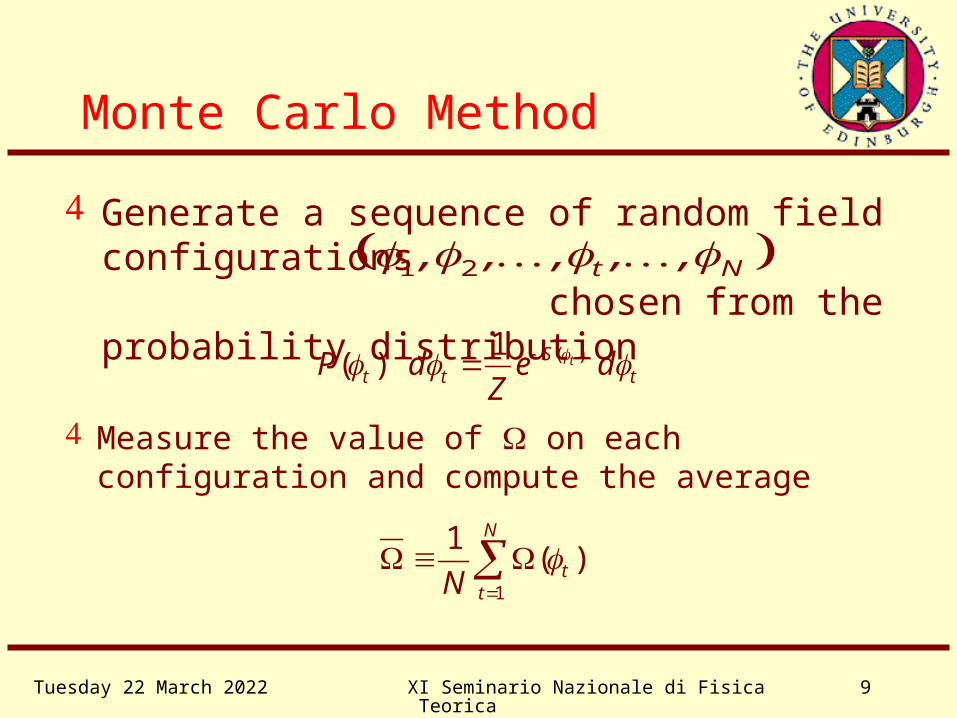
Measure the value of on each configuration and compute the average
1
1( )
N
ttN
Monte Carlo Method
Generate a sequence of random field configurations chosen from the probability distribution
1 2 t N, , , , ,
( )1( ) tS
t t tP d e dZ

Wednesday 19 April 2023 XI Seminario Nazionale di Fisica Teorica 10
Central Limit Theorem
The Laplace–DeMoivre Central Limit theorem is an asymptotic expansion for the probability distribution of Distribution of values for a single sample = ()
( )P d P
Central Limit Theorem
The variance of the distribution of is
2CNO
2
2C
Law of Large Numbers limN

Wednesday 19 April 2023 XI Seminario Nazionale di Fisica Teorica 11
3
0 3
4 21 4 2
2
2
0
3
C C
C C C
C
The first few cumulants are
Cumulant Expansion
Note that this is an
asymptotic expansion
Generating function for connected moments( ) ln ( ) ikW k d P e
ln lnik ikd P e e
0 !
n
nn
ikC
n

Wednesday 19 April 2023 XI Seminario Nazionale di Fisica Teorica 12
Distribution of the Average
lnN
ik Nd P e
1 11
ln expN
N N tt
ikd d P P
N
Connected generating function( ) ln ( ) ikW k d P e
1
1 !
n
nn
n
ik C
n N
ln ik NN e
kNW
N
1 11
1 N
N N tt
P d d P PN
Distribution of the average of N samples
Wednesday 19 April 2023 XI Seminario Nazionale di Fisica Teorica 13
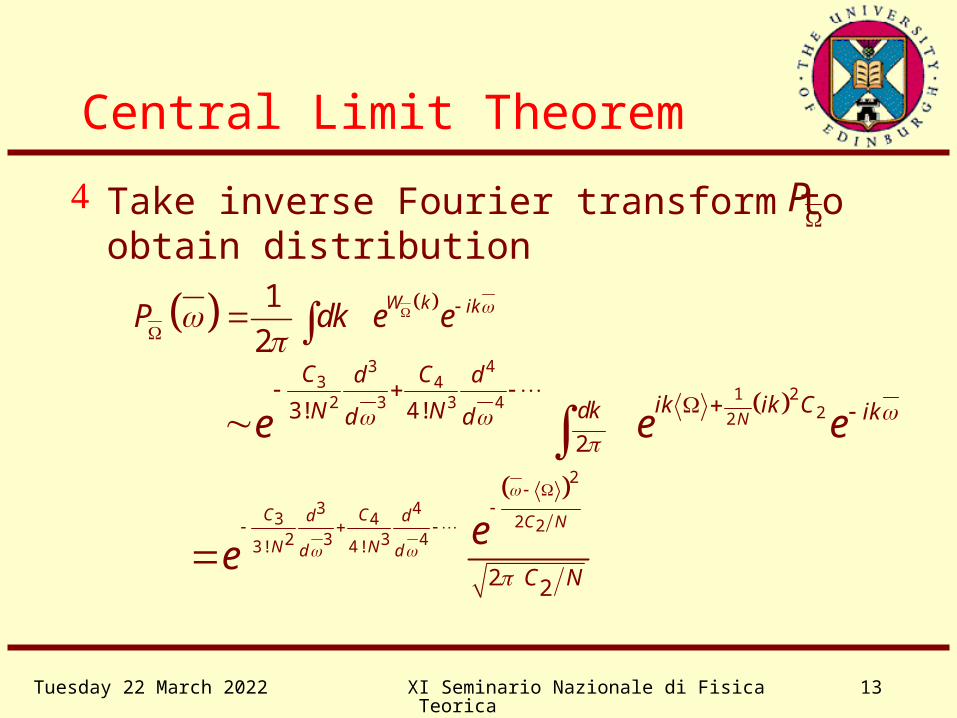
Central Limit Theorem
3 4
3 4212 3 3 4
223! 4!
2N
C Cd dik ik CdkN N ikd de e e
Take inverse Fourier transform to obtain distribution
P
1
2W k ikP dk e e
2
3 43 4 2 2
2 3 3 43! 4 !
2 2
C Cd d C N
N Nd d
C N
ee
Wednesday 19 April 2023 XI Seminario Nazionale di Fisica Teorica 14
Central Limit Theorem

Wednesday 19 April 2023 XI Seminario Nazionale di Fisica Teorica 15
Central Limit Theorem
where and N
2
22 2
3 2
32 2
31
6 2
CC C eF
C N C
dP F
d
Re-scale to show convergence to Gaussian distribution
Wednesday 19 April 2023 XI Seminario Nazionale di Fisica Teorica 16
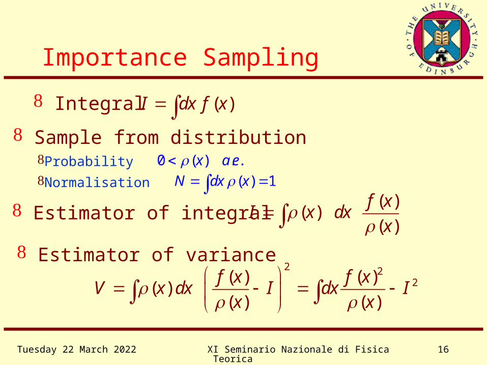
Importance Sampling
Sample from distributionProbability
Normalisation ( ) 1N dx x 0 ( ) . .x a e
( )I dx f x Integral
( )( )
( )
f xI x dx
x
Estimator of integral
2 22( ) ( )
( )( ) ( )
f x f xV x dx I dx I
x x
Estimator of variance

Wednesday 19 April 2023 XI Seminario Nazionale di Fisica Teorica 17
Optimal Importance Sampling
2
2
( ) ( )0
( ) ( )
V N f y
y y
Minimise variance
Constraint N=1Lagrange multiplier
( )( )
( )opt
f xx
dx f x
Optimal measure
Optimal variance
2 2
opt ( ) ( )V dx f x dx f x

Wednesday 19 April 2023 XI Seminario Nazionale di Fisica Teorica 18
( ) sinf x x Example
14( ) sinx x Optimal weight
2 22 2
opt0 0
sin( ) sin( ) 16V dx x dx x
Optimal variance
Example
2
0
sindx x
Wednesday 19 April 2023 XI Seminario Nazionale di Fisica Teorica 19
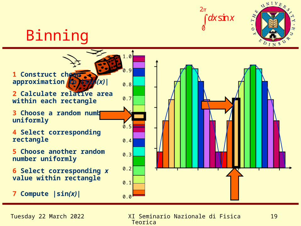
Binning
1 Construct cheap approximation to |sin(x)|
2 Calculate relative area within each rectangle
5 Choose another random number uniformly
4 Select corresponding rectangle
3 Choose a random number uniformly
6 Select corresponding x value within rectangle
7 Compute |sin(x)|
2
0
sindx x
1.0
0.9
0.7
0.5
0.3
0.4
0.6
0.8
0.2
0.1
0.0
Wednesday 19 April 2023 XI Seminario Nazionale di Fisica Teorica 20
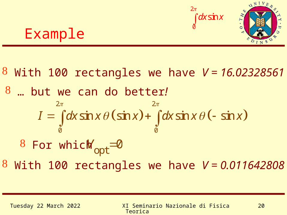
Example
2 2
0 0
sin sin sin sinI dx x x dx x x
… but we can do better!
opt 0V For which
With 100 rectangles we have V = 16.02328561
With 100 rectangles we have V = 0.011642808
2
0
sindx x

Wednesday 19 April 2023 XI Seminario Nazionale di Fisica Teorica 21
Markov chains
State space (Ergodic) stochastic transitions P’:
Distribution converges to unique fixed point Q
Deterministic evolution of probability distribution P: Q Q

Wednesday 19 April 2023 XI Seminario Nazionale di Fisica Teorica 22
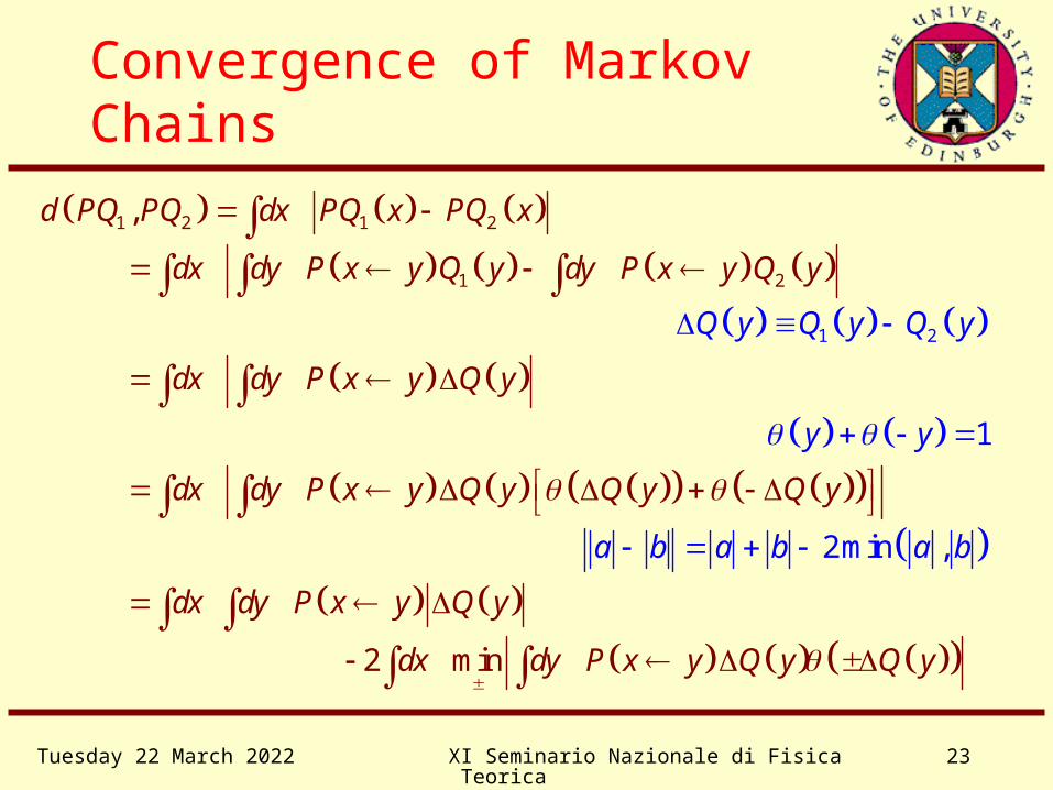
Convergence of Markov Chains
The sequence Q, PQ, P2Q, P3Q,… is Cauchy
Define a metric on the space of (equivalence classes of) probability distributions
1 2 1 2,d Q Q dx Q x Q x
Prove that with > 0, so the Markov process P is a contraction mapping
1 2 1 2, 1 ,d PQ PQ d Q Q
The space of probability distributions is complete, so the sequence converges to a unique fixed point distribution lim n
nQ P Q
Wednesday 19 April 2023 XI Seminario Nazionale di Fisica Teorica 23
Convergence of Markov Chains
1 2 1 2,d PQ PQ dx PQ x PQ x 1 2dx dy P x y Q y dy P x y Q y
dx dy P x y Q y Q y Q y
dx dy P x y Q y
2 mindx dy P x y Q y Q y
dx dy P x y Q y
2min ,a b a b a b
1 2Q y Q y Q y
1y y

Wednesday 19 April 2023 XI Seminario Nazionale di Fisica Teorica 24
Convergence of Markov Chains
2 mindy Q y dx dy P x y Q y Q y
2 inf min
ydy Q y dx P x y dy Q y Q y
infy
dy Q y dx P x y dy Q y 1 2,d Q Q
1 2 1 1 0dy Q y dy Q y dy Q y dy Q y Q y dy Q y Q y
1dx P x y
12dy Q y Q y dy Q y
0 1 inf 1y
dx P x y
1 2,d PQ PQ

Wednesday 19 April 2023 XI Seminario Nazionale di Fisica Teorica 25
Use of Markov Chains
Use Markov chains to sample from Q Suppose we can construct an ergodic Markov process P
which has distribution Q as its fixed point Start with an arbitrary state (“field configuration”) Iterate the Markov process until it has converged
(“thermalized”) Thereafter, successive configurations will be distributed
according to Q But in general they will be correlated
To construct P we only need relative probabilities of states Don’t know the normalisation of Q Cannot use Markov chains to compute integrals directly We can compute ratios of integrals

Wednesday 19 April 2023 XI Seminario Nazionale di Fisica Teorica 26
Metropolis Algorithm
How do we construct a Markov process with a specified fixed point? Q x dy P x y Q y
integrate w.r.t. y to obtain fixed point condition sufficient but not necessary for fixed point
P y x Q x P x y Q y Detailed balance
consider cases Q(x)>Q(y) and Q(x)<Q(y) separately to obtain detailed balance condition
sufficient but not necessary for detailed balance
Metropolis algorithm min 1,P x y Q x Q y
Q xP x y
Q x Q y
other choices are possible, e.g.,

Wednesday 19 April 2023 XI Seminario Nazionale di Fisica Teorica 27
Composite Markov Steps
Composition of Markov steps Let P1 and P2 be two Markov steps which have the desired
fixed point distribution... … they need not be ergodic Then the composition of the two steps P1P2 will also have the
desired fixed point... … and it may be ergodic
This trivially generalises to any (fixed) number of steps For the case where P is not ergodic but Pn is the terminology
“weakly” and “strongly” ergodic are sometimes used

Wednesday 19 April 2023 XI Seminario Nazionale di Fisica Teorica 28
Site-by-Site Updates
This result justifies “sweeping” through a lattice performing single site updates Each individual single site update has the desired fixed point
because it satisfies detailed balance The entire sweep therefore has the desired fixed point, and
is ergodic... … but the entire sweep does not satisfy detailed balance Of course it would satisfy detailed balance if the sites were
updated in a random order… … but this is not necessary … and it is undesirable because it puts too much
randomness into the system

Wednesday 19 April 2023 XI Seminario Nazionale di Fisica Teorica 29
Exponential Autocorrelations
This corresponds to the exponential autocorrelation time exp
max
10
lnN
The unique fixed point of an ergodic Markov process corresponds to the unique eigenvector with eigenvalue 1
All its other eigenvalues must lie within the unit circle
In particular, the largest subleading eigenvalue is |λmax|<1

Wednesday 19 April 2023 XI Seminario Nazionale di Fisica Teorica 30
Integrated Autocorrelations
2
21 1
1 N N
t tt tN
1
2
21 1 1
12
N N N
t t tt t t tN
Consider autocorrelation of some operator Ω
0 Without loss of generality we may assume
12 2 2
1
1 2 N
N CN N
2
t tC
Define the autocorrelation function
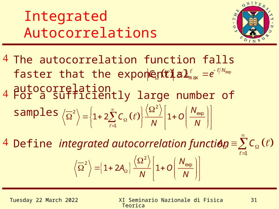
Wednesday 19 April 2023 XI Seminario Nazionale di Fisica Teorica 31
Integrated Autocorrelations
The autocorrelation function falls faster that the exponential autocorrelation exp
maxNC e
2
2 exp
1
1 2 1N
C ON N
2
2 exp1 2 1N
A ON N
For a sufficiently large number of samples
1
A C
Define integrated autocorrelation function
Wednesday 19 April 2023 XI Seminario Nazionale di Fisica Teorica 32
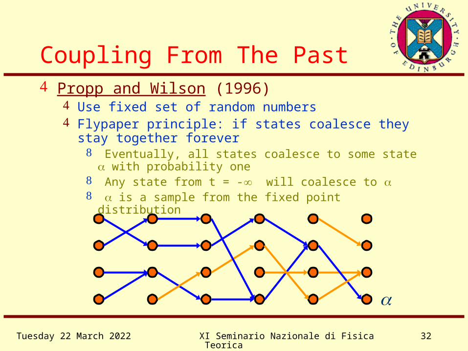
Coupling From The Past Propp and Wilson (1996)
Use fixed set of random numbers Flypaper principle: if states coalesce they stay together
forever Eventually, all states coalesce to some state with probability
one Any state from t = - will coalesce to is a sample from the fixed point distribution
Wednesday 19 April 2023 XI Seminario Nazionale di Fisica Teorica 33
Continuum Limits
We are not interested in lattice QFTs per se, but in their continuum limit as a 0 This corresponds to a continuous phase transition of the
discrete lattice model For the continuum theory to have a finite correlation length a
(inverse mass gap) in physical units this correlation length must diverge in lattice units
We expect such systems to exhibit universal behaviour as they approach a continuous phase transition
The nature of the continuum theory is characterised by its symmetries
The details of the microscopic interactions are unimportant at macroscopic length scales
Universality is a consequence of the way that the the theory scales as a 0 while a is kept fixed

Wednesday 19 April 2023 XI Seminario Nazionale di Fisica Teorica 34
Continuum Limits
The nature of the continuum field theory depends on the way that physical quantities behave as the system approaches the continuum limit
The scaling of the parameters in the action required is described by the renormalisation group equation (RGE)
The RGE states the “reparameterisation invariance” of the theory as the choice of scale at which we choose to fix the renormalisation conditions
As a 0 we expect the details of the regularisation scheme (cut off effects, lattice artefacts) to vanish, so the effect of changing a is just an RGE transformation
On the lattice the a renormalisation group transformation may be implemented as a “block spin” transformation of the fields
Strictly speaking, the renormalisation “group” is a semigroup on the lattice, as blockings are not invertible

Wednesday 19 April 2023 XI Seminario Nazionale di Fisica Teorica 35
Continuum Limits
The continuum limit of a lattice QFT corresponds to a fixed point of the renormalisation group
At such a fixed point the form of the action does not change under an RG transformation
The parameters in the action scale according to a set of critical exponents
All known four dimensional QFTs correspond to trivial (Gaussian) fixed points
For such a fixed point the UV nature of the theory may by analysed using perturbation theory
Monomials in the action may be classified according to their power counting dimension
d < 4 relevant (superrenormalisable) d = 4 marginal (renormalisable) d > 4 irrelevant (nonrenormalisable)
Wednesday 19 April 2023 XI Seminario Nazionale di Fisica Teorica 36
The behaviour of our Markov chains as the system approaches a continuous phase transition is described by its dynamical critical exponents these describe how badly the system (model + algorithm)
undergo critical slowing down
Continuum Limits
the dynamical critical exponent z tells us how the cost of generating an independent configuration grows as the correlation length of the system is taken to , cost z
this is closely related (but not always identical) to the dynamical critical exponent for the exponential or integrated autocorrelations

Wednesday 19 April 2023 XI Seminario Nazionale di Fisica Teorica 37
Global Heatbath
The ideal generator selects field configurations randomly and independently from the desired distribution It is hard to construct such global heatbath generators for
any but the simplest systems They can be built by selecting sufficiently independent
configurations from a Markov process… … or better yet using CFTP which guarantees that the
samples are truly uncorrelated But this such generators are expensive!

Wednesday 19 April 2023 XI Seminario Nazionale di Fisica Teorica 38
Global Heatbath
For the purposes of Monte Carlo integration these is no need for the configurations to be completely uncorrelated We just need to take the autocorrelations into account in our
estimate of the variance of the resulting integral Using all (or most) of the configurations generated by a
Markov process is more cost-effective than just using independent ones
The optimal choice balances the cost of applying each Markov step with the cost of making measurements

Wednesday 19 April 2023 XI Seminario Nazionale di Fisica Teorica 39
Local Heatbath
For systems with a local bosonic action we can build a Markov process with the fixed point distribution exp(-S) out of steps which update a single site with this fixed point
If this update generates a new site variable value which is completely independent of its old value then it is called a local heatbath
For free field theory we just need to generate a Gaussian-distributed random variable

Wednesday 19 April 2023 XI Seminario Nazionale di Fisica Teorica 40
Gaussian Generators
If are uniformly distributed
random numbers then is approximately
Gaussian by the Central Limit theorem
1 2, , , nx x x1
1
n
jnj
x
This is neither cheap nor accurate

Wednesday 19 April 2023 XI Seminario Nazionale di Fisica Teorica 41
Gaussian Generators
1 1
1dP y dx y f x y
f f f f y
If x is uniformly distributed and f is a monotonically increasing function then f(x) is distributed as
Choosing we obtain 2lnf x x 21
2y
P y y e
Therefore generate two uniform random numbers x1
and x2, set ,
then are two independent
Gaussian distributed random numbers
1 22ln , 2r x x
1 2cos , siny r y r
Wednesday 19 April 2023 XI Seminario Nazionale di Fisica Teorica 42
Gaussian Generators
Even better methods exist The Rectangle-Wedge-Tail (RWT) method The Ziggurat method These do not require special function evaluations They can be more interesting to implement for
parallel computers
Wednesday 19 April 2023 XI Seminario Nazionale di Fisica Teorica 43
Local Heatbath
For pure gauge theories the field variables live on the links of the lattice and take their values in a representation of the gauge group For SU(2) Creutz gave an exact local heatbath algorithm
It requires a rejection test: this is different from the Metropolis accept/reject step in that one must continue generating candidate group elements until one is accepted
For SU(3) the “quasi-heatbath” method of Cabibbo and Marinari is widely used
Update a sequence of SU(2) subgroups This is not quite an SU(3) heatbath method… … but sweeping through the lattice updating SU(2) subgroups is also a
valid algorithm, as long as the entire sweep is ergodic For a higher acceptance rate there is an alternative SU(2) subgroup
heatbath algorithm

Wednesday 19 April 2023 XI Seminario Nazionale di Fisica Teorica 44
Hybrid Monte Carlo
In order to carry out Monte Carlo computations including the effects of dynamical fermions we would like to find an algorithm which Updates the fields globally
Because single link updates are not cheap if the action is not local
Takes large steps through configuration space Because small-step methods carry out a random walk which
leads to critical slowing down with a dynamical critical exponent z=2
Does not introduce any systematic errors
Wednesday 19 April 2023 XI Seminario Nazionale di Fisica Teorica 45
Hybrid Monte Carlo
A useful class of algorithms with these properties is the (Generalised) Hybrid Monte Carlo (HMC) method Introduce a “fictitious momentum” p corresponding to each
dynamical degree of freedom q Find a Markov chain with fixed point exp[-H(q,p)] where H
is the “fictitious Hamiltonian” ½ p2 + S(q) The action S of the underlying QFT plays the rôle of the
potential in the “fictitious” classical mechanical system This gives the evolution of the system in a fifth dimension,
“fictitious” or computer time
This generates the desired distribution exp[-S(q)] if we ignore the momenta q (i.e., the marginal distribution)

Wednesday 19 April 2023 XI Seminario Nazionale di Fisica Teorica 46
Hybrid Monte Carlo
The GHMC Markov chain alternates two Markov steps Molecular Dynamics Monte Carlo (MDMC) Partial Momentum Refreshment
Both have the desired fixed point Together they are ergodic

Wednesday 19 April 2023 XI Seminario Nazionale di Fisica Teorica 47
Molecular Dynamics
If we could integrate Hamilton’s equations exactly we could follow a trajectory of constant fictitious energy This corresponds to a set of equiprobable fictitious phase
space configurations Liouville’s theorem tells us that this also preserves the
functional integral measure dp dq as required
Any approximate integration scheme which is reversible and area preserving may be used to suggest configurations to a Metropolis accept/reject test With acceptance probability min[1,exp(-H)]
Wednesday 19 April 2023 XI Seminario Nazionale di Fisica Teorica 48
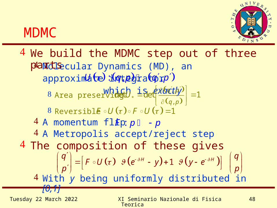
MDMC
Molecular Dynamics (MD), an approximate integrator which is exactly : , ,U q p q p
We build the MDMC step out of three parts
A Metropolis accept/reject step
Area preserving *
,
,det det 1
q p
q pU
Reversible 1F U F U
A momentum flip :F p p
1H Hq qF U e y y e
p p
The composition of these gives
With y being uniformly distributed in [0,1]

Wednesday 19 April 2023 XI Seminario Nazionale di Fisica Teorica 49
Momentum Refreshment
The Gaussian distribution of p is invariant under F the extra momentum flip F ensures that for small
the momenta are reversed after a rejection rather than after an acceptance
for =/2 all momentum flips are irrelevant
This mixes the Gaussian distributed momenta p with Gaussian noise
cos sin
sin cos
p pF
Wednesday 19 April 2023 XI Seminario Nazionale di Fisica Teorica 50
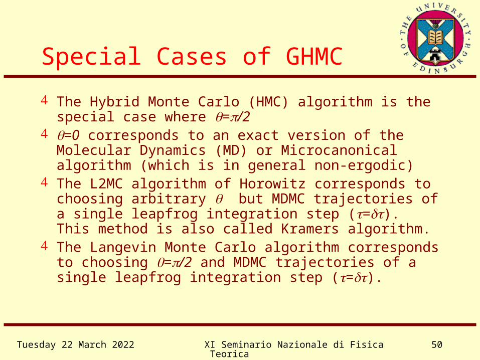
Special Cases of GHMC
The Hybrid Monte Carlo (HMC) algorithm is the special case where =/2
=0 corresponds to an exact version of the Molecular Dynamics (MD) or Microcanonical algorithm (which is in general non-ergodic)
The L2MC algorithm of Horowitz corresponds to choosing arbitrary but MDMC trajectories of a single leapfrog integration step (=). This method is also called Kramers algorithm.
The Langevin Monte Carlo algorithm corresponds to choosing =/2 and MDMC trajectories of a single leapfrog integration step (=).
Wednesday 19 April 2023 XI Seminario Nazionale di Fisica Teorica 51
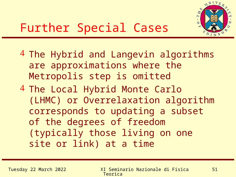
Further Special Cases
The Hybrid and Langevin algorithms are approximations where the Metropolis step is omitted
The Local Hybrid Monte Carlo (LHMC) or Overrelaxation algorithm corresponds to updating a subset of the degrees of freedom (typically those living on one site or link) at a time
Wednesday 19 April 2023 XI Seminario Nazionale di Fisica Teorica 52
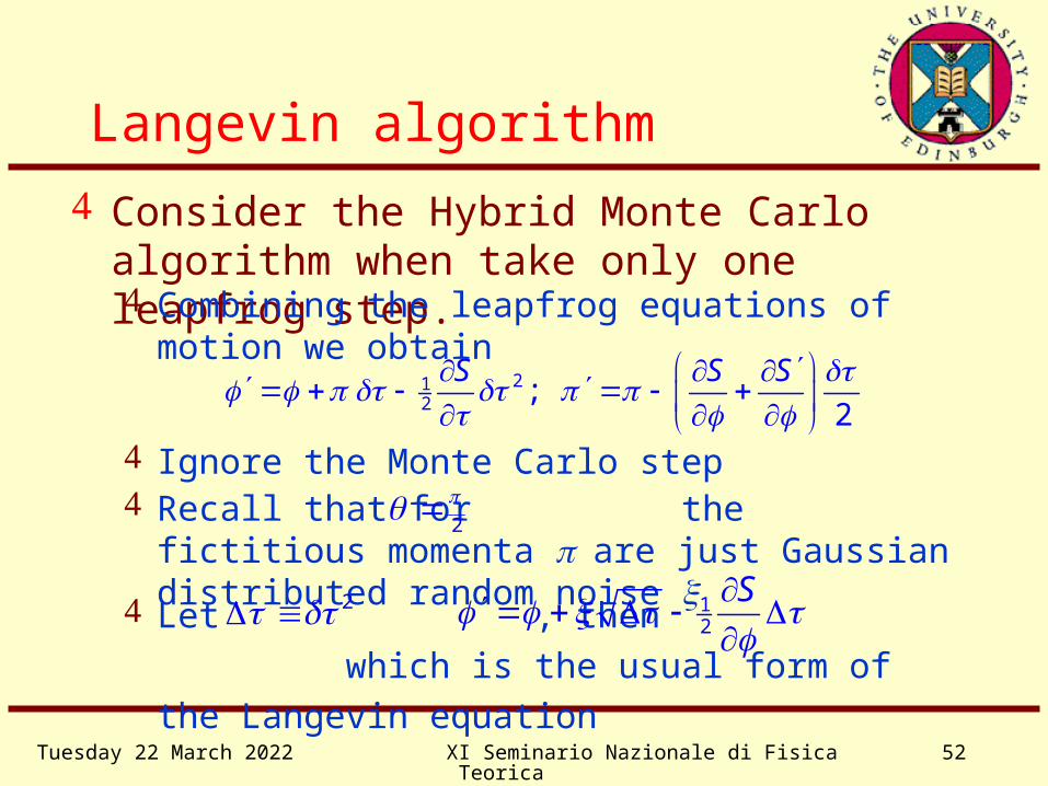
Consider the Hybrid Monte Carlo algorithm when take only one leapfrog step.
Langevin algorithm
212 ;
2
S S S
Combining the leapfrog equations of motion we obtain
Ignore the Monte Carlo step Recall that for the fictitious momenta are
just Gaussian distributed random noise 2
Let , then which is
the usual form of the Langevin equation
2 12
S

Wednesday 19 April 2023 XI Seminario Nazionale di Fisica Teorica 53
What happens if we omit the Metropolis test?
Inexact algorithms
We still have an ergodic algorithm, so there is
some unique fixed point distribution
which will be generated by the algorithm
S Se
The condition for this to be a fixed point is
212
S S S Se d e d e U
Wednesday 19 April 2023 XI Seminario Nazionale di Fisica Teorica 54
Langevin Algorithm
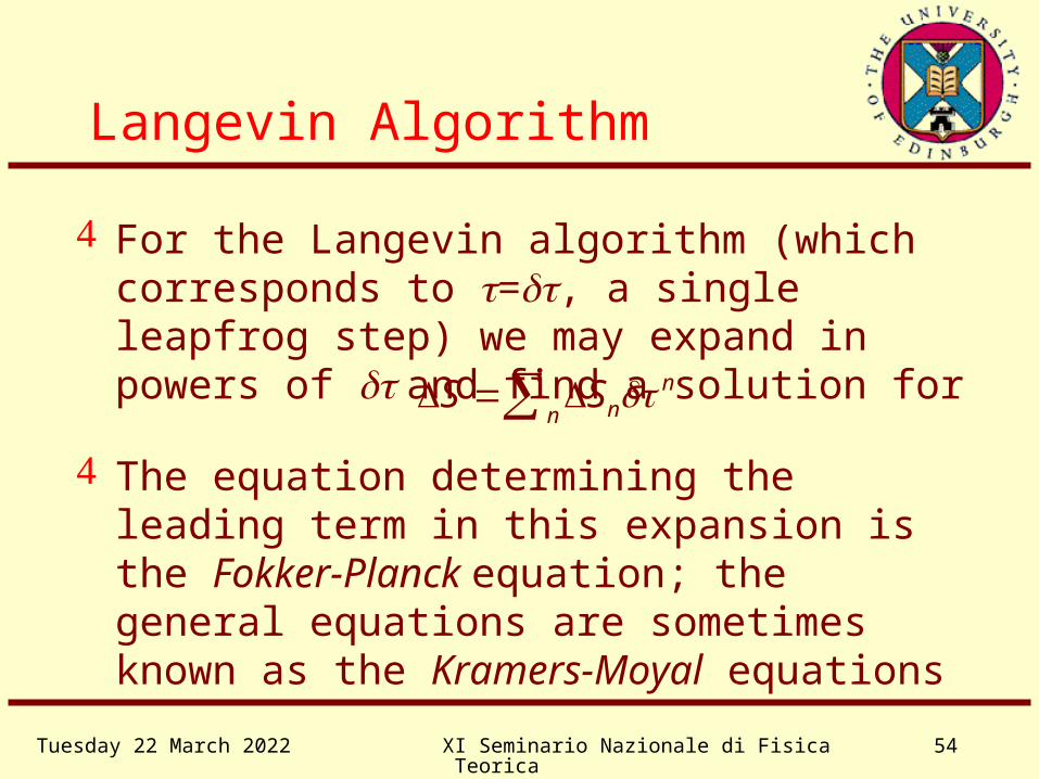
For the Langevin algorithm (which corresponds to =, a single leapfrog step) we may expand in powers of and find a solution for
nnn
S S The equation determining the leading term in
this expansion is the Fokker-Planck equation; the general equations are sometimes known as the Kramers-Moyal equations
Wednesday 19 April 2023 XI Seminario Nazionale di Fisica Teorica 55
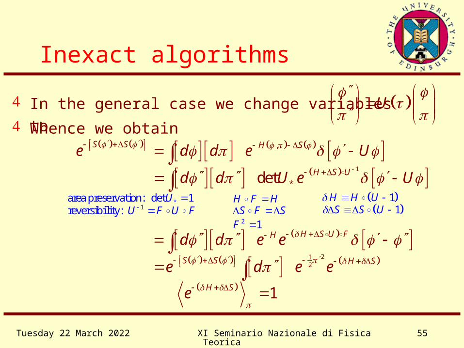
Inexact algorithms
In the general case we change variables to U
Whence we obtain
,S S H Se d d e U
1
*det H S Ud d U e U
H S U FHd d e e
212
S S H Se d e e
1H Se
2 1F
1reversibility: U F U F *area preservation: det 1U H F H
S F S 1H H U 1S S U

Wednesday 19 April 2023 XI Seminario Nazionale di Fisica Teorica 56
Inexact algorithms
Since H is extensive so is H, and thus so is
the connected generating function (cumulants) ,F He e
We can thus show order by order in that S
is extensive too

Wednesday 19 April 2023 XI Seminario Nazionale di Fisica Teorica 57
Langevin Algorithm For the Langevin algorithm we have
and , so we immediately find that
4H O
2nS O
2S O 22
21 12 8 82
2 2 j j jj jj
S SS S S
14 48 2 2ijjkk ijjk k ijk j k ijk ijki
S S S S S S S S S If S is local then so are all the Sn
We only have an asymptotic expansion for S, and in general the subleading terms are neither local nor extensive
Therefore, taking the continuum limit a 0 limit for fixed will probably not give exact results for renormalised quantities

Wednesday 19 April 2023 XI Seminario Nazionale di Fisica Teorica 58
Hybrid Algorithm
0nS O
For the Hybrid algorithm and
so again we find
2H O
2S O
We have made use of the fact that H’ is conserved
and differs from H by O(δτ2)

Wednesday 19 April 2023 XI Seminario Nazionale di Fisica Teorica 59
Inexact algorithms
What effect do such systematic errors in the
distribution have on measurements?
If we want to improve the action so as to reduce lattice
discretisation effects and get a better approximation to the
underlying continuum theory, then we have to ensure that
for the appropriate n2 n«a
Large errors will occur where observables are discontinuous
functions of the parameters in the action, e.g., near phase
transitions
Step size errors need not be irrelevant
Wednesday 19 April 2023 XI Seminario Nazionale di Fisica Teorica 60
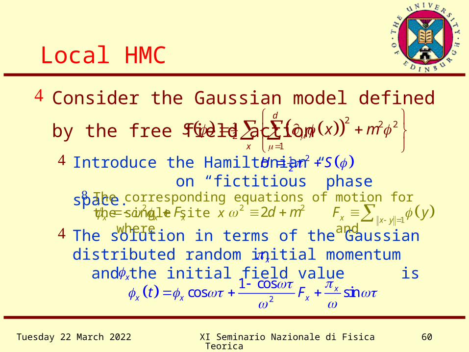
Local HMC
Consider the Gaussian model defined by the
free field action 2 2 212
1
d
x
S x m
2
1 coscos sinx
x x xt F
The solution in terms of the Gaussian distributed random initial momentum and the initial field value is
xx
Introduce the Hamiltonian on “fictitious” phase space.
212H S
The corresponding equations of motion for the single site x where and2
x x xF 1x x y
F y
2 22d m

Wednesday 19 April 2023 XI Seminario Nazionale di Fisica Teorica 61
Local HMC Identify and to get the usual Adler
overrelaxation update1 cos x
2
21
Fx x
For gauge theories various overrelaxation methods have been suggested Hybrid Overrelaxation: this alternates a heatbath step with
many overrelaxation steps with =2
LHMC: this uses an analytic solution for the equations of motion for the update of a single U(1) or SO(2) subgroup at a time. In this case the equations of motion may be solved in terms of elliptic functions

Wednesday 19 April 2023 XI Seminario Nazionale di Fisica Teorica 62
Classical Mechanics onGroup Manifolds Gauge fields take their values in some Lie group, so
we need to define classical mechanics on a group manifold which preserves the group-invariant Haar measure A Lie group G is a smooth manifold on which there is a natural
mapping L: G G G defined by the group action This induces a map called the pull-back of L on the cotangent
bundle defined by
* *
** *
* * * **
:
:
:
g g
g g
g g
L G F F L f f L
L G TG TG L v f v L f
L G T G T G L v L v
F is the space of 0 forms, which are smooth mappings from G to the real numbers :F G

Wednesday 19 April 2023 XI Seminario Nazionale di Fisica Teorica 63
*L A form is left invariant if The tangent space to a Lie group at the origin is called the Lie
algebra, and we may choose a set of basis vectors which satisfy the commutation relations where are the structure constants of the algebra
0ie, k
i j ij kk
e e c e kijc
We may define a set of left invariant vector fields on TG by * 0i g ie g L e
The corresponding left invariant dual forms satisfy the Maurer-Cartan equations 1
2i i j k
jkjk
d c i
We may therefore define a closed symplectic 2 form which globally defines an invariant Poisson bracket by
12
i i i i i i i i i i j kjk
i i i
d p dp p d dp p c
Classical Mechanics onGroup Manifolds

Wednesday 19 April 2023 XI Seminario Nazionale di Fisica Teorica 64
We may now follow the usual procedure to find the equations of motion Introduce a Hamiltonian function (0 form) H on the cotangent
bundle (phase space) over the group manifold ,dH y h y y TG Define a vector field h such that
iii i
i
y y e yp
iii i
i
h h e hp
,i i ii i i i i j k
i jkii i jk
HdH y e H y y h y h y y h p c h y
p
In the natural basis we have
The classical trajectories are then the integral curves of h:
,t t tQ P t th s
Classical Mechanics onGroup Manifolds

Wednesday 19 April 2023 XI Seminario Nazionale di Fisica Teorica 65
k ki ji ii j i
i jk
H Hh e c p e H
p p p
Equating coefficients of the components of y we find
,j j j i i kt i t kj t ji k k
i k i
H H HQ e P c P e
p p q
The equations of motion in the local coordinate
basis are thereforeijj j
j
e eq
,j j j kt i t ji k
i k
H HQ e P e
p q
Which for a Hamiltonian of the form reduce to
2H f p S q
Classical Mechanics onGroup Manifolds

Wednesday 19 April 2023 XI Seminario Nazionale di Fisica Teorica 66
In terms of constrained variables
i
ii
q T
U q e
00
i ii gg
U gT e g U g
g
The representation of the generators is
i ie U UT From which it follows that
††i i iab ab
iab ab ab
U PU
S SP T UT TU T S U U
U U
And for the Hamiltonian leads to the equations of motion
212
i
i
H p S U
For the case G = SU(n) the operator T is the projection onto traceless antihermitian matrices
Classical Mechanics onGroup Manifolds
Wednesday 19 April 2023 XI Seminario Nazionale di Fisica Teorica 67
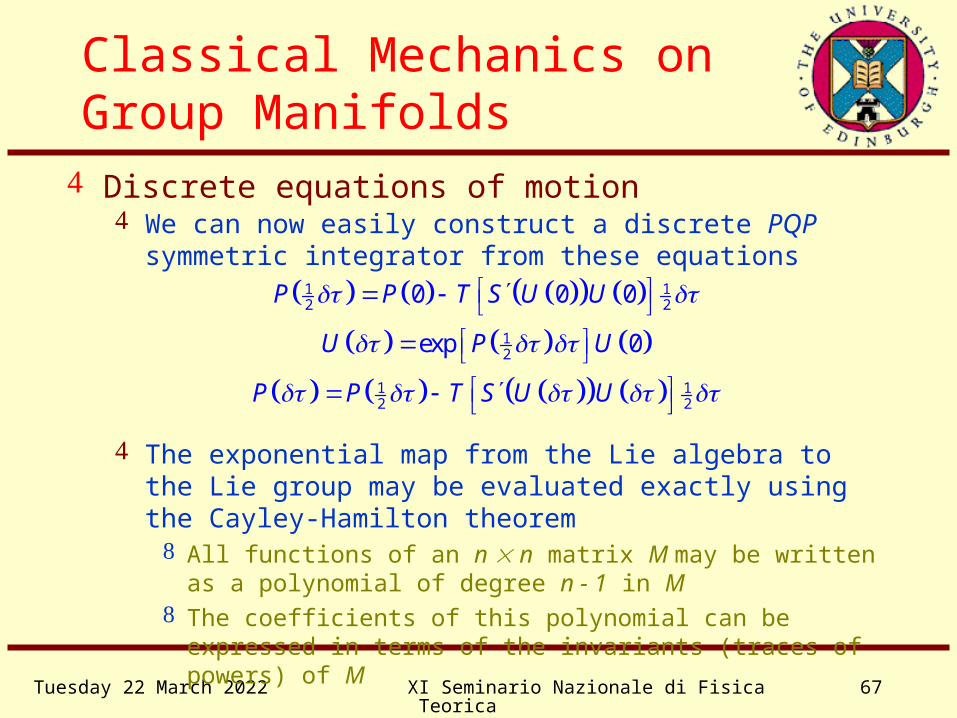
Discrete equations of motion
1 12 2
12
1 12 2
0 0 0
exp 0
P P T S U U
U P U
P P T S U U
We can now easily construct a discrete PQP symmetric integrator from these equations
The exponential map from the Lie algebra to the Lie group may be evaluated exactly using the Cayley-Hamilton theorem
All functions of an n n matrix M may be written as a polynomial of degree n - 1 in M
The coefficients of this polynomial can be expressed in terms of the invariants (traces of powers) of M
Classical Mechanics onGroup Manifolds
Wednesday 19 April 2023 XI Seminario Nazionale di Fisica Teorica 68
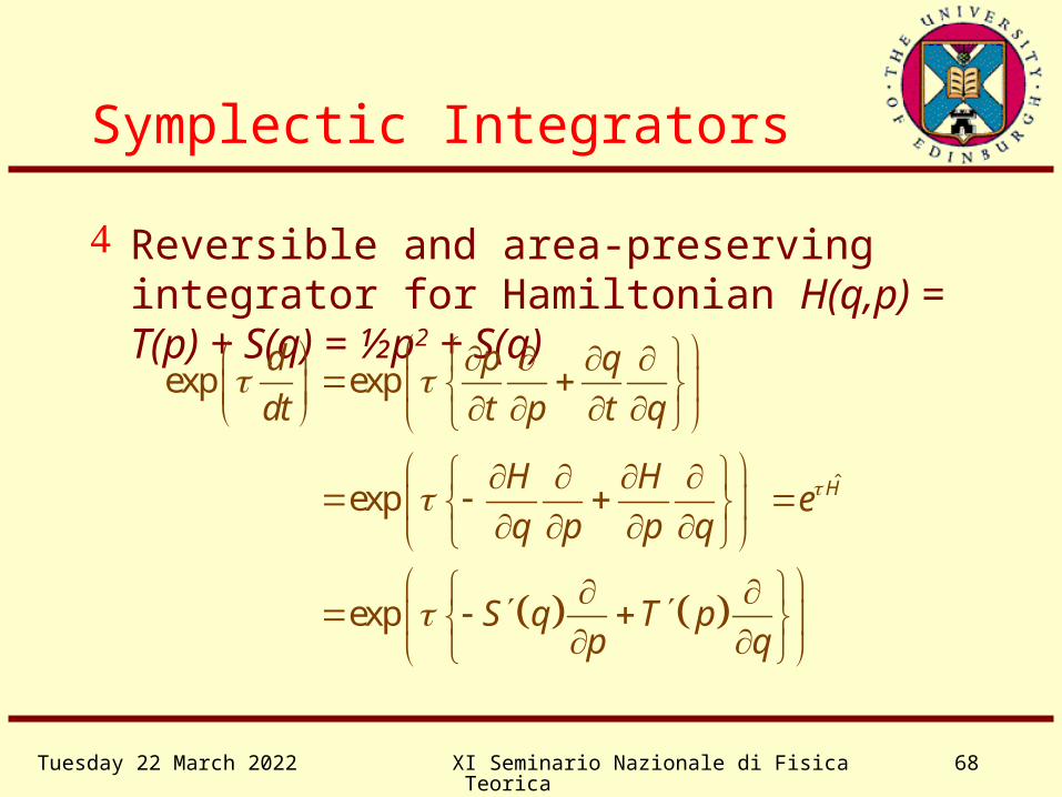
Symplectic Integrators
Reversible and area-preserving integrator for Hamiltonian H(q,p) = T(p) + S(q) = ½p2 + S(q)
exp expd p q
dt t p t q
expH H
q p p q
He
exp S q T pp q
Wednesday 19 April 2023 XI Seminario Nazionale di Fisica Teorica 69
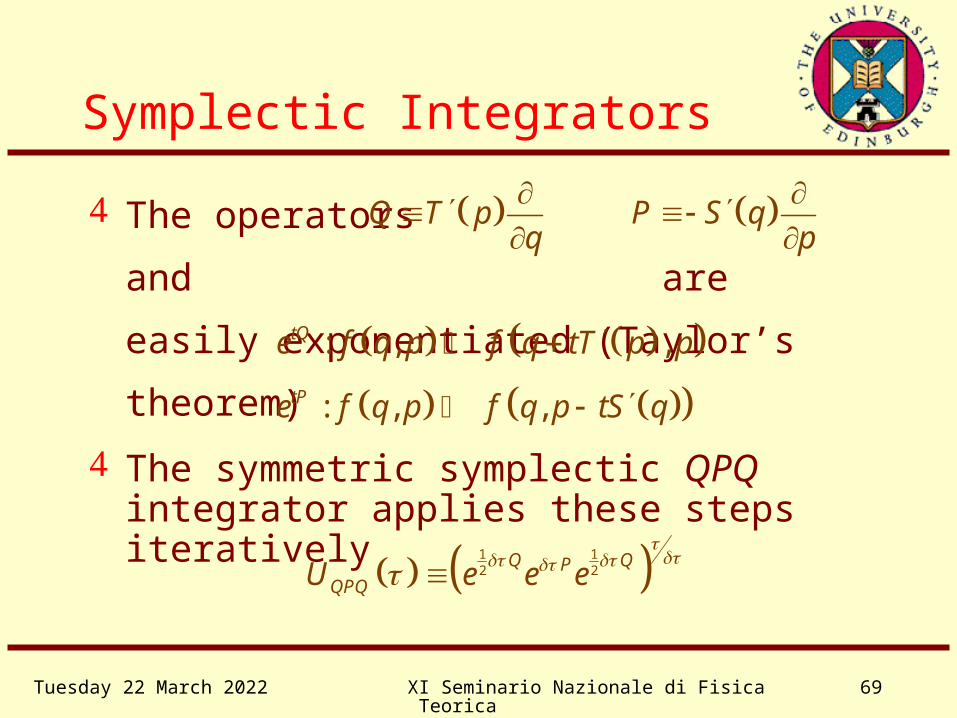
Symplectic Integrators
1 12 2
Q QPQPQU e e e
The operators and
are easily exponentiated (Taylor’s theorem)
Q T pq
P S qp
: , ,tQe f q p f q tT p p
: , ,tPe f q p f q p tS q
The symmetric symplectic QPQ integrator applies these steps iteratively

Wednesday 19 April 2023 XI Seminario Nazionale di Fisica Teorica 70
BCH Formula
It is in the Free Lie Algebra generated by {A,B}
A B A Be e e
If A and B belong to any (non-commutative)
algebra then , where is
constructed from commutators of A and B
More precisely, where c1=A+B and
1
ln A Bn
n
e e c
1 2
2
1
/ 21
1 21,..., 10
1[ , ] [ ,[...,[ ]...]]
1 2 !{ }
m
m
m
nm
n n k kk km
k k n
Bc c A B c c A B
n m
The Bm are Bernouilli numbers

Wednesday 19 April 2023 XI Seminario Nazionale di Fisica Teorica 71
BCH Formula
Explicitly, the first few terms are
1 1 12 12 24
1720
ln , , , , , , , ,
, , , , 4 , , , ,
6 , , , , 4 , , , ,
2 , , , , , , , ,
A Be e A B A B A A B B A B B A A B
A A A A B B A A A B
A B A A B B B A A B
A B B A B B B B A B
Wednesday 19 April 2023 XI Seminario Nazionale di Fisica Teorica 72
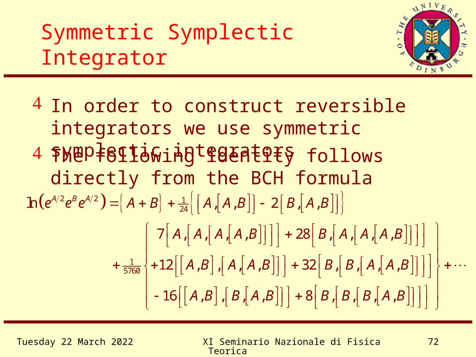
Symmetric Symplectic Integrator
In order to construct reversible integrators we use symmetric symplectic integrators
2 2 124
15760
ln , , 2 , ,
7 , , , , 28 , , , ,
12 , , , , 32 , , , ,
16 , , , , 8 , , , ,
A B Ae e e A B A A B B A B
A A A A B B A A A B
A B A A B B B A A B
A B B A B B B B A B
The following identity follows directly from the BCH formula

Wednesday 19 April 2023 XI Seminario Nazionale di Fisica Teorica 73
Symmetric Symplectic Integrator
1 12 2
Q QPQPQU e e e
3 5124exp , , 2 , ,Q P Q Q P P Q P O
3 4124exp , , 2 , ,Q P Q Q P P Q P O
ˆQPQHe
The BCH formula tells us that the QPQ integrator has evolution

Wednesday 19 April 2023 XI Seminario Nazionale di Fisica Teorica 74
QPQ Integrator
ˆ QPQ QPQQPQ
H HH
p q q p
44 2 2 2 4 615760 7 24 3 96p S p S S S S S O
The QPQ integrator therefore exactly conserves the Hamiltonian , whereQPQH
2 2 2124 2QPQH H p S S So
Note that cannot be written as the sum of a p-dependent kinetic term and a q-dependent potential term
QPQH
Wednesday 19 April 2023 XI Seminario Nazionale di Fisica Teorica 75
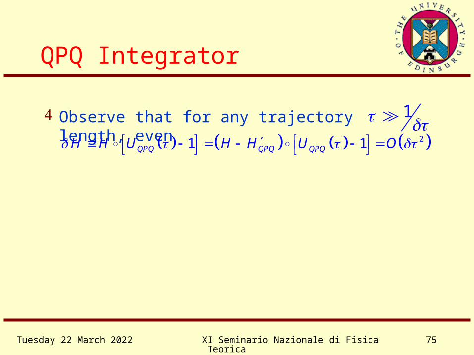
QPQ Integrator
Observe that for any trajectory length, even
21 1QPQ QPQ QPQH H U H H U O
1

Wednesday 19 April 2023 XI Seminario Nazionale di Fisica Teorica 76
Campostrini Wiggles
From the form of the evolution operator Campostrini noted that we can easily write a higher-order integrator
ˆ 3 50 0
HU e R O
ˆ2 3 3 50 0 0 0 2HU U U e R O
3 2 The leading error vanishes if we choose
2
The total step size is unchanged if
This trick may be applied to recursively to obtain arbitrarily high-order symplectic integrators
Wednesday 19 April 2023 XI Seminario Nazionale di Fisica Teorica 77
Instabilities
Consider the simplest leapfrog scheme for a single simple harmonic oscillator with frequency
212
3 21 14 2
1
1
q t q t
p t p t
For a single step we have
The eigenvalues of this matrix are
21 12
cos 12 21 12 41 1
ii e
For > 2 the integrator becomes unstable

Wednesday 19 April 2023 XI Seminario Nazionale di Fisica Teorica 78
Instabilities
The orbits change from ellipses to hyperbolae The energy diverges exponentially in instead of
oscillating For bosonic systems H»1 for such a large
integration step size For light dynamical fermions there seem to be a few
“modes” which have a large force due to the small eigenvalues of the Dirac operator, and this force plays the rôle of the frequency
For these systems is limited by stability rather than by the Metropolis acceptance rate
Wednesday 19 April 2023 XI Seminario Nazionale di Fisica Teorica 79
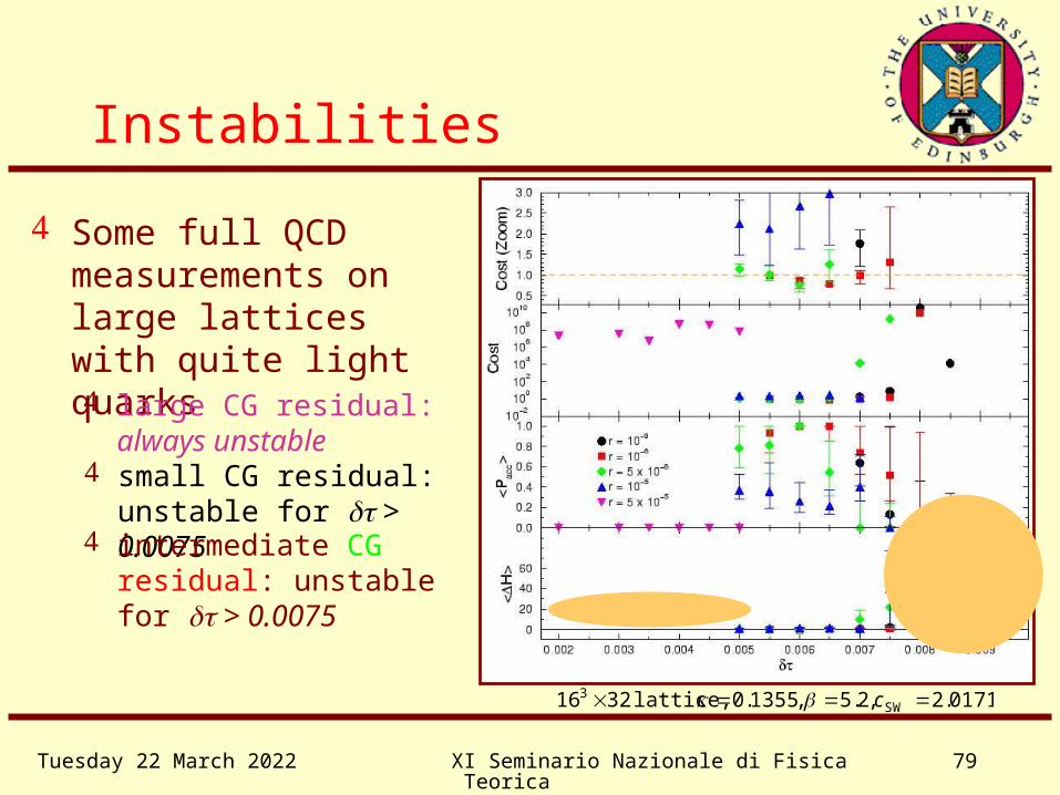
0171.2,2.5,1355.0 lattice, 3216 SW3 c
Instabilities
Some full QCD measurements on large lattices with quite light quarks large CG residual: always
unstable small CG residual:
unstable for > 0.0075 intermediate CG residual:
unstable for > 0.0075
Wednesday 19 April 2023 XI Seminario Nazionale di Fisica Teorica 80
Dynamical Fermions
Fermion fields are Grassmann valued Required to satisfy the spin-statistics theorem Even “classical” Fermion fields obey
anticommutation relations Grassmann algebras behave like negative
dimensional manifolds
Wednesday 19 April 2023 XI Seminario Nazionale di Fisica Teorica 81
Grassmann Algebras
Linear space spanned by generators {1,2,3,…} with coefficients a, b,… in some field (usually the real or complex numbers)
Algebra structure defined by nilpotency condition for elements of the linear space 2 = 0 There are many elements of the algebra which are not in the
linear space (e.g., 12)
Nilpotency implies anticommutativity + = 0 0 = 2 = 2 = ( + )2 = 2 + + + 2 = + = 0
Anticommutativity implies nilpotency 2² = 0 (unless the coefficient field has characteristic 2, i.e., 2 = 0)
Wednesday 19 April 2023 XI Seminario Nazionale di Fisica Teorica 82
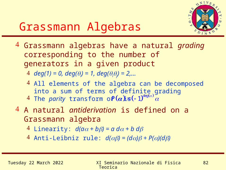
Grassmann algebras have a natural grading corresponding to the number of generators in a given product deg(1) = 0, deg(i) = 1, deg(ij) = 2,...
All elements of the algebra can be decomposed into a sum of terms of definite grading
Grassmann Algebras
The parity transform of is deg1P
A natural antiderivation is defined on a Grassmann algebra Linearity: d(a + b) = a d + b d Anti-Leibniz rule: d() = (d) + P()(d)

Wednesday 19 April 2023 XI Seminario Nazionale di Fisica Teorica 83
Grassmann Integration
Gaussians over Grassmann manifolds Like all functions, Gaussians are polynomials over
Grassmann algebras 1i ij j
ij i ij j
aa
i ij jij ij
e e a
There is no reason for this function to be positive
even for real coefficients
Hence change of variables leads to the inverse
Jacobian 1 1 det in n
j
d d d d
Definite integration on a Grassmann algebra is defined to be the same as derivation

Wednesday 19 April 2023 XI Seminario Nazionale di Fisica Teorica 84
Grassmann Integration
Where Pf(a) is the Pfaffian, Pf(a)² = det(a) If we separate the Grassmann variables into two
“conjugate” sets we find the more familiar result
11 deti ij j
ij
a
nn ijd d d d e a
Despite the notation, this is a purely algebraic
identity It does not require the matrix a > 0, unlike its
bosonic analogue
Gaussian integrals over Grassmann manifolds
1 Pfi ij j
ij
a
n ijd d e a

Wednesday 19 April 2023 XI Seminario Nazionale di Fisica Teorica 85
Fermion Determinant
Direct simulation of Grassmann fields is not feasible The problem is not that of manipulating
anticommuting values in a computer
We integrate out the fermion fields to obtain the fermion determinant detMd d e M
It is that is not positive, and thus we get poor importance sampling
FS Me e
and always occur quadratically The overall sign of the exponent is unimportant

Wednesday 19 April 2023 XI Seminario Nazionale di Fisica Teorica 86
Fermionic Observables
0
, , Me
Any operator can be expressed solely in terms of the bosonic fields
1( , ) ( , )G x y x y M x y
E.g., the fermion propagator is

Wednesday 19 April 2023 XI Seminario Nazionale di Fisica Teorica 87
Dynamical Fermions
The determinant is extensive in the lattice volume, thus we get poor importance sampling
Including the determinant as part of the observable to be measured is not feasible
det
detB
B
S
S
M
M
Wednesday 19 April 2023 XI Seminario Nazionale di Fisica Teorica 88
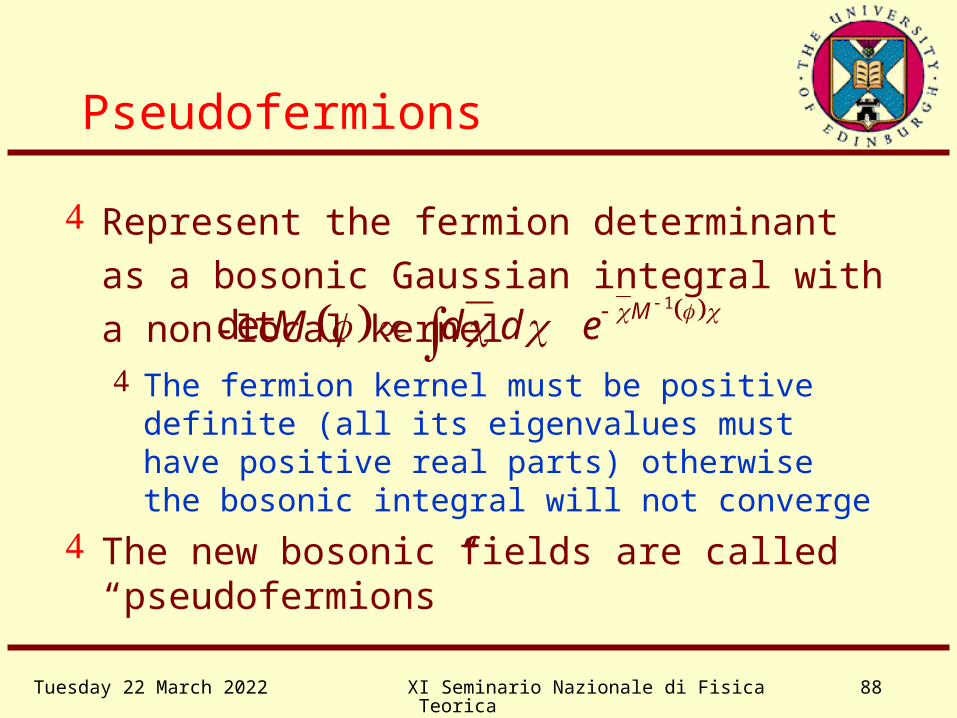
Pseudofermions
Represent the fermion determinant as a
bosonic Gaussian integral with a non-local
kernel 1
det MM d d e
The fermion kernel must be positive definite (all its eigenvalues must have positive real parts) otherwise the bosonic integral will not converge
The new bosonic fields are called “pseudofermions”

Wednesday 19 April 2023 XI Seminario Nazionale di Fisica Teorica 89
Pseudofermions
It is usually convenient to introduce two
flavours of fermion and to write
1†2 †det detM M
M M M d d e
This not only guarantees positivity, but also allows
us to generate the pseudofermions from a global heatbath by applying to a random Gaussian distributed field
†M

Wednesday 19 April 2023 XI Seminario Nazionale di Fisica Teorica 90
Equations of Motion
The evaluation of the pseudofermion action and the corresponding force then requires us to find the solution of a (large) set of linear equations 1†M M
The equations for motion for the boson (gauge) fields are and
†1 1† † †BS
M M M M M M
1† †BSM M

Wednesday 19 April 2023 XI Seminario Nazionale di Fisica Teorica 91
Linear Solver Accuracy
It is not necessary to carry out the inversions required for the equations of motion exactly There is a trade-off between the cost of computing
the force and the acceptance rate of the Metropolis MDMC step
The inversions required to compute the pseudofermion action for the accept/reject step does need to be computed exactly We usually take “exactly” to be synonymous with
“to machine precision”

Wednesday 19 April 2023 XI Seminario Nazionale di Fisica Teorica 92
Krylov Spaces
One of the main reasons why dynamical fermion lattice calculations are feasible is the existence of very effective numerical methods for solving large sparse systems of linear equations
Family of iterative methods based on Krylov spaces Conjugate Gradients (CG, CGNE) BiConjugate Gradients (BiCG, BiCGstab, BiCG5)

Wednesday 19 April 2023 XI Seminario Nazionale di Fisica Teorica 93
Krylov Spaces
These are often introduced as exact methods They require O(V) iterations to find the solution They do not give the exact answer in practice
because of rounding errors They are more naturally thought of as methods for
solving systems of linear equations in an (almost) -dimensional linear space
This is what we are approximating on the lattice anyway

Wednesday 19 April 2023 XI Seminario Nazionale di Fisica Teorica 94
BiCG on a Banach Space
We want to solve the equation Ax = b on a Banach space This is a normed linear space The norm endows the space with a topology The linear space operations are continuous in this
topology
We solve the system in the Krylov subspace
2 3span , , , , , nnK b Ab A b A b A b

Wednesday 19 April 2023 XI Seminario Nazionale di Fisica Teorica 95
BiCG on a Banach Space
There is no concept of “orthogonality” in a Banach space, so we also need to introduce a dual Krylov space of linear functionals on the Banach space
† †2 †3 †nˆ ˆ ˆ ˆ ˆˆ span , , , , ,nK b A b A b A b A b
The adjoint of a linear operator is defined by
† ˆ ˆA b x b Ax x
The vector is arbitraryb

Wednesday 19 April 2023 XI Seminario Nazionale di Fisica Teorica 96
BiCG on a Banach Space
We construct bi-orthonormal bases
0 1 1ˆ ˆ ˆ nR r r r 0 1 1nR r r r
0ˆr b0r b
† †1
ˆˆ ˆ ˆ1n nr RR A r †1
ˆ1n nr RR Ar
†R AR T
ˆnKnK
Galerkin condition (projectors)†ˆ 1R R Bi-orthogonality and normalisation
Lanczos tridiagonal formBiCGstab: minimise norm ||rn||
Short (3 term) recurrence

Wednesday 19 April 2023 XI Seminario Nazionale di Fisica Teorica 97
Tridiagonal Systems
The problem is now reduced to solving a fairly small tridiagonal system Hessenberg and Symmetric → Tridiagonal
= =

Wednesday 19 April 2023 XI Seminario Nazionale di Fisica Teorica 98
=
LU Decomposition
Reduce matrix to triangular form Gaussian elimination (LU decomposition)
11
11
1
11
11
1
11
11
1
11
11
1
=1
11
11
TL-1
U
1x A b
T LU1 1 1T U L
† † 1 † 10
ˆ ˆ ˆRR x RR A RR b RT e 1 10RU L e

Wednesday 19 April 2023 XI Seminario Nazionale di Fisica Teorica 99
11
1
QR Decomposition
Reduce matrix to triangular form Givens rotations (QR factorisation)
=11
1
1
11
11
1
= 11
1TQ-1
RT QR
1 1 1 1 †T R Q R Q

Wednesday 19 April 2023 XI Seminario Nazionale di Fisica Teorica 100
Krylov Solvers
Convergence is measured by the residualrn=||b – Axn|| Does not decrease monotonically for BiCG Better for BiCGstab Bad breakdown for unlucky choice of starting form LU might fail if zero pivot occurs QR is more stable
In a Hilbert space there is an inner product Which is relevant if A is symmetric (Hermitian) In this case we get the CG algorithm No bad breakdown (solution is in Krylov space) A>0 required only to avoid zero pivot for LU

Wednesday 19 April 2023 XI Seminario Nazionale di Fisica Teorica 101
Random Number Generators
Pseudorandom number generators Random numbers used infrequently in Monte
Carlo for QFT Compared to spin models
For suitable choice of a, b, and m (see, e.g., Donald Knuth, Art of Computer Programming)
Usually chose b = 0 and m = power of 2 Seem to be good enough in practice Problems for spin models if m is too small a multiple of V
Linear congruential generator 1 modn nx ax b m
Wednesday 19 April 2023 XI Seminario Nazionale di Fisica Teorica 102
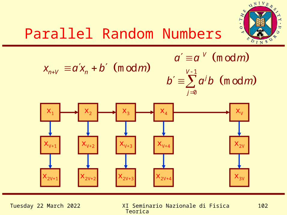
Parallel Random Numbers
1
0
mod
mod
V
Vj
j
a a m
b a b m
x1 x2 x3 x4 xV
xV+1 xV+2 xV+3 xV+4 x2V
x2V+1 x2V+2 x2V+3 x2V+4 x3V
mod n V nx a x b m

Wednesday 19 April 2023 XI Seminario Nazionale di Fisica Teorica 103
Acceptance Rates We can compute the average Metropolis
acceptance rate accP Area preservation implies that 1He
1 1 1H H H Hd d e d d e d d e eZ Z Z
The probability distribution of H has an asymptotic expansion
as the lattice volume V
2
1 1~ exp
44
HH
HP d d e H
Z HH
The average Metropolis acceptance rate is thus
21 1acc 2 8~ erfc erfcP H H
Wednesday 19 April 2023 XI Seminario Nazionale di Fisica Teorica 104
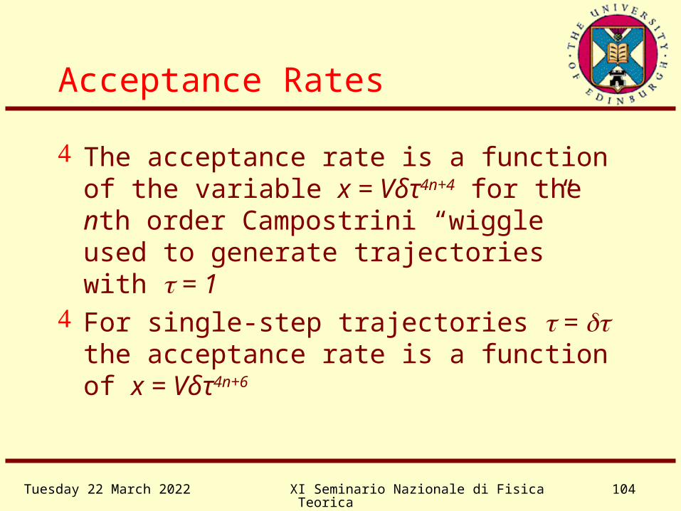
Acceptance Rates
The acceptance rate is a function of the variable x = Vδτ4n+4 for the nth order Campostrini “wiggle” used to generate trajectories with = 1
For single-step trajectories = the acceptance rate is a function of x = Vδτ4n+6

Wednesday 19 April 2023 XI Seminario Nazionale di Fisica Teorica 105
To a good approximation, the cost C of a Molecular Dynamics computation is proportional to the total time for which we have to integrate Hamilton’s equations.
Cost and Dynamical Critical Exponents
1 2C A
The cost per independent configuration is then
The optimal trajectory lengths obtained by minimising the cost as a function of the parameters , , and of the algorithm
Note that the cost depends on the particular operator under consideration

Wednesday 19 April 2023 XI Seminario Nazionale di Fisica Teorica 106
Cost and Dynamical Critical Exponents
While the cost depends upon the details of the implementation of the algorithm, the way that it scales with the correlation length of the system is an intrinsic property of the algorithm; where z is the dynamical critical exponent.
zC
For local algorithms the cost is independent of the trajectory length, , and thus minimising the cost is equivalent to minimising
1 2C A A
Free field theory analysis is useful for understanding and optimising algorithms, especially if our results do not depend on the details of the spectrum

Wednesday 19 April 2023 XI Seminario Nazionale di Fisica Teorica 107
Cost and Dynamical Critical Exponents
HMC For free field theory we can show that choosing
and = /2 gives z=1
This is to be compared with z=2 for constant
1/ 44 5 / 4/C V V V
The optimum cost for HMC is thus
For nth order Campostrini integration (if it were stable) the cost is
4 51
4 4 4 44 4 /n
n nnC V V V

Wednesday 19 April 2023 XI Seminario Nazionale di Fisica Teorica 108
Cost and Dynamical Critical Exponents
LMC For free field theory we can show that choosing
= and = /2 gives z=2
1/ 3 26 4 / 3 2/C V V V
The optimum cost for LMC is thus
For nth order Campostrini integration (if it were stable) the cost is
2 41
24 6 22 32 3 /n
n nnC V V V
Wednesday 19 April 2023 XI Seminario Nazionale di Fisica Teorica 109
Cost and Dynamical Critical Exponents
L2MC (Kramers)
In the approximation of unit acceptance rate we find that setting = and suitably tuning we can arrange to get z = 1
However, if then the system will carry out a random walk backwards and forwards along a trajectory because the momentum, and thus the direction of travel, must be reversed upon a Metropolis rejection.
acc 1P
Wednesday 19 April 2023 XI Seminario Nazionale di Fisica Teorica 110
A more careful free field theory analysis leads to the same conclusions
Cost and Dynamical Critical Exponents
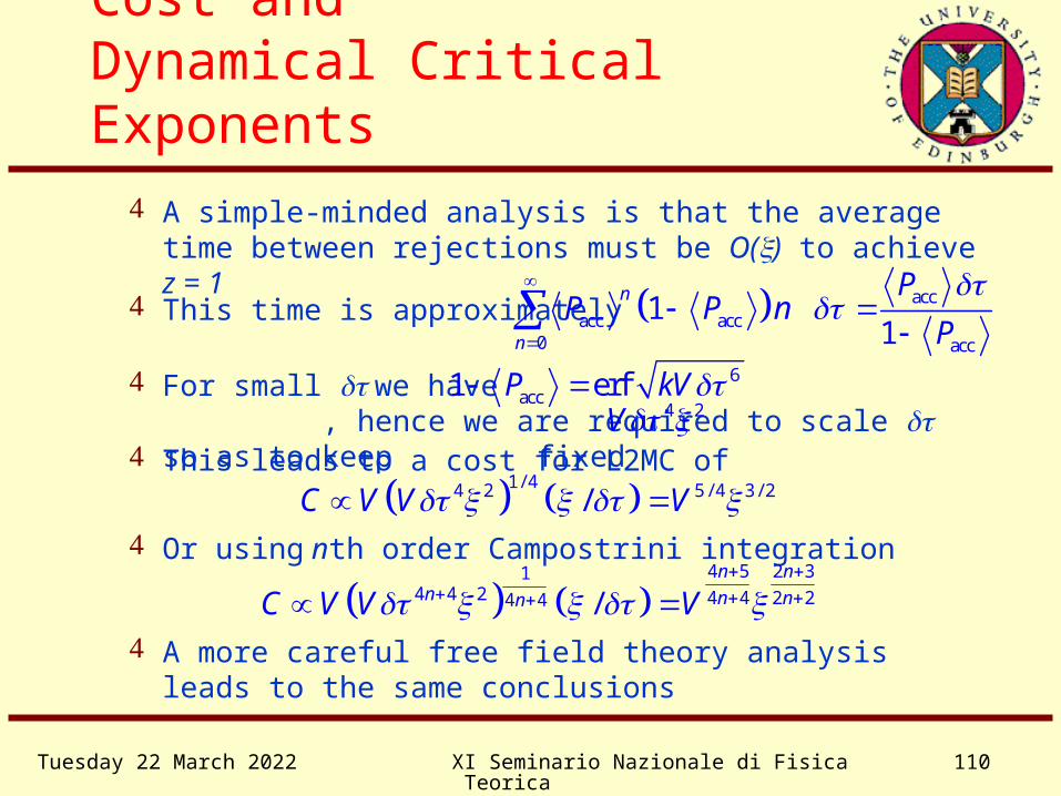
A simple-minded analysis is that the average time between rejections must be O() to achieve z = 1
This time is approximately accacc acc
0 acc
11
n
n
PP P n
P
For small we have , hence we are required to scale so as to keep fixed
6acc1 erfP kV
4 2V This leads to a cost for L2MC of
1/ 44 2 5 / 4 3 / 2/C V V V Or using nth order Campostrini integration
4 5 2 31
4 4 2 4 4 2 24 4 /n n
n n nnC V V V

Wednesday 19 April 2023 XI Seminario Nazionale di Fisica Teorica 111
Optimal parameters for GHMC (Almost) analytic
calculation in free field theory
Cost and Dynamical Critical Exponents
Minimum cost for GHMC appears for acceptance probability in the range 40%-90%
Very similar to HMC Minimum cost for L2MC
(Kramers) occurs for acceptance rate very close to 1
And this cost is much larger

Wednesday 19 April 2023 XI Seminario Nazionale di Fisica Teorica 112
Reversibility
Are HMC trajectories reversible and area preserving in practice? The only fundamental source of irreversibility is the rounding
error caused by using finite precision floating point arithmetic For fermionic systems we can also introduce irreversibility by
choosing the starting vector for the iterative linear equation solver time-asymmetrically
We might do this if we want to use (some extrapolation of) the previous solution as the starting vector
Floating point arithmetic is not associative It is more natural to store compact variables as scaled integers
(fixed point) Saves memory Does not solve the precision problem
Wednesday 19 April 2023 XI Seminario Nazionale di Fisica Teorica 113
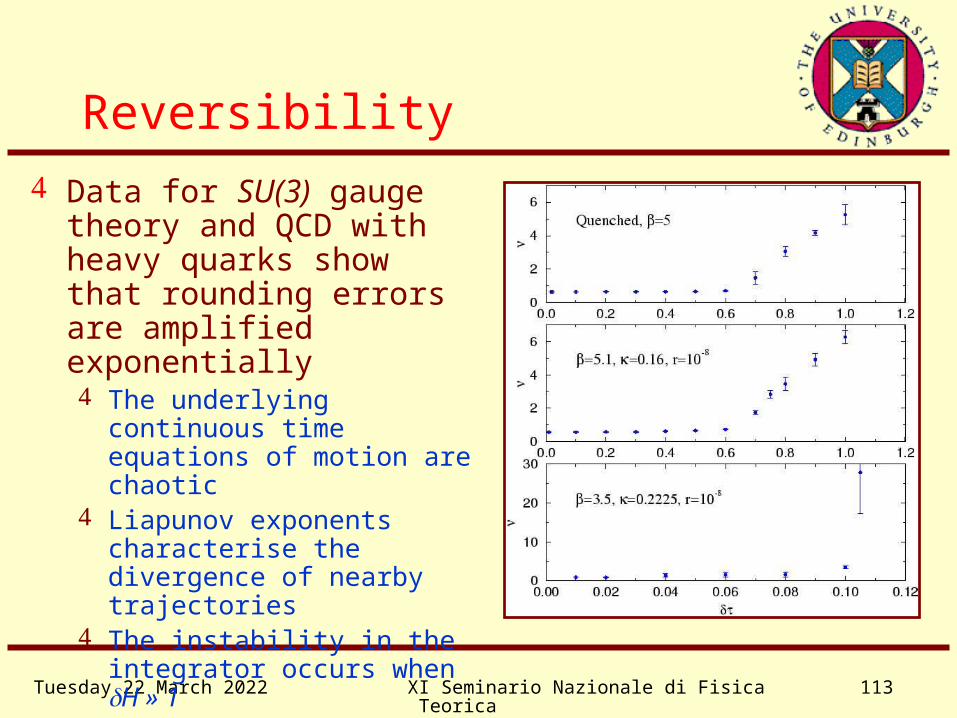
Reversibility
Data for SU(3) gauge theory and QCD with heavy quarks show that rounding errors are amplified exponentially The underlying continuous
time equations of motion are chaotic
Liapunov exponents characterise the divergence of nearby trajectories
The instability in the integrator occurs when H » 1
Zero acceptance rate anyhow

Wednesday 19 April 2023 XI Seminario Nazionale di Fisica Teorica 114
Reversibility
In QCD the Liapunov exponents appear to scalewith as the system approaches the continuum limit = constant This can be interpreted as saying that the Liapunov
exponent characterises the chaotic nature of the continuum classical equations of motion, and is not a lattice artefact
Therefore we should not have to worry about reversibility breaking down as we approach the continuum limit
Caveat: data is only for small lattices, and is not conclusive

Wednesday 19 April 2023 XI Seminario Nazionale di Fisica Teorica 115
0171.2,2.5,1355.0 lattice, 3216 SW3 c
Data for QCD with lighter dynamical quarks Instability occurs close to
region in where acceptance rate is near one
May be explained as a few “modes” becoming unstable because of large fermionic force
Integrator goes unstable if too poor an approximation to the fermionic force is used
Reversibility

Wednesday 19 April 2023 XI Seminario Nazionale di Fisica Teorica 116
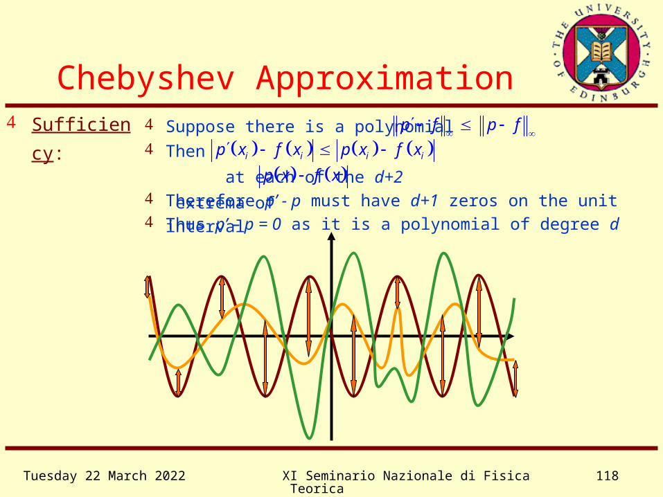
The error |p(x) - f(x)| reaches its maximum at exactly d+2 points on the unit interval
What is the best polynomial approximation p(x) to a continuous function f(x) for x in [0,1] ?
Chebyshev’s theorem
There is always a unique polynomial of any degree d which minimises
0 1max
xp f p x f x
Minimise the appropriate norm where n 1
11
0
nn
np f dx p x f x
Chebyshev Approximation
Weierstrass’ theorem: any continuous function can be arbitrarily well approximated by a polynomial
Bernstein polynomials: 0
(1 )n
n n kn
k
nkp x f t t
kn

Wednesday 19 April 2023 XI Seminario Nazionale di Fisica Teorica 117
Chebyshev Approximation Necessity: Suppose p-f has less than d+2 extrema of equal magnitude
Then at most d+1 maxima exceed some magnitude
We can construct a polynomial q of degree d which has the opposite sign to p-f at each of these maxima (Lagrange interpolation)
And whose magnitude is smaller than the “gap” The polynomial p+q is then a better approximation than p to f
This defines a “gap”
Wednesday 19 April 2023 XI Seminario Nazionale di Fisica Teorica 118
Chebyshev Approximation
Then at each of the d+2
extrema of
i i i ip x f x p x f x
p x f x
Thus p’ – p = 0 as it is a polynomial of degree d
Therefore p’ - p must have d+1 zeros on the unit interval
Sufficiency: Suppose there is a polynomial p f p f
Wednesday 19 April 2023 XI Seminario Nazionale di Fisica Teorica 119
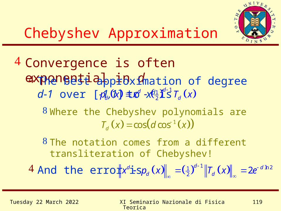
The notation comes from a different transliteration of Chebyshev!
Chebyshev Approximation
Convergence is often exponential in d The best approximation of degree d-1 over [-
1,1] to xd is 112
ddd dp x x T x
1cos cosdT x d x Where the Chebyshev polynomials are
1 ln 212 2
dd dd dx p x T x e
And the error is

Wednesday 19 April 2023 XI Seminario Nazionale di Fisica Teorica 120
Chebyshev Approximation
Chebyshev’s theorem is easily extended to rational approximations Rational functions with equal degree numerator
and denominator are usually best Convergence is still often exponential And rational functions usually give much better
approximations
Wednesday 19 April 2023 XI Seminario Nazionale di Fisica Teorica 121
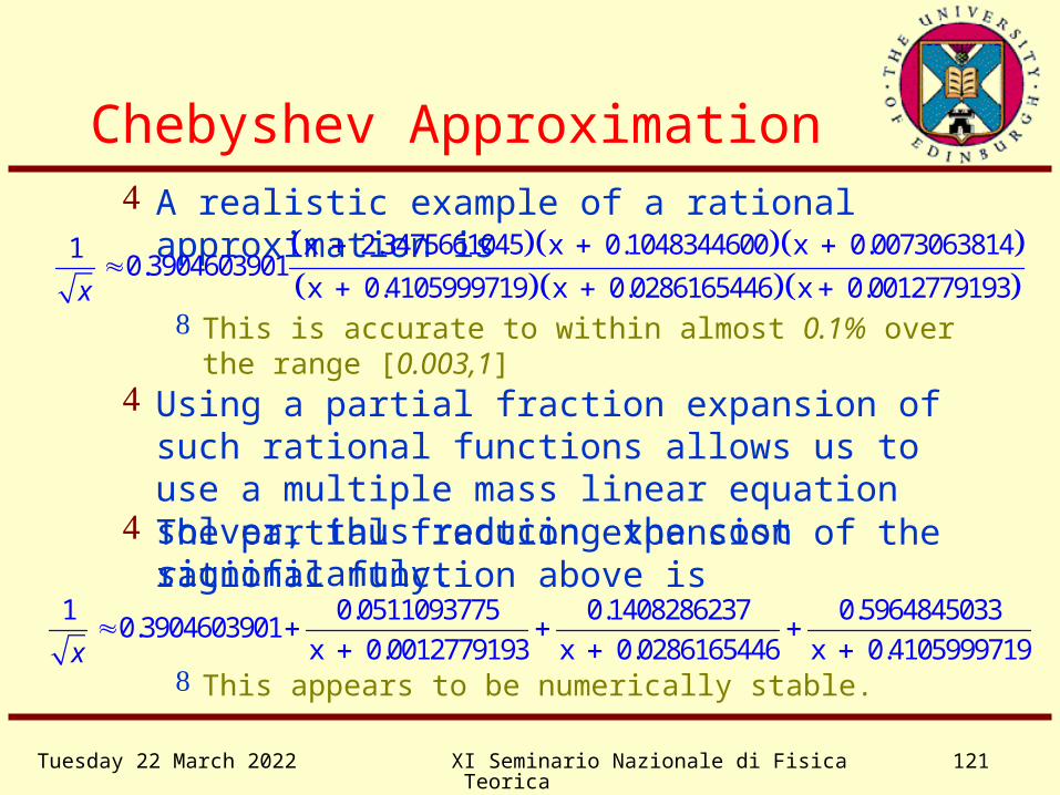
Chebyshev Approximation A realistic example of a rational approximation is
x 2.3475661045 x 0.1048344600 x 0.00730638141
0.3904603901x 0.4105999719 x 0.0286165446 x 0.0012779193x
Using a partial fraction expansion of such rational functions allows us to use a multiple mass linear equation solver, thus reducing the cost significantly.
1 0.0511093775 0.1408286237 0.59648450330.3904603901
x 0.0012779193 x 0.0286165446 x 0.4105999719x
The partial fraction expansion of the rational function above is
This is accurate to within almost 0.1% over the range [0.003,1]
This appears to be numerically stable.

Wednesday 19 April 2023 XI Seminario Nazionale di Fisica Teorica 122
Chebyshev Approximation

Wednesday 19 April 2023 XI Seminario Nazionale di Fisica Teorica 123
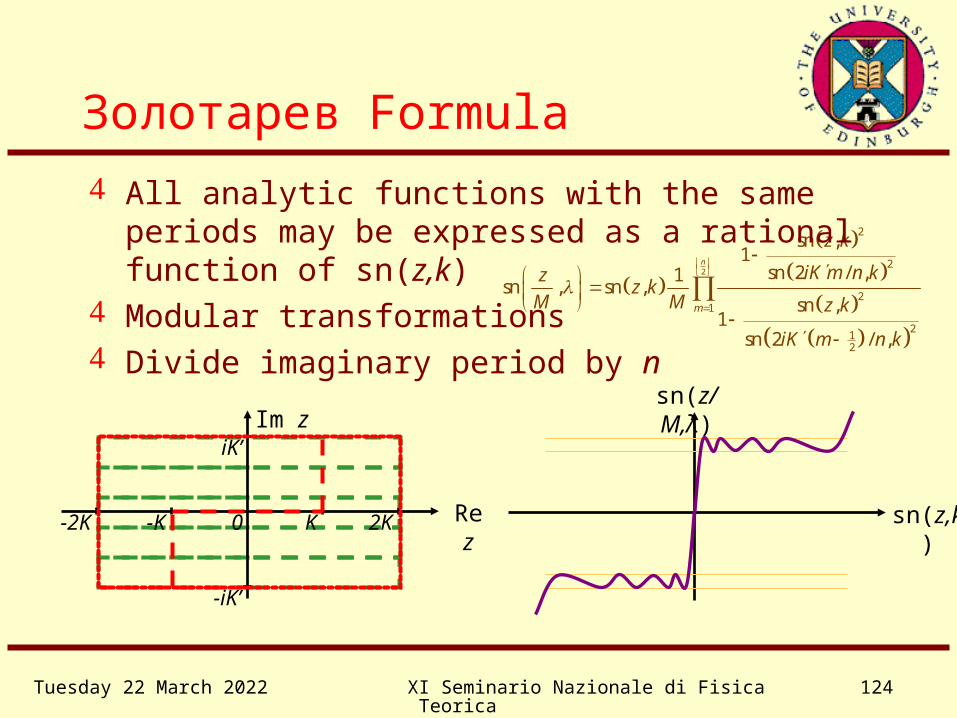
Золотарев Formula Elliptic function are doubly periodic analytic functions
Real period 4K, K=K(k) Imaginary period 2iK’, K’=K(k’) , k2+k’2=1
sn
2 2 20 1 1
z dtz
t k t
Jacobi elliptic function
1
2 2 20
K( )1 1
dtk
t k t
Complete elliptic integral
Im z
Re z0 2KK-2K -K
iK’
-iK’
∞1/k10-1
-1/k
Wednesday 19 April 2023 XI Seminario Nazionale di Fisica Teorica 124
Золотарев Formula
2
2
2
21
212
sn ,1
sn 2 / ,1sn , sn ,
sn ,1
sn 2 / ,
n
m
z k
iK m n kzz k
M M z k
iK m n k
Im z
Re z0 2KK-2K
-K
iK’
-iK’
All analytic functions with the same periods may be expressed as a rational function of sn(z,k)
Modular transformations Divide imaginary period by n
sn(z/M,λ)
sn(z,k)

Wednesday 19 April 2023 XI Seminario Nazionale di Fisica Teorica 125
Multibosons
1det i
i
M
det M 1det P M
1det i
i
M
†iM
ii
d e
Chebyshev polynomial approximations were introduced by Lüscher in his Multiboson method
No solution of linear equations is required One must store n scalar fields The dynamics of multiboson fields is stiff, so very
small step sizes are required for gauge field updates

Wednesday 19 April 2023 XI Seminario Nazionale di Fisica Teorica 126
Reweighting
Making Lüscher’s method exact One can introduce an accept/reject step One can reweight the configurations by the ratio
det[M] det[P(M)] This factor is close to one if P(M) is a good approximation If one only approximates 1/x over the interval [,1] which
does not cover the spectrum of M, then the reweighting factor may be large
It has been suggested that this will help to sample configurations which would otherwise be suppressed by small eigenvalues of the Dirac operator
Wednesday 19 April 2023 XI Seminario Nazionale di Fisica Teorica 127
Noisy methods
Since the GHMC algorithm is correct for any reversible and area-preserving mapping, it is often useful to use some modified MD process which is cheaper Accept/reject step must use the true Hamiltonian,
of course Tune the parameters in the MD Hamiltonian to
maximise the Metropolis acceptance rate Add irrelevant operators?
A different kind of “improvement”
Wednesday 19 April 2023 XI Seminario Nazionale di Fisica Teorica 128
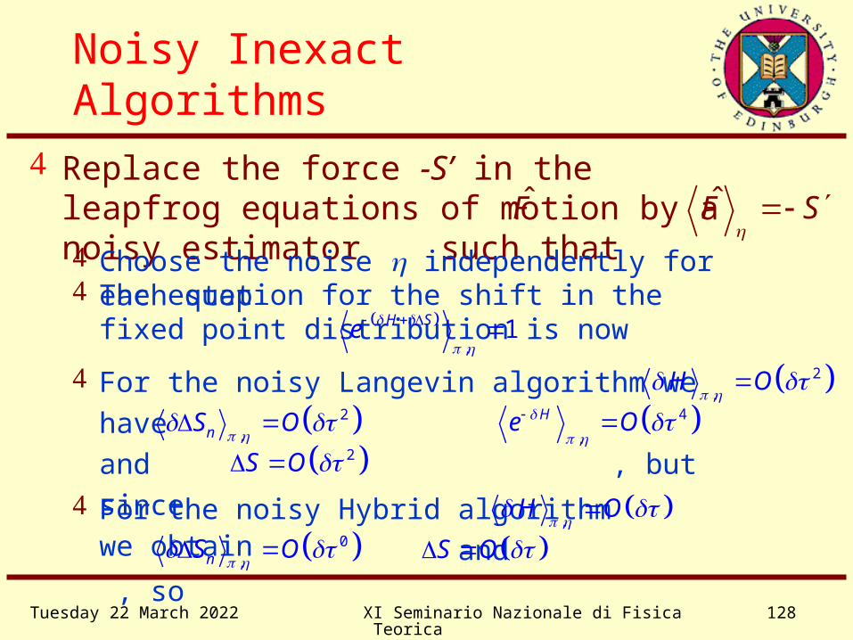
Noisy Inexact Algorithms Replace the force -S’ in the leapfrog equations
of motion by a noisy estimator such thatF F S
Choose the noise independently for each step The equation for the shift in the fixed point
distribution is now ,
1H Se
For the noisy Langevin algorithm we have
and , but since
we obtain
2
,H O
2
,nS O
4
,
He O
2S O
For the noisy Hybrid algorithm
and , so
,H O
0
,nS O
S O

Wednesday 19 April 2023 XI Seminario Nazionale di Fisica Teorica 129
Noisy Inexact Algorithms This method is useful for non-local actions, such as
staggered fermions with flavours 4fn Here the action may be written as , and the force is1
4 tr lnfn M 1trfn M M
A cheap way of estimating such a trace noisily is to use the fact that tr i ij jij
Q Q
One must use Gaussian noise (Z2 noise does not work)
Using a non area preserving irreversible update step the noisy Hybrid algorithm can be adjusted to have , and thus too
2
,H O
2S O This is the Hybrid R algorithm
Campostrini’s integration scheme may be used to produce higher order Langevin and Hybrid algorithms with for arbitrary n, but this is not applicable to the noisy versions
2nS O

Wednesday 19 April 2023 XI Seminario Nazionale di Fisica Teorica 130
If we look carefully at the proof that the Metropolis algorithm satisfies detailed balance we see that the ratio R is used for two quite different purposes It is used to give an ordering to configurations: ’ < if R < 1, that is,
if Q(’) < Q() It is used as the acceptance probability if ’ <
Kennedy—Kuti Algorithm Suppose it is prohibitively expensive to evaluate ,
but that we can compute an unbiased estimator for it cheaply, R Q Q
R R
A suitable ordering is provided by any “cheap” function f such that the set of configurations for which f(’) = f() has measure zero
We can produce a valid algorithm using the noisy estimator for the latter rôle just by choosing another ordering for the configurations
R
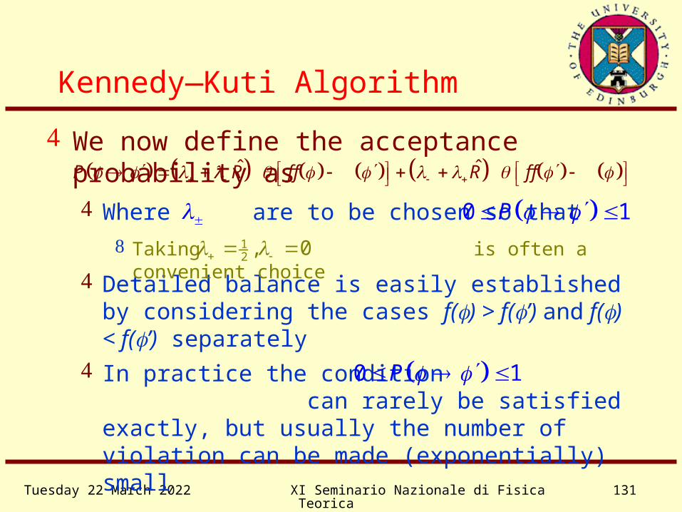
Wednesday 19 April 2023 XI Seminario Nazionale di Fisica Teorica 131
Detailed balance is easily established by considering the cases f() > f(’) and f() < f(’) separately
Kennedy—Kuti Algorithm
We now define the acceptance probability as ˆ ˆP R f f R f f
Taking is often a convenient choice12 , 0
Where are to be chosen so that 0 1P
In practice the condition can rarely be satisfied exactly, but usually the number of violation can be made (exponentially) small
0 1P
Wednesday 19 April 2023 XI Seminario Nazionale di Fisica Teorica 132
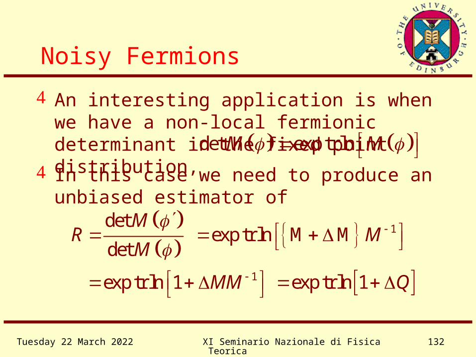
Noisy Fermions
det
det
MR
M
In this case we need to produce an unbiased estimator of
1exp tr ln 1 MM
1exp tr ln M M M
exp tr ln 1 Q
An interesting application is when we have a non-local fermionic determinant in the fixed point distribution, det exp tr lnM M
Wednesday 19 April 2023 XI Seminario Nazionale di Fisica Teorica 133
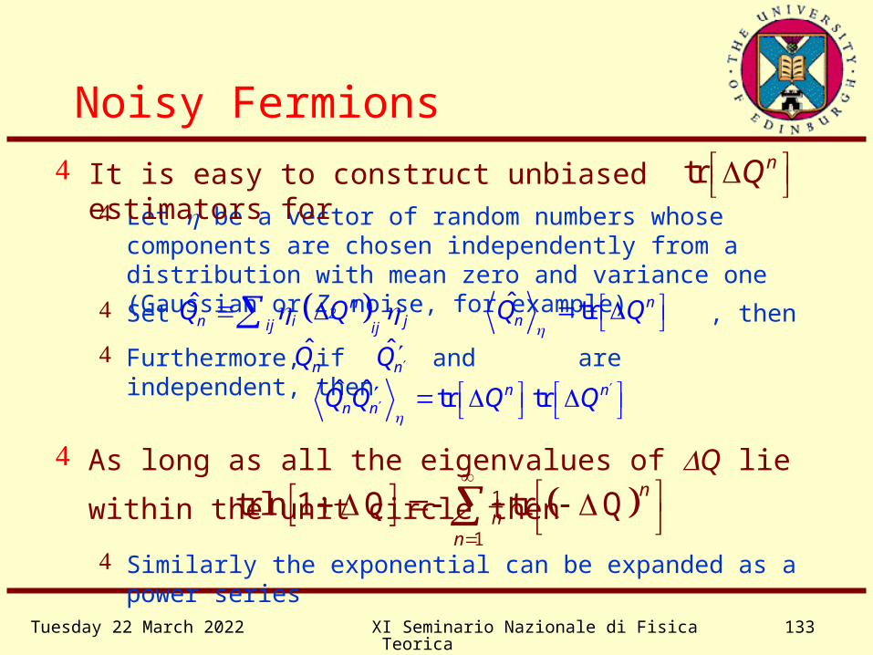
As long as all the eigenvalues of Q lie within the unit
circle then 1
1
tr ln 1 Q tr Qn
nn
Noisy Fermions
Let be a vector of random numbers whose components are chosen independently from a distribution with mean zero and variance one (Gaussian or Z2 noise, for example)
It is easy to construct unbiased estimators for tr nQ
Set , then ˆ nn i jij ij
Q Q ˆ tr nnQ Q
Furthermore, if and are independent, thenˆnQ ˆ
nQ ˆ ˆ tr trn n
n nQ Q Q Q
Similarly the exponential can be expanded as a power series
Wednesday 19 April 2023 XI Seminario Nazionale di Fisica Teorica 134
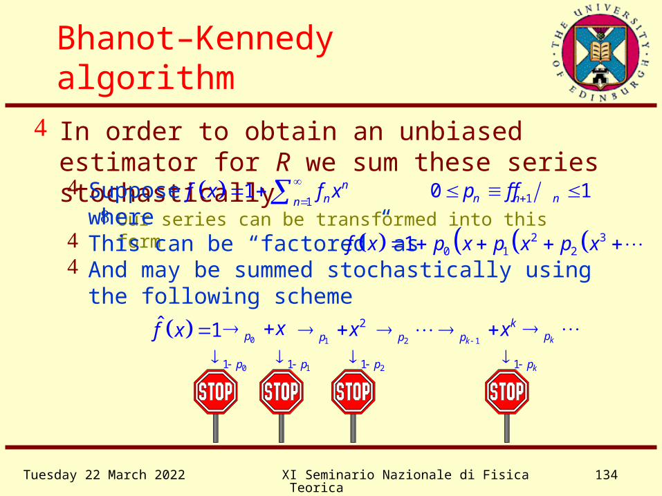
Bhanot–Kennedy algorithm
In order to obtain an unbiased estimator for R we sum these series stochastically
Our series can be transformed into this form
Suppose where 1
1 nnn
f x f x
10 1n n np f f
And may be summed stochastically using the following scheme
This can be “factored” as 2 30 1 21f x p x p x p x
ˆ 1f x 0p x
1
2p x
2 1k
kp p x
kp
01 p11 p
21 p 1 kp

Wednesday 19 April 2023 XI Seminario Nazionale di Fisica Teorica 135
This gets rid of the systematic errors of the Kennedy—Kuti method by eliminating the violations
“Kentucky” Algorithm
Promote the noise to the status of dynamical fields
1detSd e M
Z 1 ˆ ,Sd e R
Z
1 ˆ ,Sd d e p RZ
1 ˆ ˆ, sgn ,Sd d e p R R
Z
,
ˆsgn ,R
ˆ ˆ, , detR d p R M
Suppose that we have an unbiased estimator

Wednesday 19 April 2023 XI Seminario Nazionale di Fisica Teorica 136
“Kentucky” Algorithm
The and fields can be updated by alternating Metropolis Markov steps
There is a sign problem only if the Kennedy—Kuti algorithm would have many violations
If one constructs the estimator using the Kennedy—Bhanot algorithm then one will need an infinite number of noise fields in principle Will these ever reach equilibrium?

Wednesday 19 April 2023 XI Seminario Nazionale di Fisica Teorica 137
Cost of Noisy Algorithms
Inexact algorithms These have only a trivial linear volume dependence,
with z = 1 for Hybrid and z = 2 for Langevin
Noisy inexact algorithms The noisy trajectories deviate from the true classical
trajectory by a factor of for each step, or for a trajectory of steps
1 O 1 O
This will not affect the integrated autocorrelation function as long as «1
2C V V Thus the noisy Hybrid algorithm should have
Thus the noisy Langevin algorithm should have 2C V

Wednesday 19 April 2023 XI Seminario Nazionale di Fisica Teorica 138
Cost of Noisy Algorithms
Noisy exact algorithms These algorithms use noisy estimators to produce
an (almost) exact algorithm which is applicable to non-local actions
2C V V V An exact noisy Hybrid algorithm is also possible, and for it
It is amusing to note that this algorithm should not care what force term is used in the equations of motion
A straightforward approach leads to a cost of
for exact noisy
Langevin 22 2 2C V V V

Wednesday 19 April 2023 XI Seminario Nazionale di Fisica Teorica 139
Cost of Noisy Algorithms
These results apply only to operators (like the magnetisation) which couple sufficiently strongly to the slowest modes of the system. For other operators, like the energy in 2 dimensions, we can even obtain z = 0
Wednesday 19 April 2023 XI Seminario Nazionale di Fisica Teorica 140
Cost of Noisy Algorithms
Summary Too little noise increases critical slowing down
because the system is too weakly ergodic Too much noise increases critical slowing down
because the system takes a drunkard’s walk through phase space
To attain z = 1 for any operator (and especially for the exponential autocorrelation time) one must be able to tune the amount of noise suitably
Wednesday 19 April 2023 XI Seminario Nazionale di Fisica Teorica 141
PHMC
Polynomial Hybrid Monte Carlo algorithm Instead of using Chebyshev polynomials in the multiboson
algorithm, Frezzotti & Jansen and deForcrand suggested using them directly in HMC
Polynomial approximation to 1/x are typically of order 40 to 100 at present
Numerical stability problems with high order polynomial evaluation
Polynomials must be factored Correct ordering of the roots is important Frezzotti & Jansen claim there are advantages from using
reweighting
Wednesday 19 April 2023 XI Seminario Nazionale di Fisica Teorica 142
RHMC
Rational Hybrid Monte Carlo algorithm The idea is similar to PHMC, but uses rational
approximations instead of polynomial ones Much lower orders required for a given accuracy Evaluation simplified by using partial fraction
expansion and multiple mass linear equation solvers
1/x is already a rational function, so RHMC reduces to HMC in this case
Can be made exact using noisy accept/reject step
Wednesday 19 April 2023 XI Seminario Nazionale di Fisica Teorica 143
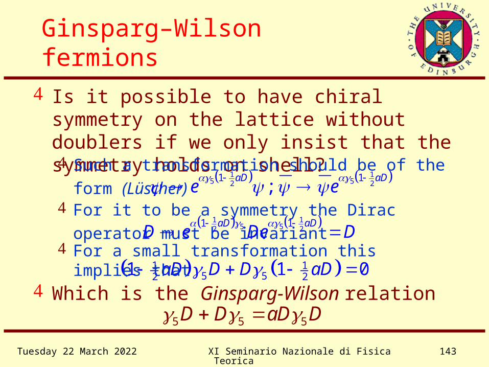
Is it possible to have chiral symmetry on the lattice without doublers if we only insist that the symmetry holds on shell?
Ginsparg–Wilson fermions
Such a transformation should be of the form
(Lüscher) 1 1
5 52 21 1
;aD aD
e e
For it to be a symmetry the Dirac operator must be
invariant 1 1
5 52 21 1aD aD
D e De D
1 15 52 21 1 0aD D D aD
For a small transformation this implies that
5 5 5D D aD D Which is the Ginsparg-Wilson relation
Wednesday 19 April 2023 XI Seminario Nazionale di Fisica Teorica 144
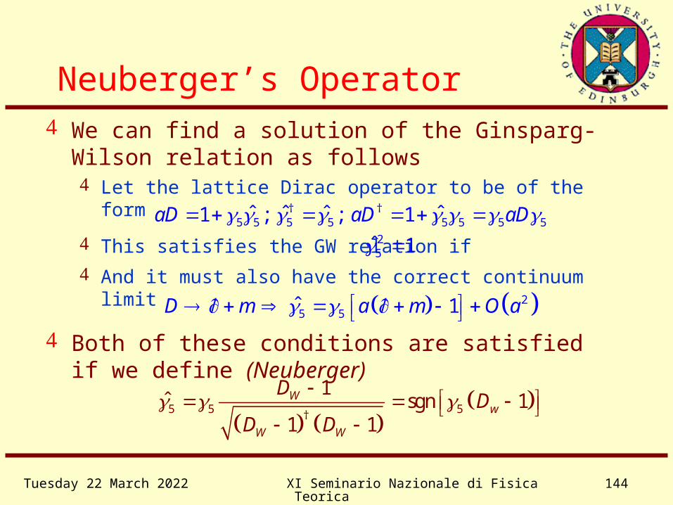
Neuberger’s Operator We can find a solution of the Ginsparg-Wilson relation
as follows
† †5 5 5 5 5 5 5 5ˆ ˆ ˆ ˆ1 ; ; 1aD aD aD
Let the lattice Dirac operator to be of the form
This satisfies the GW relation if 25ˆ 1
25 5ˆ 1D m a m O a
And it must also have the correct continuum limit
5 5 5†
1ˆ sgn 1
1 1
Ww
W W
DD
D D
Both of these conditions are satisfied if we define (Neuberger)
Wednesday 19 April 2023 XI Seminario Nazionale di Fisica Teorica 145
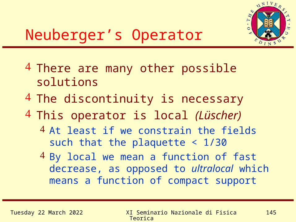
Neuberger’s Operator
There are many other possible solutions The discontinuity is necessary This operator is local (Lüscher)
At least if we constrain the fields such that the plaquette < 1/30
By local we mean a function of fast decrease, as opposed to ultralocal which means a function of compact support

Wednesday 19 April 2023 XI Seminario Nazionale di Fisica Teorica 146
ComputingNeuberger’s Operator
Use polynomial approximation to Neuberger’s operator High degree polynomials have numerical instabilities For dynamical GW fermions this leads to a PHMC algorithm
Use rational approximation Optimal rational approximations for sgn(x) are know in closed form
(Zolotarev) Requires solution of linear equations just to apply the operator For dynamical GW fermions this leads to an RHMC algorithm Requires nested linear equation solvers in the dynamical case Nested solvers can be avoided at the price of a much more ill-
conditioned system Attempts to combine inner and outer solves in one Krylov space
method

Wednesday 19 April 2023 XI Seminario Nazionale di Fisica Teorica 147
ComputingNeuberger’s Operator
Extract low-lying eigenvectors explicitly, and evaluate their contribution to the Dirac operator directly Efficient methods based on Ritz functional Very costly for dynamical fermions if there is a finite density
of zero eigenvalues in the continuum limit (Banks—Casher) Might allow for noisy accept/reject step if we can replace the
step function with something continuous (so it has a reasonable series expansion)
Use better approximate solution of GW relation instead of Wilson operator E.g., a relatively cheap “perfect action”

Wednesday 19 April 2023 XI Seminario Nazionale di Fisica Teorica 148
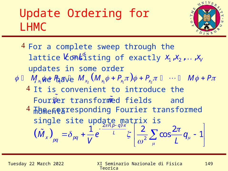
Update Ordering for LHMC Consider the update of a single site x using the
LHMC algorithm
2
21
Fx x
This may be written in matrix form as where
x xM P
ˆ ˆ, ,2
1x yz xy yz y z y zyz
M
2
x yz xyyzP
The values of at all other sites are left unchanged
Wednesday 19 April 2023 XI Seminario Nazionale di Fisica Teorica 149
Update Ordering for LHMC
For a complete sweep through the lattice consisting
of exactly updates in some order ,
we have
dV L 1 2, , , Vx x x
1 1 2 1 1 2x x x x x xM P M M P P M P
It is convenient to introduce the Fourier transformed
fields and momenta
2
2
1 2 2cos 1
i p q x
Lx pqpq
M e qV L
The corresponding Fourier transformed single site
update matrix is

Wednesday 19 April 2023 XI Seminario Nazionale di Fisica Teorica 150
Update Ordering for LHMC We want to compute integrated autocorrelation
functions for operators like the magnetic
susceptibility
2 20 0
The behaviour of the autocorrelations of linear operators such as
the magnetisation can be misleading0 In order to do this it is useful to consider quadratic operators
as linear operators on quadratic monomials in the fields,
, sopq p q
00 00
Where and ,Qpq rs pr qsM M MQ
pq pr qrr
P P P
pq p q p qM P M P
These quadratic monomials are updated according to
Q QM P
So, after averaging over the momenta we have

Wednesday 19 April 2023 XI Seminario Nazionale di Fisica Teorica 151
Update Ordering for LHMC
20 0
01
t t
tA C t
00 0000,
220
00 00
tQpq pqpq
pq
t
M
1
00,000 00,00
1tQ Q
t
M M
The integrated autocorrelation function for is

Wednesday 19 April 2023 XI Seminario Nazionale di Fisica Teorica 152
Update Ordering for LHMC
The update matrix for a sweep after averaging over the V independent choices of update sites is just
1 11
1 1i
i
VV V V
Q Q Qz z
z zi
M M MV V
Random updates
2
2
2
2
1 1
1m
m d
OV
e
02
1dO m O
Vm
1
00,00
1 QM
Which tells us that z = 2 for any choice of the overrelaxation parameter
We thus find that 1 A

Wednesday 19 April 2023 XI Seminario Nazionale di Fisica Teorica 153
Update Ordering for LHMC
The update matrix for a sweep in Fourier space thus reduces to a 2 × 2 matrix coupling and p 1
2, ,p L L
thus becomes a 3 × 3 matrix in this caseQM
Even/Odd updates In a single site update the new value of the field at x only
depends at the old value at x and its nearest neighbours, so even sites depend only on odd sites and vice versa
24
2
2 7 16 8
9 22
dA O m
m
The integrated autocorrelation function is
1
2
dA O m
m
22m
O md
This is minimised by choosing , for which
Hence z = 1

Wednesday 19 April 2023 XI Seminario Nazionale di Fisica Teorica 154
new
old
updateable
A single site update depends on the new values of the neighbouring sites in the + directions and the old values in the - directions
Except at the edges of the lattice
Update Ordering for LHMC
This is a scheme in which is always updated beforeˆx x
So we may write the sweep update implicitly as O N P
ˆ,2
11xy xy x y xyO R
L
ˆ ˆ, 1 ,2xy x y x x y x L
LR
2
P
Lexicographical updates
Where
ˆ,2
1xy x y xyN R
L

Wednesday 19 April 2023 XI Seminario Nazionale di Fisica Teorica 155
Update Ordering for LHMC
The Fourier transforms and are diagonal up to surface terms , which we expect to be suppressed by a factor of 1/L
O NR
11M N O
11P N P
The sweep update matrices are easily found explicitly
22
2 2
2 11
2 2
m dA O
Lm m d
We thus obtain
2
2
2m d
m d
Which is minimised by the choice
For which and hence z = 00A This can be achieved for most operators
Though with different values of The dynamical critical exponent for the exponential
autocorrelation time is still one at best