An Introduction to MATLAB for Geoscientists
140
An Introduction to MATLAB for Geoscientists Dave Heslop Version: January 2010
Transcript of An Introduction to MATLAB for Geoscientists
An Introduction to MATLAB for Geoscientists
Dave Heslop
Version: January 2010

Contents
1 Introduction 41.1 MATLAB . . . . . . . . . . . . . . . . . . . . . . . . . . . . . . . . . . . . . . . 4
1.1.1 Obtaining a copy of MATLAB . . . . . . . . . . . . . . . . . . . . . . . . 41.1.2 Useful MATLAB books . . . . . . . . . . . . . . . . . . . . . . . . . . . . 51.1.3 Everyday help with MATLAB . . . . . . . . . . . . . . . . . . . . . . . . 51.1.4 How these notes are structured . . . . . . . . . . . . . . . . . . . . . . . 5
1.2 Getting started . . . . . . . . . . . . . . . . . . . . . . . . . . . . . . . . . . . . 61.2.1 The Command Window . . . . . . . . . . . . . . . . . . . . . . . . . . . 61.2.2 The Command History . . . . . . . . . . . . . . . . . . . . . . . . . . . . 61.2.3 Workspace . . . . . . . . . . . . . . . . . . . . . . . . . . . . . . . . . . . 71.2.4 The Current Directory setting . . . . . . . . . . . . . . . . . . . . . . . . 8
2 Simple operations and working with variables 92.1 Using variables; scalars, vectors and matrices . . . . . . . . . . . . . . . . . . . . 9
2.1.1 Simple scalar arithmetic . . . . . . . . . . . . . . . . . . . . . . . . . . . 92.1.2 Order of evaluation . . . . . . . . . . . . . . . . . . . . . . . . . . . . . . 102.1.3 Using named variables . . . . . . . . . . . . . . . . . . . . . . . . . . . . 122.1.4 Rules for naming variables . . . . . . . . . . . . . . . . . . . . . . . . . . 152.1.5 Navigating the Command History and updating variables . . . . . . . . . 152.1.6 Simple Arrays . . . . . . . . . . . . . . . . . . . . . . . . . . . . . . . . . 172.1.7 Array-Scalar and Array-Array Arithmetic . . . . . . . . . . . . . . . . . 21
3 MATLAB Functions 243.1 Script M-files and the MATLAB Editor . . . . . . . . . . . . . . . . . . . . . . . 243.2 Working with “inbuilt” functions . . . . . . . . . . . . . . . . . . . . . . . . . . 25
3.2.1 Taking the square root . . . . . . . . . . . . . . . . . . . . . . . . . . . . 253.2.2 The help command . . . . . . . . . . . . . . . . . . . . . . . . . . . . . . 263.2.3 Finding the right function . . . . . . . . . . . . . . . . . . . . . . . . . . 273.2.4 Multiple inputs and outputs . . . . . . . . . . . . . . . . . . . . . . . . . 28
3.3 Exercise: Mmmm, π . . . . . . . . . . . . . . . . . . . . . . . . . . . . . . . . . 293.4 Writing your own functions . . . . . . . . . . . . . . . . . . . . . . . . . . . . . 31
3.4.1 Inline functions . . . . . . . . . . . . . . . . . . . . . . . . . . . . . . . . 313.4.2 M-functions . . . . . . . . . . . . . . . . . . . . . . . . . . . . . . . . . . 32
3.5 Exercise: Mmmm, a second helping of π . . . . . . . . . . . . . . . . . . . . . . 363.6 Exercise: The Geiger counter . . . . . . . . . . . . . . . . . . . . . . . . . . . . 37
1

4 Relational and logical operators 394.1 Relational and logical operations . . . . . . . . . . . . . . . . . . . . . . . . . . 39
4.1.1 Relational testing . . . . . . . . . . . . . . . . . . . . . . . . . . . . . . . 394.1.2 Logical Operators . . . . . . . . . . . . . . . . . . . . . . . . . . . . . . . 424.1.3 Controlling the flow of your code . . . . . . . . . . . . . . . . . . . . . . 434.1.4 For Loops . . . . . . . . . . . . . . . . . . . . . . . . . . . . . . . . . . . 44
4.2 Exercise 1: Classifying sediments . . . . . . . . . . . . . . . . . . . . . . . . . . 464.3 Exercise 2: The Safe Cracker . . . . . . . . . . . . . . . . . . . . . . . . . . . . . 47
4.3.1 An even worse safe . . . . . . . . . . . . . . . . . . . . . . . . . . . . . . 49
5 Input / Output and data management 515.1 Import . . . . . . . . . . . . . . . . . . . . . . . . . . . . . . . . . . . . . . . . . 51
5.1.1 Copy and Paste . . . . . . . . . . . . . . . . . . . . . . . . . . . . . . . . 515.1.2 The load function . . . . . . . . . . . . . . . . . . . . . . . . . . . . . . 535.1.3 Low-level I/O functions . . . . . . . . . . . . . . . . . . . . . . . . . . . 555.1.4 Import from an EXCEL workbook . . . . . . . . . . . . . . . . . . . . . 565.1.5 NetCDF files . . . . . . . . . . . . . . . . . . . . . . . . . . . . . . . . . 57
5.2 Export . . . . . . . . . . . . . . . . . . . . . . . . . . . . . . . . . . . . . . . . . 575.2.1 Outputting a simple ASCII file . . . . . . . . . . . . . . . . . . . . . . . 575.2.2 Exporting to an EXCEL workbook . . . . . . . . . . . . . . . . . . . . . 585.2.3 Writing formatted text files . . . . . . . . . . . . . . . . . . . . . . . . . 59
5.3 Data Management . . . . . . . . . . . . . . . . . . . . . . . . . . . . . . . . . . 605.4 Exercise: Entering data into a structural array . . . . . . . . . . . . . . . . . . . 62
6 Plotting in two-dimensions 636.1 Plotting in two-dimensions . . . . . . . . . . . . . . . . . . . . . . . . . . . . . . 63
6.1.1 Figure windows . . . . . . . . . . . . . . . . . . . . . . . . . . . . . . . . 636.1.2 Using Handles . . . . . . . . . . . . . . . . . . . . . . . . . . . . . . . . . 64
6.2 Simple data plotting . . . . . . . . . . . . . . . . . . . . . . . . . . . . . . . . . 646.2.1 Modifying the axes . . . . . . . . . . . . . . . . . . . . . . . . . . . . . . 676.2.2 Multiple sets of axes in a single figure . . . . . . . . . . . . . . . . . . . . 686.2.3 Different types of plots . . . . . . . . . . . . . . . . . . . . . . . . . . . . 706.2.4 Contour plots . . . . . . . . . . . . . . . . . . . . . . . . . . . . . . . . . 716.2.5 Saving and exporting figures . . . . . . . . . . . . . . . . . . . . . . . . . 75
6.3 Exercise: Life’s ups and downs in the Logistic Map . . . . . . . . . . . . . . . . 75
7 Plotting in three-dimensions 817.1 Plotting in three-dimensions . . . . . . . . . . . . . . . . . . . . . . . . . . . . . 81
7.1.1 Plotting points and lines . . . . . . . . . . . . . . . . . . . . . . . . . . . 827.1.2 Surface plots . . . . . . . . . . . . . . . . . . . . . . . . . . . . . . . . . 847.1.3 Overlaying images . . . . . . . . . . . . . . . . . . . . . . . . . . . . . . 86
7.2 Exercise: Plotting elevation data . . . . . . . . . . . . . . . . . . . . . . . . . . 88
8 Interpolation 908.1 Interpolation in one dimension . . . . . . . . . . . . . . . . . . . . . . . . . . . . 90
8.1.1 Piecewise Linear Interpolation . . . . . . . . . . . . . . . . . . . . . . . . 928.1.2 Nearest Neighbor Interpolation . . . . . . . . . . . . . . . . . . . . . . . 94
2

8.1.3 Cubic spline Interpolation . . . . . . . . . . . . . . . . . . . . . . . . . . 958.1.4 PCHIP Interpolation . . . . . . . . . . . . . . . . . . . . . . . . . . . . . 96
8.2 The dangers of extrapolation . . . . . . . . . . . . . . . . . . . . . . . . . . . . . 978.3 Interpolation in two dimensions . . . . . . . . . . . . . . . . . . . . . . . . . . . 988.4 Interpolation in higher dimensions . . . . . . . . . . . . . . . . . . . . . . . . . . 101
9 Optimization 1029.1 Minimization in one dimension . . . . . . . . . . . . . . . . . . . . . . . . . . . . 102
9.1.1 How does it work? . . . . . . . . . . . . . . . . . . . . . . . . . . . . . . 1049.2 Minimization in higher dimensions . . . . . . . . . . . . . . . . . . . . . . . . . 1079.3 Constrained Optimization . . . . . . . . . . . . . . . . . . . . . . . . . . . . . . 110
9.3.1 Linear Equalities . . . . . . . . . . . . . . . . . . . . . . . . . . . . . . . 1129.3.2 Linear inequalities . . . . . . . . . . . . . . . . . . . . . . . . . . . . . . 114
9.4 Exercise: The Geiger counter . . . . . . . . . . . . . . . . . . . . . . . . . . . . 115
10 Final Project 11710.1 Sand, Silt and Clay in an Arctic Lake . . . . . . . . . . . . . . . . . . . . . . . . 117
10.1.1 Importing the data . . . . . . . . . . . . . . . . . . . . . . . . . . . . . . 11710.1.2 Plotting the data . . . . . . . . . . . . . . . . . . . . . . . . . . . . . . . 11710.1.3 Define a regression relationship . . . . . . . . . . . . . . . . . . . . . . . 11810.1.4 Plot the regression relationship . . . . . . . . . . . . . . . . . . . . . . . 119
10.2 Exercise: Bringing it all together with cars and goats . . . . . . . . . . . . . . . 120
11 Exercise Solutions 12311.1 Solution: Mmmm, π . . . . . . . . . . . . . . . . . . . . . . . . . . . . . . . . . 123
11.1.1 Golf Solution: Mmmm, π . . . . . . . . . . . . . . . . . . . . . . . . . . 12411.2 Solution: Mmmm, a second helping of π . . . . . . . . . . . . . . . . . . . . . . 12411.3 Solution: The Geiger counter . . . . . . . . . . . . . . . . . . . . . . . . . . . . 12511.4 Solution: Classifying sediments . . . . . . . . . . . . . . . . . . . . . . . . . . . 12811.5 Solution: The Safe Cracker . . . . . . . . . . . . . . . . . . . . . . . . . . . . . . 12911.6 Solution: An even worse safe . . . . . . . . . . . . . . . . . . . . . . . . . . . . . 13111.7 Solution: Life’s ups and downs in the Logistic Map . . . . . . . . . . . . . . . . 13311.8 Solution: Plotting elevation data . . . . . . . . . . . . . . . . . . . . . . . . . . 13411.9 Solution: The Geiger counter . . . . . . . . . . . . . . . . . . . . . . . . . . . . 13511.10Solution: Sand, Silt and Clay in an Arctic Lake . . . . . . . . . . . . . . . . . . 13511.11Solution: Bringing it all together with cars and goats . . . . . . . . . . . . . . . 137
3

Chapter 1
Introduction
1.1 MATLAB
MATLAB, short for Matrix Laboratory, is a numerical computing environment and programminglanguage originally developed by Cleve Moler. Evolving dramatically from its first release,MATLAB is now over 30 years old and is distributed commercially by The MathWorks Inc. Inthis course we will work through a number examples which are designed to help you come toterms with the basics of MATLAB and see how you can use it in your own research. BecauseMATLAB is programmable it provides an environment in which we can process scientific datawithout the need to use specific software packages which are limited in the tasks they canperform. The three main advantages of using MATLAB for your day-to-day scientific work are:
• It is an interpreted language, this means we can work step by step through a series ofcommands without the need for compiling complete sets of code.
• MATLAB is based around so-called “inbuilt” functions which provide quick access tothousands of different data processing methods.
• MATLAB contains versatile graphics libraries allowing you to view your data in a varietyof ways as it is processed.
One of the first things you’ll notice about MATLAB is that it is command driven. If you arenormally working with EXCEL you probably spend 95% of your time using the mouse andonly 5% typing on the keyboard. In MATLAB the opposite is true and whilst this might seemannoying at first, you’ll hopefully soon come to recognize why this is necessary.
1.1.1 Obtaining a copy of MATLAB
In its distribution of MATLAB The MathWorks promotes the a system based around “tool-boxes”. This means that MATLAB by itself is relatively cheap, but if you want to performspecialist tasks such as statistics, image processing or optimization you can also buy specifictoolboxes which greatly enhance the methods available to you. Currently there are over fiftydifferent toolboxes available for tasks as diverse as modelling biological systems to fuzzy logicand you have to pay about 400 euros for each one you use. Overall this means MATLAB can bevery expensive once you add on a number of toolboxes (although free versions of some toolboxes
4
have been written and are available over the internet). Of course if you are only using MATLABat work then you can rely on the university’s license, otherwise you can look into the studentversion of MATLAB which includes 7 toolboxes and costs only ∼100 euros.
1.1.2 Useful MATLAB books
It is estimated that over one million people use MATLAB so it is not surprising that thereare a wide variety of textbooks available (some very good and some very bad) which discussMATLAB in a number of contexts. Some good quality MATLAB books are available for freeand can be downloaded in pdf form. A good place to start is The MathWorks web site, whichcontains a specific section for books including a subsection for the “Earth Sciences”. Two verygood books, by Cleve Moler, that you can download for free are Numerical Computing withMATLAB and Experiments with MATLAB.
If you are going to buy a single MATLAB book I would recommend “Mastering MATLAB7” by Hanselman & Littlefield. This book provides an introduction to nearly all aspects ofMATLAB and it is relatively cheap (the library also has a number of copies). There are alsotwo books available which show how MATLAB can be applied to problems in the Earth Sciences(both of these books are also in the library):
• Data Analysis in the Earth Sciences using MATLAB by Middleton
• MATLAB Recipes for Earth Sciences by Trauth
1.1.3 Everyday help with MATLAB
The last thing to mention before we get started is that MATLAB has an amazingly detailedhelp system which you can access from the software directly or over the internet. This is anessential reference for anyone working with MATLAB with the bonus that worked-examplesare provided to show you how to perform specific tasks. MATLAB even has its own You-Tubechannel where people post videos which act as tutorials on a variety of different problems.Finally, if you are not feeling motivated enough to visit the library you’ll find that spending afew minutes on the internet will provide you with an almost unlimited number of free tutorialsand online classes. I typed “MATLAB tutorial” into Google and got over 250,000 hits!
1.1.4 How these notes are structured
In writing these notes I have attempt to demonstrate the workings of MATLAB using examples.Throughout the notes your see the MATLAB examples given in a different font, for example:
This is the MATLAB example font
You can follow the examples by typing in the listed commands. There are two importantthings to keep in mind when following the examples. First, this is more than a typing exercise,it is essential that you try to understand what the commands are doing and how they work.Second, if you get an error it is probably because you have made a typing mistake, so checkyour typed commands carefully. You might also notice that there are slight differencesbetween the example commands given in the on-screen presentation and in this document. This
5

is simply a space issue, many of the comments in the on-screen presentation are shortened sothat they will fit on a single line, in this document more extensive comments can be given.
1.2 Getting started
Find the MATLAB icon on your desktop, double click it and wait for MATLAB to start (thismay take a little time). The MATLAB desktop is quite complicated so we’ll examine it step bystep.
1.2.1 The Command Window
Most of your interaction with MATLAB will be performed by typing commands into the com-mand window. We will issue commands at the MATLAB prompt, which looks like >>. You caneven try giving a command at the prompt, for example:
>> why
then press the enter key. You should get a slightly strange message returned on the screen.
Figure 1.1: The main MATLAB screen with the Command Window highlighted in red.
1.2.2 The Command History
This is one of the particularly useful features of MATLAB which will save you a lot of typing.The Command History provides a sequential list of all the type commands that have beenentered into the Command Window. This means you can recall a single command or a collectionof commands and re-execute them with a click of the mouse. If you tried the why commandabove you will see that it will now have appeared as the bottom item of the Command History.Just double-click this command in the Command History and it will be re-executed in theCommand Window (and you will get a different but equally bizarre reply). The Command
6
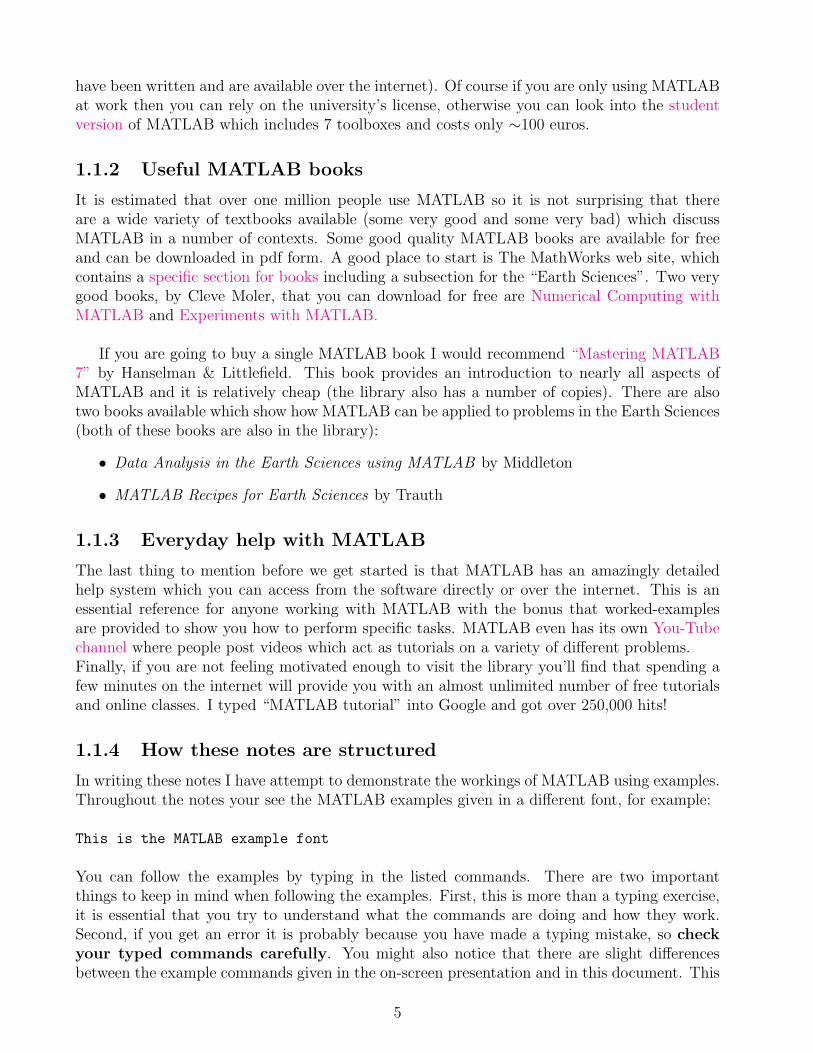
History list can also be accessed from the Command Window itself, if you place your cursor atthe >> prompt and start pressing the cursor, MATLAB will list backwards through the previouscommands. Once you have found the command you want, you can execute it by hitting theenter key.
Figure 1.2: The main MATLAB screen with the Command History highlighted in red.
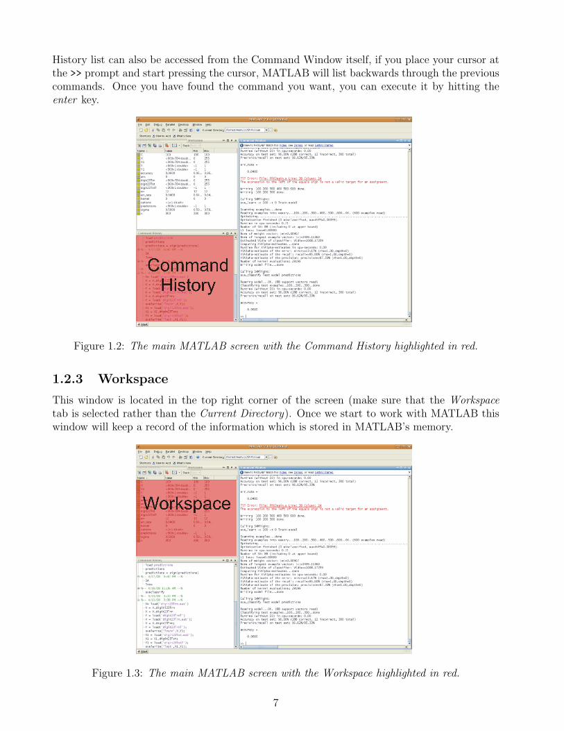
1.2.3 Workspace
This window is located in the top right corner of the screen (make sure that the Workspacetab is selected rather than the Current Directory). Once we start to work with MATLAB thiswindow will keep a record of the information which is stored in MATLAB’s memory.
Figure 1.3: The main MATLAB screen with the Workspace highlighted in red.
7

1.2.4 The Current Directory setting
Once we start loading data, we have to give MATLAB an idea where to look for the externalfiles we are interested in. If you place all you data files etc in a single location then you canchange to that directory so that MATLAB will know where to find files with specific names.
Figure 1.4: The main MATLAB screen with the Current Directory highlighted in red.
8

Chapter 2
Simple operations and working withvariables
2.1 Using variables; scalars, vectors and matrices
When you start MATLAB you will see a symbol >>. This is the prompt where commands can begiven to MATLAB. Lets start with something simple, using MATLAB like a pocket calculator.At the command prompt type:
>> 1+1
Once you press the Enter key, MATLAB will return the answer:
ans =
2
Of course we can do this with any combination of numbers and not just integers:
>> 24.7 + 2.1 + 5.6
ans =
32.4000
2.1.1 Simple scalar arithmetic
For those of you not familiar with the mathematical jargon, a scalar is simply a single number.In MATLAB a number of operations can be used to perform arithmetic with scalars.
9

Operation Symbol ExampleAddition, a + b + 3 + 22Subtraction, a - b - 90 - 54Multiplication, a × b * 3.14 * 0.85Division, a ÷ b / 56 / 8Exponentiation, ab ∧ 2 ∧ 8
2.1.2 Order of evaluation
In MATLAB there is a so-called order of evaluation for different arithmetic operators. Thismeans that the sequence in which MATLAB performs the different parts of a mathematicalexpression is fixed and we have to construct commands according to the following basic rules.
1. Parentheses (brackets), innermost first.
2. Exponentiation, left to right.
3. Multiplication and division with equal importance, left to right.
4. Addition and subtraction with equal important, left to right.
The best way to demonstrate the order of evaluation is using some basic examples. Lets takethe mean of five different numbers:
3 6 4 10 7
Of course, we need to sum the numbers and divide by 5, we could do this as two separatesteps:
>> 3 + 6 + 4 + 10 + 7
ans =
30
>> 30 / 5
ans =
6
We find the mean is 6, but from a practical point of view it is more convenient if we com-bine the steps of the calculations together. This is where the order of evaluation is importantbecause we must make sure that the total of the numbers is found before the division step. Forexample, if we ignore the order of evaluation:
>> 3 + 6 + 4 + 10 + 7 / 5
ans =
10

24.4000
In this case we get the wrong answer because the division was performed before the addi-tion (item 3. of the order of evaluation comes before point 4.). In order to do the calculationproperly we must employ parentheses:
>> (3 + 6 + 4 + 10 + 7) / 5
ans =
6
From the order of operation we can see that the expression in parenthesis (item 1.) will beevaluated before the division (item 3.), so we have the correct sequence for the calculation tobe evaluated properly.Now we’ll look at a less obvious example, which demonstrates that when two operations occurat the same point on the order of evaluation, the one on the left will be performed first.
>> 3 / 4 * 5
ans =
3.7500
>> (3 / 4) * 5
ans =
3.7500
>> 3 / (4 * 5)
ans =
0.1500
The third result is different from the first two because the parenthesis force the multiplica-tion to be evaluated before the division step even through it is on the right-hand side of theexpression.Here’s a final example which employs exponentiation, we will calculate the value of 39:
>> 3 ^ 9
ans =
19683
11

However, if we write:
>> 4 * 2 + 1
ans =
9
>> 3 ^ 4 * 2 + 1
ans =
163
We obtain the wrong answer because we have ignored the order of evaluation, to correct thisstatement we must use parenthesis to ensure that the 4 * 2 + 1 part of the expression is eval-uated before the exponentiation is performed:
>> 3 ^ (4 * 2 + 1)
ans =
19683
Exercises: order of evaluation
Given that 26.5 = 90.5097 can you added parenthesis to the following MATLAB expression toobtain a value of 90.5097.
>> 12 / 4 - 1 ^ 4 - 2 + 3 * 1.5
Next can you insert only two pairs of parentheses into the following expression to again ob-tain a value of 90.5097.
>> 4 ^ 0.5 ^ 10 - 2 ^ 1 + 1 + 0.5
2.1.3 Using named variables
Imagine you are sent to the geological hardware store to buy equipment for a fieldwork trip.On your shopping list you have the following items you wish to buy:
• 6 Geological Hammers, cost 45.32 each.
12
• 2 Compasses, cost 23.17 each.
• 9 Pocket Magnifiers, cost 4.99 each.
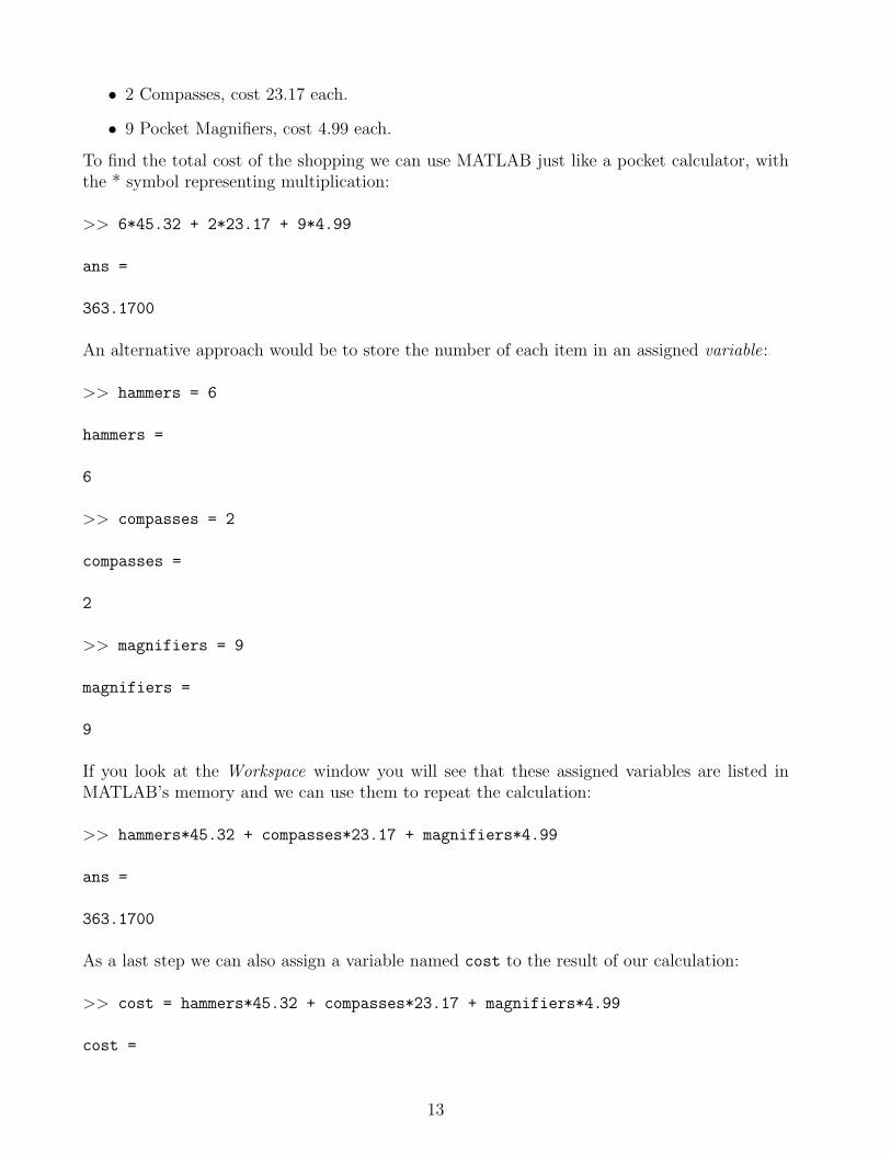
To find the total cost of the shopping we can use MATLAB just like a pocket calculator, withthe * symbol representing multiplication:
>> 6*45.32 + 2*23.17 + 9*4.99
ans =
363.1700
An alternative approach would be to store the number of each item in an assigned variable:
>> hammers = 6
hammers =
6
>> compasses = 2
compasses =
2
>> magnifiers = 9
magnifiers =
9
If you look at the Workspace window you will see that these assigned variables are listed inMATLAB’s memory and we can use them to repeat the calculation:
>> hammers*45.32 + compasses*23.17 + magnifiers*4.99
ans =
363.1700
As a last step we can also assign a variable named cost to the result of our calculation:
>> cost = hammers*45.32 + compasses*23.17 + magnifiers*4.99
cost =
13

363.1700
If we wanted to find the average cost of the items on the shopping list, we also need to knowthe total number of items, we can perform this calculation and assign the result into a variablecalled items:
>> items=hammers + compasses + magnifiers
items =
17
Remember, the variable cost is still held in MATLAB’s memory, so to find the average cost wejust perform a division using the / symbol:
>> average cost = cost / items
average cost =
21.3629
When outputting variables it is sometimes useful to use the ; symbol at the end of your expres-sion. This means MATLAB will perform the calculation and store the result in the memorybut it will not show the result on the screen. Use of the ; symbol is essential when you dealingwith large amounts of data and you don’t want to slow down your work waiting for the screento list through all the results. For example:
>> average cost = cost / items
average cost =
21.3629
Compared to:
>> average cost = cost / items; %do not show the output
MATLAB won’t accept variable names which are more than one word, therefore if we tryto use average cost rather than average−cost we receive an error:
>> average cost = cost / items
??? Undefined function or method 'average'for input arguments of type 'char'.
At anytime you can see what variables are held in the MATLAB Workspace using the whos
command:
>> whos
14
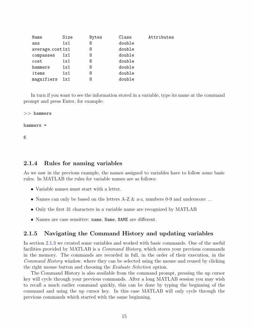
Name Size Bytes Class Attributes
ans 1x1 8 double
average cost1x1 8 double
compasses 1x1 8 double
cost 1x1 8 double
hammers 1x1 8 double
items 1x1 8 double
magnifiers 1x1 8 double
In turn if you want to see the information stored in a variable, type its name at the commandprompt and press Enter, for example:
>> hammers
hammers =
6
2.1.4 Rules for naming variables
As we saw in the previous example, the names assigned to variables have to follow some basicrules. In MATLAB the rules for variable names are as follows:
• Variable names must start with a letter.
• Names can only be based on the letters A-Z & a-z, numbers 0-9 and underscore −.
• Only the first 31 characters in a variable name are recognized by MATLAB
• Names are case sensitive: name, Name, NAME are different.
2.1.5 Navigating the Command History and updating variables
In section 2.1.3 we created some variables and worked with basic commands. One of the usefulfacilities provided by MATLAB is a Command History, which stores your previous commandsin the memory. The commands are recorded in full, in the order of their execution, in theCommand History window, where they can be selected using the mouse and reused by clickingthe right mouse button and choosing the Evaluate Selection option.
The Command History is also available from the command prompt, pressing the up cursorkey will cycle through your previous commands. After a long MATLAB session you may wishto recall a much earlier command quickly, this can be done by typing the beginning of thecommand and using the up cursor key. In this case MATLAB will only cycle through theprevious commands which started with the same beginning.
15
Lets return to the example of shopping at the geological hardware store, which we used insection 2.1.3. We have now decided that we would like to buy 7 geological hammers ratherthan 6, to update our calculations we must first change the values of the variable hammer. Wecan recall the command we used to set the variable simply by typing the first few letters andpressing the up cursor key:
>> ham Now press the up cursor
>> hammers*45.32 + compasses*23.17 + magnifiers*4.99
This is the last command to begin with ham, but it’s not the one we want so we press theup cursor again.
>> hammers = 6
This is the command we want, simply modify it to the new value and press enter.
>> hammers = 7
hammers =
7
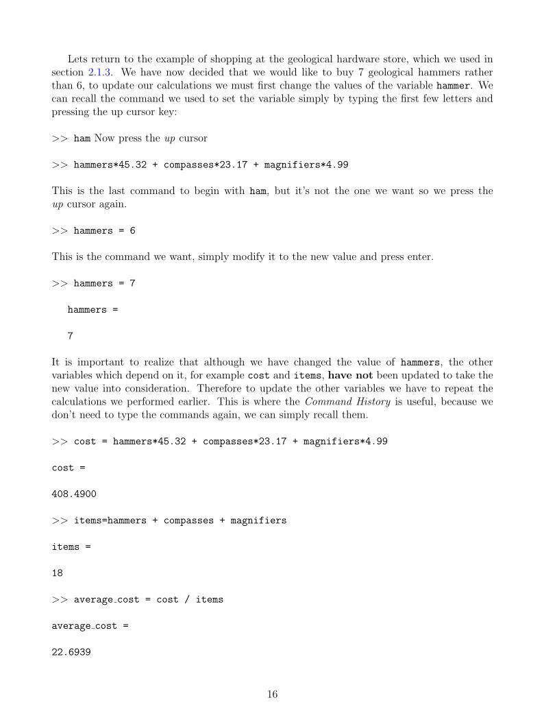
It is important to realize that although we have changed the value of hammers, the othervariables which depend on it, for example cost and items, have not been updated to take thenew value into consideration. Therefore to update the other variables we have to repeat thecalculations we performed earlier. This is where the Command History is useful, because wedon’t need to type the commands again, we can simply recall them.
>> cost = hammers*45.32 + compasses*23.17 + magnifiers*4.99
cost =
408.4900
>> items=hammers + compasses + magnifiers
items =
18
>> average cost = cost / items
average cost =
22.6939
16
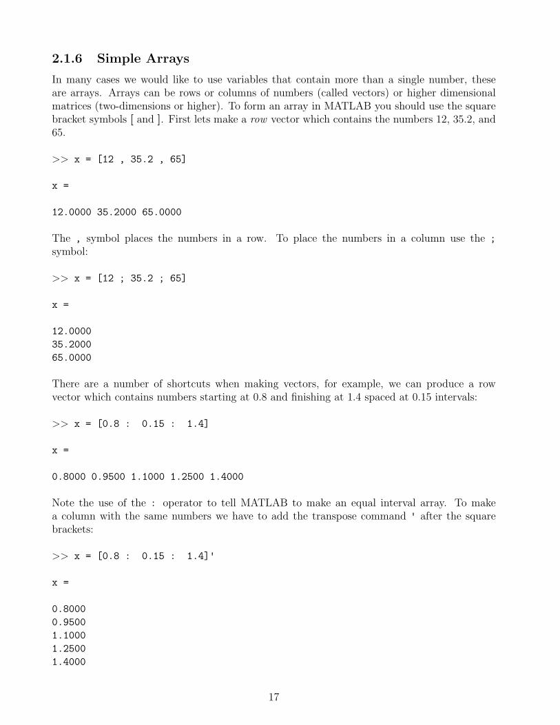
2.1.6 Simple Arrays
In many cases we would like to use variables that contain more than a single number, theseare arrays. Arrays can be rows or columns of numbers (called vectors) or higher dimensionalmatrices (two-dimensions or higher). To form an array in MATLAB you should use the squarebracket symbols [ and ]. First lets make a row vector which contains the numbers 12, 35.2, and65.
>> x = [12 , 35.2 , 65]
x =
12.0000 35.2000 65.0000
The , symbol places the numbers in a row. To place the numbers in a column use the ;
symbol:
>> x = [12 ; 35.2 ; 65]
x =
12.0000
35.2000
65.0000
There are a number of shortcuts when making vectors, for example, we can produce a rowvector which contains numbers starting at 0.8 and finishing at 1.4 spaced at 0.15 intervals:
>> x = [0.8 : 0.15 : 1.4]
x =
0.8000 0.9500 1.1000 1.2500 1.4000
Note the use of the : operator to tell MATLAB to make an equal interval array. To makea column with the same numbers we have to add the transpose command ' after the squarebrackets:
>> x = [0.8 : 0.15 : 1.4]'
x =
0.8000
0.9500
1.1000
1.2500
1.4000
17

If we have a long vector we may only be interested in certain parts of it, we can access thoseparts using an index number. Index numbers represent specific positions within an array start-ing from the first position which is given an index of 1. For example if we want to know thevalue of x at a given position:
>> x = [0.8 : 0.15 : 1.4];
>> x(3) %return the 3rd element of x
ans =
1.1000
>> x(5) %return the 5th element of x
ans =
1.4000
>> x(1:3) %the 1st through 3rd elements of x
ans =
0.8000 0.9500 1.1000
>> x([1 , 4 , 3]) %return the 1st, 4th and 3rd elements of x
ans =
0.8000 1.2500 1.1000
>> x([1 : 2 : 5]) %return the 1st, 3rd and 5th elements of x
ans =
0.8000 1.1000 1.4000
Currently the variable x holds five elements, so if we ask for the sixth we will get an errorbecause we are looking for a position which does not exist:
>> x(6) %return the 6th element of x
??? Index exceeds matrix dimensions.
You can also perform arithmetic between vectors and scalars. Construct a column vector,x, and then perform some simple calculations with it and a scalar, producing an output rowvector y:
18

>> x = [0.8 : 0.15 : 1.4]';
>> y = x + 2 %Addition of 2 to all the elements in x
y =
2.8000
2.9500
3.1000
3.2500
3.4000
>> y = x - 3 %Subtraction of 3 from all the elements in x
y =
-2.2000
-2.0500
-1.9000
-1.7500
-1.6000
>> y = x * 1.2 %Multiply all elements by 1.2
y =
0.9600
1.1400
1.3200
1.5000
1.6800
>> y = x / 2.5 %Divide all the elements by 2.5
y =
0.3200
0.3800
0.4400
0.5000
0.5600
>> y = x(1:2) + 5 %Add five to the first two elements
y =
5.8000
19

5.9500
The last type of array we will consider is the matrix which is a two or high dimensional array.The two dimensional matrix contains rows and columns. To construct a matrix we can use the, (row command) and ; (column command) operators. Note the use of the ; symbol to starta new row.
>> x = [1 , 2 , 3 , 4 ; 5 , 6 , 7 , 8]
x =
1 2 3 4
5 6 7 8
When making a matrix all the rows must have the same number of columns (as above whereeach row has 4 elements). If you try to make a matrix with rows of different lengths an errorwill be returned.
>> x = [1 , 2 , 3 , 4 ; 5 , 6 , 7 , 8 , 9]
??? Error using ==> vertcat
CAT arguments dimensions are not consistent.
A matrix has both rows and columns, so to select elements we must use both row indicesand column indices. The row index is always specified first, then the column index.
>> x = [5.4 , 7.1 , 3.3 , 2.8 ; 1.4 , 6.9 , 9.2 , 3.4]
x =
5.4000 7.1000 3.3000 2.8000
1.4000 6.9000 9.2000 3.4000
>> x(2,1) %return the element in the 2nd row and 1st column
ans =
1.4000
>> x(1,3) %return the element in the 1st row and 2nd column
ans =
3.3000
>> x(2,:) %return all the elements in the 2nd row
ans =
20

1.4000 6.9000 9.2000 3.4000
>> x(:,4) %return all the elements in the 4th column
ans =
2.8000
3.4000
2.1.7 Array-Scalar and Array-Array Arithmetic
When performing addition and subtraction on arrays you must either use an array and a scalartogether or two arrays of the same size. As a first example we will create a matrix and add ascalar to each of its entries.
>> x = [5.4 , 7.1 , 3.3 , 2.8 ; 1.4 , 6.9 , 9.2 , 3.4]
x =
5.4000 7.1000 3.3000 2.8000
1.4000 6.9000 9.2000 3.4000
>> x + 1 %add 1 to each entry in x
ans =
6.4000 8.1000 4.3000 3.8000
2.4000 7.9000 10.2000 4.4000
Addition of two arrays of the same size means they are added together element by element:
>> x + [1 , 2 , 3 , 4 ; 5 , 6 , 7 , 8]
ans =
6.4000 9.1000 6.3000 6.8000
6.4000 12.9000 16.2000 11.4000
Of course, subtraction will work in the same way. Addition or subtraction of arrays withdifferent sizes will cause an error:
>> [1 , 2 , 3 ] + [5 , 6 , 7 , 8]
??? Error using ==> plus
Matrix dimensions must agree.
21

There are two types of multiplication and division; element by element and matrix. Witharrays of the same size element by element multiplication, division and exponentiation uses the. operator. We’ll form two matrices and then perform some element by element operations.
>> x = [1 , 1 , 1 ; 2 , 2 , 2]
x =
1 1 1
2 2 2
>> y = [1 , 2 , 3 ; 4 , 5 , 6]
y =
1 2 3
4 5 6
>> x.*y %element by element multiplication
ans =
1 2 3
8 10 12
>> x./y %element by element division
ans =
1.0000 0.5000 0.3333
0.5000 0.4000 0.3333
>> x.^y %element by element exponentiation
ans =
1 1 1
16 32 64
If you don’t use the . operator MATLAB will perform matrix multiplication or division, butthe arrays must be of the correct size, for example if we try to multiply the arrays x and y:
>> x*y %matrix multiplication of x and y
??? Error using ==> mtimes
Inner matrix dimensions must agree.
22
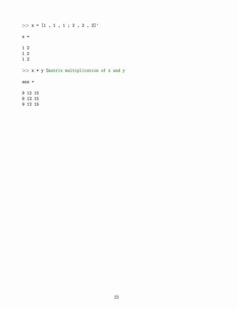
>> x = [1 , 1 , 1 ; 2 , 2 , 2]'
x =
1 2
1 2
1 2
>> x * y %matrix multiplication of x and y
ans =
9 12 15
9 12 15
9 12 15
23
Chapter 3
MATLAB Functions
3.1 Script M-files and the MATLAB Editor
As you can probably see already, when working with commands in MATLAB you will oftenwant to repeat and change specific things as you develop your code. The best way to do thisis using the built-in M-Editor to work with a sequence of commands which you can execute atany time. The commands can be stored in an M-file (with the extension *.m), so you can keepa record of your work and gradually develop the code. To create a new M-file:
1. Click on File in the main MATLAB window
2. Select New
3. Select M-file
the editor will appear with a blank document. We can now store our commands here (they mustbe kept in the correct sequence) and execute them at anytime by giving the name of the M-filein the command window, or highlighting specific commands with the mouse, giving a right-clickand choosing “evaluate selection”. I have made an example M-file with the commands we usedin the previous example, it has the name shopping.m and can be loaded from the commandwindow by typing:
>> open shopping
Using the editor provides us with a much more flexible way to issue commands to MATLAB,we can review the overall structure of a piece of code and gradually make modifications and im-provements. Within the editor we can also add comments to the M-code, these are notes whichMATLAB will ignore but provide a description of the code to remind us what is happening.Once we place a % symbol in the code, MATLAB will ignore the remainder of the line. Theeditor highlights comments in green, you can see an example of comments in the shopping.m
file.
Listing of shopping.m:
hammers = 6 %define number of hammers
24

compasses = 2 %define number of compasses
magnifiers = 9 %define number of magnifiers
%in the next line sum the total cost
cost = hammers*45.32 + compasses*23.17 + magnifiers*4.99
items = hammers + compasses + magnifiers %number of items
average cost = cost /items %calculate average cost
3.2 Working with “inbuilt” functions
The real power of MATLAB comes from its thousands of inbuilt functions. Each function isa sequence of MATLAB commands which will perform a specific task. Each function has aspecific set of input and outputs according to the information it requires and the result it willproduce. Later we will look at how we can write our own functions to perform a given task,but for the time being we will look at inbuilt functions to understand how they work.
3.2.1 Taking the square root
To find the square root of a number is simple and we could use standard MATLAB arithmeticcommands. For example to find the square root of 9:
>> 9^0.5
ans =
3
We can perform the same task on a vector as long as we use the element by element ap-proach:
>> [9 , 16 , 25].^0.5 %note the use of the dot
ans =
3 4 5
This is easy enough, but MATLAB also contains an inbuilt function called sqrt which canperform this task for us. To use a function we give its name at the command line and placethe input within brackets. The input can be a series of numbers, a variable or an expressionincluding other variables, finally the output of the function can also be assigned a specific vari-able name.
>> sqrt(9)
ans =
25

3
The sqrt function can also be used for vectors, matrices and expressions:
>> x = [9 , 16 , 25]
x =
9 16 25
>> sqrt(x)
ans =
3 4 5
>> y = sqrt(2*x+4) %assign the output to y
y =
4.6904 6.0000 7.3485
3.2.2 The help command
If you want information on what a function does and what its inputs and outputs should bethen you can used MATLAB’s help system. Simply give the help command followed by thename of the function you are interested in. This will provide detailed information on what thefunction does, other related functions which might also be useful, and a link to the function’spage in the help documentation.
>> help sqrt
SQRT(X) is the square root of the elements of X. Complex
results are produced if X is not positive.
See also sqrtm, realsqrt, hypot.
Overloaded functions or methods (ones with the same name in other directories)
help sdpvar/sqrt.m
help ncvar/sqrt.m
help sym/sqrt.m
Reference page in Help browser
26
doc sqrt
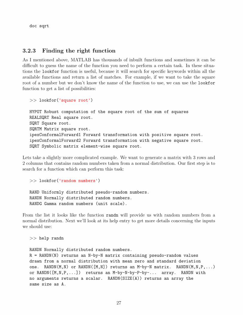
3.2.3 Finding the right function
As I mentioned above, MATLAB has thousands of inbuilt functions and sometimes it can bedifficult to guess the name of the function you need to perform a certain task. In these situa-tions the lookfor function is useful, because it will search for specific keywords within all theavailable functions and return a list of matches. For example, if we want to take the squareroot of a number but we don’t know the name of the function to use, we can use the lookfor
function to get a list of possibilities:
>> lookfor('square root')
HYPOT Robust computation of the square root of the sum of squares
REALSQRT Real square root.
SQRT Square root.
SQRTM Matrix square root.
ipexConformalForward1 Forward transformation with positive square root.
ipexConformalForward2 Forward transformation with negative square root.
SQRT Symbolic matrix element-wise square root.
Lets take a slightly more complicated example. We want to generate a matrix with 3 rows and2 columns that contains random numbers taken from a normal distribution. Our first step is tosearch for a function which can perform this task:
>> lookfor('random numbers')
RAND Uniformly distributed pseudo-random numbers.
RANDN Normally distributed random numbers.
RANDG Gamma random numbers (unit scale).
From the list it looks like the function randn will provide us with random numbers from anormal distribution. Next we’ll look at its help entry to get more details concerning the inputswe should use:
>> help randn
RANDN Normally distributed random numbers.
R = RANDN(N) returns an N-by-N matrix containing pseudo-random values
drawn from a normal distribution with mean zero and standard deviation
one. RANDN(M,N) or RANDN([M,N]) returns an M-by-N matrix. RANDN(M,N,P,...)
or RANDN([M,N,P,...]) returns an M-by-N-by-P-by-... array. RANDN with
no arguments returns a scalar. RANDN(SIZE(A)) returns an array the
same size as A.
27

This tells us the the function will return a matrix of normally distributed random numbers,the first input to the function is the number of rows for the matrix and the second is the num-ber of columns (remember we wanted 3 rows and 2 columns). We’ll name our output from thefunction z.
>> z = randn(3,2)
z =
-0.4326 1.1909
-1.6656 -1.1465
0.1253 0.2877
3.2.4 Multiple inputs and outputs
It is also possible for functions to work with multiple inputs and outputs. A good example isthe sortrows function which sorts a matrix of values from lowest to highest based on the valuesin one of its columns. The primary output of the function is the sorted matrix, but a secondaryoutput giving the index of the sorted values is also available. First we will sort the randomnumbers in z according to the values in the first column (if we don’t specify which column tobase the sort upon, MATLAB will automatically use the first).
>> y = sortrows(z) %sort the rows according to the first column
y =
-1.6656 -1.1465
-0.4326 1.1909
0.1253 0.2877
Now we’ll also use the second (optional) output of the function that records the original indicesof the sorted values (which we will call idx). Note that in order to obtain multiple outputs wehave to group them together in square brackets when calling the function:
>> [y,idx] = sortrows(z) %sort the rows by the first column and return the indices
y =
-1.6656 -1.1465
-0.4326 1.1909
0.1253 0.2877
idx =
28
2
1
3
Finally, we’ll supply the function with a second (optional input argument) which gives the indexof the column upon which the sort should be based. In this case we will sort according to thevalues in the second column:
>> [y,idx] = sortrows(z,2)
y =
-1.6656 -1.1465
0.1253 0.2877
-0.4326 1.1909
idx =
2
3
1
3.3 Exercise: Mmmm, π
Now it’s your turn. Throughout the class we will attempt to solve problems using MATLABby applying the topics which have been discussed. Some of you may find them relatively easily(especially if you have some experience of MATLAB) and others will find them more difficult. Ihave specifically designed the exercises to be challenging, so don’t expect to finish them withina few minutes. It is important to realize that MATLAB is a tool and will only help you to solvea problem if you know how the problem should be solved. The first question you should askyourself is “what method will I used to solve the problem?” and only then should you thinkabout “how can I implement my method in MATLAB?”. For this first exercise we are going tolook at a simple numerical problem involving π.
Approximating π
The value of π has a very simple definition, “the ratio of a circle’s circumference to its diameter”,but it is irrational number, meaning its decimal representation never ends or repeats.
29

Figure 3.1: The π pie. If the pie is a perfect circle then the ratio of its circumference (red line)to its diameter (blue line) is equal to π
.
Determining a more and more accurate evaluation of π is still an active area of research,current estimates have a precision of over 100000000000 decimal places (at the beginning of2010 Fabrice Bellard announced that he had calculated π to 2.7 trillion digits). To give you aflavor of what some people’s research involves, the first 1000 digits of π are:
3.14159265358979323846264338327950288419716939937510582097494459230781640628620899862803482534211706798214808651328230664709384460955058223172535940812848111745028410270193852110555964462294895493038196442881097566593344612847564823378678316527120190914564856692346034861045432664821339360726024914127372458700660631558817488152092096282925409171536436789259036001133053054882046652138414695194151160943305727036575959195309218611738193261179310511854807446237996274956735188575272489122793818301194912983367336244065664308602139494639522473719070217986094370277053921717629317675238467481846766940513200056812714526356082778577134275778960917363717872146844090122495343014654958537105079227968925892354201995611212902196086403441815981362977477130996051870721134999999837297804995105973173281609631859502445945534690830264252230825334468503526193118817101000313783875288658753320838142061717 76691473035982534904287554687311595628638823537875937519577818577805321712268066130019278766111959092164201989
Over time people have used a number of different approximations for π, a popular one is 227
.Probably the strangest is a legal bill which was proposed in 1897 that would set pi = 3.2 inorder that people could remember it more easily. There is a long history of methods with whichto approximate π, one of the most elegant of which was given in the 14th century by the Indianmathematician Madhava of Sangamagrama (interestingly the technique was “rediscovered” inEurope over 300 years later). Madhava of Sangamagrama showed that π
4could be obtained as
the sum of an infinite series:
∞∑n=0
(−1)n
2n+ 1=π
4
Therefore if we work with the first 4 terms, for n=0 to n=3 and ultimately working to infinitywe would get:
30

(−1)0
2 ∗ 0 + 1+
(−1)1
2 ∗ 1 + 1+
(−1)2
2 ∗ 2 + 1+
(−1)3
2 ∗ 3 + 1+ . . .
(−1)∞
2 ∗∞+ 1=π
4
the beginning of which simplifies to:
1− 1
3+
1
5− 1
7+ . . . =
π
4
We’re going to use this approach to estimate π in MATLAB. Obviously we can’t calculate aninfinite number of terms so we’ll only work to a maximum of n = 10000. One function youmight find useful is sum, look at its help entry to get more information about its use. For thoseof you familiar with MATLAB this exercise won’t be too much of a challenge so you should tryto perform same task whilst playing MATLAB “golf”. That is, what is the smallest number ofcharacters you can use in your code to make the calculation (mine was 30 characters). I wouldrecommend that you work in the editor in order that you can develop and modify your codemore easily.
Steps to completing the exercise
There are three main tasks to solve this exercise:
1. Generating the numbers between 0 and 10000 to act as n.
2. Calculating the terms of the series using the values of n.
3. Finally, summing the series and multiplying by 4 to estimate π.
Functions you may find useful
• sum - Sum of array elements.
3.4 Writing your own functions
One of the great advantages of MATLAB is the capacity to write your own functions withspecific inputs and outputs. This means you can design and write your own processing routineswhich can be used over and over again with no additional effort (always a good thing!).
3.4.1 Inline functions
If you have a simple expression with a single output you can define it as an inline function sothat it can be used repeatedly without retyping the code. For example, imagine we want tostudy the equation for a variety of values f and θ:
31
g = sin(2 ∗ π ∗ f + θ)
We can use the inline function to define this expression and its input, so that it can be calledrepeatedly. Note that during the definition of the inline function the expression and input vari-able names are defined as character strings.
>> g = inline('sin(2*pi*f + theta)', 'f', 'theta')
g =
Inline function:
g(f,theta) = sin(2*pi*f + theta)
>> g(0.5,pi./4)
ans =
-0.707106781186547
Inline functions are useful for simple expressions, but in more complex situations it is necessaryto create an M-function.
3.4.2 M-functions
It is simple to write your own M-functions with specific input and outputs. An M-function isa separate M file (normally written in the MATLAB editor), which is a sequence of MATLABcommands, working with provided inputs and producing a specific output. The key to anM-function is the first line of the function, which defines 4 things in order:
1. That the file contains a function
2. The output variables of the function
3. The name of the function
4. The input variables of the function
We’ll start with a example of a function called simple, which has one input x and one outputy. The operation of the function takes the value of x, adds one to it and outputs the result asy. Start a new M-file in the editor and enter the following text.
function y=simple(x)
y=x+1;
32

When you try to save the function, MATLAB will suggest the same name as you defined for thefunction (simple.m). When searching for a function MATLAB actually refers to the filenamerather than the defined name inside the function, so it’s essential that they match each other.Now we can call the function simple in the same way as any other MATLAB function. Forexample:
>> x = 5
>> y = simple(x)
y =
6
The the names of the input, x, and output, y, are only used within the function, so whenwe are calling the function externally (i.e. from outside) we can use any names we want. Forexample:>> a = 5
>> b = simple(a)
b =
6
One of the advantages of M-functions is that all the variables which may be created by theintermediate steps of the function will not be stored in the MATLAB memory once the calcula-tion is complete, only the output is stored. This makes functions a very tidy way of performingcertain tasks because only the output is stored. We can set multiple inputs and outputs sim-ply by adding them to the first line of the function. The next function we’ll write is calledsimple2.m, which takes two inputs c and d and gives two outputs, e which is the difference of cand d, and f which is the sum of c and d. Note that comments can also be included to explainthe steps of the function.
function [e,f]=simple2(c,d)
e = c - d; %find the difference
f = c + d; %find the sum
Now we must supply two input names and two output names. For example:
>> cats=7;
>> dogs=4;
>> [shirt,socks]=simple2(cats,dogs)
shirt =
3
33
socks =
11
Hopefully this will convince you that you can use any variable names, of course it is always bestto use meaningful names which describe the variable.
Including help and comments
One key aspect of writing functions is including detailed help so that other people can use yourfunction and comments which show how the calculations are performed. Often you will writea function and after not looking at it for a few months you will have forgot how it works orhow to use it. In these situations the help information and comments are invaluable. Help isentered after the first line of the file and is basically a series of comments, however, because oftheir position MATLAB can find them whenever you use the help or lookfor functions.We take an example from probably the worlds most famous equation, the mass-equivalencerelationship:
E = mc2
where E is energy, m is mass and c is the speed of light. We can write a vanilla function (i.e.the most simple form) without help or comments.
function E=massequiv0(m)
c = 299792458;
E = m*c^2;
In this form the function will work and return the correct answer. It is obvious what is hap-pening because we are only performing a simple operation. However some functions requirethousands of lines of code, thus it is very easy to become lost and the meanings of differentvariable names maybe obscure. Therefore it is always a good idea to include some commentsthat describe what is happening in the different lines of code. For an equation such as this it isalso a good idea to state which units are being used.
function E=massequiv1(m)
c = 299792458; %speed of light [m s^-1]
E = m.*c.^2; %calculate the energy in Joules [kg m^2 s^-2]
Things are starting to improve, but we still have to include the help information. The help isessential because it describes what the function does and what the different inputs and outputsrepresent.
34
function E=massequiv2(m)
%massequiv2 - Find energy from mass based on Einstein (1905)
%
% Syntax: energy = massequiv2(mass)
%
% Inputs:
% m - mass [kg]
%
% Outputs:
% E - equivalent energy [Joules or kg m^2 s^-2]
%
% Other m-files required: none
% Subfunctions: none
% MAT-files required: none
%
% Author: Dave Heslop
% Department of Geosciences, University of Bremen
% email address: [email protected]
% Last revision: 6-Dec-2008
%------------- BEGIN CODE --------------
c = 299792458; %speed of light [m s^-1]
E = m.*c.^2; %calculate the energy in Joules [kg m^2 s^-2]
%------------- END CODE --------------
With the help information in place we can use the lookfor and help functions:>> lookfor Einstein
>> help massequiv2
35

3.5 Exercise: Mmmm, a second helping of π
In this exercise simply convert the script file you created for the evaluation of π into a M-function.The input for the function should be N, the number of terms to include in the evaluation andthe output p is the final evaluation of π. Don’t forget to include help and comments.
Steps to completing the exercise
There are three main tasks to solve this exercise:
1. Add a header line defining the function name (madhava), the input (N) andoutput (p).
2. Define the values of n to be used as ranging between 0 and N
3. Add suitable help and comments (see previous examples)
Functions you may find useful
• sum - Sum of array elements.
36
3.6 Exercise: The Geiger counter
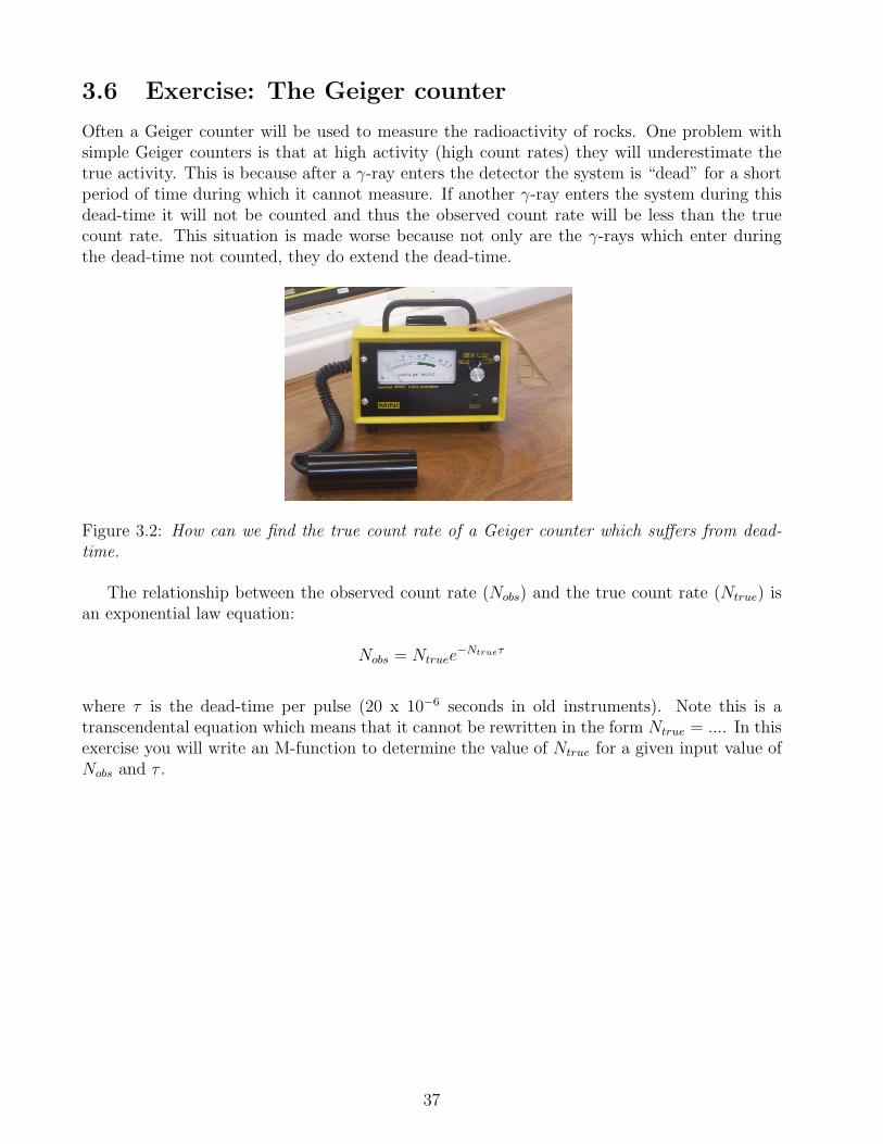
Often a Geiger counter will be used to measure the radioactivity of rocks. One problem withsimple Geiger counters is that at high activity (high count rates) they will underestimate thetrue activity. This is because after a γ-ray enters the detector the system is “dead” for a shortperiod of time during which it cannot measure. If another γ-ray enters the system during thisdead-time it will not be counted and thus the observed count rate will be less than the truecount rate. This situation is made worse because not only are the γ-rays which enter duringthe dead-time not counted, they do extend the dead-time.
Figure 3.2: How can we find the true count rate of a Geiger counter which suffers from dead-time.
The relationship between the observed count rate (Nobs) and the true count rate (Ntrue) isan exponential law equation:
Nobs = Ntruee−Ntrueτ
where τ is the dead-time per pulse (20 x 10−6 seconds in old instruments). Note this is atranscendental equation which means that it cannot be rewritten in the form Ntrue = .... In thisexercise you will write an M-function to determine the value of Ntrue for a given input value ofNobs and τ .
37

Steps to completing the exercise
When writing your M-function you will need to think about the inputs and outputsthe function will require. The required inputs should follow the basic lines of:
• The observed count rate (called Nobs)
• The dead-time (called tau)
• The array of integer count rate values to test (called Ntest)
For the calculation itself we need to determine the calculated count rate Ncalc for eachof the guesses in Ntest and then find which one fits best with the observed count rate,Nobs. This will involve the following steps:
1. Determine the values of Ncalc which would be measured for your values of Ntrue.
2. Determine which value of Ncalc is closest to the value of Nobs measured on theGeiger counter.
3. Output the value of Ntest corresponding to the best prediction of Nobs.
Functions you may find useful
• exp - Exponential
• sort - Sort array elements in ascending or descending order.
• sqrt - Square root
38
Chapter 4
Relational and logical operators
4.1 Relational and logical operations
The purpose of relational and logical operators is to provide answers to True/False questions.To represent this idea numerically MATLAB uses a system based on:
• True = 1
• False = 0
4.1.1 Relational testing
As an example, relational operators can be used to test if two numbers are equal, or if onenumber is greater than another. MATLAB uses the following relational operators:
Relational Operator Description< less than<= less than or equal to> greater than>= greater than or equal to== equal to∼= not equal to
These operators can be used to compare both scalars and arrays. For example, working withscalars:
>> A = 5;
>> B = 6;
>> A == B %test if A is equal to B
ans =
0
39

>> A ∼= B %test if A does not equal B
ans =
1
>> A >= B %test if A is greater than or equal to B
ans =
0
>> A < B %test if A is less than B
ans =
1
When we work with arrays the relationships are tested on a element-by-element basis. Theoutput will be the same size as the array being tested, with the position of ones and zeros inthe output corresponding to the elements being tested:
>> A = [1:1:5]
A =
1 2 3 4 5
>> B = [5:-1:1]
B =
5 4 3 2 1
>> A >= 4 %positions where A is greater-than or equal to 4
ans =
0 0 0 1 1
>> A == B %positions where A equals B
ans =
0 0 1 0 0
>> B < A %positions where B is less-than A
40
ans =
0 0 0 1 1
In the case where the two arrays are not the same size, MATLAB will return an error be-cause it is not possible to perform an element-by-element comparison:
>> A = [1:1:4]
A =
1 2 3 4
>> B = [1:1:3]
B =
1 2 3
>> A == B
??? Error using ==> eq
Matrix dimensions must agree.
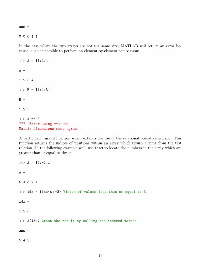
A particularly useful function which extends the use of the relational operators is find. Thisfunction returns the indices of positions within an array which return a True from the testrelation. In the following example we’ll use find to locate the numbers in the array which aregreater than or equal to three:
>> A = [5:-1:1]
A =
5 4 3 2 1
>> idx = find(A>=3) %index of values less than or equal to 3
idx =
1 2 3
>> A(idx) %test the result by calling the indexed values
ans =
5 4 3
41

4.1.2 Logical Operators
Logical operators allow us to combine a series of relational expressions. In this way we canspecify in detail a series of relations which a given number must meet or not meet.
Logical Operator Description& AND| OR∼ NOT
As a first example we’ll compare to vectors A and B to find where A is greater than B, with theadded condition that the only results which are acceptable are those where A does not equal 5.
>> A = [1:1:5]
A =
1 2 3 4 5
>> B = [5:-1:1]
B =
5 4 3 2 1
>> A > B & A∼=5 %find A is greater than B and A does not equal 5
ans =
0 0 0 1 0
We can see from this result that the fifth element of A meets the first requirement (>B), but notthe second (∼=5), so a result of False is returned. Only the fourth element of meets both re-quirements. The logical operators can also be included when using the find function. We’ll workwith the same variable B, and find the values which are less than or equal to 2 or greater than 4.
>> idx = find(B<=2 | B>4)
idx =
1 4 5
>> B(idx) %check the result
ans =
42
5 2 1
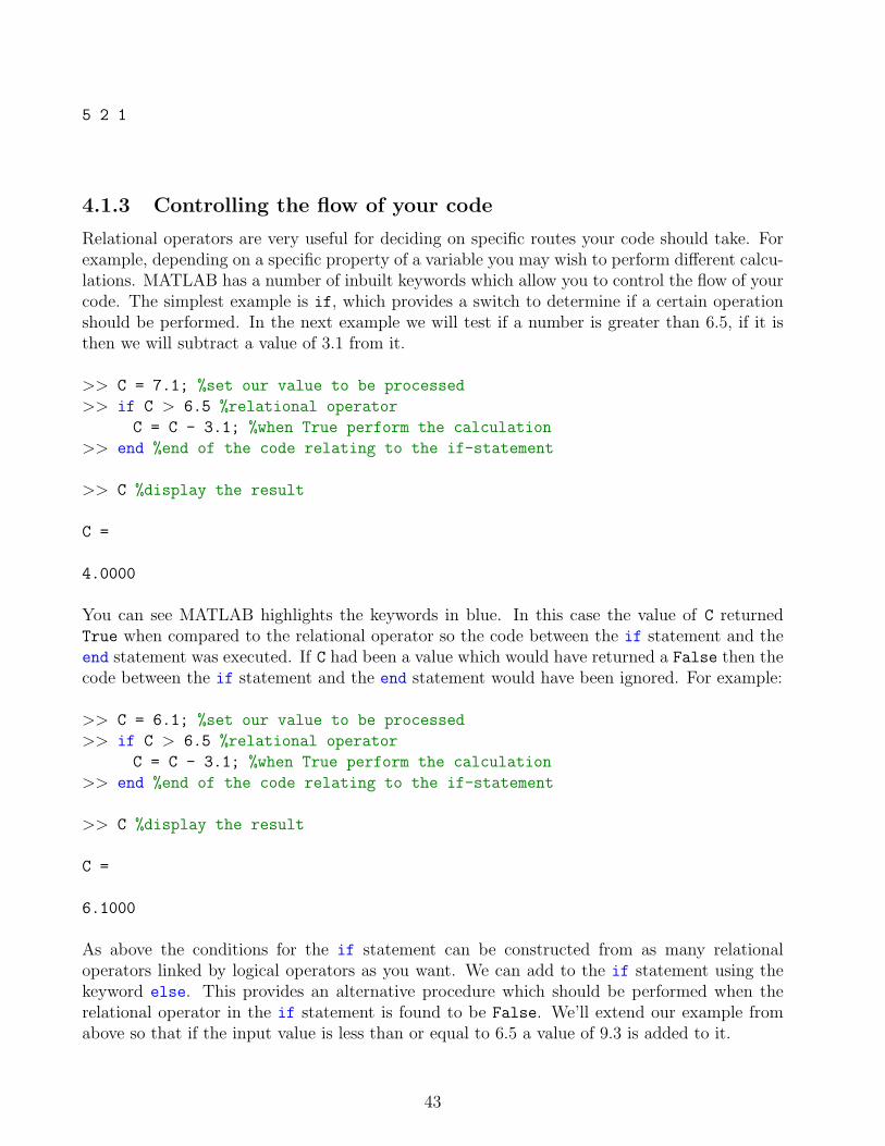
4.1.3 Controlling the flow of your code
Relational operators are very useful for deciding on specific routes your code should take. Forexample, depending on a specific property of a variable you may wish to perform different calcu-lations. MATLAB has a number of inbuilt keywords which allow you to control the flow of yourcode. The simplest example is if, which provides a switch to determine if a certain operationshould be performed. In the next example we will test if a number is greater than 6.5, if it isthen we will subtract a value of 3.1 from it.
>> C = 7.1; %set our value to be processed
>> if C > 6.5 %relational operator
C = C - 3.1; %when True perform the calculation
>> end %end of the code relating to the if-statement
>> C %display the result
C =
4.0000
You can see MATLAB highlights the keywords in blue. In this case the value of C returnedTrue when compared to the relational operator so the code between the if statement and theend statement was executed. If C had been a value which would have returned a False then thecode between the if statement and the end statement would have been ignored. For example:
>> C = 6.1; %set our value to be processed
>> if C > 6.5 %relational operator
C = C - 3.1; %when True perform the calculation
>> end %end of the code relating to the if-statement
>> C %display the result
C =
6.1000
As above the conditions for the if statement can be constructed from as many relationaloperators linked by logical operators as you want. We can add to the if statement using thekeyword else. This provides an alternative procedure which should be performed when therelational operator in the if statement is found to be False. We’ll extend our example fromabove so that if the input value is less than or equal to 6.5 a value of 9.3 is added to it.
43

>> C = 6.1; %set our value to be processed
>> if C > 6.5 %relational operator
C = C - 3.1; %when True perform the calculation
else %enter the alternative for a False
C = C + 9.3;
>> end
>> C %display the result
C =
15.4000
Our value of 6.1 returned False when tested against the relational operator at the if statement,so the code corresponding to the else statement was executed. We can even make these alter-native pieces of code conditional using the elseif statement and a further relational operator.We’ll modify the above example in order that 9.3 is only added to the value if the startingnumber is less than 2.4.
>> C = 6.1; %set our value to be processed
>> if C > 6.5 %relational operator
C = C - 3.1; %when if is True perform the calculation
>> elseif C < 2.4 %enter the alternative condition
C = C + 9.3; %when elseif is True perform the calculation
>> end
>> C %display the result
C =
6.1000
4.1.4 For Loops
There are a number of other ways of controlling the flow of your code, for example the for
command which is very useful when we want to repeat the same operation a specific numberof times. For loops are commonly used in other programming languages such as FORTRANto repeat specific tasks, they are also possible in MATLAB but computationally expensive, sothey should be avoided when possible. For loops depend on a variable which is set as a counterthat will run for a specific number of cycles. For example, we’ll use a counter i which will loopbetween the value of 1 and 5, for each cycle of the loop we will print the value of i on the screen.
>> for i=1:5
i %print the value of i on the screen
>> end
i =
44
1
i =
2
i =
3
i =
4
i =
5
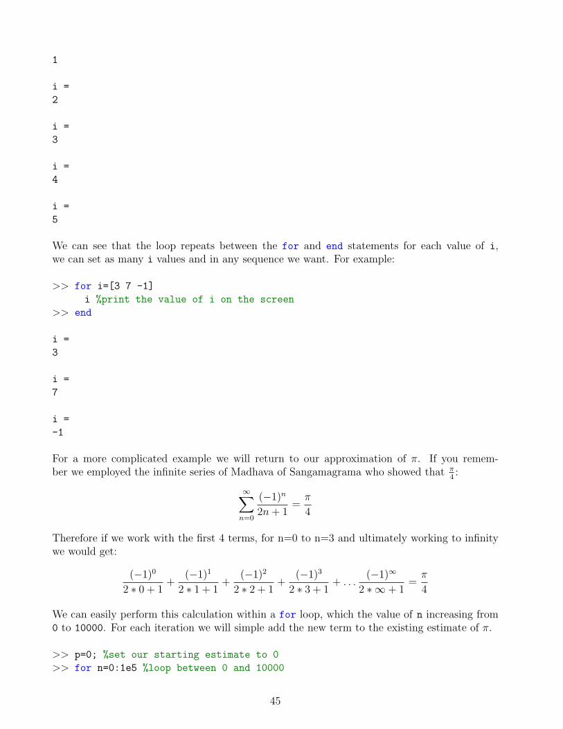
We can see that the loop repeats between the for and end statements for each value of i,we can set as many i values and in any sequence we want. For example:
>> for i=[3 7 -1]
i %print the value of i on the screen
>> end
i =
3
i =
7
i =
-1
For a more complicated example we will return to our approximation of π. If you remem-ber we employed the infinite series of Madhava of Sangamagrama who showed that π
4:
∞∑n=0
(−1)n
2n+ 1=π
4
Therefore if we work with the first 4 terms, for n=0 to n=3 and ultimately working to infinitywe would get:
(−1)0
2 ∗ 0 + 1+
(−1)1
2 ∗ 1 + 1+
(−1)2
2 ∗ 2 + 1+
(−1)3
2 ∗ 3 + 1+ . . .
(−1)∞
2 ∗∞+ 1=π
4
We can easily perform this calculation within a for loop, which the value of n increasing from0 to 10000. For each iteration we will simple add the new term to the existing estimate of π.
>> p=0; %set our starting estimate to 0
>> for n=0:1e5 %loop between 0 and 10000
45

pnew=((-1).^n./(2*n+1))*4; %find the newest term
p=p+pnew; %add the new term to the estimate
>> end %end the loop
>> p =
3.1416
One particularly useful feature of loops is that you can use the counter variable as an in-dex to place data into an output variable. In this next example we want store each term of theseries into an output array.
>> pterm=zeros(1e5,1); %setup an output array with zeros
>> for n=0:1e5 %loop between 0 and 10000
pterm(n+1)=((-1).^n./(2*n+1))*4; %note the index is n+1
>> end %end the loop
>> pterm %view the output on the screen
We now have each term stored in sequence in variable pterm. Note that because the indexof the first position in a MATLAB array is 1, but out first value of n is 0, we always have touse an index of n+1.
4.2 Exercise 1: Classifying sediments
Often sediments are grouped according to their grain size. In this example we’ll look at thegrain size fractions corresponding to:
• Sand, particles with sizes greater than 1/16 µm and less than 2 µm
• Silt, particles with sizes greater than 1/256 µm and less than 1/16 µm
• Clay, particles with sizes less than 1/256 µm
Data for 100 samples is stored in the file grainsize.mat, which contains a 100 x 3 matrix ofdata called gs. The numbers in the matrix correspond to the percentage of sand (first column),silt (second column) and clay (third column), where each sample is represented by one row(therefore each row of the matrix adds to 100%). Use the relational and logical operators wediscussed above to answer the following questions.
1. How many samples contain more than 50% sand?
2. How many samples contain more than 50% silt?
3. How many samples contain more than 30% silt or more than 25% clay?
4. How many samples contain more than 40% sand, less than 40% silt and more than 40%clay?
46

Steps to completing the exercise
This exercise is pretty simple but is relies on two things:
• Correctly selecting the column of the data matrix which corresponds to the grainsize fraction you are interested in.
• Constructing relational and logical operators to test which samples fulfill thegiven criteria.
To determine the number of samples which fulfill the a criteria you can either:
1. Find the sum of the array returned by the logical operator (i.e. add up the 1sand 0s).
2. Use the find function to return the index positions of the samples which meetthe criteria and then determine the total number of returned positions.
Functions you may find useful
• sum - Sum of array elements.
• numel - Number of elements in array.
4.3 Exercise 2: The Safe Cracker
We’re going to write a function that simulates trying to find the code which will open a safe fullof money. The safe has a three-digit combination which must be entered into the function andthe output must say wether the safe stays locked or opens (you can represent this numerically,for example a returned 0 represents “locked”, a 1 represents “open”).
47

Figure 4.1: The safe requires the correct 3 digit combination to be opened.
Our safe, however, has a slight design problem which will help us to find the combination.The safe will tell us which digits are wrong and which are correct, for example:
The first digit is incorrect.
The second digit is correct.
The third digit is incorrect.
You can send text messages to the MATLAB command window using the function disp. Writean M-file using logical operators which will simulate this safe.
48

Steps to completing the exercise
This exercise as a whole has a number of things you must consider beyond simply howto test if a series of numbers are the same or not:
• Handling input (the guess of the combination) and output (indicator if the safeopens or not).
• Testing the guessed combination against the true combination.
• Determining if the safe should open or not.
You can approach these different parts using the various topics we have studied in thepast chapters:
1. Input and output can be handled by constructing an M-function.
2. Testing if the digits of the guessed combination and true combination are thesame can be performed using relational operators.
Functions you may find useful
• disp - Display text or array.
As a simple example here is a script with which we can test if two numbers A and Bare the same and output the result to the screen. You should be able to adapt thisexample for your own solution:
A=5
B=6
if A==B
disp(’The numbers are the same’)
else
disp(’The numbers are different’)
end
4.3.1 An even worse safe
Once you have written your function, modify it so that the guess does not need to be so accuratefor the lock to open. Construct the function so that a guessed digit only has to be within ±1
49
of the true number in order for it to be accepted as correct.
Steps to completing the exercise
This exercise only requires some simple modifications to your previous M-function. Itmight be a good idea to save your modified function with a new name so you don’toverwrite your previous work. For the previous exercise you tested if the guessed digitswere equal to the true combination, now you need to check if the guess digit is within±1 of the true combination. In other words you must test if a digit is greater than orequal to the the true digit minus 1 and less than or equal to the true digit plus 1, soyou’ll need to use a logical operator to test both cases simultaneously.
50
Chapter 5
Input / Output and data management
How can we import and export data from the MATLAB workspace? This can be a surprisinglycomplicated question to answer and depending on what kind of data you are working with youmay want to consider a number of different approaches. Of course the advantage of MATLABis that once you have found the best way to import your data you can write a function whichwill perform the task automatically.
5.1 Import
We’ll look at the following ways in which you can import your data into MATLAB.
• Copy and Paste.
• Loading from an ASCII text file.
• Low-level I/O functions.
• Import from an EXCEL workbook.
• Reading from a NetCDF file.
Each of these methods has both advantages and disadvantages, so often it is best to give a littlethought as to which technique will work best for your data. One important thing to rememberis that MATLAB cannot mix text and numbers, so you can’t have column headers as you wouldhave in EXCEL.
5.1.1 Copy and Paste
This is probably the simplest import method but it is also the most cumbersome. We’ll use thefunction clipboard (which requires the Sun Microsystems Java software) to paste copied datainto MATLAB. Open the file I0 example1.txt in a text editor such as Notepad or Wordpad,select the data and copy it.
51

Figure 5.1: The example data in text file IO example1.txt.
We can now paste the data from the clipboard with the command:
>> data = clipboard('pastespecial')
The import wizard will appear that allows you to check that your data looks okay. If you aresatisfied then click Next> and then Finish.
Figure 5.2: MATLAB’s import wizard allows us to review the copied data
This has created a structural array (an advanced type of data array which we won’t bediscussing in detail) called data. To convert data into a standard array we give the command:
>> data = data.A pastespecial;
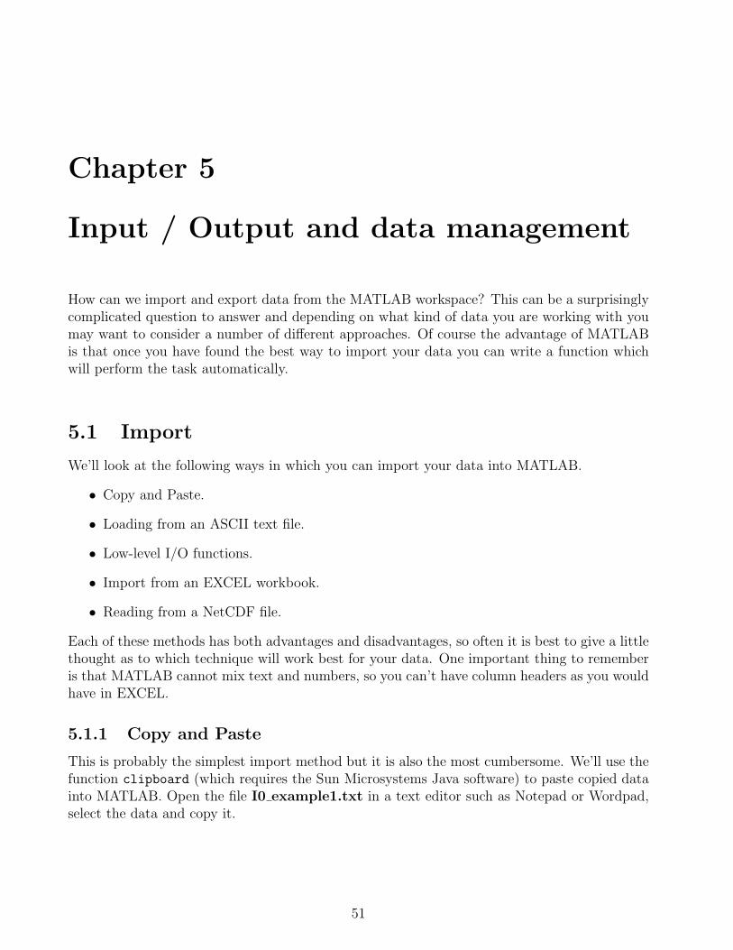
We can use the same procedure for matrices, select all the data in the file I0 example2.txtand repeat the import procedure. MATLAB can only import blocks of data which meet therequirements of scalars, vectors or matrices. In the file I0 example3.txt we can see that notall of the rows contain the same number of values (this could be a common situation whendealing with experimental data).
52
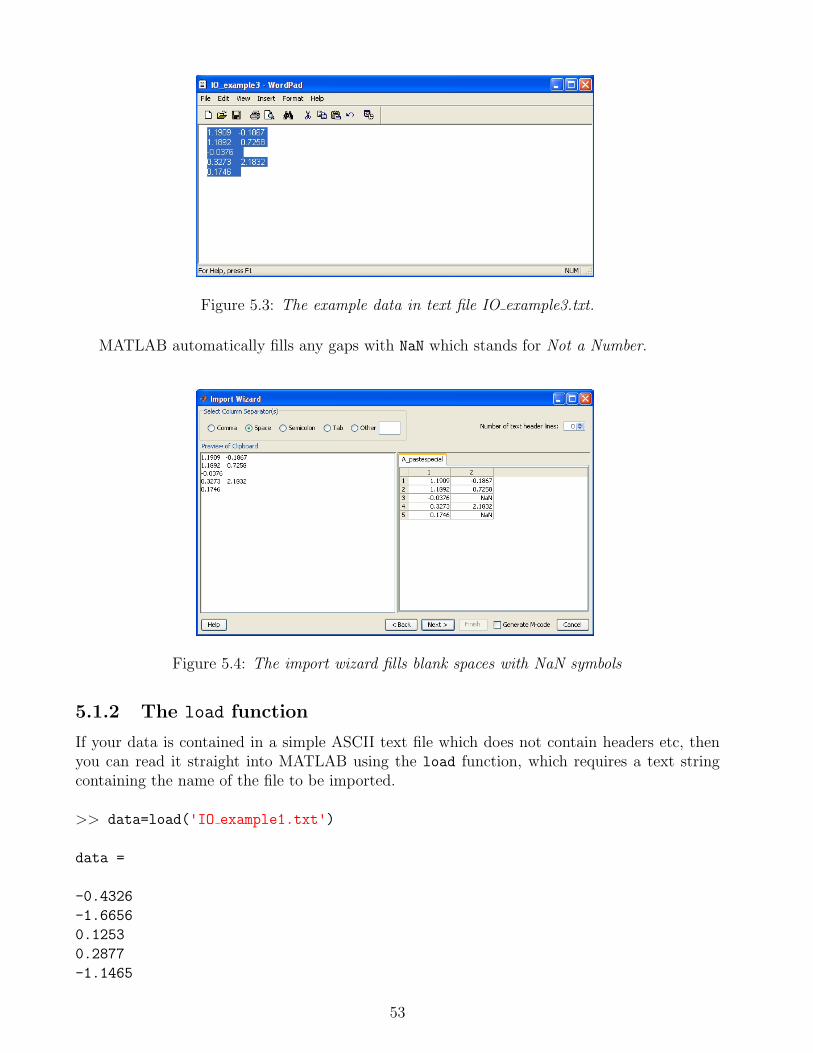
Figure 5.3: The example data in text file IO example3.txt.
MATLAB automatically fills any gaps with NaN which stands for Not a Number.
Figure 5.4: The import wizard fills blank spaces with NaN symbols
5.1.2 The load function
If your data is contained in a simple ASCII text file which does not contain headers etc, thenyou can read it straight into MATLAB using the load function, which requires a text stringcontaining the name of the file to be imported.
>> data=load('IO example1.txt')
data =
-0.4326
-1.6656
0.1253
0.2877
-1.1465
53

Unfortunately the load function cannot handle missing data values, so when we try to loadI0 example3.txt which contained gaps in the second column, MATLAB will return an error.
>> data=load('IO example3.txt')
??? Error using ==> load
Number of columns on line 2 of ASCII file F:\GLOMAR MATLAB2009\IO\IO example3.txt
must be the same as previous lines.
We also have a problem with header lines, for example, the file I0 example4.txt contains sometext:
Figure 5.5: An example data file with a text header.
MATLAB cannot combine text and numbers into one array so it returns an error when wetry to load the file:
>> data=load('IO example4.txt')
??? Error using ==> load
Unknown text on line number 1 of ASCII file F:\GLOMAR MATLAB2009\IO\IO example4.txt
"Header".
This means you have to be careful when preparing input files to make sure that they are in aform which MATLAB can understand. There are extensions to the load function which allowyou to skip header lines. The function textread allows a number of optional input argumentswhich allow you to ignore problematic objects like header lines. As a very basic example we’llprovide textread with a filename, tell it to read 64bit floating point numbers ('%n') and ignoreone header line at the top of the file:
>> data=textread('IO example4.txt','%n','headerlines',1)
data =
-0.4326
-1.6656
0.1253
54

0.2877
-1.1465
There are a number of different options for textread which allow you, for example, to de-fine delimiting characters and replacements for any missing values. Check the MATLAB helpfor more details on textread and the more advanced function textscan.
5.1.3 Low-level I/O functions
Often you will have complex data files which cannot be handled with the simple load ortextread functions. For such situations MATLAB has a collection of inbuilt functions whichassist you with the various input / output tasks. The functions are very useful if you are writ-ing your own code to import specific types of data files. Here we will only look at a very basicexample, but the functions can be combined together and used to make very complex inputroutines. In the following example we will open a text file, ignore a header line and read datainto MATLAB line by line.
>> fname='IO example4.txt' %define the file to be opened
>> fid=fopen(fname) %open the file and assign it an identification number
fid =
3
>> fgetl(fid) %read one line from the file (the header)
ans =
Header
>> input=fgetl(fid) %read the next line from the file
input =
-0.4326
>> x(1)=str2num(input) %convert the string into a number and store in x
x =
-0.4326
>> input=fgetl(fid) %read the next line from the file
input =
-1.6656
>> x(2)=str2num(input) %convert the string into a number and store in x
x =
55
-0.4326 -1.6656
>> fclose(fid) %close the file
Using these low level I/O functions provides the most flexible method to import and exportdata in MATLAB, but you will need some experience to be able to use the efficiently. You canlook on the MathWorks File-exchange for examples of how to use the functions and there arealso a number of freely-available functions which can help with import and export.
5.1.4 Import from an EXCEL workbook
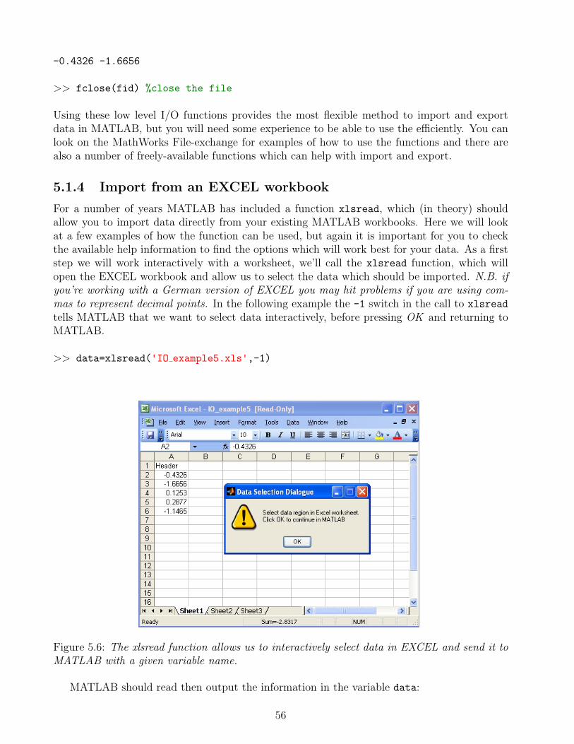
For a number of years MATLAB has included a function xlsread, which (in theory) shouldallow you to import data directly from your existing MATLAB workbooks. Here we will lookat a few examples of how the function can be used, but again it is important for you to checkthe available help information to find the options which will work best for your data. As a firststep we will work interactively with a worksheet, we’ll call the xlsread function, which willopen the EXCEL workbook and allow us to select the data which should be imported. N.B. ifyou’re working with a German version of EXCEL you may hit problems if you are using com-mas to represent decimal points. In the following example the -1 switch in the call to xlsread
tells MATLAB that we want to select data interactively, before pressing OK and returning toMATLAB.
>> data=xlsread('IO example5.xls',-1)
Figure 5.6: The xlsread function allows us to interactively select data in EXCEL and send it toMATLAB with a given variable name.
MATLAB should read then output the information in the variable data:
56
data =
-0.4326
-1.6656
0.1253
0.2877
-1.1465
It is also possible to extract data automatically from an EXCEL sheet, this requires the desiredcell position to be entered into the xlsread function. In this example we’ll use the same EXCELworkbook, extracting data from cells A2 to B6 in the worksheet “Sheet2”.
>> data=xlsread('IO example5.xls','Sheet2','A2:B6 ')
data =
0.1139 0.2944
1.0668 -1.3362
0.0593 0.7143
-0.0956 1.6236
-0.8323 -0.6918
Again, this only demonstrates the most basic functionality of xlsread. When importing yourown data read the documentation carefully.
5.1.5 NetCDF files
For those of you who work with large data sets, for example output from climate models orsatellite observations, you will probably want to load data from NetCDF files into MATLAB.Importing from NetCDF into MATLAB is not built into MATLAB but a number of differentfunctions have been written by the scientific community and are available for free downloadfrom various web sites. In my experience the best package is the NetCDF Toolbox which isavailable from http://mexcdf.sourceforge.net/. This package will provide you with routinesfor reading, modifying and creating NetCDF files.
5.2 Export
Most of the methods for exporting data from MATLAB parallel closely the import routines, sowe won’t dwell on them in too much detail. We’ll look at three basic cases:
• Outputting a simple ASCII file.
• Exporting to an EXCEL workbook.
• Writing formatted text files.
5.2.1 Outputting a simple ASCII file
This can be done using the save function with an extra switch that tells MATLAB to save thedata in ASCII rather than its own binary format. To use save we therefore need to define the
57

output filename, the name of the variable to be saved and the output format.>> y = randn(5,2) %generate some random numbers
y =
0.8580 -0.3999
1.2540 0.6900
-1.5937 0.8156
-1.4410 0.7119
0.5711 1.2902
>> save my output.txt y -ASCII
The output file my output.txt now contains the numbers which were stored in y.
Figure 5.7: Example output ASCII file generated by the save function.
5.2.2 Exporting to an EXCEL workbook
The xlswrite function works in a very similar way to xlsread. We must define the workbookto which a given variable should be written (if it doesn’t exist it will be created), the worksheetand range of cells for the output. For this example we’ll make a new EXCEL workbook calledmy output.xls and place the data from variable y (created above) in “Sheet3” over the cellsspanning D2 to E6.
>> xlswrite('my output.xls',y,'Sheet3','D2:E6 ')
58

Figure 5.8: Example output EXCEL file generated by the xlswrite function.
5.2.3 Writing formatted text files
The inbuilt MATLAB I/O routines can be employed to generate output text files with welldefined structures, including features such as header lines. This generally involves opening a fileusing the fopen function and writing lines of data or text one by one with specific formattingusing the function fprintf. When using fopen we need to provide an additional argument 'w',which tells MATLAB to create a new file if one does not already exist with that name. In orderto control the formatting we must tell MATLAB where to place carriage returns (using the \nsymbol) and define the format of the numbers using field width and precision specifications. Inthe following example we’ll output the first column using the format %6.2f (a maximum fieldwidth of 6 characters with 2 after the decimal place) and the second column with %12.8f (amaximum field width of 12 characters with 8 after the decimal place).
>> fname='my example2.txt'
>> fid=fopen(fname,'w')
>> fprintf(fid,'My random numbers \n')>> for i=1:5
fprintf(fid, '%6.2f %12.8f \n', y(i,:));
end
>> fprintf(fid,'This is the end \n')>> fclose(fid)
59

Figure 5.9: Example of formatted output using the fprintf function.
5.3 Data Management
MATLAB is particular useful for managing and storing large data sets. Specific values fromspecific variables can be recalled quickly with a single statement rather than the tiring mousework which is required with spreadsheets. In order to manage our data in a well organizedmanner we can use so-called structural arrays which allow data of varying types and sizes tobe stored in fields. The fields form a hierarchy within the structure with each field representinga property or attributes that we want to associate data with. Using fields we can build uplayers of data in a logical manner. To see how this would work we’ll now look at an example,building up a structural array to contain the information for the sediment core MD962094. Theinformation we want to store concerning the core is as follows.
1. Position (latitude, longitude, water depth)
2. The ship name and date the core was recovered
3. Available data (in this case depth and the color reflectance at 400 and 700 nm)
The first thing we need to decide on is a name for the structural array, it would seem sensibleto use the name of the core: MD962094. The first information we’ll input is the waterdepth ofthe core (giving both the value 2280.0 and the units “m”), which we will store in a higher levelfield called position. Notice how the path through the hierarchy of fields is controlled by thedot operator.
>> MD962094.position.waterdepth.value=2280.0
>> MD962094.position.waterdepth.units='m'
Note that when inputting the units a text string is used to store characters rather than numbers.We can now interrogate the variable at different levels again using the dot operator:
>> MD962094
MD962094 =
position: [1x1 struct]
>> MD962094.position
60

ans =
waterdepth: [1x1 struct]
>> MD962094.position.waterdepth
ans =
value: 2280
units: 'm'
>> MD962094.position.waterdepth.value
ans =
2280
Entering the remainder of the data follows the same pattern and as before the names thatwe use are arbitrary (they could be anything but is is always best to choose something mean-ingful). First we’ll finish the position information by including the latitude and longitude:
>> MD962094.position.latitude.units='degrees'
>> MD962094.position.latitude.value=-20.0
>> MD962094.position.longitude.units='degrees'
>> MD962094.position.longitude.value=9.265
Next we’ll enter the ship name and the date the core was recovered:
>> MD962094.ship = 'Marion Dufresne'
>> MD962094.date = 'Y1996 M10 D13'
Finally we can enter the colour reflectance data itself (we’ll only enter the first few valuesto save space on the page) in each case defining both the values of the data and their units:
>> MD962094.data.reflectance.depth.units='m'
>> MD962094.data.reflectance.depth.value=[0.05;0.1;0.15]
>> MD962094.data.reflectance.nm400.units='%'
>> MD962094.data.reflectance.nm400.value=[19.65;21.44;18.40]
>> MD962094.data.reflectance.nm700.units='%'
>> MD962094.data.reflectance.nm700.value=[35.26;36.35;34.08]
If you are working with date sets from a number of a different cores then you can store their datain a series of structural variables with a consistent structure, then it is simple to call preciselythe data you want for any given core. Lets imagine that we want to find the maximum value ofthe 400 nm reflectance data:
>> max(MD962094.data.reflectance.nm400.value)
ans =
36.3500
61

5.4 Exercise: Entering data into a structural array
In this exercise I would like you construct a structural array which contains the details andvalues of a real data set. You can choose a data set from your own research or alternativelylook on the PANGAEA database to find a simple data set that you can work with. You canuse the example from the previous section to give you an idea of how to build up the array anduse the I/O methods we discussed above to import the data into MATLAB.
62
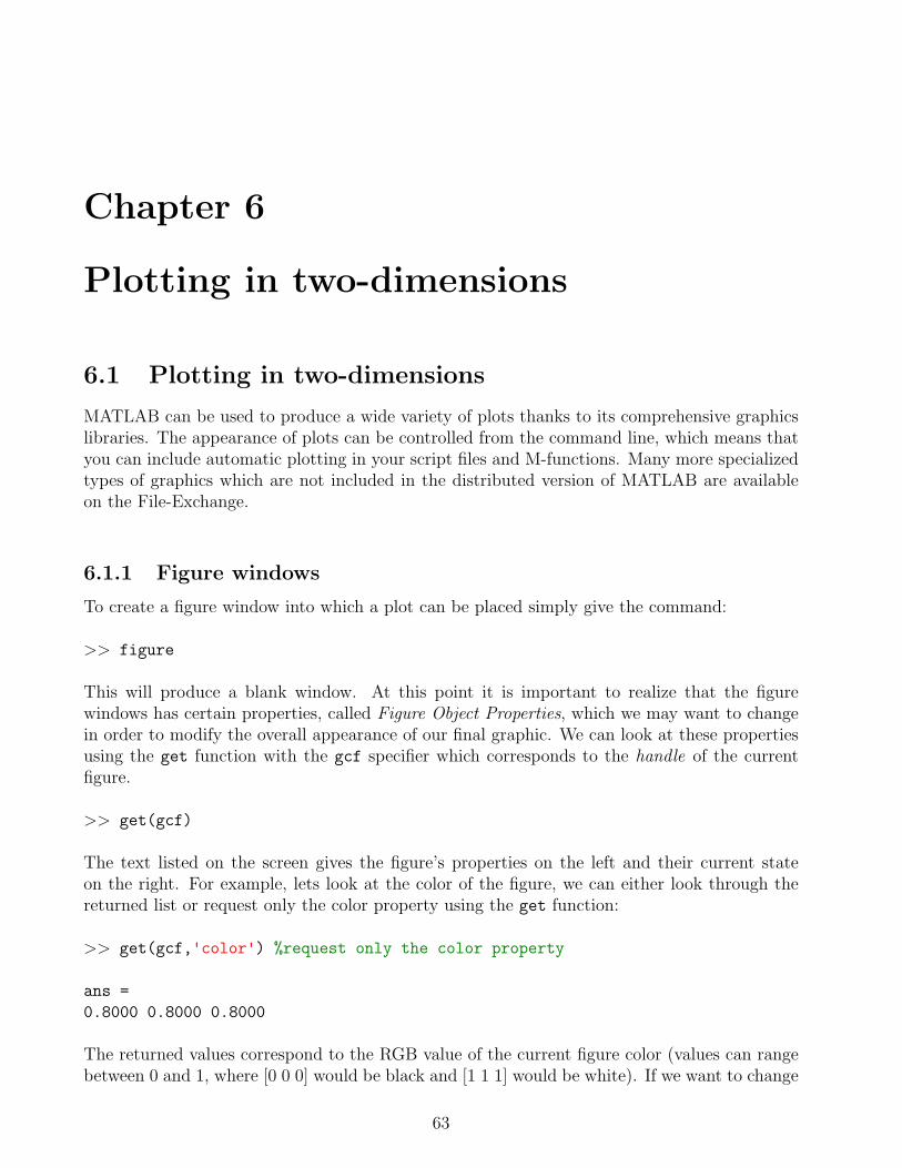
Chapter 6
Plotting in two-dimensions
6.1 Plotting in two-dimensions
MATLAB can be used to produce a wide variety of plots thanks to its comprehensive graphicslibraries. The appearance of plots can be controlled from the command line, which means thatyou can include automatic plotting in your script files and M-functions. Many more specializedtypes of graphics which are not included in the distributed version of MATLAB are availableon the File-Exchange.
6.1.1 Figure windows
To create a figure window into which a plot can be placed simply give the command:
>> figure
This will produce a blank window. At this point it is important to realize that the figurewindows has certain properties, called Figure Object Properties, which we may want to changein order to modify the overall appearance of our final graphic. We can look at these propertiesusing the get function with the gcf specifier which corresponds to the handle of the currentfigure.
>> get(gcf)
The text listed on the screen gives the figure’s properties on the left and their current stateon the right. For example, lets look at the color of the figure, we can either look through thereturned list or request only the color property using the get function:
>> get(gcf,'color') %request only the color property
ans =
0.8000 0.8000 0.8000
The returned values correspond to the RGB value of the current figure color (values can rangebetween 0 and 1, where [0 0 0] would be black and [1 1 1] would be white). If we want to change
63

the color of the figure, for example to red we use the set function and provide the appropriatecolor vector (in this case [1 0 0]):
>> set(gca,'color',[1 0 0]) %reset the color property
Now when you look at the figure it should be red (a set of axes may also have appeared).MATLAB figures and plots are all controlled by adjusting the properties of the handles, just asin the example we performed.
6.1.2 Using Handles
At first the use of handles can seem like a very complicated way of controlling the appearanceof graphics compared to software such as EXCEL where you just need to double-click to changeitems. The advantage of using handles is that we can include adjustments to our figures andplots in script files, so with a bit of programming the appearance of a graphic can be optimizedautomatically. Understanding and using handles takes some time, especially remembering thespecific property names which you may want to adjust. Over time you will remember theimportant handle properties and for the more obscure ones the MATLAB help system can tellyou what they do and how they can be adjusted. Throughout the following examples we willbe using handles to modify graphics, so it is important to be familiar with the following simplespecifiers.
• gcf specifies the current figure handle
• gca specifies the current axes handle
• gco specifies the current graphic object handle
6.2 Simple data plotting
Now we’ll generate some simple x,y data and then plot it using the plot function:
>> t = linspace(0,3*pi,30); %30 point equally spaced vector between 0 and 3pi
>> x = sqrt(t).*cos(t); %calculate the x values
>> y = sqrt(t).*sin(t); %calculate the y values
>> figure %create a new figure window
>> plot(x,y) %plot the x,y data
64

−4 −3 −2 −1 0 1 2 3−3
−2
−1
0
1
2
3
Figure 6.1: A simple two-dimensional plot of x,y data.
The plot function has a number of additional arguments that allow us to control the styleof the plotted line. For example if we wanted to plot the line in red we would use the additionaloption:
>> plot(x,y,'r') %plot the x,y data in red
You should now see that the plot uses a red line. We can also specify plot symbols ratherthan a line, for example open circles in green:
>> plot(x,y,'og') %plot the x,y data as green open circles
or small closed symbols in black:
>> plot(x,y,'.k') %plot the x,y data as black points
or diamond symbols (specified using 'd') in magenta with a connecting line:
>> plot(x,y,'dm-') %plot the x,y data as magenta diamonds with a line
or the same as above with a dashed line:
>> plot(x,y,'dm--') %plot the x,y data as magenta diamonds with a dashed line
As mentioned above, you will memorize these various specifiers with time, but they are alllisted in the MATLAB help so it is very easy to find them. If we want to store the handle forthe plotted line we need to provide an output variable for the plot function, we can then viewthe handle using get and modify its properties with set.
>> h=plot(x,y,'dm--') %output the handle as h
>> get(h)
65

Listed on the screen you’ll see the properties of the plotted data, for example you can seethe LineStyle is '--' just as it was set in the plot command and the Marker is 'diamond'.As an example of modifying the handle we’ll set the color to red, the symbols to squares, thesize of the symbols to 12 points, the lines to be dot-dashed and to have a thickness of 2 points.
>> set(h,'color',[1 0 0]) %set the color to red
>> set(h,'marker','square') %set the symbols as squares
>> set(h,'markersize',12) %set the symbol size to 12 pts
>> set(h,'linestyle','-.') %set the line to dot-dashed
>> set(h,'linewidth',2) %set the line thickness to 2 pts
−4 −3 −2 −1 0 1 2 3−3
−2
−1
0
1
2
3
Figure 6.2: A two-dimensional plot of x,y data, the appearance of which has been changed usingits handle.
At anytime we can plot additional data onto the graphic. Now we’ll generate a second dataset and add it to the plot.
>> x1=-y; %create a new x array
>> y1=-x; %create a new y array
>> h1=plot(x1,y1,'g') %plot the data as a green line with the handle h1
When we look at the figure we can see that there is a problem, the old line has been re-moved from the plot and replaced with the new line. If we want to show both lines on the sameplot we need to use the hold on command, which tells MATLAB to add data to the graphicrather than replacing it.
>> h0=plot(x,y,'k') %plot the data as a black line with the handle h0
>> hold on %tells MATLAB we want to add to the plot
>> h1=plot(x1,y1,'g') %plot the data as a green line with the handle h1
66

−4 −3 −2 −1 0 1 2 3−3
−2
−1
0
1
2
3
4
Figure 6.3: The two sets of x,y data plotted together using the hold on command.
We also have handles for each plotted data set, h0 and h1, so we could modify either of thelines using the set command.
6.2.1 Modifying the axes
So far we have used the handles of the plotted lines to change their appearance, but we canalso take a similar approach with the appearance of the axes. There are some simple commandswhich allow us to add labels and a title, which must be defined as character strings.
>> xlabel('X data') %add a text string to the x-axis
>> ylabel('Y data') %add a text string to the x-axis
>> title('Two spirals demonstrating the plot command') %add a title
−4 −3 −2 −1 0 1 2 3−3
−2
−1
0
1
2
3
4
X data
Y d
ata
Two spirals demonstrating the plot command
Figure 6.4: The two sets of x,y data plotted with axis labeling and a title.
We can access the handle for the axes using the gca identifier.
67

>> get(gca)
As you can see there are a large number of properties and we can change any of them using theset command. As with the other handles it is important to check the MATLAB documentationto find what the allowable states for any given property are. The following sets of commandsshow some of the properties that can be changed, enter them one by one each time checkingthe figure to see how things have changed.
>> set(gca,'tickdir','out') %tick marks point outwards rather than inwards
>> set(gca,'yminortick','on') %plot intermediate ticks on the y-axis
>> set(gca,'fontsize',16) %set the text size to 16 points
>> set(gca,'xdir','reverse') %reverse the direction of the x-axis
>> set(gca,'ylim',[-2 2]) % set the y-axis range as -2 to 2
>> set(gca,'yaxislocation','right') %place the y-axis on the right hand side
>> set(gca,'xgrid','on') %plot a grid over the x-axis
>> set(gca,'fontangle','italic') %use italic fonts
>> set(gca,'xtick',[-4 -2 0 1 2.5 3.7]) %plot xticks at specific values
−4−2012.53.7−2
−1
0
1
2
X data
Y d
ata
Two spirals demonstrating the plot command
Figure 6.5: The two sets of x,y data plotted with a collection of modifications to the axes.
As you can see you can change every aspect of a graphic using the handles, all you need toknow is the name of the property you want to change.
6.2.2 Multiple sets of axes in a single figure
Often you will want to plot and compare a number data sets within a single figure window, thiscan be done using the axes command or its extension subplot. When we create a new figurewindow we can place axes in a specific position with a specific size. The axes command has4 numerical inputs entered as a position vector axes('position', RECT), where RECT = [left,bottom, width, height] specifies the location and size of the side of the axis box, relative to thelower-left corner of the Figure window, in normalized units where (0,0) is the lower-left corner
68

and (1.0,1.0) is the upper-right. In this first example we’ll make a figure with two sets of axesand plot our spiral data separately.
>> close all %close the existing figure windows
>> figure %create a new figure window
Now we’ll form a set of axes which have their bottom left corner located at (0.1,0.2) a width of0.3 and a height of 0.7. We’ll then plot the x,y data inside the axes.
>> axes('position',[0.1 0.2 0.3 0.7]) %create specific axes
>> plot(x,y,'b') %plot x and y in blue
Lets add a second set of axes which have there bottom left corner located at (0.5,0.4) a widthof 0.4 and a height of 0.2. Then we’ll plot the data set x1,y1 inside the axes.
>> axes('position',[0.5 0.4 0.4 0.2]) %create specific axes
>> plot(x1,y1,'r') %plot x1 and y1 in red
−4 −2 0 2 4−3
−2
−1
0
1
2
3
−4 −2 0 2 4−5
0
5
Figure 6.6: User specified axes within a single figure window.
If you would like to create a set of regularly sized and spaced axes then you can use thesubplot command. subplot requires 3 inputs, the number of rows of axes, the number ofcolumns of axes and which set of axes it should make active. This may sound confusing buthopefully the example will make things clear, we’ll construct 6 sets of axes in a grid with 2rows and 3 columns. When we specify the active axes (the third input of subplot) they arenumbered in a sequence which runs from left to right along each row from top to bottom. Todemonstrate this concept we’ll use the axes out of their natural sequence. Remember to keeplooking at the figure to see how it evolves with each command.
>> close all %close the existing figure windows
>> figure %create a new figure window
>> subplot(2,3,1) %2 rows & 3 columns of axes, use position 1
69
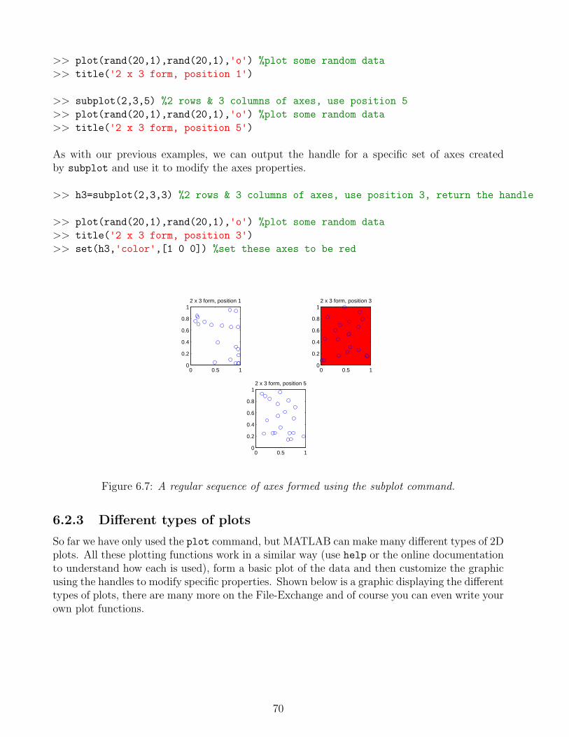
>> plot(rand(20,1),rand(20,1),'o') %plot some random data
>> title('2 x 3 form, position 1')
>> subplot(2,3,5) %2 rows & 3 columns of axes, use position 5
>> plot(rand(20,1),rand(20,1),'o') %plot some random data
>> title('2 x 3 form, position 5')
As with our previous examples, we can output the handle for a specific set of axes createdby subplot and use it to modify the axes properties.
>> h3=subplot(2,3,3) %2 rows & 3 columns of axes, use position 3, return the handle
>> plot(rand(20,1),rand(20,1),'o') %plot some random data
>> title('2 x 3 form, position 3')
>> set(h3,'color',[1 0 0]) %set these axes to be red
0 0.5 10
0.2
0.4
0.6
0.8
12 x 3 form, position 1
0 0.5 10
0.2
0.4
0.6
0.8
12 x 3 form, position 5
0 0.5 10
0.2
0.4
0.6
0.8
12 x 3 form, position 3
Figure 6.7: A regular sequence of axes formed using the subplot command.
6.2.3 Different types of plots
So far we have only used the plot command, but MATLAB can make many different types of 2Dplots. All these plotting functions work in a similar way (use help or the online documentationto understand how each is used), form a basic plot of the data and then customize the graphicusing the handles to modify specific properties. Shown below is a graphic displaying the differenttypes of plots, there are many more on the File-Exchange and of course you can even write yourown plot functions.
70

Figure 6.8: The various 2D plot types available in MATLAB
6.2.4 Contour plots
One specific type of plot that as geoscientists we must pay attention to is the contour plot.MATLAB has inbuilt functions to plot contour maps, but at a first glance the form of theinput data can appear to be a bit confusing. To contour spatial data we must of course havetwo location coordinates, for example latitude and longitude, and some measured parametersuch as sea-surface temperate. Most often we collect these kind of data as a series of [x,y,z]triplets, forming three columns of data. Unfortunately MATLAB does not follow this system(not surprisingly we need to use a matrix form for data input), so we have to perform somepreprocessing before we can contour data. As an example of the form in which MATLAB canplot x,y,z data we’ll use peaks which is a function of two variables, obtained by translating andscaling Gaussian distributions. We’ll generate and plot the peaks function for 20 x 20 data grids.
>> clear all, close all
>> n=20; %number of grid points
>> [x,y,z]=peaks(n); %evaluate peaks on a 20 x 20 grid
>> size(x) %we can see the size of x
ans =
20 20
>> contour(x,y,z,10) %plot data with 10 contours
>> colorbar %add a colorbar to show the z values
71
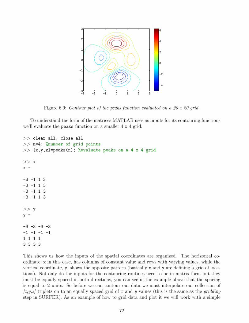
−3 −2 −1 0 1 2 3−3
−2
−1
0
1
2
3
−4
−2
0
2
4
6
Figure 6.9: Contour plot of the peaks function evaluated on a 20 x 20 grid.
To understand the form of the matrices MATLAB uses as inputs for its contouring functionswe’ll evaluate the peaks function on a smaller 4 x 4 grid.
>> clear all, close all
>> n=4; %number of grid points
>> [x,y,z]=peaks(n); %evaluate peaks on a 4 x 4 grid
>> x
x =
-3 -1 1 3
-3 -1 1 3
-3 -1 1 3
-3 -1 1 3
>> y
y =
-3 -3 -3 -3
-1 -1 -1 -1
1 1 1 1
3 3 3 3
This shows us how the inputs of the spatial coordinates are organized. The horizontal co-ordinate, x in this case, has columns of constant value and rows with varying values, while thevertical coordinate, y, shows the opposite pattern (basically x and y are defining a grid of loca-tions). Not only do the inputs for the contouring routines need to be in matrix form but theymust be equally spaced in both directions, you can see in the example above that the spacingis equal to 2 units. So before we can contour our data we must interpolate our collection of[x,y,z] triplets on to an equally spaced grid of x and y values (this is the same as the griddingstep in SURFER). As an example of how to grid data and plot it we will work with a simple
72

topographic data set which is stored in the file dmap.mat with the variables x, y and z.
>> clear all, close all
>> load dmap %load the data file
>> plot(x,y,'or') %plot the positions of the measured data points
>> xlabel('x coordinate') %label the x axis
>> ylabel('y coordinate') %label the y axis
0 1 2 3 4 5 6 70
1
2
3
4
5
6
7
x coordinate
y co
ordi
nate
Figure 6.10: Positions of the data points in the dmap data set
The first thing to note is that our data is in columns not matrices and that the points werenot measured on a regular grid. Now we must create some regular grids onto which we caninterpolate the data. To do this we’ll use the meshgrid function which takes equally spacedvectors and forms them into grids.
>> xi=[0:0.25:6.5]; %equally spaced row vector of x positions
>> yi=[0:0.25:6.5]; %equally spaced column vector of y positions
>> [xi grid,yi grid]=meshgrid(xi,yi);
>> plot(xi grid,yi grid,'.k') %plot the grid positions
73

0 1 2 3 4 5 6 70
1
2
3
4
5
6
7
x coordinate
y co
ordi
nate
Figure 6.11: Positions of the data points in the dmap data set (red circles) with the new positionsforming the regular grids (black dots)
We can now see the positions of the regular spaced grid points and our final task is to interpo-late our topographic data onto these new grids (we’ll discussed interpolation in detail later in thecourse). To perform the interpolation we use the function griddata, giving our measured datax, y and z and the uniform grids x grid and y grid onto which the data should be interpolated.
>> zi grid=griddata(x,y,z,xi grid,yi grid); %interpolate the z data
>> hold on
>> contour(xi grid,yi grid,zi grid,10) %plot 10 contour lines
0 1 2 3 4 5 6 70
1
2
3
4
5
6
7
x coordinate
y co
ordi
nate
Figure 6.12: Contours determined from the data points in the dmap data set (red circles) afterinterpolation onto the new positions in the regular grids (black dots)
There are a variety of different contour-type maps available, for example contourf will pro-duce a filled contour map and pcolor plots a colored grid. Try the following examples (note
74

that MATLAB does not extrapolate the data so some regions of the maps will be empty, againwe’ll talk about this later).
>> figure
>> contourf(xi grid,yi grid,zi grid,10) %plot 10 filled contour intervals
>> figure
>> pcolor(xi grid,yi grid,zi grid) %pseudocolor plot
6.2.5 Saving and exporting figures
MATLAB figures can be saved from the drop-down menu in the specific figure window. Thismeans you can reload figures and continue working on them at a later time. You can also exportthe figures from the drop-down menu into various graphic formats. I’ve always found it usefulto export figures as encapsulated postscript (*.eps), which can then be imported into softwaresuch as CorelDraw and modified (encapsulated postscript produces vector graphics).
6.3 Exercise: Life’s ups and downs in the Logistic Map
In this exercise we’ll combine a number of techniques that we have studied in the course sofar to generate a data set and produce a high quality plot of the final output. If you image apopulation within an enclosed environment, for example goldfish in a garden pond, there are anumber of factors which will control how the population grows or shrinks from one generationto the next. For example:
• Food supply
• Sexual reproduction
• Disease
• Predation
• Competition with other species
• ... and many more
A number of simple theories have been formulated to consider how the population will changefrom one generation to the next, but they rely on unrealistic assumptions such as unlimited foodsupply and free reproduction. When ecologists studied real animal populations they found anumber of different patterns as a function of time. Using a value of 1 to represent the maximumpossible population and 0 to represent extinction, three basic patterns of “stable”, “periodic”and “random” behavior were defined.
75

Figure 6.13: A “stable” population moves towards a constant equilibrium value. Alternatively,“periodic” populations oscillate between two or more values. Finally “random” populationsreveal no coherent pattern.
Ecologists believed that two possible mechanisms could have been responsible for the ob-served patterns. If the population is in equilibrium with the environment then “stable” and“periodic” patterns could be expected. However if the population is heavily influenced by un-predictable environmental factors the behavior of “random” populations could be explained.These two systems are however very different, so which is correct?
In the 1950’s ecologists developed the so-called “logistic equation”, which was designed tomodel population behavior, it contains a term to express population growth from one generationto the next and a second term which restricts the population when it becomes too large.
xnext = r ∗ xinitial ∗ (1− xinitial) (6.1)
where xinitial is this year’s population, xnext is next year’s population and r is the “biotic po-tential”. The biotic potential influences how much the population changes from one generationto the next, it will be controlled by factors such as food supply, competition, etc. The term(1−xinitial) keeps the growth within the defined limits because as x increases, (1−x) decreases.Some key features of the logistic equation are:
• When x is low the population grows rapidly.
• At intermediate levels of x the population growth is almost zero.
• At high levels of x the population crashes.
Using the logistic equation is is possible to produce “stable”, “periodic” and “random” behaviorsimply by changing the constant, r, in the equation, therefore we have one mechanism to describeall three types of behavior. With increasing computing power, it became possible to study thedynamics of the Logistic equation. The investigation is very simple.
76
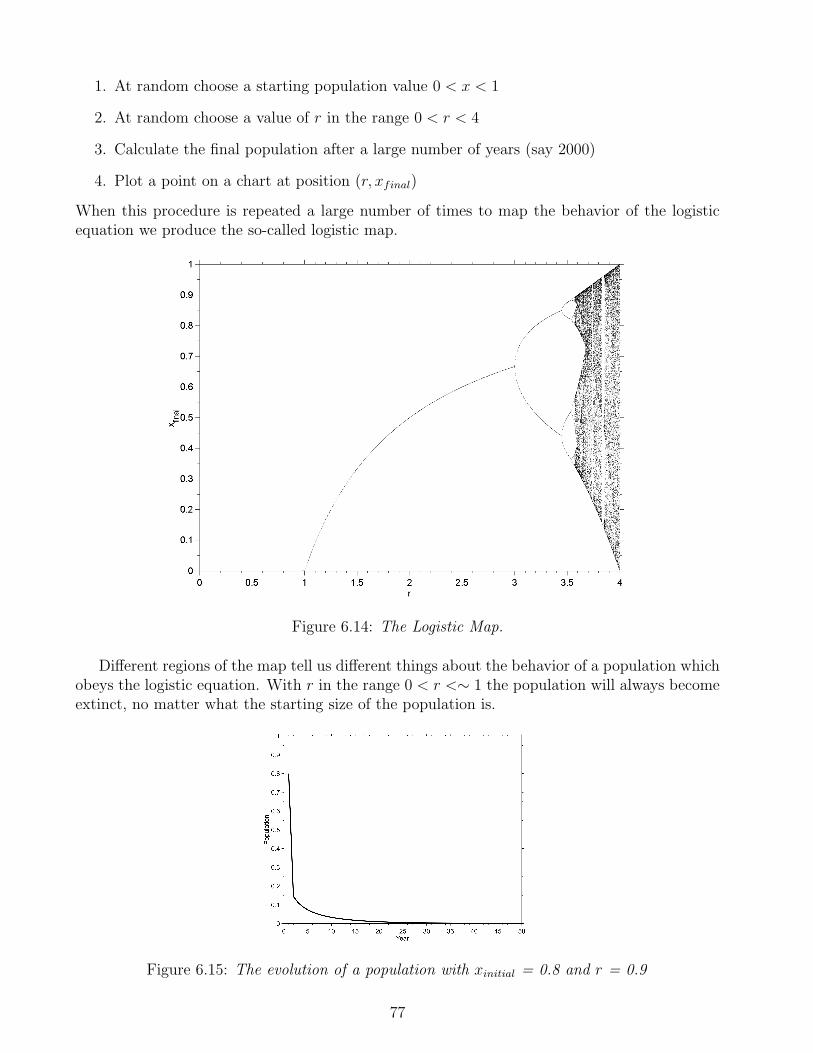
1. At random choose a starting population value 0 < x < 1
2. At random choose a value of r in the range 0 < r < 4
3. Calculate the final population after a large number of years (say 2000)
4. Plot a point on a chart at position (r, xfinal)
When this procedure is repeated a large number of times to map the behavior of the logisticequation we produce the so-called logistic map.
Figure 6.14: The Logistic Map.
Different regions of the map tell us different things about the behavior of a population whichobeys the logistic equation. With r in the range 0 < r <∼ 1 the population will always becomeextinct, no matter what the starting size of the population is.
Figure 6.15: The evolution of a population with xinitial = 0.8 and r = 0.9
77

With r in the range ∼ 1 < r <∼ 3 the population reaches a steady single value no matterwhat the starting value of xinitial is.
Figure 6.16: The evolution of a population with xinitial = 0.02 and r = 2.5
With r in the range ∼ 3 < r <∼ 3.42 the population shifts between two values. This iscalled “period two” behavior.
Figure 6.17: The evolution of a population with xinitial = 0.02 and r = 3.25
With r in the range ∼ 3.42 < r <∼ 3.57 the population shifts between four values. This iscalled “period four” behavior.
78
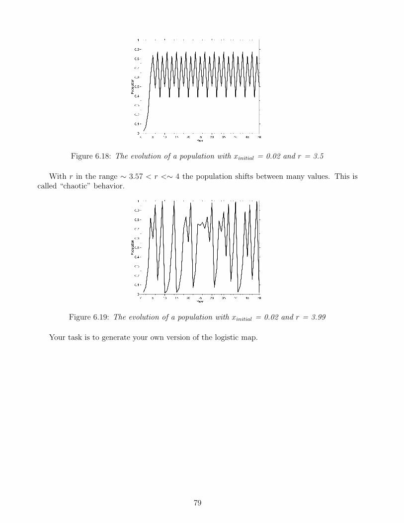
Figure 6.18: The evolution of a population with xinitial = 0.02 and r = 3.5
With r in the range ∼ 3.57 < r <∼ 4 the population shifts between many values. This iscalled “chaotic” behavior.
Figure 6.19: The evolution of a population with xinitial = 0.02 and r = 3.99
Your task is to generate your own version of the logistic map.
79

Steps to completing the exercise
This exercise will require a number of different steps.
• Generate code to iterate the logistic equation from a given starting point for agiven number of time steps.
• Simulate a large number of populations with different values of r and xinitial.
• Extract data from your model runs to form a plot of the logistic map.
• Use your plotting skills to make a nice version of the logistic map.
The simplest way to approach this problem is to write a script which will allow youto generate one time series and then extend the code to run from multiple startingpoints. To run for a single value of r and xinitial:
1. Generate a random number between 0 and 1 to provide xinitial.
2. Generate a random number between 0 and 4 to provide r.
3. Use a for loop to iterate the logistic equation 2000 times, updating the popula-tion after each iteration.
4. Find the final value of the population after 2000 iterations, this will give you onepoint (r,xfinal) for the logistic map.
Once you have a method for finding a single point you can then repeat it thousandsof times to find a collection of xfinal values for different values of r and xinitial.
Functions you may find useful
• rand - Uniformly distributed pseudo-random numbers.
80

Chapter 7
Plotting in three-dimensions
7.1 Plotting in three-dimensions
Three-dimensional graphics are a natural extension of the two-dimensional graphics we studiedearlier. We can plot data points and lines in three-dimensional space using the function plot3.It is also possible to plot surfaces and meshes, where the data input must be on regular grids,which means interpolation of your data may be necessary. As with the two-dimensional graphicsthe appearance of the three-dimensional plots is controlled via the graphic handles.
Figure 7.1: The various 3D plot types available in MATLAB
81
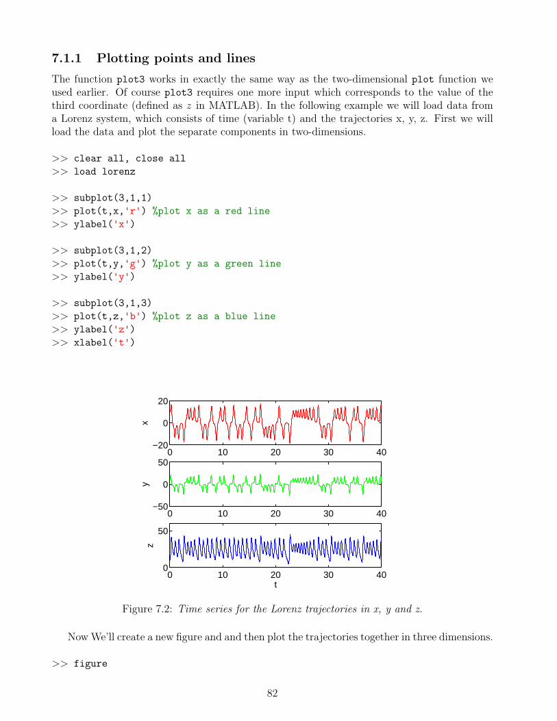
7.1.1 Plotting points and lines
The function plot3 works in exactly the same way as the two-dimensional plot function weused earlier. Of course plot3 requires one more input which corresponds to the value of thethird coordinate (defined as z in MATLAB). In the following example we will load data froma Lorenz system, which consists of time (variable t) and the trajectories x, y, z. First we willload the data and plot the separate components in two-dimensions.
>> clear all, close all
>> load lorenz
>> subplot(3,1,1)
>> plot(t,x,'r') %plot x as a red line
>> ylabel('x')
>> subplot(3,1,2)
>> plot(t,y,'g') %plot y as a green line
>> ylabel('y')
>> subplot(3,1,3)
>> plot(t,z,'b') %plot z as a blue line
>> ylabel('z')
>> xlabel('t')
0 10 20 30 40−20
0
20
x
0 10 20 30 40−50
0
50
y
0 10 20 30 400
50
z
t
Figure 7.2: Time series for the Lorenz trajectories in x, y and z.
Now We’ll create a new figure and and then plot the trajectories together in three dimensions.
>> figure
82
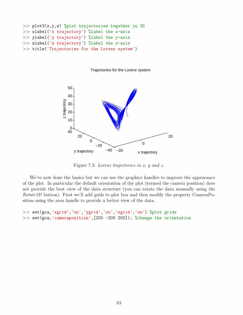
>> plot3(x,y,z) %plot trajectories together in 3D
>> xlabel('x trajectory') %label the x-axis
>> ylabel('y trajectory') %label the y-axis
>> zlabel('z trajectory') %label the z-axis
>> title('Trajectories for the Lorenz system')
−20
0
20
−40−20
020
400
10
20
30
40
50
x trajectory
Trajectories for the Lorenz system
y trajectory
z tr
ajec
tory
Figure 7.3: Lorenz trajectories in x, y and z.
We’ve now done the basics but we can use the graphics handles to improve the appearanceof the plot. In particular the default orientation of the plot (termed the camera position) doesnot provide the best view of the data structure (you can rotate the data manually using theRotate3D button). First we’ll add grids to plot box and then modify the property CameraPo-sition using the axes handle to provide a better view of the data.
>> set(gca,'xgrid','on','ygrid','on','zgrid','on') %plot grids
>> set(gca,'cameraposition',[200 -200 200]); %change the orientation
83

−20−10
010
20 −40−20
020
40
0
10
20
30
40
50
y trajectory
Trajectories for the Lorenz system
x trajectory
z tr
ajec
tory
Figure 7.4: Lorenz trajectories in x, y and z, plotted with grids and rotated to provide a clearview of the data. Note the values for the CameraPosition were obtained by gradual modificationuntil a satisfactory position was found.
7.1.2 Surface plots
Earlier we used two-dimensional contour maps to represent topographic data, but MATLABalso has the capacity to represent such data in a three-dimensional manner using surfaces andmeshes. As with our contour data the input for such plots must be composed of regular grids,so we need to preprocess our data using meshgrid and griddata.
>> clear all, close all
>> load dmap %load the data file
>> xi=[0:0.25:6.5]; %equally spaced row vector of x positions
>> yi=[0:0.25:6.5]; %equally spaced column vector of y positions
>> [xi grid,yi grid]=meshgrid(xi,yi);
>> zi grid=griddata(x,y,z,xi grid,yi grid); %interpolate the z data
Now we’ll create a surface plot of the data, add the original data on top, rotate the surfaceand make it slightly transparent. Feel free to experiment with the handle of the surface (whichwill be called hs) to see what effects you can create.
>> h=surf(xi grid,yi grid,zi grid) %create a surface plot
>> hold on %add to the plot
>> hs = plot3(x,y,z,'ok','markerfacecolor','k') %original data points
>> set(h,'facealpha',0.5) %surface is semitransparent
>> xlabel('x') %label the x-axis
>> ylabel('y') %label the y-axis
>> zlabel('Height') %label the z-axis
>> set(gca,'cameraposition',[-21.5 44.2 2691]) %rotate the plot
84

>> colorbar %add a colorbar
Figure 7.5: Topographic data set plotted as a surface.
By default MATLAB uses a sequences of colors, termed a colormap, which runs from bluethrough to red. However there are others to choose from and you can even create your own,for example there is an inbuilt colormap called gray which uses a grayscale, this can be imple-mented in the current figure using the colormap command.
>> colormap gray
Figure 7.6: Topographic data set plotted as a surface with the gray colormap.
85
There are a variety of different ways in which we could have represented the topographicdata in the example, see figure 7.1
7.1.3 Overlaying images
To demonstrate the flexibility of the graphics routines in MATLAB we’ll now look at a morecomplicated example, that involves plotting a satellite image of the earth on top of a sphere.We will read the satellite image (in the form of a jpg) directly from a internet location and storeit as a matrix.
>> clear all, close all
>> filename = 'http://veimages.gsfc.nasa.gov/2430/land ocean ice 2048.jpg';
>> cdata = imread(filename); %read the image from the given location
>> size(cdata) %size of the image data
ans =
1024 2048 3
Note that the size of the image data is 1024 rows (latitude), 2048 columns (longitude) and3 layers. Each layer provides information on a given color channel, red, green and blue. Nowwe will produce a collection of data points which lie on a sphere, which will form the basis ofour Earth:
>> [x, y, z] = sphere(72); %generate data points on a sphere
>> figure %open a new figure window
>> h = surf(x,y,z) %plot a surface from the sphere data
>> axis vis3d %set the axis perspective suitable for 3D
86
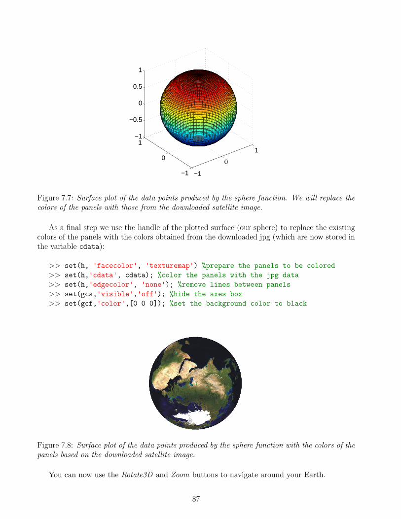
−1
0
1
−1
0
1−1
−0.5
0
0.5
1
Figure 7.7: Surface plot of the data points produced by the sphere function. We will replace thecolors of the panels with those from the downloaded satellite image.
As a final step we use the handle of the plotted surface (our sphere) to replace the existingcolors of the panels with the colors obtained from the downloaded jpg (which are now stored inthe variable cdata):
>> set(h, 'facecolor', 'texturemap') %prepare the panels to be colored
>> set(h,'cdata', cdata); %color the panels with the jpg data
>> set(h,'edgecolor', 'none'); %remove lines between panels
>> set(gca,'visible','off'); %hide the axes box
>> set(gcf,'color',[0 0 0]); %set the background color to black
Figure 7.8: Surface plot of the data points produced by the sphere function with the colors of thepanels based on the downloaded satellite image.
You can now use the Rotate3D and Zoom buttons to navigate around your Earth.
87

7.2 Exercise: Plotting elevation data
In the file Hawaii.mat you’ll find bathymetric and topographic data for region around the mainHawaiian Islands. The data represent a scatter of latitude and longitude points with theirrespective height data. The aim of this exercise is to produce regular latitude and longitudegrids onto which the height data can be interpolated and then to plot surfaces which representthe topography and bathymetry.
1. Grid the data at a resolution of 0.1o for both the longitude and the latitude.
2. Plot the gridded data using a suitable 3D plot, add appropriate labels etc.
3. Plot a version of the data that includes the points above sea-level and has a height of zeroeverywhere else.
4. Plot a version of the data that includes the points below sea-level and has a height of zeroeverywhere else.
88

Steps to completing the exercise
This exercise requires a number of steps which follow the previous examples in thischapter, creating surfaces which represent the bathymetry and topography can beachieved using relational operators. The basic steps of the exercise are as follows:
• Load the data file Hawaii.mat which contains the variables latitude, longitudeand elevation.
• Create a regular array of latitudes between the minimum and maximum valuesin the data set with a spacing of 0.1o.
• Create a regular array of longitudes between the minimum and maximum valuesin the data set with a spacing of 0.1o.
• Produce regular grids of latitude and longitude from the prepared arrays.
• Interpolate the height data onto the regular position grids.
• Create a copy of the interpolated data with all the values less than zero replacedwith zeros. This data can be plotted as a surface representing the topography.
• Create a copy of the interpolated data with all the values greater than zeroreplaced with zeros. This data can be plotted as a surface representing thebathymetry.
Functions you may find useful
• min - Smallest elements in array.
• max - Largest elements in array.
• meshgrid - Generate X and Y arrays for 3-D plots.
• griddata - Data gridding.
• find - Find indices of elements which meet relational criteria.
• surf - 3-D shaded surface plot.
• xlabel - Label x-axis.
• ylabel - Label y-axis.
• zlabel - Label z-axis.
89
Chapter 8
Interpolation
Interpolation is a method by which we can use data points to estimate the unknown value ofa function at a given location. This is a common problem in the geosciences, for example, ifwe have a collection of calibrated radiocarbon ages through a sediment core, how can we esti-mate the age of the sediment at any given depth? MATLAB has inbuilt functions to performinterpolation in any given number of dimensions, they are easy to use but it is important toappreciate that the various options you can select from can strongly influence your results.
8.1 Interpolation in one dimension
This is the simplest form of interpolation, estimating a value y′ for a given value of x′ basedon a collection of known x, y data points. As an example of the different methods available inMATLAB we will load an x, y data series and perform different interpolation tasks.
>> clear all %clear MATLAB’s memory
>> close all %close all figures
>> load bedf %load the x,y data
>> plot(x,y,'.r') %plot the data as red points
>> xlabel('x'), ylabel('y') %label the axes
90
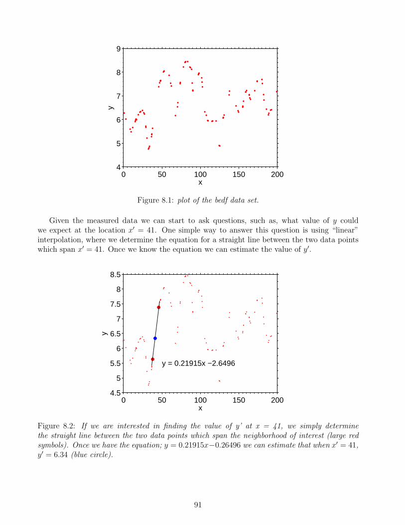
0 50 100 150 2004
5
6
7
8
9
x
y
Figure 8.1: plot of the bedf data set.
Given the measured data we can start to ask questions, such as, what value of y couldwe expect at the location x′ = 41. One simple way to answer this question is using “linear”interpolation, where we determine the equation for a straight line between the two data pointswhich span x′ = 41. Once we know the equation we can estimate the value of y′.
0 50 100 150 2004.5
5
5.5
6
6.5
7
7.5
8
8.5
y = 0.21915x −2.6496
x
y
Figure 8.2: If we are interested in finding the value of y’ at x = 41, we simply determinethe straight line between the two data points which span the neighborhood of interest (large redsymbols). Once we have the equation; y = 0.21915x−0.26496 we can estimate that when x′ = 41,y′ = 6.34 (blue circle).
91
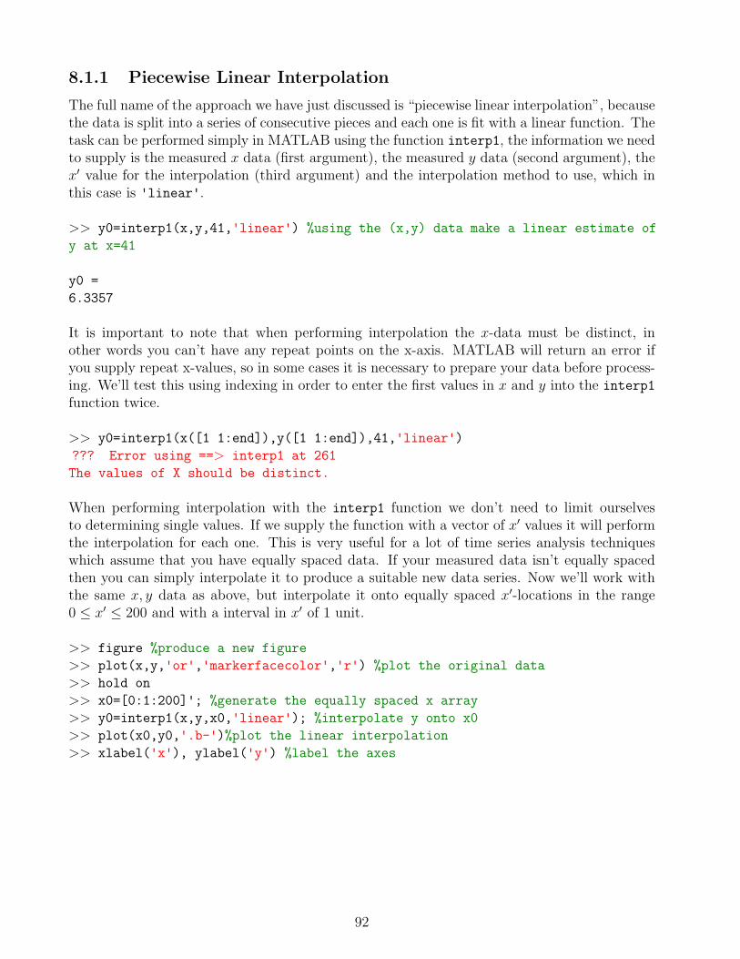
8.1.1 Piecewise Linear Interpolation
The full name of the approach we have just discussed is “piecewise linear interpolation”, becausethe data is split into a series of consecutive pieces and each one is fit with a linear function. Thetask can be performed simply in MATLAB using the function interp1, the information we needto supply is the measured x data (first argument), the measured y data (second argument), thex′ value for the interpolation (third argument) and the interpolation method to use, which inthis case is 'linear'.
>> y0=interp1(x,y,41,'linear') %using the (x,y) data make a linear estimate of
y at x=41
y0 =
6.3357
It is important to note that when performing interpolation the x-data must be distinct, inother words you can’t have any repeat points on the x-axis. MATLAB will return an error ifyou supply repeat x-values, so in some cases it is necessary to prepare your data before process-ing. We’ll test this using indexing in order to enter the first values in x and y into the interp1
function twice.
>> y0=interp1(x([1 1:end]),y([1 1:end]),41,'linear')
??? Error using ==> interp1 at 261
The values of X should be distinct.
When performing interpolation with the interp1 function we don’t need to limit ourselvesto determining single values. If we supply the function with a vector of x′ values it will performthe interpolation for each one. This is very useful for a lot of time series analysis techniqueswhich assume that you have equally spaced data. If your measured data isn’t equally spacedthen you can simply interpolate it to produce a suitable new data series. Now we’ll work withthe same x, y data as above, but interpolate it onto equally spaced x′-locations in the range0 ≤ x′ ≤ 200 and with a interval in x′ of 1 unit.
>> figure %produce a new figure
>> plot(x,y,'or','markerfacecolor','r') %plot the original data
>> hold on
>> x0=[0:1:200]'; %generate the equally spaced x array
>> y0=interp1(x,y,x0,'linear'); %interpolate y onto x0
>> plot(x0,y0,'.b-')%plot the linear interpolation
>> xlabel('x'), ylabel('y') %label the axes
92

0 50 100 150 2004
5
6
7
8
9
x
y
Figure 8.3: Linear interpolation of unequally spaced x,y data onto a new equally spaced x vector.
When we examine the interpolated values we discover that for locations at the start and endof the interpolated data MATLAB has returned NaN (Not a Number), rather than a real number.
>> [x0(1:3),y0(1:3)] %list the first 3 values of the interpolated data
ans =
0 NaN
1.0000 6.2677
2.0000 6.1500
>> x(1:3) %the first value of the x input data
ans =
0.9268
3.0807
8.6048
We can now see that the interpolation at x′ = 0 is not possible because it is outside therange of our input data. We can attempt to overcome this problem using extrapolation, whichmakes the assumption that the properties at the edges of the x,y data continue unmodifiedoutside the measured range. Applying extrapolation to interp1 is simple, but as we will seelater the results have to be treated with extreme caution.
>> y0=interp1(x,y,x0,'linear','extrap'); %add a 5th option to perform extrapolation
>> [x0(1:3),y0(1:3)] %we now have predicted y-values outside of the measured x-range
93
ans =
0 6.3854
1.0000 6.2677
2.0000 6.1500
So far we have only looked at linear interpolation, which assumes that the gaps between datapoints can be connected by straight lines. There are however a number of different approachesbuilt into interp1 that we can use for interpolation and they all give different results! It isimportant to realize at this stage there is no single correct method with which to approachinterpolation, each method does different things depending on how it is designed. All the meth-ods are “wrong” in so far as (unless we are very lucky) they will not predict y′ correctly, butthey are wrong in different ways depending on their methodology. The best we can do is tryto choose the method of interpolation which is most suitable for the type of data set we areworking with.
8.1.2 Nearest Neighbor Interpolation
The nearest neighbor method is probably the simplest approach to interpolation. If we areinterested in the value of y′ at a location x′ we simply search for the measured data point whichhas the x-value closest to our point of interest and assign y′ to the same value as this data point.We will work again with the bedf data from the previous example.
>> y0=interp1(x,y,x0,'nearest'); %interpolate y onto x0 using the nn approach
>> figure %produce a new figure
>> plot(x,y,'or','markerfacecolor','r') %plot the original data
>> xlabel('x'), ylabel('y') %label the axes
>> hold on
>> plot(x0,y0,'.g-') %plot the nearest-neighbor interpolation
>> title('Nearest neighbor interpolation')
94

0 50 100 150 2004
5
6
7
8
9
x
y
Figure 8.4: Interpolation of unequally spaced x,y data (red symbols) onto a new equally spacedx’ vector using the nearest neighbor approach (shown in green).
8.1.3 Cubic spline Interpolation
The cubic spline method is an attractive approach to interpolation because it allows the linesconnecting the measured data points to be curved. It also has advantages concerning its deriva-tives, which we will look at quickly.Linear interpolation preserves continuity of the fitted function f(x), i.e. there are no breaksin the curve, each data point is connected by two straight lines to its neighbors. For a datapoint at a given location in x, the straight lines which connect the point to it’s neighbors havethe same value of y when evaluated at x. The same cannot be said for the derivatives of thetwo straight lines which may have different values at x and therefore are not continuous. Thisleads to sudden jumps in the curve and the interpolation is not smooth. In contrast a cubicspline fits a series of cubic functions between neighboring data points which are constrained tohave continuous first and second derivatives. Again, for a given data point with location x thismeans that the cubic functions which link it to its left and right neighbors must have identicalvalues of their first and second derivatives at x. This constraint makes the fitted functions verysmooth. The mathematics of how to fit a cubic spline is very elegant and amazingly efficient,if you are interested in a more detailed explanation of cubic splines look at chapter 3 of Moler(Numerical Computing with MATLAB).
>> y0=interp1(x,y,x0,'spline'); %interpolate y onto x0 using a cubic spline
>> figure %produce a new figure
>> plot(x,y,'or','markerfacecolor','r') %plot the original data
>> xlabel('x'), ylabel('y') %label the axes
>> hold on
>> plot(x0,y0,'.k-') %plot the cubic spline interpolation
>> title('cubic spline interpolation')
95

0 50 100 150 2004
5
6
7
8
9
x
y
Figure 8.5: Interpolation of unequally spaced x,y data (red symbols) onto a new equally spaced xvector using a cubic spline (shown in black).
As we can see in Figure 8.5 the cubic spline can produce local extremes in the interpolationwhich cannot always be justified by the measured data, for example look at the peak at x = 180.Cubic splines are said to “overshoot” data when they form a spurious peak and “undershoot”when they form a spurious trough.
8.1.4 PCHIP Interpolation
The Piecewise cubic Hermite method (pchip) provides a balance between the linear approach(which produces no curvature) and the cubic spline (which can produce artifical extremes). Thepchip approach is a so-called “shape-preserving” spline method which exams the derivatives ofneighboring cubic functions to determine if together they will form a peak or a trough (this willbe the case if their derivatives have different signs). Where peaks or troughs will appear specialprecautions are taken to make sure that an overshoot or undershoot does not occur. Again,you can look at chapter 3 of Moler (Numerical Computing with MATLAB) for more detailsconcerning the pchip algorithm.
>> y0=interp1(x,y,x0,'pchip'); %interpolate y onto x0 using pchip
>> figure %produce a new figure
>> plot(x,y,'or','markerfacecolor','r') %plot the original data
>> xlabel('x'), ylabel('y') %label the axes
>> hold on
>> plot(x0,y0,'.b-') %plot the pchip interpolation
>> title('Piecewise cubic Hermite interpolation')
96

0 50 100 150 2004
5
6
7
8
9
x
y
Figure 8.6: Interpolation of unequally spaced x,y data (red symbols) onto a new equally spaced xvector using the pchip method (shown in blue).
As you can see each interpolation method produces a different result. As discussed above itis important not to think of right and wrong in this situation. Each method is right in so far asit produces a function according to its defined constraints, but they are also all wrong becausethey will never form perfect predictions of y′ except under very special circumstances (i.e. whenthe function the used in the interpolation matches exactly to the form of the function that thedata follows).
8.2 The dangers of extrapolation
We now going to generate a simple time series which follows a sine function. We will then con-tinue the time series using extrapolation based on the different techniques we discussed above.This will hopefully convince you that extrapolation should be performed with extreme caution.
>> x=[0:1:96] % selection of x data sites
>> y=sin(2.*pi.*x./25) %sine function with a period of 25 units
>> plot(x,y,'.r-') %plot the data
>> set(gca,'xlim',[0 106]) %extend the graphic window
>> x0=[96:1:110]'; %x locations for extrapolation
>> y0=interp1(x,y,x0,'linear','extrap'); %linear extrapolation
>> hold on
>> plot(x0,y0,'b') %add linear extrapolation to the figure
>> y0=interp1(x,y,x0,'nn','extrap'); %nn extrapolation
>> plot(x0,y0,'g') %add nn extrapolation to the figure
>> y0=interp1(x,y,x0,'spline','extrap'); %cubic spline extrapolation
>> plot(x0,y0,'k') %add spline extrapolation to the figure
>> y0=interp1(x,y,x0,'pchip','extrap'); %pchip extrapolation
>> plot(x0,y0,'m') %add pchip extrapolation to the figure
97

>> legend('data','linear','nn','spline','pchip',0) %add a legend
0 20 40 60 80 100−10
−8
−6
−4
−2
0
2
4
x
y
datalinearnnsplinepchip
Figure 8.7: Extrapolation of the sine function data (red symbols) with the different methodsavailable in interp1. Note that the various methods give dramatically different results and noneof them are close to approximating the continuing sine function.
The dangers of extrapolation we put into a geoscience context 125 years ago by Mark Twainin his memoir Life on the Mississippi (1884):
“In the space of one hundred and seventy six years the Lower Mississippi has shortened it-self two hundred and forty-two miles. That is an average of a trifle over a mile and a third peryear. Therefore, any calm person, who is not blind or idiotic, can see that in the Old OliticSilurian Period, just a million years ago next November, the Lower Mississippi was upwardsof one million three hundred thousand miles long, and stuck out over the Gulf of Mexico like afishing-pole. And by the same token any person can see that seven hundred and forty-two yearsfrom now the Lower Mississippi will be only a mile and three-quarters long, and Cairo [Illinois]and New Orleans will have joined their streets together and be plodding comfortably along undera single mayor and a mutual board of aldermen. There is something fascinating about science.One gets such wholesale returns of conjecture out of such a trifling investment of fact.”
8.3 Interpolation in two dimensions
The ideas of interpolation in one-dimension can be extended into higher dimensions. MATLABhas a number of inbuilt functions for interpolation in two or more dimensions, but the one mostsuitable for most purposes is griddata which fits a grided surface to a collection of data points(basically the same task as performed in the software package GRAPHER). As before there area number of different methods to perform the interpolations, simple ones such as “linear” and
98

“nearest neighbor” and more complex ones, such as “cubic” and “v4” which allow the surfaceto be curved between the data points. To demonstrate the use of griddata we are going toload some topographic measurements, plot them as points in three-dimensions and fit differentsurfaces to them. Our data has to be interpolated on to regular grids, this can be done usingthe meshgrid function.
>> load topo %data containing the variables x, y, z
>> figure %create a new figure window
>> plot3(x,y,z,'ok','markerfacecolor','k') %plot the data as black points
>> xlabel('x'), ylabel('y'), zlabel('z') %label the axes
420430
440450
460470
60
80
100
120−30
−20
−10
0
10
20
xy
z
Figure 8.8: Topographic raw data plotted as a collection of points. If you would like to explorethe structure of the data you can use the “Rotate3D” button in the figure window.
Now we must create the regular grids onto which the data will be interpolated. This is doneby defining vectors in the x and y directions and bringing them together using the functionmeshgrid.
>> x0=[420:0.25:470]; %define x-locations for grid (201 points)
>> y0=[70:0.25:120]; %define y-locations for grid (201 points)
>> [XI,YI]=meshgrid(x0,y0); %generate x,y grids (201 x 201 points)
Once the grids are prepared the interpolation can be performed and the results plotted. Thefirst three inputs for griddata are the x, y, z coordinates of the raw data, the next to inputsare the XI and YI grids onto which the data will be interpolated, and the final input is a stringdefining the interpolation method. First we’ll use linear interpolation:
>> ZI=griddata(x,y,z,XI,YI,'linear'); %perform the linear interpolation
>> hold on
99
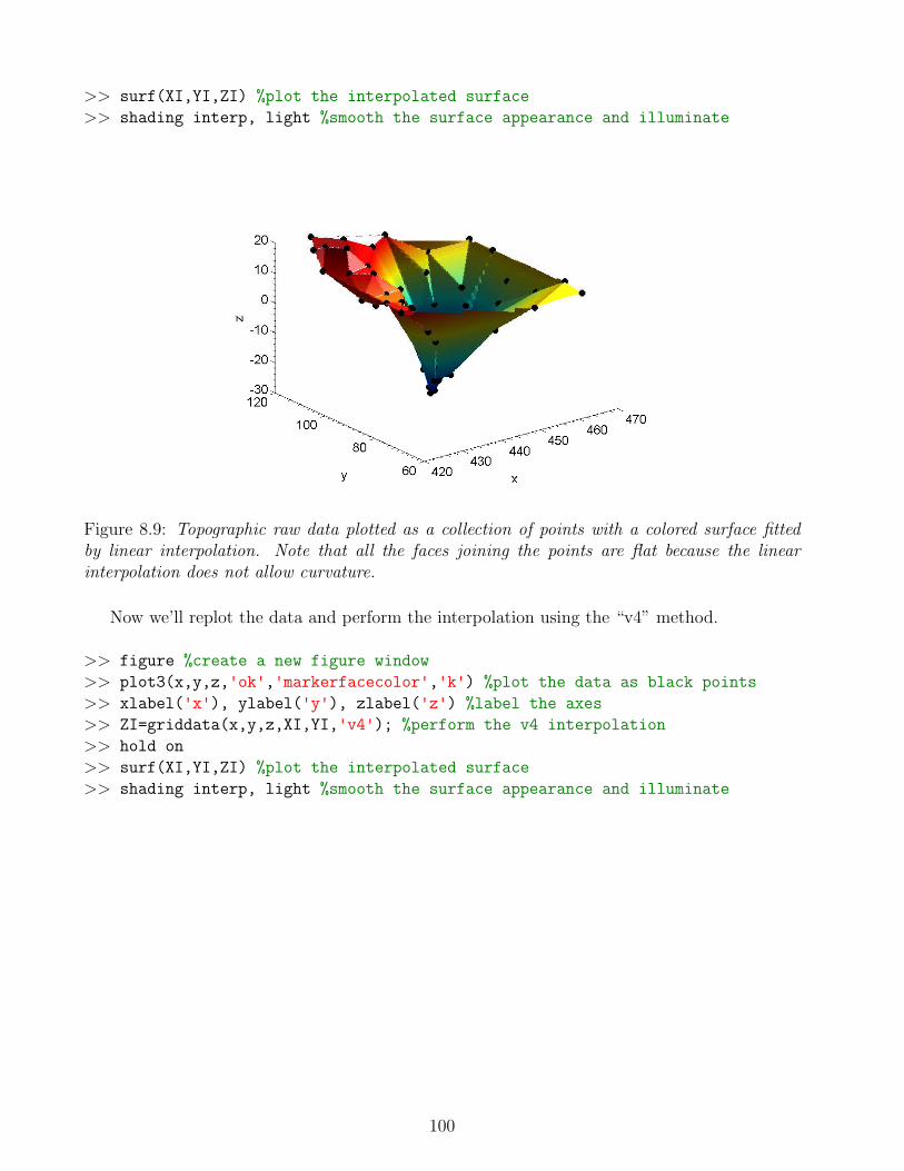
>> surf(XI,YI,ZI) %plot the interpolated surface
>> shading interp, light %smooth the surface appearance and illuminate
Figure 8.9: Topographic raw data plotted as a collection of points with a colored surface fittedby linear interpolation. Note that all the faces joining the points are flat because the linearinterpolation does not allow curvature.
Now we’ll replot the data and perform the interpolation using the “v4” method.
>> figure %create a new figure window
>> plot3(x,y,z,'ok','markerfacecolor','k') %plot the data as black points
>> xlabel('x'), ylabel('y'), zlabel('z') %label the axes
>> ZI=griddata(x,y,z,XI,YI,'v4'); %perform the v4 interpolation
>> hold on
>> surf(XI,YI,ZI) %plot the interpolated surface
>> shading interp, light %smooth the surface appearance and illuminate
100
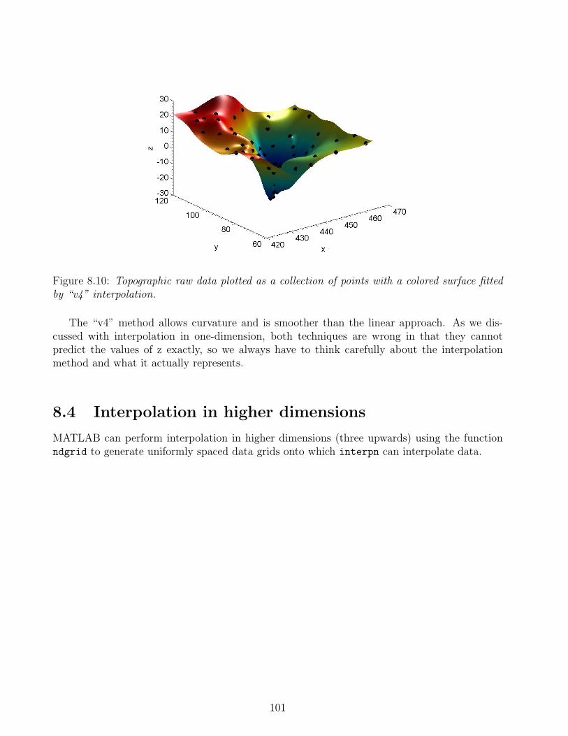
Figure 8.10: Topographic raw data plotted as a collection of points with a colored surface fittedby “v4” interpolation.
The “v4” method allows curvature and is smoother than the linear approach. As we dis-cussed with interpolation in one-dimension, both techniques are wrong in that they cannotpredict the values of z exactly, so we always have to think carefully about the interpolationmethod and what it actually represents.
8.4 Interpolation in higher dimensions
MATLAB can perform interpolation in higher dimensions (three upwards) using the functionndgrid to generate uniformly spaced data grids onto which interpn can interpolate data.
101

Chapter 9
Optimization
9.1 Minimization in one dimension
We are interested in finding the minimum value of the function:
f(x) =−1
(x− 0.3)2 + 0.01− 1
(x− 0.9)2 + 0.04− 6 (9.1)
If possible the best first step is to look how the function behaves over a range of different xvalues. To do this we must first write a MATLAB function to perform the calculation. This issimply:
function y=myfunction(x)
%Calculation of equation 9.1
y=-1./((x-0.3).∧2+0.01)-1./((x-0.9).∧2+0.04)-6;
Now we can calculate the value of equ. 9.1 for a series of x values.
>> x = linspace(-1,2,100); %100 equally spaced values between -1 and 2
>> y = myfunction(x); %call the function using the values in x
>> plot(x,y) %plot the result
>> xlabel('x') %add the x-axis label
>> ylabel('y') %add the y-axis label
Visual inspection shows us the the minimum is around x ∼ 0.3. But we can use MATLABto make a better evaluation, using the technique of minimization. The function fminsearch
will numerically find the minimum value of a provided function from a predefined starting point(in other words our first guess for the value of x ). The call to fminsearch is simple, you providethe name of the function you wish to minimize, the variable to use, and your starting point. In
102
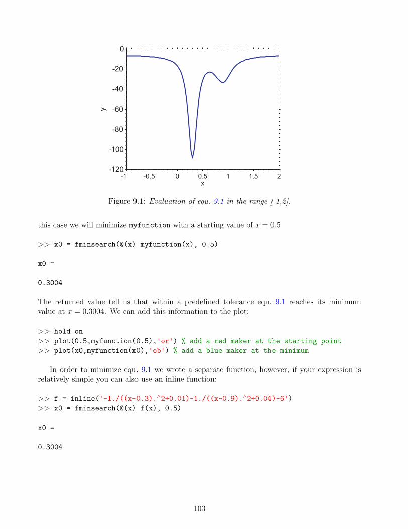
-1 -0.5 0 0.5 1 1.5 2-120
-100
-80
-60
-40
-20
0
x
y
Figure 9.1: Evaluation of equ. 9.1 in the range [-1,2].
this case we will minimize myfunction with a starting value of x = 0.5
>> x0 = fminsearch(@(x) myfunction(x), 0.5)
x0 =
0.3004
The returned value tell us that within a predefined tolerance equ. 9.1 reaches its minimumvalue at x = 0.3004. We can add this information to the plot:
>> hold on
>> plot(0.5,myfunction(0.5),'or') % add a red maker at the starting point
>> plot(x0,myfunction(x0),'ob') % add a blue maker at the minimum
In order to minimize equ. 9.1 we wrote a separate function, however, if your expression isrelatively simple you can also use an inline function:
>> f = inline('-1./((x-0.3).∧2+0.01)-1./((x-0.9).∧2+0.04)-6')
>> x0 = fminsearch(@(x) f(x), 0.5)
x0 =
0.3004
103

-1 -0.5 0 0.5 1 1.5 2-120
-100
-80
-60
-40
-20
0
x
y
Figure 9.2: Minimization of equ. 9.1, from the starting point x = 0.5. The starting point isshown as a red circle, the finishing point as a blue circle.
9.1.1 How does it work?
There are a wide variety of different methods with which to perform minimization, each ofwhich is suitable for different kinds or problems. One of the most commonly employed (and thesimplest to understand) techniques is the so-called “gradient descent” method. To understandthe ideas behind gradient descent we will use a zoom-up of our myfunction example. We canthink of the shape of our function defined in equ. 9.1 as a hilly topography, if we placed a ballat position, x = 0.5, the ball would roll down the hill until is stops in the deepest part of thevalley, which of course represents the minimum we are looking for.
104

0 0.2 0.4 0.6 0.8 1-120
-100
-80
-60
-40
-20
0
x
y
Figure 9.3: From its starting point at x = 0.5, the ball rolls down the hill until it stops in thedeepest part of the valley, which is our minimum at x = 0.3004
The fminsearch function performs this task iteratively from the provided starting point, ifincreasing x produces a decrease in y, then a small positive change is made to the estimate ofx. Alternatively, if decreasing x results in decreasing y then a small negative change is made toour estimate of x. In this way the algorithm follows the value of the function downhill, hencethe name “gradient descent”. This approach is simple but it does have its limitations, lets lookat what happens if we try to find the minimum of the function from a starting point of x = 1.3.
>> x0 = fminsearch(@(x) myfunction(x), 1.3)
x0 =
0.8927
We have obtained a different result! However if we look at the shape of the functionit is not difficult to see why this is the case. The gradient descent method will always move“downhill” so from our starting point at x = 1.3 it heads towards the small valley at x = 0.8927,but then gets stuck. Once at the bottom of this valley y is increasing when x is either increasedor decreased, so the algorithm would effectively have to travel “uphill” in order to reach theminimum at x = 0.3004, which is not allowed.
105
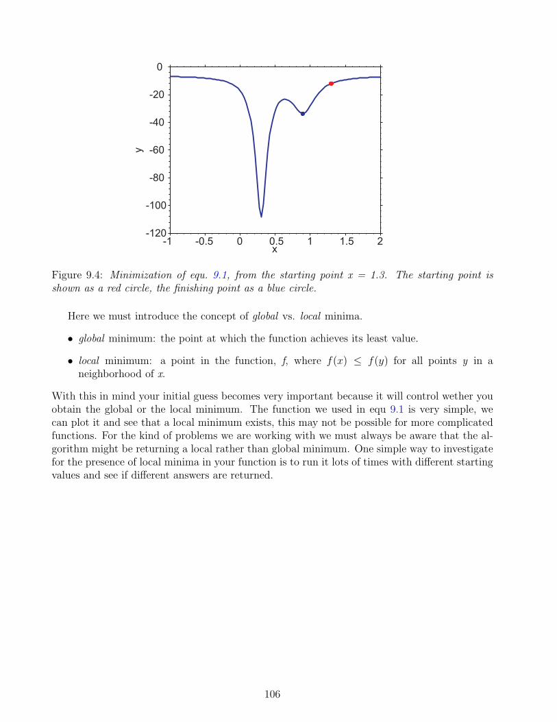
-1 -0.5 0 0.5 1 1.5 2-120
-100
-80
-60
-40
-20
0
x
y
Figure 9.4: Minimization of equ. 9.1, from the starting point x = 1.3. The starting point isshown as a red circle, the finishing point as a blue circle.
Here we must introduce the concept of global vs. local minima.
• global minimum: the point at which the function achieves its least value.
• local minimum: a point in the function, f, where f(x) ≤ f(y) for all points y in aneighborhood of x.
With this in mind your initial guess becomes very important because it will control wether youobtain the global or the local minimum. The function we used in equ 9.1 is very simple, wecan plot it and see that a local minimum exists, this may not be possible for more complicatedfunctions. For the kind of problems we are working with we must always be aware that the al-gorithm might be returning a local rather than global minimum. One simple way to investigatefor the presence of local minima in your function is to run it lots of times with different startingvalues and see if different answers are returned.
106
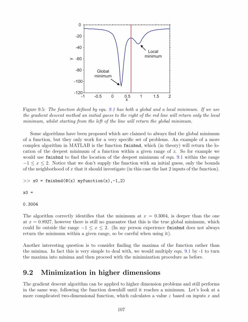
-1 -0.5 0 0.5 1 1.5 2-120
-100
-80
-60
-40
-20
0
x
yGlobal
minimum
Localminimum
Figure 9.5: The function defined by equ. 9.1 has both a global and a local minimum. If we usethe gradient descent method an initial guess to the right of the red line will return only the localminimum, whilst starting from the left of the line will return the global minimum.
Some algorithms have been proposed which are claimed to always find the global minimumof a function, but they only work for a very specific set of problems. An example of a morecomplex algorithm in MATLAB is the function fminbnd, which (in theory) will return the lo-cation of the deepest minimum of a function within a given range of x. So for example wewould use fminbnd to find the location of the deepest minimum of equ. 9.1 within the range−1 ≤ x ≤ 2. Notice that we don’t supply the function with an initial guess, only the boundsof the neighborhood of x that it should investigate (in this case the last 2 inputs of the function).
>> x0 = fminbnd(@(x) myfunction(x),-1,2)
x0 =
0.3004
The algorithm correctly identifies that the minimum at x = 0.3004, is deeper than the oneat x = 0.8927, however there is still no guarantee that this is the true global minimum, whichcould lie outside the range −1 ≤ x ≤ 2. (In my person experience fminbnd does not alwaysreturn the minimum within a given range, so be careful when using it).
Another interesting question is to consider finding the maxima of the function rather thanthe minima. In fact this is very simple to deal with, we would multiply equ. 9.1 by -1 to turnthe maxima into minima and then proceed with the minimization procedure as before.
9.2 Minimization in higher dimensions
The gradient descent algorithm can be applied to higher dimension problems and still performsin the same way, following the function downhill until it reaches a minimum. Let’s look at amore complicated two-dimensional function, which calculates a value z based on inputs x and
107

y.
z = f(x, y) =3(1− x)2 exp(−x2 − (y + 1)2)
− 1(x
5− x3 − y5
)exp(−x2 − y2)
− 1
3exp(−(x+ 1)2 − y2)
(9.2)
This is probably a bit too complicated to write as a single inline function, so again we will writea separate m-function file, but we have to take into account the manner in which fminsearch
works. The fminsearch function only allows one variable to be changed during the minimiza-tion, therefore we must input x and y together as a single variable. The easiest way to do thisis to combine x and y for the call to the function, but then split them once they are inside thefunction. Therefore we’ll use one input variable xy, the first column of which is the x data andthe second column of which is the y data.
function z=myfunction2(xy)
%function to calculate equ. 9.2
%to make things easier we’ll split the calculation into 3 parts
x=xy(:,1); y=xy(:,2) split the data into its x and y components
A=3.*(1-x).∧2.*exp(-x.∧2-(y+1).∧2);
B=-10.*(x./5-x.∧3-y.∧5).*exp(-x.∧2-y.∧2);
C=-1./3.*exp(-(x+1).∧2-y.∧2);
z = A + B + C;
First we should look at the shape of the function, to act as an input we need matrices rep-resenting x,y. To do this we can use the meshgrid function that we used previously:
>> [x,y]=meshgrid(-3:0.1:3,-3:0.1:3); %generate the (x,y) data
>> z = myfunction2([x(:),y(:)]); % combine x and y, and determine the value
>> surfc(x,y,z) %plot as a surface with contour lines
>> colormap gray %use the grayscale color map
>> xlabel('x') %add a label to the x-axis
>> ylabel('y') %add a label to the y-axis
>> zlabel('z') %add a label to the z-axis
108

−20
2
−2
0
2
−10
−5
0
5
10
xy
z
Figure 9.6: The two-dimensional function defined by equ. 9.2. Use the Rotate3D option toexamine the topography, you should see that there are three minima; two local and one global.
We can locate the minima in equ. 9.2 using fminsearch in the same manner as we did forthe one-dimensional case. The only difference is that because we are now working with x and ycoordinates we need to supply a first guess for each one (entered into function as a single array).Lets start with an initial guess of (1.1,-0.6):
>> hold on
>> xy0 = fminsearch(@(xy) myfunction2(xy),[1.1,-0.6])
>> plot3(1.1,-0.6,myfunction2([1.1 -0.6]),'or') %plot the starting point
>> plot3(xy0(1),xy0(2),myfunction2(xy0),'ob') %plot the finishing point
−3 −2 −1 0 1 2 3−2
0
2
−10
−5
0
5
10
xy
z
Figure 9.7: Minimization of equ. 9.2, using fminsearch from a starting point of (1.1,-0.6). Thestarting point is shown as a red circle, the finishing point as a green circle.
As with the one-dimensional case, fminsearch will work downhill towards a minimum, whichmay not necessarily be the global minimum.
109
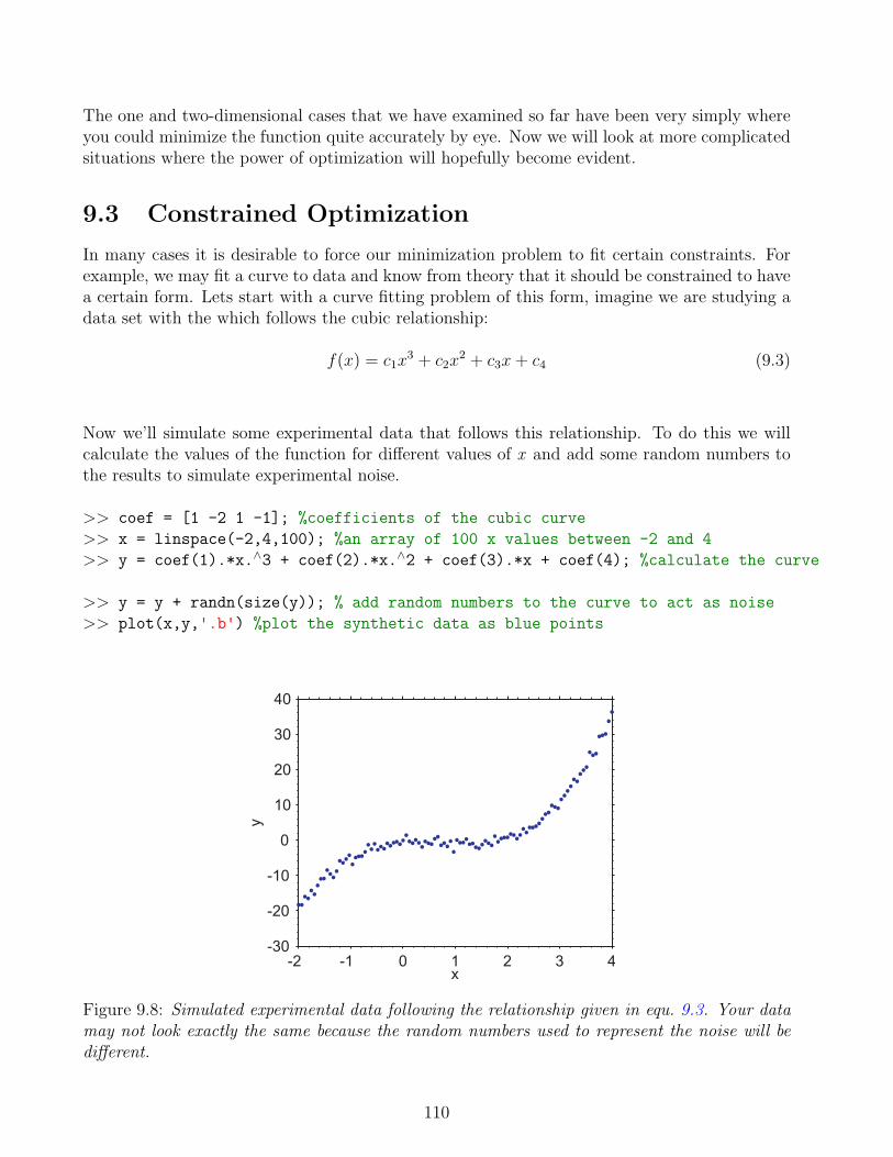
The one and two-dimensional cases that we have examined so far have been very simply whereyou could minimize the function quite accurately by eye. Now we will look at more complicatedsituations where the power of optimization will hopefully become evident.
9.3 Constrained Optimization
In many cases it is desirable to force our minimization problem to fit certain constraints. Forexample, we may fit a curve to data and know from theory that it should be constrained to havea certain form. Lets start with a curve fitting problem of this form, imagine we are studying adata set with the which follows the cubic relationship:
f(x) = c1x3 + c2x
2 + c3x+ c4 (9.3)
Now we’ll simulate some experimental data that follows this relationship. To do this we willcalculate the values of the function for different values of x and add some random numbers tothe results to simulate experimental noise.
>> coef = [1 -2 1 -1]; %coefficients of the cubic curve
>> x = linspace(-2,4,100); %an array of 100 x values between -2 and 4
>> y = coef(1).*x.∧3 + coef(2).*x.∧2 + coef(3).*x + coef(4); %calculate the curve
>> y = y + randn(size(y)); % add random numbers to the curve to act as noise
>> plot(x,y,'.b') %plot the synthetic data as blue points
-2 -1 0 1 2 3 4-30
-20
-10
0
10
20
30
40
x
y
Figure 9.8: Simulated experimental data following the relationship given in equ. 9.3. Your datamay not look exactly the same because the random numbers used to represent the noise will bedifferent.
110

We can use minimize the “sum of squared residuals” to find the best fit to the data. In thiscase we will fit a cubic polynomial to the data, but of course we won’t get a perfect fit becausewe have added a noise component. First we need to calculate the value of the line for a givenset of coefficients (which we will store in the vector, c) and then determine the difference to thedata, i.e. determine the residuals.
function ssr = objfun(c,xdata,ydata)
%objective function to calculate residuals on a cubic fit
%calculate the line given the coefficients in c
yhat=c(1).*xdata.∧3 + c(2).*xdata.∧2 + c(3).*xdata + c(4);
%calculate the sum of the squared residuals by comparing to ydata
ssr = sum((ydata-yhat).∧2);
The optimal fit to the data is found when we minimize the sum of the squared residuals.We can do this using fminsearch, with a starting guess of c of all zeros. When we have theoptimized version of c we can calculate and plot the best fit line for our different values of x.
>> c = fminsearch(@(c) objfun(c,x,y),[0 0 0 0]) %minimize the residuals
>> y0 = c(1).*x.∧3 + c(2).*x.∧2 + c(3).*x + c(4); %the fitted cubic curve
>> hold on
>> plot(x,y0,'r','linewidth',1) %plot the fitted curve as a red line
-2 -1 0 1 2 3 4-30
-20
-10
0
10
20
30
40
x
y
Figure 9.9: Optimized cubic fit (red line) to the experimental data (blue dots).
The fit seems to be okay, but imagine the situation where theory tells us the fitted curve hasto obey certain constraints. The function fminsearch can only perform unconstrained mini-mization, so instead we must use the function fmincon, which has addition inputs which allowyou to add problem constraints. The inputs are quite complex, but they allow us to definelinear inequalities, linear equalities and bounds; they are as follows:
111

c = fmincon(function,c0,A,b,Aeq,beq,lb,ub)
minimize f(c) such that:
A · c ≤ b
Aeq · c = beq
lb ≤ c ≤ ub
(9.4)
So what does all of this mean? The constraints allow us to find a solution to the minimizationproblem which meet certain requirements. Lets look at the statements one by one, in all casesthe final solution of the minimization is represented by c:
• A · c ≤ b, we can define a set of values in A that when matrix multiplied by c must be lessthan or equal to the defined value b.
• Aeq · c ≤ beq, we can define a set of values in A that when matrix multiplied by c mustbe equal to the defined value b.
• lb ≤ c ≤ ub, all the values in c must be greater than or equal to the lower bound, lb, andless than or equal to the upper bound, ub.
9.3.1 Linear Equalities
We’ll start by enforcing a constraint that the curve must pass through the point (-2,-19). Todo this we must use the linear equalities option, which can be written in the form:
A = [−23,−22,−2, 1]
A · c = −19
In MATLAB notation we can set the constraints and call the function in the following way:
>> xc = -2 %define the constrained x value
>> yc = -19 %define the constrained y value
>> Aeq=xc.∧[3,2,1,0]; %left-hand side of the constraint
>> beq=yc; %right-hand side of the constraint
>> c=fmincon(@(c) objfun(c,x,y),[0 0 0 0],[],[],Aeq,beq,[],[]); %call fmincon
>> y0 = c(1).*x.∧3 + c(2).*x.∧2 + c(3).*x + c(4); %the fitted cubic curve
>> plot(x,y0,'k','linewidth',1) %plot the fitted curve as a black line
112

-2 -1 0 1 2 3 4-30
-20
-10
0
10
20
30
40
x
y
Figure 9.10: Optimized cubic fit (black line) to the experimental data (blue dots) constrained topass through the point (-2,-19).
We can look at the returned coefficients in c, and check that Aeq · c does in fact equal beq.
>> c'%display the coefficients as a column
ans =
1.0281
-2.0414
0.8203
-0.9689
>> Aeq*c'%check the equality constraint
ans =
-19
To add more equality constraints is simple, we just need to combine them into a matrix withone for each constraint. We have our first constraint that the fitted line must pass through thepoint (-2,-19), now lets add another constraint to also force the line through (0,-1):
>> Aeq(1,:)=(-2).∧[3,2,1,0]; %left-hand side of the 1st constraint
>> beq(1,1)=-19; %right-hand side of the 1st constraint
>> Aeq(2,:)=0.∧[3,2,1,0]; %left-hand side of the 2nd constraint
>> beq(2,1)=-1; %right-hand side of the 2nd constraint
>> c=fmincon(@(c) objfun(c,x,y),[0 0 0 0],[],[],Aeq,beq,[],[]); %call fmincon
>> y2 = c(1).*x.∧3 + c(2).*x.∧2 + c(3).*x + c(4); %the fitted cubic curve
>> plot(x,y2,'g','linewidth',1) %plot the fitted curve as a green line
>> Aeq*c'%check the inequality constraint
ans =
113
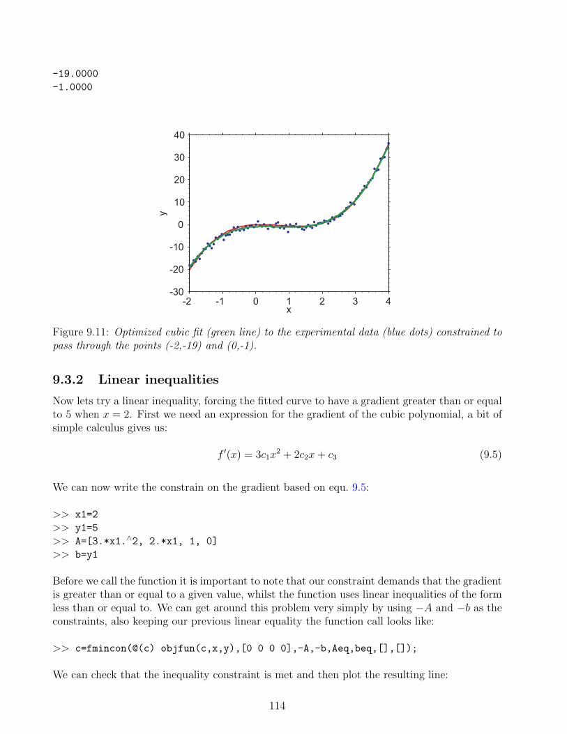
-19.0000
-1.0000
-2 -1 0 1 2 3 4-30
-20
-10
0
10
20
30
40
x
y
Figure 9.11: Optimized cubic fit (green line) to the experimental data (blue dots) constrained topass through the points (-2,-19) and (0,-1).
9.3.2 Linear inequalities
Now lets try a linear inequality, forcing the fitted curve to have a gradient greater than or equalto 5 when x = 2. First we need an expression for the gradient of the cubic polynomial, a bit ofsimple calculus gives us:
f ′(x) = 3c1x2 + 2c2x+ c3 (9.5)
We can now write the constrain on the gradient based on equ. 9.5:
>> x1=2
>> y1=5
>> A=[3.*x1.∧2, 2.*x1, 1, 0]
>> b=y1
Before we call the function it is important to note that our constraint demands that the gradientis greater than or equal to a given value, whilst the function uses linear inequalities of the formless than or equal to. We can get around this problem very simply by using −A and −b as theconstraints, also keeping our previous linear equality the function call looks like:
>> c=fmincon(@(c) objfun(c,x,y),[0 0 0 0],-A,-b,Aeq,beq,[],[]);
We can check that the inequality constraint is met and then plot the resulting line:
114
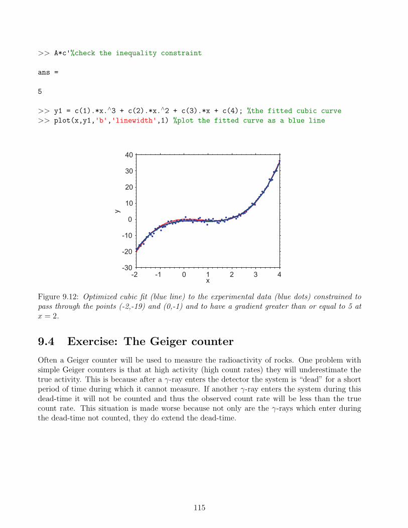
>> A*c'%check the inequality constraint
ans =
5
>> y1 = c(1).*x.∧3 + c(2).*x.∧2 + c(3).*x + c(4); %the fitted cubic curve
>> plot(x,y1,'b','linewidth',1) %plot the fitted curve as a blue line
-2 -1 0 1 2 3 4-30
-20
-10
0
10
20
30
40
x
y
Figure 9.12: Optimized cubic fit (blue line) to the experimental data (blue dots) constrained topass through the points (-2,-19) and (0,-1) and to have a gradient greater than or equal to 5 atx = 2.
9.4 Exercise: The Geiger counter
Often a Geiger counter will be used to measure the radioactivity of rocks. One problem withsimple Geiger counters is that at high activity (high count rates) they will underestimate thetrue activity. This is because after a γ-ray enters the detector the system is “dead” for a shortperiod of time during which it cannot measure. If another γ-ray enters the system during thisdead-time it will not be counted and thus the observed count rate will be less than the truecount rate. This situation is made worse because not only are the γ-rays which enter duringthe dead-time not counted, they do extend the dead-time.
115

Figure 9.13: How can we find the true count rate of a Geiger counter which suffers from dead-time.
The relationship between the observed count rate (Nobs) and the true count rate (Ntrue) isan exponential law equation:
Nobs = Ntruee−Ntrueτ
where τ is the dead-time per pulse (20 x 10−6 seconds in old instruments). Note this is a tran-scendental equation which means that it cannot be rewritten in the form Ntrue = .... In thisexercise you will use fminsearch to determine the value of Ntrue when Nobs = 8000 cps and τ= 20 x 10−6 s.
Steps to completing the exercise
Don’t forget that we have examined this problem before when we discussed writingfunctions. In the previous case we found our best estimate by finding the value ofNtrue which produced the minimum squared difference of the count rate equation withthe observed count rate.
• Find an expression which you can minimize to find the best estimate of Ntrue.
• Write this expression as an inline function.
• Minimize the function using fminsearch and an initial guess of Ntrue.
Functions you may find useful
• exp - Exponential.
• inline - Construct INLINE object.
• fminsearch - Multidimensional unconstrained nonlinear minimization.
116

Chapter 10
Final Project
10.1 Sand, Silt and Clay in an Arctic Lake
As a final project we are going to plot and analyze some grain size composition data from alake in the Arctic. This will require you to undertake all stages of the analysis process fromimporting your data to plotting your final results. There are a number of steps involved anddon’t be surprised if this takes some time.
10.1.1 Importing the data
The lake grain size data is stored in the EXCEL file lakegrainsize.xls, import the data intoMATLAB in a form that you can work with it.
10.1.2 Plotting the data
Plot the grain size data in a ternary plot (look on the MathWorks File-exchange to find functionswhich will produce ternary plots, or if your feeling confident write your own function). Yourfinal graphic could look something like the following figure.
117
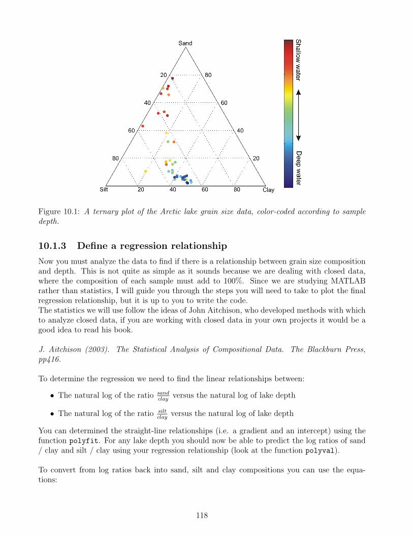
Figure 10.1: A ternary plot of the Arctic lake grain size data, color-coded according to sampledepth.
10.1.3 Define a regression relationship
Now you must analyze the data to find if there is a relationship between grain size compositionand depth. This is not quite as simple as it sounds because we are dealing with closed data,where the composition of each sample must add to 100%. Since we are studying MATLABrather than statistics, I will guide you through the steps you will need to take to plot the finalregression relationship, but it is up to you to write the code.The statistics we will use follow the ideas of John Aitchison, who developed methods with whichto analyze closed data, if you are working with closed data in your own projects it would be agood idea to read his book.
J. Aitchison (2003). The Statistical Analysis of Compositional Data. The Blackburn Press,pp416.
To determine the regression we need to find the linear relationships between:
• The natural log of the ratio sandclay
versus the natural log of lake depth
• The natural log of the ratio siltclay
versus the natural log of lake depth
You can determined the straight-line relationships (i.e. a gradient and an intercept) using thefunction polyfit. For any lake depth you should now be able to predict the log ratios of sand/ clay and silt / clay using your regression relationship (look at the function polyval).
To convert from log ratios back into sand, silt and clay compositions you can use the equa-tions:
118

sand =elog( sand
clay)
elog( sandclay
) + elog( siltclay
) + 1
silt =elog( silt
clay)
elog( sandclay
) + elog( siltclay
) + 1
clay =1
elog( sandclay
) + elog( siltclay
) + 1
10.1.4 Plot the regression relationship
Plot the regression line predicting grain size composition for a series of depths through the lake.Your final result should look something like the graphic below.
Figure 10.2: A ternary plot of the Arctic lake grain size data color-coded according to sampledepth. The black line shows the regression relationship, the dashes indicate where extrapolationwas necessary.
119

Steps to completing the exercise
As a review of the material above the basic steps to complete the exercise are as follows:
• Import the data from Lakegrainsize.xls and give the variables appropriate names.
• Plot the data in a ternary plot.
• Find the straight-line relationships between the log of depth and the log-ratiosof the grain sizes.
• Create an array of depth values.
• Find the log-ratios of the grain sizes for the new log depths according to thestraight-line relationships.
• Convert the log-ratio grain sizes back into sand, silt and clay proportions.
• Add the sand, silt and clay proportions from the regression into the ternary plot.
Functions you may find useful
• xlsread - Read Microsoft Excel spreadsheet file.
• ternplot - Plot ternary phase diagram (available from The Mathworks file-exchange).
• ternlabel - label ternary phase diagram (available from The Mathworks file-exchange).
• log - Natural logarithm.
• exp - Exponential.
• polyfit - Polynomial curve fitting.
• polyval - Polynomial evaluation.
10.2 Exercise: Bringing it all together with cars and
goats
If you still have some time left over you can try this final exercise, it is fun but challenging,some of you might be familiar with the problem because it is quite famous. Again you shouldthink about how to work a solution to the problem before thinking about how specifically toperform the task in MATLAB. This problem is known as the “Monty Hall” problem and was
120

brought to fame when discussed by the world’s “most intelligent” person Marilyn vos Savant(she has a quoted IQ of 228). The statement of the problem is as follows:
Suppose you’re on a game show, and you’re given the choice of three doors: Behind one door isa car; behind the others, goats. You pick a door, say A, and the host, who knows what’s behindthe doors, opens another door, say C, which has a goat. He then says to you, “Do you want topick door B?” Is it to your advantage to switch your choice?
Figure 10.3: In search of a new car, the player picks a door, say A. The game host then opensone of the other doors, say C, to reveal a goat and offers to let the player pick door B insteadof door A.
.
At first glance it appears the problem comes down to a 50:50 choice and therefore froma probability point of view there is no advantage or disadvantage to switching your choice orsticking with your original choice. However, if you work through the probabilites properly youfind that the chances of winning a car are twice as high if you switch compared to sticking withyou original choice. This does indeed seem to be a counterintuitive result so we’ll attempt towrite a MATLAB script which simulates the game. The game can then be run 1 million times(you need a for loop to do this) with the various possibilities being played out (you can userelational and logical operators to do this). Does you numerical model get close the result fromprobability theory? If you are new to programming and MATLAB you may find this exercisevery challenging, so don’t feel too depressed if you can’t complete it.
121

Steps to completing the exercise
This exercise can be solved with a few inbuilt functions (the list below might give yousome clues on how to proceed). To solve the problem take the following steps
• Think.
• Think some more.
• Find the solution.
Functions you may find useful
• rand - Uniformly distributed pseudo-random numbers.
• sort - Sort in ascending or descending order.
122

Chapter 11
Exercise Solutions
It is important to realize that the exercises in this course can be solved in a variety of differentways, therefore the solutions I will give are by no means the “definitive answer”. I’ve haveattempted to provide solutions which are written in a clear manner in order to help you under-stand what is happening, this means that the code may be somewhat inefficient and from thepoint of view of computation speed can certainly be improved.
11.1 Solution: Mmmm, π
There are three main tasks to solve this exercise:
1. Generating the numbers between 0 and 10000 to act as n.
2. Calculating the terms of the series using the values of n.
3. Finally, summing the series and multiplying by 4 to estimate π.
These three tasks can be performed using simple one-line commands. First we need to generatea variable n which contains the integers between 0 and 10000:
>> n = [0:1:10000];
Now we must calculate each term of the series according to expression:
(−1)n
2n+ 1
We’ll perform this calculation and place the result in a variable called terms (note, my variablenames are completely arbitrary, you can use any names you want as long as they follow therules we discussed earlier).
>> terms = (-1).^n./(2*n+1);
You’ll notice that the order of evaluation is important here and it is necessary to place bracketsaround the -1. Finally, we simply need to add all the terms together using the inbuilt sum
function and multiply by 4 to make our estimate of π.
123

>> p = sum(terms)*4
Putting this all together our script for estimating π using the method of Madhava of Sangam-agrama would look like:
n = [0:1:10000];
terms = (-1).^n./(2*n+1);
p = sum(terms)*4
11.1.1 Golf Solution: Mmmm, π
If you remember, MATLAB Golf involves coding a problem in as few characters as possible.The following lines present one solution in a compact form which takes advantage of a numberof MATLAB’s shortcuts. It uses 30 characters:
>> n=0:1e4
>> sum((-1).^n./(2*n+1))*4
11.2 Solution: Mmmm, a second helping of π
To convert our script file into M-function we need to perform three tasks:
1. Add a header line defining the function name (madhava), the input (N) and output (p).
2. Define the values of n to be used as ranging between 0 and N
3. Add suitable help and comments
Our original script file looked like:
n = [0:1:10000];
terms = (-1).^n./(2*n+1);
p = sum(terms)*4
In order to convert this into a M-function we just add an appropriate header line and giveN as the maximum value of n.
function p = madhava(N)
n = [0:1:N];
terms = (-1).^n./(2*n+1);
p = sum(terms)*4;
124

Once the function is saved (make sure the filename is the same as the defined function name)you can call it from the MATLAB command window with a defined value of N.
>> p = madhava(10000)
p =
3.1417
We should also add help and comments to explain the purpose of the function and the steps itmakes in the calculation.
function p = madhava(N)
%madhava - Estimate pi using the Madhava-Leibniz series
%
% Syntax: p = madhava(N)
%
% Inputs:
% N - the maximum term to be included
%
% Outputs:
% p - estimate of pi
%
% Other m-files required: none
% Subfunctions: none
% MAT-files required: none
%
% Author: Dave Heslop
% Department of Geosciences, University of Bremen
% email address: [email protected]
% Last revision: 6-Dec-2008
%------------- BEGIN CODE --------------
n = [0:1:N]; %form the integer terms
terms = (-1).^n./(2*n+1); %calculate series terms
p = sum(terms)*4; %sum all terms (to give pi/4) and multiply
%------------- END CODE --------------
11.3 Solution: The Geiger counter
This exercise is more complicated than the previous ones. We will solve it in a simple way bytesting a number of possible values of Ntrue then selecting the one which gives a value closestto our desired Nobs. We’ll start by developing the code in a script file with fixed values of
125

Nobs = 8000 cps and τ = 20 x 10−6 s. The first thing to do is define these values in suitablynamed variables:
>> Nobs=8000;
>> tau=20e-6;
Now we’ll create an array of Ntrue values to test, in this case ranging between 1 and 100000:
>> Ntest=[1:1e5];
To calculate the observed count rate which would be produced by each of the values in Ntest
we place them in our equation:
>> Ncalc=Ntest.*exp(-Ntest.*tau);
We now have an array (Ncalc) which contains the predicted observed count rate for each of theguessed values in Ntest. To find which produces a prediction which is closest to Nobs we takethe root squared difference between Ncalc and Nobs:
>> Ndiff=sqrt((Ncalc-Nobs).^2);
The position within Ndiff that has the smallest value tells us the location in Ntest whichprovides the best prediction for Nobs. To find this index position we can use the inbuilt func-tion sort, this takes an array and reorders it from lowest to highest value and gives a secondoutput with the original index positions of the values before they were sorted.
>> [Ndiff min,idx]=sort(Ndiff);
We now know that our best guess for Ntrue lies in Ntest at the index given in the first po-sition of idx:
>> Ntrue=Ntest(idx(1))
Ntrue =
9716
So, for an observed count rate of 8000 cps and τ = 20 x 10−6 s, we can estimate that Ntrue
= 9716 cps. We now have the basic workings of our code and we need to convert it into anM-function. This means we need to think about input and output values. The required inputswill be:
• The observed count rate (called Nobs)
• The dead-time (called tau)
• The array of values to test (called Ntest)
126
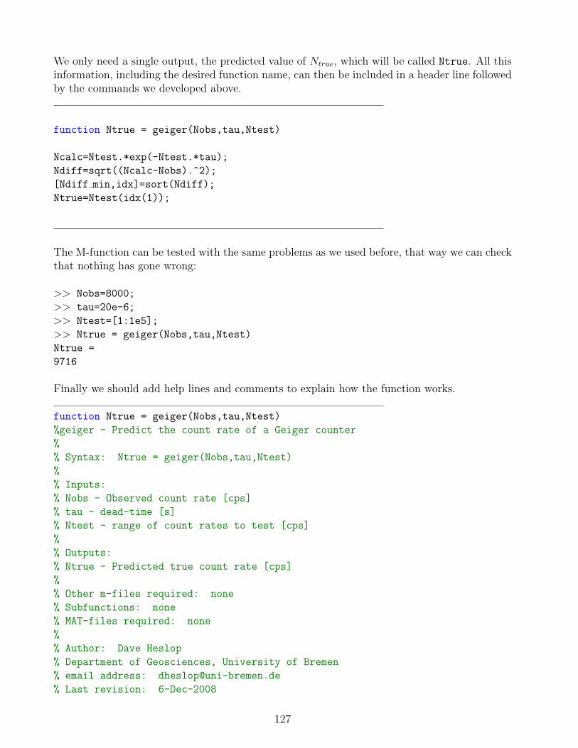
We only need a single output, the predicted value of Ntrue, which will be called Ntrue. All thisinformation, including the desired function name, can then be included in a header line followedby the commands we developed above.
function Ntrue = geiger(Nobs,tau,Ntest)
Ncalc=Ntest.*exp(-Ntest.*tau);
Ndiff=sqrt((Ncalc-Nobs).^2);
[Ndiff min,idx]=sort(Ndiff);
Ntrue=Ntest(idx(1));
The M-function can be tested with the same problems as we used before, that way we can checkthat nothing has gone wrong:
>> Nobs=8000;
>> tau=20e-6;
>> Ntest=[1:1e5];
>> Ntrue = geiger(Nobs,tau,Ntest)
Ntrue =
9716
Finally we should add help lines and comments to explain how the function works.
function Ntrue = geiger(Nobs,tau,Ntest)
%geiger - Predict the count rate of a Geiger counter
%
% Syntax: Ntrue = geiger(Nobs,tau,Ntest)
%
% Inputs:
% Nobs - Observed count rate [cps]
% tau - dead-time [s]
% Ntest - range of count rates to test [cps]
%
% Outputs:
% Ntrue - Predicted true count rate [cps]
%
% Other m-files required: none
% Subfunctions: none
% MAT-files required: none
%
% Author: Dave Heslop
% Department of Geosciences, University of Bremen
% email address: [email protected]
% Last revision: 6-Dec-2008
127

%------------- BEGIN CODE --------------
Ncalc=Ntest.*exp(-Ntest.*tau); %predicted cps
Ndiff=sqrt((Ncalc-Nobs).^2); %rs difference with observed
[Ndiff min,idx]=sort(Ndiff); %locate smallest difference
Ntrue=Ntest(idx(1)); %select best fitting value
%------------- END CODE --------------
11.4 Solution: Classifying sediments
In this exercise you were asked to analyze grain size data from the file grainsize.mat in order tofind how many samples contained certain amounts of sand, silt and clay. Specifically:
1. How many samples contain more than 50% sand?
2. How many samples contain more than 50% silt?
3. How many samples contain more than 30% silt or more than 25% clay?
4. How many samples contain more than 40% sand, less than 40% silt and more than 40%clay?
The first task is to load the data into MATLAB (plus we will clear the memory before starting:
clear all
load grainsize
The variable gs is now in the memory which contains the data for the sand (first column),silt (second column) and clay (third column) percentages. Each row of the gs matrix representsa different sample. We now need to use a combination of relational and logical operators toanswer the questions. Lets start with “How many samples contain more than 50% sand?”. Thefirst thing we need to consider is that the information on sand content is contained in the firstcolumn of gs, therefore to access the sand content for all the samples we will use the addressgs(:,1). We can now find the number of samples with more than 50% sand in two differentways, in the first we will return an array of logical values (1s signify samples which meet thecriteria and 0s signify those that don’t) and simply add together all the entries:
>> output=gs(:,1)>50>> sum(output)
ans =
19
Alternatively, we can use the find function to provide an array containing the indices of thesamples which met the criteria and then simply find how many entries are in the array usingthe function numel:
128

>> idx=find(gs(:,1)>50)>> numel(idx)
ans =
19
For the remaining questions we will determine an array of logical values and sum the entriestogether in a single line. Notice how the addressing of the gs matrix changes in order to selectthe sand, silt and clay components as required and the inclusion of logical operators are com-binations of criteria have to be tested.
“How many samples contain more than 50% silt?”
>> sum(gs(:,2)>50)ans =
20
“How many samples contain more than 30% silt or more than 25% clay?”
>> sum(gs(:,2)>30 | gs(:,3)>25)ans =
90
“How many samples contain more than 40% sand, less than 40% silt and more than 40% clay?”
>> sum(gs(:,1)>40 & gs(:,3)<40 & gs(:,3)>40)ans =
0
11.5 Solution: The Safe Cracker
The solution to this exercise is a M-function which requires the following basic parts:
1. A name, we’ll use safe crack
2. Three inputs, the guessed digits of the combination which we will call A, B and C
3. Testing the combination and sending reports to the screen.
4. An output that we’ll call status which tells us the state of the safe (1 corresponds toopen, 0 to closed).
Therefore the header line of our M-function will look like:
function status=safe crack(A,B,C)
129
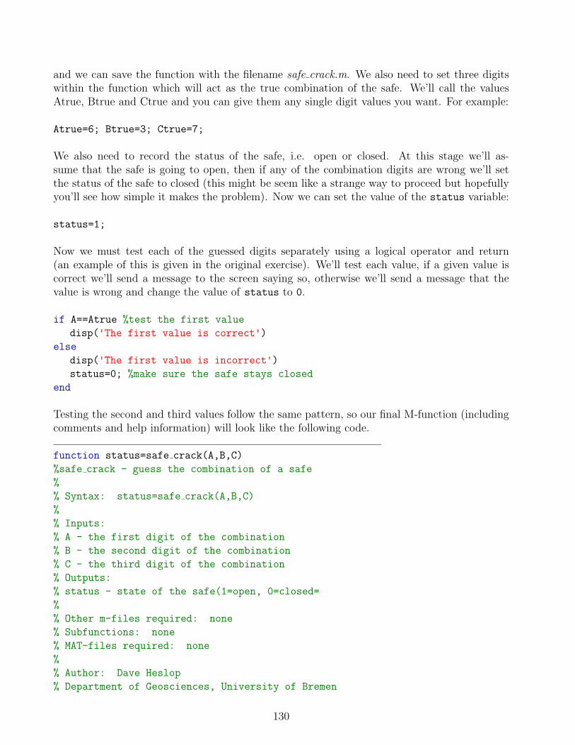
and we can save the function with the filename safe crack.m. We also need to set three digitswithin the function which will act as the true combination of the safe. We’ll call the valuesAtrue, Btrue and Ctrue and you can give them any single digit values you want. For example:
Atrue=6; Btrue=3; Ctrue=7;
We also need to record the status of the safe, i.e. open or closed. At this stage we’ll as-sume that the safe is going to open, then if any of the combination digits are wrong we’ll setthe status of the safe to closed (this might be seem like a strange way to proceed but hopefullyyou’ll see how simple it makes the problem). Now we can set the value of the status variable:
status=1;
Now we must test each of the guessed digits separately using a logical operator and return(an example of this is given in the original exercise). We’ll test each value, if a given value iscorrect we’ll send a message to the screen saying so, otherwise we’ll send a message that thevalue is wrong and change the value of status to 0.
if A==Atrue %test the first value
disp('The first value is correct')
else
disp('The first value is incorrect')
status=0; %make sure the safe stays closed
end
Testing the second and third values follow the same pattern, so our final M-function (includingcomments and help information) will look like the following code.
function status=safe crack(A,B,C)
%safe crack - guess the combination of a safe
%
% Syntax: status=safe crack(A,B,C)
%
% Inputs:
% A - the first digit of the combination
% B - the second digit of the combination
% C - the third digit of the combination
% Outputs:
% status - state of the safe(1=open, 0=closed=
%
% Other m-files required: none
% Subfunctions: none
% MAT-files required: none
%
% Author: Dave Heslop
% Department of Geosciences, University of Bremen
130

% email address: [email protected]
% Last revision: 6-Dec-2008
%------------- BEGIN CODE --------------%
Atrue=6; Btrue=3; Ctrue=7; % set the combination
status=1; %assume the safe will open
if A==Atrue %test the first value
disp('The first value is correct')
else
disp('The first value is incorrect')
status=0; %make sure the safe stays closed
end
if B==Btrue %test the first value
disp('The second value is correct')
else
disp('The second value is incorrect')
status=0; %make sure the safe stays closed
end
if C==Ctrue %test the first value
disp('The third value is correct')
else
disp('The third value is incorrect')
status=0; %make sure the safe stays closed
end
%------------- END CODE --------------%
11.6 Solution: An even worse safe
The extension to the previous function to test if the guessed digit is within ±1 of the true digitis simple and we’ll save the new function with the name safe crack2.m. Before we tested if theguessed digit was equal to the true digit with the == operator, for the new test we need tocheck the guess is both greater than or equal to the true digit minus 1 and less than or equalto the true digit plus 1. In the case of the first digit A we can do this with the relational andlogical operators:
A>=Atrue-1 & A<=Atrue+1
This means our final function with modifications for each of the three digits will look like:
function status=safe crack2(A,B,C)
131

%safe crack - guess the combination of a safe within -1 or +1
%
% Syntax: status=safe crack(A,B,C)
%
% Inputs:
% A - the first digit of the combination
% B - the second digit of the combination
% C - the third digit of the combination
% Outputs:
% status - state of the safe(1=open, 0=closed=
%
% Other m-files required: none
% Subfunctions: none
% MAT-files required: none
%
% Author: Dave Heslop
% Department of Geosciences, University of Bremen
% email address: [email protected]
% Last revision: 6-Dec-2008
%------------- BEGIN CODE --------------%
Atrue=6; Btrue=3; Ctrue=7; % set the combination
status=1; %assume the safe will open
if A>=Atrue-1 & A<=Atrue+1 %test the first value
disp('The first value is correct')
else
disp('The first value is incorrect')
status=0; %make sure the safe stays closed
end
if B>=Btrue-1 & B<=Btrue+1 %test the first value
disp('The second value is correct')
else
disp('The second value is incorrect')
status=0; %make sure the safe stays closed
end
if C>=Ctrue-1 & C<=Ctrue+1 %test the first value
disp('The third value is correct')
else
disp('The third value is incorrect')
status=0; %make sure the safe stays closed
end
%------------- END CODE --------------%
132

11.7 Solution: Life’s ups and downs in the Logistic Map
This exercise may appear to be more difficult that it actually is. As discussed in the exercisethe simplest approach is to write code for a single realization of r and xinitial and then extendit to consider multiple cases. For the single case we first need to generate a random value ofxinitial between 0 and 1 and r between 0 and 4. To do this we can use the rand function whichgives uniformly distributed random numbers in the range 0–1:
x=rand(1);
r=rand(1)*4;
Once we have these starting values we can employ a loop to iterate the logistic equation atotal of 2000 times, each time updating the existing value of x.
for i=1:2000
x=r.*x*(1-x);
end
The value of x will now represent xfinal for our specific case of r and xinitial. To extend thiscode to a large number of realizations so that we can plot the logistic map we need to generate alarge number of values of r and xinitial (in this example we’ll use 10000). Then we loop througheach realization, iterating the logistic equation 2000 times to produce all the values of xinitial.You’ll see that to iterate the equation for all the different cases we need to use two loops insideeach other:
N=1e4 %total number of realizations
x=rand(N,1); %generate the initial populations
r=rand(N,1)*4; %generate the values of r
for j=1:N %loop through all the realizations
for i=1:2000 %iterate the logistic equation
x(j)=r(j).*x(j)*(1-x(j)); %update the population
end
end
Finally we just need to plot the data and label the axes:plot(r,x,'.')
ylabel('x {final}')xlabel('r')
133
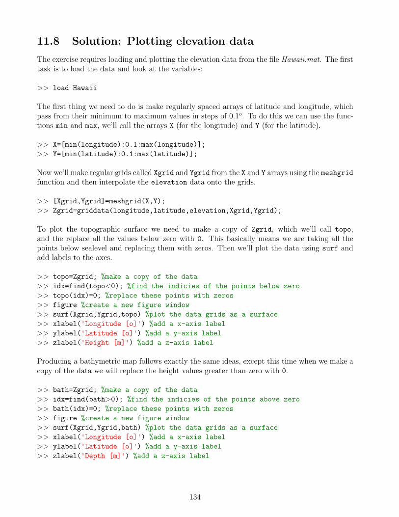
11.8 Solution: Plotting elevation data
The exercise requires loading and plotting the elevation data from the file Hawaii.mat. The firsttask is to load the data and look at the variables:
>> load Hawaii
The first thing we need to do is make regularly spaced arrays of latitude and longitude, whichpass from their minimum to maximum values in steps of 0.1o. To do this we can use the func-tions min and max, we’ll call the arrays X (for the longitude) and Y (for the latitude).
>> X=[min(longitude):0.1:max(longitude)];
>> Y=[min(latitude):0.1:max(latitude)];
Now we’ll make regular grids called Xgrid and Ygrid from the X and Y arrays using the meshgridfunction and then interpolate the elevation data onto the grids.
>> [Xgrid,Ygrid]=meshgrid(X,Y);
>> Zgrid=griddata(longitude,latitude,elevation,Xgrid,Ygrid);
To plot the topographic surface we need to make a copy of Zgrid, which we’ll call topo,and the replace all the values below zero with 0. This basically means we are taking all thepoints below sealevel and replacing them with zeros. Then we’ll plot the data using surf andadd labels to the axes.
>> topo=Zgrid; %make a copy of the data
>> idx=find(topo<0); %find the indicies of the points below zero
>> topo(idx)=0; %replace these points with zeros
>> figure %create a new figure window
>> surf(Xgrid,Ygrid,topo) %plot the data grids as a surface
>> xlabel('Longitude [o]') %add a x-axis label
>> ylabel('Latitude [o]') %add a y-axis label
>> zlabel('Height [m]') %add a z-axis label
Producing a bathymetric map follows exactly the same ideas, except this time when we make acopy of the data we will replace the height values greater than zero with 0.
>> bath=Zgrid; %make a copy of the data
>> idx=find(bath>0); %find the indicies of the points above zero
>> bath(idx)=0; %replace these points with zeros
>> figure %create a new figure window
>> surf(Xgrid,Ygrid,bath) %plot the data grids as a surface
>> xlabel('Longitude [o]') %add a x-axis label
>> ylabel('Latitude [o]') %add a y-axis label
>> zlabel('Depth [m]') %add a z-axis label
134
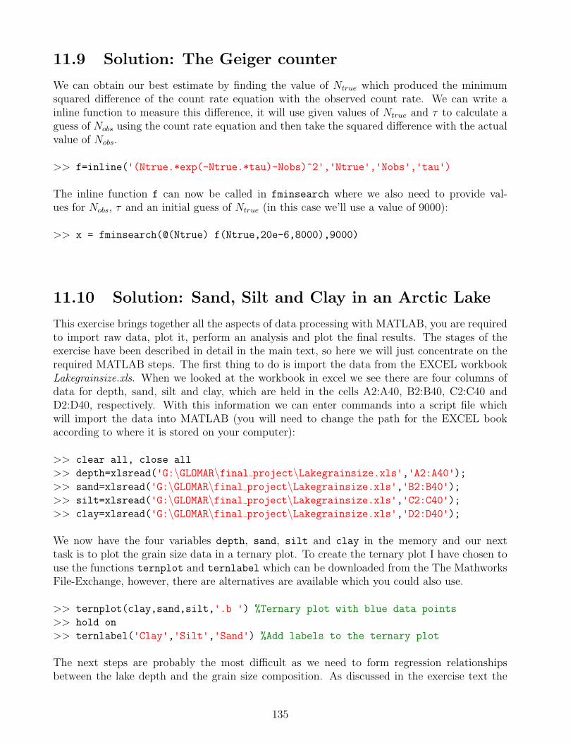
11.9 Solution: The Geiger counter
We can obtain our best estimate by finding the value of Ntrue which produced the minimumsquared difference of the count rate equation with the observed count rate. We can write ainline function to measure this difference, it will use given values of Ntrue and τ to calculate aguess of Nobs using the count rate equation and then take the squared difference with the actualvalue of Nobs.
>> f=inline('(Ntrue.*exp(-Ntrue.*tau)-Nobs)^2','Ntrue','Nobs','tau')
The inline function f can now be called in fminsearch where we also need to provide val-ues for Nobs, τ and an initial guess of Ntrue (in this case we’ll use a value of 9000):
>> x = fminsearch(@(Ntrue) f(Ntrue,20e-6,8000),9000)
11.10 Solution: Sand, Silt and Clay in an Arctic Lake
This exercise brings together all the aspects of data processing with MATLAB, you are requiredto import raw data, plot it, perform an analysis and plot the final results. The stages of theexercise have been described in detail in the main text, so here we will just concentrate on therequired MATLAB steps. The first thing to do is import the data from the EXCEL workbookLakegrainsize.xls. When we looked at the workbook in excel we see there are four columns ofdata for depth, sand, silt and clay, which are held in the cells A2:A40, B2:B40, C2:C40 andD2:D40, respectively. With this information we can enter commands into a script file whichwill import the data into MATLAB (you will need to change the path for the EXCEL bookaccording to where it is stored on your computer):
>> clear all, close all
>> depth=xlsread('G:\GLOMAR\final project\Lakegrainsize.xls','A2:A40');>> sand=xlsread('G:\GLOMAR\final project\Lakegrainsize.xls','B2:B40');>> silt=xlsread('G:\GLOMAR\final project\Lakegrainsize.xls','C2:C40');>> clay=xlsread('G:\GLOMAR\final project\Lakegrainsize.xls','D2:D40');
We now have the four variables depth, sand, silt and clay in the memory and our nexttask is to plot the grain size data in a ternary plot. To create the ternary plot I have chosen touse the functions ternplot and ternlabel which can be downloaded from the The MathworksFile-Exchange, however, there are alternatives are available which you could also use.
>> ternplot(clay,sand,silt,'.b ') %Ternary plot with blue data points
>> hold on
>> ternlabel('Clay','Silt','Sand') %Add labels to the ternary plot
The next steps are probably the most difficult as we need to form regression relationshipsbetween the lake depth and the grain size composition. As discussed in the exercise text the
135

first thing to do is form the log-ratios of the grain size components using clay as the denomi-nator variable:
>> sand clay=log(sand./clay)
>> silt clay=log(silt./clay)
Now we must find the straight-line relationship between the log of depth and the log-ratiosof the grain size components. There are many ways to do this but one of the simplest is touse the function polyfit, which requires 3 inputs, the independent data which in this case isthe log of depth, the dependant data which in this case is the one of the log-ratios, and finallythe order of the polynomial to be fitted (we want a straight-line which is order 1). The outputvariables from polyfit store the structure of the polynomial fit, which for a straight-line is thevalues of the gradient and the intercept.
>> p sand clay=polyfit(log(depth),sand clay,1);
>> p silt clay=polyfit(log(depth),silt clay,1);
In order to draw our regression line representing the relationship between lake depth and grainsize composition we must first define a series of depths that we’ll call D. Then we’ll find thegrain size compositions for the log of these depths according our derived regression relation-ships. This can be done using the function polyval which will evaluate a polynomial withknown coefficients for a given value. You can see in the commands below we supply polyval
with the polynomial coefficients calculated in the previous step and ask it to determine valuesat the logs of the new depth points.
>> D=[1:1:500]; %series of new depths for the model
>> sand clay hat=polyval(p sand clay,log(D)); %log(sand/clay) model
>> silt clay hat=polyval(p silt clay,log(D)); %log(silt/clay) model
Our predictions for the grain sizes are still in the form of log-ratios, but we can convert themback into sand, silt and clay proportions using the equations given in the exercise:
>> sand hat=exp(sand clay hat)./(exp(sand clay hat)+exp(silt clay hat)+1);
>> silt hat=exp(silt clay hat)./(exp(sand clay hat)+exp(silt clay hat)+1);
>> clay hat=1./(exp(sand clay hat)+exp(silt clay hat)+1);
Finally, we just need to add our new regression points as a line in the ternary plot:
>> ternplot(clay hat,sand hat,silt hat,'r') %Add the regression to the plot
136

11.11 Solution: Bringing it all together with cars and
goats
The best way to proceed with the problem is to think how we would play the game once andbuild that into a repeating process so that we can play millions of times and examine the prob-ability of the different results. Lets start with the basic mechanics of the game which we canbreak down into parts, firstly we need to decide on the combination of goats and car which willbe behind the doors. To make this a bit easier we will always use the sequence car-goat-goatand randomly generate the door numbers they are behind. This means we need to produce thenumbers 1,2 and 3 in an random order, which can be done by generating three random numbersand finding the indices which will sort them into ascending (or descending) order, for example:
>> r=rand(3,1);
>> [r,door]=sort(r);
>> door
door =
3
1
2
This means that for this specific game the car would be behind door 3 and goats would bebehind doors 1 and 2. The same process can be combined into a single line:
>>[door,door]=sort(rand(3,1));
We can perform a similar process to obtain the first guess of the contestant, again we’ll generatethe numbers 1,2 and 3 in a random order and take the first number as the guess:
>> [guess,guess]=sort(rand(3,1));
>> guess=guess(1)
guess =
1
So in this case the contestants first guess would be that the car is behind door 1. Now wecan test the first case, did the contestant correctly guess the door in the first instance, if theydid we then have to decide what happens at the next stage, will they stick with their originalchoice, in which case they will win the car, or will they switch, in which case they will win agoat. To represent the choice of wether to switch doors or not we’ll generate a random numberbetween 0 and 1, if the value is <0.5 the contestant sticks with the original door, of the numberis >0.5 they will switch.
switch door=rand(1);
if guess==doors(1) %the correct door was chosen at the beginning
137

if switch door<0.5 %if the number is <0.5 the door isn’t switched
disp('You win a car')
end
end
The opposite situation is a simple extension of this, if the contestant did not originally choosethe correct door then they will only win a car if the value of switch door is greater then 0.5.Therefore both possibilities to win the car can be written as:
switch door=rand(1);
if guess==doors(1) %the correct door was chosen at the beginning
if switch door<0.5 %if the number is <0.5 the door isn’t switched
disp('You win a car')
end
end
if guess∼=doors(1) %an incorrect door was chosen at the beginning
if switch door>0.5 %if the number is >0.5 the door is switched
disp('You win a car')
end
end
We now have the structure of the code with which we can play a single game, but we needto make adjustments so that we can play it repeatedly. If you remember our original questionwe wanted to know if we are more likely to win if we switch doors (which we’ll call a type1 win)rather than sticking with the same door (a type2 win). All we need to do is place the gamesimulation within loop so that we can run it a number of times and add up the number of type1and type2 wins. Finally, we can find the relative probabilities by calculating the total numberof type1 wins compared to the total number of wins.
type1 total=0;
type2 total=0;
for iter=1:1e5
[doors,doors]=sort(rand(3,1));
[guess,guess]=sort(rand(3,1));
guess=guess(1);
switch door=rand(1);
if guess==doors(1) %the correct door was chosen at the beginning
if switch door<0.5 %if the number is <0.5 the door isn’t switched
type2 total=type2 total+1;
end
end
138

if guess∼=doors(1) %an incorrect door was chosen at the beginning
if switch door<0.5 %if the number is >0.5 the door is switched
type1 total=type1 total+1;
end
end
end
prob=type1 total./(type1 total+type2 total)
139