An Introduction to Idempotency - HP LabsAn Introduction to Idempotency Jeremy Gunawardena 1...
50
rhO' HEWLETT An Introduction to Idempotency Jeremy Gunawardena Basic Research Institute in the Mathematical Sciences HP Laboratories Bristol HPL-BRIMS-96-24 September, 1996 The word idempotency siwfies the study of semirings in wmch the addition operation is idempotent: a + a = a. The best-mown example is the max-plus semiring, consisting of the real numbers with negative infinity adjoined in which addition is defined as max(a,b) and multiplication as a+b, the latter being distnbutive over the former. Interest in such structures arose in the late 1950s through the observation that certain problems of discrete optimisation could be linearised over suitable idempotent semirings. More recently the subject has established connections with automata . theory, nonexpanSlVe mappmgs, nonlmear partla differential equations, optunisation theory and large deviations. TIle present paper was commissioned as an introduction to the volume of proceedings for the workshop on Idempotency held at Hewlett Packard's Basic Research Institute in the Mathematical Sciences (BRIMS) in October 1994. It aims to give an introductory survey, from a coherent mathematical viewpoin1 of the recent developments in the subject. iDe major open problems are pointed out and an extensive bibliography is provided. © Copyright Hewlett-Packard Company 1996 Internal Accession Date Only
Transcript of An Introduction to Idempotency - HP LabsAn Introduction to Idempotency Jeremy Gunawardena 1...

rhO' HEWLETT~f..l PACKA~D
An Introduction to Idempotency
Jeremy GunawardenaBasic Research Institute in theMathematical SciencesHP Laboratories BristolHPL-BRIMS-96-24September, 1996
The word idempotency siwfies the study ofsemirings in wmch the addition operation isidempotent: a + a = a. The best-mown example isthe max-plus semiring, consisting of the realnumbers with negative infinity adjoined in whichaddition is defined as max(a,b) and multiplicationas a+b, the latter being distnbutive over the former.Interest in such structures arose in the late 1950sthrough the observation that certain problems ofdiscrete optimisation could be linearised oversuitable idempotent semirings. More recently thesubject has established ~triguing connections withautomata . theory, ~.hscrete e~ent syste~slnonexpanSlVe mappmgs, nonlmear partladifferential equations, optunisation theory and largedeviations. TIle present paper was commissioned asan introduction to the volume of proceedings for theworkshop on Idempotency held at HewlettPackard's Basic Research Institute in theMathematical Sciences (BRIMS) in October 1994.It aims to give an introductory survey, from acoherent mathematical viewpoin1 of the recentdevelopments in the subject. iDe major openproblems are pointed out and an extensivebibliography is provided.
© Copyright Hewlett-Packard Company 1996
Internal Accession Date Only

An Introduction to Idempotency
Jeremy Gunawardena
1 Introduction
The word idempotency signifies the study of semirings in which the additionoperation is idempotent: a + a = a. The best-known example is the max-plussemiring, JR U {-00}, in which addition is defined as max{a, b} and multiplication as a + b, the latter being distributive over the former. Interest in suchstructures arose in the 1950s through the observation that certain problemsof discrete optimisation could be linearised over suitable idempotent semirings. Cuninghame-Green's pioneering book, [CG79], should be consulted forsome of the early references. More recently, intriguing new connections haveemerged with automata theory, discrete event systems, nonexpansive mappings, nonlinear partial differential equations, optimisation theory and largedeviations and these topics are discussed further in the subsequent sectionsof this paper. The phrase idempotent analysis first appears in the work ofKolokoltsov and Maslov, [KM89].
Idempotency has arisen from a variety of sources and the different strandshave not always paid much attention to each other's existence. This has ledto a rather parochial view of the subject and its place within mathematics;it is not as well-known nor as widely utilised as perhaps it should be. Theworkshop on which this volume is based, was organised, in part, to addressthis issue. 'With this in mind, we have tried to present here a coherent account of the subject from a mathematical perspective while at the same timeproviding some background to the other papers in this volume. Vole have saidrather little about what are now standard topics treated in the main booksin the field, [CG79, Zim81, CKR84, BCOQ92, MK94, KMa] and [Mas87a,Chapter VIII]. We have tried instead to direct the reader towards the openproblems and the newer developments, while pointing out the links with otherareas of mathematics. However, we make no pretence at completeness. A different view of the subject is put forward by Litvinov and Maslov in theirsurvey paper in this volume, [LM].
Stephane Gaubert and Jean Mairesse provided the author with extensiveand detailed suggestions on the first draft of this paper. It is a pleasure tothank them, as well as Fran(,;ois Baccelli, Grigori Litvinov, Pierre del Moraland Jacques Sakarovitch, for their comments, which resulted in many corrections and improvements. Any errors or omissions that remain are entirely theresponsibility of the author.

2 Jeremy Gunawardena
2 Dioids
2.1 Introduction
In this section we introduce idempotent semirings, or dioids, and study someof the main examples. As we shall see, dioids occur more widely than onemight suspect and certain classes of dioids have been extensively studiedunder other names. The intention is to give the reader a sense of the scopeof the subject before looking at more specialised topics in later sections.
2.2 Semirings and dioids
We recall that a semigroup is a set with an associative binary operation whilea monoid is a semigroup with a.distinguished identity element, [KS86].
Definition 2.1 A semiring is a set, 8, with two binary operations-denotedwith the usual conventions for addition ("+") and multiplication ("X " or". ")-and two distinguished elements, 0,1 E 8, such that 0 =I 1 and
• (8, +, 0) is a commutative monoid with identity element 0,
• (8, x, 1) is a monoid with identity element 1,
• a.O = O.a = 0 for all a E 8,
• a.(b + c) = a.b + a.c, (b + c).a = b.a + c.a, for all a, b, c E 8.
A dioid, or idempotent semiring, is a semiring, D, such that:
• a + a = a for all a ED.
A commutative dioid is one in which a.b = b.a for all a, bED. A dioid is anidempotent semi-skewfield (respectively, idempotent semifield) if its nonzeroelements form a group (respectively, cor,nmutative group) under multiplication.
The word dioid (or diold) is used by Kuntzmann, [Kun72], to mean simplya semiring or double monoid, a usage followed by others, [GM84]. Thereseems little point in wasting a new word on something well-known and wefollow the modern custom, [BCOQ92, §4.2], of using dioid as a synonym foridempotent semiring.
It is less customary to use + and x to denote the operations in a dioidand many authors use E9 and @. We shall not do so here because, in ourview, formulae involing the latter operations are difficult to read and fail toexploit the analogy with classical algebra. However, our choice does lead to

An Introduction to Idempotency 3
difficulties because some of the best known examples of dioids are based on theclassical number systems and it can be unclear whether, for instance, + refersto the dioid addition or to classical addition. To resolve confusion arisingfrom this, we shall use the symbol := between formulae. This will implythat the symbols on the left hand side refer to the dioid under considerationwhile the symbols on the right hand side have their classical, or customary,meanings. Hence, a x b := a + b, means that dioid mulitipliation is equal tothe customary addition, where customary should be clear from the contextin which the formula appears.
2.3 Examples of dioids
Before going any further, it is best to see some examples.
1. The Boolean dioid: JR = {O, I}, with 0,1 thought of as integers andaddition and multiplication defined as ma..ximum and minimum respectively.
2. The max-plus dioid: lRmax = JR U {-oo} with a + b := ma..x{a, b} anda x b := a + b. Here, 0 := -00 and 1 := O. lRmax is an idempotentsemifield. (So too is JR but for rather trivial reasons!) lRmax sometimesappears in its isomorphic form as the min-plus dioid: lRmin = JRU {+oo},with a + b:= min{a, b} and a x b:= a + b. Here, 0 := +00 and 1 := O.
3. The tropical dioid: Nmin = N U {+oo}, with a + b := min{a,b} anda x b := a + b. Here, 0 := +00 and 1 := O.
4. Let 5 be a set. The set of subsets of 5, P(5), or the set of finite subsetsof 5, p Fin(5), with addition and multiplication defined as union andintersection respectively, are both dioids. Here, 0 := (/) and 1 := 5.Similarly, let T be the set of open sets of any topology with additionand multiplication defined as union and intersection, respectively. ThenT is a commutative dioid. We see that dioids are at least as commonas topological spaces!
5. Suppose that (M,., 1M ) is a monoid. The monoid operation can beused to give P(lvI) or pFin(M) a different dioid structure to that inthe previous example. Addition is still given by union of subsets butmultiplication is defined by: U x V = {u.v I u E U, v E V} whereU, V ~ 1\1. Here 0 := (/) and 1 := {1 M }, There are several interestingexamples of such dioids. Take Al = JRd with the standard vector spaceaddition as the monoid operation. The dioid multiplication in p(JRd)then corresponds to Minkowski addition of subsets, [Hei95]. Anotherexample is the dioid of formal languages. If A is a set, let A* be the setof finite strings (words) over A with the monoid operation defined by

4 Jeremy Gunawardena
juxtaposition of strings and the empty string, t, as the identity element.The subsets of A*, are called (formal) languages over the alphabet A.The dioid P(A*) is noncommutative if A has more than one element.
6. Suppose that (G, +, 0) is an abelian group, not necessarily finite. Forinstance, G = IRn
. Let (~in h(G) denote the set of functions u : G -+~in which are bounded below. If u, v E (~in h(G), define additionpointwise, (u + v)(x) = u(x) + v(x), and multiplication as convolution:(u.v)(x) := infyEG{u(y) + v(x - y)}. Here x - y is calculated in thegroup G. The boundedness of u and v ensures that this is well-defined.(~in h(G) is a convolution dioid, [ST]. The operation u.v is called infconvolution in convex analysis, [Aub93, Exercise 1.4].
7. Let R be a commutative ring and let Spec(R) denote the set of idealsof R. Spec(R) becomes a dioid when addition is defined by the sum ofideals, I +J = {a+b Ia E I, bE J}, and multiplication by the product,I.J = {at.bt + ... + an.bn I ai E I, bj E J}, [Vic89, Chapter 12].
8. If D is a dioid, then Mn (D) will denote the dioid of n x n matrices withentries in D with matrix addition and mulitiplication as the operations.
9. Let D be a dioid and A a set. The dioid of formal power series over Dwith (non-commuting) variables in A, denoted D((A)), is the set of Dvalued functions on A* with addition defined pointwise and multiplication as convolution: if f, 9 E D(A*), then (J.g)(w) = Lu.v=w f(u).g(v).By restricting to the sub-dioid of functions which are non-zero at onlyfinitely many points, we recover the polynomials over D with (noncommuting) variables in A, denoted D(A).
2.4 Homomorphisms and semimodules
Many of the basic concepts in the theory of rings can be defined in a similarway for semirings and can hence be specialised to dioids. For the most part,the idempotency plays no special role. We run through some of the mostimportant definitions here; for more details see [Go192]. The reader who isfamiliar with these elementary concepts might still want to absorb some ofthe notation.
Let R, S be semirings. A homomorphism of semirings from R to S, is afunction f : R -+ S which is a homomorphism of monoids for both additionand multiplication:
f(a + b) = f(a) + f(b)f(a.b) = f(a).f(b)
f(OR) = Osf(1R) = Is .
For example, we can define a function a: P(A*) -+ B((A)) by a(U)(w) = 1if w E U, a(U)(w) = 0 if w rf. U. The reader can check that this is an

An Introduction to Idempotency 5
isomorphism of semirings. That is, there exists a homomorphism of semirings,(3 : lB((A)) -+ P(A*) which is inverse to a: a(3 = IB((A}} and (3a = Ip{A*). Byrestriction, (3 also induces an isomorphism between lB(A) and pFin(A*).
Let (M, +) be a commutative monoid and R a semiring. M is said to be aleft R-semimodule if there is an action of R on M, R x M -+ M, called scalarmultiplication and denoted r.a, such that, for all r, s E R and a, bE M,
r.(a + b)(r + s).a
r.(s.a)
r.(a) + r.(b)r.a + s.a(r.s).a
It is worth noting at this point that if R happens to be a dioid, then M mustnecessarily have an idempotent addition:
a + a = 1.a + 1.a = (1 + l).a = 1.a = a .
A useful source of R-semimodules is provided by the following construction.Let A be any set and let R(A) denote the set of all functions u : A -+ R. Thishas a natural structure as a left R-semimodule: addition is defined pointwise,(u + v)(a) = u(a) + v(a), and scalar multiplication by (r.u)(a) = r.u(a).When A is infinite, R(A) contains inside itself another useful R-semimodule.Define the support of u by supp(u) = {a E A I u(a) =I- O} and let RFin(A)denote the set of functions u with finite support. It is clear that RFin(A) isa sub-semimodule of R(A).
If M, N are R-semimodules, a homomorphism of R-semimodules fromM to N is a homomorphism of monoids f : M -+ N which respects thescalar multiplication: f(r.a) = r.f(a). We can construct homomorphismsbetween the R-semimodules RFin(A) as follows. If f : A -+ B is any setfunction, then f can be extended to a function, also denoted f for convenience, f : RFin(A) -+ RFin(B) where f(u)(b) = LJ(a)=b u(a). The finitenessof supp(u) ensures that this is well-defined. The reader can check that this isa homomorphism of R-semimodules.
At this point, it will be convenient to make use of the language of categorytheory, essentially to clarify the nature of RFin(A). The reader who is unfamiliar with this language but who nevertheless has an intuitive understandingof what it means for an object to be freely generated, will not lose much byignoring the details below. The canonical reference for those wishing to knowmore is MacLane's book, [Mac71].
The constructions given above define a functor from the category of sets,Set, to the category of R-semimodules, SModR , which is left adjoint to theforgetful functor which forgets the R-semimodule structure. That is, if A is aset and M is an R-semimodule, then there is a natural one-to-one correspondence between the respective sets of homomorphisms:
Hom(A, M)set +---+ Hom(RFin(A), M)sModn . (2.1)

6 Jeremy Gunawardena
This expresses the fact that RFin(A) is the free R-semimodule generated byA: any set function f : A -+ M can be extended to a unique homomorphismof R-semimodules f : RFin(A) -+ M. If u E RFin(A), the extension is givenby f(u) = l:aEA u(a)·f(a), the finiteness of supp(u) again ensuring that thisis well-defined.
If M is an R-semimodule then the set Hom(M, lVI)SModR has both an addition, (J + g)(a) = f(a) + g(a), and a multiplication given by compositionof functions (J.g)(a) = f(g(a)). This defines a semiring, over which M isa left semimodule under f.a = f(a). For finitely generated free modules,Hom(M, lVI) is well known. Let A be a finite set, so that RFin(A) = R(A).By (2.1), an element of Hom(R(A), R(A)) is uniquely determined by a function A -+ R(A). This, in turn, may be uniquely specified by a functionA x A -+ R. In other words, by an element of R(A x A), or, after choosingan ordering A = {al' ... , an}, by an n x n matrix over R. It is easy to show,that this gives an isomorphism of semirings, Hom(R(A), R(A)) --t Mn(R).
2.5 The partial order in a dioid
Our constructions have, so far, been valid for arbitrary semirings. The readermight be forgiven for thinking that the theory of dioids has no special character of its own. This is not the case. The idempotency gives rise to a naturalpartial order in a dioid which differentiaties the theory from that of moregeneral semirings.
Proposition 2.1 ([Joh82, §I.1.3]) Let A be a commutative semigroup withan idempotent addition. Define a :::S b whenever a + b = b. Then (A,:::s) isa sup-semilattice (a partially ordered set in which any two elements have aleast upper bound). Furthermore,
max{a, b} = a + b (2.2)
Conversely, if (A,:::s) is a sup-semilattice and + is defined to satisfy (2.2),then (A, +) is an idempotent semigroup. These two constructions are inverseto each other.
It follows that any dioid, D, has a natural ordering, denoted :::S or :::SD.Addition is a monotonic operation and 0 is the least element. Distributivityimplies that left and right multiplication are semilattice homomorphisms; inparticular, they are monotonic.
vVe see from ~roposition 2.1 that a dioid may be thought of as a semilatticeordered semigroup, [Fuc63]. There is a continuing tradition of work on idempotency from this perspective, [CG79, Zim81, But94].
The reader might note that the dioids introduced in §2.3 fall into two mainclasses: those whose partial order is derived from the order on IR. and thosederived from inclusion of subsets.

An Introduction to Idempotency
2.6 Free dioids
7
We turn now to an examination of the dioids arising as sets of subsets (examples 4 and 5 in §2.3). Once again, it is convenient to use the language ofcategory theory.
The constructions P(M) and pFin(M) extend to functors from the category of monoids, Monoid, to the category of dioids, Dioid: if f : M -+ Nis a homomorphism of monoids, then define f : P(M) -+ P(N) by f(U) =
{f(u) Iu E U} and similarly for p Fin (_).
Proposition 2.2 The functor pFin : Monoid -+ Dioid is left adjoint to theforgetful functor from Dioid to Monoid which forgets the dioid addition.
Proof: Let M be a monoid and D a dioid. It is required to show thatthere is a natural one-to-one correspondence between the respective sets ofhomomorphisms:
Hom(M, D) Monoid f---t Hom(pFin(M), D)Oioid .
Let q : M -+ D be a homomorphism of monoids. Define e(q) : pFin(M) -+ Dby e(q)(U) = 2:uE u q(u). It is an exercise to check that e establishes therequired correspondence.
QED
In other words, pFin(M) is the free dioid generated by the monoid M. Theconstruction A * can also be extended to a functor from Set to Monoid which isleft adjoint to the forgetful functor which forgets the monoid multiplication.A * is hence the free monoid generated by A. These constructions can also bespecialised to the commutative case. The free commutative monoid generatedby A is simply NFin (A). By putting these remarks together, we obtain thefollowing characterisations.
Proposition 2.3 ([Gau92, Proposition 1.0.7]) If A is a set, then pFin(A*)is the free dioid, and pFin(NFin(A)) the free commutative dioid ([Shu, Theorem 4.1]), generated by A.
2.7 Quantales
As we saw in §2.4, the difference between P(M) and pFin(M) is similar to thedifference between power series and polynomials. In the former, an infinitenumber of additions can be meaningfully performed. Dioids of this type havebeen extensively studied under another name.
Definition 2.2 A quantale, or complete dioid ([BCOQ92, Definition 4.32]),Q, is a dioid in which the underlying sup-semilattice has arbitrary supremaover which the multiplication distributes: "IS ~ Q and Va E Q,

8 Jeremy Gunawardena
• there exists a least upper bound SUPXES x,.
• a.(suPxES x) = sUPxES(a.x), (SUPxES x).a = sUPxES(x.a) .
The word quantale was coined by Mulvey in his study of the constructivefoundations of quantum theory, [Mul86]. His definition does not require anidentity element for multiplication.
If (V,:::;) is any partial order and S ~ V any subset of V, then it is easyto see that
inf x = sup{y E V I y :::; x, "Ix E S} ,xES
(2.3)
in the sense that, if either side exists, so does the other, and both are equal.Hence, every quantale has a greatest element, T = inf 0 and any subset has aninfimum. However, multiplication does not necessarily distribute over infima,even though it does over suprema.
vVe regard a quantale Q as endowed with an infinitary addition given byLXES x = SUPxES x, following the identification in (2.2). Homomorphismsof quantales are required to preserve the multiplication and the infinitaryaddition. The category of quantales, Quant, forms a subcategory of Dioid.P(-) defines a functor -from Monoid to Quant which is left adjoint to theforgetful functor which forgets the quantale multiplication. Hence, we obtainthe following characterisations.
Proposition 2.4 If A is a set, then P(A*) is the free quantale generated byA ([AV93, Theorem 2.1]) and P(NFin(A)) is the free commutative quantalegenerated by A.
Topological spaces form another source of quantales, as pointed out inexample 4 in §2.3. These quantales are special because multiplication corresponds to minimum. Quantales of this type are called frames, [Joh82,Chapter 2] and are characterised by having 1 as the greatest element and anidempotent multiplication, a2 = a, [JT84, Proposition IIL1]. Because theyprovide an extended concept of topological space, frames have proved important in formulating an appropriate abstract setting-Grothendieck's notionof tapas-for modern algebraic geometry. In the course of proving structuretheorems for topoi, Joyal and Tierney have developed the theory of completesemimodules over frames, [JT84].
Quantales have been studied for a number of reasons. On the one handthe infillitary addition allows the definition of the binary operation a -t b,characterised by C ::5 a -t b if, and only if, c.a ::5 b. (This is best understood as an application of the Adjoint Functor Theorem, [Joh82, §L4.2].)This operation is referred to variously as a residuation, implication or pseudocomplement, [DJLC53, BJ72, Joh82, BCOQ92]. When Q is a frame, the

An Introduction to Idempotency 9
operation -,x = x ---+ 0 has many of the features of a negation, except that thelaw ofthe excluded middle, x+-,x = T may fail. Logicians have consequently
. studied frames as models for intuitionistic logic, [Vic89]. More recently, quantales have served the same purpose for Girard's linear logic. They are alsoused as semantic models in computer science. For details and references, seethe paper by Mascari and Pedicini in this volume, [MP]' or [AV93].
On the other hand, despite the infinitary operation, quantales and framesare still algebraic theories, in the sense that they can be defined in terms ofgenerators and relations, [Joh82, §II.1.2]. For frames, this leads to the studyof topological spaces from an algebraic viewpoint, sometimes called pointlesstopology, [Joh83].
For the purposes of the present paper, quantales are important for thefollowing reason. The discrete dynamical system Xi+! = a,xi + b appears innumerous applications. In general, a may be an element of a dioid D andXi and b elements of some left D-semimodule. The problem is to understandthe asymptotic behaviour of the sequence Xo, Xl, .... A useful first step is todetermine the equilibrium points of the system, where
X = a.x+ b. (2.4)
In a quantale, appropriate equilibrium solutions can always be constructed.(In this volume, Walkup and Borriello consider the more general problem ofsolving a.x + b = c.X + d when a, c E Mn(IRmax ), [WB].)
Definition 2.3 If Q is a quantale and a E Q, the Kleene star of a, denoteda*, is defined by
a* = 1 + a + a2 + a3 + ... = sup a i.
O<i(2.5)
It is sometimes helpful to use also a+ = a + a2 + .". By the infinitarydistributive law, a.a* = a+.
Proposition 2.5 ([Con71, Theorem III.2]) Let Q be a quantale and a, bE Q.Then a*.b is the least solution of (2.4).
Proof: a.(a* .b) + b = a+.b + b = a* .b. Hence a*.b is a solution. Sincemultiplication and addition are both monotonic, if X ::5 y, then a.x + b ::5a.y + b. Now let s be any other solution. Since 0 ::5 s, it follows that b ::5 s.By induction, (1 + a + a2 + ... + an).b ::5 s. It is now not difficult to showthat a*.b ::5 s, as required.
QED
We see from this that a* has a "rational" flavour: it is analogous to (l-a)-1in customary algebra. The star operation satisfies many identities, [Con71 ,Chapter 3], of which we mention only one:
(a + b)* = (a* .b)* .a* . (2.6)

10 Jeremy Gunawardena
The left hand side is a sup of terms of the form ail f)l ... aim f)m. On the righthand side, (a*.b)* is a sup of similar terms except for those ending in powersof a. The product with a* supplies the missing terms. The problem of findinga complete set of identities for +, x and * is very subtle, [Con71, Chapter 12].
The uniqueness of the solution given in Proposition 2.5 appears to be anopen problem. It is a classical result in automata theory, Arden's Lemma,[HU79, Exercise 2.22]' that, in the free quantale, P(A*), if 1 -1. a, then a*.bis the unique solution of (2.4). This is not true in general. In any frame,a2 = a and 1 is the greatest element. Hence the function f(x) = a.x + b isitself idempotent, f2 = f, implying that any element of the form a.x + b isa solution of (2.4). On the other hand, in any quantale, if 1 :::S a, it is easyto see that a*.(u + b) is a solution of (2.4) for any u E Q. Another relevantresult is [BCOQ92, Theorem 4.76].
It is convenient to mention here a technical trick which is well known incertain quarters. It is used by Walkup and Borriello in their paper in thisvolume, [WB], and it will be the key ingredient in the proof of Theorem 3.1.The proof is left as an exercise for the reader, who will need to make use of(2.6) and Proposition 2.5. There are several equivalent formulations: [Kui87,Theorem 2.5],[CMQV89, Lemma 2].
Lemma 2.1 ([Con71, Theorem III.4]) Let Q be a quantale. The followingidentity holds for any block representation of a matrix over Q.
(A B)* = ( (A+BD*C)* A*B(D + CA*B)* )C D D*C(A + BD*C)* (D + CA* B)*
2.8 Matrix dioids and graphs
If the dioid R is not a quantale, it may still be the case that a* exists andthat Proposition 2.5 continues to hold. Indeed, in any dioid, if a :::S 1 thena* = 1. In a matrix dioid, the existence of A* is related to the eigenvaluesof A, in analogy with classical results. For dioids such as Mn(lRmax), this hasbeen completely worked out, [BCOQ92, Theorem 3.17].
The case of matrix dioids is of particular interest for problems of discreteoptimisation. This arises through the intimate relationship between matricesand graphs, which becomes particularly attractive in the idempotent context.Let R be a semiring and T E Mn (R) a matrix.
Definition 2.4 The graph of T, Q(T), is a directed graph on the vertices{I, ... ,n} with edges labelled by elements of R. There is an edge from i to jif, and only if, Tij =1= O. If there is such an edge then its label is Tij .

An Introduction to Idempotency 11
This gives a one-to-one correspondence between n x n matrices over Randdirected graphs on {l,"', n} with edge labels in R.
Taking powers of A corresponds to building longer paths. A path, p oflength m from i to j is a sequence of vertices i = Vo, ... , Vrn = j such thatAV;Vi+l -=I O. We can write
AZi = I:lplw,p
where p runs over all paths of length m from i to j and Iplw is the weightof the path: the product of the labels on the edges in the path, Iplw =
A vov!' ••• • AVm-lVm' For a general semiring, it is hard to deduce much fromthis. If R is a dioid, however, the sum corresponds to taking a maximum withrespect to ~R and Ai; is the maximum weight among paths of length m fromi to j. By choosing the dioid appropriately, a variety of discrete optimisationproblems can be formulated in terms of matrices.
For instance, we can answer questions about the existence of paths in adirected (unlabelled) graph, G. Assume the vertices are labelled {l, .. " n}.Take R = ~ and label each edge of the graph with 1 E~. Let A be the matrixin Mn(~) corresponding to G. Then A* (which exists since ~ and Mn(~) areboth quantales) gives the transitive closure of the edge relation in G: Aij = 1if, and only if, there is some path in G from i to j. Problems of enumeration,shortest paths, critical paths, reliability, etc, in graphs or networks can beformulated using other dioids, often as solutions to (2.4), [GM84, Chapter 2].
To calculate A* efficiently, classical algorithms for computing the inversematrix-Jacobi, Gauss-Seidel, Jordan-can be adapted to the idempotentsetting, [Car7l], [GM84, Chapter2]. For finding longest paths (for which theappropriate dioid is IRmax ) these correspond to well-known algorithms such asthose of Bellman, Ford-Fulkerson and Floyd-Warshall, [Car71].
It is interesting to ask if properties of periodic graphs, which are infinitegraphs with Zn-symmetry, can be studied by similar methods. Backes, in histhesis, has given a formula for longest paths in a periodic graph, [Bac94]. Itseems likely that, at least when n = 1, this can be interpreted in idempotentterms using the matrix methods described above. Can a similiar interpretation be found when n > I?
2.9 The max-plus dioid and lattice ordered groups
The max-plus dioid, IRmax , has been of great importance for idempotency anddeserves special mention. For a general reference see [BCOQ92, Chapter 3].Cuninghame-Green's survey paper, [CG95], discuses several topics that weomit.
As remarked in §2.3, IRmax is an idempotent semifield. The group operationendows such structures with natural symmetry. The reader should have nodifficulty proving the following result by using the remarks in §2.5.

12 Jeremy Gunawardena
Lemma 2.2 If D is an idempotent semi-skewjield then (D, ~D) is a latticeand, for a, bE D\{-oo}, min{a, b} = (a- 1 + b-1)-1.
In the language of ordered algebraic structures, idempotent semi-skewfieldsare therefore lattice ordered groups and these sometimes form a convenientgeneralisation of lRmax. They correspond to the blogs of [CG79], a name whichhas, understandably, not survived.
The most extensively studied aspect of max-plus is linear algebra: finitelygenerated free semimodules and their endomorphisms, [Bap95, BSvdD95,But94, GMb, OR88]. The spectral theory of max-plus matrices has been ofparticular interest because of the role of eigenvalues as a performance measurefor discrete event systems; see §4.4. The basic observation is that eigenvaluescorrespond to maximum mean circuit weights in the associated graph.
Let us consider elements of (lRmax )({I, ... , n}) as column vectors. Recallthat u is an eigenvector of a matrix A E Mn (lRmax ), with eigenvalue A E lRmax ,if Au = AU. If g is a circuit in Q(A)-a path that returns to its startingvertex-let Igle be its length: the number of edges in the circuit. Note that inlRmax , the polynomial equation x k = a has a unique solution: x = a1/ k := a/k.(Dioids with this property are radicable in [CG79] or algebraically completein [MS92].) Hence, the mean weight of a circuit, /l(g) := Iglw/Igle, is a bonajide element of lRmax .
Proposition 2.6 Suppose that A E Mn(lRmax) and Au = AU. Then, inlRmax, A = L-g /l(g), where 9 ranges over circuits of Q(A) whose vertices lie insupp(u). In particular, any two eigenvectors with the same support have thesame eigenvalue.
Results of this type are part of the folklore of idempotency and go back to[CG62], [Rom67] and [Vor67]; the formulation above is taken from [Gun94c,Lemma 4.5]. A great deal more is known, particularly over lRmax, about theexistence of eigenvectors, the structure of the set of eigenvectors, spectralprojectors, etc, [BCOQ92, Chapter 3]. When A is an irreducible matrix (or,more generally, when supp(u) = {I"", n} ), a description of the eigenvectors, valid for radicable idempotent semi-skewfields, appears in [CG79]. Thegeneral case for lRmax is discussed in [WXS90], and later in [Gau92], and fordioids more general than idempotent semi-skewfields in [DSb].
The behaviour of Ak as k ~ 00 is beautifully described by the followingCyclicity Theorem, which asserts that A k is asymptotically cyclic.
Theorem 2.1 ([BCOQ92, Theorem 3.112]) For any matrix A E Mn(lRmax),there exists dEN, such that, Ak+d - Ak ~ 0 as k ~ 00, where subtractionshould be taken in the customary sense.

An Introduction to Idempotency 13
The convergence is with respect to the topology which arises by identifyingRmax with the positive reals, {x E lR. I x > O} under the exponential map:x ---+ exp(x), [BCOQ92, 3.7.4]. (We shall use this identification again in §4.2and will discuss the topology further in §5.4.3.) The asymptotic cyclicity ofA (ie: the least d) can be calculated in terms of the lengths of circuits inQ(A), [BCOQ92, §3.7.1]. The Cyclicity Theorem is one of the main resultsin the linear algebra of Rmax .
The reader may notice here some analogy between the theory of max-plusmatrices and that of nonnegative matrices, as described by Perron-Frobeniustheory, [Min88]. This is one of the most intruiging puzzles in the whole subject. The analogy seems too close to be simply an accident but a satisfactoryexplanation of the relationship has not yet been found. We will return to thispoint in §4.2 and §6.5.
Over a field, every finitely generated module is free but this is not thecase for semimodules over an idempotent semifield. Non-free semimoduleshave been much less well-studied than their free counterparts. Moller, in histhesis, and Wagneur have independently found results which shed light onthe structure of non-free semimodules over dioids like Rmax , [MoI88, Wag91].(See also [JT84].) Further discussion of this appears in Wagneur's paper inthis volume, [Wag].
2.10 Finite dioids
As we have seen, dioids are very plentiful. However, as remarked in §2.5,the examples considered in 2.3 fall into two broad families. It is interestingto speculate on whether this reflects some fundamental underlying classification or is merely an accident resulting from our ignorance. Shubin, whoseems to have been one of the few to take a systematic approach, has constructed all finite commutative dioids having at most 4 elements, [Shu, §2],and has found 14 pairwise non-isomorphic commutative dioids with exactly4 elements. (Conway enumerates certain specialised dioids in [Con71, Chapter 12].) This suggests that dioids are too numerous to expect a simpleclassification. It would, nevertheless, be useful to have a structure theory fordioids to bring some order to this profusion.
In some respects the profusion can be misleading. The following observation, well-known in the theory of lattice ordered groups, [Fuc63, Page 89],shows that there are no idempotent analogoues of the Galois fields.
Proposition 2.7 The only dioid which is both a quantale and an idempotentsemi-skewfield is the Boolean dioid, B. In particular, ([Shu, Theorem 3.1])there are no finite idempotent semi-skewfields other than B.
Proof: Let D be a dioid satisfying the hypotheses and let 9 be the greatestelement of D. Since 1 ::S g, it follows that 9 ::S g2. Hence 9 = g2 and so 9 = 1.

14 Jeremy Gunawardena
Now suppose that 8 =/:. O. Since 8-1 ~ 1, it follows that 1 ~ 8 and so 8 = 1.Hence D = B.
QED
This negative result is an appropriate place to bring this section to a close.We hope to have given some idea of the scope of the dioid concept. It would befair to say that most of the interesting questions about general dioids remainunanswered, if not unasked. In the subsequent sections we shall be concernedwith specific dioids and will not touch on such general matters again.
3 Automata and idempotency
Automata may be thought of as language recognisers. That is, as rules forrecognising strings of symbols from some (finite) alphabet. By defining appropriate rule schemes, computer scientists have defined classes of automatafinite automata, push-down automata, stack automata, Turing machines, etc,[HU79]-and corresponding classes of languages, [Sal73]. Because languagesare elements of the free quantale, P(A*), it should not come as a surprisethat automata theory has something to tell us about idempotent semirings.In this paper, we shall only consider finite automata, where the connectionshave been most studied. For a good overview see [Per90].
Our main objective in this section is to prove a generalisation of Kleene'sTheorem, [Kle]. This is the starting point of finite automata theory and itappears in several papers in this volume, [Kro, Pin]. We then discuss brieflythe way in which the tropical dioid has been used to solve certain decisionsproblems of finite automata.
3.1 Quantales and Kleene's theorem
It will be convenient to identify an element u E B({I, ... ,n}) with a column vector, as in §2.9, and to make use of the customary operations onvectors and matrices. For instance, u t will denote the transpose of u:ut = (u(l),"', u(n)). Since the Boolean dioid, 1m, can be regarded as asubdioid of any dioid, D, vectors and matrices over B can always be regardedas vectors and matrices over D.
Definition 3.1 Let Q be a quantale and S ~ Q. An element q E Q is recognisable over S if, for some n, there exists a matrix T E Mn(S), and vectorsL, ¢ E B({I, ... ,n}) such that q = LtT*¢. The set of element8 recognisableover S will be denoted Rec(S).
Let A be a finite set and let Q = P(A*), the free quantale generated byA. The elements of Q are the languages over A. Let S = {q E Q I q ~ A},

An Introduction to Idempotency 15
where A is treated as an element of Q by identifying each a E A with thecorresponding string of length 1. The elements of S can then be identified withthe subsets of A. The data (l" T, ¢» over S correspond to a nondeterministicfinite automaton, [Pin, §5.1]. The states of the automaton are {I"", n} andthe subsets l, and ¢> are the initial states and final states, respectively. Tencodes the transitions of the automaton: if Tij = q, where q ~ A, then ifthe automaton is in state i and encounters any symbol from the subset q,it may make a transition to state j. The possibility that the same symbolcould occur in both Tij and Iik, where j =1= k, or that Iij = 0, allows fornondeterminism.
In the usual definition of a finite automaton, the effect of individual symbols is separated out. Let j.L : A , Mn(lB) be given by: j.L(a)ij = 1 if, andonly if, a E Iij. The matrix j.L(a) identifies those transitions which recognisethe symbol a. It follows that, in Mn('P(A*)),
T = L (aI)j.L(a) ,aEA
where I is the identity matrix. Since Mn(lB) is a multiplicative monoid, thefunction j.L can be extended to a homomorphism of monoids j.L : A* , Mn(B).Hence, ignoring initial and final states, we can think of an automaton indifferent ways: as a representation of the free monoid over finitely generatedfree B modules, or as a finitely generated semigroup (or monoid) of matricesgenerated by the subset {j.L(a) I a E A} ~ Mn(lB). The slogan automata aresemigroups of matrices is helpful to keep in mind, particulary when it comesto defining more general types of automata, as in §3.2 and §4.1.4.
vVhat does the element q = l,tT*¢> correspond to in terms of automata?Recalling the discussion in §2.8 the reader can check that T[j is the set ofstrings of length m which lead from state i to state j. It follows that q is theset of strings of any length which lead from some initial state to some finalstate. Hence, q is the language recognised by the automaton, [Pin, §5.1].
Kleene's original result, [Kle], which is the starting point offormallanguagetheory, characterised the languages of finite automata; it was stated, in effect,for the free quantale, P(A*). Following Conway, [Con71], we state and proveit for an arbitrary quantale.
Definition 3.2 Let Q be a quantale and S ~ Q. The rational closure of S,S*, is the smallest subset of Q which contains S and is closed under +, xand *.
Theorem 3.1 Let Q be a quantale and {O, I} ~ S ~ Q. Then Rec(S) = S*.

16 Jeremy Gunawardena
Proof: We first show that 8* ~ Rec(8). Choose s E 8 and form the databelow, which we may do since 0 E S.
Evidently, [}T*¢ = s and so 8 ~ Rec(8). Now suppose that ql = £lTt¢l andq2 = £2T2¢2 and form the three sets of block matrix data below, which wemay do since {O, I} ~ S.
(It is instructive to picture these constructions for finite automata.) Thereader can now check, using Lemma 2.1, that £tT*¢ for each set of data is,respectively, ql +q2, ql.q2 and q~. It follows by induction that Rec(S) is closedunder +, x and *. Hence, S* ~ Rec(S), since S* is the smallest set containingS with that property.
For the other way round, if q = £T*¢, where T E Mn(8), then, byLemma 2.1, T* E Mn(S*). Hence q E S*. It follows that Rec(S) = 8*,as required.
QED
There is a mild embarassment with this result: in the case of finite automata, where Q = P(A*) and S = {q ~ A}, 1 tJ. S! However, in this case, Shas additional properties that allow the same result to go through.
Corollary 3.1 Let Q be a quantale and 8 ~ Q. If 0 E 8 and 8 is closedunder +, then Rec(8) = 8*.
Proof: By the Theorem, Rec(8U{1}) = (8U{1})*. Choose q E 8U{1} andsuppose that q = £tT*¢ where T E Mn(8 U {I}). We can write T = C + Pwhere C E Mn(lll) and P E Mn(S). By (2.6),
q = £t(C + P)*¢ = £t(C* P)*(C*¢).
Since 8 is closed under +, C* P E Mn(8) and, evidently, C*¢ E $({I, ... ,n}).Hence, q E Rec(8) and so Rec(8U{1}) = Rec(8). Furthermore, since 0 E S,it is easy to see that (8 U {l})* - 8*. Hence, Rec(8) = 8*.
QED
The treatment we have given follows Conway, [Con71], and was also influenced by Kuich, [Kui87], who states the result in even greater generality. The

An Introduction to Idempotency 17
essential ideas, but not the theorem itself, can be found in [CMQV89], whichinexplicably fails to make any reference to the automata theory literature.
As we saw in §2.4, the free quantale, P(A*), can also be thought of asthe power series ring lR((A)). Schutzenberger has extended Kleene's resultto power series rings, R((A)), where R is a semiring which is not necessarilyidempotent. The * operation cannot now be defined on all of R((A)) butdoes exist on those series whose constant term is O. This result, known as theKleene-Schutzenberger Theorem, is discussed further in Krob's paper in thisvolume, [Kro, §2.2].
It is rather peculiar that there are two generalisations of Kleene's originalresult, in one of which idempotency plays a crucial role while in the otherit is the free monoid structure of A*. It would be very interesting to have asingle formulation which includes both contexts and yet retains the clarity ofKleene's original result.
3.2 The tropical dioid
The star operation is not a simple one because of its infinitary nature. It isinteresting to ask when it can be defined in a finite way. That is, whether
a* = 1 + a + ... + am, for some m. (3.1)
In a dioid which is not a quantale, this gives a way of constructing a*; Gondranand Minoux introduced the notion of m-regularity, am+! = am, for just thisreason, [GMb, Definition 1]. In automata theory, (3.1) is known as the finitepower property. In 1966, Brzozowski raised the question of whether it wasdecidable if a given rational set (ie: the language of a finite automaton) hadthis property.
This celebrated problem was solved in the affirmative independently by Simon, [Sim78], and Hashiguchi, [Has79]. Simon's proof introduced the tropicaldioid, Nmin , into automata theory and initiatied a deep exploration of decision problems related to the * operation. For an early survey, see [Sim88].The basic idea is to use automata with multiplicities in Nmin or, equivalently,semigroups of matrices in Mn(Nmin ), to reformulate the finite power propertyas a Burnside problem. Recall that the original Burnside problem asks if afinitely generated group must necessarily be finite if each element has finiteorder. This is true for groups of matrices over a commutative ring but is falsein general. An essential step in Simon's proof is to show that it is also truefor semigroups of matrices over Nmin , [Sim78, Theorem C).
For further details, the reader cannot do better than turn to the papersin this volume devoted to this subject. The tutorial by Pin, [Pin], explainsin more depth how the tropical dioid enters the picture, while that of Krob,[Kro], surveys a number of decision problems related to (3.1). D'Alessandroand Sakarovitch show that the finite power property also holds for rational

18 Jeremy Gunawardena
subsets of the free group, [dSa]. Leung, in his thesis, introduced topologicalideas into the study of * problems over the tropical dioid. His paper in thisvolume gives a new and simplified treatment of this approach, [Leu].
Gaubert has initiated the study of automata with multiplicities in lRmax andhas shown that the Burnside problem has a positive answer for semigroups ofmatrices in Mn(lRmax), [Gau]. The rationale for introducing such automatais that, just as the tropical dioid can be used to estimate frequencies (howoften?), max-plus can be used to estimate durations (how long?). This leadsnaturally to the next section which studies problems of performance analysis.We move, correspondingly, from P(A*) and Nmin to lRmax.
4 Discrete Event Systems
4.1 Introduction
4.1.1 Examples and general questions
A discrete event system is one whose behaviour consists of the repeated occurrence of events, [Ho89, Scanning the Issue]. For example: a distributedcomputing system, in which an event might be the receipt of a message; adigital circuit, in which an event might be a voltage change on a wire; or amanufacturing process, in which an event might be the delivery of a part toa machine.
Our main interest will be in the long-term behaviour of the system. Ifa denotes an event and t i (a) denotes the time at which the i-th occurrenceof this event takes place then we shall study the asymptotic behaviour ofthe sequence t1(a), t2(a),···. Depending on the nature of the system, thisquestion may have to be formulated stochastically: the ti(a) would then berandom variables over some suitable measure space. This form of randomnessis that of a random environment, as distinct from the additive noise that iscustomary in signal processing or linear systems theory.
It may not be immediately obvious that idempotency has anything tocontribute to this. In fact, discrete event systems which can be modelledby max-plus matrices have been studied repeatedly, [CG62, Rei68, RH80,CDQV85, Bur90, RS94, ER95], although not all these authors have explicitlyused the idempotency. In this volume, Giirel, Pastravanu and Lewis use maxplus matrices to study manufacturing systems, [GPL); Cofer and Garg exploitthe partial order structure of lRmax to study supervisory control, [CGa]; andCuninghame-Green uses polynomials over max-plus to study the realisabilityproblem, [CGb).
There are many questions that can be asked about the long-term behaviourof discrete event systems. We shall consider only a few. Do there exist steady

An Introduction to Idempotency 19
or periodic regimes? What form do they take? On average, how quickly doesthe next occurrence of a take place?
4.1.2 Mathematical models for DES
To answer questions such as those above, it is necessary to have a mathematical description of the system, which specifies a mechanism for determiningwhen events occur. A variety of models have been proposed, [H089]. Theautomata of the previous section are convenient for modelling systems withstate. They allow easy specification of how different choices of event canoccur, depending on the current state of the system. To specify temporal behaviour, they can be augmented with information on the duration of events,as in the model proposed by Glasserman and Yao, [GY94]. A different approach is to specify how events are causally related to each other. An exampleof this is the classical Gantt chart, or PERT diagram. A somewhat relatedmodel is the task-resource model, studied by Gaubert and Mairesse in thisvolume, [GMa], in which tasks are specified by their durations and the resources they require. This is sometimes called a tetris model by analogy withthe computer game of that name.
In the tetris model, resources are renewable and can be used repeatedly,like a machine in a factory. For consumable resources, a more complex modelis required, which combines both state and causal aspects. Petri nets haveproved popular in this respect, [Rei85]. A Petri net can be defined in termsof a finite set of tasks, Q, and a finite set of resource types, P. Each task, q,consumes and produces a basket of resources, which are specified as elements"q, q", respectively, of N(P). The state of the system is given by an element,c E N(P)' which specifies the current availability of resources of each type.The only tasks, q, which can proceed in state c are those for which thereare sufficient resources, ie: "q ~ c; if q does proceed, the state of the systemchanges to c - "q + q". (Inequality and addition being defined, as usual,pointwise in the semimodule N(P).) Temporal behaviour can be incorporatedby, for instance, giving each resource a holding time for which it must be kept,before becoming available for consumption by a task. Timed Petri nets arethe subject of the paper by Cohen, Gaubert and Quadrat in this volume,[CGQ].
Suppose that in a timed Petri net, for each resource, there is exactly onetask which produces it and exactly one task which consumes it. Such a netcan be described by a directed graph in which the vertices correspond tothe tasks and the edges correspond to the resources. For obvious reasons,this is known as a timed event graph. Its importance lies in the fact that itstemporal behaviour can be completely described as a linear system over lRmax ,[BCOQ92, §2.5]. That is, if x(k) denotes the vector of k-th occurrence timesof the different tasks in the net, then, under reasonable conditions, there exist

20 Jeremy Gunawardena
matrices Ao, ... ,Ap E Mn(JRmax ), such that, for sufficiently large k,
x(k) = Aox(k) + A1x(k - 1) + ... + Apx(k - p) .
This result, that timed event graphs are linear systems has been the key toan algebraic approach, based on idempotency, to the study of discete eventsystems, [CDQV85, CMQV89]. The spectral theory of max-plus matrices, asdiscussed in §2.9, and such results as the Cyclicity Theorem, Theorem 2.1,enable one to draw important and useful conclusions about the long-termbehaviour of the timed event graph.
The linear theory also has implications for efficient simulation of discreteevent systems. The discrete event simulators currently used for performancemodelling in industry take no account of the underlying algebraic structure.However, as shown in [BC93], this can be used to develop more efficientsimulation algorithms.
The main limitation of event graphs is their inability to capture conflict,or competition for resources. Each resource in the event graph is consumedby only one task. Tasks may proceed in parallel but they cannot pre-empteach other. (A finite automaton, in contrast, allows a choice among differentoutcomes.) Free choice nets are a class of Petri nets which include eventgraphs but allow some conflict, [DE95]. If there is a hierarchy of Petri netmodels then free choice nets are the obvious candidate for the next level ofcomplexity beyond event graphs. In the untimed case they are known tohave many interesting properties, [DE95]. In the timed case, the results of[BFG94] confirm that, at least from a mathematical standpoint, free choicenets are a good class to study.
It is clear from this discussion that there are a variety of different modelsfor studying discrete event systems. There is not much consensus on a singlefundamental model, [Ho89, Scanning the Issue]. Our approach in the rest ofthis section will be to extract certain features which appear both conceptuallyreasonable and common to many systems, and to study a basic model withjust these features. This basic model, of topical functions, will include as aspecial case the linear theory based on max-plus. It can also be extended inseveral ways and used as a building block to model a wide class of discreteevent systems. As we shall see, there are many unanswered questions aboutthe basic model itself.
4.1.3 The basic model
Let lRn denote the space offunctions lR(l,' .. ,n), which we think of as columnvectors. We use x, y, z for vectors and Xi instead of x(i) for the i-th componentof x. lRn acquires the usual pointwise ordering from the ordering on lR: x :S yif, and only if, Xi :S Yi for 1 :S i :S n. If x E lRn and h E lR then x + h willdenote the vector Y for which Yi = Xi + h: the operation is performed on each

An Introduction to Idempotency 21
component of the vector. This vector-scalar convention extends to equationsand inequalities: x = h will mean that Xi = h for 1 ~ i ~ n.
Definition 4.1 ([GK95]) A topical junction is a junction, F : jRn -+ jRn, suchthat, ij x, y E jRn and h E jR, then the jollowing properties hold:
• monotonicity X ::; y ===> F(x) ::; F(y)
• (homogeneity) F(x + h) = F(x) + h.
M
H
A topical function can be thought of as modelling a system with n eventsin which x E jRn specifies the time of occurrence of each event and F(x)specifies the times of next occurrences. The sequence x, F(x), F2(x),'" isthen the sequence of occurrence times of events, whose asymptotic behaviouris the object of study. Definition 4.1 can be understood as follows: if thetimes of occurrences of some events are increased, then the times of nextoccurrences of all events cannot decrease; if the times of occurrences are allincreased, or decreased, by exactly the same amount for each event, then sotoo, respectively, are the times of next occurrences. These properties appearvery reasonable and can be seen to hold in some form for most discrete eventsystems.
Functions satisfying the conditions of Definition 4.1 have been introducedand studied independently by other authors, [Kola, Vin], but the materialdiscussed below, as well as the name topical, is based on joint work of thisauthor with Keane and Sparrow, [GK95, GKS97].
4.1.4 Extensions of the basic model
There are practical systems which can be modelled directly as topical functions, [Gun93, SS92], but such systems are rather restricted. They mustusually be closed, or autonomous, in that they require only an initial condition to generate a sequence of occurrence times. Open systems, in contrast,require input to be regularly provided. To model this, it is more convenient towork, not with vectors in jRn, but with appropriate functions jR -+ jRn, whichrepresent input, or output, histories. This requires an extension of the theory of topical functions to infinite dimensional spaces, a problem studied in[Kola]. Another extension is to study semigroups of topical functions, whichallows one to model the choice or conflict described in §4.1.2. As remarkedat the end of §3.2, Gaubert has made initial investigations in this direction,[Gau]. Finally, stochastic systems can be modelled by random variables taking values in the space of topical functions. In this volume, Baccelli andMairesse give an extensive discussion of ergodic theorems for random topicalfunctions and for more general systems, [BM], while Gauajal and Jean-Marie

22 Jeremy Gunawardena
study the problem of computing asymptotic quantities in stochastic systems,[GJM].
These three extensions bring a much wider class of discrete event systemswithin our scope. It remains an open problem to understand exactly howmuch wider. For instance, how can Petri nets be incorporated in this framework? What about the model of Glasserman and Yao?
Before going further, we need to see some concrete examples. We shall thendiscuss the properties of topical functions, with reference to the questionsraised in §4.1.1.
4.2 Examples of topical functions
Let Top(n, n) denote the set of topical functions, F : IRn -+ IRn. This set
has a rich structure, which we need some notation to explain. If a, bareelements of some partially ordered set, let a V b and a /\ b denote the leastupper bound and greatest lower bound, respectively, when these exist. Theset of functions, IRn -+ IRn has a natural partial order defined pointwise fromthat on IRn . Finally, let F- denotes the function -F(-x).
Lemma 4.1 ([GK95, Lemma 1.1]) Let F, G E Top(n, n). Let A, Jl E IR satisfyA, p ~ 0 and A + p = 1. Let c E IRn
. Then FG, F V G, F /\ C, F + c, F- andAF + pC E Top(n, n).
This result is an immediate consequence of Definition 4.1. Top(n, n) is adistributive lattice under V and /\. It is almost a Boolean algebra with Fas complement but lacks top and bottom elements.
Definition 4.2 A function F : IRn -+ IRn is said to be simple if each component, Fi : IRn -+ IR, can be written as Fi(x) = Xj + a, for some j and somea E R
Simple functions are clearly topical. Lemma 4.1 now provides a mechanismfor building topical functions which are not simple.
Definition 4.3 ([Gun94c]) A function F : IRn -+ IRn is said to be min-max ifit can be constructed from simple functions by using only V and /\. Such afunction is max-only if it can be built using only V and min-only if it can bebuilt using only /\.
Max-only functions provide the link to idempotency. Any max-only function can be placed in normal form:

An Introduction to Idempotency 23
where A E Mn(JRmax ). We may then write F(x) = Ax. Hence, max-onlyfunctions correspond to matrices over lRmax which satisfy the non-degeneracycondition:
Vi, 3j, such that Aij =J -00 . (4.1)
A min-only function, dually, corresponds to a matrix over lRmin' Min-maxfunctions are nonlinear in the idempotent sense.
Lemma 4.2 ([GKS97]) Choose F E Top(n, n) and a E IRn . There exists amax-only function Fa such that F(a) = Fa(a) and F ~ Fa. A dual statementholds for min-only functions.
Corollary 4.1 ([GKS97]) Let F E Top(n, n). Then F can be written in thetwo forms:
1\ Gi = F = VHjiE[ jEJ
(4.2)
where Gi are max-only, H j are min-only and I and J may be uncountablyinfinite.
Min-max functions are, in a strict sense, finite topical functions. If either ofthe index sets, lor J, is finite, then F is a min-max function. In this case, therepresentations in (4.2) can be reduced to essentially unique normal forms,[Gun94c, Theorem 2.1]. Min-max functions capture some of the dynamicalfeatures of topical functions; see Corollary 4.2.
The infinite topical functions include some well-known functions in disguise. Let IR+ denote the positive reals and lR+o the nonnegative reals. Letexp : IRn -t (1R+)n and log: (1R+)n -t IRn be defined componenentwise:exp(x)j = exp(xi) and log(x)i = log(xi)' These are mutually inverse bijections between IRn and (1R+)n. Let A : (1R+)n -t (1R+)n be any function onthe positive cone and let E(A) : IRn -t IRn denote the function log(A(exp)).The functional E allows us to transport functions on the positive cone to functions on IRn . Moreover, E(AB) = E(A)E(B), so A and E(A) have equivalentdynamic behaviour.
Now suppose that A is a nonnegative matrix, A E Mn (IR+O), which satisifesa similiar non-degeneracy condition to (4.1): Vi, 3j, such that Aij =J O.Then A preserves the positive cone, when elements of (1R+)n are interpretedas column vectors in the usual way. The reader can easily check that E(A)is a topical function. It follows that the theory of topical functions is ageneralisation of Perron-Frobenius theory, [Min88]. It can further be shown,using Lemma 4.1, that a number of problems considered in the optimisationtheory literature also fall within the theory of topical functions, [GKS97].These include problems of deterministic optimal control, Markov decisionprocesses and Leontief substitution systems.

24 JerenlY Gunawardena
4.3 N onexpansiveness and perioidicity
If x E JRn, let II x II denote the £00 norm of x: II x II = vl~i~nlxil. A functionF : JRn --+ JRn is nonexpansive in the £00 norm if
• II F(x) - F(y) II ::; II x - y II . N
The following observation was first made by Crandall and Tartar, [CT80]; seealso [GK95, Proposition 1.1] for a proof adapted to the present context.
Proposition 4.1 If F : JRn --+ JRn satisfies H, then M is equivalent to N.
In particular, topical functions are nonexpansive. This constrains their dynamics in ways that are still not understood. We draw the reader's attentionhere to one result which has significance for discrete event systems.
One of the general questions raised in §4.1.1 concerned the existence of aperiodic regime. In the light of the suggested interpretion of topical functionsin §4.1.3, a periodic regime can be reasonably formulated as a generalisedperiodic point: a vector x such that FP(x) = x + h for some p > 0 andsome h E JR. (Recall that we are using the vector-scalar convention of §4.1.3.)The system returns after p occurrences with a shift of h in each occurrencetime. Because of property H, this behaviour persists. We can, without lossof generality, consider only ordinary periodic points, because FP (x) = x + hif, and only if, (F - hlp)P(x) = x and, by Lemma 4.1, F - hlp is topical.
The least p for which FP(x) = x is the period of F at x. What periods arepossible for discrete events systems modelled by topical functions? It turnsout, surprisingly, that there is a universal bound on the size of periods whichdepends only on the dimension of the ambient space.
Theorem 4.1 ([BW92]) If F : JRn --+ JRn is nonexpansive in the £00 norm andifp is the period of a periodic point of F, then p::; (2n)n.
Results of this form originate in the work of Sine, [Sin90]. An up to datediscussion, as well as complete references, can be found in the survey paperby Nussbaum in this volume, [Nus]. The bound in Theorem 4.1 is not tight:Nussbaum has conjectured that p ::; 2n , and this can be shown to be bestpossible. The Nussbaum Conjecture has been proved only for n ::; 3 andremains the outstanding open problem in this area.
For topical functions, more can be said. The following is an immediateconsequence of Lemma 4.2.
Corollary 4.2 ([GKS97]) Let F be a topical function and S ~ JRn any finiteset of vectors. There exists a min-max function G such that F(s) = G(s) forall s E S. In particular, any period of a topical function must be the periodof a min-max function.

An Introduction to Idempotency 25
It follows that it is sufficient to consider only min-max functions in determining the best upper bound for the periods of topical functions. Byaugmenting min-max functions with F(-x), where F is min-max, it is possible to give a similar reduction for general nonexpansive functions, [GKS97].Gunawardena and Sparrow, in unpublished work, have shown that there aremin-max functions in dimension n with period nqn/2] and conjecture thatthis is the best upper bound for topical functions.
Fixed points, where F(x) = x, are of particular importance for discreteevent systems. They represent equilibria, as in (2.4). The existence of fixedpoints for nonexpansive functions is a classical problem, [GK90]. For topicalfunctions, Kolokoltsov has given a sufficient condition in terms of a gametheoretic representation of topical functions, [Kola, Theorem 9]. For minmax functions, much stronger results are thought to hold, as in Theorem 4.3.This turns out to be related to the other question raised in §4.1.1, whichforms the subject of the next section.
4.4 Cycle times
The rate at which events occur in a discrete event system is an importantmeasure of its performance. The average elapsed time between occurrences,starting from the initial condition x E ~n, is given by (Fk(x) - Fk-1x + ... +F(x) - x)/k. The asymptotic average, as k ~ 00, is then
lim Fk(x)/k .k~oo
(4.3)
It is not at all clear that this limit exists in general. Suppose, however, thatit does exist for a given F at some initial condition x and that y is someother initial condition. Since F is nonexpansive, II Fk(x) - Fk(y) II ~ II x - y II.Hence, if the limit (4.3) exists anywhere, it must exist everywhere, and musthave the same value.
Definition 4.4 Let F E Top(n, n). The cycle time vector of F, X(F) E lRn ,
is defined as the value of (4.3) if that limit exists for some x E lRn, and is
undefined otherwise.
If F has a generalised fixed point, F(x) = x + h then, by property H,Fk(X) = X + kh. Hence, X(F) = h. If F is a max-only function, andA ElvIn (lRmax ) is the corresponding max-plus matrix, then a generalised fixedpoint of F is simply an eigenvector of A and h is the corresponding eigenvalue.By Proposition 2.6, h is the largest mean circuit weight in Q(A). Similarly,if F = E(A), where A E lvIn(lR+O) , then exp(x) E (lR+)n is an eigenvector ofA with eigenvalue exp(h). In this case exp(h) is the classical spectral radiusof A. We see from this that X(F) is a vector generalisation of the notion ofeigenvalue, suitable for an arbitrary topical function.

26 Jeremy Gunawardena
However, if A E Mn(lRmax) is the max-plus matrix corresponding to themax-only function F, then not all eigenvectors of A can be generalised fixedpoints of F. They must lie in jRn and hence have no component equal to-00. To bring the other eigenvectors into the picture, requires some formof compactification of jRn, analogous to putting the boundary on the positivecone (jR+)n. It also suggests the existence of other cycle time vectors whichgive information on fixed points lying in different parts of this boundary. Tomake sense of this for topical functions remains an open problem.
When does X(F) exist? The first indication that this is a difficult questioncame from the following result of Gunawardena and Keane.
Theorem 4.2 ([GK95]) Let {ai}, i 2 1, be any sequence of real numbersdrawn from the unit interval [0,1]. There exists a function F E Top(3, 3),such that Fi(O, 0, 0h = al + ... + ai.
In particular, X(F) does not always exist and the result indicates the extentof the departure from convergence.
On the other hand, there is strong evidence that X(F) does exist for minmax functions. We can formulate this by asking how X(F) should behave withrespect to the operations which preserve min-max functions. Let MM(n, n) ~Top(n, n) denote the set of min-max functions jRn -+ jRn. It is easy to seethat MM(n, n) is closed under all the operations of Lemma 4.1, with theexception of convex combination: >...F + J.LG. In particular, MM(n, n) is adistributive lattice. MM(n, n) also has a Cartesian product structure in whicheach F E MM(n, n) is decomposed into its separate components (FI , ... ,Fn ).
If 5 ~ Al X ... x An is a subset of some such product, let r(S) denote itsrectangularisation:
r(S) = {u E Al X ... x An l1rk(U) E S},
where 1rk : Al X ... x An -+ A k is the projection on the k-th factor. It isalways the case that S ~ r(S) and if S = r(S) we say that S is a rectangularsubset. For example, if F, G E MM(2, 2) then
The lattice operations on MM(n, n) behave well with respect to the Cartesianproduct structure: if S ~ MM(n, n), then
V F = V G andFES GEr(S)
/\ F = /\ G.FES GEr(S)
(4.4)
Conjecture 4.1 (The duality conjecture) X : MM(n, n) -+ jRn always existsand is a homomorphism of lattices on rectangular subsets: if S ~ MM(n, n)

An Introduction to Idempotency
is a finite, rectangular subset, then
X( VF)FEB
X( 1\ F) -FES
VX(F)FEB
1\ X(F) .FES
27
Theorem 4.3 ([Gun94a]) Let F E MM(n, n). If the duality conjecture istrue in dimension n then F (x) = x + h for some x, if, and only if, X(F) = h.
Conjecture 4.1 was first stated in a different but equivalent form in[Gun94a]. By virtue of (4.4), it gives an algorithm for computing X(F) forany min-max function in terms of simple functions, for which Xcan be trivallycalculated. However, because of the rectangularisation required in (4.4), thisalgorithm is very infeasible. This raises issues of complexity about whichlittle is known.
The conjecture is known to be true when S consists only of simple functions. That is, when VFEB F is a max-only function, and /\FEB F is a min-onlyfunction. The conjecture has also been proved in dimension 2, where the argument is already non-trivial, [Gun94b]. Sparrow has shown that X exists formin-max functions in dimension 3 but his methods do not establish the fullconjecture, [Spa96]. The duality conjecture remains the fundamental openproblem in this area and a major roadblock to further progress in understanding topical functions.
The existence of Xdoes not depend on the finiteness of min-max functions:it also exists for functions &(A) where A E Mn(lR+O), [GKS97]. At present,we lack even a conjecture as to which topical functions have a cycle time.
We have sketched some of the main results and open problems for topicalfunctions, which we believe are fundamental building blocks for discrete eventsystems. Topical functions also provide a setting in which max-plus linearity,A E Mn{lRmax ), and classical linearity, A E Mn(IR+O), coexist. As we menti::>ned in §2.9, the relationship between these is a very interesting problem.We shall to return to it in §6.5. Before that, we must venture into infinitedimensions.
5 Nonlinear partial differential equations
5.1 Introduction
In this section we shall be concerned with scalar nonlinear first order partialdifferential equations of the form
F(x, u(x), Du(x)) = 0 (5.1)

28 Jeremy Gunawardena
where F : JRn x JR x JRn -+ lR. Here, u is a real-valued function on some opensubset X ~ JRn , u : X -+ JR, and Du(x) E JRn can be thought of as thederivative of u at x, Du = (aU/aXI,'" ,au/axn ).
It may seem implausible that idempotency has anything to say about differential equations: operations like max(u, v) do not preserve differentiablefunctions. However, remarkable advances have taken place in our understanding of nonlinear partial differential equations which enable us to give meaningto solutions of (5.1) which may not be differentiable anywhere. From one perspective, this can be viewed as borrowing ideas from convex analysis. Indeed,the origins of the differential calculus itself go back to Fermat's observationthat the ma"'Cimum of a function f : JR -+ JR occurs at points where df / dx = O.Efforts to generalise this to non-differentiable functions have led to new notions of differentiability, [Aub93, Chapter 4], which are closely related to theideas discussed below, [CEL84, Definition I]. For ease of exposition, we takea different approach, but convex analysis forms a backdrop to much of whatwe say and its relationship to idempotency is badly in need of further investigation. Aubin's book provides an excellent foundation, [Aub93].
5.2 Viscosity solutions
The advances mentioned above centre around the concept of viscosity solutions, introduced by Crandall and Lions in a seminal paper in 1983 followingrelated work of Kruzkov in the late 1960s. For references, see the more recentuser's guide of Crandall, Ishii and Lions, [CIL92], which discusses extensionsof the theory to second order equations. The earlier survey by Crandall,Evans and Lions, [CEL84], is a model of lucid exposition and can be read,even by non-users, with pleasure and insight.
The word viscosity refers to a method of obtaining solutions to (5.1) aslimits of solutions of a second order equation with a small parameter-theviscosity-as that parameter goes to zero. We discuss asymptotics furtherin §6.1. Solutions obtained by this method of vanishing viscosity can beshown to be viscosity solutions in the sense of Crandall and Lions, [CEL84,Theorem 3.1].
Non-differentiable solutions to (5.1) arise in a number of applications. Forinstance, the initial value problem
Ut + H(Du)u(x, 0)
ouo(x)
(5.2)
where u : JRn-1 x [0,(0) -+ JR, arises in the context of optimisation. In mechanics it is known as the Hamilton-Jacobi equation, in optimal control asthe Bellman equation and in the theory of differential games as the Isaacsequation. The function u represents the optimal value under the appropriateoptimisation requirement. In mechanics, the Hamiltonian H and the initial

A.n Introduction to Idempotency 29
conditions Uo are often sufficiently smooth to give uniqueness and existenceof smooth solutions, at least for small values of t. However, in the other contexts, neither the Hamiltonian nor the initial conditions need be differentiableand are sometimes not even continuous. See, for instance, the Hamiltonianfound by Kolokoltsov and Maslov in their paper in this volume, [KMb], formulticriterial optimisation problems. It becomes important, therefore, to givea convincing account of what it means for u to be a solution of (5.2) or (5.1),when u is not differentiable.
An obvious approach is to restrict solutions to be non-differentiable onlyon a set of measure zero. Unfortunately, there are usually lots of these.Consider the very simple example of (5.1) with n = 1 and F(x, u,p) = p2_1.In other words, the equation (du/dx)2 = 1. Suppose that we seek solutions onthe interval [-1,1] which are zero on the boundary. Then U1(X) = 1 -Ixl isdifferentiable except at x = 0 and satisfies the boundary conditions. However,so too does U2(X) = -U1(X) and the reader will see that there are infinitelymany piecewise differentiable solutions of this form.
The viscosity method cuts through this problem by specifying conditionson the local behaviour of u which isolate one solution out of the many possibilities. The idea is beautifully simple. Let X be an open subset of ~.n
and suppose that ¢ : X -t lR is a C 1 function such that u - ¢ has a localma..""(imum at xo. If u is differentiable at xo, then Du(xo) = D¢(xo). If u isnot differentiable, why not use D¢(xo) as a surrogate for Du(xo)?
Definition 5.1 An upper semi-continuous (respectively, lower semicontinuous) function u : X -t lR is said to be a viscosity subsolution (respectively, supersolution) of (5.1) if, for all ¢ E C1 (X), whenever u - ¢ has a localmaximum (respectively, minimum) at Xo EX, then F(xo, u(xo), D¢(xo)) :::; 0(respectively, 2: 0). A viscosity solution is both a subsolution and a supersolution.
vVe recall that u : X -t IR is upper semi-continuous at x E X ifinfu3x SUPyEU f(y) :::; f(x) and lower semi-continuous if SUPU3x infyEu f(y) 2:f(x), where U runs through neighbourhoods of x, [Aub93, Chapter 1]. Definition 5.1 interleaves Definition 2 of [CEL84], for first order equations, withDefinition 2.2 of [CIL92], for semi-continuous solutions.
Note that if u is not upper semi-continuous at Xo then there is no ¢ ECl(X) such that u - ¢ has a local maximum at xo. Without the restrictionto upper or lower semi-continuous functions, the characteristic function of therationals, for instance, would be a viscosity solution of any equation!
Definition 5.1 conceals many subtleties, [CIL92, §2]. For instance, in theexample above, U1 is both a subsolution and a supersolution. There are, infact, no C 1 functions, ¢, such that U1 - ¢ has a local minimum at 0 and so thesupersolution condition is vacuously satisfied at O. However, U2, while it is a

30 Jeremy Gunawardena
subsolution for the same reason, is not a supersolution: the function U2 + 1has a minimum at 0 but p2 - II 0 when p = -l.
Definition 5.1 leads to elegant and powerful existence, uniqueness and comparison theorems which form the heart of the theory of viscosity solutions,[CIL92]. We mention only the following point, which is relevant to the discussion in §5.5. It is easy to see that for a E jR and bE jRn, u(x, t) = a+b.x- H(b)tis a smooth solution of (5.2). Here b.x denotes the standard inner productin jRn. Hopf showed how these linear solutions could be combined to give ageneralised global solution of (5.2).
Theorem 5.1 ([Hop65, Theorem 5a]) Suppose that H is strictly convex andthat H(p)/Ipl -+ 00 as Ipl -+ 00. Suppose further that Uo is Lipschitz. Then,
u(x, t) = inf (uo(y) + sup {z.(x - y) - tH(Z)}) (5.3)yERn-l zERn-l
satisfies (5.2) almost everywere in jRn-l X [0, (0). ([Eva84, Theorem 6.1]) IfUo is also bounded then (5.3) is a viscosity solution of (5.2).
The reader familiar with convex analysis will note that the innermost termin (5.3) can be rewritten as tL((x - y)/t), where L : jRn-l -+ lRmin, is theLegendre-Fenchel transform of H, [Aub93, Definition 3.1]. L is called theLagrangian in mechanics. Hence,
u(x,t) = inf {uo(y)+tL((x-y)/t)}.yERn-l
(5.4)
Kolokoltsov and Maslov have shown that this formula gives a C1 solution of(5.2) throughout IRn
-1 x [0, (0) under weaker hypothses on H but stronger
hypotheses on Uo, [KM89, §4].
5.3 The role of idempotency
What, then, are the contributions of idempotency to this area? A key intutionhas been that equations of the form (5.2) should be considered as linearequations over lRmax or lRmin' This idea was first put forward by Maslov inthe Russian literature in 1984 and later in English translation in [Mas87b].There is a hint of it already in Hopf's basic lemma, [Hop65, §2], and in thefollowing idempotent superposition principle.
Proposition 5.1 ([CEL84, Proposition l.3(a)]) Let u, v be viscosity subsolutions (respectively, supersolutions) of (5.1). Then max(u, v) (respectively,min(u, v)) is also a viscosity subsolution (respectively, supersolution).

An Introduction to Idempotency 31
It follows that for equations in which F is independent of the second variable u-such as (5.2)-the space of viscosity subsolutions is almost a semimodule over lRmax; it lacks only a zero element, u(x) = -00. Notice thatsupersolutions are linear over lRmin and to get access to viscosity solutionsone must work with both dioids.
This linearity is very appealing. It suggests that the Hopf formula (5.4),from an idempotent viewpoint over lRmin , is a Green's function representationwith kernel tL((x-y)jt). The kernel should arise when the initial condition isa Dirac function at 0 and the solution for general Uo should then be obtainedas a convolution with the kernel, in the usual way. Of course, the notions ofDirac function and convolution must be understood in the idempotent sense.As we shall see, formula (5.4) has exactly the right form for this to makesense. While this intuition is very suggestive, it has yet to be fully realised ina convincing manner. We try to unravel what has been done in this directionin §5.5. In the next sub-section we develop some of the language needed todiscuss these ideas.
5.4 Functional analysis over dioids
5.4.1 Introduction
Let D be a dioid. The aim of this section is to study spaces of functions, X -t
D, and their linear transformations, when X is an arbitrary set. In infinitedimensions, limiting conditions must be imposed, as in classical functionalanalysis.
5.4.2 Boundedly complete dioids
To begin with, let us use the partial order of the dioid to control the infinitebehaviour. We have already had a taste of this with quantales in §2.7 andit is in keeping with the order theoretic nature of idempotency. We comparethis with more conventional topological methods in §5.4.3.
. Definition 5.2 A boundedly complete (Be) dioid, D, is a dioid in whichevery subset which is bounded above has a least upper bound, over which themultiplication distributes: VS ~ Q such that 3d E Q, for which x j d for allXES,
• there exists a least upper bound sUPxES x;
• a.(suPxES x) = sUPxES(a.x), (SUPxES x).a = sUPxES(x.a) .
As with quantales, we write LXES x = sUPxES x. Let D be a Be dioid andX an arbitrary set. Let Db(X) denote the set of functions to D which are

32 Jeremy Gunawardena
bounded above: Db(X) = {f : X -t D I :3d E D, f(x) ::S d, Vx EX}.Db(X) is a sub-semimodule of D(X). If D is aBC dioid, then Db(X) inheritsbounded completeness from D, which allows us to write any element u E
Db(X) as a linear combination of characteristic functions. Let OA E Db(X)denote the characteristic function of A ~ X:
oA X = {I if x EA( ) 0 otherwise.
For a EX, O{a} can be thought of as the idempotent Dirac function at a.When D = lRmin , it corresponds to the indicator function of a point as usedin convex analysis, [Aub93, Definition 1.2].
Choose u E Db(X). Since u(x) ::S d for some d E D, the functionsu(a).o{a}(x) all lie in Db(X) and the set of such functions is bounded aboveby the constant function d. Hence we can write, in Db(X),
u = L u(a).o{a} .aEX
(5.5)
We are interested in the linear transformations on Db(X) which preserveinfinite sums of this form.
Definition 5.3 Let D be a BG dioid and M a semimodule over D. M is aboundedly complete (BG) semimodule if every subset of M which is boundedabove has a least upper bound over which the scalar multiplication distributes.A homomorphism of BG semimodules, f : M -t N, is a homomorphism ofsemimodules which preserves the least upper bound of any bounded subset.
As remarked above, Db(X) is a BC semimodule over D. It would seemfrom (5.5) that Db(X) is the free BC semimodule generated by X but this isnot quite right. To clarify its properties, consider the following more generalconstruction. Let M be any BC semimodule and let Db(X, M) = {f : X -tM I f(x) ::S m, for some m EM}. Db(X, M) is also a BC semimodule overD and Db(X) = Db(X, D). For fixed X, this defines a functor from thecategory BC-SModD to itself.
Let>. : Db(X) -t M be a homomorphism ofBC semimodules. For each a E
X, the value of>. on O{a} defines a function eM(>.) : X -t M. Since o{a} ::S ox,it follows that >,(o{a}) ::S >'(ox), since>' is a homomorphism of semimodules.By definition, eM(>.)(a) = >'(o{a}) and so eM(>.) is bounded above. Hence wehave a function eM : Hom(Db(X), M)SC-SModD -t Db(X, M).
Proposition 5.2 eM is an isomorphism of BG semimodules.
This follows by what category theorists call general nonsense and can safelybe left to the reader, as can the proofs of the corollaries below.

An Introduction to Idempotency 33
Corollary 5.1 Choose f,g E Db(X). The pairing (f,g) = rJ"i/(g)(J) definesa nonsingular, boundedly complete inner product Db(X) x Db(X) --+ D whosevalue is given by (f,g) = LaEX f(a).g(a).
The implication is that Db(X) is self-dual as a BC semimodule. We canalso describe the structure of homomorphisms between function spaces. LetA : Db(X) --+ Db(Y) be a homomorphism of BC semimodules and choose(x, y) E X x Y. Let"., : Hom(Db(X), Db(Y)) --+ Db(X x Y) be defined by".,(A) (x, y) = ODb(y)(A)(x)(y).
Corollary 5.2 "., is an isomorphism of BC semimodules. Furthermore, forf E Db(X) and y E Y, A(J)(y) = LXEX f(x).".,(A) (x, y).
If D = lRmin and X = Y = Rn , then the Hopf formula (5.4) has exactlythis structure, emphasising once again the linearity of the solutions of (5.2).
Corollary 5.2 is essentially Shubin's kernel representation theorem, [Shu,Theorem 7.1]. We have reformulated his treatment to bring out its algebraicnature and to highlight BC dioids and BC semimodules. Shubin refers to BCdioids as regular and homomorphisms of BC semimodules as normal. Akianrefers to locally complete dioids but does not imply by this that multiplicationdistributes over infinite sums, [Aki95].
5.4.3 Topologies on dioids
Consider any BC dioid or semimodule. If follows from (2.3) that anynonempty subset has an infimum. Hence, the upper and lower limits of abounded sequence can be defined in the usual way and we can say what itmeans for a sequence to converge. This defines a topology, which we callthe BC topology. (For technical reasons, one must work with generalised sequences indexed over a directed set and not just with sequences indexed overN, [KMa].)
Lemma 5.1 ([KMa]) Let P : lRmin X lRmin --+ [0, (0) be defined by p(x, y) :=
Iexp(-x) - exp(-y) I with exp(-(0) := 0. Then p is a metric whose underlying topology coincides with the BC topology on lRmin .
The metric can extended to function spaces over lRmin in the usual way. Letf, g E (lRmin h(X) and define Px(J, g) := sUPxEX p(J(x), g(x)). The boundedness of f and 9 ensures that Px(J,g) E [0,(0) and gives a valid metric.We now have two topologies on (lRmin )b(X): the BC topology, correspondingto pointwise convergence, and the metric topology of Px, corresponding touniform convergence. These are undoubtedly different but the author knowsof no results or examples comparing them in the literature.

34 Jeremy Gunawardena
It appears that homomorphisms of BC semimodules are not continuous inthe BC topology. (Nor presumably in the metric topology.) Once again, thisissue has not been studied in the literature. However, kernel representationsas in Corollary 5.2 have been found for semimodule homomorphisms whichare continuous in the metric topology, [KM89, §2]. The marked discrepancyin hypothesis between results like this and Corollary 5.2 indicates that we arestill some way from a full understanding of function spaces and their lineartransformation. We can formulate the kernel problem as follows. Let V, Wbe sub-semimodules of (lRmin h(X) and A : V --t W a homomorphism of lRminsemimodules. Under what conditions on V, Wand A does A have a kernelrepresentation as in Corollary 5.2?
5.5 Idempotency and viscosity solutions
From now on we shall work entirely with lRmin , equipped with the BC topology. For the remainder of this section, we shall only use the customarynotations in lRmin .
The pairing introduced in Corollary 5.1, which we may write as (j, g) =infxEx(J(x) + g(x)), provides an elegant way of comparing functions X --t
lRmin' Let <1> ~ (lRmin h(X) be a set of test functions. If f, 9 E (lRmin h(X), wesay that f and 9 are equivalent, f ~ g, if (j, ¢) = (g, ¢) for all ¢ E <1>. Theequivalence class of f will be denoted [J] and the set of equivalence classes<1>* .
Each equivalence class contains a unique smallest element, which can beidentified as follows. Let P<t> : (lRmin h(X) --t (lRmin h(X) be given by
P<t>(J)(x) = sup{ (j, ¢) - ¢(x)}¢E<t>
(5.6)
which is well-defined provided that, for any x EX, there is some ¢ E <1>, suchthat ¢(x) =I- +00.
Lemma 5.2 ([Gonb, Theorem 1]) Suppose that <I> =I- 0. Then P<t>(J) ~ fand, if f ~ g, then P<t>(J) :::; 9 in (lRmin )b(X),
Proof: Suppose that 9 ~ f. Choose ¢ E <I> and x EX. Then, by definitionof the pairing, (g, ¢) ~ g(x) + ¢(x). Hence, (g, ¢) - ¢(x) ~ g(x) and so(j, ¢) - ¢(x) :::; g(x), since 9 ~ f. This holds for any ¢ and any x E Xand so P<t>(J) ~ g. Now choose ¢ E <1> and x E X as before. Then, bydefinition of P<t>, (j, ¢) - ¢(x) :::; P<t>(J)(x). Hence, (j, ¢) ::; P<t>(J) (x) + ¢(x).Since this holds for all x EX, it follws that (J, ¢) :::; (P<t>(J), ¢). But, by thesecond assertion proved above, P<t> (J) :::; f, and so by linearity of the pairing,(P<t>(J), ¢) ::; (j, ¢). Hence, (P<t>(J), ¢) = (j, ¢). Since this holds for any¢ E <I> it follws that P<t>(J) ~ f, as required.

An Introduction to Idempotency 35
QED
Let>. : <1> -t <1> be any function. The pairing (I, g) enables us to dualise >. toa function >'* : <1>* -t <1>* as follows. For any c/> E <1> and any f E (lRmin )b(X), let(>.*[J], c/» = (I, >'(c/»). This defines >'* unambiguously. Note that if >.(<1» g <1>,then >'* is not well defined on <1>*, and may be multiple-valued. >'* is analogousto the adjoint or transpose in classical linear analysis. If <1> = (lRmin )b(X) and>. has a kernel representation with kernel k(x, y), then >'* has kernel k(y, x).
Kolokoltsov and Maslov have introduced a notion of generalised weak solution of (5.2). To describe this, we first need to explain the test functions used by them. Let X be a locally compact topological space and letCOO(X) ~ (lRmin )b(X) denote the set of functions f : X -t lRmin which arebounded below, continuous with respect to the BC topology on lRmin andwhich tend to +00 at infinity. This last condition means simply that, forany 0 < d, no matter how large, there exists a compact subset K ~ X,such that d < f(x) whenever x ¢ K. This is equivalent to f being lowersemi-compact (or inf compact as in [Gonb]) in the sense of convex analysis,[Aub93, Definition 1.6].
Lemma 5.3 ([KM89, §2]) PCOO(X)(J) is the lower semi-continuous closure off: PCOO(X) (J) = sup{g E (lRmin h(X) I 9 continuous and 9 ~ f}. Furthermore, if f, 9 are both lower semi-continuous and f ::::: 9 then f = g.
Consider now the initial value problem (5.2). For 0 < t, let >'t :(lRmin )b(JRn
-1 ) -t (lRmin h(JRn
-1 ) be the time evolution defined by the Hopf
formula (5.4):
>'t(U)(x) = inf {u(y) + tL((x - y)jt)}.yERn-l
(5.7)
According to Kolokoltsov and Maslov, a generalised weak solution of (5.2),with initial condition Uo E (lRmin h(IRn
-1
), is >'t([uo]) E dXJ(X)*, [KM89, §4].For this to make sense, it is necessary that >';(COO(X)) ~ COO(X) where >.; isthe transposed operator with kernel tL((y - x)jt). Curiously, this is neitherexplicitly stated nor proved in [KM89].
Leaving this issue aside-it is a property of H and not of equation (5.2)the implication here is that initial conditions with the same lower semicontinuous closure should have the same evolution under (5.2). This doesappear to capture an essential feature of (5.2) but the definition itself isunconvincing. The rationale behind it appears to be an analogy with generalised solutions in the classical linear theory. The difficulty is that theoperator 8t (-) + H(D(-)) is not itself defined on <1>*; it is only the evolutionoperator (5.7) which is defined there. This differs from the classical theorywhere differential operators are themselves dualised to act on spaces of distributions, [ES92, §2.1.6]' and one is left in no doubt as to what it means for a

36 Jeremy Gunawardena
distribution to be a solution. It is also not clear why the set of test functionsCOO(X) should play such a fundamental role with respect to solutions of (5.2).
Maslov and Samborski! have made important progress towards resolvingthese difficulties for equations of the form H(Du) = 0, [MS]. They define anotion of derivative on elements of COO(X)* and prove existence and uniqueness results for an appropriate boundary value problem, [MS, Theorems 1and 2]. In this volume, Samborski! clarifies the structure of the space onwhich H(D( -)) can be considered to act and states further uniqueness results, [Sam], while Kolokoltsov uses the idea of generalised weak solutions tostudy a stochastic version of (5.2), [Kolb].
Maslov and Samborski! remark that "viscosity solutions coincide" withthose given by their results, [MS, Remark 4], but fail to state the conditions under which such a comparison can be proved. Very recently, Gondranhas announced a characterisation of viscosity solutions, [Gonb, Theorem 6],based on the ideas in [KM89] and [MS]. (See also the more recent [Gona].)This is an important development which finally suggests a precise connectionbetween viscosity solutions and idempotent methods. Unfortunately, the announcement contains no proofs! We limit ourselves to a brief statement ofGondran's result, as our final comment on this fascinating subject.
Definition 5.4 Let X be a set and suppose that q> ~ (lRmin )b(X) is nonempty. The sequence Uk E (lRmin h(X) is said to converge weakly from below to u E (lRmin h(X) with respect to q>, denoted lim in~-+oo Uk = U, iflim infk-+oo(uk, ¢) = (u, ¢), for all ¢ E q>.
"Veak convergence from above, lim sup~-+oo Uk, and weak convergence,lim~-+oo Uk, can be defined in a similar way. Weak convergence was introduced by Maslov, [Mas87b].
Theorem 5.2 ([Gonb, Theorem 6]) Let X = lRn and q> = coo(lRn ). Suppose
that, Uk E (lRmin h(lRn) is a sequence of C1 functions such that lim~-+ooUk =u, for some u E (lRmin h(lRn). Suppose further that the image sequenceF(x, Uk, DUk) has the property that lim infk-+oo F(x, Uk, DUk) = O. Then u isa viscosity supersolution of (5.1). A dual statement over lRmax characterisessubsolutions.
6 Optimisation and large deviations
6.1 Asymptotics
In the previous section we studied nonlinear equations in their own right. Wetouched on asymptotics in explaining the origins of the word viscosity in §5.2.

An Introduction to Idempotency 37
In fact, asymptotics was a fundamental motivation behind Maslov's work andthrows up some intruiguing questions about the nature of idempotency.
The following example, which is taken from [Mas87b], gives a good illustration of how asymptotics enters the picture. Consider the heat equation inone dimension, with a small parameter, 0 < h: 8t = h8;u. This is a linearequation and if Ul, U2 are solutions, then so is al UI + a2u2 for aI, a2 E nt Wecan, however, apply a nonlinear transformation, such as U= exp(-wjh), andthereby arrive at a nonlinear equation
8tw + (8xW)2 - h8;w = 0 ,
which still satisfies a superposition principle. If WI, w2 are solutions of thisthen so is -hlog(exp(-(al + wl)jh) + exp(-(a2 + w2)jh)). Now let h -+ O.We obtain the nonlinear first order equation
which the reader will recognise as a Hamilton-Jacobi equation of the form(5.2) with H(p) = p2. We see further that
lim -hlog(exp(-ajh) +exp(-bjh)) = min(a, b) , (6.1)h-tO+
so that the superposition principle reduces to min(al + WI, a2 + W2). Onceagain we have stumbled across the intuition that solutions of (5.2) are linearover ~in'
Limits of the form limh-to hlog(exp(F(h))) are studied in a number ofareas: large deviations, exponential asymptotics, etc. Calculations like thatabove have given rise to another intuition, arising out of asymptotics, thatidempotency appears in the large deviation limit, at least over ~ax and ~in .
How do we make sense of this?
Maslov, in an influential book published in 1987 in French translation,[Mas87a], put forward the idea of constructing an idempotent measure theorywith measures taking values in ~in . This provides a foundation for a theoryof optimisation which runs parallel to the theory of probability, based onclassical measures. Recent work suggests that this idempotent optimisationtheory is, in fact, the large deviation limit of classical probability theory. Inthe remaining sections we briefly discuss this circle of ideas.
6.2 Idempotent measures and integration
Let X be a set and choose c E (~in )b(X). If A ~ X, let c(A) = (6A , c) :=infaEA c(a). This is the canonical example of an idempotent measure. If{Ai ~ X liE I} is any family of subsets, then it follows easily that
(6.2)

38 Jeremy Gunawardena
Unlike conventional measures, which are based on geometric concepts of area,idempotent measures are based on economic concepts of cost and the subsetsAi need not be pairwise disjoint. It is also not necessary, in order for (6.2) tohold, that the index set I be countable, although countable additivity alwaysseems to be assumed. Idempotent measures are closely related to Choquetcapacities and to so-called non-additive set functions, [O'B96, Pap91].
More generally, one can seek an idempotent measure, k, on a restrictedfamily, F, of subsets, corresponding to a a-algebra in measure theory. Thereis no obvious need for F to be closed under either complementation or intersection, although these properties are often assumed. It is now no longernecessary that a function c E (lRmin h(X) exists such that, for each A E F,k(A) = (6A, c). If c does exist, it is called a density for k. By Lemma 5.2, provided UAEFA = X, there is a unique least such density, given by k. = P4>(c)where <I> = {6A IA E F}. Formula (5.6) shows that k.(x) = supA3x k(A),which gives us a candidate for a density, should one exist. For measures defined on the open sets of a topology, densities always exist if the topologicalspace is reasonable: for instance, a separable metric space, [MK94, Aki95].
Another way to think about measure is through integration. If (X, F, k) isa reasonable idempotent measure space and f E (lRmin h(X)' then the idempotent integral is given by J f(x)dk = (J, k.). When k is the uniform measure,whose density is the characteristic function of X, this is written J f(x)dx.This integral notation is widely used. It suggests analogoues of various classical theorems on integration, such as those of Riesz, Fubini, etc. For themost part, these are not deep. Fubini's Theorem, for instance, is equivalent to the triviality that infaEA infbEB f(a, b) = infbEB infaEA f(a, b), wheref E (lRmin h(X x Y). Akian's result, mentioned in the previous paragraph,tells us that idempotent measures on sufficiently nice topological spaces arealways absolutely continuous with respect to the uniform measure. This isdifferent from the classical Radon-Nikodym theorem.
6.3 Optimisation theory
The idea of an optimisation theory built on idempotent measures has beendeveloped in the PhD theses of Bellalouna and del Moral and by the MaxPlus Working Group. We will not discuss it in detail here; the reader shouldrefer to the papers in this volume of Akian, Quadrat and Viot, [AQV], delMoral, [dMa], and del Moral and Salut, [dMSb]. Quadrat's presentationto the International Congress in Zurich in 1994, [Gro95], includes a usefulsummary. The theory is in a state of vigorous development; there is not alwaysagreement on terminology and many of the foundational definitions have notstabilised. To what extent it provides a true foundation for optimisation, asprobability theory does for the study of random phenomena, is a questionthat must be addressed elsewhere.
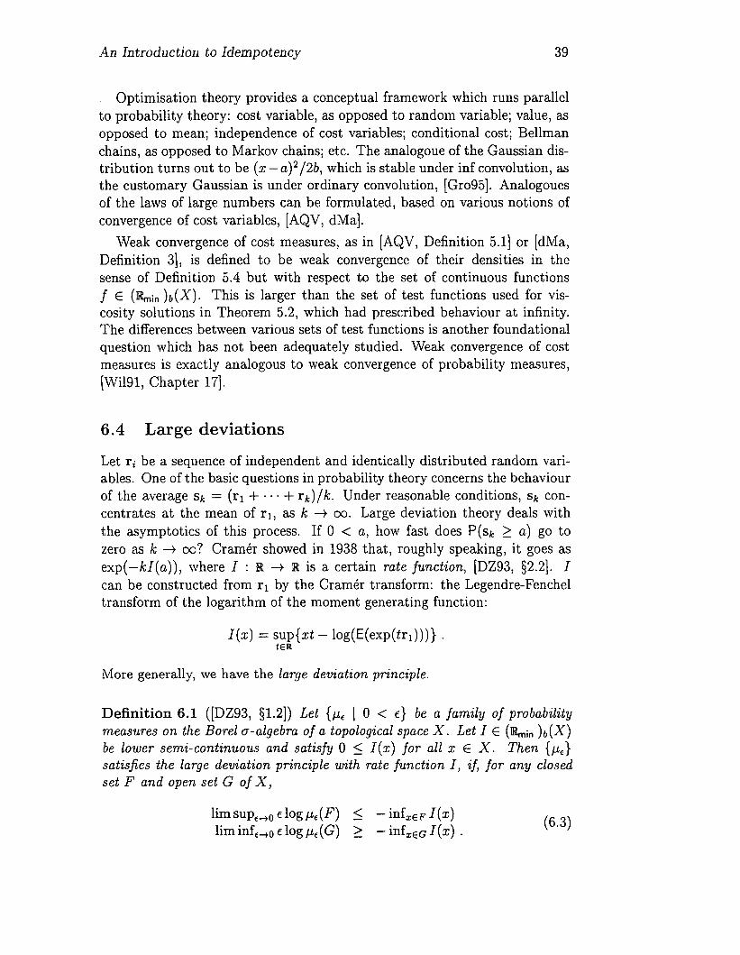
An Introduction to Idempotency 39
Optimisation theory provides a conceptual framework which runs parallelto probability theory: cost variable, as opposed to random variable; value, asopposed to mean; independence of cost variables; conditional cost; Bellmanchains, as opposed to Markov chains; etc. The analogoue of the Gaussian distribution turns out to be (x - a)2 /2b, which is stable under inf convolution, asthe customary Gaussian is under ordinary convolution, [Gro95]. Analogouesof the laws of large numbers can be formulated, based on various notions ofconvergence of cost variables, [AQV, dMa].
Weak convergence of cost measures, as in [AQV, Definition 5.1] or [dMa,Definition 3], is defined to be weak convergence of their densities in thesense of Definition 5.4 but with respect to the set of continuous functionsf E (lRmin h(X). This is larger than the set of test functions used for viscosity solutions in Theorem 5.2, which had prescribed behaviour at infinity.The differences between various sets of test functions is another foundationalquestion which has not been adequately studied. Weak convergence of costmeasures is exactly analogous to weak convergence of probability measures,[WiI91, Chapter 17].
6.4 Large deviations
Let ri be a sequence of independent and identically distributed random variables. One of the basic questions in probability theory concerns the behaviourof the average Sk = (rl + ... + rk)/k. Under reasonable conditions, Sk concentrates at the mean of rl, as k ---+ 00. Large deviation theory deals withthe asymptotics of this process. If 0 < a, how fast does P(Sk ~ a) go tozero as k ---+ oo? Cramer showed in 1938 that, roughly speaking, it goes asexp(-kI(a)), where I : lR ---+ lR is a certain rate function, [DZ93, §2.2]. Ican be constructed from rl by the Cramer transform: the Legendre-Fencheltransform of the logarithm of the moment generating function:
I(x) = sup{xt - log(E(exp(trl)))} .tER
More generally, we have the large deviation principle.
Definition 6.1 ([DZ93, §l.2]) Let {,..l£ I 0 < €} be a family of probabilitymeasures on the Borel a-algebra of a topological space X. Let I E (lRmin h(X)be lower semi-continuous and satisfy 0 ~ I(x) for all x E X. Then {tL£}satisfies the large deviation principle with rate function I, if, for any closedset F and open set G of X,
lim sUP£-tO € log tL£(F) < - infxEF I(x)lim inf£-to dog tL£(G) > - infxEG I(x) .
(6.3)

40 Jeremy Gunawardena
The papers of Akian et aI, [AQV], and del Moral, [dMa, dMSa, dMb], shedlight on the connection between large deviations and idempotency. Theorem 5.2 of [AQV] (see also [dMa]) gives a necessary and sufficient conditionfor weak convergence of measures on a metric space, which is strikingly similiar to (6.3). This suggests that the large deviation principle is a form of weakconvergence to the rate function. Proposition 6.8 of [AQV] is asserted to beequivalent to the Gartner-Ellis theorem, one of the main results of large deviation theory, [DZ93, Theorem 2.3.6]. Proposition 6.8 is analogous to the Levyconvergence theorem: weak convergence of distribution functions correspondsto pointwise convergence of characteristic functions, [Wil91, §18.1]. (Characteristic function is used here in the sense of probability theory, [WiI91, §16.1].)As in probability theory, the central limit theorem for cost variables, [AQV,Theorem 4.6] (see also [dMa]), falls out as a corollary of Proposition 6.8.
As this account suggests, the results of optimisation theory appear to encapsulate and reformulate the large deviation asymptotics of probability theory.
6.5 Topical functions and asymptotics
There is another way to approach the emergence of idempotency in the largedeviation limit. It uses the topical functions of §4.2 and formula (6.1). Wenoted in §2.9 the close analogy between the spectral theory of max-plus matrices and nonnegative matrices. This seems very similar to the analogy betweenprobability theory and optimisation theory discussed in the previous sectionbut without the large deviation mechanism for moving from the former to thelatter.
Let A E Mn(lRmax). For each 0 < h ~ 1, define the functional Eh:
Nfn(lRmax) ---t Top(n, n) by
n
(Eh(A)(Xl' ... ,xn )). := h log(L: exp((Aij + Xj)/h)) .t j=l
It is easy to check, using Lemma 4.1, that £h(A) is a topical function for allh E (0,1]. Furthermore, E1(A) = E(exp(A)), where exp(A) E Mn(lR+O
) isgiven by exp(A)ij = exp(Aij ), and E is the functional introduced in §4.2. Atthe other end, for any fixed x E lRn
, limh~o+ Eh(A)(x) = Ax, by (6.1).
We see that we have a deformation, within the space of topical functions,between E(exp(A)), representing the nonnegative matrix exp(A), and themax-plus matrix A. The class of topical functions provides us with a contextwithin which both extremes, and the intervening space, can be explored.
How do the dynamics and spectral theory of £h(A) vary with h? In particular, how do the dynamics and spectral theory of A emerge in the limit ash ---t O? Perhaps this can be viewed as a non-commutative version, appropri-

An Introduction to Idempotency 41
ate for matrices, of the problems discussed in §6.4. On this enigmatic note,we bring our survey of idempotency to a close.
References
[Aki95] M. Akian. Densities of idempotent measures and large deviations.Rapport de Recherche 2534, INRIA, April 1995.
[AQV] M. Akian, J.-P. Quadrat, and M. Viot. Duality between probability and optimization. Appears in [Gun97].
[Aub93] J.-P. Aubin. Optima and Equilibria, volume 140 of GraduateTexts in Mathematics. Springer-Verlag, 1993.
[AV93] S. Abramsky and S. Vickers. Quantales, observational logic andprocess semantics. Mathematical Structures in Computer Science,3:161-227, 1993.
[Bac94] W. Backes. The structure of longest paths in periodic graphs. PhDthesis, Universitat des Saarlandes, 1994.
[Bap95] R. Bapat. Permanents, max algebra and optimal assignment.Linear Algebra and its Applications, 226-228:73-86, 1995..
[BC93] F. Baccelli and M. Canales. Parallel simulation of stochastic Petrinets using recurrence equations. ACM Transactions on Modelingand Computer Simulation, 3:20-41, 1993.
[BCGZ84] R. E. Burkard, R. A. Cuninghame-Green, and U. Zimmermann,editors. Algebraic and Combinatorial Methods in Operations Research, volume 19 of Annals of Discrete Mathematics. NorthHolland, 1984.
[BCOQ92] F. Baccelli, G. Cohen, G. J. Olsder, and J.-P. Quadrat. Synchronization and Linearity. Wiley Series in Probability and Mathematical Statistics. John Wiley, 1992.
[BFG94] F. Baccelli, S. Foss, and B. Gaujal. Structural, temporal andstochastic properties of unbounded free-choice Petri nets. Rapport de Recherche 2411, INRIA, November 1994. To appear inIEEE Transactions on Automatic Control.
[BJ72] T. S. Blyth and M. F. Janowitz. Residuation Theory, volume102 of International Series of Monographs in Pure and AppliedMathematics. Pergammon, 1972.

42 Jeremy Gunawardena
[BM] F. Baccelli and J. Mairesse. Ergodic theorems for stochastic operators and discrete event systems. Appears in [Gun97].
[BSvdD95] R. Bapat, D. P. Stanford, and P. van den Driessche. Pattern properties and spectral inequalities in max algebra. SIAM Journal ofMatrix Analysis and Applications, 16:964-976, 1995.
[Bur90] S. M. Burns. Performance Analysis and Optimization of Asynchronous Circuits. PhD thesis, California Institute of Technology,1990.
[But94] P. Butkovic. Strong regularity of matrices-a survey of results.Discrete Applied Mathematics, 48:45-68, 1994.
[BvV92] A. Blokhuis and H. A. Wilbrink. Alternative proof of Sine's theorem on the size of a regular polygon in JRn with the £00 metric.Discrete Computational Geometry, 7:433-434, 1992.
[Car71] B. A. Carre. An algebra for network routing problems. Journalof the Institute of Mathematics and its Applications, 7:273-294,1971.
[CDQV85] G. Cohen, D. Dubois, J.-P. Quadrat, and M. Viot. A linearsystem-theoretic view of discrete-event processes and its use forperformance evaluation in manufacturing. IEEE Transactions onAutomatic Control, 30(3):210-220, 1985.
[CEL84] ~L G. Crandall, L. C. Evans, and P.-L. Lions. Some propertiesof viscosity solutions of Hamilton-Jacobi equations. Transactionsof the AMS, 282:487-502, 1984.
[CGa] D. D. Cofer and V. K. Garg. Idempotent structures in the supervisory control of discrete event systems. Appears in [Gun97].
[CGb] R. A. Cuninghame-Green. Maxpolynomials and discrete eventdynamic systems. Appears in [Gun97].
[CG62] R. A. Cuninghame-Green. Describing industrial processes withinterference and approximating their steady-state behaviour. Operational Research Quarterly, 13(1):95-100, 1962.
[CG79] R. A. Cuninghame-Green. Minimax Algebra, volume 166 of Lecture Notes in Economics and Mathematical Systems. SpringerVerlag, 1979.
[CG95] R. A. Cuninghame-Green. Minimax algebra and applications.Advances in Imaging and Electron Physics, 90:1-121, 1995.

An Introduction to Idempotency 43
[CGQ] G. Cohen, S. Gaubert, and J.-P. Quadrat. Algebraic system analysis of timed Petri nets. Appears in [Gun97].
[CIL92] M. G. Crandall, H. Ishii, and P.-L. Lions. User's guide to viscositysolutions of second order partial differential equations. Bulletinof the AMS, 27:1-67, 1992.
[CKR84] Z.-Q. Cao, K. H. Kim, and F. W. Roush. Incline Algebra andApplications. Mathematics and its Applications. Ellis-Horwood,1984.
[CMQV89] G. Cohen, P. Moller, J.-P. Quadrat, and M. Viot. Algebraictools for the performance evaluation of discrete event systems.Proceedings of the IEEE, 77(1):39-58, 1989.
[Con71] J. H. Conway. Regular Algebra and Finite Machines. Chapmanand Hall, 1971.
[CT80] M. G. Crandall and L. Tartar. Some relations between nonexpansive and order preserving maps. Proceedings of the AMS,78(3):385-390, 1980.
[DE95] J. Desel and J. Esparza. Free Choice Nets, volume 40 of Cambridge Tracts in Theoretical Computer Science. Cambridge University Press, 1995.
[DJLC53] M. L. Dubreil-Jacotin, L. Lesieur, and R. Croisot. Ler;ons surla Theorie des Treillis, des Structures Algebriques Ordonnees, etdes Treillis Geometriques. Gauthier Villars, 1953.
[dMa] P. del Moral. Maslov optimisation theory: topological aspects.Appears in [Gun97].
[dMb] P. del Moral. Maslov optimization theory: optimality versus randomness. Appears as an Appendix to [KMa].
[dMSa] P. del Moral and G. Salut. Maslov optimization theory. To appearin the Russian Journal of Mathematical Physics, 1996.
[dMSb] P. del Moral and G. Salut. Random particle methods in (max, +)optimization problems. Appears in [Gun97].
[dSa] F. d'Alessandro and J. Sakarovitch. The finite power propertyfor rational sets of the free group. Appears in [Gun97].
[DSb] P. I. Dudnikov and S. N. Samborski!. Endomorphisms of finitelygenerated free semimodules. Appears in [MS92].

44
[DZ93]
[ER95]
[ES92]
[Eva84]
[Fuc63]
[Gau]
[Gau92]
[GJM]
[GK90]
[GK95]
[GKS97]
[GMa]
[GMb]
[GM84]
Jeremy Gunawardena
A. Dembo and O. Zeitouni. Large Deviations Techniques andApplications. Jones and Bartlett, 1993.
S. Even and S. Rajsbaum. Unison, canon and sluggish clocksin networks controlled by a synchronizer. Mathematical SystemsTheory, 28:421-435, 1995.
Y. V. Egorov and M. A. Shubin, editors. Partial DifferentialEquations I, volume 30 of Encyclopaedia of Mathematical Sciences. Springer-Verlag, 1992.
1. C. Evans. Some min-max methods for the Hamilton-Jacobiequation. Indiana University Mathematics Journal, 33:31-50,1984.
L. Fuchs. Partially Ordered Algebraic Systems, volume 28 of Pureand Applied Mathematics. Pergammon, 1963.
S. Gaubert. On the Burnside problem for semigroups of matricesin the (max,+) algebra. To appear in Semigroup Forum.
S. Gaubert. Theorie des Systemes Lineaires dans les dioides. PhDthesis, L'Ecole Nationale Superieure des Mines de Paris, 1992.
B. Gaujal and A. Jean-Marie. Computational issues in recursivestochastic systems. Appears in [Gun97].
K. Goebel and W. A. Kirk. Topics in Metric Fixed Point Theory, volume 28 of Cambridge Studies in Advanced Mathematics.Cambride University Press, 1990.
J. Gunawardena and M. Keane. On the existence of cycle timesfor some nonexpansive maps. Technical Report HPL-BRIMS-95003, Hewlett-Packard Labs, 1995.
J. Gunawardena, M. Keane, and C. Sparrow. In preparation,1997.
S. Gaubert and J. Mairesse. Task resource models and (max,+)automata. Appears in [Gun97].
M. Gondran and M. Minoux. Linear algebra in dioids: a surveyof recent results. Appears in [BCGZ84].
M. Gondran and M. Minoux. Graphs and Algorithms. WileyInterscience Series in Discrete Mathematics. John Wiley, 1984.

An Introduction to Idempotency 45
[Go192] J. S. Golan. The Theory of Semirings with applications in mathematics and theoretical computer science, volume 54 of PitmanMonographs and Surveys in Pure and Applied Mathematics. Lonman Scientific and Technical, 1992.
[Gona] M. Gondran. Analyse MINMAX. To appear in C. R. Acad. Sci.Paris, 1996.
[Gonb] M. Gondran. Analyse MINPLUS. To appear in C. R. Acad. Sci.Paris, 1996.
[GPL] A. Giirel, O. C. Pastravanu, and F. L. Lewis. A system-theoreticapproach to discrete event control of manufacturing systems. Appears in [Gun97].
[Gro95] Max-Plus Working Group. Max-plus algebra and applications tosystem theory and optimal control. In Proceedings of the International Congress of Mathematicians, Zurich, 1994. Birkhauser,1995.
[Gun93] J. Gunawardena. Timing analysis of digital circuits and the theory of min-max functions. In TAU'93, ACM International Workshop on Timing Issues in the Specification and Synthesis of Digital Systems, September 1993.
[Gun94a] J. Gunawardena. Cycle times and fixed points of min-max functions. In G. Cohen and J.-P. Quadrat, editors, 11th InternationalConference on Analysis and Optimization of Systems, pages 266272. Springer LNCIS 199, 1994.
[Gun94b] J. Gunawardena. A dynamic approach to timed behaviour. InB. Jonsson and J. Parrow, editors, CONCUR'94: ConcurrencyTheory, pages 178-193. Springer LNCS 836, 1994.
[Gun94c] J. Gunawardena. Min-max functions. Discrete Event DynamicSystems, 4:377-406, 1994.
[Gun97] J. Gunawardena, editor. Idempotency. Publications of the IsaacNewton Institute. Cambridge University Press, 1997.
[GY94] P. Glasserman and D. D. Yao. Monotone Structure in DiscreteEvent Systems. Wiley Series in Probability and MathematicalStatistics. John Wiley, 1994.
[Has79] K. Hashiguchi. A decision procedure for the order of regularevents. Theoretical Computer Science, 8:69-72, 1979.

46
[Hei95]
[Ho89]
[Hop65]
[HU79]
[Joh82]
[Joh83]
[JT84]
[Kle]
[KMa]
[KMb]
[KM89]
[Kola]
[Kolb]
[Kro]
[KS86]
Jeremy Gunawardena
H. J. A. M. Heijmans. Mathematical morphology: a modernapproach in image processing based on algebra and geometry.SIAM Review, 37(1):1-36, 1995.
Y. C. Ho, editor. Special issue on Dynamics of Discrete EventSystems. Proceedings of the IEEE, 77(1), January 1989.
E. Hopf. Generalized solutions of non-linear equations of firstorder. Journal of Mathematics and Mechanics, 14:951-973, 1965.
J. E. Hopcroft and J. D. Ullman. Introduction to Automata Theory, Languages and Computation. Addison Wesley, 1979.
P. T. Johnstone. Stone Spaces, volume 3 of Studies in AdvancedMathematics. Cambridge University Press, 1982.
P. T. Johnstone. The point of pointless topology. Bulletin American Mathematical Society, 8(1):41-53, 1983.
A. Joyal and M. Tierney. An extension of the Galois theory ofGrothendieck. Memoirs of the AMS, 51(309), 1984.
S. C. Kleene. Representation of events in nerve nets and finiteautomata. Appears in [SM56].
V. N. Kolokoltsov and V. P. Maslov. Idempotent Analysis. To bepublished by Kluwer.
V. N. Kolokoltsov and V. P. Maslov. New differential equationfor the dynamics of the Pareto sets. Appears in [Gun97].
V. N. Kolokoltsov and V. P. Maslov. Idempotent analysis as atool of control theory and optimal synthesis I. Functional Analysisand Applications, 23(1):1-14, 1989.
V. N. Kolokoltsov. On linear, additive and homogeneous operators in idempotent analysis. Appears in [MS92].
V. N. Kolokoltsov. Stochastic HJB equation and WKB method.Appears in [Gun97].
D. Krob. Some automata theoretic aspects of min-max-plussemirings. Appears in [Gun97].
W. Kuich and A. Salomaa. Semirings, Automata, Languages, volume 5 of EATCS Monographs on Theoretical Computer Science.Springer-Verlag, 1986.

An Introduction to Idempotency 47
[Kui87]
[Kun72]
[Leu]
[LM]
[Mac71]
[Mas87a]
[Mas87b]
[Min88]
[MK94]
[MoI88]
[MP]
[MS]
[MS92]
[MuI86]
[Nus]
[O'B96]
W. Kuich. The Kleene and the Parikh theorem in complete semirings. In Proceedings ICALP, pages 212-225. Springer LNCS 267,1987.
J. Kuntzmann. Theorie des Reseaux. Dunod, 1972.
H. Leung. The topological approach to limitedness problem ondistance automata. Appears in [Gun97].
G. L. Litvinov and V. P. Maslov. Correspondence principle foridempotent calculus and some computer applications. Appearsin [Gun97].
S. MacLane. Categories for the Working Mathematician. Graduate Texts in Mathematics. Springer-Verlag, 1971.
V. P. Maslov. Methodes Operatorielles. Editions MIR, 1987.
V. P. Maslov. On a new principle of superposition for optimization problems. Russian Math Surveys, 42(3):43-54, 1987.
H. Mine. Nonnegative Matrices. Wiley-Interscience Series in Discrete Mathematics and Optimization. John Wiley, 1988.
V. P. Maslov and V. N. Kolokoltsov. Idempotent Analysis andits Application to Optimal Control. Nauka, Moscow, 1994. InRussian.
P. Moller. Theorie Algebrique des Systemes a Evenements Discrets. PhD thesis, Ecole des Mines de Paris, 1988.
G. Mascari and M. Pedicini. Types and dynamics in partiallyadditive categories. Appears in [Gun97].
V. P. Maslov and S. N. Samborski!. Stationary Hamilton-Jacobiand Bellman equations (existence and uniqueness of solutions).Appears in [MS92].
V. P. Maslov and S. N. Samborski!, editors. Idempotent Analysis, volume 13 of Advances in Soviet Mathematics. AmericanMathematical Society, 1992.
C. J. Mulvey. &. Rend. Circ. Mat. Palermo, 12:99-104, 1986.
R. D. Nussbaum. Periodic points of nonexpansive maps. Appearsin [Gun97].
G. L. O'Brien. Sequences of capacities, with connections to largedeviation theory. Journal of Applied Probability, 9:19-35, 1996.

48
[OR88]
[Pap91]
[Per90]
[Pin]
[Rei68]
[Rei85]
[RH80]
[Rom67]
[RS94]
[SaI73]
[Sam]
[Shu]
[Sim78]
[Sim88]
[Sin90]
Jeremy Gunawardena
G. J. Olsder and C. Roos. Cramer and Cayley-Hamilton in maxalgebra. Linear Algebra and its Applications, 101:87-108, 1988.
E. Pap. On non-addtive set functions. Atti. Sem. Mat. Fis. Univ.Modena, XXXIX:345-360, 1991.
D. Perrin. Finite automata. In J. van Leeuwen, editor, Handbookof Theoretical Computer Science Volume B, pages 1-57. Elsevier,1990.
J.-E. Pin. Tropical semirings. Appears in [Gun97].
R. Reiter. Scheduling parallel computations. Journal of the AGM,15(4):590-599, 1968.
W. Reisig. Petri Nets, volume 4 of EATGS Monographs on Theoretical Computer Science. Springer-Verlag, 1985.
C. V. Ramamoorthy and G. S. Ho. Performance evaluation ofasynchronous concurrent systems using Petri nets. IEEE Transactions on Software Engineering, SE-6(5):440-449, 1980.
1. V. Romanovskii. Optimization of stationary control of discretedeterministic process in dynamic programming. Cybernetics, 3,1967.
S. Rajsbaum and M. Sidi. On the performance of synchronizedprograms in distributed networks with random processing timesand transmission delays. IEEE Transactions on Parallel and Distributed Systems, 5:939-950, 1994.
A. Salomaa. Formal Languages. Academic Press, 1973.
S. N. Samborski!. Lagrange problem from the point of view ofidempotent analysis. Appears in [Gun97].
M. A. Shubin. Algebraic remarks on idempotent semirings andthe kernel theorem in spaces of bounded functions. Appears in[MS92].
1. Simon. Limited subsets of a free monoid. In Proceedings 19thIEEE Symposium on FOGS, pages 143-150. IEEE, 1978.
1. Simon. Recognizable sets with multiplicities in the tropicalsemiring. In Proceedings MFGS, pages 107-120. Springer LNCS324, 1988.
R. Sine. A nonlinear Perron-Frobenius theorem. Proceedings ofthe AMS, 109:331-336, 1990.

An Introduction to Idempotency 49
[SM56] C. E. Shannon and J. McCarthy, editors. Automata Studies. Annals of Mathematics Studies. Princeton University Press, 1956.
[Spa96] C. Sparrow. Existence of cycle time vectors for minmax functionsof dimension 3. Technical Report HPL-BRIMS-96-008, HewlettPackard Labs, 1996.
[SS92] T. Szymanski and N. Shenoy. Verifying clock schedules. In Digest of Technical Papers of the IEEE International Conferenceon Computer-Aided Design of Integrated Circuits, pages 124-131.IEEE Computer Society, 1992.
[ST] S. N. Samborski! and A. A. Tarashchan. The Fourier transformand semirings of Pareto sets. Appears in [MS92].
[Vic89] S. Vickers. Topology via Logic, volume 5 of Cambridge Tractsin Theoretical Computer Science. Cambridge University Press,1989.
[Vin] J. M. Vincent. Some ergodic results on stochastic iterative DEDS.To appear in Journal of Discrete Event Dynamics Systems.
[Vor67] N. N. Vorobyev. Extremal algebra of positive matrices. ElektronInformationsverarbeitung und Kybernetik, 3, 1967. In Russian.
[Wag] E. Wagneur. The geometry of finite dimensional pseudomodules.Appears in [Gun97].
[Wag91] E. Wagneur. Moduloi"ds and pseudomodules. Discrete Mathematics, 98:57-73, 1991.
[WB] E. A. Walkup and G. Borriello. A general linear max-plus solutiontechnique. Appears in [Gun97].
[Wil91] D. Williams. Probability with Martingales. Cambridge Mathematical Textbooks. Cambridge University Press, 1991.
[WXS90] C. Wende, Q. Xiangdong, and D. Shuhui. The eigen-problem andperiod analysis of the discrete event system. Systems Science andMathematical Sciences, 3:243-260, 1990.
[Zim81] U. Zimmermann. Linear and Combinatorial Optimization in Orderd Algebraic Structures, volume 10 of Annals of Discrete Mathematics. North-Holland, 1981.


![The Stratified Shortest-Paths Problem (Invited Paper)tgg22/publications/talk... · Semirings (see [Car79,GM84,GM08]) A few semirings name S ⊕, ⊗ 0 1 possible routing use sp N∞](https://static.fdocuments.us/doc/165x107/5f0c3bd57e708231d43464e4/the-stratified-shortest-paths-problem-invited-paper-tgg22publicationstalk.jpg)