An Introduction to Dynare - Boston Universitypeople.bu.edu/rking/SZGcourse/MSpresentation dynare...

Introduction to Dynare

An Introduction to Dynare1

by Michael Siemer (Boston University)

at Studienzentrum Gerzensee, SwitzerlandDoctoral Course

February, 2010

1This presentation borrows heavily from notes by M. Julliard1/35


What is Dynare?

What is Dynare?

• DYNARE: A software for the simulation and estimation of rationalexpectation models

• developed by researchers headed by M. Julliard and includingTommaso Mancini Griffoli (SZG)

• collection of functions (300+) for Matlab (other platforms alsoavailable), install routines for Windows, Mac OS, Linux (Debian,Ubuntu)

• For download at www.dynare.org free of charge

• After downloading and installation make sure to add the dynarefolder to your matlab path

2/35

www.dynare.org


What is Dynare?

What is Dynare?

• DYNARE: A software for the simulation and estimation of rationalexpectation models

• developed by researchers headed by M. Julliard and includingTommaso Mancini Griffoli (SZG)

• collection of functions (300+) for Matlab (other platforms alsoavailable), install routines for Windows, Mac OS, Linux (Debian,Ubuntu)

• For download at www.dynare.org free of charge• Dynare User Guide at http://www.dynare.org/documentation-and-support/user-guide

• Practicing Dynare athttp://homepages.nyu.edu/~ts43/research/AP_tom16.pdf,written for an earlier version of Dynare, some examples might notwork.

3/35

www.dynare.org

http://www.dynare.org/documentation-and-support/user-guide

http://www.dynare.org/documentation-and-support/user-guide

http://homepages.nyu.edu/~ts43/research/AP_tom16.pdf


What is Dynare?

’Practicing Dynare’

Provides a number of examples for Dynare. Among them are

• Cagan (1956): Demand for money during hyperinflations

• Kim and Kim (2003): International Real Business Cycle Model withComplete Markets

• Bansal and Yaron (2004): Asset pricing with risks for the long-run

4/35


Outline

Outline

1 Dynare: Introduction

2 Example I: Neoclassical Growth Model with Leisure

3 Example II: Bayesian Estimation of Example I

4 Dynare: Pros and Cons

5/35


Dynare: Introduction

Features

Features

Dynare

• solves for the steady state of DSGE model

• computes first or second order approximation of linear/nonlinearstochastic models2.→ more generally the expression for these approaches isperturbation method

• estimates DSGE models using Bayesian Maximum Likelihood

• optimal policy under commitment (Ramsey policy)

• little programming skills required (that may be a lie as we willdiscover)

2also solves deterministic models but those have become somewhat rare6/35



Features

The general problem

Et {f (yt+1yt , yt−1, ut ; θ} = 0

• where f (·) - are functions - yt is a vector of endogenous variablesthat contains both forward looking variables and predeterminedvariables, ut is a vector of exogenous shocks, θ are exogenousparameters

• E (ut) = 0, E (ut , u′t) = Σu, E (ut , u

′s) = 0 for s 6= t.

• In a stochastic framework, the unknowns are the decision functions:

yt = g(yt−1, ut) (1)

7/35



Features

First order Approximation

Equation (1) is approximated in the following way:

yt = y + Ayt−1 + But (2)

where yt = yt − y and y is steady state.

• A first order approximation is nothing else than a standard solutionthrough linearization

• A first order approximation in terms of the logarithm of the variablesprovides standard log-linearization

• Dynare uses a method proposed by Klein (2000) and Sims (2002).

• Alternative solution methods were developed e.g. King and Watson(2002), Anderson and Moore (1985)→ one difference to KW, AM is that while you have to log-linearizethe model and find the steady state yourself for those, Dynare cando it for you.

• Note: first order approximation is probably the most frequently usedmethod

8/35



Features

Second order Approximation

Equation (1) is approximated in the following way:

yt = y + Ayt−1 + But +1

2

(y ′t−1Cyt−1 + u′tDut

)+ y ′t−1Fut + GΣu (3)

• Dynare uses a method proposed by Sims(2002), Schmitt-Grohe andUribe (2003) and Collard and Julliard (2000)

• two features of second order:

1 decision rules and transition functions are 2nd order polynomials2 departure from certainty equivalence: the variance of future shocks

matters, particularly important for welfare calculation

• Note: second order approximation is being used more and more ineconomics

9/35



Features

Standard procedure if NOT using Dynare

• find model equations (FOCs, other equilibrium conditions)

• find the steady state

• identify endogenous variables, predetermined and exogenousvariables

• (log)-linearize the equations

• cast the equations in this kind of framework (this can vary slightlydepending on the method you are using):

AEtYt+1 = BYt + C0Xt + C1EtXt+1 + ....CnEtXt+n

• specify exogenous process

• write model in state space form

10/35



Features

Basics: Dynare .mod file

Can be written in Matlab and contains instructions for Dynare. Consistof four blocks

• preamble: lists variables and parameters

• model: equations of the model

• steady state or initial value: either advises Dynare to find steadystate or provides the starting point for simulations or impulseresponse functions

• shocks: defines the shocks to the system

• computation: instructs Dynare to do certain operations: simulatethe model, impulse response functions, estimate the model, etc.......

11/35



Dynare notation

Dating convention

Dynare will automatically recognize predetermined and nonpredeterminedvariables, but you must observe a few rules:

• period t variables are set during period t on the basis of the state ofthe system at period t-1 and shocks observed at the beginning ofperiod t.

• therefore, stock variables must be on an end-of-period basis:investment of period t determines the capital stock at the end ofperiod t.

• Note: Dynare 4.1 (released a few weeks ago) allows you with a newcommand to use the more conventional notation.

Let’s start with a simple example and create our own .mod file

12/35


Example I: Neoclassical Growth Model with Leisure

Model

Setup

A representative’s household problem is3

max{ct ,lt}t=00∞

E0

∞∑t=0

βt

(cθt (1− lt)1−θ)1−γ

1− γ

subject to the resource constraint

ct + it = ezt kαt l1−αt (4)

the law of motion for capital

kt+1 = it + (1− δ)kt (5)

and the stochastic process for productivity with εt ∼ N(0, 1)

zt = ρzt−1 + σεt (6)

3this example is taken from ’Practicing Dynare’ mentioned earlier13/35



Model

Equilibrium conditions

Combine (4) and (5) to get

kt+1 = ezt kα−1t lαt − ct + (1− δ)kt (7)

The Euler equation(cθt (1− lt)1−θ)1−γ

ct= βEt

[(cθt (1− lt)1−θ)1−γ

ct+1(1 + αezt+1kα−1

t+1 lαt+1 − δ)

](8)

consumption/leisure choice

1− θθ

ct

1− lt= (1− α)ezt kα−1

t lαt (9)

The equilibrium is then characterized by (6), (7), (8), (9)

14/35



Solving the Model in Dynare

The .mod file for example I

//1. Preamblevar c k lab z;varexo e;

parameters beta, theta, delta, alpha, gamma, rho, sigma;

beta = 0.987;theta = 0.357;delta = 0.012;alpha = 0.4;gamma = 2;rho = 0.95;sigma = 0.007;

15/35





//1. Preamble...

16/35





//1. Preamble...

//2. Model...

// 3. Steady state or initial value

initval; //this is either the exact steady state or an approximation anddynare then tries to find the true steady state.k = 1;c = 1;lab = 0.3;z = 0;e = 0;end;

17/35





//1. Preamble...

//2. Model...

// 3. Steady state or initial value...

// 4. Define the shocks

shocks;var e;stderr sigma;end;

18/35





// 1. Preamble// 2. Model// 3. Steady state or initial value// 4. Define the shocks// 5. Computation

steady; // finds the steady state

check; // provides the eigenvalues

stoch simul(periods=1000, irf=40, order=1); // simulates the model

dynasave (’simudata.mat’);//this is just saving the results

19/35




Now let’s switch to Matlab and run this program and see what the IRF ofan RBC model looks like.

20/35




Files produced by Dynare

Suppose our file is called example.mod. then you need to trype in matlab’dynare example’ and dynare subsequently produces a few .m files

• example.m: main Matlab script for the model

• example static.m: static model

• example dynamic.m: dynamic model

21/35




Remarks:

• there are many options you can choose for stoch simul. Check’Userguide’ p.29/30.

• be aware of what Dynare’s default settings are. For example:Moments are by default unfiltered. (and the HP filter option doesnot filter the simulated moments, only for theoretical moments)

• If some variables in the IRF do not return to their steady state, (a)check if you have enough periods in your IRF, (b) check if yourmodel is stationary (!)

• If you want to have log-linearization rather than linearization, thenyou have to change the equations somewhat. If you had before 1/cyou have to write now 1/exp(c) and the same for all other variables.

• Note that Dynare can have problems in finding the steady statedepending on the model complexity and the initial values.

22/35




New in Dynare 4.1

Ability to use conventional notation,

• before:var y, k, i;...model;k = i + (1-delta)*k(-1);...end;

• new:var y, k, i;predetermined variables k;...model;k(+1) = i + (1-delta)*k;...end;

23/35




New in Dynare 4.1

• since higher order approximation (3rd, 4th) are now sometimes beingused, Dynare 4.1 supports 3rd order approximation

• Possibility to use Anderson-Moore Algorithm to compute decisionrules

• new additions to Dynare occur every few months....

24/35


Example II: Bayesian Estimation of Example I

Estimation of DSGE Model: General

• becoming increasingly popular in economics

• more computationally intensive than calibration that we did before

• very little documentation in textbook but two options are (both inSZG library)

1 Structural Macroeconometrics by DeJong2 Methods for Applied Macroeconomic Research by Canova

• Maximum likelihood estimation and Bayesian MLE are quite related:Bayesian MLE contains an additional prior (additional information)

• A good and understandable example for MLE of DSGE models isIreland, Peter (2004): ’Technology Shocks in the New KeynesianModel’. Data and code available onhttp://www2.bc.edu/~irelandp/pro-grams.html

• Example for Estimation in ’Userguide’ does not run in Dyare4.1.........

25/35

http://www2.bc.edu/~irelandp/ pro- grams.html



Bayesian Estimation: Idea

• Uncertainty and a priori knowledge about the model and it’sparameters are described by prior probabilities

• Confrontation to the data leads to a revision of the probabilities(posterior probabilities)

• point estimates are obtained by minimizing a loss function(analogous to economic decision under uncertainty)

• testing and model comparison is done by comparing posteriorprobabilities

26/35



Estimation in Dynare

Dynare estimates the structural parameters of a model based on a linearapproximation:

Et {f (yt+1yt , yt−1, ut ; θ} = 0

Estimation steps in Dynare:

1 Computes steady state

2 linearizes the model

3 solves the linearized model

4 computes the log-likelihood via Kalman filter

5 finds the maximum of the likelihood or posterior mode

6 simulates posterior distribution with metropolis algorithm

7 computes various statistics on the basis of the posterior distribution

8 computes values of unobserved variables

9 computes forecasts and confidence intervals

27/35



Example I again

max{ct ,lt}t=00∞

E0

∞∑t=0

βt

(cθt (1− lt)1−θ)1−γ

1− γ

subject to the resource constraint

ct + it = ezt kαt l1−αt (10)

the law of motion for capital

kt+1 = it + (1− δ)kt (11)

and the stochastic process for productivity with εt ∼ N(0, σ2)

zt = ρzt−1 + εt (12)

Now, suppose we want to estimate θ, γ, ρ and the standard deviation ofε.

28/35



the .mod file

var c k lab z;varexo e;

parameters beta delta alpha rho theta gamma sigma;

beta = 0.987;delta = 0.012;alpha = 0.4;sigma = 0.007;

model;same as beforeend;

varobs c;

29/35



the .mod file cont.

initval;k = 1;c = 1;lab = 0.3;z = 0;e = 0;end;

30/35



the .mod file continued

estimated params;stderr e, inv gamma pdf, 0.95,30;rho, beta pdf,0.93,0.02;theta, normal pdf,0.3,0.05;gamma, normal pdf,2.1,0.3;end;

estimation(datafile=simudata,mh replic=1000,mh jscale=0.9,conf sig=0.9,nodiagnostic, bayesian irf);

31/35



the .mod file: Some comments

• note: you need as many shocks as you have observables

• because in this estimation Dynare updates the steady state at eachiteration, it is significantly faster to give Dynare an external steadystate file, needs to have the name: example.mod, →example steadystate.m

• for bayesian estimation we need ’priors’ and their distributions,options in Dynare are normal, gamma, beta, inverse gamma anduniform distribution.

• Where do you get the priors from? Micro estimates, existing studies,....

• Informative vs. uninformative prior

• estimation can take a LONG time (mh replic determines the numberof replications for the Metropolis Hastings algorithm, default is20000)

32/35



Let’s run this in Matlab

33/35


Dynare: Pros and Cons

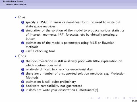
• Pros

1 specify a DSGE in linear or non-linear form, no need to write outstate space matrices

2 simulation of the solution of the model to produce various statisticsof interest: moments, IRF, forecasts, etc by virtually pressing abutton

3 estimation of the model’s parameters using MLE or Bayesianmethods

4 useful checking tool

• Cons

1 the documentation is still relatively poor with little explanation onwhich routine does what

2 relatively difficult to check for errors/mistakes3 there are a number of unsupported solution methods e.g. Projection

Methods4 estimation is still quite preliminary5 backward compatibility not guaranteed6 it does not write your dissertation (unfortunately)

34/35


Dynare: Pros and Cons

Tomorrow

• Dynare case study: Bernanke, Gertler and Gilchrist (1999): FinancialAccelerator

• how to use Dynare with a log-linear system of equations

• we will discuss the effects of financial frictions on the economy

• Why is the interesting? Financial Crisis 2008/09

35/35

An Introduction to Dynare - Boston Universitypeople.bu.edu/rking/SZGcourse/MSpresentation dynare...

Documents

Transcript of An Introduction to Dynare - Boston Universitypeople.bu.edu/rking/SZGcourse/MSpresentation dynare...