An Introduction to Dynamo: Diagrams forEvolutionary Game Dynamics∗

Francisco Franchetti and William H. Sandholm†

March 15, 2012

Abstract

Dynamo: Diagrams for Evolutionary Game Dynamics is free, open-source softwareused to create phase diagrams and other images related to dynamical systems fromevolutionary game theory. We describe how to use the software’s default settings togenerate phase diagrams quickly and easily. We then explain how to take advantageof the software’s intermediate and advanced features to create diagrams that highlightthe key properties of the dynamical system under study. Sample code and output areprovided to help demonstrate the software’s capabilities.

1. Introduction

Evolutionary game theory studies interactions among large populations of strategicallyinteracting agents. Since the introduction of the replicator dynamic by Taylor and Jonker(1978), models based on ordinary differential equations have played a central role in thisfield. Taylor and Jonker’s (1978) model, designed to provide a dynamic foundation forMaynard Smith and Price’s (1973) notion of an evolutionarily stable strategy, specifiesthat the percentage growth rate in the use of each strategy be given by the strategy’sexcess payoff—that is, by the difference between its payoff and the average payoff inthe population. This elegant model of natural selection in animal populations was thestarting point of a substantial literature that developed in mathematical biology over thenext decade, and reviewed in Hofbauer and Sigmund (1988).

By the late 1980s, economists too became interested in population dynamics for games.While their early work adhered to the biological interpretation of these dynamics as a

∗Financial support from NSF Grant SES-0851580 is gratefully acknowledged.†Department of Economics, University of Wisconsin, 1180 Observatory Drive, Madison, WI 53706,

USA. e-mail: franchetti@wisc.edu, whs@ssc.wisc.edu; websites: mywebspace.wisc.edu/franchetti/web, www.ssc.wisc.edu/˜whs.

model of natural selection in populations of preprogrammed agents, new models soonemerged in which agents were viewed as conscious decision-makers. For instance, underthe best response dynamic of Gilboa and Matsui (1991) (see also Matsui (1992) and Hof-bauer (1995b)), changes in the use of each strategy were driven not by births and deaths,but by conscious decisions to switch to the best-performing strategy.

Work in the 1990s showed that the replicator dynamic, the basic game-theoretic modelof biological natural selection, could also be provided with economic foundations. By ex-plicitly modeling the process though which individual agents decide whether and whento switch strategies, researchers showed how the replicator dynamic could be interpretedas a model of imitation among active decision makers.1 Starting from microfoundationsallowed the definition of evolutionary game dynamics based on other choice principles,from comparison to population average payoffs (Skyrms (1990), Swinkels (1993), Weibull(1996), Hofbauer (2000)), to pairwise comparisons (Sandholm (2010b)), to noisy best re-sponses (Fudenberg and Levine (1998), Hofbauer and Sandholm (2002)), to tempered bestresponses (Zusai (2011)), to best responses to samples (Oyama et al. (2012)).

In retrospect, dynamical models from the early days of game theory, particularly thework of George W. Brown, can be seen as anticipating the evolutionary game literature(Brown and von Neumann (1950)), or, in the case of fictitious play, as leading to processesintimately connected with deterministic evolutionary game dynamics (Brown (1949, 1951),Robinson (1951)). Moreover, dynamical models of behavior in traffic networks from thetransportation science literature also anticipated key aspects of the evolutionary gameapproach (Smith (1984), Nagurney and Zhang (1996)). In a complementary fashion,work by economists in evolutionary game theory turned to questions about behaviortransportation networks, and drew connections with related problems in computer science(Sandholm (2001, 2002, 2005)). Taken altogether, these research streams form the basisfor a broad interest in evolutionary game dynamics, with a wide variety of models beingsubject to intensive study.

In 2002, one of us decided to write a book to provide a unified presentation of thisburgeoning field. It soon became clear that to present evolutionary game dynamics inan informative and attractive way, it would be necessary to produce a large number ofphase diagrams and related figures, and that this could be accomplished most efficientlyby creating purpose-built software. Moreover, if the software were both publicly availableand reasonably user-friendly, it could serve as a useful research tool for the wider gametheory community. These thoughts were the origin of the Dynamo project.

Dynamo: Phase Diagrams for Evolutionary Dynamics is a collection of programs that run

1See Helbing (1992), Bjornerstedt and Weibull (1996), Weibull (1995), Hofbauer (1995a), and Schlag (1998).

–2–

within Mathematica. Although Mathematica itself is closed-source, the Dynamo code isopen-source. The current version and some legacy versions of the software are publiclyavailable on the project website, www.ssc.wisc.edu/˜whs/dynamo.

The aim of this article is to provide an introduction to Dynamo. Following a generaloverview, the article proceeds in two parts. Section 3 describes how to use Dynamoto quickly generate phase diagrams for common evolutionary dynamics and arbitrarygames, compute rest points and Nash equilibria, and perform analyses of stability. Run-ning Dynamo under its default settings is simple, and the diagrams it creates providedetailed information about the qualitative behavior of a dynamical system that might oth-erwise be difficult to obtain. In many cases, Dynamo’s default output is satisfactory foruse in publications, and many diagrams that have appeared in publication were createdin just this fashion.2

The remaining sections provide a detailed presentation of Dynamo’s features. Thesefeatures allow users to fine-tune the appearance of Dynamo output by specifying the initialconditions, durations, and appearance of solution trajectories, by selecting the functionto be presented in the background contour plot, and through the specification of variousother options. We use these features when creating our own output for publication, as thecareful selection of solution trajectories makes the qualitative properties of the dynamicseasier to perceive.

This article assumes that the reader has some background knowledge of evolutionarygame dynamics. Sandholm (2010c) is the most current treatment of this topic, as well asthe reason for Dynamo’s existence; it is also a place where many examples illustratingDynamo’s capabilities can be found.3 Although knowledge of Mathematica syntax ishelpful, most of Dynamo’s features should be accessible even to those with little or noprior experience with Mathematica.

2. Overview of Dynamo

Dynamo: Diagrams for Evolutionary Game Dynamics consists of four Mathematica note-books, corresponding to four population game environments whose phase diagramsrequire two or three dimensions. Two of the notebooks are for single-population games:Dynamo 3S.nb, for games with three strategies (and hence planar phase diagrams), andDynamo 4S.nb for games with four strategies (and hence three-dimensional phase dia-grams). The other two notebooks are for multipopulation games with two strategies for

2For a list of articles containing Dynamo output, see www.ssc.wisc.edu/˜whs/dynamo/papers.html.3A shorter and less technical introduction to evolutionary game theory is Sandholm (2009).

–3–

each population: Dynamo 2x2.nb for games with two populations (and planar phase dia-grams), and Dynamo 2x2x2.nb for games with three populations (and three-dimensionalphase diagrams).4 All of the notebooks share core code for basic numerical calculationsand make use of the same Mathematica functions; the names of common options in thedifferent notebooks are as similar as possible. But each notebook has options that arespecific to its domain.

A major goal of Dynamo is to allow researchers who use it to be able to understand andcontrol the process of creating the diagrams they need. Thus, Dynamo does not have thelook or feel of black-box software, but rather is more of a template of Mathematica code.The notebooks are presented using Mathematica’s “front end” interface, which allows forbuttons to select option values, special formatting for headers and comments, hierarchicalhiding of code, allowance of partial execution, among other convenient features. Thecurrent version of Dynamo is designed to run in Mathematica versions 6, 7, and 8, witha legacy version available for versions 4 and 5.5 Upon opening the notebooks, users ofversions 6 and 7 will receive a warning about possible incompatibilities, but these shouldbe ignored.

The Dynamo project began in 2003 with some barebones code by Bill Sandholm, theproject designer. Emin Dokumacı served as lead programmer from late 2003 through 2007,and is responsible for the legacy version of the software. The project then entered a periodof fretting over the incompatibility between Mathematica versions 5 and 6. FranciscoFranchetti became lead programmer in 2010, and updated the code for use in Mathematicaversions 6–8. Franchetti and Sandholm posted a polished version of Dynamo 3S in 2011,and testing and expansion of all four notebooks is ongoing.

3. Dynamo by default

In this section, we explain how to run the Dynamo notebooks using their defaultsettings, which can be done with a minimum of fuss. With the notebooks that createtwo-dimensional phase diagrams, 3S and 2x2, one can generate quite presentable outputwith just a few mouse clicks.

4In principle, we could create a fifth notebook for two-population games with three strategies for onepopulation and two for the other, for which the state space is a triangular prism.

5Many commands from Mathematica version 5 were eliminated entirely from version 6, so notebookswritten on either side of this divide are typically incompatible with the application on the other side.

–4–

1

2 3

Figure 1: Default Dynamo 3S output: the replicator dynamic in 123 Coordination.

3.1 Dynamo 3S

3.1.1 Running Dynamo 3S

One can generate output immediately in Dynamo 3S.nb by selecting the outermostgroup bracket (i.e., the rightmost vertical bracket) and pressing Enter or Shift-Return.After a few seconds’ delay, Dynamo creates an output notebook containing a phasediagram and supporting analysis for the default game (123 Coordination) and dynamic(the replicator dynamic). The phase diagram is presented in Figure 1.

The solution trajectories begin at a grid of initial conditions, and each solution runsfor one unit of time. The colors in the contour plot represent speeds of motion underthe dynamic: red is fast and blue is slow. (Other functions can be selected for contourplotting—see Section 4.1.2.) The black and white dots correspond to stable and unstablerest points of the dynamic.

It is easy to change which game and dynamic are analyzed. To switch to a differentnormal form game, go to the subsection called Specification of Normal Form Game,which is visible when the notebook is opened.6 There one finds a matrix A that represents

6The full location is Choice of Game → Specification of payoff parameters → Specification ofNormal Form Game.

–5–

Dynamic SourceReplicator Taylor and Jonker (1978)MSReplicator Maynard Smith (1982)ILogit[eta] Weibull (1995)

BR Gilboa and Matsui (1991)TemperedBR Zusai (2011)SampleBR[k] Oyama et al. (2012)Logit[eta] Fudenberg and Levine (1998)BNN Brown and von Neumann (1950)Smith Smith (1984)

Table 1: Built-in evolutionary dynamics in Dynamo 3S

the game to be analyzed, and whose entries can be edited directly. Alternatively, thereare buttons labeled with a number of commonly studied games; clicking one of thesebuttons will change the entries of A in the appropriate way. In the subsection Names ofStrategies, the default names of the three strategies are 1, 2, and 3; these too can bechanged directly. (One can also analyze games with nonlinear payoffs; see Section 4.2.)

To change the dynamic, scroll down to Choice of dynamic, where there are buttonscorresponding to each of the evolutionary dynamics presented in Table 1. Pressing abutton selects the dynamic by changing the value of the parameter dyn a bit further below.Three of the dynamics require parameters. To change those from their default values, goto the relevant group heading (e.g., Noise level for logit dynamics), double-click thegroup bracket to open the group, and change the parameter value therein. It is not toodifficult to define dynamics that are not built into the notebook; see footnote 17.

Once the desired settings are chosen, selecting the outermost group bracket and press-ing Enterwill generate the output notebook.

3.1.2 Dynamo 3S output

AfterEnter is pressed, Dynamo 3S.nbgenerates a new notebook labeleddynamo output 1.nbthat contains textual and graphical output. We discuss this output for the case of the repli-cator dynamic in Zeeman’s (1980) game, which can be chosen using one of the buttonsmentioned above.

The end of the notebook contains the phase diagram presented in Figure 2. In thisexample, the default phase diagram is not entirely satisfactory. We explain how to createa more appealing one by selecting individual solution trajectories in Section 4.1.1.

The first portion of the textual output concerns the game itself. In the present case

–6–

1

2 3

Figure 2: Default Dynamo 3S output: the replicator dynamic in Zeeman’s game.

it reports the normal form game under consideration, and the corresponding populationgame created by matching:

A =

0 6 -4

-3 0 5

-1 3 0

; F

x

y

x

=

6y - 4z

-3x + 5x

-x + 3y

.It then lists the Nash equilibria, and points out the equilibrium that is a regular evolution-arily stable strategy (ESS):

Nash equilibria: (1,0,0), (45, 0, 1

5), (13, 13, 13).

Regular ESS: (1,0,0).

The remainder of the textual output concerns the dynamic. First the name of thedynamic and the payoff vector field are presented:

Name of dynamic: Replicator

–7–

Law of motion: V F

x

y

z

=

x(y(6-3x-8z)+(-4+5x)z)

-y(x(3+3y-5z)+(-5+8y)z)-z(x-3y+3xy-5xz+8yz)

.Next, the rest points are analyzed for stability. In the case of a differentiable dynamic, thestability analysis is performed by linearization. Dynamo evaluates the derivative matrixof the dynamic at each rest point. If all relevant eigenvalues have negative real part(or even nonpositive real part), the rest point is categorized as stable; if at least one haspositive real part, it is categorized as unstable.7

state relevant eigenvalues relevant eigenvectors

stable: (13 ,

13 ,

13 ) −

13 +

√2

3 i, − 13 −

√2

3 i(−2+3i

√2

1−3i√

21

),(−2−3i

√2

1+3i√

21

)(1, 0, 0) −3, −1

(−110

),(−101

)unstable: (0, 0, 1) 5, −4

( 0−11

),(−101

)(0, 5

8 ,38 ) −

158 , 3

8

( 0−11

),(−651

)(0, 1, 0) 6, 3

(−110

),( 0−11

)(4

5 , 0,15 ) 4

5 , −35

(−101

),(−871

)This analysis reveals Zeeman’s (1980) well-known conclusion about his game: al-

though the Nash equilibrium (13 ,

13 ,

13 ) is not a regular ESS (or even an ESS), it is nevertheless

asymptotically stable under the replicator dynamic.

3.2 Dynamo 4S

Dynamo 4S.nb creates three-dimensional phase diagrams for four-strategy, single pop-ulation games. In Figure 3, we present a phase diagram that contains a single solutiontrajectory of the replicator dynamic in the game

A =

0 −12 0 22

20 0 0 −10−21 −4 0 3510 −2 2 0

.7The relevant eigenvalues are those corresponding to eigenvectors in the tangent space of the simplex—

see Sandholm (2010c, Section 8.5).

–8–

Figure 3: Dynamo 4S output: a chaotic attractor under the replicator dynamic.

Evidently, this solution trajectory converges to a chaotic attractor.8

The three-dimensional output leads a few important differences from Dynamo 3S.nb.Obviously, background contour plots are no longer feasible. Also, specifying a grid ofinitial conditions for solution trajectories is less satisfactory, so obtaining useful figurestypically means specifying solution trajectories one by one. We explain how this is donein Section 4.1.1.Dynamo 4S.nb takes advantage of Mathematica’s capacity to perform live rotation

of three-dimensional objects using a mouse. This makes it very useful for exploratoryanalysis of dynamics for four-strategy games, particularly in cases of chaotic dynamics,for which live rotation makes the nature of the chaotic behavior much easier to see. Liverotation also simplifies the process of finding the best viewing angles to use in figuresfor publication. On the Dynamo website, we have posted a Dynamo output notebookscontaining rotatable version of the three-dimensional figures from this article.9

8This example is due to Arneodo et al. (1980), who introduce it in the context of the Lotka-Volterraequations; also see Skyrms (1992). The attractor here is known as a Shilnikov attractor; see Hirsch et al.(2004, Chapter 16).

9See www.ssc.wisc.edu/˜whs/dynamo/3D.html. These notebooks can be opened in Mathematica 6–8,or using Wolfram’s free CDF Player; see www.wolfram.com/products/player.

–9–

D

U

L R

Figure 4: Default Dynamo 2x2 output: the Smith dynamic in 12 Coordination.

3.3 Dynamo 2x2 and 2x2x2

The remaining notebooks create phase diagrams for multipopulation games with twostrategies for each population. At present, these notebooks are less developed than thenotebooks for single-population games, but the core code for creating phase diagrams iscomplete.Dynamo 2x2.nb, for the two-population case, creates phase diagrams on a square.

Figure 4 presents the default output of this notebook for the Smith dynamic in 12 Coordi-nation. The default function of this notebook is similar to that of Dynamo 3S.nb.Dynamo 2x2x2.nb creates phase diagrams on the cube for the three-population case. As

an example, Figure 5 presents a phase diagram of the replicator dynamic in MismatchingPennies (Jordan (1993)). As in Dynamo 4S.nb, one generally needs to specify trajectoriesone by one to obtain satisfactory output.

4. Creating custom phase diagrams

We now explain the main Dynamo features used in making custom phase diagrams.We do so by means of examples, presenting both code snippets and output. Given thesimilarities among the notebooks, we focus our presentation on Dynamo 3S and 4S.

–10–

H

T

T

H

HT

Figure 5: Dynamo 2x2x2 output: the replicator dynamic in Mismatching Pennies.

4.1 Dynamo 3S

4.1.1 Trajectories

We begin with a custom phase diagram of the replicator dynamic in Zeeman’s game,presented in Figure 6. By choosing the solution trajectories carefully, the qualitativeproperties of the system are made immediately clear: we see that the connecting orbitfrom e2 = (0, 1, 0) to ( 4

5 , 0,15 ) is the separatrix between the basins of attraction of stable rest

points e1 = (1, 0, 0) and (13 ,

13 ,

13 ), and that the latter rest point is a stable spiral.

The data specifying the trajectories for the phase diagram is entered as the value of aparameter called trajectoryspecs.10 The value of this parameter is a list with entries ofthe form

{{initial condition}, time, {options}, {arrow positions}, {head lengths}}

Each such entry generates a solution starting from initial condition and running fortime units of time. Thickness, dashing, and coloring can be customized using options.If arrows are desired, the time points at which they should appear are listed in arrowpositions, and the sizes of each arrow are listed in head lengths.

10Its location is Specification of graphical output → Specifications for phase diagram →Solution trajectories.

–11–

1

2 3

Figure 6: Dynamo 3S output: the replicator dynamic in Zeeman’s game.

The trajectory data for Figure 6 is as follows:

trajectoryspecs={

{{.005,.99,.005},10,{},{1},{.03}},

{{.000454385, .994773, .00477281},10,{},{1.5},{}},

{{.00018144, .994909, .00490928},10,{},{1.75},{}},

{{.0000740367, .994963, .00496298},10,{},{2,3.5},{}},

{{.0000503846, .994975, .00497481},15,{},{2,8.2},{}},

{{.0000251918, .994987, .0049874},10,{},{2},{}},

{{.0000143953, .994993, .0049928},10,{},{2},{}},

{{.005,7/8-.0025,1/8-.0025},15,{},{1},{}},

{{.005,.75-.0025,.25-.0025},15,{},{1,10},{}},

{{.8-.02,0+.01,.2+.01},20,{},{4.6},{}},

{{113/150,1/30,16/75},20,{},{4.65},{}},

{{41/60,1/12,7/30},20,{},{3.8},{}},

{{.5-.0025,.005,.5-.0025},15,{},{1,10},{}},

{{.25-.0025,.005,.75-.0025},15,{},{.7},{}}

};

The first seven trajectories start near state e2 = (0, 1, 0), the next two start a bit to the right,

–12–

R

P S

Figure 7: Dynamo 3S output: the logit(0.08) dynamic in bad Rock-Paper-Scissors.

the following three start near ( 45 , 0,

15 ), and the final two are further toward e3. Needless

to say, some experimentation is necessary to find connecting orbits, and to achieve evenspacing. While doing so, it is best to turn off the contour plot by setting pdcontourplotto 0, since creating the contour plot generally takes up the largest share of the processingtime.11

As a second example, we present a phase diagram of the logit(.08) dynamic in the badRock-Paper-Scissors game,

A =

0 −2 11 0 −2−2 1 0

.To create this diagram, which is shown in Figure 7, we turned off the contour plot bysetting pdcontourplot to 0.

The figure reveals that this dynamic exhibits a limit cycle. While one could find a pointon the limit cycle to use as the starting point of a trajectory through experimentation, wecan use Mathematica to identify such a point automatically. We do so by means of the

11The pdcontourplot option is located in Specification of graphical output → Specificationsfor phase diagram.

–13–

following lines of code:

pointincycle={Xt1[30],Xt2[30],1-Xt1[30]-Xt2[30]}/.DEsol[{.4,.3,.3},0,30][[1]];

trajectoryspecs={

{pointincycle,10,{Thickness[.005]},{.65,1.15,1.65},{.03,.03,.03}},

{{1/3+.01,1/3-.005,1/3-.005},4.9,{Gray},{1.1,2.15,2.5},{.02,.021,.022}},

{{1,0,0},5.15,{Gray},{.5,1.5},{.03,.03}},

{{0,1,0},3.5,{Gray},{.5,1.5},{.03,.03}},

{{0,0,1},4.55,{Gray},{.5,1.5},{.03,.03}},

{{1/7,6/7,0},2,{Gray},{.5,1.8},{.03,.03}},

{{0,1/7,6/7},2,{Gray},{.5,1.8},{.03,.03}},

{{6/7,0,1/7},2,{Gray},{.5,1.8},{.03,.03}}

};

The definition of pointincycle identifies a point that is very close to the closed orbit.It calls the Dynamo function DEsol, which itself is a wrapper for Mathematica’s numericaldifferential equation solver, NDSolve. DEsol takes for granted that the relevant differentialequation is the one determined by the user’s choices of game and evolutionary dynamic.The first argument, {.4,.3,.3}, is the initial or terminal point of the solution. The nexttwo arguments, 0 and 30 are the initial and terminal times.12 The duration of 30 time unitsis enough to ensure that the solution gets very close to the limit cycle. The remaining codeextracts the desired point from the the solution trajectory.13

We use pointincycle as an initial condition in the specification of trajectories thatfollows. To emphasize the cycle, we made this trajectory thick, and made the other trajec-tories gray (instead of the default black). The second trajectory listed spirals away fromthe unstable rest point in the center of the simplex; its initial condition is a perturbation of

12Reversing the order of these times causes Dynamo to interpret {.4,.3,.3} as the terminal condition attime 30, and to compute the solution backward until time 0. Working from the terminal condition is usefulwhen trying to locate unstable cycles, or to find or trajectories that approach unstable rest points along theirstable manifolds.

13Here is a detailed explanation of what this line of code does. Dynamo’s DEsol calls upon Mathematica’sNDSolve to a the numerical solution to the differential equation. The output of NDSolve is presented asa list of so-called transformation rules. In the present case, the list contains a single transformation rule,corresponding to the lone solution of the differential equation from the initial condition provided. Thetransformation rule refers to the first two components of the solution using the functions {Xt1, Xt2}, withthe third component of the solution being defined implicitly by the fact that solutions live on the simplex.

The code /., which is the short form of Mathematica’s ReplaceAll command, has Mathematica specifythe values of the expression that precedes it by applying the transformation rule that follows it. Here{Xt1[30],Xt2[30],1-Xt1[30]-Xt2[30]}/.DEsol[{.4,.3,.3},0,30] uses /. to obtain for the time 30 posi-tion of the each solution found by DEsol. The result is a list containing a single position vector; the final[[1]] extracts the lone element from this list. It is worth noting that if this code is run in a separate cellafter initial run of Dynamo (but without the final ; that suppresses the output), Mathematica immediatelyreports the point that lies very close to the closed orbit.

–14–

the rest point itself, and did not need to be chosen very carefully. The next three trajectoriesstart at the vertices of the simplex, and the last three on repelling parts of the boundary.

4.1.2 Contour plots

The function to be presented in the contour plot is specified in Choice of contourfunction. The default setting is the Speed of motion under the dynamic, but other options,including potential functions and Lyapunov functions are provided.

Contour function output is controlled by parameters defined in Specification ofgraphical output → Specifications for phase diagram. The most important pa-rameters here are plotprecision, numberofcontours, and compressgraphic. If the val-ues of the function being plotted do not vary too quickly, then the default setting of 50, evensettings as low as 20, are adequate. On the other hand, if the function’s values changesvery quickly—as does speed under the best response dynamic in a coordination game, totake one example—then a higher setting of plotprecision, and the higher running timethat comes with it, is needed for accurate output.

Varying the choice of numberofcontours, whose default setting is 100, has obviouseffects on the figure. Settings around 50 will produce graphs that resemble topographicmaps. Settings of 150 or higher can be chosen to create the appearance of continuouschanges in color, but at the cost of higher running times and file sizes.

Finally, setting compressgraphic to 1 calls an algorithm that reduces the size of ex-ported pdf files, by using fewer and larger polygons in the construction of the contourplot. We discuss this and other points about exporting graphics in Section 5.

4.1.3 Other figures

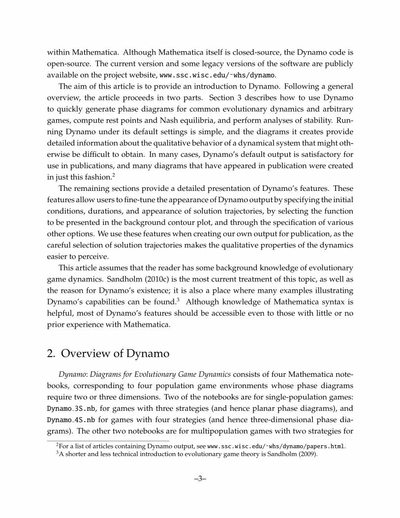
Although phase diagrams are the most commonly used Dynamo output, the softwarecan also create three other types of diagrams.14 For instance, Dynamo can produce vectorfield diagrams, which present either one or two vector fields, drawn as arrows startingfrom a grid of initial conditions in the simplex. The default vector fields used are projectedpayoffs and the dynamic itself (Figure 8).15 Dynamo can also produce three-dimensionalplots of scalar valued functions, typically the functions that appear in phase diagramsas contour plots, like speeds, potential functions, and Lyapunov functions (Figure 9).

14The options that control these diagrams are located in Specification of graphical output →Specifications for other diagrams.

15By projected payoff, we mean the orthogonal projection of the payoff vector onto the tangent spaceof the simplex. It is obtained by subtracting the unweighted average of all strategies’ payoffs from eachstrategy’s payoff—see Sandholm (2010c, Section 2.3).

–15–

1

2 3

Figure 8: Vector field diagram from Dynamo 3S: projected payoffs (blue) and the replicator dynamic (pink)in Zeeman’s game.

Finally, Dynamo can create phase diagrams that make use of a change of variable—theAkin transformation—which transports the dynamics from the simplex to a portion of thesurface of a sphere (Figure 10).16

4.2 Dynamo 4S

Drawing phase diagrams for three-dimensional dynamics introduces some new con-siderations, as one has to account for some elements of the diagram being positioned“behind” others. The next example shows how to address this issue by taking advantageof Mathematica’s capacity for rendering transparent three-dimensional objects.

Figure 11 presents a phase diagram of the replicator dynamic in a four-strategy gamewith nonlinear payoff function

Fi(x) = φ(e′iAx), where φ(π) = π3.2 and A =

1 0 1.61 .86

1.61 1 0 .860 1.61 1 .86.88 .88 .88 .87

.16This transformation is useful for studying the replicator dynamic in potential games, since under this

transformation, the replicator dynamic is the gradient system defined by the game’s potential function. SeeAkin (1979) and Sandholm et al. (2008).

–16–

Figure 9: Contour function output of Dynamo 3S for the replicator dynamic in Zeeman’s game.

1

2

3

Figure 10: Phase diagram on a portion of the sphere in Dynamo 3S: the replicator dynamic in 123Coordination. The contour plot is of a transported version of the potential function. Solutions of the

dynamic cross level sets of this function orthogonally.

–17–

The resulting differential equation can also be interpreted as a payoff functional imitativedynamic applied to the linear population game F(x) = Ax.17

To specify the nonlinear payoff function above in Dynamo, first enter the matrix A asif it were a normal form game. Then go to Choice of game → Functional form, andreplace the linear payoff definition F[x ]:=A.x;with18

f[u ]:=uˆ(3.2);

F[x ]:=f[A.x];

Figure 11 is constructed using Dynamo 4S’s default settings for coloring the faces ofthe simplex, which cause them to be rendered in a moderately transparent light green.Both the color and the opacity of the individual faces are easy to adjust.19 The solutiontrajectories in the phase diagram were specified using the following code:

pointincycle={Xt1[30],Xt2[30],Xt3[30],1-Xt1[30]-Xt2[30]-Xt3[30]}/.

DEsol[{3/4,1/8,1/8,0},0,30][[1]];

trajectoryspecs={

{pointincycle,6.85,{Black,Thickness[.0075],Opacity[.8]},{.7,4,5.6},},

{.03,.03,.03}},

{{1/4,3/8+.05,3/8-.05,0},18.5,{Gray,Thickness[.005],Opacity[.3]},

{.55,4.5,9,15,18.5},{.025,.025,.025,.025,.025}},

{{.05,.05,.9,0},9,{Gray,Thickness[.005],Opacity[.3]},{.6,3.8,6.5,8.6},

{.025,.025,.025,.025}},

{{1/3-.05,1/3-.05,1/3-.05,.15},200,{Black,Thickness[.005],Opacity[.3]},{200},},

{.025}},

{{1/3-.02999,1/3-.030005,1/3-.030005,.09},102,{Blue,Thickness[.005],Opacity[.7]},

{20,87,90,94.4,102},{.025,.025,.025,.025,.025}},

{{.15,.025,.025,.8},55,{Red,Thickness[.005],Opacity[.3]},{20,30,39,43,46.5,55},

{.025,.025,.025,.025,.025,.025}}

};

17See Hofbauer and Weibull (1996), as well as Viossat (2011), from which this example is taken. It followsthat one could have obtained the same differential equation by defining the appropriate payoff functionalimitative dynamic in Dynamo, and then applying it to F(x) = Ax. Defining new dynamics is not difficult,but takes a few steps to accomplish. The definitions of the built-in dynamics are presented in Choice ofdynamic → Definitions of dynamics; these can be used as a template for defining a new dynamic underthe heading Other.

18This definition works because of a quirk in Mathematica’s syntax: when a function that takes a scalarargument is applied to a vector, the function is evaluated separately on each component of the vector.

19The relevant parameters can be found in Specification of graphical output → Specificationsfor phase diagram → Face shading and viewpoint.

–18–

Figure 11: Dynamo 4S output: the replicator dynamic in Viossat’s (2011) game.

Apart from the obvious adjustments needed for the four-strategy setting, the mainnovelties here are the use of Mathematica’s Opacity option to specify how transparenteach solution looks, and use of colors to distinguish the solutions. For the latter, onecan also call Dynamo 4S’s option "rainbow" to obtain solutions whose colors vary overtime, as we did in Figure 3. Finally, we disabled the drawing of dots by setting thedrawnashequilibria and drawrestpoints options to 0.20

5. Creating output files for publication

A main purpose of Dynamo is to create figures for publication. There are a varietyof methods for creating output files of plots created in Mathematica, and the results oneobtains can vary substantially with the method used. Our recommendations for howto proceed depend on the nature of the graphic, on whether the graphic will undergopost-processing, and on the platform in which Mathematica is being used.21

For two-dimensional graphics, let us first reiterate that for diagrams with contour

20These parameters are located in Specification of graphical output → Specifications for

phase diagram → Drawing dots at rest points and Nash equilibria.21An excellent source of information on working with Mathematica graphics, including the creation

of files for publication, is a website maintained by Jens Nockel: see pages.uoregon.edu/noeckel/MathematicaGraphics.html.

–19–

plots, one should set compressgraphic to 1 before creating the final version of the figureif file size is of any concern.22 However, as this option slows the program down quitesubstantially, it should not be used until the final version of the figure is ready.

One can create pdf output by clicking on the graphic, go to File → Save SelectionAs, and choosing the PDF file format. Mac users can also generate quality pdfs withconsiderably smaller file sizes by going to File → Print Selection, and then selectingSave as Adobe PDF.

In some cases one needs to perform post-processing of Dynamo output using a vectorgraphics editor (like Adobe Illustrator). For instance, one might want to add a roundedrectangle to represent a component of rest points.23 To accomplish this, one needs toexport the graphic in eps format: go to File → Save Selection As and select EPS.

When working with three-dimensional graphics, we recommend using Mathematica’spdf exporting engine to create a bitmapped pdf. Click on the graphic and go to File→ Save Selection As. In the window that appears, make sure the file format is PDF;then select Options..., and then Use Bitmap Representation. For the RasterizationResolution, choose Custom. We find that a setting of 1200 dpi gives very high qualityphase diagrams, while a setting of 600 dpi is enough for graphs like Figure 9.24 Be warnedthat bitmapped images with high resolutions may take a few minutes to create.

As we noted earlier, one of Mathematica’s more impressive features is its ability tolet one rotate three dimensional images using a mouse. Therefore, one need only run anotebook once to be able to look at and export a graphic from multiple points of viewafter running the notebook. Still, looking at a graphic from a few vantage point is nota full substitute for rotating the image oneself. We therefore encourage the posting ofDynamo output notebooks as online appendices, so that readers can enjoy this experiencefor themselves.

6. Numerical methods behind Dynamo

We now offer some brief remarks on the numerical methods used in Dynamo, andmention some of the problems that these methods occasionally create.

22This option is found in Specification of graphical output → Specifications for phase

diagram.23See Sandholm (2010c, Figure 5.7).24Mac users who work in TeXShop will find that bitmap figures appearing in pdfs look ugly in TeXShop’s

pdf viewer. Fortunately, the figures will look just fine when the pdf is opened in any standard viewer.

–20–

6.1 Solving nonlinear ordinary differential equations

Generally speaking, nonlinear ordinary differential equations (ODEs) in two or moredimensions do not admit closed-form solutions. Therefore, the diagrams created byDynamo are based on numerical solutions created using Mathematica’s sophisticatednumerical ODE solver. In the case of the replicator dynamic, these methods tend to workquite well, and we have rarely experienced problems. The difficulties we do encountertend to arise when we work with dynamics that change speed rapidly, and the troubleusually occurs near rest points. Fortunately these problems do not occur too often, andare generally easy to spot—for instance, a solution trajectory may suddenly jump out ofthe state space. Users are welcome to contact us for suggestions should such problemsarise.

A variety of algorithms exist for obtaining numerical solutions to ODEs.25 Mathe-matica’s numerical ODE solver, called using the command NDSolve, uses a closed-sourceadaptive algorithm to select and switch among the basic algorithms.26 However, thesolver also allows one to select a particular algorithm to employ. In Dynamo, one cantake advantage of this possibility by altering the definition of the DESol function, whichis called whenever a solution must be found.27

6.2 Finding rest points and Nash equilibria

For many of the evolutionary dynamics considered in the literature, there are resultsthat characterize the dynamics’ rest points directly in terms of the payoffs of the underlyinggame. For instance, the rest points of the replicator dynamic and other imitative dynamicsare the restricted equilibria of the underlying game—that is, the states at which all strategiesin use receive the same payoff. If this common payoff at least as large as that of any unusedstrategy, then the state is a Nash equilibrium. Furthermore, for many dynamics based ondirect evaluation of strategies, including the best response, BNN, and Smith dynamics,rest points and Nash equilibria are identical.28 In all of these cases, one can find rest pointswithout having to work directly with nonlinear ODEs, but by instead directly analyzingthe game in question.

Dynamo finds restricted equilibria and Nash equilibria of linear games using a pro-cedure that is exact in generic cases—namely, those in which the number of equilibria

25See, for example, Press et al. (2007).26See reference.wolfram.com/mathematica/tutorial/NDSolveOverview.html.27See the Dynamo notebooks for documentation. Dynamo takes advantage of this property when finding

solutions to the projection dynamic (Nagurney and Zhang (1996); Lahkar and Sandholm (2008)), whichseems to proceed most smoothly using the Runge-Kutta-Fehlberg method of orders 5 and 4.

28See Sandholm (2010c, Chapters 4–6).

–21–

is finite. The procedure divides the state space into regions corresponding to differentsupports, and then uses Mathematica’s Solve function to locate the restricted equilibria ineach region. Once the set of restricted equilibria is determined, the set of Nash equilibriais easily obtained by checking the additional condition on payoffs to unused strategies.

To find the rest points of other dynamics, and when working with games with non-linear payoffs, Dynamo finds rest points, restricted equilibria, and Nash equilibria usingnumerical methods. It starts by specifying a grid of points in the simplex. At each of thesepoints, it uses Mathematica’s FindRoot command to attempt to find a nearby rest pointor restricted equilibrium.29 This approach works well in cases where the number of restpoints is finite, but is slower than the exact routine described above.

We should emphasize that Dynamo makes no attempt to find connected components ofrest points or equilibria. When these exist, Dynamo will find a random selection of pointsin the component. In such cases, creating a phase diagram that displays the componentcorrectly is accomplished most easily through post-processing (see Section 5).

6.3 Determining stability of rest points

Dynamo uses a number of different methods to determine stability of rest points.For differentiable dynamics, in particular the replicator and logit dynamics, Dynamodetermines stability using linearization, which yields the correct categorization so long asthe rest point is hyperbolic.30 Moreover, because regular ESSs are locally stable under thebasic evolutionary dynamics, Dynamo uses this criterion to evaluate stability wheneverit applies.31

When these exact methods fail, Dynamo uses a rough test to evaluate stability. Theprogram randomly chooses several initial conditions in a neighborhood of the rest point,computes solutions originating at these initial conditions, then evaluates whether thesesolutions remain close to the rest point. If all of them do, the rest point is categorizedas stable; if not, it is categorized as unstable. Clearly, this procedure is sensitive to theparameters used to define the test, and mistaken categorizations are not unusual.32 Thus,apart from the cases described in the previous paragraph, Dynamo’s classifications are

29By default, FindRoot employs Newton’s method, but other methods are available and can be selectedmanually. See reference.wolfram.com/mathematica/ref/FindRoot.html.

30For more on linearization of game dynamics, see Sandholm (2010c, Sections 8.5, 8.6, and 8.C).31For more on local stabilty of ESSs, see Hofbauer and Sigmund (1988), Cressman (1997), Sandholm

(2010a), and Sandholm (2010c, Sections 8.3 and 8.4).32If a certain class of examples systematically causes problems, one can tune the parameters of the test to

obtain better performance. The relevant parameters are located in Specification of graphical output→ Specifications for phase diagram → Tuning stability tests.

–22–

only intended as educated guesses, and the coloring of dots in phase diagrams should notbe taken as definitive indications of stability or instability.

7. Conclusion

Dynamo: Diagrams for Evolutionary Game Dynamics is free, open-source software de-signed for use by researchers and students working with evolutionary game dynamics.We encourage its use both for exploratory analysis and for the creation of figures forpublication, both of which can be accomplished with surprisingly little effort. This paperexplains how to use Dynamo with its default settings, and how to take advantage of avariety of its other features. But there are many further features that we did not explain;these can be found by exploring the Dynamo notebooks, where further documentationcan also be found. Dynamo is a continuing project, and we encourage users to contact uswith questions and feedback about the software.

References

Akin, E. (1979). The Geometry of Population Genetics. Springer, Berlin.

Arneodo, A., Coullet, P., and Tresser, C. (1980). Occurrence of strange attractors in three-dimensional Volterra equations. Physics Letters, 79A:259–263.

Bjornerstedt, J. and Weibull, J. W. (1996). Nash equilibrium and evolution by imitation. InArrow, K. J. et al., editors, The Rational Foundations of Economic Behavior, pages 155–181.St. Martin’s Press, New York.

Brown, G. W. (1949). Some notes on computation of games solutions. Report P-78, TheRand Corporation.

Brown, G. W. (1951). Iterative solutions of games by fictitious play. In Koopmans, T. C.et al., editors, Activity Analysis of Production and Allocation, pages 374–376. Wiley, NewYork.

Brown, G. W. and von Neumann, J. (1950). Solutions of games by differential equations. InKuhn, H. W. and Tucker, A. W., editors, Contributions to the Theory of Games I, volume 24of Annals of Mathematics Studies, pages 73–79. Princeton University Press, Princeton.

Cressman, R. (1997). Local stability of smooth selection dynamics for normal form games.Mathematical Social Sciences, 34:1–19.

–23–

Fudenberg, D. and Levine, D. K. (1998). The Theory of Learning in Games. MIT Press,Cambridge.

Gilboa, I. and Matsui, A. (1991). Social stability and equilibrium. Econometrica, 59:859–867.

Helbing, D. (1992). A mathematical model for behavioral changes by pair interactions. InHaag, G., Mueller, U., and Troitzsch, K. G., editors, Economic Evolution and DemographicChange: Formal Models in Social Sciences, pages 330–348. Springer, Berlin.

Hirsch, M. W., Smale, S., and Devaney, R. L. (2004). Differential Equations, DynamicalSystems, and an Introduction to Chaos. Elsevier, Amsterdam.

Hofbauer, J. (1995a). Imitation dynamics for games. Unpublished manuscript, Universityof Vienna.

Hofbauer, J. (1995b). Stability for the best response dynamics. Unpublished manuscript,University of Vienna.

Hofbauer, J. (2000). From Nash and Brown to Maynard Smith: Equilibria, dynamics, andESS. Selection, 1:81–88.

Hofbauer, J. and Sandholm, W. H. (2002). On the global convergence of stochastic fictitiousplay. Econometrica, 70:2265–2294.

Hofbauer, J. and Sigmund, K. (1988). Theory of Evolution and Dynamical Systems. CambridgeUniversity Press, Cambridge.

Hofbauer, J. and Weibull, J. W. (1996). Evolutionary selection against dominated strategies.Journal of Economic Theory, 71:558–573.

Jordan, J. S. (1993). Three problems in learning mixed-strategy Nash equilibria. Games andEconomic Behavior, 5:368–386.

Lahkar, R. and Sandholm, W. H. (2008). The projection dynamic and the geometry ofpopulation games. Games and Economic Behavior, 64:565–590.

Matsui, A. (1992). Best response dynamics and socially stable strategies. Journal of EconomicTheory, 57:343–362.

Maynard Smith, J. (1982). Evolution and the Theory of Games. Cambridge University Press,Cambridge.

Maynard Smith, J. and Price, G. R. (1973). The logic of animal conflict. Nature, 246:15–18.

Nagurney, A. and Zhang, D. (1996). Projected Dynamical Systems and Variational Inequalitieswith Applications. Kluwer, Dordrecht.

Oyama, D., Sandholm, W. H., and Tercieux, O. (2012). Sampling best response dynamicsand deterministic equilibrium selection. Unpublished manuscript, University of Tokyo,University of Wisconsin, and Paris School of Economics.

–24–

Press, W. H., Teukolsky, S. A., Vetterling, W. T., and Flannery, B. P. (2007). NumericalRecipes: The Art of Scientific Computing. Cambridge University Press, Cambridge, thirdedition.

Robinson, J. (1951). An iterative method of solving a game. Annals of Mathematics, 54:296–301.

Sandholm, W. H. (2001). Potential games with continuous player sets. Journal of EconomicTheory, 97:81–108.

Sandholm, W. H. (2002). Evolutionary implementation and congestion pricing. Review ofEconomic Studies, 69:667–689.

Sandholm, W. H. (2005). Negative externalities and evolutionary implementation. Reviewof Economic Studies, 72:885–915.

Sandholm, W. H. (2009). Evolutionary game theory. In Meyers, R. A., editor, Encyclopediaof Complexity and Systems Science, pages 3176–3205. Springer, Heidelberg.

Sandholm, W. H. (2010a). Local stability under evolutionary game dynamics. TheoreticalEconomics, 5:27–50.

Sandholm, W. H. (2010b). Pairwise comparison dynamics and evolutionary foundationsfor Nash equilibrium. Games, 1:3–17.

Sandholm, W. H. (2010c). Population Games and Evolutionary Dynamics. MIT Press, Cam-bridge.

Sandholm, W. H., Dokumacı, E., and Franchetti, F. (2012). Dynamo: Diagrams for evolu-tionary game dynamics. Software. http://www.ssc.wisc.edu/∼whs/dynamo.

Sandholm, W. H., Dokumacı, E., and Lahkar, R. (2008). The projection dynamic and thereplicator dynamic. Games and Economic Behavior, 64:666–683.

Schlag, K. H. (1998). Why imitate, and if so, how? A boundedly rational approach tomulti-armed bandits. Journal of Economic Theory, 78:130–156.

Skyrms, B. (1990). The Dynamics of Rational Deliberation. Harvard University Press, Cam-bridge.

Skyrms, B. (1992). Chaos in game dynamics. Journal of Logic, Language, and Information,1:111–130.

Smith, M. J. (1984). The stability of a dynamic model of traffic assignment—an applicationof a method of Lyapunov. Transportation Science, 18:245–252.

Swinkels, J. M. (1993). Adjustment dynamics and rational play in games. Games andEconomic Behavior, 5:455–484.

–25–

Taylor, P. D. and Jonker, L. (1978). Evolutionarily stable strategies and game dynamics.Mathematical Biosciences, 40:145–156.

Viossat, Y. (2011). Monotonic dynamics and dominated strategies. Unpublishedmanuscript, Universite Paris-Dauphine.

Weibull, J. W. (1995). Evolutionary Game Theory. MIT Press, Cambridge.

Weibull, J. W. (1996). The mass action interpretation. Excerpt from ’The work of JohnNash in game theory: Nobel Seminar, December 8, 1994’. Journal of Economic Theory,69:165–171.

Zeeman, E. C. (1980). Population dynamics from game theory. In Nitecki, Z. and Robinson,C., editors, Global Theory of Dynamical Systems (Evanston, 1979), number 819 in LectureNotes in Mathematics, pages 472–497, Berlin. Springer.

Zusai, D. (2011). The tempered best response dynamic. Unpublished manuscript, Uni-versity of Wisconsin.

–26–