An introduction to (co)algebra and (co)induction - CWIjanr/papers/files-of-papers/2011_Jacobs... ·...

1

An introduction to (co)algebra and (co)induction

1.1 Introduction

Algebra is a well-established part of mathematics, dealing with sets with oper-ations satisfying certain properties, like groups, rings , vector spaces, etcetera.Its results are essential throughout mathematics and other sciences. Universalalgebra is a part of algebra in which algebraic structures are studied at a highlevel of abstraction and in which general notions like homomorphism, subalge-bra, congruence are studied in themselves, see e.g. [Coh81, MT92, Wec92]. Afurther step up the abstraction ladder is taken when one studies algebra withthe notions and tools from category theory. This approach leads to a particu-larly concise notion of what is an algebra (for a functor or for a monad), see forexample [Man74]. The conceptual world that we are about to enter owes muchto this categorical view, but it also takes inspiration from universal algebra, seee.g. [Rut00].

In general terms, a program in some programming language manipulates data.During the development of computer science over the past few decades it becameclear that an abstract description of these data is desirable, for example to ensurethat one’s program does not depend on the particular representation of the dataon which it operates. Also, such abstractness facilitates correctness proofs. Thisdesire led to the use of algebraic methods in computer science, in a branchcalled algebraic specification or abstract data type theory . The object of studyare data types in themselves, using notions and techniques which are familiarfrom algebra. The data types used by computer scientists are often generatedfrom a given collection of (constructor) operations. The same applies in factto programs, which themselves can be viewed as data too. It is for this reasonthat “initiality” of algebras plays such an important role in computer science (asfirst clearly emphasised in [GTW78]). See for example [EM85, Wir90, Wec92]for more information.

1

2 1 An introduction to (co)algebra and (co)induction

Standard algebraic techniques have proved useful in capturing various essen-tial aspects of data structures used in computer science. But it turned out to bedifficult to algebraically describe some of the inherently dynamical structuresoccuring in computing. Such structures usually involve a notion of state, whichcan be transformed in various ways. Formal approaches to such state-baseddynamical systems generally make use of automata or transition systems, seee.g. [Plo81, Par81, Mil89] as classical early references. During the last decadethe insight gradually grew that such state-based systems should not be describedas algebras, but as so-called coalgebras. These are the formal duals of algebras,in a way which will be made precise in this tutorial. The dual property of ini-tiality for algebras, namely finality, turned out to be crucial for such coalgebras.And the logical reasoning principle that is needed for such final coalgebras isnot induction but coinduction.

These notions of coalgebra and coinduction are still relatively unfamiliar, andit is our aim in this tutorial to explain them in elementary terms. Most of theliterature already assumes some form of familiarity either with category theory,or with the (dual) coalgebraic way of thinking (or both).

Before we start, we should emphasise that there is no new (research) materialin this tutorial. Everything that we present is either known in the literature,or in the folklore, so we do not have any claims to originality. Also, our mainconcern is with conveying ideas, and not with giving a correct representation ofthe historical developments of these ideas. References are given mainly in orderto provide sources for more (background) information.

Also, we should emphasise that we do not assume any knowledge of categorytheory on the part of the reader. We shall often use the diagrammatic notationwhich is typical of category theory, but only in order to express equality of twocomposites of functions, as often used also in other contexts. This is simplythe most efficient and most informative way of presenting such information.But in order to fully appreciate the underlying duality between algebra andinduction on the one hand, and coalgebra and coinduction on the other, someelementary notions from category theory are needed, especially the notions offunctor (homomorphism of categories), and of initial and final (also called ter-minal) object in a category. Here we shall explain these notions in the concreteset-theoretic setting in which we are working, but we definitely encourage theinterested reader who wishes to further pursue the topic of this tutorial to studycategory theory in greater detail. Among the many available texts on categorytheory, [Pie91, Wal91, AM75, Awo06] are recommended as easy-going startingpoints, [BW90, Cro93, LS86] as more substantial texts, and [Lan71, Bor94] asadvanced reference texts.

1.1 Introduction 3

This tutorial starts with some introductory expositions in Sections 1.2 – 1.4.The technical material in the subsequent sections is organised as follows.

(1) The starting point is ordinary induction, both as a definition principleand as a proof principle. We shall assume that the reader is familiarwith induction, over natural numbers, but also over other data types,say of lists, trees or (in general) of terms. The first real step is to refor-mulate ordinary induction in a more abstract way, using initiality (seeSection 1.5). More precisely, using initiality for “algebras of a functor”.This is something which we do not assume to be familiar. We thereforeexplain how signatures of operations give rise to certain functors, andhow algebras of these functors correspond to algebras (or models) of thesignatures (consisting of a set equipped with certain functions interpret-ing the operations). This description of induction in terms of algebras(of functors) has the advantage that it is highly generic, in the sense thatit applies in the same way to all kinds of (algebraic) data types. Further,it can be dualised easily, thus giving rise to the theory of coalgebras.

(2) The dual notion of an algebra (of a functor) is a coalgebra (of a functor).It can also be understood as a model consisting of a set with certainoperations, but the direction of these operations is not as in algebra. Thedual notion of initiality is finality, and this finality gives us coinduction,both as a definition principle and as a reasoning principle. This patternis as in the previous point, and is explained in Section 1.6.

(3) In Section 1.7 we give an alternative formulation of the coinductive rea-soning principle (introduced in terms of finality) which makes use ofbisimulations. These are relations on coalgebras which are suitably closedunder the (coalgebraic) operations; they may be understood as duals ofcongruences, which are relations which are closed under algebraic oper-ations. Bisimulation arguments are used to prove the equality of twoelements of a final coalgebra, and require that these elements are in abisimulation relation.

(4) In Section 1.8 we present a coalgebraic account of transition systems and asimple calculus of processes. The latter will be defined as the elements of afinal coalgebra. An elementary language for the construction of processeswill be introduced and its semantics will be defined coinductively. As weshall see, this will involve the mixed occurrence of both algebraic andcoalgebraic structures. The combination of algebra and coalgebra willalso play a central role in Section 1.9, where a coalgebraic description isgiven of trace semantics.

In a first approximation, the duality between induction and coinduction that


we intend to describe can be understood as the duality between least and great-est fixed points (of a monotone function), see Exercise 1.10.3. These notionsgeneralise to least and greatest fixed points of a functor, which are suitablydescribed as initial algebras and final coalgebras. The point of view mentionedin (1) and (2) above can be made more explicit as follows—without going intotechnicalities yet. The abstract reformulation of induction that we will describeis:

induction = use of initiality for algebras

An algebra (of a certain kind) is initial if for an arbitrary algebra (of the samekind) there is a unique homomorphism (structure-preserving mapping) of alge-bras: (

initialalgebra

)//_________ unique

homomorphism

(arbitraryalgebra

)(1.1)

This principle is extremely useful. Once we know that a certain algebra isinitial, by this principle we can define functions acting on this algebra. Initialityinvolves unique existence, which has two aspects:

Existence. This corresponds to (ordinary) definition by induction.

Uniqueness. This corresponds to proof by induction. In such uniquenessproofs, one shows that two functions acting on an initial algebra are the sameby showing that they are both homomorphisms (to the same algebra).

The details of this abstract reformulation will be elaborated as we proceed.Dually, coinduction may be described as:

coinduction = use of finality for coalgebras

A coalgebra (of some kind) is final if for an arbitrary coalgebra (of the samekind), there is a unique homomorphism of coalgebras as shown:(

arbitrarycoalgebra

)unique

homomorphism//_________(

finalcoalgebra

)(1.2)

Again we have the same two aspects: existence and uniqueness, correspondingthis time to definition and proof by coinduction.

The initial algebras and final coalgebras which play such a prominent rolein this theory can be described in a canonical way: an initial algebra can beobtained from the closed terms (i.e. from those terms which are generated byiteratively applying the algebra’s constructor operations), and the final coalge-bra can be obtained from the pure observations. The latter is probably not veryfamiliar, and will be illustrated in several examples in Section 1.2.

1.2 Algebraic and coalgebraic phenomena 5

History of this chapter: An earlier version of this chapter was publishedas “A Tutorial on (Co)(Algebras and (Co)Induction”, in: EATCS Bulletin 62(1997), p.222–259. More then ten years later, the present version has beenupdated. Notably, two sections have been added that are particularly relevantfor the context of the present book: Processes coalgebraically (Section 1.8), and:Trace semantics coalgebraically (Section 1.9). In both these sections both initialalgebras and final coalgebras arise in a natural combination. In addition, thereferences to related work have been brought up-to-date.

Coalgebra has by now become a well-established part of the foundations ofcomputer science and (modal) logic. In the last decade, much new coalge-braic theory has been developed, such as so-called universal coalgebra [Rut00,Gum99], in analogy to universal algebra, and coalgebraic logic, generalising invarious ways classical modal logic, see for instance [Kur01, Kur06, CP07, Kli07]for an overview. But there is much more, none of which is addressed in anydetail here. Much relevant recent work and many references can be found in theproceedings of the workshop series CMCS: Coalgebraic Methods in ComputerScience (published in the ENTCS series) and CALCO: Conference on Algebraand Coalgebra in Computer Science (published in the LNCS series). The aimof this tutorial is in essence still the same as it was ten years ago: to provide abrief introduction to the field of coalgebra.

1.2 Algebraic and coalgebraic phenomena

The distinction between algebra and coalgebra pervades computer science andhas been recognised by many people in many situations, usually in terms ofdata versus machines. A modern, mathematically precise way to express thedifference is in terms of algebras and coalgebras. The basic dichotomy maybe described as construction versus observation. It may be found in processtheory [Mil89], data type theory [GGM76, GM82, AM82, Kam83] (includingthe theory of classes and objects in object-oriented programming [Rei95, HP95,Jac96b, Jac96a]), semantics of programming languages [MA86] (denotationalversus operational [RT94, Tur96, BV96]) and of lambda-calculi [Pit94, Pit96,Fio96, HL95], automata theory [Par81], system theory [Rut00], natural languagetheory [BM96, Rou96] and many other fields.

We assume that the reader is familiar with definitions and proofs by (ordinary)induction. As a typical example, consider for a fixed data set A, the set A? =list(A) of finite sequences (lists) of elements of A. One can inductively define alength function len:A? → N by the two clauses:

len(〈〉) = 0 and len(a · σ) = 1 + len(σ)


for all a ∈ A and σ ∈ A?. Here we have used the notation 〈〉 ∈ A? for theempty list (sometimes called nil), and a ·σ (sometimes written as cons(a, σ)) forthe list obtained from σ ∈ A? by prefixing a ∈ A. As we shall see later, thedefinition of this length function len:A? → N can be seen as an instance of theabove initiality diagram (1.1).

A typical induction proof that a predicate P ⊆ A? holds for all lists requiresus to prove the induction assumptions

P (〈〉) and P (σ)⇒ P (a · σ)

for all a ∈ A and σ ∈ A?. For example, in this way one can prove that len(σ ·a) =1 + len(σ) by taking P = {σ ∈ A? | ∀a ∈ A. len(σ ·a) = 1 + len(σ)}. Essentially,this induction proof method says that A? has no proper subalgebras. In this(algebraic) setting we make use of the fact that all finite lists of elements of Acan be constructed from the two operations nil ∈ A? and cons:A × A? → A?.As above, we also write 〈〉 for nil and a · σ for cons(a, σ).

Next we describe some typically coalgebraic phenomena, by sketching somerelevant examples. Many of the issues that come up during the description ofthese examples will be explained in further detail in later sections.

(i) Consider a black-box machine (or process) with one (external) buttonand one light. The machine performs a certain action only if the button ispressed. And the light goes on only if the machine stops operating (i.e. hasreached a final state); in that case, pressing the button has no effect any more.A client on the outside of such a machine cannot directly observe the internalstate of the machine, but (s)he can only observe its behaviour via the button andthe light. In this simple (but paradigmatic) situation, all that can be observeddirectly about a particular state of the machine is whether the light is on ornot. But a user may iterate this experiment, and record the observations aftera change of state caused by pressing the button1. In this situation, a user canobserve how many times (s)he has to press the button to make the light go on.This may be zero times (if the light is already on), n ∈ N times, or infinitelymany times (if the machine keeps on operating and the light never goes on).

Mathematically, we can describe such a machine in terms of a set X, whichwe understand as the unknown state space of the machine, on which we have afunction

button:X // {∗} ∪X

where ∗ is a new symbol not occurring in X. In a particular state s ∈ X, apply-

1 It is assumed that such actions of pressing a button happen instantaneously, so that there is alwaysan order in the occurrence of such actions.


ing the function button—which corresponds to pressing the button—has two pos-sible outcomes: either button(s) = ∗, meaning that the machine stops operatingand that the light goes on, or button(s) ∈ X. In the latter case the machine hasmoved to a next state as a result of the button being pressed. (And in this nextstate, the button can be pressed again) The above pair (X, button:X → {∗}∪X)is an example of a coalgebra.

The observable behaviour resulting from iterated observations as describedabove yields an element of the set N = N ∪ {∞}, describing the number oftimes the button has to be pressed to make the light go on. Actually, we candescribe this behaviour as a function beh:X → N. As we shall see later, it canbe obtained as instance of the finality diagram (1.2).

(ii) Let us consider a slightly different machine with two buttons: value andnext. Pressing the value button results in some visible indication (or attribute)of the internal state (e.g. on a display), taking values in a dataset A, withoutaffecting the internal state. Hence pressing value twice consecutively yields thesame result. By pressing the next button the machine moves to another state(the value of which can be inspected again). Abstractly, this new machine canbe described as a coalgebra

〈value, next〉:X // A×X

on a state space X. The behaviour that we can observe of such machines isthe following: for all n ∈ N, read the value after pressing the next button n

times. This results in an infinite sequence (a0, a1, a2, . . .) ∈ AN of elements ofthe dataset A, with element ai describing the value after pressing next i times.Observing this behaviour for every state s ∈ X gives us a function beh:X → AN.

The set AN of infinite sequences, in computer science also known as streams,carries itself a coalgebra structure

〈head, tail〉 : AN → A×AN

given, for all α = (a0, a1, a2, . . .) ∈ AN, by

head(α) = a0 tail(α) = (a1, a2, a3, . . .)

This coalgebra is final and the behaviour function beh:X → AN can thus beseen as an instance of (1.2).

(iii) The previous example is leading us in the direction of a coalgebraicdescription of classes in object-oriented languages. Suppose we wish to capturethe essential aspects of the class of points in a (real) plane that can be movedaround by a client. In this situation we certainly want two attribute buttonsfirst:X → R and second:X → R which tell us, when pushed, the first and second


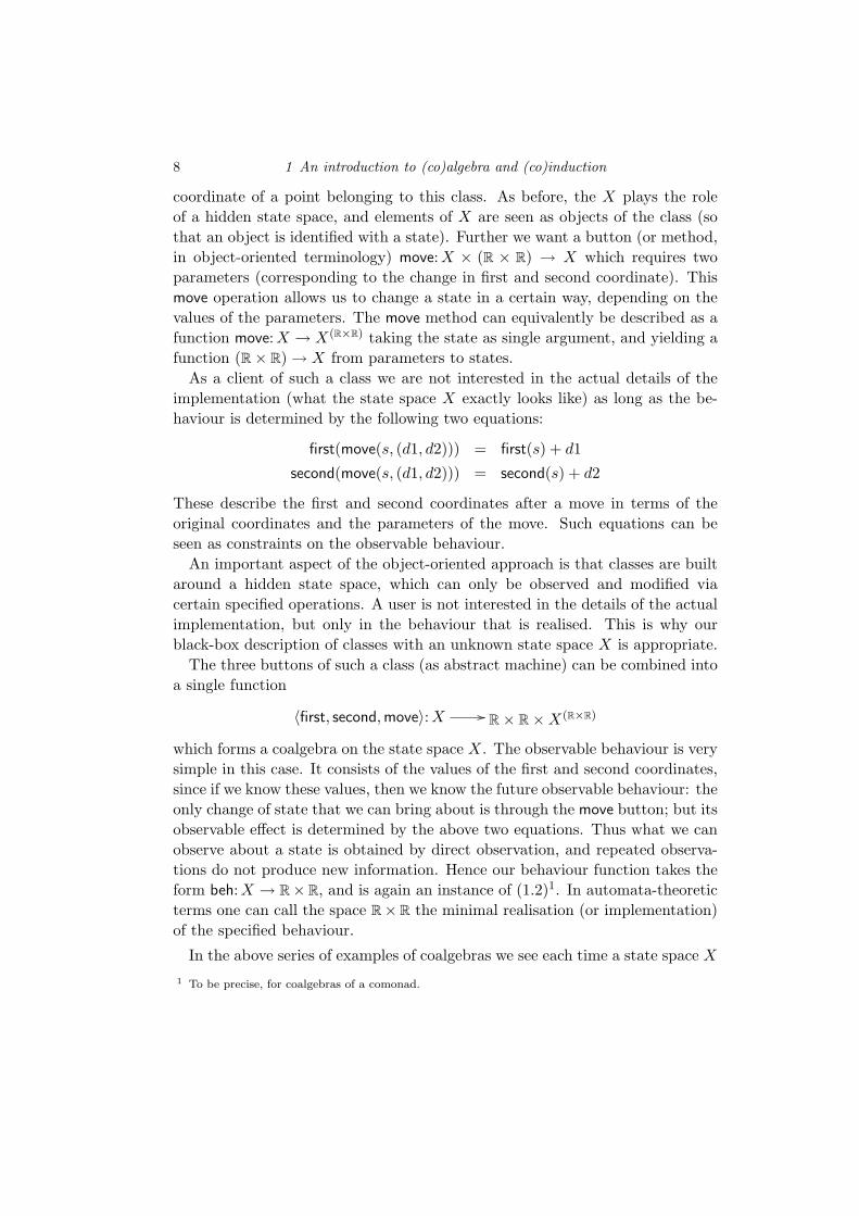
coordinate of a point belonging to this class. As before, the X plays the roleof a hidden state space, and elements of X are seen as objects of the class (sothat an object is identified with a state). Further we want a button (or method,in object-oriented terminology) move:X × (R × R) → X which requires twoparameters (corresponding to the change in first and second coordinate). Thismove operation allows us to change a state in a certain way, depending on thevalues of the parameters. The move method can equivalently be described as afunction move:X → X(R×R) taking the state as single argument, and yielding afunction (R× R)→ X from parameters to states.

As a client of such a class we are not interested in the actual details of theimplementation (what the state space X exactly looks like) as long as the be-haviour is determined by the following two equations:

first(move(s, (d1, d2))) = first(s) + d1

second(move(s, (d1, d2))) = second(s) + d2

These describe the first and second coordinates after a move in terms of theoriginal coordinates and the parameters of the move. Such equations can beseen as constraints on the observable behaviour.

An important aspect of the object-oriented approach is that classes are builtaround a hidden state space, which can only be observed and modified viacertain specified operations. A user is not interested in the details of the actualimplementation, but only in the behaviour that is realised. This is why ourblack-box description of classes with an unknown state space X is appropriate.

The three buttons of such a class (as abstract machine) can be combined intoa single function

〈first, second,move〉:X // R× R×X(R×R)

which forms a coalgebra on the state space X. The observable behaviour is verysimple in this case. It consists of the values of the first and second coordinates,since if we know these values, then we know the future observable behaviour: theonly change of state that we can bring about is through the move button; but itsobservable effect is determined by the above two equations. Thus what we canobserve about a state is obtained by direct observation, and repeated observa-tions do not produce new information. Hence our behaviour function takes theform beh:X → R×R, and is again an instance of (1.2)1. In automata-theoreticterms one can call the space R×R the minimal realisation (or implementation)of the specified behaviour.

In the above series of examples of coalgebras we see each time a state space X1 To be precise, for coalgebras of a comonad.


about which we make no assumptions. On this state space a function is definedof the form

f : X → X

where the box on the right is some expression involving X again. Later this willbe identified as a functor. The function f often consists of different components,which allow us either to observe some aspect of the state space directly, or tomove on to next states. We have limited access to this state space in the sensethat we can only observe or modify it via these specified operations. In sucha situation all that we can describe about a particular state is its behaviour,which arises by making successive observations. This will lead to the notion ofbisimilarity of states: it expresses of two states that we cannot distinguish themvia the operations that are at our disposal, i.e. that they are “equal as far as wecan see”. But this does not mean that these states are also identical as elementsof X. Bisimilarity is an important, and typically coalgebraic, concept.

The above examples are meant to suggest the difference between construc-tion in algebra, and observation in coalgebra. This difference will be describedmore formally below. In practice it is not always completely straightforwardto distinguish between algebraic and coalgebraic aspects, for the following tworeasons.

(1) Certain abstract operations, like X × A→ X, can be seen as both alge-braic and coalgebraic. Algebraically, such an operation allows us to buildnew elements in X starting from given elements in X and parameters inA. Coalgebraically, this operation is often presented in the equivalentfrom X → XA using function types. It is then seen as acting on thestate space X, and yielding for each state a function from A to X whichproduces for each parameter element in A a next state. The contextshould make clear which view is prevalent. But operations of the formA→ X are definitely algebraic (because they gives us information abouthow to put elements in X), and operations of the form X → A arecoalgebraic (because they give us observable attribute values holding forelements of X). A further complication at this point is that on an initialalgebra X one may have operations of the form X → A, obtained byinitiality. An example is the length function on lists. Such operations arederived, and are not an integral part of the (definition of the) algebra.Dually, one may have derived operations A→ X on a final coalgebra X.

(2) Algebraic and coalgebraic structures may be found in different hierarchiclayers. For example, one can start with certain algebras describing one’sapplication domain. On top of these one can have certain dynamical sys-


tems (processes) as coalgebras, involving such algebras (e.g. as codomainsof attributes). And such coalgebraic systems may exist in an algebra ofprocesses.

A concrete example of such layering of coalgebra on top of algebra is givenby Plotkin’s so-called structural operational semantics [Plo81]. It involves atransition system (a coalgebra) describing the operational semantics of somelanguage, by giving the transition rules by induction on the structure of theterms of the language. The latter means that the set of terms of the languageis used as (initial) algebra. See Section 1.8 and [RT94, Tur96] for a furtherinvestigation of this perspective. Hidden sorted algebras, see [GM94, GD94,BD94, GM96, Mal96] can be seen as other examples: they involve “algebras”with “invisible” sorts, playing a (coalgebraic) role of a state space. Coinductionis used to reason about such hidden state spaces, see [GM96].

1.3 Inductive and coinductive definitions

In the previous section we have seen that “constructor” and “destructor/observer”operations play an important role for algebras and coalgebras, respectively. Con-structors tell us how to generate our (algebraic) data elements: the empty listconstructor nil and the prefix operation cons generate all finite lists. And de-structors (or observers, or transition functions) tell us what we can observeabout our data elements: the head and tail operations tell us all about infinitelists: head gives a direct observation, and tail returns a next state.

Once we are aware of this duality between constructing and observing, it iseasy to see the difference between inductive and coinductive definitions (relativeto given collections of constructors and destructors):

In an inductive definition of a function f ,one defines the value of f on all constructors.

And:

In a coinductive definition of a function f ,one defines the values of all destructors on each outcome f(x).

Such a coinductive definition determines the observable behaviour of each f(x).We shall illustrate inductive and coinductive definitions in some examples

involving finite lists (with constructors nil and cons) and infinite lists (withdestructors head and tail) over a fixed dataset A, as in the previous section.We assume that inductive definitions are well-known, so we only mention twotrivial examples: the (earlier mentioned) function len from finite lists to natural

1.3 Inductive and coinductive definitions 11

numbers giving the length, and the function empty? from finite lists to booleans{true, false} telling whether a list is empty or not:{

len(nil) = 0len(cons(a, σ)) = 1 + len(σ).

{empty?(nil) = true

empty?(cons(a, σ)) = false.

Typically in such inductive definitions, the constructors on the left hand sideappear “inside” the function that we are defining. The example of empty? above,where this does not happen, is a degenerate case.

We turn to examples of coinductive definitions (on infinite lists, say of type A).If we have a function f :A→ A, then we would like to define an extension ext(f)of f mapping an infinite list to an infinite list by applying f componentwise.According to the above coinductive definition scheme we have to give the valuesof the destructors head and tail for a sequence ext(f)(σ). They should be:{

head(ext(f)(σ)) = f(head(σ))tail(ext(f)(σ)) = ext(f)(tail(σ))

Here we clearly see that on the left hand side, the function that we are definingoccurs “inside” the destructors. At this stage it is not yet clear if ext(f) iswell-defined, but this is not our concern at the moment.

Alternatively, using the transition relation notation from Example (iv) in theprevious section, we can write the definition of ext(f) as:

σa−→ σ′

ext(f)(σ)f(a)−→ ext(f)(σ′)

Suppose next, that we wish to define an operation even which takes an infinitelist, and produces a new infinite list which contains (in order) all the elementsoccurring in evenly numbered places of the original list. That is, we would likethe operation even to satisfy

even(σ(0), σ(1), σ(2), . . .) = (σ(0), σ(2), σ(4), . . .) (1.3)

A little thought leads to the following definition clauses.{head(even(σ)) = head(σ)tail(even(σ)) = even(tail(tail(σ)))

(1.4)

Or, in the transition relation notation:

σa−→ σ′

a′−→ σ′′

even(σ) a−→ even(σ′′)

Let us convince ourselves that this definition gives us what we want. The firstclause in (1.4) says that the first element of the list even(σ) is the first element


of σ. The next element in even(σ) is head(tail(even(σ))), and can be computedas

head(tail(even(σ))) = head(even(tail(tail(σ)))) = head(tail(tail(σ))).

Hence the second element in even(σ) is the third element in σ. It is not hard toshow for n ∈ N that head(tail(n)(even(σ))) is the same as head(tail(2n)(σ)).

In a similar way one can coinductively define a function odd which keeps allthe oddly listed elements. But it is much easier to define odd as: odd = even◦tail.

As another example, we consider the merge of two infinite lists σ, τ into asingle list, by taking elements from σ and τ in turn, starting with σ, say. Acoinductive definition of such a function merge requires the outcomes of thedestructors head and tail on merge(σ, τ). They are given as:{

head(merge(σ, τ)) = head(σ)tail(merge(σ, τ)) = merge(τ, tail(σ))

In transition system notation, this definition looks as follows.

σa−→ σ′

merge(σ, τ) a−→ merge(τ, σ′)

Now one can show that the n-th element of σ occurs as 2n-th element inmerge(σ, τ), and that the n-th element of τ occurs as (2n + 1)-th element ofmerge(σ, τ):

head(tail(2n)(merge(σ, τ))) = head(tail(n)(σ))

head(tail(2n+1)(merge(σ, τ))) = head(tail(n)(τ)).

One can also define a function merge2,1(σ, τ) which takes two elements of σ forevery element of τ (see Exercise 1.10.6).

An obvious result that we would like to prove is: merging the lists of evenlyand oddly occuring elements in a list σ returns the original list σ. That is:merge(even(σ), odd(σ)) = σ. From what we have seen above we can easilycompute that the n-th elements on both sides are equal:

head(tail(n)(merge(even(σ), odd(σ))))

=

{head(tail(m)(even(σ))) if n = 2mhead(tail(m)(odd(σ))) if n = 2m+ 1

=

{head(tail(2m)(σ)) if n = 2mhead(tail(2m+1)(σ)) if n = 2m+ 1

= head(tail(n)(σ)).

There is however a more elegant coinductive proof-technique, which will be

1.4 Functoriality of products, coproducts and powersets 13

presented later: in Example 1.6.3 using uniqueness—based on the finality dia-gram (1.2)—and in the beginning of Section 1.7 using bisimulations.

1.4 Functoriality of products, coproducts and powersets

In the remainder of this paper we shall put the things we have discussed sofar in a general framework. Doing so properly requires a certain amount ofcategory theory. We do not intend to describe the relevant matters at thehighest level of abstraction, making full use of category theory. Instead, weshall work mainly with ordinary sets. That is, we shall work in the universegiven by the category of sets and functions. What we do need is that manyoperations on sets are “functorial”. This means that they do not act only onsets, but also on functions between sets, in an appropriate manner. This isfamiliar in the computer science literature, not in categorical terminology, butusing a “map” terminology. For example, if list(A) = A? describes the set offinite lists of elements of a set A, then for a function f :A → B one can definea function list(A) → list(B) between the corresponding sets of lists, which isusually called1 map list(f). It sends a finite list (a1, . . . , an) of elements of Ato the list (f(a1), . . . , f(an)) of elements of B, by applying f elementwise. Itis not hard to show that this map list operation preserves identity functionsand composite functions, i.e. that map list(idA) = idlist(A) and map list(g ◦ f) =map list(g) ◦ map list(f). This preservation of identities and compositions isthe appropriateness that we mentioned above. In this section we concentrateon such functoriality of several basic operations, such as products, coproducts(disjoint unions) and powersets. It will be used in later sections.

We recall that for two sets X,Y the Cartesian product X × Y is the set ofpairs

X × Y = {(x, y) | x ∈ X and y ∈ Y }.

There are then obvious projection functions π:X × Y → X and π′:X × Y → Y

by π(x, y) = x and π′(x, y) = y. Also, for functions f :Z → X and g:Z → Y

there is a unique “pair function” 〈f, g〉:Z → X × Y with π ◦ 〈f, g〉 = f andπ′ ◦ 〈f, g〉 = g, namely 〈f, g〉(z) = (f(z), g(z)) ∈ X × Y for z ∈ Z. Notice that〈π, π′〉 = id:X × Y → X × Y and that 〈f, g〉 ◦ h = 〈f ◦ h, g ◦ h〉:W → X × Y ,for functions h:W → Z.

Interestingly, the product operation (X,Y ) 7→ X × Y does not only applyto sets, but also to functions: for functions f :X → X ′ and g:Y → Y ′ we candefine a function X × X ′ → Y × Y ′ by (x, y) 7→ (f(x), g(y)). One writes this

1 In the category theory literature one uses the same name for the actions of a functor on objects andon morphisms; this leads to the notation list(f) or f? for this function map list(f).


function as f × g:X × Y → X ′ × Y ′, whereby the symbol × is overloaded: itis used both on sets and on functions. We note that f × g can be described interms of projections and pairing as f × g = 〈f ◦ π, g ◦ π′〉. It is easily verifiedthat the operation × on functions satisfies

idX × idY = idX×Y and (f ◦ h)× (g ◦ k) = (f × g) ◦ (h× k).

This expresses that the product × is functorial : it does not only apply to sets,but also to functions; and it does so in such a way that identity maps andcomposites are preserved.

Many more operations are functorial. Also the coproduct (or disjoint union,or sum) + is. For sets X,Y we write their disjoint union as X + Y . Explicitly:

X + Y = {〈0, x〉 | x ∈ X} ∪ {〈1, y〉 | y ∈ Y }.

The first components 0 and 1 serve to force this union to be disjoint. These“tags” enables us to recognise the elements of X and of Y inside X+Y . Insteadof projections as above we now have “coprojections” κ:X → X+Y and κ′:Y →X + Y going in the other direction. One puts κ(x) = 〈0, x〉 and κ′(y) = 〈1, y〉.And instead of tupleing we now have “cotupleing” (sometimes called “sourcetupleing”): for functions f :X → Z and g:Y → Z there is a unique function[f, g]:X + Y → Z with [f, g] ◦ κ = f and [f, g] ◦ κ′ = g. One defines [f, g] bycase distinction:

[f, g](w) ={f(x) if w = 〈0, x〉g(y) if w = 〈1, y〉.

Notice that [κ, κ′] = id and h ◦ [f, g] = [h ◦ f, h ◦ g].This is the coproduct X + Y on sets. We can extend it to functions in the

following way. For f :X → X ′ and g:Y → Y ′ there is a function f +g:X+Y →X ′ + Y ′ by

(f + g)(w) ={〈0, f(x)〉 if w = 〈0, x〉〈1, g(y)〉 if w = 〈1, y〉.

Equivalently, we could have defined: f + g = [κ ◦ f, κ′ ◦ g]. This operation + onfunctions preserves identities and composition:

idX + idY = idX+Y and (f ◦ h) + (g ◦ k) = (f + g) ◦ (h+ k).

We should emphasise that this coproduct + is very different from ordinaryunion ∪. For example, ∪ is idempotent: X ∪X = X, but there is not odd anisomorphism between X +X and X (if X 6= ∅).

For a fixed set A, the assignment X 7→ XA = {f | f is a function A→ X} isfunctorial: a function g:X → Y yields a function gA:XA → Y A sending f ∈ XA

to (g ◦ f) ∈ Y A. Clearly, idA = id and (h ◦ g)A = hA ◦ gA.

1.4 Functoriality of products, coproducts and powersets 15

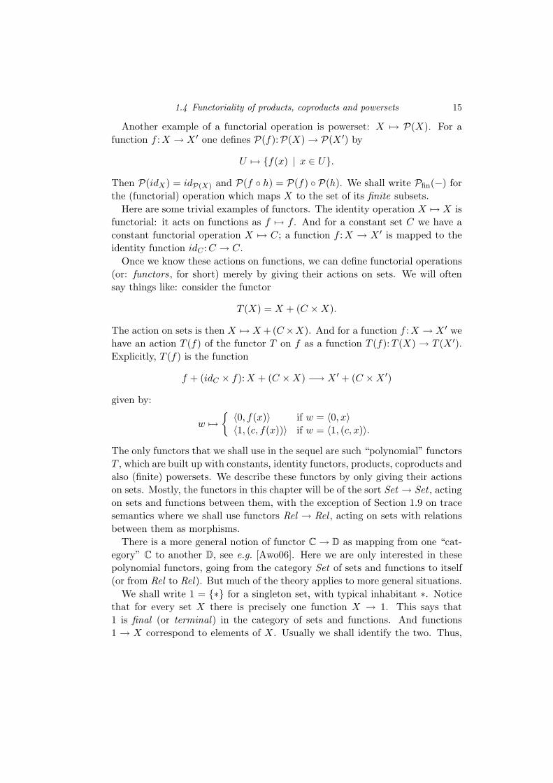
Another example of a functorial operation is powerset: X 7→ P(X). For afunction f :X → X ′ one defines P(f):P(X)→ P(X ′) by

U 7→ {f(x) | x ∈ U}.

Then P(idX) = idP(X) and P(f ◦ h) = P(f) ◦ P(h). We shall write Pfin(−) forthe (functorial) operation which maps X to the set of its finite subsets.

Here are some trivial examples of functors. The identity operation X 7→ X isfunctorial: it acts on functions as f 7→ f . And for a constant set C we have aconstant functorial operation X 7→ C; a function f :X → X ′ is mapped to theidentity function idC :C → C.

Once we know these actions on functions, we can define functorial operations(or: functors, for short) merely by giving their actions on sets. We will oftensay things like: consider the functor

T (X) = X + (C ×X).

The action on sets is then X 7→ X+ (C×X). And for a function f :X → X ′ wehave an action T (f) of the functor T on f as a function T (f):T (X) → T (X ′).Explicitly, T (f) is the function

f + (idC × f):X + (C ×X) −→ X ′ + (C ×X ′)

given by:

w 7→{〈0, f(x)〉 if w = 〈0, x〉〈1, (c, f(x))〉 if w = 〈1, (c, x)〉.

The only functors that we shall use in the sequel are such “polynomial” functorsT , which are built up with constants, identity functors, products, coproducts andalso (finite) powersets. We describe these functors by only giving their actionson sets. Mostly, the functors in this chapter will be of the sort Set → Set , actingon sets and functions between them, with the exception of Section 1.9 on tracesemantics where we shall use functors Rel → Rel , acting on sets with relationsbetween them as morphisms.

There is a more general notion of functor C→ D as mapping from one “cat-egory” C to another D, see e.g. [Awo06]. Here we are only interested in thesepolynomial functors, going from the category Set of sets and functions to itself(or from Rel to Rel). But much of the theory applies to more general situations.

We shall write 1 = {∗} for a singleton set, with typical inhabitant ∗. Noticethat for every set X there is precisely one function X → 1. This says that1 is final (or terminal) in the category of sets and functions. And functions1 → X correspond to elements of X. Usually we shall identify the two. Thus,


for example, we sometimes write the empty list as nil : 1→ A? so that it can becotupled with the function cons : A×A? → A? into the algebra

[nil, cons]: 1 + (A×A?)→ A?

that will be studied more deeply in Example 1.5.6.We write 0 for the empty set. For every set X there is precisely one function

0 → X, namely the empty function. This property is the initiality of 0. Thesesets 1 and 0 can be seen as the empty product and coproduct.

We list some useful isomorphisms.

X × Y ∼= Y ×X X + Y ∼= Y +X

1×X ∼= X 0 +X ∼= X

X × (Y × Z) ∼= (X × Y )× Z X + (Y + Z) ∼= (X + Y ) + Z

X × 0 ∼= 0 X × (Y + Z) ∼= (X × Y ) + (X × Z).

The last two isomorphisms describe the distribution of products over finite co-products. We shall often work “up-to” the above isomorphisms, so that wecan simply write an n-ary product as X1 × · · · × Xn without bothering aboutbracketing.

1.5 Algebras and induction

In this section we start by showing how polynomial functors—as introduced inthe previous section—can be used to describe signatures of operations. Algebrasof such functors correspond to models of such signatures. They consist of acarrier set with certain functions interpreting the operations. A general notionof homomorphism is defined between such algebras of a functor. This allowsus to define initial algebras by the following property: for an arbitrary algebrathere is precisely one homomorphism from the initial algebra to this algebra.This turns out to be a powerful notion. It captures algebraic structures whichare generated by constructor operations, as will be shown in several examples.Also, it gives rise to the familiar principles of definition by induction and proofby induction.

We start with an example. Let T be the polynomial functor T (X) = 1 +X + (X × X), and consider for a set U a function a:T (U) → U . Such a mapa may be identified with a 3-cotuple [a1, a2, a3] of maps a1: 1 → U , a2:U →U and a3:U × U → U giving us three separate functions going into the setU . They form an example of an algebra (of the functor T ): a set togetherwith a (cotupled) number of functions going into that set. For example, if onehas a group G, with unit element e: 1 → G, inverse function i:G → G and

1.5 Algebras and induction 17

multiplication function m:G×G→ G, then one can organise these three mapsas an algebra [e, i,m]:T (G) → G via cotupling1. The shape of the functor Tdetermines a certain signature of operations. Had we taken a different functorS(X) = 1 + (X ×X), then maps (algebras of S) S(U)→ U would capture pairsof functions 1→ U , U × U → U (e.g. of a monoid).

Definition 1.5.1 Let T be a functor. An algebra of T (or, a T -algebra) is apair consisting of a set U and a function a:T (U)→ U .

We shall call the set U the carrier of the algebra, and the function a thealgebra structure, or also the operation of the algebra.

For example, the zero and successor functions 0: 1 → N, S: N → N on thenatural numbers form an algebra [0, S]: 1+N→ N of the functor T (X) = 1+X.And the set of A-labeled finite binary trees Tree(A) comes with functions nil: 1→Tree(A) for the empty tree, and node: Tree(A) × A × Tree(A) → Tree(A) forconstructing a tree out of two (sub)trees and a (node) label. Together, nil andnode form an algebra 1 + (Tree(A) × A × Tree(A)) → Tree(A) of the functorS(X) = 1 + (X ×A×X).

We illustrate the link between signatures (of operations) and functors withfurther details. Let Σ be a (single-sorted, or single-typed) signature, given bya finite collection Σ of operations σ, each with an arity ar(σ) ∈ N. Each σ ∈ Σwill be understood as an operation

σ:X × · · · ×X︸︷︷︸ar(σ) times

−→ X

taking ar(σ) inputs of some type X, and producing an output of type X. Withthis signature Σ, say with set of operations {σ1, . . . , σn} we associate a functor

TΣ(X) = Xar(σ1) + · · ·+Xar(σn),

where for m ∈ N the set Xm is the m-fold product X × · · · × X. An al-gebra a:TΣ(U) → U of this functor TΣ can be identified with an n-cotuplea = [a1, . . . an]:Uar(σ1) + · · · + Uar(σn) → U of functions ai:Uar(σi) → U inter-preting the operations σi in Σ as functions on U . Hence algebras of the functorTΣ correspond to models of the signature Σ. One sees how the arities in thesignature Σ determine the shape of the associated functor TΣ. Notice that asspecial case when an arity of an operation is zero we have a constant in Σ. Ina TΣ-algebra TΣ(U) → U we get an associated map U0 = 1 → U giving us anelement of the carrier set U as interpretation of the constant. The assumptionthat the signature Σ is finite is not essential for the correspondence between1 Only the group’s operations, and not its equations, are captured in this map T (G)→ G.


models of Σ and algebras of TΣ; if Σ is infinite, one can define TΣ via an infinitecoproduct, commonly written as TΣ(X) =

∐σ∈ΣX

ar(σ).Polynomial functors T built up from the identity functor, products and co-

products (without constants) have algebras which are models of the kind of sig-natures Σ described above. This is because by the distribution of products overcoproducts one can always write such a functor in “disjunctive normal form” asT (X) = Xm1 + · · ·+Xmn for certain natural numbers n and m1, . . . ,mn. Theessential role of the coproducts is to combine multiple operations into a singleoperation.

The polynomial functors that we use are not only of this form T (X) = Xm1 +· · ·+Xmn , but may also involve constant sets. This is quite useful, for example,to describe for an arbitrary set A a signature for lists of A’s, with functionsymbols nil: 1 → X for the empty list, and cons:A × X → X for prefixing anelement of type A to a list. A model (interpretation) for such a signature isan algebra T (U) → U of the functor T (X) = 1 + (A×X) associated with thissignature.

We turn to “homomorphisms of algebras”, to be understood as structurepreserving functions between algebras (of the same signature, or functor). Sucha homomorphism is a function between the carrier sets of the algebras whichcommutes with the operations. For example, suppose we have two algebras`1: 1 → U1, c1:A × U1 → U1 and `2: 1 → U2, c2:A × U2 → U2 of the above listsignature. A homomorphism of algebras from the first to the second consists of afunction f :U1 → U2 between the carriers with f ◦`1 = `2 and f ◦c1 = c2◦(id×f).In two diagrams:

1

`1��

1

`2��

U1f

// U2

and

A× U1id× f //

c1��

A× U2

c2��

U1f

// U2

Thus, writing n1 = `1(∗) and n2 = `2(∗), these diagrams express that f(n1) = n2

and f(c1(a, x)) = c2(a, f(x)), for a ∈ A and x ∈ U1.These two diagrams can be combined into a single diagram:

1 + (A× U1)id+ (id× f)

//

[`1, c1]��

1 + (A× U2)

[`2, c2]��

U1f

// U2


i.e., for the list-functor T (X) = 1 + (A×X),

T (U1)T (f)

//

[`1, c1]��

T (U2)

[`2, c2]��

U1f

// U2

The latter formulation is entirely in terms of the functor involved. This moti-vates the following definition.

Definition 1.5.2 Let T be a functor with algebras a:T (U)→ U and b:T (V )→V . A homomorphism of algebras (also called a map of algebras, or an algebramap) from (U, a) to (V, b) is a function f :U → V between the carrier sets whichcommutes with the operations: f ◦ a = b ◦ T (f) in

T (U)T (f)

//

a��

T (V )

b��

Uf

// V

As a triviality we notice that for an algebra a:T (U)→ U the identity functionU → U is an algebra map (U, a) → (U, a). And we can compose algebra mapsas functions: given two algebra maps(

T (U) a−→ U) f //

(T (V ) b−→ V

)g //(T (W ) c−→W

)then the composite function g ◦ f :U → W is an algebra map from (U, a) to(W, c). This is because g ◦ f ◦ a = g ◦ b ◦ T (f) = c ◦ T (g) ◦ T (f) = c ◦ T (g ◦ f),see the following diagram.

T (U)

a��

T (f)//

T (g ◦ f)++

T (V )

b��

T (g)// T (W )

c��

Uf //

g ◦ f

44Vg // W

Thus: algebras and their homomorphisms form a category.Now that we have a notion of homomorphism of algebras we can formulate

the important concept of “initiality” for algebras.


Definition 1.5.3 An algebra a:T (U) → U of a functor T is initial if for eachalgebra b:T (V ) → V there is a unique homomorphism of algebras from (U, a)to (V, b). Diagrammatically we express this uniqueness by a dashed arrow, callit f , in

T (U)

a��

//______T (f)

T (V )

b��

U //________f

V

We shall sometimes call this f the “unique mediating algebra map”.

We emphasise that unique existence has two aspects, namely existence of analgebra map out of the initial algebra to another algebra, and uniqueness, in theform of equality of any two algebra maps going out of the initial algebra to someother algebra. Existence will be used as an (inductive) definition principle, anduniqueness as an (inductive) proof principle.

As a first example, we shall describe the set N of natural numbers as initialalgebra.

Example 1.5.4 Consider the set N of natural number with its zero and suc-cessor function 0: 1→ N and S: N→ N. These functions can be combined into asingle function [0, S]: 1+N→ N, forming an algebra of the functor T (X) = 1+X.We will show that this map [0, S]: 1+N→ N is the initial algebra of this functorT . And this characterises the set of natural numbers (up-to-isomorphism), byLemma 1.5.5 (ii) below.

To prove initiality, assume we have an arbitrary set U carrying a T -algebrastructure [u, h]: 1 + U → U . We have to define a “mediating” homomorphismf : N→ U . We try iteration:

f(n) = h(n)(u)

where we simply write u instead of u(∗). That is,

f(0) = u and f(n+ 1) = h(f(n)).

These two equations express that we have a commuting diagram

1 + N

[0, S]��

id+ f // 1 + U

[u, h]��

Nf

// U


making f a homomorphism of algebras. This can be verified easily by distin-guishing for an arbitrary element x ∈ 1 + N in the upper-left corner the twocases x = (0, ∗) = κ(∗) and x = (1, n) = κ′(n), for n ∈ N. In the first casex = κ(∗) we get

f([0, S](κ(∗))) = f(0) = u = [u, h](κ(∗)) = [u, h]((id+ f)(κ(∗))).

In the second case x = κ′(n) we similarly check:

f([0, S](κ′(n))) = f(S(n)) = h(f(n)) = [u, h](κ′(f(n))) = [u, h]((id+f)(κ′(n))).

Hence we may conclude that f([0, S](x)) = [u, h]((id+ f)(x)), for all x ∈ 1 + N,i.e. that f ◦ [0, S] = [u, h] ◦ (id+ f).

This looks promising, but we still have to show that f is the only map makingthe diagram commute. If g: N→ U also satisfies g ◦ [0, S] = [u, h]◦ (id+ g), theng(0) = u and g(n+ 1) = h(g(n)), by the same line of reasoning followed above.Hence g(n) = f(n) by induction on n, so that g = f : N→ U .

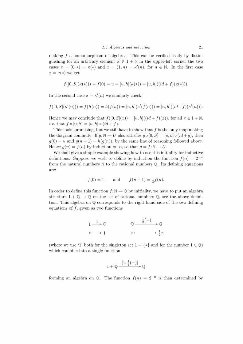
We shall give a simple example showing how to use this initiality for inductivedefinitions. Suppose we wish to define by induction the function f(n) = 2−n

from the natural numbers N to the rational numbers Q. Its defining equationsare:

f(0) = 1 and f(n+ 1) = 12f(n).

In order to define this function f : N→ Q by initiality, we have to put an algebrastructure 1 + Q → Q on the set of rational numbers Q, see the above defini-tion. This algebra on Q corresponds to the right hand side of the two definingequations of f , given as two functions

1 1 // Q Q12(−)

// Q

∗ � // 1 x � // 12x

(where we use ‘1’ both for the singleton set 1 = {∗} and for the number 1 ∈ Q)which combine into a single function

1 + Q[1, 1

2(−)]// Q

forming an algebra on Q. The function f(n) = 2−n is then determined by


initiality as the unique function making the following diagram commute.

1 + N

[0, S]��

id+ f // 1 + Q

[1, 12(−)]

��N

f// Q

This shows how initiality can be used to define functions by induction. It requiresthat one puts an appropriate algebra structure on the codomain (i.e. the range)of the intended function, corresponding to the induction clauses that determinethe function.

We emphasise that the functor T is a parameter in Definitions 1.5.2 and 1.5.3of “homomorphism” and “initiality” for algebras, yielding uniform notions forall functors T (representing certain signatures). It turns out that initial algebrashave certain properties, which can be shown for all functors T at once. Dia-grams are convenient in expressing and proving these properties, because theydisplay information in a succinct way. And they are useful both in existenceand uniqueness arguments.

Lemma 1.5.5 Let T be a functor.(i) Initial T -algebras, if they exist, are unique, up-to-isomorphism of algebras.

That is, if we have two initial algebras a:T (U) → U and a′:T (U ′) → U ′ of T ,then there is a unique isomorphism f :U

∼=→ U ′ of algebras:

T (U)

a��

∼=T (f)

// T (U ′)

a′��

U ∼=f // U ′

(ii) The operation of an initial algebras is an isomorphism: if a:T (U)→ U isinitial algebra, then a has an inverse a−1:U → T (U).

The first point tells us that a functor can have (essentially) at most one initialalgebra1. Therefore, we often speak of the initial algebra of a functor T . And thesecond point—which is due to Lambek—says that an initial algebra T (U)→ U

is a fixed point T (U) ∼= U of the functor T . Initial algebras may be seen asgeneralizations of least fixed points of monotone functions, since they have a(unique) map into an arbitrary algebra, see Exercise 1.10.3.

1 This is a more general property of initial objects in a category.


Proof (i) Suppose both a:T (U) → U and a′:T (U ′) → U ′ are initial algebrasof the functor T . By initiality of a there is a unique algebra map f :U → U ′.Similarly, by initiality of a′ there is a unique algebra map f ′:U ′ → U in theother direction:

T (U) //______T (f)

a��

T (U ′)

a′��

U //________f

U ′

T (U ′)

a′��

//______T (f ′)

T (U)

a��

U ′ //________f ′

U

Here we use the existence parts of initiality. The uniqueness part gives us thatthe two resulting algebra maps (U, a)→ (U, a), namely f ◦ f ′ and id in:

T (U)

a��

T (f)// T (U ′)

a′��

T (f ′)// T (U)

a��

Uf

// U ′f ′

// U

and

T (U)

a��

T (id)// T (U)

a��

Uid

// U

must be equal, i.e. that f ′ ◦ f = id. Uniqueness of algebra maps (U ′, a′) →(U ′, a′) similarly yields f ◦ f ′ = id. Hence f is an isomorphism of algebras.

(ii) Let a:T (U)→ U be initial T -algebra. In order to show that the function ais an isomorphism, we have to produce an inverse function U → T (U). Initialityof (U, a) can be used to define functions out of U to arbitrary algebras. Since weseek a function U → T (U), we have to put an algebra structure on the set T (U).A moment’s thought yields a candidate, namely the result T (a):T (T (U)) →T (U) of applying the functor T to the function a. This function T (a) gives byinitiality of a:T (U)→ U rise to a function a′:U → T (U) with T (a)◦T (a′) = a′◦ain:

T (U)

a��

//______T (a′)

T (T (U))

T (a)��

U //________a′

T (U)


The function a ◦ a′:U → U is an algebra map (U, a)→ (U, a):

T (U)

a��

T (a′)// T (T (U))

T (a)//

T (a)��

T (U)

a��

Ua′

// T (U) a// U

so that a ◦ a′ = id by uniqueness of algebra maps (U, a)→ (U, a). But then

a′ ◦ a = T (a) ◦ T (a′) by definition of a′

= T (a ◦ a′) since T preserves composition

= T (id) as we have just seen

= id since T preserves identities.

Hence a:T (U)→ U is an isomorphism with a′ as its inverse. �

From now on we shall often write an initial T -algebra as a map a:T (U)∼=→ U ,

making this isomorphism explicit.

Example 1.5.6 Let A be fixed set and consider the functor T (X) = 1+(A×X)that we used earlier to capture models of the list signature 1→ X, A×X → X.We claim that the initial algebra of this functor T is the set A? = list(A) =⋃n∈N A

n of finite sequences of elements of A, together with the function (orelement) 1→ A? given by the empty list nil = (), and the function A×A? → A?

which maps an element a ∈ A and a list α = (a1, . . . , an) ∈ A? to the listcons(a, α) = (a, a1, . . . , an) ∈ A?, obtained by prefixing a to α. These twofunctions can be combined into a single function [nil, cons]: 1 + (A× A?)→ A?,which, as one easily checks, is an isomorphism. But this does not yet mean thatit is the initial algebra. We will check this explicitly.

For an arbitrary algebra [u, h]: 1 + (A×U)→ U of the list-functor T we havea unique homomorphism f :A? → U of algebras:

1 + (A×A?)

[nil, cons]��

id+ (id× f)// 1 + (A× U)

[u, h]��

A?f

// U

namely

f(α) ={u if α = nil

h(a, f(β)) if α = cons(a, β).


We leave it to the reader to verify that f is indeed the unique function A? → U

making the diagram commute.Again we can use this initiality of A? to define functions by induction (for

lists). As example we take the length function len:A? → N, described already inthe beginning of Section 1.2. In order to define it by initiality, it has to arise froma list-algebra structure 1 +A× N→ N on the natural numbers N. This algebrastructure is the cotuple of the two functions 0: 1 → N and S ◦ π′:A × N → N.Hence len is determined as the unique function in the following initiality diagram.

1 + (A×A?)

[nil, cons] ∼=��

id+ (id× len)// 1 + (A× N)

[0, S ◦ π′]��

A?len

// N

The algebra structure that we use on N corresponds to the defining clauseslen(nil) = 0 and len(cons(a, α)) = S(len(α)) = S(len(π′(a, α))) = S(π′(id ×len)(a, α)).

We proceed with an example showing how proof by induction involves usingthe uniqueness of a map out of an initial algebra. Consider therefore the “dou-bling” function d:A? → A? which replaces each element a in a list α by twoconsecutive occurrences a, a in d(α). This function is defined as the unique onemaking the following diagram commute.

1 + (A×A?)


id+ (id× d)// 1 + (A×A?)

[nil, λ(a, α). cons(a, cons(a, α))]��

A?d

// A?

That is, d is defined by the induction clauses d(nil) = nil and d(cons(a, α)) =cons(a, cons(a, d(α)). We wish to show that the length of the list d(α) is twicethe length of α, i.e. that

len(d(α)) = 2 · len(α).

The ordinary induction proof consists of two steps:

len(d(nil)) = len(nil) = 0 = 2 · 0 = 2 · len(nil)


Andlen(d(cons(a, α))) = len(cons(a, cons(a, d(α))))

= 1 + 1 + len(d(α))(IH)= 2 + 2 · len(α)

= 2 · (1 + len(α))

= 2 · len(cons(a, α)).

The “initiality” induction proof of the fact len ◦ d = 2 · (−) ◦ len uses uniquenessin the following manner. Both len◦d and 2·(−)◦len are homomorphism from the(initial) algebra (A?, [nil, cons]) to the algebra (N, [0, S ◦S ◦π′]), so they must beequal by initiality. First we check that len ◦ d is an appropriate homomorphismby inspection of the following diagram.

1 + (A×A?)

[nil, cons]∼=��

id+ (id× d)// 1 + (A×A?)

[nil, λ(a, α). cons(a, cons(a, α))]��

id+ (id× len)// 1 + (A× N)

[0, S ◦ S ◦ π′]��

A?d

// A?len

// N

The rectangle on the left commutes by definition of d. And commutation of therectangle on the right follows easily from the definition of len. Next we checkthat 2 · (−) ◦ len is also a homomorphism of algebras:

1 + (A×A?)

[nil, cons]∼=

��

id+ (id× len)// 1 + (A× N)

id+ π′��

id+ (id× 2 · (−))// 1 + (A× N)

id+ π′��

ED

BC[0, S◦S◦π′]

oo

1 + N

[0, S] ∼=��

id+ 2 · (−)// 1 + N

[0, S◦S]��

A?len

// N2 · (−)

// N

The square on the left commutes by definition of len. Commutation of the uppersquare on the right follows from an easy computation. And the lower square onthe right may be seen as defining the function 2 · (−): N → N by the clauses:2 · 0 = 0 and 2 · (S(n)) = S(S(2 · n))—which we took for granted in the earlier“ordinary” proof.

We conclude our brief discussion of algebras and induction with a few remarks.

(1) Given a number of constructors one can form the carrier set of the asso-ciated initial algebra as the set of ‘closed’ terms (or ‘ground’ terms, not


containing variables) that can be formed with these constructors. Forexample, the zero and successor constructors 0: 1 → X and S:X → X

give rise to the set of closed terms,

{0, S(0),S(S(0))), . . .}

which is (isomorphic to) the set N of natural numbers. Similarly, the setof closed terms arising from the A-list constructors nil: 1→ X, cons:A×X → X is the set A? of finite sequences (of elements of A).

Although it is pleasant to know what an initial algebra looks like, in us-ing initiality we do not need this knowledge. All we need to know is thatthere exists an initial algebra. Its defining property is sufficient to use it.There are abstract results, guaranteeing the existence of initial algebrasfor certain (continuous) functors, see e.g. [LS81, SP82], where initial al-gebras are constructed as suitable colimits, generalizing the constructionof least fixed points of continuous functions.

(2) The initiality format of induction has the important advantage that itgeneralises smoothly from natural numbers to other (algebraic) datatypes, like lists or trees. Once we know the signature containing theconstructor operations of these data types, we know what the associ-ated functor is and we can determine its initial algebra. This uniformityprovided by initiality was first stressed by the “ADT-group” [GTW78],and forms the basis for inductively defined types in many programminglanguages. For example, in the (functional) language ml, the user canintroduce a new inductive type X via the notation

datatype X = c1 of σ1(X) | · · · | cn of σn(X).

The idea is that X is the carrier of the initial algebra associated withthe constructors c1:σ1(X) → X, . . ., cn:σn(X) → X. That is, withthe functor T (X) = σ1(X) + · · · + σn(X). The σi are existing typeswhich may contain X (positively)1. The uniformity provided by the ini-tial algebra format (and dually also by the final coalgebra format) isvery useful if one wishes to automatically generate various rules associ-ated with (co)inductively defined types (for example in programminglanguages like charity [CS95] or in proof tools like pvs [ORR+96],hol/isabelle [GM93, Mel89, Pau90, Pau97], or coq [PM93]).

Another advantage of the initial algebra format is that it is dual to the1 This definition scheme in ml contains various aspects which are not investigated here, e.g. it al-

lows (a) X = X(~α) to contain type variables ~α, (b) mutual dependencies between such definitions,(c) iteration of inductive definitions (so that, for example, the list operation which is obtained viathis scheme can be used in the σi.


final coalgebra format, as we shall see in the next section. This forms thebasis for the duality between induction and coinduction.

(3) We have indicated only in one example that uniqueness of maps outof an initial algebra corresponds to proof (as opposed to definition) byinduction. To substantiate this claim further we show how the usualpredicate formulation of induction for lists can be derived from the initialalgebra formulation. This predicate formulation says that a predicate (orsubset) P ⊆ A? is equal to A? in case nil ∈ P and α ∈ P ⇒ cons(a, α) ∈ P ,for all a ∈ A and α ∈ A?. Let us consider P as a set in its own right,with an explicit inclusion function i:P → A? (given by i(x) = x). Theinduction assumptions on P essentially say that P carries an algebrastructure nil: 1 → P , cons:A × P → P , in such a way that the inclusionmap i:P → A? is a map of algebras:

1 + (A× P )

[nil, cons]��

id+ (id× i)// 1 + (A×A?)


Pi

// A?

In other words: P is a subalgebra of A?. By initiality we get a functionj:A? → P as on the left below. But then i ◦ j = id, by uniqueness.

1 + (A×A?)


id+ (id× j)//

id+ (id× id),,

1 + (A× P )

[nil, cons]��

id+ (id× i)// 1 + (A×A?)


A?j //

id

22Pi // A?

This means that P = A?, as we wished to derive.(4) The initiality property from Definition 1.5.3 allows us to define functions

f :U → V out of an initial algebra (with carrier) U . Often one wishes todefine functions U ×D → V involving an additional parameter rangingover a set D. A typical example is the addition function plus: N×N→ N,defined by induction on (say) its first argument, with the second argumentas parameter. One can handle such functions U ×D → V via Currying:they correspond to functions U → V D. And the latter can be definedvia the initiality scheme. For example, we can define a Curryied additionfunction plus: N → NN via initiality by putting an appropriate algebra

1.6 Coalgebras and coinduction 29

structure 1 + NN → NN on N (see Example 1.5.4):

1 + N

[0, S] ∼=��

plus // 1 + NN

[λx. x, λf . λx. S(f(x))]��

Nplus

// NN

This says that

plus(0) = λx. x and plus(n+ 1) = λx. S(plus(n)(x)).

Alternatively, one may formulate initiality “with parameters”, see [Jac95],so that one can handle such functions U ×D → V directly.

1.6 Coalgebras and coinduction

In Section 1.4 we have seen that a “co”-product + behaves like a product ×,except that the arrows point in opposite direction: one has coprojections X →X + Y ← Y instead of projections X ← X × Y → Y , and cotupleing instead oftupleing. One says that the coproduct + is the dual of the product ×, becausethe associated arrows are reversed. Similarly, a “co”-algebra is the dual of analgebra.

Definition 1.6.1 For a functor T , a coalgebra (or a T -coalgebra) is a pair (U, c)consisting of a set U and a function c:U → T (U).

Like for algebras, we call the set U the carrier and the function c the structureor operation of the coalgebra (U, c). Because coalgebras often describe dynamicalsystems (of some sort), the carrier set U is also called the state space.

What, then, is the difference between an algebra T (U)→ U and a coalgebraU → T (U)? Essentially, it is the difference between construction and observa-tion. An algebra consists of a carrier set U with a function T (U) → U goinginto this carrier U . It tells us how to construct elements in U . And a coalgebraconsists of a carrier set U with a function U → T (U) in the opposite direction,going out of U . In this case we do not know how to form elements in U , but weonly have operations acting on U , which may give us some information aboutU . In general, these coalgebraic operations do not tell us all there is to sayabout elements of U , so that we only have limited access to U . Coalgebras—likealgebras—can be seen as models of a signature of operations—not of constructoroperations, but of destructor/observer operations.

Consider for example the functor T (X) = A ×X, where A is a fixed set. Acoalgebra U → T (U) consists of two functions U → A and U → U , which we


earlier called value:U → A and next:U → U . With these operations we can dotwo things, given an element u ∈ U :

(1) produce an element in A, namely value(u);(2) produce a next element in U , namely next(u).

Now we can repeat (1) and (2) and form another element inA, namely value(next(u)).By proceeding in this way we can get for each element u ∈ U an infinite sequence(a1, a2, . . .) ∈ AN of elements an = value(next(n)(u)) ∈ A. This sequence of el-ements that u gives rise to is what we can observe about u. Two elementsu1, u2 ∈ U may well give rise to the same sequence of elements of A, with-out actually being equal as elements of U . In such a case one calls u1 and u2

observationally indistinguishable, or bisimilar.Here is another example. Let the functor T (X) = 1 +A×X have a coalgebra

pn:U → 1 +A×U , where ‘pn’ stands for ‘possible next’. If we have an elementu ∈ U , then we can see the following.

(1) Either pn(u) = κ(∗) ∈ 1 + A × U is in the left component of +. If thishappens, then our experiment stops, since there is no state (element ofU) left with which to continue.

(2) Or pn(u) = κ′(a, u) ∈ 1 +A×U is in the right +-component. This givesus an element a ∈ A and a next element u′ ∈ U of the carrier, with whichwe can proceed.

Repeating this we can observe for an element u ∈ U either a finite sequence(a1, a2, . . . , an) ∈ A? of, or an infinite sequence (a1, a2, . . .) ∈ AN. The observableoutcomes are elements of the set A∞ = A?+AN of finite and infinite lists of a’s.

These observations will turn out to be elements of the final coalgebra of thefunctors involved, see Example 1.6.3 and 1.6.5 below. But in order to formulatethis notion of finality for coalgebras we first need to know what a “homomor-phism of coalgebras” is. It is, like in algebra, a function between the underlyingsets which commutes with the operations. For example, let T (X) = A ×X bethe “infinite list” functor as used above, with coalgebras 〈h1, t1〉:U1 → A × U1

and 〈h2, t2〉:U2 → A×U2. A homomorphism of coalgebras from the first to thesecond consists of a function f :U1 → U2 between the carrier sets (state spaces)with h2 ◦ f = h1 and t2 ◦ f = f ◦ t1 in:

U1

h1��

f // U2

h2��

A A

and

U1

t1��

f // U2

t2��

U1f

// U2


These two diagrams can be combined into a single one:

U1

〈h1, t1〉��

f // U2

〈h2, t2〉��

A× U1id× f

// A× U2

that is, into

U1

〈h1, t1〉��

f // U2

〈h2, t2〉��

T (U1)T (f)

// T (U2)

Definition 1.6.2 Let T be a functor.(i) A homomorphism of coalgebras (or, map of coalgebras, or coalgebra map)

from a T -coalgebra U1c1−→ T (U1) to another T -coalgebra U2

c2−→ T (U2) consistsof a function f :U1 → U2 between the carrier sets which commutes with theoperations: c2 ◦ f = T (f) ◦ c1 as expressed by the following diagram.

U1

c1��

f // U2

c2��

T (U1)T (f)

// T (U2)

(ii) A final coalgebra d:Z → T (Z) is a coalgebra such that for every coalgebrac:U → T (U) there is a unique map of coalgebras (U, c)→ (Z, d).

Notice that where the initiality property for algebras allows us to define func-tions going out of an initial algebra, the finality property for coalgebras givesus means to define functions into a final coalgebra. Earlier we have emphasisedthat what is typical in a coalgebraic setting is that there are no operations forconstructing elements of a state space (of a coalgebra), and that state spacesshould therefore be seen as black boxes. However, if we know that a certaincoalgebra is final, then we can actually form elements in its state space bythis finality principle. The next example contains some illustrations. Besides ameans for constructing elements, finality also allows us to define various oper-ations on final coalgebras, as will be shown in a series of examples below. Infact, in this way one can put certain algebraic structure on top of a coalgebra,see [Tur96] for a systematic study in the context of process algebras.


Now that we have seen the definitions of initiality (for algebras, see Defini-tion 1.5.3) and finality (for coalgebras) we are in a position to see their similar-ities. At an informal level we can explain these similarities as follows. A typicalinitiality diagram may be drawn as:

T (U)

initialalgebra

∼=��

//_____________ T (V )base step

plusnext step��

U //______________“and-so-forth”

V

The map “and-so-forth” that is defined in this diagram applies the “next step”operations repeatedly to the “base step”. The pattern in a finality diagram issimilar:

Vobserve

plusnext step ��

//______________ “and-so-forth”U

finalcoalgebra

∼=��

T (V ) //____________ T (U)

In this case the “and-so-forth” map captures the observations that arise byrepeatedly applying the “next step” operation. This captures the observablebehaviour.

The technique for defining a function f :V → U by finality is thus: describethe direct observations together with the single next steps of f as a coalgebrastructure on V . The function f then arises by repetition. Hence a coinductivedefinition of f does not determine f “at once”, but “step-by-step”. In thenext section we shall describe proof techniques using bisimulations, which fullyexploit this step-by-step character of coinductive definitions.

But first we identify a simply coalgebra concretely, and show how we can usefinality.

Example 1.6.3 For a fixed set A, consider the functor T (X) = A × X. Weclaim that the final coalgebra of this functor is the set AN of infinite lists ofelements from A, with coalgebra structure

〈head, tail〉:AN // A×AN

given by

head(α) = α(0) and tail(α) = λx. α(x+ 1).

Hence head takes the first element of an infinite sequence (α(0), α(1), α(2), . . .)


of elements of A, and tail takes the remaining list. We notice that the pair offunctions 〈head, tail〉:AN → A×AN is an isomorphism.

We claim that for an arbitrary coalgebra 〈value, next〉:U → A × U there is aunique homomorphism of coalgebras f :U → AN; it is given for u ∈ U and n ∈ Nby

f(u)(n) = value(

next(n)(u))

.

Then indeed, head ◦ f = value and tail ◦ f = f ◦ next, making f a map ofcoalgebras. And f is unique in satisfying these two equations, as can be checkedeasily.

Earlier in this section we saw that what we can observe about an elementu ∈ U is an infinite list of elements of A arising as value(u), value(next(u)),value(next(next(u))), . . . Now we see that this observable behaviour of u is pre-cisely the outcome f(u) ∈ AN at u of the unique map f to the final coalgebra.Hence the elements of the final coalgebra give the observable behaviour. Thisis typical for final coalgebras.

Once we know that AN is a final coalgebra—or, more precisely, carries a finalcoalgebra structure—we can use this finality to define functions into AN. Letus start with a simple example, which involves defining the constant sequenceconst(a) = (a, a, a, . . .) ∈ AN by coinduction (for some element a ∈ A). We shalldefine this constant as a function const(a): 1→ AN, where 1 = {∗} is a singletonset. Following the above explanation, we have to produce a coalgebra structure1→ T (1) = A× 1 on 1, in such a way that const(a) arises by repetition. In thiscase the only thing we want to observe is the element a ∈ A itself, and so wesimply define as coalgebra structure 1→ A× 1 the function ∗ 7→ (a, ∗). Indeed,const(a) arises in the following finality diagram.

1

∗ 7→ (a, ∗)��

const(a)// AN

∼= 〈head, tail〉��

A× 1id× const(a)

// A×AN

It expresses that head(const(a)) = a and tail(const(a)) = const(a).We consider another example, for the special case where A = N. We now

wish to define (coinductively) the function from: N→ NN which maps a naturalnumber n ∈ N to the sequence (n, n + 1, n + 2, n + 3, . . .) ∈ NN. This involvesdefining a coalgebra structure N→ N×N on the domain N of the function from

that we are trying to define. The direct observation that we can make abouta “state” n ∈ N is n itself, and the next state is then n + 1 (in which we can


directly observe n + 1). Repetition then leads to from(n). Thus we define thefunction from in the following diagram.

N

λn. (n, n+ 1)��

from // NN


N× Nid× from

// N× NN

It is then determined by the equations head(from(n)) = n and tail(from(n)) =from(n+ 1).

We are now in a position to provide the formal background for the examplesof coinductive definitions and proofs in Section 1.3. For instance, the functionmerge:AN ×AN → AN which merges two infinite lists into a single one arises asunique function to the final coalgebra AN in:

AN ×ANmerge //

λ(α, β). (head(α), (β, tail(α)))��

AN


A× (AN ×AN)id×merge

// A×AN

Notice that the coalgebra structure on the left that we put on the domain AN×AN

of merge corresponds to the defining “coinduction” clauses for merge, as used inSection 1.3. It expresses the direct observation after a merge, together with thenext state (about which we make a next direct observation).

It follows from the commutativity of the above diagram that

head(merge(α, β)) = head(α) and tail(merge(α, β)) = merge(β, tail(α)).

The function even : AN → AN can similarly be defined coinductively, that is,by finality of AN, as follows:

AN even //

λα. (head(α), tail(tail(α)))��

AN

〈head, tail〉∼=��

A×ANid× even

// A×AN

The coalgebra structure on AN on the left gives by finality rise to a uniquecoalgebra homomorphism, called even. By the commutatitivity of the diagram,it satisfies:

head(even(α)) = head(α) and tail(even(α)) = even(tail(tail(α))).


As before, we define

odd(α) = even(tail(α)).

Next we prove for all α in AN: merge(even(α), odd(α)) = α, by showing thatmerge ◦ 〈even, odd〉 is a homomorphism of coalgebras from (AN, 〈head, tail〉) to(AN, 〈head, tail〉). The required equality then follows by uniqueness, because theidentity function id:AN → AN is (trivially) a homomorphism (AN, 〈head, tail〉)→(AN, 〈head, tail〉) as well. Thus, all we have to prove is that we have a homomor-phism, i.e. that

〈head, tail〉 ◦ (merge ◦ 〈even, odd〉) = (id× (merge ◦ 〈even, odd〉)) ◦ 〈head, tail〉.

This follows from the following two computations.

head(merge(even(α), odd(α))) = head(even(α))

= head(α).

And:

tail(merge(even(α), odd(α))) = merge(odd(α), tail(even(α)))

= merge(odd(α), even(tail(tail(α))))

= merge(even(tail(α)), odd(tail(α)))

= (merge ◦ 〈even, odd〉)(tail(α)).

In Section 1.7, an alternative method for proving facts such as the one above,will be introduced, which is based on the notion of bisimulation.

Clearly, there are formal similarities between algebra maps and coalgebramaps. We leave it to the reader to check that coalgebra maps can be composedas functions, and that the identity function on the carrier of a coalgebra is amap of coalgebras. There is also the following result, which is dual—includingits proof—to Lemma 1.5.5.

Lemma 1.6.4 (i) Final coalgebras, if they exist, are uniquely determined (up-to-isomorphism).

(ii) A final coalgebra Z → T (Z) is a fixed point Z∼=→ T (Z) of the functor

T . �

Final coalgebras are generalizations of greatest fixed points of monotone func-tions. As for initial algebras, the existence of final coalgebras is more importantthan their actual (internal) structure. Their use is determined entirely by theirfinality property, and not by their structure. Often, the existence of a finalcoalgebra follows from general properties of the relevant functor (and of theunderlying category), see e.g. [LS81, SP82, Ada03].


The unique existence of a map of coalgebras into a final coalgebra has twoaspects: existence, which gives us a principle of definition by coinduction, anduniqueness, which gives us a principle of proof by coinduction. This will befurther illustrated in a series of examples, which will occupy the remainder ofthis section.

Example 1.6.5 It is not hard to show that the final coalgebra of the functorT (X) = 1 + (A×X) has as carrier the set A∞ = A? +AN of finite and infinitelists of A’s. The associated “possible next” coalgebra structure

pn:A∞ // 1 +A×A∞ is α 7→{κ(∗) if α = 〈〉κ′(a, α′) if α = a · α′

is final: for an arbitrary coalgebra g:U → 1 + (A × U) of the functor T thereis a unique homomorphism of coalgebras f :U → A∞. Earlier in this sectionwe identified such lists in A∞ as the observable behaviour for machines whosesignature of operations is described by T .

We give some examples of coinductive definitions for such finite and infinitelists. First an easy one, describing an empty list nil: 1 → A∞ as the uniquecoalgebra homomorphisms in the following situation.

1 nil //

κ��

A∞

∼= pn��

1 + (A× 1)id+ (id× nil)

// 1 + (A×A∞)

This determines nil as pn−1◦κ. We define a prefix operation cons:A×A∞ → A∞

as pn−1 ◦ κ′.We can coinductively define a list inclusion function list incl:A? → A∞ via

the coalgebra structure A? → 1 + (A×A?) given by

α 7→{κ(∗) if α = nil

κ′(a, β) if α = cons(a, β)

We leave it to the reader to (coinductively) define an infinite list inclusion AN →A∞.

A next, more serious example, involves the concatenation function conc:A∞×A∞ → A∞ which yields for two lists x, y ∈ A∞ a new list cons(x, y) ∈ A∞

which contains the elements of x followed by the elements of y. Coinductivelyone defines conc(x, y) by laying down what the possible observations are onthis new list conc(x, y). Concretely, this means that we should define what


pn(conc(x, y)) is. The intuition we have of concatenation tells us that the pos-sible next pn(conc(x, y)) is the possible next pn(x) of x if x is not the empty list(i.e. if pn(x) 6= κ(∗) ∈ 1), and the possible next pn(y) of y otherwise. This iscaptured in the coalgebra structure conc struct:A∞×A∞ → 1+(A×(A∞×A∞))given by:

(α, β) 7→

κ(∗) if pn(α) = pn(β) = κ(∗)κ′(a, (α′, β)) if pn(α) = κ′(a, α′)κ′(b, (α, β′)) if pn(α) = κ(∗) and pn(β) = κ′(b, β′).

The concatenation function conc:A∞ × A∞ → A∞ that we wished to definearises as unique coalgebra map resulting from conc struct.

The interested reader may wish to prove (by uniqueness!) that:

conc(x, nil) = x = conc(nil, x)

conc(conc(x, y), z) = conc(x, conc(y, z)).

This makes A∞ a monoid. It is clearly not commutative. One can also provethat conc(cons(a, x), y)) = cons(a, conc(x, y)). The easiest way is to show thatapplying pn on both sides yields the same result. Then we are done, since pn isan isomorphism.

Example 1.6.6 Consider the functor T (X) = 1 +X from Example 1.5.4. Re-member that its initial algebra is given by the set N = {0, 1, 2, . . . , } of natu-ral numbers with cotuple of zero and successor functions as algebra structure[0, S]: 1 + N

∼=−→ N.The final coalgebra N

∼=−→ 1 + N of T is the set

N = {0, 1, 2, . . . , } ∪ {∞}

of natural numbers augmented with an extra element ∞. The final coalgebrastructure N→ 1 + N is best called a predecessor pred because it sends

0 7→ κ(∗), n+ 1 7→ κ′(n), ∞ 7→ κ′(∞)

where we have written the coprojections κ, κ′ explicitly in order to emphasisethe +-component to which pred(x) ∈ 1 + N belongs. This final coalgebra maybe obtained by taking as the constant set A a singleton set 1 for the functorX 7→ 1 + (A×X) in the previous example. And indeed, the set 1∞ = 1? + 1N isisomorphic to N. The “possible next” operations pn: 1∞ → 1 + (1× 1∞) is thenindeed the predecessor.

The defining property of this final coalgebra pred: N → 1 + N says that for


every set U with a function f :U → 1 + U there is a unique function g:U → Nin the following diagram.

U

f��

//________ gN

pred∼=��

1 + U //______id+ g

1 + N

This says that g is the unique function satisfying

pred(g(x)) ={κ(∗) if f(x) = κ(∗)κ′(g(x′)) if f(x) = κ′(x′).

This function g gives us the behaviour that one can observe about systemswith one button X → 1 + X, as mentioned in the first (coalgebra) example inSection 1.2.

Consider now the function f : N× N→ 1 + (N× N) defined by

f(x, y) =

κ(∗) if pred(x) = pred(y) = κ(∗)κ′(〈x′, y〉) if pred(x) = κ′(x′)κ′(〈x, y′〉) if pred(x) = κ(∗), pred(y) = κ′(y′).

This f puts a coalgebra structure on N × N, for the functor X 7→ 1 + X thatwe are considering. Hence it gives rise to a unique coalgebra homomorphism⊕: N× N→ N in the following situation.

N× N

f��

⊕ // N

pred∼=��

1 + (N× N)id+⊕

// 1 + N

Hence ⊕ is the unique function N× N→ N with

pred(x⊕ y) =

κ(∗) if pred(x) = κ(∗) = pred(y)κ′(x⊕ y′) if pred(x) = κ(∗), pred(y) = κ′(y′)κ′(x′ ⊕ y) if pred(x) = κ′(x′).

It is not hard to see that n ⊕ m = n + m for n,m ∈ N and n ⊕ ∞ = ∞ =∞⊕ n, so that ⊕ behaves like addition on the “extended” natural numbers inN. One easily verifies that this addition function ⊕: N × N → N is the specialcase (for A = 1) of the concatenation function conc:A∞ × A∞ → A∞ that weintroduced in the previous example. This special case distinguishes itself in animportant aspect: it can be shown that concatenation (or addition)⊕: N×N→ Non the extended natural numbers is commutative—e.g. by uniqueness, or by

1.7 Proofs by coinduction and bisimulation 39

bisimulation (see [Rut00] for details)—whereas concatenation conc:A∞×A∞ →A∞ in general is not commutative. If A has more than two elements, thenconc(x, y) 6= conc(y, x), because they give rise to different observations, e.g. forboth x, y singleton sequence containing different elements.

There exist also coalgebraic treatments of the real numbers, see for instance[PP02].

1.7 Proofs by coinduction and bisimulation

In this section, we shall give an alternative formulation for one of the earlierproofs by coinduction. The new proof does not directly exploit (the uniquenessaspect of) finality, but makes use of the notion of bisimulation. We also presentone new example and then formulate the general case, allowing us to proveequalities on final coalgebras via bisimulations.

We recall from Example 1.6.3 that the final coalgebra of the functor T (X) =A × X is the set of infinite lists AN of elements of A with coalgebra structure〈head, tail〉. A bisimulation on this carrier AN is a relationR ⊆ AN×AN satisfying

(α, β) ∈ R ⇒{

head(α) = head(β), and(tail(α), tail(β)) ∈ R

Sometimes we shall also write R(α, β) for (α, β) ∈ R.Now AN satisfies the following coinductive proof principle, or cpp for short: Forall α and β in AN,

if (α, β) ∈ R, for some bisimulation R on AN, then α = β. (cpp)

Before we give a proof of the principle, which will be based on the finality ofAN, we illustrate its use by proving, once again, for all α in AN,

merge(even(α), odd(α)) = α.

To this end, define the following relation on AN:

R = {(merge(even(α), odd(α)), α) | α ∈ AN}.

In order to prove the above equality it is, by the coinductive proof princi-ple (cpp), sufficient to show that R is a bisimulation. First, for each pair(merge(even(α), odd(α)), α) ∈ R we have equal head’s:

head(merge(even(α), odd(α))) = head(even(α))

= head(α).

And secondly, if we have a pair (merge(even(α), odd(α)), α) in R, then applying


tail on both sides yields a new pair in R, since we can rewrite, using thatodd = even ◦ tail,

tail(merge(even(α), odd(α))) = merge(odd(α), tail(even(α)))

= merge(even(tail(α)), even(tail(tail(α))))

= merge(even(tail(α)), odd(tail(α)).

For a proof of the cpp, let R be any bisimulation on AN. If we consider R asa set (of pairs), then it can be supplied with an A× (−)-coalgebra structure bydefining a function

γ:R // A×R (α, β) 7→ (head(α), (tail(α), tail(β))).

Note that γ is well-defined since (tail(α), tail(β)) is in R, because R is a bisim-ulation. Now it is straightforward to show that the two projection functions

π1:R // AN and π2:R // AN

are homomorphisms of coalgebras from (R, γ) to (AN, 〈head, tail〉). Therefore itfollows from the finality (cf. Definition 1.6.2) of AN that π1 = π2. That is, if(α, β) ∈ R then α = β.

The above definition of a bisimulation is a special instance of the followingcategorical definition of bisimulation, which was introduced by [AM89], andwhich applies to coalgebras of arbitrary functors T .

Definition 1.7.1 Let T be a functor and let (X, αX :X → T (X)) and (Y, αY :Y →T (Y )) be two T -coalgebras. A T -bisimulation between (X, αX) and (Y, αY ) is arelation R ⊆ X×Y for which there exists a T -coalgebra structure γ:R → T (R)such that the two projection functions π1:R → X and π2:R → Y are homo-morphisms of T -coalgebras:

X

αX��

Rπ1oo π2 //

γ��

Y

αY��

T (X) T (R)T (π1)

ooT (π2)

// T (Y )

We call a bisimulation between a coalgebra (X, αX) and itself a bisimulationon X. And we use the following notation:

x ∼ x′ ⇐⇒ there exists a T -bisimulation R on X with (x, x′) ∈ R

The general formulation of the coinduction proof principle is now as follows.

1.7 Proofs by coinduction and bisimulation 41

Theorem 1.7.2 Let c:Z∼=−→ T (Z) be the final T -coalgebra. For all z and z′

in Z,

if z ∼ z′ then z = z′. (cpp)

As in the example above, the proof of this principle is immediate by finality:both the projections π1 and π2 are homomorphisms from (R, γ) to the finalcoalgebra (Z, c). By finality, π1 = π2, which proves the theorem.

This general version of the coinduction proof principle is surprisingly powerful,notwithstanding the fact that the proof of cpp is almost trivial. The reader isreferred to [Rut00] for further examples of definitions and proofs by coinduction.In Section 1.8, we shall see how this coalgebraic notion of bisimulation coincideswith the classical notion of Park and Milner for the case of processes.

There exist other formalisations of the notion of bisimulation: in [HJ98] abisimulation is described as a coalgebra in a category of relations, for a suitablylifted functor (associated with the original functor T ); in the context of (coal-gebraic) modal logic the notion of behavioural equivalence if often used, seee.g. [CP07, Kli07]; in [JNW96], bisimulations occur as spans of so-called openmaps; and in [Bar03, CHL03], stronger versions of bisimulation (and coinduc-tion) are given called λ-bisimulations. But in a set-theoretic context, the abovedefinition seems to be most convenient. Simulations, or “bisimulations” in onedirection only, are described in [HJ04].

The above categorical definition of bisimulation can be seen to be the formal(categorical) dual of the notion of congruence on algebras, which for T -algebras(U, a) and (V, b) can be defined as a relationR ⊆ U×V for which there exists a T -algebra structure c:T (R)→ R such that the two projection functions π1:R → U

and π2:R → V are homomorphisms of T -algebras:

T (U)

a��

T (R)T (π1)

oo

c��

T (π2)// T (V )

b��

U Rπ1oo

π2// V

Using the above notions of congruence on algebras and bisimulation on coalge-bras, the duality between induction and coinduction can be succinctly expressedas follows. For initial algebras (A, a), we have:

for every congruence relation R ⊆ A×A , ∆A ⊆ R

where ∆A = {(a, a) | a ∈ A } is the diagonal on A. Dually, for final coalgebras(Z, z) we have the following:

for every bisimulation relation R ⊆ Z × Z , R ⊆ ∆Z


One can show that the above property of initial algebras is precisely the fa-miliar induction principle on algebras such as the natural numbers. (The aboveproperty of final coalgebras is trivially equivalent to the formulation of Theorem1.7.2).) We refer the reader to [Rut00, Section 13] for further details.

1.8 Processes coalgebraically

In this section, we shall present labelled transition systems as coalgebras of acertain “behaviour” functor B. We shall see that the corresponding coalgebraicnotion of bisimulation coincides with the classical notion of Park and Milner.Finally, we shall introduce the final coalgebra for the functor B, the elements ofwhich can be seen as (canonical representatives of) processes.

A (possibly nondeterministic) transition system (X,A,−→X) consists of aset X of states, a set A of transition labels, and a transition relation −→X⊆X ×A×X. As usual, we write x a−→X x′ for transitions (x, a, x′) ∈−→X .

Consider the functor B defined by

B(X) = P(A×X) = {V | V ⊆ A×X}

A labeled transition system (X,A,−→X) can be identified with a B-coalgebra(X, αX :X → B(X)), by putting

(a, x′) ∈ αX(x) ⇐⇒ xa−→X x′

In other words, the class of all labeled transition systems coincides with theclass of all B-coalgebras. Let (X,A,−→X) and (Y,A,−→Y ) be two labeledtransition systems with the same set A of labels. An interesting question is whata coalgebra homomorphism between these two transition systems (as coalgebras(X, αX) and (Y, αY )) is, in terms of the transition structures −→X and −→Y .Per definition, a B-homomorphism f : (X, αX)→ (Y, αY ) is a function f :X →Y such that B(f) ◦ αX = αY ◦ f , where the function B(f), also denoted byP(A× f), is defined by

B(f)(V ) = P(A× f)(V ) = {〈a, f(s)〉 | 〈a, s〉 ∈ V }.

One can easily prove that the equality B(f) ◦ αX = αY ◦ f is equivalent to thefollowing two conditions, for all x ∈ X:

(1) for all x′ in X, if x a−→X x′ then f(x) a−→Y f(x′);(2) for all y in Y , if f(x) a−→Y y then there is an x′ in X with x

a−→X x′ andf(x′) = y.

Thus a homomorphism is a function that preserves and reflects transitions.

1.8 Processes coalgebraically 43

This notion is quite standard, but sometimes only preservation is required, seee.g. [JNW96].

There is the following well-known notion of bisimulation for transition sys-tems [Mil89, Par81]: a bisimulation between between transition systems X andY (as above) is a relation R ⊆ X × Y satisfying, for all (x, y) ∈ R,

(i) for all x′ in X, if x a−→X x′ then there is y′ in Y with ya−→Y y′ and

(x′, y′) ∈ R;(ii) for all y′ in Y , if y a−→Y y′ then there is x′ in X with x

a−→X x′ and(x′, y′) ∈ R.

For the relation between this notion of bisimulation and the notion of zig-zagrelation from modal logic, see Chapter SANGIORGI.The coalgebraic notion of B-bisimulation (Definition 1.7.1) coincides with theabove definition: If R is a B-bisimulation then conditions (i) and (ii) follow fromthe fact that both π1 and π2 are homomorphisms. Conversely, any relation Rsatisfying (i) and (ii) above can be seen to be a B-bisimulation by defining acoalgebra structure γ : R → B(R) as follows:

γ(x, y) = { < a, (x′, y′) > | x a−→X x′ and ya−→Y y′ and (x′, y′) ∈ R }

One then readily proves that π1 and π2 are homomorphisms.A concrete example of a bisimulation relation between two transition systems

X and Y is the following. Consider two systems X and Y :

X =

x0

a��

b // x1

a��

b // · · ·

x′0 x′1

Y =

y

a��

BCED bGF��

y′

The relation

{ (xi, xj) | i, j ≥ 0} ∪ {(x′i, x′j) | i, j ≥ 0}

is then a bisimulation on X. And

R = {(xi, y) | i ≥ 0} ∪ {(x′i, y′) | i ≥ 0}

is a bisimulation between X and Y . The latter relation R is called a functionalbisimulation because it is the graph

{(x, f(x)) | x ∈ X }

of a homomorphism f :X → Y defined by f(xi) = y and f(x′i) = y′. Note thatthere exists no homomorphism in the reverse direction from Y to X.


For cardinality reasons, a final B-coalgebra cannot exist: by Lemma 1.6.4 (ii),any final coalgebra is a fixed point: X ∼= P(A × X), and such a set does notexist because the cardinality of P(A×X) is strictly greater than that of X (fornon-empty sets of labels A). Therefore we restrict to so-called finitely branchingtransition systems, satisfying, for all states s,

{〈a, s〉 | s a−→X s′ } is finite.

Such systems can be identified with coalgebras of the functor

Bf (X) = Pf (A×X) = {V ⊆ A×X | V is finite}.

For this functor, a final coalgebra does exist. The proof, which is a bit technical,is due to Barr [Bar93] (see also [RT94, Rut00]), and is omitted here (cf. thediscussion in Section 1.2).

In what follows, let (Π, π) be the final Bf -coalgebra, which is unique up toisomorphism. Borrowing the terminology of concurrency theory, we call theelements of Π processes and denote them by P,Q,R. As before, we shall denotetransitions by

Pa−→ Q ⇐⇒ (a,Q) ∈ π(P )

Being a final coalgebra, (Π, π) satisfies the coinduction proof principle (Theorem1.7.2): for all P,Q ∈ Π,

if P ∼ Q then P = Q.

The following theorem shows that we can view the elements of Π as canonical,minimal representatives of (finitely branching) labeled transition systems.

Theorem 1.8.1 Let (X,αX) be a Bf -coalgebra, that is, a finitely branchinglabeled transition system. By finality, there is a unique homomorphism f :(X,αX)→ (Π, π). It satisfies, for all x, x′ ∈ X:

x ∼ x′ ⇐⇒ f(x) = f(x′)

Proof The implication from left to right follows from the fact that homomor-phisms are (functional) bisimulations and the coinduction proof principle. Forthe implication from right to left, note that

R = {(x, x′) ∈ X ×X | f(x) = f(x′) }

is a bisimulation relation on X. �

In conclusion of the present section, we define a number of operators on pro-cesses by coinduction, and then prove various of their properties by the coin-duction proof principle.


As a first example, we define a non-deterministic merge operation on pro-cesses. To this end, we supply Π×Π with a Bf -coalgebra structure

µ : Π×Π→ Bf (Π×Π)

defined by

µ〈P,Q〉 = {〈a, 〈P ′, Q〉〉 | P a−→ P ′} ∪ {〈a, 〈P,Q′〉〉 | Q a−→ Q′}. (1.5)

By finality of Π, there exists a unique Bf -homomorphism

merge: Π×Π→ Π.

We shall use the following standard notation:

P | Q ≡ merge〈P,Q〉

It follows from the fact that merge is a homomorphism of transition systems,i.e., from

Bf (merge) ◦ µ = π ◦merge

that it satisfies precisely the following rules:

Pa−→ P ′

P | Q a−→ P ′ | Qand

Qa−→ Q′

P | Q a−→ P | Q′(1.6)

The function | satisfies a number of familiar properties. Let 0 be the terminatedprocess: formally,

0 = π−1(∅)

for which no transitions exist. The following equalities

(1) 0 | P = P ;(2) P | Q = Q | P ;(3) (P | Q) | R = P | (Q | R),

are a consequence of (cpp) and the fact that the following relations are bisimu-lations on Π:

(a) {(0 | P, P ) | P ∈ Π};(b) {(P | Q, Q | P ) | P,Q ∈ Π};(c) {((P | Q) | R, P | (Q | R)) | P,Q,R ∈ Π}.

For instance, the first relation (a) is a bisimulation because we have transitions,for any P in Π:

0 | P a−→ 0 | P ′ if and only if Pa−→ P ′,


and (0 | P ′, P ′) is again in the relation. For the second relation (b), consider apair of processes (P | Q, Q | P ), and suppose that we have a transition step

P | Q a−→ R,

for some process R in Π. (The other case, where a first step of Q | P isconsidered, is proved in exactly the same way.) It follows from the definitionof merge that one of the following two situations applies: either there existsa transition P

a−→ P ′ and R = P ′ | Q, or there exists a transition Qa−→ Q′

and R = P | Q′. Let us consider the first situation, the second being similar.If P a−→ P ′ then it follows again from the rules above that there exists also atransition

Q | P a−→ Q | P ′.

But then we have mimicked the transition step of P | Q by a transition step ofQ | P , in such a way that the resulting processes are again in the relation:

(P ′ | Q, Q | P ′)

is again a pair in relation (b). This shows that also relation (b) is a bisimulation.For (c), the same kind of argument can be given.

Let us return for a moment to the coinductive definition of the merge operatorabove. There is a very close correspondence between the two transition rules(1.6) and the definition (1.5) of the coalgebra structure µ on Π×Π. In fact, wecould take the transition rules as a specification of the merge operator we wereafter; then use these rules to define µ as above; and finally define the mergeoperator by the homomorphism into Π, as we did above.

We illustrate this approach by the coinductive definition of a number of pro-cess operators at the same time, which together constitute a simple CCS-likeprocess calculus. Let the set Exp of syntactic expressions (denoted by E,F etc.)be given by

E ::= 0

| a (for every a ∈ A)

| P (for every P ∈ Π)

| E |F| E +F

| E ;F

Here we use the symbol hat to indicate that we are dealing with syntactic en-tities. For instance, for every process P ∈ Π, the set Exp contains a syntacticexpression P . Thus we have mappings A→ Exp and Π→ Exp.


Next we define a transition relation on Exp by the following axioms and rules:

aa−→ 0

Pa−→ Q ⇐⇒ P

a−→ Q (⇐⇒ (a,Q) ∈ π(P ))

Ea−→ E′

E +Fa−→ E′

Fa−→ F ′

E +Fa−→ F ′

Ea−→ E′

E |F a−→ E′ |FF

a−→ F ′

E |F a−→ E |F ′

Ea−→ E′

E ;F a−→ E′ ;F

E 6→ and Fa−→ F ′

E ;F a−→ F ′

Having such a transition structure on Exp, we can define a Bf -coalgebra struc-ture γ : Exp→ Bf (Exp) by

γ(E) = {〈a, F 〉 | E a−→ F}

Note that by construction · : Π→ Exp is now a coalgebra homomorphism.By finality of Π, there exists a unique homomorphism h : (Exp, γ) → (Π, π)

which assigns to each syntactic expression E a corresponding process h(E) ∈ Π.We can use it to define semantic operators on Π corresponding to the syntacticoperators on Exp, as follows:

0 def= h(0)

a def= h(a)

P | Q def= h(P | Q)

P +Qdef= h(P + Q)

P ;Q def= h(P ; Q)

(1.7)

In this manner, we have obtained three operators on processes P and Q: themerge P | Q; the choice P + Q; and the sequential composition P ;Q. (It isstraightforward to check that the present definition of the merge coincides withthe one given earlier.) The constant 0 is defined as the process that cannotmake any transitions (since the transition relation on Exp does not specify anytransitions for 0). As a consequence, 0 coincides with the terminated process


(also denoted by 0) introduced earlier. The constant a denotes a process thatcan take a single a-step to 0 and then terminates. Furthermore it is worthnoticing that the homomorphism h acts as the identity on processes; that is,h(P ) = P , which can be easily proved by (ccp) or directly by finality of Π.Also note that it is possible to add recursive process definitions to the above,see for instance [RT94]. This would allow us to use guarded equations such asX = a ;X + b, which would define a process P = h(X) with transitions P a−→ P

and Pb−→ 0.

In the above, we have exploited the finality of the set Π of all processes todefine constants and operators by coinduction. Essentially the same procedurecan be followed to define operators on various other structures such as, forinstance, formal languages and power series [Rut03] and binary trees [SR07].

A question that naturally arises is under which conditions the above type ofdefinition scheme works, that is, when does it uniquely determine the operatorsone wants to define. As it turns out, this very much depends on the syntacticshape of the defining equations or, in terms of the transition relation defined onExp above, on the shape of the axioms and rules used to specify the transitionrelation. There is in fact a close relationship between the various syntactictransition system specification formats studied in the literature (such as GSOS,tyft-tyxt, and the like), on the one hand, and well-formed coinductive definitionschemes, on the other hand.

In conclusion of this section, let us indicate how the above construction ofsemantic operators out of operational specifications can be put into a generalcategorical perspective. First of all, we observe that the set Exp of expressionsis the initial algebra of the functor

T (X) = 1 +A+ Π + (X ×X) + (X ×X) + (X ×X)

where the constituents on the right correspond, respectively, to the constantsymbol 0; the elements a with a ∈ A; the elements P with P ∈ Π; and the threeoperations of merge, choice, and sequential composition. Above we had alreadysupplied the set Exp with a Bf -coalgebra structure (Exp, γ). Therefore Exp isa so-called bialgebra: a set which has both an algebra and a coalgebra structure.Similarly, the definition of the semantic operators above (1.7) supplies Π, whichwas defined as the final Bf -coalgebra, with a T -algebra structure, turning itthereby into a bialgebra as well. The relationship between the T -algebra andBf -coalgebra structures on Exp and Π is provided by the fact that the mappingh above is both a homomorphism of Bf -coalgebras and a homomorphism of

1.9 Trace Semantics, coalgebraically 49

T -algebras. All of which can be pleasantly expressed by the following diagram:

T (Exp)

∼=��

T (h)// T (Π)

��Exp

��

h // Π

∼=��

Bf (Exp)Bf (h)

// Bf (Y )

The interplay between algebra (syntactic operators) and coalgebra (their be-haviour) has become an important topic of research within the coalgebra com-munity. For further reading see for instance [RT94] and [TP97, Bar03, Jac06].In these latter references, natural transformations called distributive laws areused to relate the syntax functor and the behaviour functor. Compositionalitythen comes for free. Other examples of the interplay between algebraic and coal-gebraic structure include recent generalisations of Kleene’s theorem and Kleenealgebra to large families of coalgebras, including processes, Mealy machines, andweighted and probabilistic systems [BRS09, BBRS09].

1.9 Trace Semantics, coalgebraically

Let −→⊆ X × A × X be a transition system as in the previous section. Aswe have seen, it may be written as a coalgebra (X,α:X → P(A × X)). Anexecution is a sequence of consecutive transition steps:

x0a0−→ x1

a1−→ x2a2−→ · · ·

A trace of this transition system is then a sequence 〈a0, a1, a2, . . .〉 of actionsoccurring in such an execution.

This section describes a systematic way to capture such traces coalgebraically,following [HJ05, HJS07], which is general and generic. Here we concentrate onthe powerset case. This involves both initial algebras and final coalgebras, indifferent “universes”. The description involves a number of preparatory steps.

Finite executions and traces

Our description applies to finite traces. In order to capture them we introducean additional symbol X for succesful termination. We can do so by consideringcoalgebras of a slightly different functor, namely P(1 +A×X) with additional


singleton set 1 = {X}. For a coalgebra α:X → P(1 + A × X) we then writex

a−→ x′ if (a, x′) ∈ α(x) and x→ X if X ∈ α(x).We shall write F (X) = 1 +A×X for the functor inside the powerset. Hence

we concentrate on PF -coalgebras.A finite execution is one that ends with X, as in x0

a0−→ x1a1−→ · · · an−1−−−→

xn → X. A trace is called finite if it comes from such a finite execution. Weshall write tr(x) for the set of finite traces of executions that start in x ∈ X.This yields a function tr:X → P(A?) where A? is the set of finite sequencesof elements of A. Notice that A? is the initial algebra of the functor F , seeExample 1.5.6.

A category of relations

A map of the form X → P(Y ) can be seen as a “non-deterministic” functionthat yields a set of outcomes in Y for a single input element from X. It may beidentified with a relation between X and Y , i.e. with a subset of the productX × Y . We can understand such a function/relation as an arrow in a categoryRel of sets and relations.

This category Rel has ordinary sets as objects. Morphism X → Y in Relare ordinary functions X → P(Y ). They can be composed via “relational”composition. For arrows f :X → Y and g:Y → Z in Rel we have to formg◦f :X → Z. As ordinary functions we define g◦f :X → P(Z) for f :X → P(Y )and g:Y → P(Z), by:

(g ◦ f)(x) =⋃{g(y) | y ∈ f(x)}. (1.8)

Notice that our notation is now (deliberately) ambigous, depending on the cat-egory (or universe) in which we work. An arrow X → Y in Set is an ordinaryfunction from X to Y , but an arrow X → Y in Rel is a “non-deterministic”function X → P(Y ).

It is not hard to see that the singleton map {−}:X → P(X) forms the identitymap X → X on the object X in the category Rel . Explicitly, {−} ◦ f = f andg ◦ {−} = g, for relational composition ◦.

There is an obvious functor J : Set → Rel that sends a set X to itself and afunction f :X → Y to its graph relation {(x, f(x)) | x ∈ X}. This graph may

be identified with the composite Xf−→ Y

{−}−→ P(Y ).

Lifting the functor

For the main result of this section we need to consider a PF -coalgebra (X,α:X →P(F (X))) as an F -coalgebra (X,α:X → F (X)), by moving to the category

1.9 Trace Semantics, coalgebraically 51

Rel . Indeed, a map X → P(F (X)) is an arrow X → F (X) in Rel . In or-der to understand it as coalgebra we need to know that F is—or lifts to—afunctor F : Rel → Rel . It is obvious how such lifting works on objects, namelyF (X) = F (X), but how it works on morphisms in Rel requires some care.

For an arrow X → Y in Rel we need to construct a new map FX → FY inRel . That is, a function f :X → P(Y ) yields a function F (f):FX → P(F (Y )),defined as follows.

1 +A×XF (f)

// P(1 +A× Y )

X� // {X}

(a, x) � // {(a, y) | y ∈ f(x)}.

It is not hard to check that this “lifting” of F : Set → Set to F : Rel → Rel indeedpreserves identities and composition—from Rel . It yields a commuting diagram:

RelF // Rel

Set

J

OO

F // Set

J

OO (1.9)

The trace theorem

The following result (from [HJ05]) combines initial algebras and final coalgebrasfor a description of trace semantics.

Theorem 1.9.1 The initial F -algebra in Set yields a final F -coalgebra in Rel .�

There are several ways to prove this result. A particular snappy proof ispresented in [HJS07, Theorem 3.8]; it uses adjunctions and is therefore outsidethe scope of this paper. Here we omit the proof and concentrate on the relevanceof this result for trace semantics.

So we first spell out what is actually stated in the theorem. Recall fromExample 1.5.6 that the initial algebra of the functor F = 1 +A× (−) is the setA? of finite sequences of elements in A with operations [nil, cons]: 1+A×A?

∼=−→A?. Since this initial algebra is an isomorphism, we can consider its inverseA?

∼=−→ F (A?), formally as an isomorphism in the category Set . By applyingthe functor J : Set → Rel from the diagram (1.9) this yields an isomorphism inRel

A? = J(A?)∼= // J(F (A?)) = F (J(A?)) = F (A?).


which is an F -coalgebra (recall that F is F and J the identity on objects/sets).The theorem claims that this map is the final F -coalgebra in Rel .

In order to clarify this switch of categories we go a bit deeper into the details.Let’s write β = [nil, cons]−1:A?

∼=−→ 1 + A × A? = F (A?) for the inverse of theinitial algebra (in Set). It yields J(β) = {−} ◦ β:A? → P(F (A?)). We claimthat this β is an isomorphism A? → F (A?), an isomorphism in the category Rel!This J(β) may not look like an isomorphism, but we have to keep in mind thatcomposition in Rel , as described in (1.8), is different from composition in Set .In general, for an isomorphism f :Y → X in Set have in Rel :(

J(f) ◦ J(f−1))

(x) =⋃{

J(f)(y) | y ∈ J(f−1)(x)}

by (1.8)

=⋃{{f(y)} | y ∈ {f−1(x)

}= {f(f−1(x))}= {x}= idX(x)

where the latter identity map idX is the identity in Rel , given by the singletonmap.

Assume now that we have a transition system α:X → P(1 + A × X) as inthe beginning of this section. We may now understand it as an F -coalgebraX → F (X). We shall do so and continue to work in the category Rel . Thefinality claimed in the theorem then yields a unique homomorphism in:

X

α��

tr // A?

∼=��

F (X)F (tr)

// F (A?)

It is essential that this is a diagram in the category Rel . We shall unravel whatcommutation means, using composition as in (1.8). The composite F (tr) ◦ α isthe relation on X × (1 +A×A?) consisting of:

{(x,X) | X ∈ α(x)} ∪ {(x, (a, σ)) | ∃x′. (a, x′) ∈ α(x) ∧ σ ∈ tr(x′)}.

The other composition, ∼= ◦ tr, yields the relation:

{(x,X) | nil ∈ tr(x)} ∪ {(x, (a, σ)) | cons(a, σ) ∈ tr(x)}.

The equality of these sets yields the defining clauses for trace semantics, namely:

nil ∈ tr(x) ⇐⇒ x→ X

cons(a, σ) ∈ tr(x) ⇐⇒ ∃x′. x a−→ x′ ∧ σ ∈ tr(x′).

where we have used the transition notation for the coalgebra α.

1.10 Exercises 53

What we thus see is that the abstract idea of finality (for coalgebras) makessense not only in the standard category/universe of sets and functions, but alsoin the world of sets and relations. This genericity can only be formulated andappreciated via the language of categories. It demonstrates clearly why thetheory of coalgebras relies so heavily on category theory.

Theorem 1.9.1 allows for considerable generalisation. The crucial aspect ofthe powerset that is used is that it is a so-called monad, with the category Rel asits “Kleisli” category. The result may be formulated more generally for suitablemonads and functors F , see [HJS07]. It can then also be applied to probabilistictransition systems, and even to a combination of probabilistic and possibilistic(non-deterministic) systems (see [Jac08]).

1.10 Exercises

Exercise 1.10.1 Use initiality to define a function sum : N? → N such thatsum(nil) = 0 and

sum(a1, . . . , an) = a1 + · · ·+ an

for all (a1, . . . , an) ∈ N?.

Exercise 1.10.2 Use initiality to define a function L : N→ N? such that

L(n) = (0, 1, 2, . . . , n)

for all n ≥ 0. Same question, now for H : N→ N? such that H(0) = 〈〉 and

H(n) = (0, 1, 2, . . . , n− 1)

for all n ≥ 1.

Exercise 1.10.3 A preorder (P,≤) can be viewed as a category. Objects arethe elements of P and we have an arrow p → q iff p ≤ q. An order-preservingfunction f : P → P can then be seen as a functor from the category P toitself. Show that least fixed points of f are precisely the initial algebras andthat greatest fixed points correspond to final coalgebras.

Exercise 1.10.4 The set of (finite) binary trees with (node) labels in a givenset A can be defined as the initial algebra BTA of the functor

B(X) = 1 + (X ×A×X)

Use initiality to define a function size : BTA → N. Next use initiality to definetwo tree traversal functions of type BTA → A? that flatten a tree into a wordconsisting of its labels: one depth-first and one breadth-first.


Exercise 1.10.5 Let us call a relation R ⊆ N × N a congruence if (0, 0) ∈ Rand

if (n,m) ∈ R then (S(n), S(m)) ∈ R

for all (n,m) ∈ N× N.

(i) Show that any relation R ⊆ N × N is a congruence iff there exists analgebra structure ρ : 1 +R → R such that the projections π1 : R → Nand π2 : R → N are algebra homomorphisms.

(ii) Let ∆ = {(n, n) | n ∈ N }. Use the initiality of N to show:

(∗) if R is a congruence relation then ∆ ⊆ R

(iii) Show that (∗) is equivalent to the principle of mathematical induction,which says, for any predicate P ⊆ N,

if P (0) and ∀n ∈ N : P (n)⇒ P (n+ 1), then ∀n ∈ N : P (n)

(iv) Note that the characterisation of congruence in (i) above is, in a precisesense, dual to the definition of T -bisimulation, for the functor T (X) =1 +X.

Exercise 1.10.6 Use finality to define a function merge3 : (AN)3 → AN suchthat

merge3(σ, τ, ρ) = (σ(0), τ(0), ρ(0), σ(1), τ(1), ρ(1), . . .)

Next use merge3 to define the function merge2,1 at the end of Section 1.3.

Exercise 1.10.7 Show that the singleton set 1 = {∗} is (the carrier of) a finalcoalgebra for the functor T (X) = X. Show that it is also a final coalgebra forthe functor T (X) = XA, with A an arbitrary non-empty set.

Exercise 1.10.8 Is it possible to define the factorial function F : N→ N givenby F (n) = n! by initiality? Hint: define by initiality a function G : N→ N× Nsuch that π1 ◦G = S, the successor function, and π2 ◦G = F .

Exercise 1.10.9 Let 2 = {0, 1} and let A be an arbitrary non-empty set. Weconsider T (X) = 2 × XA. We view a T -coalgebra (o, n) : X → 2 × XA as adeterministic automaton with transitions

xa−→ y ⇐⇒ n(x)(a) = y

A state x is accepting (final) iff o(x) = 1. Consider the set

P(A?) = {L | L ⊆ A? }

1.10 Exercises 55

of languages over A. Define for L ⊆ A?

o(L) = 1 ⇐⇒ 〈〉 ∈ L

n(L)(a) = {w ∈ A? | cons(a,w) ∈ L }

Now show that (P(A?), (o, n)) is a final T -coalgebra. Hint: show that thereis a unique homomorphism from any T -coalgebra (o, n) : X → 2 × XA into(P(A?), (o, n)) mapping any state x ∈ X to the language that it accepts.

Exercise 1.10.10 Let T (X) = 2×XA, as in Exercise 1.10.9, and consider a T -coalgebra (o, n) : X → 2×XA. Show that if x and x′ in X are T -bisimilar thenthey are mapped by the final homomorphism to the same language. Concludefrom this observation that T -bisimilarity is language equivalence.

Exercise 1.10.11 Let A be an arbitrary non-empty set. We view a (−)A-coalgebra n : X → XA as a deterministic automaton with transitions

xa−→ y ⇐⇒ n(x)(a) = y

For x ∈ X we define xε = x and

xw·a = n(xw)(a)

The set A? carries a (−)A-coalgebra structure γ : A? → (A?)A given by

γ(w)(a) = w · a

Show that for any (−)A-coalgebra n : X → XA with initial state xo : 1 → X

there exists a unique (−)A-coalgebra homomorphism r : (A?, γ)→ (X,n) s.t.

r(w) = (x0)w

(The function r could be called the reachability map.)

Exercise 1.10.12 Use finality to define, for any function f : A→ A, a functioniteratef : A→ AN satisfying

iteratef (a) = (a, f(a), f ◦ f(a), . . .)

Exercise 1.10.13 Show by the coinduction proof principle (cpp) that

even ◦ iteratef = iteratef◦f

where even is defined in equation (1.3) of Section 1.3.


Exercise 1.10.14 Prove by the coinduction proof principle (cpp) that

odd(merge(σ, τ)) = τ

for all σ, τ ∈ AN. (See Section 1.3 for the definitions of odd and merge.)

Exercise 1.10.15 For a stream σ ∈ AN we define

σ(0) ≡ head(σ)

σ′ ≡ tail(σ)

and call these the initial value and the stream derivative of σ. Let a ∈ A andconsider the following stream differential equation:

σ(0) = a σ′ = σ

Compute the unique solution of this equation. For a, b ∈ A, compute the solutionof the following system of equations:

σ(0) = a σ′ = τ

τ(0) = b τ ′ = σ

Exercise 1.10.16 Which function f : AN → AN is the solution of the following(functional) stream differential equation?:

f(σ)(0) = σ(0)

f(σ)′ = f(σ′′)

Exercise 1.10.17 The following system of stream differential equations (uniquely)defines two functions ⊕,⊗ : NN × NN → NN:

(σ ⊕ τ)(0) = σ(0) + τ(0) (σ ⊕ τ)′ = σ′ ⊕ τ ′

(σ ⊗ τ)(0) = σ(0)× τ(0) (σ ⊗ τ)′ = (σ′ ⊗ τ) ⊕ (σ ⊗ τ ′)

Show that for all n ≥ 0:

(σ ⊕ τ)(n) = σ(n) + τ(n)

(σ ⊗ τ)(n) =n∑k=0

(n

k

)× σ(k)× τ(n− k)

1.10 Exercises 57

Exercise 1.10.18 Prove by the coinduction proof principle (cpp) that

(P +Q);R = (P ;R) + (Q;R)

for all processes P,Q,R ∈ Π.

Bibliography

[Ada03] J. Adamek. On final coalgebras of continuous functors. Theor. Comp. Sci.,294:3–29, 2003.

[AM75] M.A. Arbib and E.G. Manes. Arrows, Structures and Functors. The CategoricalImperative. Academic Press, New York, 1975.

[AM82] M.A. Arbib and E.G. Manes. Parametrized data types do not need highlyconstrained parameters. Inf. & Contr., 52:139–158, 1982.

[AM89] P. Aczel and N. Mendler. A final coalgebra theorem. In D.H. Pitt, A. Poigne,and D.E. Rydeheard, editors, Category Theory and Computer Science, number 389in Lect. Notes Comp. Sci., pages 357–365. Springer, Berlin, 1989.

[Awo06] S. Awodey. Category Theory. Oxford University Press, 2006.[Bar93] M. Barr. Terminal coalgebras in well-founded set theory. Theor. Comp. Sci.,

114(2):299–315, 1993. Corrigendum in Theor. Comp. Sci. 124:189–192, 1994.[Bar03] F. Bartels. Generalised coinduction. Math. Struct. in Comp. Sci., 13(2):321–348,

2003.[BBRS09] F. Bonchi, M.M. Bonsangue, J.J.M.M. Rutten, and A. Silva. Deriving syntax

and axioms for quantitative regular behaviours. In International Conference onConcurrency Theory (CONCUR 2009), Lect. Notes Comp. Sci. Springer, Berlin,2009.

[BD94] R. Burstall and R. Diaconescu. Hiding and behaviour: an institutional approach.In A.W. Roscoe, editor, A Classical Mind. Essays in honour of C.A.R. Hoare, pages75–92. Prentice Hall, 1994.

[BM96] J. Barwise and L.S. Moss. Vicious Circles: On the Mathematics of Non-wellfounded Phenomena. CSLI Lecture Notes 60, Stanford, 1996.

[Bor94] F. Borceux. Handbook of Categorical Algebra, volume 50, 51 and 52 of Encyclo-pedia of Mathematics. Cambridge Univ. Press, 1994.

[BRS09] M.M. Bonsangue, J.J.M.M. Rutten, and A. Silva. Algebras for Kripke poly-nomial coalgebras. In Logic in Computer Science. IEEE, Computer Science Press,2009.

[BV96] J.W. de Bakker and E. Vink. Control Flow Semantics. MIT Press, Cambridge,MA, 1996.

[BW90] M. Barr and Ch. Wells. Category Theory for Computing Science. Prentice Hall,1990.

58

Bibliography 59

[CHL03] D. Cancila, F. Honsell, and M. Lenisa. Generalized coiteration schemata. InH.P. Gumm, editor, Coalgebraic Methods in Computer Science, number 82(1) inElect. Notes in Theor. Comp. Sci. Elsevier, Amsterdam, 2003. www.sciencedirect.com/science/journal/15710661.

[Coh81] P.M. Cohn. Universal Algebra, volume 6 of Mathematics and its Applications.D. Reidel Publ. Comp., 1981.

[CP07] C. Cırstea and D. Pattinson. Modular proof systems for coalgebraic logics. Theor.Comp. Sci., 388:83–108, 2007.

[Cro93] R.L. Crole. Categories for Types. Cambridge Mathematical Textbooks. Cam-bridge Univ. Press, 1993.

[CS95] J.R.B. Cockett and D. Spencer. Strong categorical datatypes II: A term logic forcategorical programming. Theor. Comp. Sci., 139:69–113, 1995.

[EM85] H. Ehrig and B. Mahr. Fundamentals of Algebraic Specification I: Equations andInitial Semantics. Number 6 in EATCS Monographs. Springer, Berlin, 1985.

[Fio96] M.P. Fiore. A coinduction principle for recursive data types based on bisimula-tion. Inf. & Comp., 127(2):186–198, 1996.

[GD94] J.A. Goguen and R. Diaconescu. Towards an algebraic semantics for the objectparadigm. In H. Ehrig and F. Orejas, editors, Recent Trends in Data Type Specifi-cation, number 785 in Lect. Notes Comp. Sci., pages 1–29. Springer, Berlin, 1994.

[GGM76] V. Giarrantana, F. Gimona, and U. Montanari. Observability concepts inabstract data specifications. In A. Mazurkiewicz, editor, Mathematical Foundationsof Computer Science, number 45 in Lect. Notes Comp. Sci., pages 576–587. Springer,Berlin, 1976.

[GM82] J.A Goguen and J. Meseguer. Universal realization, persistent interconnectionand implementation of abstract modules. In M. Nielsen and E.M. Schmidt, editors,International Colloquium on Automata, Languages and Programming, number 140in Lect. Notes Comp. Sci., pages 263–281. Springer, Berlin, 1982.

[GM93] M.J.C. Gordon and T.F. Melham. Introduction to HOL: A theorem proingenvironment for higher order logic. Cambridge Univ. Press, 1993.

[GM94] J.A. Goguen and G. Malcolm. Proof of correctness of object representations.In A.W. Roscoe, editor, A Classical Mind. Essays in honour of C.A.R. Hoare, pages119–142. Prentice Hall, 1994.

[GM96] J.A. Goguen and G. Malcolm. An extended abstract of a hidden agenda. InJ. Meystel, A. Meystel, and R. Quintero, editors, Proceedings of the Conference onIntelligent Systems: A Semiotic Perspective, pages 159–167. Nat. Inst. Stand. &Techn., 1996.

[GTW78] J.A. Goguen, J. Thatcher, and E. Wagner. An initial algebra approach tothe specification, correctness and implementation of abstract data types. In R. Yeh,editor, Current Trends in Programming Methodoloy, pages 80–149. Prentice Hall,1978.

[Gum99] H.P. Gumm. Elements of the general theory of coalgebras. Notes of lecturesgiven at LUATCS’99: Logic, Universal Algebra, Theoretical Computer Science, Jo-hannesburg. Available aswww.mathematik.uni-marburg.de/~gumm/Papers/Luatcs.ps, 1999.

[HJ98] C. Hermida and B. Jacobs. Structural induction and coinduction in a fibrationalsetting. Inf. & Comp., 145:107–152, 1998.

60 Bibliography

[HJ04] J. Hughes and B. Jacobs. Simulations in coalgebra. Theor. Comp. Sci., 327(1-2):71–108, 2004.

[HJ05] I. Hasuo and B. Jacobs. Context-free languages via coalgebraic trace semantics.In J.L. Fiadeiro, N. Harman, M. Roggenbach, and J. Rutten, editors, Algebra andCoalgebra in Computer Science (CALCO’05), number 3629 in Lect. Notes Comp.Sci., pages 213–231. Springer, Berlin, 2005.

[HJS07] I. Hasuo, B. Jacobs, and A. Sokolova. Generic trace theory. Logical Methods inComp. Sci., 3(4:11), 2007.

[HL95] F. Honsell and M. Lenisa. Final semantics for untyped λ-calculus. In M. Dezani-Ciancaglini and G. Plotkin, editors, Typed Lambda Calculi and Applications, number902 in Lect. Notes Comp. Sci., pages 249–265. Springer, Berlin, 1995.

[HP95] M. Hofmann and B.C. Pierce. A unifying type-theoretic framework for objects.Journ. Funct. Progr., 5(4):593–635, 1995.

[Jac95] B. Jacobs. Parameters and parametrization in specification using distributivecategories. Fund. Informaticae, 24(3):209–250, 1995.

[Jac96a] B. Jacobs. Inheritance and cofree constructions. In P. Cointe, editor, EuropeanConference on Object-Oriented Programming, number 1098 in Lect. Notes Comp.Sci., pages 210–231. Springer, Berlin, 1996.

[Jac96b] B. Jacobs. Objects and classes, co-algebraically. In B. Freitag, C.B. Jones,C. Lengauer, and H.-J. Schek, editors, Object-Orientation with Parallelism and Per-sistence, pages 83–103. Kluwer Acad. Publ., 1996.

[Jac06] B. Jacobs. A bialgebraic review of deterministic automata, regular expressionsand languages. In K. Futatsugi, J.-P. Jouannaud, and J. Meseguer, editors, Algebra,Meaning and Computation: Essays dedicated to Joseph A. Goguen on the Occasion ofHis 65th Birthday, number 4060 in Lect. Notes Comp. Sci., pages 375–404. Springer,Berlin, 2006.

[Jac08] B. Jacobs. Coalgebraic trace semantics for combined possibilitistic and proba-bilistic systems. In J. Adamek and C. Kupke, editors, Coalgebraic Methods in Com-puter Science, volume 203(5) of Elect. Notes in Theor. Comp. Sci., pages 131–152.Elsevier, Amsterdam, 2008.

[JNW96] A. Joyal, M. Nielsen, and G. Winskel. Bisimulation from open maps. Inf. &Comp., 127(2):164–185, 1996.

[Kam83] S. Kamin. Final data types and their specification. ACM Trans. on Progr.Lang. and Systems, 5(1):97–123, 1983.

[Kli07] B. Klin. Coalgebraic modal logic beyond sets. In M. Fiore, editor, MathematicalFoundations of Programming Semantics, number 173 in Elect. Notes in Theor. Comp.Sci. Elsevier, Amsterdam, 2007.

[Kur01] A. Kurz. Specifying coalgebras with modal logic. Theor. Comp. Sci., 260(1-2):119–138, 2001.

[Kur06] A. Kurz. Coalgebras and their logics. SIGACT News Logic Column, 37(2):57–77,2006. Available from http://arxiv.org/abs/cs.LO/0605128.

[Lan71] S. Mac Lane. Categories for the Working Mathematician. Springer, Berlin, 1971.[LS81] D.J. Lehmann and M.B. Smyth. Algebraic specification of data types: A synthetic

approach. Math. Systems Theory, 14:97–139, 1981.[LS86] J. Lambek and P.J. Scott. Introduction to higher order Categorical Logic. Num-

ber 7 in Cambridge Studies in Advanced Mathematics. Cambridge Univ. Press, 1986.

Bibliography 61

[MA86] E.G. Manes and M.A. Arbib. Algebraic Appoaches to Program Semantics. Textsand Monogr. in Comp. Sci.,. Springer, Berlin, 1986.

[Mal96] G. Malcolm. Behavioural equivalence, bisimulation and minimal realisation. InM. Haveraaen, O. Owe, and O.J. Dahl, editors, Recent Trends in Data Type Spec-ification, number 1130 in Lect. Notes Comp. Sci., pages 359–378. Springer, Berlin,1996.

[Man74] E.G. Manes. Algebraic Theories. Springer, Berlin, 1974.[Mel89] T.F. Melham. Automating recursive type definitions in higher order logic. In

G. Birtwistle and P.A. Subrahmanyam, editors, Current Trends in Hardware Veri-fication and Automated Theorem Proving, Lect. Notes Comp. Sci., pages 341–386.Springer, Berlin, 1989.

[Mil89] R. Milner. A Calculus of Communicating Systems. Lect. Notes Comp. Sci.Springer, Berlin, 1989.

[MT92] K. Meinke and J.V. Tucker. Universal algebra. In S. Abramsky, Dov M. Gabbai,and T.S.E. Maibaum, editors, Handbook of Logic in Computer Science, volume 1,pages 189–411. Oxford Univ. Press, 1992.

[ORR+96] S. Owre, S. Rajan, J.M. Rushby, N. Shankar, and M. Srivas. PVS: Combiningspecification, proof checking, and model checking. In R. Alur and T.A. Henzinger,editors, Computer Aided Verification, number 1102 in Lect. Notes Comp. Sci., pages411–414. Springer, Berlin, 1996.

[Par81] D.M.R. Park. Concurrency and automata on infinite sequences. In P. Deussen,editor, Proceedings 5th GI Conference on Theoretical Computer Science, number 104in Lect. Notes Comp. Sci., pages 15–32. Springer, Berlin, 1981.

[Pau90] L.C. Paulson. Isabelle: The next 700 theorem provers. In P. Odifreddi, editor,Logic and computer science, pages 361–386. Academic Press, London, 1990. TheAPIC series, vol. 31.

[Pau97] L.C. Paulson. Mechanizing coinduction and corecursion in higher-order logic.Journ. of Logic and Computation, 7:175–204, 1997.

[Pie91] B.C. Pierce. Basic Category Theory for Computer Scientists. MIT Press, Cam-bridge, MA, 1991.

[Pit94] A.M. Pitts. A co-induction principle for recursively defined domains. Theor.Comp. Sci., 124(2):195–219, 1994.

[Pit96] A.M. Pitts. Relational properties of domains. Inf. & Comp., 127(2):66–90, 1996.[Plo81] G.D. Plotkin. A structural approach to operational semantics. Report DAIMI

FN-19, Aarhus Univ., 1981.[PM93] Ch. Paulin-Mohring. Inductive definitions in the system Coq. Rules and proper-

ties. In M. Bezem and J.F. Groote, editors, Typed Lambda Calculi and Applications,number 664 in Lect. Notes Comp. Sci., pages 328–345. Springer, Berlin, 1993.

[PP02] D. Pavlovic and V. Pratt. The continuum as a final coalgebra. Theor. Comp.Sci., 280 (1-2):105–122, 2002.

[Rei95] H. Reichel. An approach to object semantics based on terminal co-algebras.Math. Struct. in Comp. Sci., 5:129–152, 1995.

[Rou96] W.C. Rounds. Feature logics. In J. van Benthem and A. ter Meulen, editors,Handbook of Logic and Language. Elsevier, 1996.

[RT94] J. Rutten and D. Turi. Initial algebra and final coalgebra semantics for concur-rency. In J.W. de Bakker, W.P. de Roever, and G. Rozenberg, editors, A Decade

62 Bibliography

of Concurrency, number 803 in Lect. Notes Comp. Sci., pages 530–582. Springer,Berlin, 1994.

[Rut00] J. Rutten. Universal coalgebra: a theory of systems. Theor. Comp. Sci., 249:3–80, 2000.

[Rut03] J. Rutten. Behavioural differential equations: a coinductive calculus of streams,automata, and power series. Theor. Comp. Sci., 308:1–53, 2003.

[SP82] M.B. Smyth and G.D. Plotkin. The category theoretic solution of recursive do-main equations. SIAM Journ. Comput., 11:761–783, 1982.

[SR07] A. Silva and J. Rutten. Behavioural differential equations and coinduction forbinary trees. In D. Leivant and R. de Queiroz, editors, Logic, Language, Informationand Computation, 14th International Workshop, WoLLIC 2007, number 4576 inLect. Notes Comp. Sci., pages 322–336. Springer, Berlin, 2007.

[TP97] D. Turi and G. Plotkin. Towards a mathematical operational semantics. In Logicin Computer Science, pages 280–291. IEEE, Computer Science Press, 1997.

[Tur96] D. Turi. Functorial operational semantics and its denotational dual. PhD thesis,Free Univ. Amsterdam, 1996.

[Wal91] R.F.C. Walters. Categories and Computer Science. Carslaw Publications, Syd-ney, 1991. Also available as: Cambridge Computer Science Text 28, 1992.

[Wec92] W. Wechler. Universal Algebra for Computer Scientists. Number 25 in EATCSMonographs. Springer, Berlin, 1992.

[Wir90] M. Wirsing. Algebraic specification. In J. van Leeuwen, editor, Handbook ofTheoretical Computer Science, volume B, pages 673–788. Elsevier/MIT Press, 1990.

An introduction to (co)algebra and (co)induction - CWIjanr/papers/files-of-papers/2011_Jacobs... ·...

Documents

Transcript of An introduction to (co)algebra and (co)induction - CWIjanr/papers/files-of-papers/2011_Jacobs... ·...