An International Multizone Air-Flow and Contaminant Transport Model

8/3/2019 An International Multizone Air-Flow and Contaminant Transport Model

http://slidepdf.com/reader/full/an-international-multizone-air-flow-and-contaminant-transport-model 1/33

LBNL-42182

This report was supported by the Assistant Secretary for Energy Efficiency and

Renewable Energy, Office of Building Technology, of the U.S. Department of

Energy under Contract No. DE-AC03-76F00098.

-1-

COMIS — An International Multizone Air-Flow and ContaminantTransport Model

Helmut E. Feustel

Environmental Energy Technologies Division

Lawrence Berkeley National Laboratory

Indoor Environment Department

Building 90, Room 3074

Berkeley, CA 94720

August 1998



LBNL-42182

Feustel, H.E. COMIS-1-

COMIS — An International Multizone Air-Flow and Contaminant

Transport Model

Helmut E. Feustel

Lawrence Berkeley National Laboratory

Environmental Energy Technologies Division

Indoor Environment Department

Building 90, Room 3074

Berkeley CA 94720 USA

Abstract

A number of interzonal models have been developed to calculate air flows and pollutant transport mechanisms in both single and multizone buildings. A recent

development in multizone air-flow modeling, the COMIS model, has a number of capabilities that go beyond previous models, much as COMIS can be used as either a stand-alone air-flow model with input and output features or as an infiltration module for thermal building simulation programs.

COMIS was designed during a 12 month workshop at Lawrence Berkeley National Laboratory (LBNL) in 1988-89. In 1990, the Executive Committee of the International Energy Agency's Energy Conservation in Buildings and Community Systems program created a working group on multizone air-flow modeling, which continued work on COMIS. The group's objectives were to study physical phenomena causing air flow and pollutant (e.g., moisture) transport in multizone buildings, develop numerical modules to be integrated in the previously designed

multizone air flow modeling system, and evaluate the computer code.

The working group supported by nine nations, officially finished in late 1997 with the release of IISiBat/COMIS 3.0, which contains the documented simulation program COMIS, the user interface IISiBat, and reports describing the evaluation exercise.

Keywords

Multizone, Air Flow, Modeling, Model Evaluation



LBNL-42182


Introduction

To provide good indoor air quality or to calculate a building's space-conditioningloads, it is important to know the air-flow pattern within the building. Accurateair-flow information is also necessary for correctly sizing space-conditioning

equipment. There are two fundamental approaches to determining the air-flowrate in buildings: measurement and mathematical modeling (Liddament 1986).Figure 1 shows the most straightforward method, e.g. measurement, by using atracer gas technique. Multiple tracer gases can be used to track air flowsbetween the inside and the outside of a building as well as between interiorzones (Sherman et. al 1991). It is necessary to understand interzonal flows todetermine the impact of infiltration and natural and mechanical ventilation onindoor air quality. Tracer gas measurements give a value for air flows onlyunder prevailing leakage and weather conditions; however, mathematicalmodels can determine infiltration values for all leakage and weathercombinations.

MeasurementTechniques

Calculation Techniques

tracer gasmethods

weather & terraindata

air leakagecharacteristics

mathematical models

air change rate

Figure 1: Alternative Routes to the Estimation of Air Change Rates (Liddament 1986)

A number of air-flow models have been developed to calculate air-flow-relatedenergy losses and the flow distributions in single-zone and multizone buildings(Feustel and Dieris 1992).



LBNL-42182


Interzonal air-flow models can be divided into two main categories, single andmultizone models. Single-zone models assume that a building can be describedby a single, well-mixed zone. These models are most often used for the single-story, single-family houses with no internal partitions (e.g., all internal doors areopen). Unfortunately, single-zone models are also often used to calculate air

flows in multizone structures, which goes beyond the limits of the models.Models have been developed to simulate the interzonal flows of buildings withmore than just one well-mixed zone. In fact, most buildings, should, becharacterized as multizone structures even when no internal partitions arepresent (e.g., air plane hangers).

History of Interzonal Air Flow Modeling1

A large number of papers describe multizone air-flow models: Jackman 1970;Feustel 1984; Herrlin 1987; Walton 1989. Others describe the application ofthese numerical tools: Esdorn et.al 1977; Nazaroff et. al 1985; Sextro et.al 1993;

Matson et. al 1994; Diamond et. al 1995. A survey of multizone air-flow modelspublished in 1992 described 50 different programs (Feustel and Dieris 1992).

MODELING OF SINGLE-FAMILY HOUSES

The first air-flow models for single-family residences were based on regressionanalysis of measured data for infiltration and driving weather forces. Theregression coefficients for these empirical models reflected structuralcharacteristics as well as shielding effects and occupant behavior, so thecoefficients derived for similar residences varied tremendously (Ross andGrimsrud 1978). These models therefore are not appropriate for use as designtools for building energy analysis.

The next step in residential infiltration modeling was the development of physicalsingle-zone models2. The amount of information required for these networkmodels led to development of simplified models, based on the physicalphenomena of air flow through the building envelope, assuming a certaindistribution of air leakage (Sherman 1980). Shielding effects and local verticalwind profiles are taken into account for calculating the infiltration rate in thesesimplified simple-zone models. Measured data for a large number of houseswere used to further fine-tune the effects, especially of shielding (Palmiter et al.1990).

Following the analysis of an enormous number of measured ventilation rates inhouses for which leakage characteristics were determined by pressurizationtests, a very simple model predicting average infiltration rate was introduced, in

1 Interzonal air-flow models calculate the amount of air that flows from one zone to another.Intrazonal air-flow models (mostly Computational Fluid Dynamics, CFD models) calculate theair-flow patterns within a zone. A few CFD models are being used to model both interzonal andintrazonal flows for a small number of zones.2 In the case of a single-zone model, a second zone is taken into consideration; the outdoors.



LBNL-42182


which the air change rate measured at a given pressure differential is divided bya constant number. This model does not take into account weather influence orleakage distribution and this is less sophisticated than is necessary to meettoday’s multi-zone air modeling needs (AIVC 1991).

MODELS FOR MORE COMPLEX BUILDINGS

Before the advent of single-zone models, a number of computer models weredeveloped to calculate air-flow distribution in multizone buildings.

The principle underlying these models is that buildings are complicatedinterlacing grid systems of air-mass flow paths. Joints represent the zones ofthe building, and the connections between joints simulate air-flow paths. Thesepaths include the flow resistances caused by open or closed doors and windowsas well as air leakage through walls (see Figure 2). The boundary conditions forpressure distribution in the building can be described by grid points outside thebuilding (outside zones).

Multizone infiltration network models deal with the complexity of flows in abuilding by recognizing the effects of internal flow restrictions. They requireextensive information about flow characteristics and pressure distributions. Liketheir single-zone counterparts, these models are based on the mass balanceequation.

Unlike in the single-zone approach, where there is only one internal pressure tobe determined, in a multizone model, one pressure must be determined for eachzone. This process adds considerably to the complexity of the numerical solvingalgorithm; however, this additional complexity means the multizone approachcan analyze a wide range of infiltration and ventilation air flow distribution

patterns.Because of the nonlinear dependence of air flow rate on pressure difference, thepressure distribution for a building can be calculated only by using an iterativemethod. Multizone network models have been developed to address simplestructures of only a few zones or buildings having arbitrary floor plans, allowingfor a number of zones limited only by the capacity of the computer being usedfor modeling. Models that deal with arbitrary building plans either use a largeamount of CPU-space or are equipped with very sophisticated mathematicalroutines to reduce their storage needs.

Most programs use solver modules that reduce computer storage, e.g., by bandmatrices or the skyline method. The Newton method is the most common toolused to solve the set of non-linear equations required to model complex air flows(Herrlin 1990).

The first of the multizone models developed was probably the BSRIA-modelLEAK which was published in 1970 (Jackman). Since that time many moremodels have been developed, but most are research tools that are not available



LBNL-42182


to third parties. They are generally difficult to use and are at best "user-tolerant"rather than "user-friendly."

Figure 2: Floor plan of a simple building and its representation in a two- dimensional nodal Network (Feustel 1984)

SIMPLIFIED MODELS AND MODEL INTEGRATION

The first simplified multizone model for equipment design calculation for low-risebuildings was based on the overall adding together the lengths of all the cracks(e.g. window and door seams) in a building. This model was later expanded tocover high-rise buildings (DIN 4701 1983). A similar approach was used todevelop LBNL's simplified infiltration model, which allows calculation of



LBNL-42182


interzonal air flows by means of a pocket calculator (Feustel and Sherman1989).

Although multizone air flow models have existed for almost three decades, somethermal building simulation models still use either constant air-flow rate modelsor single-zone air-flow models. Now that energy conservation and indoor air

quality have led to tighter buildings construction and greater complexity inbuilding air flows, thermal building simulation models without an integratedmultizone air flow model are inadequate.

The COMIS Model

GENERAL

COMIS, is a recent development in interzonal air flow modeling (Feustel 1996).Because of its modular structure, COMIS has greater capability to simulatebuildings than do earlier multizone air-flow models. COMIS can be used as a

stand-alone-model with input and output features or as an air-flow module forthermal building simulation programs. It can also serve as a module library, thatcould be used by authors of similar models.

COMIS grew from the work of an International Energy Agency's (IEA) expertgroup that began addressing multizone air-flow modeling in 1990. The objectiveof this group was to study physical phenomena causing air flow and pollutanttransport (e.g., moisture) in multizone buildings and to develop modules to beintegrated in a multizone air-flow modeling system. Because it was developedby an international group of scientists under the aegis of the IEA, COMIS hasthe potential for immediate adoption in a number of countries and may therefore

become a standard in multizone air flow modeling. So far, more than 200 copiesof the program are being used in more than 15 countries.

Modules being used in COMIS include air-flow equations for large verticalopenings, single-sided ventilation, and different opening situations for variouswindow constructions. Special emphasis was given to providing data necessaryto use the system (e.g., calculation of wind pressure distribution) (Feustel 1996).

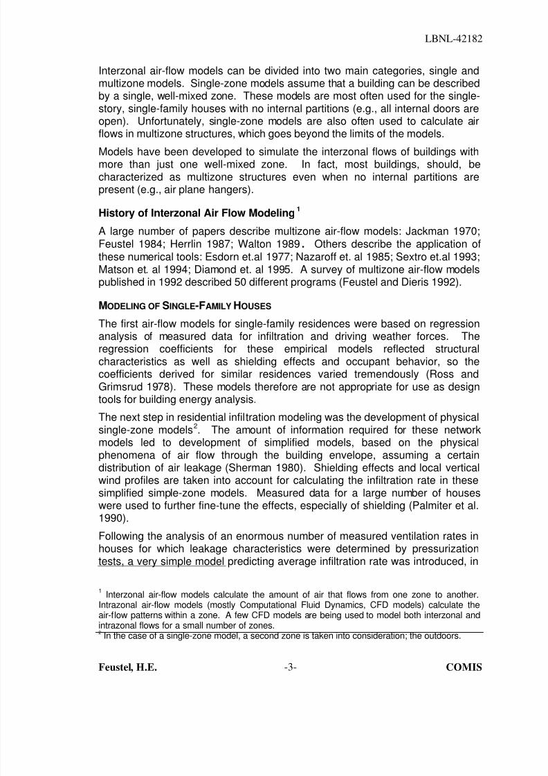
Because partitions or inhomogeneous concentration in a building create multiplezones —-areas of fully mixed volume with constant gas concentration anduniform pressure— multizone models are required to describe air flows.Multizone buildings can be single-room structures, single-family houses, or large



LBNL-42182


Figure 3: Example of a simple multizone structure (Liddament 1986)

Wind VelocityWind Direction

TemperatureDifferences

Mechanical VentilationSystems

Surroundings

Shape of the Building

Wind PressureDistribution

Vertical FlowResistance

Thermal Buoyancy

Fan and DuctCharacterist ics

Imposed Pressure

Building

Leakage Configuration

Inside PressureDistribution

Air Flow Distribution

Inhabitant Behaviour

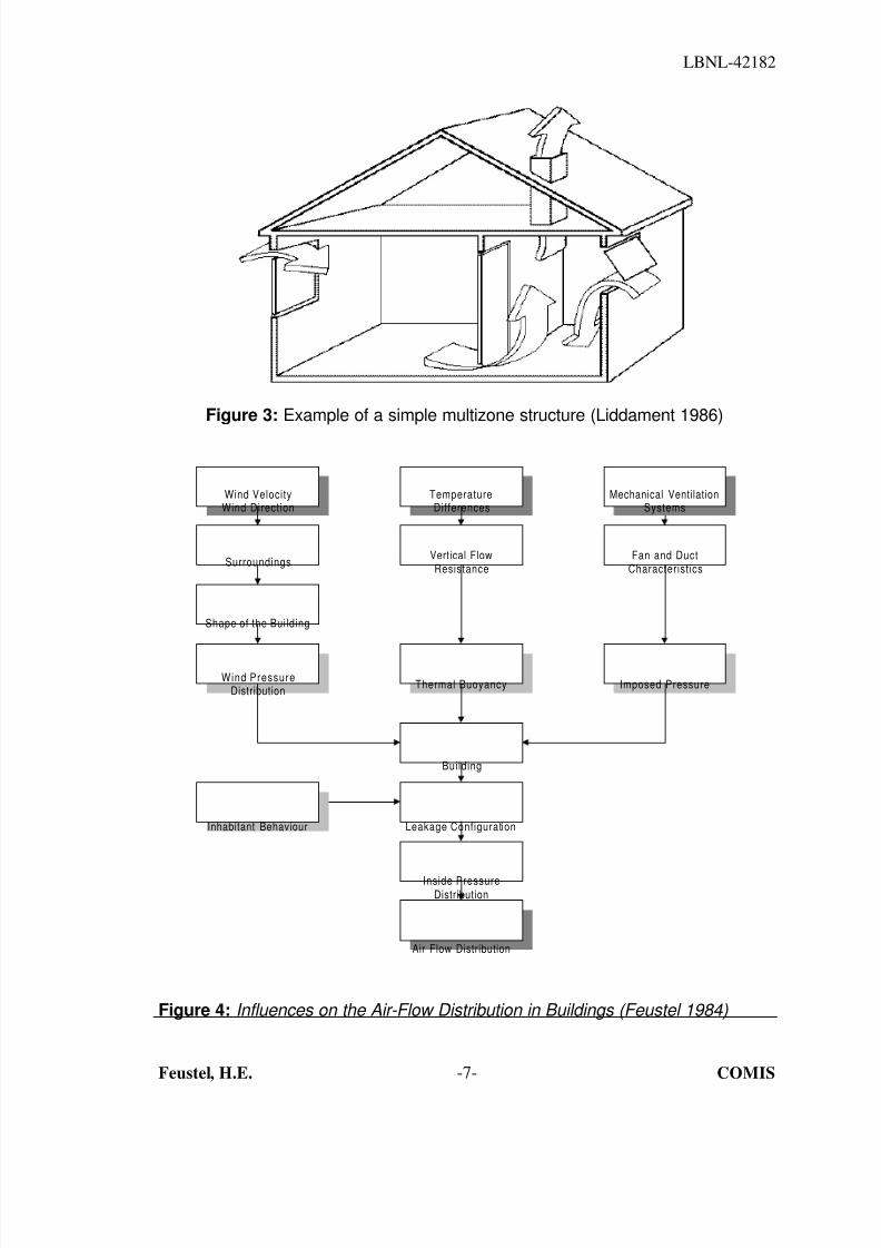
Figure 4: Influences on the Air-Flow Distribution in Buildings (Feustel 1984)



LBNL-42182


building complexes. Figure 3 shows an example of a very simple multizonebuilding.

The air flows and distribution in a given building are caused by pressuredifferences resulting from wind, thermal buoyancy, mechanical ventilationsystems, or a combination of these. Air flow is also influenced by the distributionof openings in a building’s shell and by the building’s inner pathways. Actionsby building occupants can also lead to significant differences in pressuredistribution inside a building (see Figure 4). All of these influences on air flowpatterns must be accounted for in an effective model.

Boundary Conditions

WIND PRESSURE DISTRIBUTION

The wind produces a velocity and pressure field around a building. Therelationship between velocity and the pressures at different locations in the flow

field can be obtained by analyzing the dynamics of a particle in fluid. Whencompared to the static pressure associated with an undisturbed wind-velocitypattern, the pressure field around a building is generally characterized byregions of overpressure (decrease in velocity) on the windward side, andunderpressure on the facades parallel to the air stream and on the leeward side.

The pressure distribution around a building is usually described bydimensionless pressure coefficients—the ratio of the surface pressure and thedynamic pressure to the undisturbed flow pattern:

c x y zp x y z p z

p z p

o

dyn

( , , )( , , ) ( )

( )

=−

with

p z z v zdyn out ( ) ( ) ( )=1

2

2ρ

wherec x y z p ( , , ) = pressure coefficient at coordinates x, y, z [-],

p x y z( , , ) = surface pressure at coordinates x, y, z [Pa], p zo ( ) = atmospheric pressure at height z [Pa],

p zdyn ( ) = dynamic pressure in the undisturbed flow at height z [Pa],

ρ out z( ) = density of outside air at height z [kg/m3], and

v z2 ( ) = wind speed at height z [m/s].

Figure 5 shows the air flow patterns for an isolated building with wind flowingperpendicular to the longer facade. This figure shows how complicated thedescription of the pressure field around a building can be.



LBNL-42182


Figure 5: Air flow around an isolated building

Figure 6a: Simplified wind pressure distribution; wind direction perpendicular to surface

Figure 6b: Simplified wind pressure distribution; wind direction 45

degrees



LBNL-42182


Figure 6 shows the simplified horizontal wind pressure distribution for two winddirections; wind direction perpendicular to surface and 45 degrees.

The vertical profile of a graph of wind speed in the atmospheric boundary layerdepends primarily on atmospheric stability, the roughness of terrain, thesurfaces surrounding the building i.e., the ground and/or other buildings, andwind speed increases with increasing height above ground (see Figure 7). Awind velocity profile can be approximated either by a logarithmic equation or apower law expression. The latter is most often used by engineers and buildingscientists:

v z v zz

z( ) ( )=

0

0

α

where

v z( ) = wind speed at height z [m/s],v z( )0 = wind speed at reference height z 0 [m/s], andα = exponent.

These equations assume that wind flow is isothermal and horizontal and that itwill not change direction as a result of differences in terrain. In other words,wind velocity profile is determined by the roughness of the terrain. The value ofthe exponent α increases with increasing roughness of the solid boundary. Forsmaller areas of rough surfaces in smoother surroundings, such as a townlocated in flat, open country, the velocity profile described by the equation aboveis valid only for a limited height above the obstacles.



LBNL-42182


Figure 7: Wind velocity profiles as a function of terrain (ASHRAE 1989)

Table 1: Height of boundary layer and exponents for different terrain (Davenport 1960)

roughness type height of boundarylayer [m]

exponent α [-]

flat open country 270 1/7.0 = 0.14rolling hills 390 1/3.5 = 0.28inner city areas 510 1/2.5 = 0.40

Both full-scale and wind tunnel measurements have been performed todetermine pressure distributions around buildings; results have been publishedby several authors. Hussain and Lee (1980), for example published a collectionof pressure coefficients for the vertical distribution on the center line of multistorybuildings. In general, pressure coefficients as a function of height are either“S-shaped” or “reverse C-shaped,” both of which can be described by higherorder polynomial functions (Kula and Feustel 1988).

These findings regarding pressure distribution are the basis of Grosso’s work onthe mathematical description of pressure coefficients (Grosso 1992). Based onthis work, a module calculating pressure coefficients was integrated into COMIN,the first interface developed for COMIS.

If the physical interrelationship between flow resistance and air flow is known forall flow paths, the interior air-flow distribution for a building can be calculated, aslong as there is no temperature difference between inside and outside air.



LBNL-42182


THERMAL BUOYANCY

Temperature differences between inside and outside air create air densitydifferences that cause pressure gradients. Stack-effect pressure gradientsdepend only upon temperature differences and the vertical dimension of the

building or structure (Tamura and Wilson 1967; Esdorn 1958). This effect isoften misunderstood to be a form of convection; however, temperaturedifferences within two columns of air do not cause this phenomenon; the effect isa result of the weight difference between two adjacent columns of air.

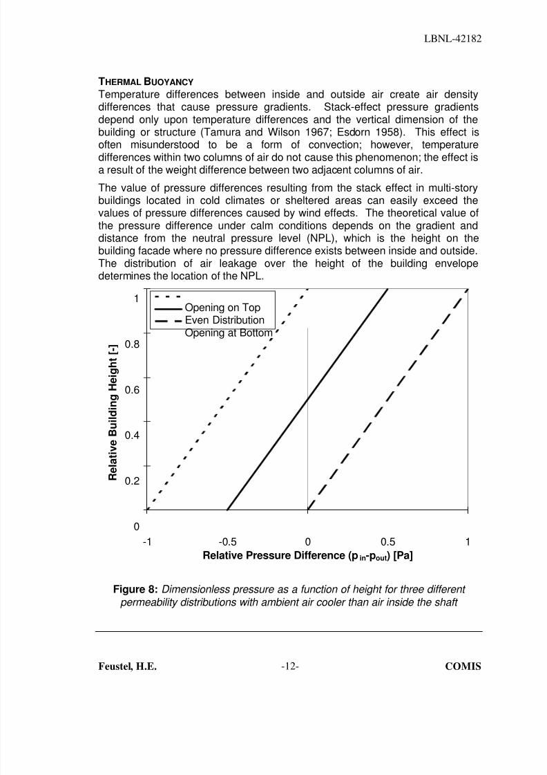
The value of pressure differences resulting from the stack effect in multi-storybuildings located in cold climates or sheltered areas can easily exceed thevalues of pressure differences caused by wind effects. The theoretical value ofthe pressure difference under calm conditions depends on the gradient anddistance from the neutral pressure level (NPL), which is the height on thebuilding facade where no pressure difference exists between inside and outside.The distribution of air leakage over the height of the building envelopedetermines the location of the NPL.

0

0.2

0.4

0.6

0.8

1

-1 -0.5 0 0.5 1Relative Pressure Difference (pin-pout) [Pa]

R e l a t i v e B u i l d i n g

H e i g h t [ - ]

Opening on TopEven DistributionOpening at Bottom

Figure 8: Dimensionless pressure as a function of height for three different permeability distributions with ambient air cooler than air inside the shaft



LBNL-42182


Figure 8 shows the pressure distribution resulting from the stack effect for threedifferent opening situations in winter i.e., when ambient temperature cooler thanair temperature inside the building shaft. If all the leakage is located at the topof the building shaft, the pressure difference on the top is zero and the bottomexperiences the maximum negative pressure difference between inside and

outside. If all the leakage is concentrated at the bottom of the shaft, thepressure difference at the bottom of the shaft is zero, and the top experiencesmaximum overpressure. If leakage occurs in the middle of the shaft or is evenlydistributed over the height of the shaft, the neutral pressure zone is in the middleof the shaft. The top experiences an overpressure, and the bottom experiencesan underpressure of the same magnitude.

The stack effect (or thermal buoyancy) can be calculated by integratingBernoulli's equation, assuming no wind:

( ) ( )( ) p p g z nplout in stack in out − = − −ρ ρ

where( ) p pout in stack

− = pressure difference due to stack effect [Pa],

g = constant of gravity [m/s2],

( )ρ ρ in out − = density difference between outside and inside air column [kg/m3],

and( ) z npl− = distance between height z and neutral pressure level [m].

MECHANICAL VENTILATION

Mechanical ventilation can be included in this flow network by treating the ductsystem like the other flow paths in the building. The fan can be described as thesource of pressure differences, lifting the pressure level between two jointsaccording to the fan’s characteristic curve (Feustel and Esdorn 1982).

Air Flow Components

CRACK FLOW

The one air-flow component covered by all air flow models found in the reviewprocess (Feustel and Kendon 1985; Feustel and Dieris 1992) is the crack. Airflow through a crack is always a mixture of laminar, turbulent, and transition flow.

The proportion of each depends on the shape of the crack and the pressuredifference on either side of the crack.

The power law equation is widely used to express the air flow characteristics ofcracks:

Q C PQ

n= ( )∆ .



LBNL-42182


This numerical representation is simple and meaningful. It shows that the airflow Q depends on the pressure difference ∆P ; however, this equation does nottake into account the influence of the air properties and the air-flow rate.Correction factors to account for these influences were introduced to the simplepower law equation in the COMIS Fundamentals (Feustel and Raynor-

Hooson1990).The classification of cracks helps to determine the correction factors and todetermine the air leakage coefficient C Q and the pressure exponent n . Cracks

are either classified according to their component type or their physical behavior.As the types of cracks in a specific building are usually not known, the lattermethod is not practical for air leakage calculations for real buildings.

In air-flow simulations, building components (e.g., windows, walls, closed doors)are often treated as single leakages. This has the advantage of reducing theinput requirement, but reduces the accuracy of the simulation result because theair-flow is represented by only one set of boundary conditions (e.g., thermalgradients over the height of the component are neglected).

FLOW THROUGH VERTICAL LARGE OPENINGS

Air flow through large openings (e.g., open doorways or open windows) is amain contributor to the transfer of air, pollutants and thermal energy from onezone of a building to another zone or to the outside. In most circumstances,thermal differences and/or differences in thermal gradients on both sides of alarge opening will cause two-way flows. The prediction of air flows through largeopenings is difficult. Although good agreement exists in the literature regardingprediction of gravitational flows through large openings in steady-stateconditions, large uncertainty remains regarding the definition of the dischargecoefficient (Allard and Utsumi 1992).

Air flow through large openings involves a number of different physicalphenomena, including steady-state gravitational flows, fluctuating flows resultingfrom wind turbulence, and recirculation flows caused by boundary layer effectsin a thermally driven opening (Allard and Utsumi 1992). The general descriptionof gravitational air flow through a vertical opening is shown in Figure 9. Allardand Utsumi show that a large vertical opening can have two, one, or zero neutralpressure levels. For large openings inside buildings, we most often find oneneutral pressure level close to the middle of the opening’s height.

For large openings incorporated COMIS calculates the mass flow and itsderivative for both flow directions. Density profiles in neighboring zones arerepresented by pressure or density values at the bottom and top of the openingand at several levels spaced equal distances apart within the opening. Themass flow is calculated for each level. The total flow is obtained by summationof the flows for the whole opening (Dorer 1995). The air flows can be calculatedfor the following cases:



LBNL-42182


• closed large opening: In this case, the air flows from the cracks at thebottom and top of the component is calculated according to their pressuredifferences. The air flow for the vertical cracks is calculated by thesummation of the flows over the vertical height.

• normal rectangular vertical openings: The calculation procedure described

above is used. The discharge coefficient, which takes into account thecontraction of the flow resulting from the existence of the opening, can beeither defined by the user or calculated by COMIS.

• horizontally pivoted window: The flow direction is assumed to beperpendicular to the plane of the opening; the air flow is integrated over thevertical dimension of the window.

t 0P

0

ρρρρ

ρρ

zt+bt(z) = PtP Z

02P

0201

1

2

ZN

ZN

O

g

H

P01

1(z) =

01+b

1z

z2

+b02

(z) =2

Figure 9: Description of the general problem of gravitational flow through vertical large openings; Index 0 = Reference Height, Index 1 = Zone 1, Index 2 = Zone 2,

Index t = effect of turbulence (Alllard and Utsumi 1992)

COMIS also includes a routine to calculate bouyancy-driven air flow throughsingle-sided ventilation (van der Maas 1992). This is the only case where thechanging thermal properties of a room are taken into account. The driving factorhere is a temperature difference between the room and the outside. When a

window is open, the room air temperature is being calculated as a function of theinitial temperatures specified by the user, the thermal properties of the zoneenvelope, and the length of time during which the window is open.

Window opening angle can be calculated based on the weather data (outdoorair temperature and wind velocity).

The simulation of large vertical openings in a building’s facade was evaluated bya team of scientists from Belgium, France, and Greece (Dascalaki et. al 1998)



LBNL-42182


for single-sided ventilation and cross-flow ventilation. For single-sidedventilation at low wind speeds, COMIS predicts the air flows with satisfactoryaccuracy relative to the measured data. The cross-flow experiments performedat low wind speeds also show good agreement with COMIS’ results. However,Dascalaki et. al. report that inaccuracies in pressure and discharge coefficients

may cause significant errors in estimating air flows between the outside andinternal zones.

DUCTS

Pressure losses through duct work are calculated based on friction lossesdescribed by Moody (1944) and dynamic losses resulting from flow disturbancescaused by fittings that change the path and/or area of air flow:

∆ ∆ ∆P P Ploss friction fittings= +

∆Pl

d P friction dynamic= λ

where

∆P friction = friction losses in the duct [Pa],

λ = dimensionless friction factor [-], l = length of the duct [m], d = diameter of the duct [m], and Pdynamic = dynamic pressure of the air flow [Pa].

Within the region of laminar flow (Reynolds number less than 2,000), the frictionis a function of the Reynolds number only, and can be written as:

λ = 64Re

where

Re = dimensionless Reynolds number [-].

For turbulent flow (Reynolds numbers greater than 10,000), the friction factordepends on the Reynolds number, duct surface roughness, and internalprotuberances (such as joints) and is calculated by Colebrook’s equation:

1

2375

251

λ

ε λ = − +

log.

.

Red

where

ε surface roughness [m].

Because this equation cannot be solved explicitly for λ , we use an approximateexplicit equation from Moody (1944):



LBNL-42182


λ ε

= + +

1 20000

106 1/3

d Re.

Dynamic losses due to fittings are expressed as: ∆P P fittings dynamic= ×ζ

where

ζ = dimensionless coefficient [-].

Fittings included in COMIS are entries, exits, transitions, and junctions. Thedimensionless coefficient ζ , which has the same value in dynamically similarstreams (i.e., streams with geometrically similar stretches, equal values ofReynolds number), has been obtained from engineering handbooks (ASHRAE1985; Hönmann 1987).

In COMIS, the flow through a duct is modeled as the power law function.Because friction along the duct is different for laminar, turbulent, and transitionalregions, the flow coefficient C Q and the exponent n are calculated by means of

iteration (Feustel and Raynor-Hoosen 1990). Because of the nonlinearinterdependency of flows in the branches of a junction, duct work with manyfunctions requires more iterations. A flow path in which resistance is dominatedby pressure drops in the junction might make a system unstable.

PASSIVE STACKS

A passive stack component of COMIS was developed in response to the request

of IEA-ECB’s Annex 27 “Residential Ventilation Systems”3

A passive stack forms a link from a building zone to the outside (roof) andincludes the following elements:• a grille or opening, visible in the room, mounted on the duct;• a duct, which is round or rectangular; and• a cowl (hood) at the top of the duct outside.

The pressure loss for the passive stack is defined as follows:

( )∆P

q

A

q

A

L

D

q

q v Cpv

grille

v

duct

v out

meteo cowl=

+

+

+ −

ρ λ

ζ

ρ

2 2

2 2

1

2

.. .

where

qv = flow through the vertical duct [m3 /s],

3 IEA-ECB: International Energy Agency, Energy Conservation in Buildings and CommunitySystems program



LBNL-42182


q1 = flow at cowl at 1 Pa [m3 /s],

Agrille = free flow area of the grille [m2],

Aduct = free flow area of the duct [m2],

vmeteo = velocity at roof height [m/s], and

Cpcowl = pressure coefficient resulting from cowl [-].

The last term accounts for the extra pressure loss resulting from the presence ofthe cowl. “ q

1” The flow through the cowl at the pressure of 1Pa is q

1, calculated

as follows:

q Aduct 1

2=

ρζ .

FANS

Fans are a source of pressure differences, lifting the pressure level between twozones. In COMIS, fans are described by the polynomial fan curve eitherprovided by the user or approximated by COMIS from a set of volumeflow/pressure data pairs. In order to avoid unstable fan performance in themodel, the flow/pressure relationship outside the range given by data pairs isassumed to be of linear character (see Figure 10).

mF

Third order polynomialapproximation

Real

Flow

PmaxPmin

mF = Slope * p + Intercept

Linear extrapolation

Pressure p

Figure 10: Fan curve approximation using coefficients (Feustel and Smith 1998)



LBNL-42182


Flow through the fan is calculated for deviating values of fan speed or air densityaccording to fan laws. Fan speed can be changed by means of a fan schedule,which allows a change of fan speed to change at any time during the simulationperiod.

Outside the specified range of fan performance, a linear approximation is used

to ensure that the network solver will find a valid solution and not become stuckoutside the correctly approximated curve.

FLOW CONTROLLERS

Four types of flow controllers are distinguished; these four, represent most of theavailable dampers or regulators that respond to pressure drop or (duct) flow.Controllers with temperatures as input must be simulated with the schedules,which is not an ideal modeling solution.

The basic premise of controllers is that they have an opening through which theair flows. At higher pressures, a flap or valve may throttle the flow by graduallyclosing the opening. The flow controllers' performance is divided into threepressure ranges (see Feustel and Smith 1998).

Range 1:At low pressures the controller is fully open and not blocked by either flap orvalve. This position is simulated with a normal crack flow equation.

Range 2:Above a certain pressure, a moving flap or valve will decrease the controller’sopening, limiting the flow or keeping it roughly constant. This position issimulated either by a single constant flow rate or with a curve approximated by apolynomial. The transition point between range 1 and range 2 is simply definedin the program by the intersection of the two curves. This curve or constant flowwill be maintained until it intersects with the curve from range 3.



LBNL-42182


-0.5

-0.4

-0.3

-0.2

-0.1

0

0.1

0.2

0.3

0.4

0.5

-5 -4 -3 -2 -1 0 1 2 3 4 5Dp [Pa]

F l o w [ k

g / s ]

Facade LeakageFlow ControllerComponent F1 (Flow Controller + Facade Leakage)

Range 1 Range 2

Setpoint

Figure 11: Performance of flow controller (F1 = ideal symmetrical) (Feustel and Smith 1998)

Range 3:At high pressures the controller flap or valve may:-close no further or have leaks-close faster, reducing the flow at increasing pressure to almost zero.

Like range 2, range 3 is simulated with a polynomial.There are four different flow controllers in COMIS; each of them provides adifferent air flow performance as a function of pressure difference. Figure 11shows the performance of an ideal symmetrical flow controller in conjunction withfaçade leakage.

Kitchen HoodCOMIS models kitchen hoods in different ways. Kitchen hoods can be either fanoperated or stack operated. The hood itself can be simulated by means of a setof power law equations (i.e., by using the crack component) or by using a

component that calculates the spread of pollutants into the zone (see Figure12).



LBNL-42182


Figure 12: Schematics of Kitchen Hoods as modeled in COMIS (Phaff 1996)(Numbers 1,2,3 and 4 are flow paths between zones.)

In the latter case, the spread of pollutants will be calculated using spreadcharacteristics as a function of the exhaust flow of the hood. The spreadcharacteristics (hood efficiency) must be provided by the user. These data areoften available from kitchen hood manufacturers (Feustel and Smith 1998).

USER-DEFINED AIR-FLOW COMPONENTS

COMIS allows the user to define air-flow components. The characteristics ofthese components need to be provided in terms of data pairs describing theflow/pressure relationship. With this air-flow components that are not standardlyincluded in the program can thus be added.

Other Program Features

TIME STEP

A time step is the period between events during a simulation. Simulations areperformed for a time period defined by a start and stop time provided by theuser. COMIS works with two different time steps: one for the air-flowcalculations and another for calculation of pollutant transport. As air flows arequasi-steady-state phenomena, the time step used for air-flow calculations is



LBNL-42182


based only on “external events,” which are schedules provided by the user. Thetime step is determined by the change of boundary conditions with time, i.e.,weather data, opening configuration, fan schedule, etc.

Pollutant transport and the related buildup or decay of contaminantconcentrations are not steady-state physical phenomena. Therefore, the time

step is calculated based on the shortest time constant of all zones within abuilding for a particular simulation configuration (Feustel and Raynor-Hooson1990).

ZONE LAYERS

A zone can be divided vertically into several sub-zones (layers). Layers allowfor zones with more than one gradient for zone temperature and/or humidity(e.g., shafts, staircases). Layers may also be used to account for differentsources or sinks in different heights of a zone. There is no limit to the number oflayers that can be specified in a zone.

SCHEDULES

A series of events for a particular parameter are described by schedules.Schedules describe the time of an event and the event itself. COMIS providesthe following options for schedules:

weather data (wind velocity, wind direction, air temperature, absolutehumidity, barometric pressure), window schedule (window openingfraction), fan schedule (fan speed factor), zone temperature, absolutehumidity, sink schedule (for up to five pollutants), source for (up to fivepollutants), multi-schedule (for up to ten parameters with a common timestep).

The time steps for all these schedules can be variable, ranging from a second tothe length of the simulation period. Schedules can either be included in theCOMIS input file or provided by separate schedule files. In the latter case, theCOMIS input file only contains the name(s) of the schedule file(s).

CONTAMINANT TRANSPORT

Besides calculating air flow between zones, COMIS also calculates the transportand distribution of up to five contaminants. Simulation of contaminant transportin a multizone building leads to the definition of mass balance equations foreach pollutant considered in each zone, based on the assumption that thepollutant concentration is well mixed in a zone and is transported from zone to

zone by the flow of air. COMIS allows for filter effects for all air-flowcomponents; these effects can represent a solid absorption along the path orany kind of reaction (chemical reaction, phase change, etc.) resulting fromcontact of the pollutant with a solid material as it flows from one zone to another(Feustel and Smith 1990).

Although the air flow in buildings can be assumed to be steady state,contaminant transport is a dynamic effect. Therefore, it is critical to use a time



LBNL-42182


step short enough to represent the dynamics. COMIS calculates the time stepfor contaminant transport as a function of the shortest time constant of all zonesconsidered. Therefore, the critical zone in a building for this calculation willhave a small volume but a high air flow. When duct work is realisticallysimulated, this critical zone is often part of the duct work.

OUTPUT OPTIONS

COMIS provides a variety of output options. Besides the basic option, whichprovides air-flow and pollutant transport data for each time step, data can berecorded or calculated in the form of tables. Calculations include the air changerates for individual zones and/or the whole building, mean age of air, the airchange efficiency of the building, and the room air change index. It is alsopossible to have mean values for the whole simulation period being calculatedand reported (Dorer and Weber 1995).

The ventilation heat loss energy, based on the incoming air temperature and thetemperature difference between inside and outside of the building, is alsocalculated. For zones with temperature gradients, the temperature at the link isconsidered.

USER INTERFACE

Several interfaces were developed for COMIS. The simplest is the FORTRANprogram COMIN. This program reads and writes COMIS input files and allowsthe addition, change, and deletion of input data. COMIN is hardware-independent but bothersome to work with, so other interfaces, COMERL, llSiBatand XCOMIS were developed.

COMERL offers an alphanumeric, DOS™-oriented user interface allowing the

creation or modification of COMIS input files using a specific task-adaptededitor. A data base for air flow components (e.g., cracks, windows, HVACcomponents) is integrated into COMERL. The pre- and post-processorprograms COMIN and COMOUT as well as the simulation program COMIS canbe run from within the shell (Dorer et al. 1995).

IISiBat is the Intelligent Simulation Environment (ISE) graphics interface adaptedfor COMIS. It provides a sophisticated graphical environment that runs on PCsor workstations and allows the user to enter information in a straightforward way.IISiBat provides both inexperienced and advanced users with tools that cancalculate the dynamics of complex systems.

The ISE allows sharing of data between various simulation tools and coupling ofsimulation tools; it also includes built-in checking and helping functions. IISiBatincludes the model documentation in the standard format PROFORMA (Pelletretet al. 1992).



LBNL-42182


Figure 13: IISiBat model library (Keilholz 1997)

Components and projects are stored in object-oriented libraries. Air-flowcomponents are arranged in a “tree structure,” as illustrated for duct fittings inFigure 13. When a family of components (e.g., duct fittings) is selected, the tree

develops to show various component types. Physical properties are attached toeach component. Figure 14 shows an air-flow network with the boundaryconditions as developed with IISiBat.



LBNL-42182


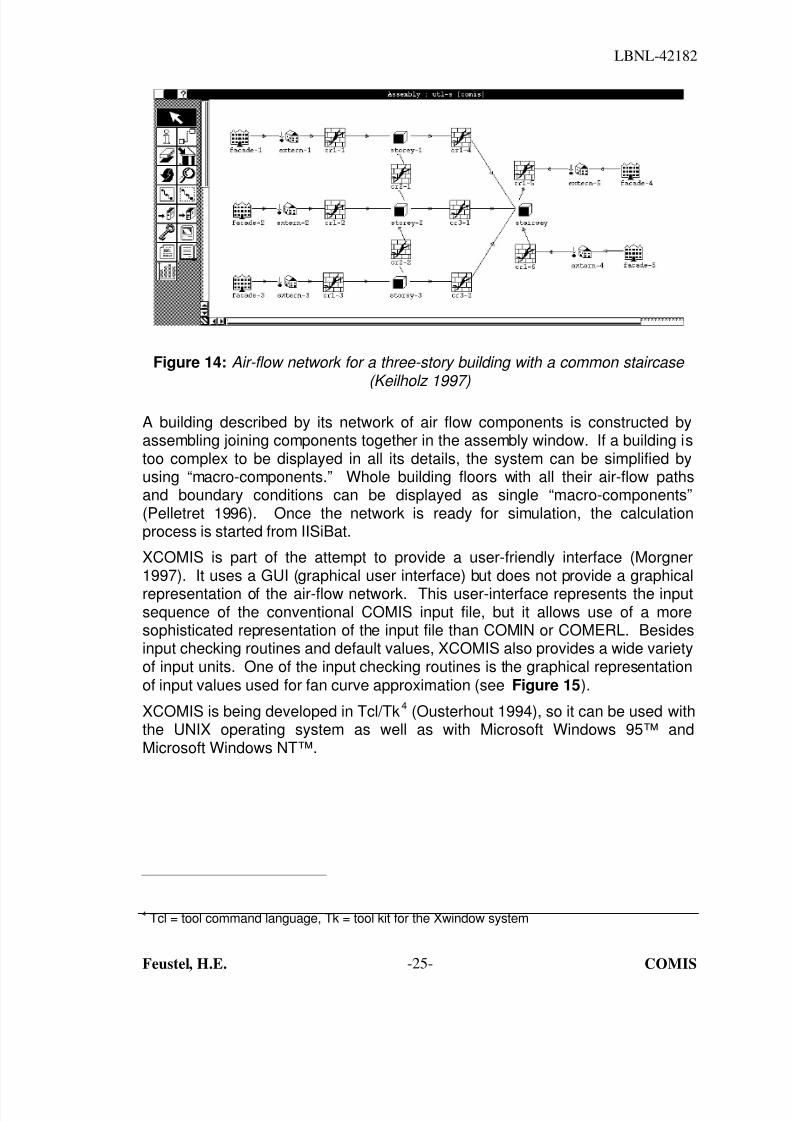
Figure 14: Air-flow network for a three-story building with a common staircase (Keilholz 1997)

A building described by its network of air flow components is constructed byassembling joining components together in the assembly window. If a building istoo complex to be displayed in all its details, the system can be simplified byusing “macro-components.” Whole building floors with all their air-flow pathsand boundary conditions can be displayed as single “macro-components”(Pelletret 1996). Once the network is ready for simulation, the calculationprocess is started from IISiBat.

XCOMIS is part of the attempt to provide a user-friendly interface (Morgner1997). It uses a GUI (graphical user interface) but does not provide a graphical

representation of the air-flow network. This user-interface represents the inputsequence of the conventional COMIS input file, but it allows use of a moresophisticated representation of the input file than COMIN or COMERL. Besidesinput checking routines and default values, XCOMIS also provides a wide varietyof input units. One of the input checking routines is the graphical representationof input values used for fan curve approximation (see Figure 15).

XCOMIS is being developed in Tcl/Tk4 (Ousterhout 1994), so it can be used withthe UNIX operating system as well as with Microsoft Windows 95™ andMicrosoft Windows NT™.

4 Tcl = tool command language, Tk = tool kit for the Xwindow system



LBNL-42182


Figure 15: XCOMIS graphic tool for fan curve approximation (Morgner 1997)

Evaluation of Multizone Air-Flow ModelsThere is a lack of measured infiltration and ventilation data for whole buildings.These data are essential for validating air-flow models. Critical variables mustbe identified for different building types in order to develop more accurate inputdata and, ultimately, more accurate models. Wind pressure coefficients, forexample, need further study; the collating of existing data could help our efforts

in simplifying data requirements.The difficulty of measuring infiltration in buildings under controlled boundaryconditions means that none of the multizone models has been validatedproperly, if at all (Scartezzini et. al 1987). The possibility of doing piecemealvalidations of certain algorithms has been considered (e.g., the algorithms for airflow through open doorways or air flow through cracks). Measuring a few zonesof the whole structure would effectively test existing models. However,validation of a model’s performance for whole buildings is preferable, as wasdone for COMIS.

The goal of the IEA’s Annex 235 was to provide a reliable, accurate, practical,

and user-friendly multizone air flow model. A variety of tests were performed tomake sure that COMIS contains no numerical errors; COMIS simulation resultswere compared with more than 50 benchmarks for which either an analytical or anumerical solution was obtained. Each of these test cases was developed tocheck a particular feature of the program. These tests were repeated for each

5 International Energy Agency’s Energy Conservation in Buildings and Community Systemsimplementing agreement, Annex 23 “Multizone Air Flow Modeling”



LBNL-42182


individual program update to be sure that a model improvement did not interferewith already tested program features.

Furthermore, two user tests were developed as a joint contribution by the AirInfiltration and Ventilation Centre and researchers in Switzerland. The first testrepresents a very simple network in which all openings and pressure boundary

conditions are defined. This test and the comparison of simulation results withanalytical solutions enabled inconsistencies and problems in the code to bequickly identified and rectified.

A second test was performed to evaluate the influence, of the user on theprogram’s accuracy. This test helped us to develop the program documentation,particularly the User’s Guide. The results showed clearly that the user’s ability iscritical in securing reliable predictions (Liddament 1996).

COMIS was also checked by means of model intercomparison (Fürbringer et. al1996). Fourteen other simulation programs6 were used by the research groupsinvolved in evaluating COMIS, and results were compared. Because differentprograms have different features, the objectives for each intercomparison had tobe adapted so that the models to be compared could simulate the same physicalphenomenon. Because all programs use similar algorithms, and simulationswere performed with identical input data, so the results fall within a very narrowband.

The comparison of results between the model and in-situ tests was an importantpart of the work done to develop COMIS. Nine studies were performed, usingresults from tracer gas tests for single-family houses, test cells, flats, and smalloffice buildings. These results were compared with results obtained bynumerical simulation. For each case, a sensitivity analysis was performed, not

only to learn about the uncertainties in the measurements but also about theconfidence intervals of the simulations, which result from uncertainties in theinput data (Fürbringer et. al. 1996).

How to Obtain IISiBat/COMISCOMIS and its user interface IISiBat together with all the necessary user’sguides can be downloaded for free using the following world wide web address:

http://www-epb.lbl.gov/comis/

ConclusionsUser-friendliness and confidence in a model are prerequisites for its use. Annex23 was adopted by the International Energy Agency to work specifically towardsthis goal. The ISE user interface developed for COMIS is a significant steptowards "user-friendliness." IISiBat provides a graphical representation of thenodal model with all the boundary conditions and air flow components in use.

6 Models compared include AIDA, AIRNET, ASCOS, BREEZE, BREVENT, CBSAIR,CONTAM93, ESP, LBL, MZAP, NORMA, PASSPORT AIR, TURBUL, and VENCON.



LBNL-42182


Additionally, IISiBat functions as a program shell; simulations and outputrepresentation can be controlled from within the interface.

A significant effort was made towards the evaluation of the model. Besidesbenchmark testing, and model intercomparison, in-situ measurement exerciseswere performed for several building structures. With this effort, COMIS is

probably the only multizone air flow model which has been evaluated at differentlevels.

The international authorship and the efforts to maintain the program in the futurehave helped to establish COMIS as a standard for air flow/pollutant transportmodels.

Future developments include the coupling of COMIS with the thermal buildingsimulation model EnergyPlus and the incorporation of the aerosol/particledeposition model for rooms. A zonal model currently developed at ConcordiaUniversity will also be included into COMIS.

AcknowledgmentsThis report was supported by the Assistant Secretary for Energy Efficiency andRenewable Energy, Office of Building Technology, of the U.S. Department ofEnergy under Contract No. DE-AC03-76SF00098.

ReferencesAIVC TN 31, 1991. “Air Flow Patterns: Measurement Techniques,” Air Infiltrationand Ventilation Centre

ASHRAE 1985. Handbook of Fundamentals , Chapter 22, American Society ofHeating, Refrigerating and Air-Conditioning Engineers, Atlanta, GA

ASHRAE 1989. Handbook of Fundamentals , Chapter 14, American Society ofHeating, Refrigerating and Air-Conditioning Engineers, Atlanta, GA

DIN 4701, 1983. “Regeln für die Berechnung des Wärmebedarfs von Gebäuden,Teil 1: Grundlagen der Berechnung,” Beuth Vertrieb Berlin

Allard F., and Y. Utsumi, 1992. “Air Flow through Large Openings,” Energy and Buildings , 18, 133-145

Davenport, A.G., 1960. “A Rational for the Determination of Basic Design WindVelocities,” ASCE-Proceedings, Vol. 86, 36 -68

Diamond, R.C., and H.E. Feustel, 1995. “Ventilation in High-Rise Residential

Buildings,” In Proceedings, 16th Air Infiltration and Ventilation Conference , PalmSprings, CA

Dascalaki, E., M. Santamouris, M. Bruant, C.A. Balaras, A. Bossaer, D.Ducarme, and P. Wouters, 1998. “Modeling Large Openings with COMIS,”Energy and Buildings, same Volume

Dorer, V., 1995. “New Large Vertical Opening and Single-Sided VentilationRoutines in COMIS,” Internal Annex Report, EMPA Dübendorf



LBNL-42182


Dorer, V. and A. Weber, 1995. “Output Options for COMIS,” Internal AnnexReport, EMPA Dübendorf

Dorer, V., F. Huck, and A. Weber, 1995. "COMERL PC-based User Interface forthe Multizone Air Flow and Contaminant Transport Model COMIS,” EMPADübendorf

Esdorn, H., 1958. “Luftdurchlässigkeit der Fenster und Druckverteilung imGebäude,” Das Hochhaus der BASF, Planung, Ausführung, Erfahrungen , J.Hoffmann, Stuttgart

Esdorn, H., H.E. Feustel, K. Giese, and M. Schmidt, 1977. “Bauliche undlüftungstechnische Maßnahmen gegen unerwünschten Luftaustausch zwischenRäumen unterschiedlichen hygienischen Standards,” Schlußbericht TP F2/2,Sonderforschungsbereich 159, Krankenhausbau, Technische Universität Berlin

Feustel, H.E., 1996. “Annex 23 - An International Effort in Multizone Air FlowModeling,” In Proceedings, ROOMVENT ‘96 , Yokohama

Feustel, H.E., 1984 “Beitrag zur theoretischen Beschreibung der Druck- undLuftmassenstromverteilung in natürlich und maschinell gelüfteten Gebäuden,”Fortschritt-Berichte der VDI Zeitschriften , Reihe 6, Nr. 151, VDI Verlag,Düsseldorf

Feustel, H.E., A. de Almeida, and C. Blumstein, 1992. “Alternatives toCompressor Cooling in Residences,” Energy and Buildings , Vol. 18, No. 3-4

Feustel, H.E., F. Allard, V.B. Dorer, M. Grosso, M. Herrlin, M. Liu, J.C. Phaff, Y.Utsumi, and H. Yoshino, 1989. "The COMIS Infiltration Model,” in Proceedings,Building Simulation '89 , The International Building Performance SimulationAssociation, Vancouver

Feustel, H.E. and V.M. Kendon, 1985. "Infiltration Models for MulticellularStructures,” Energy and Buildings, Vol. 8, No. 2

Feustel, H.E., H. Esdorn, 1982. “Mass Flow Distribution in High-Rise Buildingswith Forced Ventilation Systems,” In Proceedings, International Conference on System Simulation in Buildings , Liege

Feustel, H.E. and J. Dieris, 1992. "A Survey on Air Flow Models for MultizoneStructures,” Energy and Buildings , Vol. 18

Feustel, H.E., and A. Raynor-Hooson (Editors), 1990. “COMIS Fundamentals,”Air Infiltration and Ventilation Centre, Technical Note 29, Lawrence Berkeley

Laboratory Report, LBL-28560Feustel, H. E., and M.H. Sherman, 1989. “A Simplified Model for Predicting AirFlow in Multizone Structures,” Energy and Buildings , Vol. 13, No. 3, LawrenceBerkeley Laboratory Report, LBL-22325

Feustel, H.E., and B.V. Smith (Editors), 1998. “COMIS 3.0 User’s Guide,”http://www-epb.lbl.gov/comis/



LBNL-42182


Fürbringer, J.M., C.-A. Roulet, and R. Borchiellini, 1996. "Annex 23 SubtaskII&III Report - Evaluation of COMIS,” Vol. 1 and Vol. 2, EPFL Lausanne,Switzerland

Grosso, M., 1992. “Wind Pressure Distribution around Buildings; a parametricalModel,” Energy and Buildings , 18, 101-131

Herrlin, M., 1990. “Solution Methods for Air Flow Networks,” in COMISFundamentals, Lawrence Berkeley Laboratory Report, LBL-28560

Herrlin, M., 1987. “Luftstromning I byggnader - en berakningsmodell,” Division ofBuilding Services Engineering, Royal Institute of Technology, Stockholm,Sweden

Hönmann, W., 1987. “Taschenbuch für Heizung und Klimatechnik,” R.Oldenburg Verlag, München, Wien

Jackman, P. J.,1970. "A Study of Natural Ventilation of Tall Office Buildings,”Inst. Heat Vent. Eng., Vol. 38

Keilholz, W., 1997. “IISiBat/COMIS 3.0 User’s Guide,”http://evl.cstb.fr/iisibat.html

Kula, H.-G., and H.E. Feustel, 1988. “Review of Wind Pressure Distribution asInput Data for Infiltration Models,” Lawrence Berkeley Laboratory Report, LBL-23886

Liddament, M.W., 1986. "Air Infiltration Calculation Techniques - an ApplicationsGuide,” Air Infiltration and Ventilation Centre, Bracknell, U.K.

Liddament, M.W., 1996. “Two Air Flow Studies Completed,” Air Infiltration Review , Vol. 17, No. 4, Air Infiltration and Ventilation Centre, Bracknell, U.K.

Matson, N. E., H.E. Feustel, J. L. Warner und J. Talbott, 1994. “Climate-BasedAnalysis of Residential Ventilation Options: New York State Analysis,” InProceedings, 15th AIVC Conference, The Role of Ventilation , Buxton

Moody, L.F., 1944. “Friction Factors for Pipe Flow,” ASME Transactions,American Society of Mechanical Engineers, New York

Morgner, S., 1997. “XCOMIS -- Development of a Graphical User Interface forthe Multizone Air Flow and Contaminant Transport Simulation Model COMIS,”Masters Thesis, Georg-Simon-Ohm Fachhochschule, Nuremberg

Nazaroff, W., H.E. Feustel, A. Nero, K. Revzan, D.T. Grimsrud, M. Essling, and

R. Toohey, 1985. “Radon Transport into a Single-Family House with aBasement,” Atmospheric Environment , Vol. 19, No. 1, Lawrence BerkeleyLaboratory Report, LBL-16572

Ousterhout, J.K., 1994. “Tcl and the Tk Toolkit,” Addison-Wesley PublishingCompany



LBNL-42182


Palmiter, L., I. Brown, and T. Bond, 1990. “Residential ConstructionDemonstration Project Cycle II: Infiltration in New All-Electric Homes in thePacific Northwest,” Report prepared for the Washington State Energy Office

Pelletret, R., 1996. “IISiBat - A User Interface for Multizone Modelling (Annex23),” News , International Energy Agency, Energy Conservation in Buildings and

Community Systems ProgrammePelletret, R., S. Soubra, W. Keilholz, A. Melouk, 1992. "Annex 23 - Multizone AirFlow and Pollutant Transport Modeling, Subtask 1: The Multizone Air Flow andPollutant Transport Model developed in the Frame of the IEA Annex 23,” inProceedings International Symposium - Air Flow in Multizone Structures , Vol. 1,Budapest

Phaff, J.C., 1996. “Final Report Annex 23 - Multizone Ventilation Models:Participation of TNO Bouw. Examples,” TNO Report 96-BBI-R1086

Ross, H.D., and D.T. Grimsrud, 1978. “Air Infiltration in Buildings - Literature

Survey and Proposed Research Agenda,” Lawrence Berkeley LaboratoryReport, LBL-7822

Scartezzini, J.-L., J.-M. Furbringer, C.-A. Roulet, H.E. Feustel, 1987. “DataNeeds for Purpose of Air Infiltration Computer Code Validation,” In Proceedings,8th AIVC Conference, Ventilation Technology - Research and Application ,Überlingen

Sextro, R.G., H.E. Feustel, M. P. Modera, K. L. Revzan, M. H. Sherman, 1993.“A Coupled Multizone Flow and Radon Transport Model of Radon Entry andConcentrations in a Crawlspace House,” In Proceedings, Indoor Air '93 , Helsinki

Sherman, M.H., 1980. “Air Infiltration in Buildings,” Lawrence Berkeley

Laboratory Report, LBL-10712Sherman, M.H., 1995. "The Use of Blower-Door Data,” Indoor Air , Vol. 5, 215-224

Sherman, M.H. and D.J. Dickerhoff, 1994. "Air Tightness of U.S. Dwellings,” InProceedings, 15th AIVC Conference, The Role of Ventilation , Volume 1, Buxton,U.K.

Sherman, M.H., H.E. Feustel, D. J. Dickerhoff, 1991. “Description of a System forMeasuring Interzonal Air Flows Using Multiple Tracer Gasses,” In Proceedings,Heat and Mass Transfer in Building Materials and Structures , Hemisphere

Publishing Corporation, New York, Washington, Philadelphia, LondonTamura, G.T., and A.G. Wilson. “Pressur Difference caused by Chimney Effectin three high Buildings,” ASHRAE Transactions , Vol 72, Part II, II.1.1 - II.1.10

van der Mass, K., 1992. “IEA-ECB Annex 20 Technical Report: Air Flow throughLarge Openings in Buildings,” International Energy Agency



LBNL-42182

Walton, G.N., 1989. ”AIRNET - A Computer Program for Building AirflowNetwork Modeling,” United States Department of Commerce, National Institute ofStandards and Technology

Walton, G.N., 1994. “CONTAM 93 User Manual,” United States Department ofCommerce, National Institute of Standards and Technology, NISTIR 5385, 1994

An International Multizone Air-Flow and Contaminant Transport Model

Documents

Transcript of An International Multizone Air-Flow and Contaminant Transport Model