AN INTEGRAL EQUATION METHOD FOR CONFORMAL …eprints.utm.my/id/eprint/9746/1/78089.pdf ·...
160
AN INTEGRAL EQUATION METHOD FOR CONFORMAL MAPPING OF DOUBLY AND MULTIPLY CONNECTED REGION VIA THE KERZMAN-STEIN AND NEUMANN KERNELS KAEDAH PERSAMAAN KAMIRAN UNTUK PEMETAAN KONFORMAL BAGI RANTAU BERKAIT GANDA DUA DAN BERKAIT BERGANDA MELALUI INTI KERZMAN-STEIN DAN NEUMANN ALI HASSAN MOHAMED MURID HU LAEY NEE MOHD NOR MOHAMAD NURUL AKMAL MAHAMED NOR IZZATI JAINI Department of Mathematics Faculty of Science Universiti Teknologi Malaysia 2009
Transcript of AN INTEGRAL EQUATION METHOD FOR CONFORMAL …eprints.utm.my/id/eprint/9746/1/78089.pdf ·...
AN INTEGRAL EQUATION METHOD FOR CONFORMAL MAPPING
OF DOUBLY AND MULTIPLY CONNECTED REGION
VIA THE KERZMAN-STEIN AND NEUMANN KERNELS
KAEDAH PERSAMAAN KAMIRAN UNTUK PEMETAAN KONFORMAL
BAGI RANTAU BERKAIT GANDA DUA DAN BERKAIT BERGANDA
MELALUI INTI KERZMAN-STEIN DAN NEUMANN
ALI HASSAN MOHAMED MURID
HU LAEY NEE
MOHD NOR MOHAMAD
NURUL AKMAL MAHAMED
NOR IZZATI JAINI
Department of Mathematics
Faculty of Science
Universiti Teknologi Malaysia
2009

ii
Acknowledgement
This work was supported in part by the Ministry of Science, Technology
and Innovations (MOSTI), through IRPA funding —- (vote 78089). This support
is gratefully acknowledged.

iii
ABSTRACT
AN INTEGRAL EQUATION METHOD FOR CONFORMAL MAPPING
OF DOUBLY AND MULTIPLY CONNECTED REGION
VIA THE KERZMAN-STEIN AND NEUMANN KERNELS
(Keywords: Conformal mapping, Integral equations, Doubly connected
region, Multiply connected regions, Kerzman-Stein kernel, Neumann kernel,
Lavenberg-Marquardt algorithm, Cauchy’s integral formula.)
This research develops some integral equations involving the Kerzman-
Stein and the Neumann kernels for conformal mapping of multiply connected
regions onto an annulus with circular slits and onto a disk with circular slits.
The integral equations are constructed from a boundary relationship satisfied
by a function analytic on a multiply connected region. The boundary integral
equations involve the unknown parameter radii. For numerical experiments,
discretizing each of the integral equations leads to a system of non-linear
equations. Together with some normalizing conditions, a unique solution to
the system is then computed by means of an optimization method. Once
the boundary values of the mapping function are calculated, we can use the
Cauchy’s integral formula to determine the mapping function in the interior of
the region. Typical examples for some test regions show that numerical results
of high accuracy can be obtained for the conformal mapping problem when the
boundaries are sufficiently smooth.
Researchers:
Assoc. Prof. Dr. Ali Hassan Mahamed Murid
Ms. Hu Laey Nee
Prof. Mohd Nor Mohamad
Ms. Nurul Akmal Mahamed
Ms. Nor Izzati Jaini
E-mail: [email protected]
Tel. No.: 07-5534245

iv
ABSTRAK
KAEDAH PERSAMAAN KAMIRAN UNTUK PEMETAAN KONFORMAL
BAGI RANTAU BERKAIT GANDA DUA DAN BERKAIT BERGANDA
MELALUI INTI KERZMAN-STEIN DAN NEUMANN
(Katakunci: Pemetaan konformal, Persamaan kamiran, Rantau berkait
ganda dua, Rantau berkait berganda, Inti Kerzman-Stein, Inti Neumann,
Algoritma Lavenberg-Marquardt, Formula kamiran Cauchy.)
Penyelidikan ini membina beberapa persamaan kamiran melibatkan inti
Kerzman-Stein dan Neumann untuk pemetaan konformal bagi rantau berkait
berganda ke atas anulus dengan belahan membulat dan ke atas cakera dengan
belahan membulat. Persamaan kamiran dibangunkan dari hubungan sempadan
yang ditepati oleh fungsi yang analisis dalam rantau berkait berganda. Persaman
kamiran sempadan ini melibatkan parameter jejari yang tidak diketahui.
Untuk kajian berangka, setiap persamaan kamiran berkenaan telah didiskretkan
menghasilkan suatu sistem persamaan tak linear. Bersama dengan beberapa
syarat kenormalan, satu penyelesaian unik kepada sistem berkenaan dikira
dengan kaedah pengoptimuman. Sesudah nilai sempadan bagi fungsi pemetaan
dikira, kita boleh menggunakan formula kamiran Cauchy untuk menentukan
fungsi pemetaan terhadap rantau pedalaman. Contoh tipikal untuk beberapa
rantau ujikaji telah menunjukkan keputusan berangka berketepatan tinggi boleh
diperoleh untuk masalah pemetaan konformal dengan sempadan licin.
Penyelidik:
Prof. Madya Dr. Ali Hassan Mahamed Murid
Pn. Hu Laey Nee
Prof. Mohd Nor Mohamad
Cik Nurul Akmal Mahamed
Cik Nor Izzati Jaini
E-mail: [email protected]
Tel. No.: 07-5534245

v
TABLE OF CONTENTS
CHAPTER TITLE PAGE
TITLE PAGE i
ACKNOWLEDGEMENT ii
ABSTRACT iii
ABSTRAK iv
TABLE OF CONTENTS v
LIST OF TABLES ix
LIST OF FIGURES xi
1 INTRODUCTION 1
1.1 Introduction and Rationale 1
1.2 Scope and Objectives 4
1.3 Project Outline 6
2 OVERVIEW OF MAPPING OF MULTIPLY
CONNECTED REGIONS 9
2.1 Introduction 9
2.2 Ideas of Conformal Mapping 9
2.3 The Riemann Conformal Mapping 11
2.4 Conformal Mapping of Multiply Connected Regions 13
2.5 Exact Mapping Function of Doubly Connected
Regions for Some Selected Regions 17
2.5.1 Annulus Onto A Disk With A
Circular Slit 17
2.5.2 Circular Frame 19

vi
2.5.3 Frame of Limacon 20
2.5.4 Elliptic Frame 20
2.5.5 Frame of Cassini’s Oval 21
2.6 Some Numerical Method for Conformal Mapping
of Multiply Connected Regions 22
2.6.1 Wegmann’s Iterative Method 23
2.6.2 Symm’s Integral Equations 24
2.6.3 Charge Simulation Method 25
2.6.4 Mikhlin’s Integral Equation 25
2.6.5 Fredholm Integral Equation 26
2.6.6 Warschawski’s and Gershgorin’s Integral
Equations 27
2.6.7 The Boundary Integral Equation via the
Kerzman-Stein and the Neumann Kernels 28
3 AN INTEGRAL EQUATION METHOD
FOR CONFORMAL MAPPING OF DOUBLY
CONNECTED REGIONS VIA THE
KERZMAN-STEIN KERNEL 32
3.1 Introduction 32
3.2 The Integral Equation for conformal Mapping
of Doubly Connected Regions via the
Kerzman-Stein kernel 33
3.3 Numerical Implementation 38
3.4 Examples and Numerical Results 46
4 AN INTEGRAL EQUATION RELATED TO
A BOUNDARY RELATIONSHIP 50
4.1 Introduction 50
4.2 The Boundary Integral Equation 50

vii
4.3 Application to Conformal Mapping of Doubly
Connected Regions onto an Annulus via the
Kerzman-Stein Kernel 53
4.4 Application to Conformal Mapping of Multiply
Connected Regions onto an Annulus with Circular
Slits via the Neumann Kernel 57
4.5 Application to Conformal Mapping of Multiply
Connected Regions onto a Disk with Circular
Slits via the Neumann Kernel 62
5 NUMERICAL CONFORMAL MAPPING OF
MULTIPLY CONNECTED REGIONS ONTO
AN ANNULUS WITH CIRCULAR SLITS 65
5.1 Introduction 65
5.2 Conformal Mapping of Doubly Connected Regions
onto an Annulus via the Kerzman-Stein Kernel 65
5.2.1 A System of Integral Equations 65
5.2.2 Numerical Implementation 67
5.2.3 Numerical Results 68
5.3 Conformal Mapping of Doubly Connected Regions
onto an Annulus via the Neumann Kernel 73
5.3.1 A System of Integral Equations 73
5.3.2 Numerical Implementation 75
5.3.3 Numerical Results 81
5.4 Conformal Mapping of Triply Connected Regions
onto an Annulus with a Circular Slit Via the
Neumann Kernel 92
5.4.1 A System of Integral Equations 92
5.4.2 Numerical Implementation 94
5.4.3 Interior of Triply Connected Region 101
5.4.4 Numerical Results 102

viii
6 NUMERICAL CONFORMAL MAPPING OF
MULTIPLY CONNECTED REGIONS ONTO
A DISK WITH CIRCULAR SLITS 106
6.1 Introduction 106
6.2 Conformal Mapping of Doubly Connected Regions
onto a Disk with a Circular Slit Via the Neumann
Kernel 106
6.2.1 A System of Integral Equations 106
6.2.2 Numerical Implementation 108
6.2.3 The Interior Mapping 114
6.2.4 Numerical Results 115
6.3 Conformal Mapping of Triply Connected Regions
onto a Disk with Circular Slits Via the Neumann
Kernel 122
6.3.1 A System of Integral Equations 122
6.3.2 Numerical Implementation 124
6.3.3 Numerical Results 131
7 SUMMARY AND CONCLUSIONS 133
7.1 Summary of the Research 133
7.2 Suggestions for Future Research 136
REFERENCES 138
Appendix A PAPERS PUBLISHED 143

ix
LIST OF TABLES
TABLE NO. TITLE PAGE
3.1 Error Norm (frame of limacon) 47
3.2 Error Norm (frame of Cassini’s Oval) using the
proposed method 48
3.3 Error Norm (frame of Cassini’s oval) using Amano’s
method 48
3.4 Error Norm (circular frame) 48
3.5 Error Norm (elliptic frame) using the proposed method 49
3.6 Error Norm (elliptic frame) using Amano’s method 49
5.1 Error norm (frame of Cassini’s oval) using our method 70
5.2 Error norm (frame of Cassini’s oval) in Chapter 3 s
with different condition 70
5.3 Error Norm (frame of Cassini’s oval) using Amano’s
method and Symm’s method 70
5.4 The radius comparison for ellipse/circle 71
5.5 The computed approximations of µ and M for
elliptical region with circular hole 72
5.6 The radius comparison for elliptical region with
circular hole 73
5.7 Error Norm (Frame of Cassini’s oval) using our method 83
5.8 Error Norm (Interior of Frame of Cassini’s oval) using
our method 83
5.9 Error Norm (Frame of Cassini’s oval) using Amano’s
method and Symm’s method 84
5.10 Error Norm (Elliptic Frame) using our method 85
5.11 Error Norm (Interior of Elliptic Frame) using our method 85
5.12 Error norm (Elliptic frame) using Amano’s method
and Symm’s method 85
5.13 Error Norm (Frame of Limacon) using our method 87

x
5.14 Error Norm (Interior of Frame of Limacon) using our
method 87
5.15 Error Norm (Frame of Limacon) using Symm’s method 87
5.16 Error Norm (Circular Frame) using our method 88
5.17 Error Norm (Interior of Circular Frame) using our
method 89
5.18 The radius comparison for ellipse/ellipse 90
5.19 The radius comparison for ellipse/circle 91
5.20 The computed approximations of µ and M for
elliptical region with circular hole 92
5.21 The radius comparison for elliptical region with
circular hole 93
5.22 Radii comparison with Reichel (1986) for
Ellipse/two circles. 104
5.23 Radii comparison with Kokkinos et al. (1990)
for Ellipse/two circles 104
5.24 Radii comparison for Ellipse/two circles 105
6.1 Error Norm (Annulus) 116
6.2 Error Norm (Interior of Annulus) 116
6.3 Error Norm (Circular Frame) 117
6.4 Error Norm (Interior of Circular Frame) 118
6.5 Error Norm (Frame of Limacon) 118
6.6 Error Norm (Interior of Frame of Limacon) 119
6.7 Error Norm (Elliptic Frame) 120
6.8 Error Norm (Interior of Elliptic Frame) 120
6.9 Error Norm (Frame of Cassini’s oval) 121
6.10 Error Norm (Interior of Frame of Cassini’s oval) 122
6.11 Radii comparison with Reichel (1986) 131
6.12 Radii comparison with Kokkinos et al. (1990) 132

xi
LIST OF FIGURES
FIGURE NO. TITLE PAGE
1.1 Canonical regions 4
2.1 The tangents at the point z0 and w0, where f(z) is
an analytic function and f ′(z0) 6= 0 11
2.2 The analytic mapping w = f(z) is conformal at point
z0 and w0, where f ′(z0) 6= 0 and γ2 − γ1 = β2 − β1 11
2.3 Boundary Correspondence Function θ(t) 13
2.4 An (M + 1) connected region 14
2.5 Mapping of a region of connectivity 4 onto an annulus
with circular slits 15
2.6 Mapping of a region of connectivity 4 onto a disk with
circular slits 16
2.7 The composite g = h f 17
2.8 The composite function g = h p 18
4.1 Mapping of a doubly connected region Ω onto
an annulus 54
4.2 Mapping of doubly connected region onto
an annulus 55
4.3 Mapping of a multiply connected region Ω of
connectivity M + 1 onto an annulus with circular slits 58
4.4 Mapping of a multiply connected region Ω of
connectivity M + 1 onto a disk with circular slits 62
5.1 Frame of Cassini’s Oval with a0 = 2√
14, a1 = 2,
b0 = 7 and b1 = 1 69
5.2 Conformal mapping ellipse/circle onto an annulus 71
5.3 Conformal mapping elliptical region with circular
hole onto an annulus with a0 = 0.20 72
5.4 Frame of Cassini’s Oval : a rectangular grid in Ω with
grid size 0.25 and its image with a0 = 2√
14, a1 = 2,

xii
b0 = 7, and b1 = 1 83
5.5 Elliptic Frame : a rectangular grid in Ω with grid size
0.25 and its image with a0 = 7, a1 = 5, b0 = 5, and
b1 = 1 84
5.6 Frame of Limacons : a rectangular grid in Ω with
grid size 0.4 and its image with a0 = 10, a1 = 5,
b0 = 3 and b1 = b0/4 86
5.7 Circular Frame : a rectangular grid in Ω with grid
size 0.05 and its image with c = 0.3 and ρ = 0.1 88
5.8 Ellipse/Ellipse : a rectangular grid in Ω with grid
size 0.25 and its image 89
5.9 Ellipse/circle : a rectangular grid in Ω with grid
size 0.25 and its image 90
5.10 Elliptical region with circular hole : a rectangular grid
in Ω with grid size 0.05 and its image with a0 = 2.0 92
5.11 Ellipse/two circles : a rectangular grid in Ω with grid
size 0.05 and its image 103
5.12 Ellipse/Circle/Ellipse : a rectangular grid in Ω with
grid size 0.05 and its image 105
5.13 Conformal mapping of Ellipse/circles/ellipse onto an
annulus with a concentric circular slit base on
Ellacott method 105
6.1 Annulus : a rectangular grid in Ω with grid size 0.05
and its image with radius µ = e−2σ 116
6.2 Circular frame : a rectangular grid in Ω with grid
and its image with radius µ = e−2σ 117
6.3 Frame of Limacons : a rectangular grid in Ω with
grid size 0.4 and its image with radius µ = e−2σ 119
6.4 Elliptic frame : a rectangular grid in Ω with grid
size 0.25 and its image with radius µ = e−2σ 120
6.5 Frame of Cassini’s oval : a rectangular grid in Ω
with grid size 0.25 and its image with radius µ = e−2σ 121
6.6 Ellipse/two circle 131
6.7 The image of the mapping 132

xiii
LIST OF APPENDICES
APPENDIX NO. TITLE PAGE
A Paper Published 143

CHAPTER 1
INTRODUCTION
1.1 Introduction and Rationale
A conformal mapping, also called a conformal map, a conformal
transformation, angle-preserving transformation, or biholomorphic map is a
transformation w = f(z) that preserves local angle. An analytic function
is conformal at any point where it has nonzero derivatives. Conversely, any
conformal mapping of a complex variable which has continuous partial derivatives
is analytic.
Conformal mappings have been an important tool of science and
engineering since the development of complex analysis. A conformal mapping
uses functions of complex variables to transform a complicated boundary to a
simpler, more manageable configuration. In various applied problems, by means
of conformal maps, problems for certain physical regions are transplanted into
problems on some standardized model regions where they can be solved easily.
By transplanting back we obtain the solutions of the original problems in the
physical regions. This process is used, for example, for solving problems about
fluid flow, electrostatics, heat conduction, mechanics, aerodynamics and image

2
processing. For these and other physical problems that use conformal mapping
techniques, see, for example, the books by Henrici (1974), Churchill and Brown
(1984), Schinzinger and Laura (1991) and Kythe (1998). For theoretical aspects
of conformal mappings, see, e.g., Andersen et al. (1962), Hille (1962), Ahlfors
(1979), Goluzin (1969), Nehari (1975), Henrici (1974), and Wen (1992).
A special class of conformal mappings that map any simply connected
region onto a unit disk is called Riemann map. The Riemann mapping function
is closely connected to the Szego or the Bergman kernels. These kernels can be
computed as a solution of second kind integral equations. Hence to solve the
conformal mapping problem it is sufficient to compute the boundary values of
either the Szego or the Bergman kernel.
An integral equation of the second kind that expressed the Szego kernel
as the solution is first introduced by Kerzman and Trummer (1986) using
operator-theoretic approach. Henrici (1986) gave a markedly different derivation
of the Kerzman-Stein-Trummer integral equation based on a function-theoretic
approach. The discovery of the Kerzman-Stein-Trummer integral equation,
briefly KST integral equation, for computing the Szego kernel later leads to the
formulation of an integral equation for the Bergman kernel as given in Murid
(1997) and Razali et al. (1997). Both integral equations can be used effectively
for numerical conformal mapping of simply connected regions.
The practical limitation of conformal mapping has always been that only
for certain special regions are exact conformal maps known and others have to
be computed numerically.
Henrici (1986), Kythe (1998), Murid (1997), Schinzinger and Laura (1991),
Trefethen (1986), Wegmann (2005) and Wen (1992) have surveyed some methods
for numerical approximation of conformal mapping function such as expansion
methods, iterative methods, osculation methods, integral equation method,

3
Cauchy-Riemann equation methods and charge simulation methods. The integral
equation methods mostly deal with computing the boundary correspondence
function for solving numerical conformal mapping. This correspondence refer
to a particular parametric representation of the boundary (Razali et al., 1997;
Henrici, 1986; Kerzman and Trummer, 1986).
Conformal mapping of multiply connected regions suffer form severe
limitations compared to the simply connected region. There is no exact multiply
equivalent of the Riemann mapping theorem that holds in multiply connected
case. This implies that there is no guarantee that any two multiply connected
regions of the same connectivity are conformally equivalent to each other.
Nehari (1975, p. 335), Bergman (1970) and Cohn (1967) described the
five types of slit region as important canonical regions for conformal mapping of
multiply connected regions, namely
(i) the disk with concentric circular slits (Figure 1.1a),
(ii) an annulus with concentric circular slits (Figure 1.1b),
(iii) the circular slit region (Figure 1.1c),
(iv) the radial slit region (Figure 1.1d), and
(v) the parallel slit region (Figure 1.1e).
The former two are bounded slit regions and the latter three are unbounded
slit regions. It is known that any multiply connected region can be mapped
conformally onto these canonical regions. In general the radii of the circular slits
are unknown and have to be determined in the course of the numerical evaluation.
However, exact mapping functions are not known except for some special regions.
By using a boundary relationship satisfied by a function analytic in a
doubly connected region, Murid and Razali (1999) extended the construction to a
doubly connected region and obtained a boundary integral equation for conformal
mapping of doubly connected regions. Special realizations of this boundary
integral equation are the integral equations for conformal mapping of doubly

4
0
(a) (b)
(c) (d) (e)
00
Figure 1.1: Canonical regions.
connected regions via the Kerzman-Stein and the Neumann kernels. However,
the integral equations are not in the form of Fredholm integral equations and no
numerical experiments are reported in Murid and Razali (1999).
1.2 Scope and Objectives
This research focuses on the integral equation method for the numerical
computation of the conformal mapping of multiply connected regions. The
theoretical development of the integral equation is based on the approach give by
Murid and Razali (1999) for doubly connected regions.
In this project, some new boundary integral equations will be derived
for conformal mapping of multiply connected regions via the Kerzman-Stein
and the Neumann kernels. These integral equations will be applied to multiply
connected regions onto an annulus with concentric circular slits and the disk with

5
concentric circular slits. For numerical experiments, these integral equations will
be discretized that might leads to a system of equations. Some normalizing
conditions might be needed to help achive unique solutions.
The research will also describe a numerical procedure based on Cauchy
integral formula for computing the mapping of interior points. The research will
present numerical examples to highlight the advantages of using the proposed
method.
The objectives of this research are:
1. To improve and extend the construction of integral equation related
to a boundary relationship satisfied by a function analytic in a doubly
connected region by Murid and Razali (1999) to multiply connected regions.
2. To derive new boundary integral equation for conformal mapping of
multiply connected regions onto a disk with concentric circular slits via the
Neumann kernel.
3. To derive new boundary integral equations for conformal mapping of
multiply connected regions onto an annulus with circular slits via the
Neumann kernel and the Kerzman-Stein kernel.
4. To use the integral equations to solve numerically the boundary values of
the conformal mapping of multiply connected regions onto an annulus with
concentric circular slits and the disk with concentric circular slits.
5. To use the Cauchy’s integral formula to determine the interior values of
mapping functions.

6
6. To make numerical comparison of the proposed method with exact solution
or with some existing methods.
1.3 Project Outline
This project consists of seven chapters. The introductory Chapter 1
details some discussion on the introduction, background of the problem, problem
statement, objectives of research, scope of the study and chapter organization.
Chapter 2 gives an overview of methods for conformal mapping in
particular of multiply connected regions as well as the conformal mapping of
multiply connected regions. We discuss some theories of the Riemann mapping
function. We also present some exact conformal mapping of doubly connected
regions for certain special regions like annulus, frame of limacon, elliptic frame,
frame of Cassini’s oval and circular frame. Some numerical methods that have
been proposed in the literature for conformal mapping of multiply connected
regions are also presented in the Section 2.6 of Chapter 2. The boundary integral
equation for conformal mapping of doubly regions derived by Murid and Razali
(1999) is also presented.
In Chapter 3, we show how the integral equation for conformal mapping
of doubly connected regions via the Kerzman-Stein kernel derived by Murid and
Razali (1999) can be modified to a numerically tractable integral equation which
involves the unknown inner radius, µ. This integral equation is avoid any prior
knowledge on the zeroes and singularities of a mapping function. Numerical
experiments on some tests are also presented.
In Chapter 4, we construct new boundary integral equation related to a
boundary relationship satisfied by an analytic function on multiply connected

7
regions. The theoretical development is based on the boundary integral equation
for conformal mapping of doubly connected region derived by Murid and Razali
(1999) who have constructed an integral equation for the mapping of doubly
connected regions onto an annulus involving the Neumann kernel. By using the
boundary relationship satisfied by the mapping function, a related system of
integral equation is constructed, including the unknown parameter radii. We
apply the new boundary integral equation for conformal mapping of multiply
connected regions onto a disk with circular slits and onto an annulus with circular
slits via the Neumann and the Kerzman-Stein kernels. Special cases of this result
is the integral equation involving the Kerzman-Stein kernel related to conformal
mapping of doubly connected regions onto an annulus obtained in Chapter 3.
In Chapter 5, we apply the result of Chapter 4 to derive a new boundary
integral equation related to conformal mapping f(z) of multiply connected region
onto an annulus with circular slits. We discretized the integral equation and
imposed some normalizing conditions for the case doubly connected region via
the Kerzman-Stein and the Neumann kernels. We also extend the construction of
the boundary integral equation in Chapter 4 to a triply connected regions. The
boundary values of f(z) is completely determined from the boundary values of
f ′(z) through a boundary relationship. Discretization of the integral equation
leads to a system of non-linear equations. Together with some normalizing
conditions, we show how a unique solution to the system can be computed by
means of an optimization method. We report our numerical results and give
comparisons with existing method for some test regions.
In Chapter 6, we apply the result of Chapter 4 to derive a new boundary
integral equation related to conformal mapping f(z) of multiply connected region
onto a disk with circular slits. Discretization of the integral equation leads to a
system of non-linear equations. Together with some normalizing conditions, we
show how a unique solution to the system can be computed by means of an
optimization method. Once the boundary values of the mapping function f are

8
known, we use the Cauchy’s integral formula to determine the interior values
of the mapping function. Numerical experiments on some test regions are also
reported.
Finally the concluding chapter, Chapter 7, contains a summary of all the
main results and several recommendations.

CHAPTER 2
OVERVIEW OF MAPPING OF MULTIPLY CONNECTED
REGIONS
2.1 Introduction
In this chapter, some fundamental ideas of conformal mapping, the
Riemann conformal mapping and the conformal mapping of multiply connected
regions are presented in Section 2.2, 2.3, and 2.4 respectively. In Section 2.5,
we present some exact conformal mappings of doubly connected regions for five
selected regions i.e. annulus, circular frame, elliptic frame, frame of limacon and
frame of Cassini’s oval. These regions are used as test regions in our numerical
experiments in Chapters 3, 5 and 6. Section 2.6 describes some several well-known
numerical methods for conformal mapping of multiply connected regions.
2.2 Ideas of Conformal Mapping
Conformal mapping is a valuable tool in many areas of physics and
engineering. The basic idea of such application is that an analytic mapping

10
can be used to map a given region to a simpler region on which the problem can
be solved by inspection. By transforming back to the original region, the desired
answer is obtained.
The graph of a real-valued function of a real variable can often be displayed
on a two-dimensional coordinate diagram. However, for w = f(z), where z and w
are complex variables, a graphical representation of the function f would require
displaying a collection of four real numbers in a four-dimensional coordinate
diagram. A commonly used graphical representation of a complex-valued function
of a complex variable, consists in drawing the domain of definition (z-plane)
and the domain of values (w-plane) in separate complex planes. The function
w = f(z) is then regarded as a mapping of points in the z-plane onto points in
the w-plane. The point w is called the image of the point z. More information
is usually exhibited by sketching the images of specific families of curves in the
z-plane.
The angle of inclination of T (z0) with respect to the positive x-axis is
β = Arg z′(0). The image of C under the mapping w = f(z) is the curve C ′.
γ = Arg f ′(z0) + Arg z′(0) = α + β is the angle of inclination of T ∗(w0) with
respect to the positive u-axis. The effect of the transformation w = f(z) is the
rotation of the angle of inclination of the tangent vector T (z0) at point z0 through
the angle α = Argf ′(z0) to obtain the angle of inclination of the tangent vector
T ∗ at w0 = f(z0). This situation is illustrated in Figure 2.1.
A mapping w = f(z) is said to be angle preserving or conformal at z0, if
it preserves angles between oriented curve in magnitude as well as orientation.
The following theorem exhibits a close relationship between analytic function and
conformal mapping (Marsden, 1973, p. 266). Figure 2.2 shows a mapping by an
analytic function that is conformal.

11
y v
)( 00 zfw
'C
u
)( 0wT)( 0zT C
0z
x
)(zfw
Figure 2.1: The tangents at the point z0 and w0, where f(z) is an analytic function
and f ′(z0) 6= 0.
Theorem 2.1
Let f(z) be an analytic function in the domain Ω, and let z0 be a point in Ω. If
f ′(z0) 6= 0, then f(z) is conformal at z0.
Figure 2.2: The analytic mapping w = f(z) is conformal at point z0 and w0,
where f ′(z0) 6= 0 and γ2 − γ1 = β2 − β1.
2.3 The Riemann Conformal Mapping
In various applied problem, problems for certain physical regions are
transplanted into problems on some standardized model regions where they can
be solved easily. In the application of conformal maps, the questions of existence
and uniqueness of conformal maps are important. These equations have long
12
been settled by Bernhard Riemann (1826-1866), to whom the theory of conformal
mapping owes its modern development. The fact that any two simply connected
regions in the complex plane are conformally equivalent is known as the Riemann
mapping theorem. A region Ω1 is said to be conformal equivalent to Ω2 if there
is analytic function R such that R is one-to-one and R(Ω1) = Ω2. If both Ω1 and
Ω2 can be mapped conformally onto the unit disk U , then Ω1 can be mapped
onto Ω2 by first mapping Ω1 onto unit disk U and then mapping the unit disk
onto Ω2.
The following is the famous theorem of Riemann that guarantees the
existence and uniqueness of a conformal map of any simply connected region
in the complex plane onto the unit disk (Henrici, 1986, p. 324).
Theorem 2.2
Let Ω be a simply connected region which is not the whole plane and let a in Ω.
Then there exists a unique one-to-one analytic function R : Ω → U = w : |w| <1 satisfying the conditions
R(a) = 0, R′(a) > 0 (2.1)
and assuming every value in the unit disk U exactly once.
The function R of the Riemann mapping theorem is called Riemann
mapping function. Suppose the Jordan curve Γ admits the counterclockwise
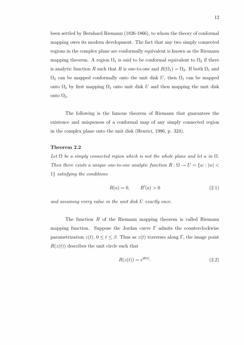
parametrization z(t), 0 ≤ t ≤ β. Thus as z(t) traverses along Γ, the image point
R(z(t)) describes the unit circle such that
R(z(t)) = eiθ(t). (2.2)
13
1
)(t
R(z(t))z(t)
R
Figure 2.3: Boundary correspondence function θ(t).
The argument of R(z(t)) which is θ(t) is known as the boundary
correspondence function for the map R (See Figure 2.3).
2.4 Conformal Mapping of Multiply Connected Regions
A connected region which is not simply connected is called multiply
connected. Such region has holes in it. A region with one hole is called doubly
connected. A region with two holes is called triply connected and so on.
By the Riemann mapping theorem, all the simply connected regions with
more than one boundary point are conformally equivalent to each other. If we
try to introduce the concept of the standard region or canonical domain into
the theory of conformal mapping of multiply connected regions, we meet two
initial obstacles. The first and less serious is the fact that conformal mapping is
continuous and thus preserves the order of connectivity of a region. For example,
a conformal map of a doubly connected region is again a doubly connected region.
Therefore it becomes necessary to introduce distinct canonical regions for each
order of connectivity. The second difficulty is caused by the fact that no exact
equivalent of the Riemann mapping theorem holds in the multiply connected
case. It is not true that any two regions of the some order of connectivity
are conformally equivalent to each other. Not all regions of the same order of
connectivity are of the same conformal type.

14
Let Ω denote a multiply connected region of connectivity M + 1, M =
0, 1, 2, ... such that a Jordan contour Γ0 contains M Jordan contours Γj, j =
1, 2, 3, ..., M , in its interior and the origin is an interior point of Γ1 (see Figure
2.4). The connectivity is taken as M + 1 simply because the value of M tells the
number of holes inside Γ0. The boundary of the multiply connected regions shall
be denoted by Γ = Γ0 ∪ Γ1 ∪ · · · ∪ ΓM .
M
0
21
Figure 2.4: An (M + 1) connected region.
The theorems related to the mapping of multiply connected region are
generally stated in the following form (Kythe, 1998, p. 360; Henrici, 1986, p.
451):
Theorem 2.3
Let Ω be a multiply connected region of connectivity (M + 1) inside the annulus
r < |z| < 1 where Γ0 = |z| = 1 and Γ1 = |z| = r are the two boundary components
of Ω. Then there exists a unique univalent analytic function w = f(z) in Ω such
that (i) it maps Ω conformally onto a region G in the w-plane formed by removing
n concentric circular arcs centered at w = 0 from the annulus ρ < |w| < 1, where
0 < ρ < 1, and (ii) it maps the unit circle Γ0 conformally onto the unit circle
|w| = 1, and the circle |w| < ρ, with f(1) = 1.
Theorem 2.4
Under the hypotheses there exist M real numbers µj, j = 1, 2, 3, ..., M , such that
0 < µM < µj < 1, j = 1, 2, ...,M−1, such that there is an analytic function f that

15
maps Ω conformally onto the annulus µM < |w| < 1, cut along M − 1 mutually
disjoint slits Λj located on the circles |w| = µj, j = 1, 2, ..., M − 1. The mapping
function f can be extended analytically to the curves Γj bounding Ω. The images
of Γ0 and of ΓM are the circles Λ0 : |w| = 1 and ΛM : |w| = Γj respectively. The
image of the curves Γj are the slits Λj, j = 1, 2, ...,M − 1, traversed twice. The
function f is determined up to a factor of modulus 1.
The notations used and the assertions of Theorems 2.3 and 2.4 are
illustrated in Figure 2.5 for the case M = 3.
0
2
1
3
0
1
1
32
Figure 2.5: Mapping of a region of connectivity 4 onto an annulus with circular
slits.
Theorem 2.5
Let Ω be a multiply connected region of connectivity (M + 1) inside the unit disk
|z| < 1 where Γ = |z| = 1 is boundary component of Ω and 0 ∈ Ω. There exists
a unique, univalent analytic function w = f(z) in Ω such that (i) it maps Ω
conformally onto a region G inside the unit disk |w| < 1 which has M circular
cuts centered at w = 0 and (ii) it maps the unit circle |z| = 1 conformally onto
unit circle |w| = 1 with f(0) = 0 and f(1) = 1.
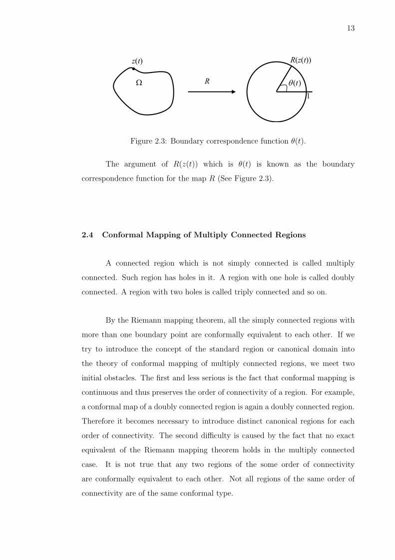
The assertions of Theorem 2.5 is illustrated in Figure 2.6 for the case
M = 3.
16
3
2
0
1
1
2
0
31
Figure 2.6: Mapping of a region of connectivity 4 onto a disk with circular slits.
The boundary correspondence function, θ(t) set up for the simply
connected case can also be extended to the doubly connected regions. Let the
outer and inner boundary curves of a doubly connected region Ω be given in
parametric representation as follows (Henrici, 1986, p. 461) :
Γ0 : z = z0(t), 0 ≤ t ≤ β0,
Γ1 : z = z1(t), 0 ≤ t ≤ β1.
If f is a function which maps the region Ω bounded by Γ0 and Γ1 onto the
annulus A : µ < |w| < 1 so that the inner and the outer boundaries correspond
to each other, the boundary correspondence function θ0 (outer boundary) and θ1
(inner boundary) are continuous function satisfying
f(z0(t)) = eiθ0(t), 0 ≤ t ≤ β0, (2.3)
f(z1(t)) = µeiθ1(t), 0 ≤ t ≤ β1, (2.4)
where the expressions on the left are to be understood as the continuous
extensions of the mapping function to the boundary.

17
2.5 Exact Mapping Function of Doubly Connected Regions for Some
Selected Regions
In this section, we present some of the exact conformal mapping f(z)
of doubly connected regions onto an annulus A = z : r < |w1| < 1, where
0 < r < 1. Later, the exact conformal mapping of annulus onto a unit disk with
a circular slit, denoted by h(z) is given. The composite g = h f then directly
maps the doubly connected regions onto a disk with a circular slit (see Figure
2.7). The special regions considered are annulus, frame of limacon, circular frame,
elliptic frame and frame of Cassini’s oval.
fhg
r~ 1 µ 1
f h
Figure 2.7: The composite g = h f .
2.5.1 Annulus Onto A Disk With A Circular Slit
The exact conformal mapping of doubly connected regions onto a unit
disk with a slit is adapted from von Koppenfels and Stallmann, (1959, p 362).
Consider a frame of circular annulus A = z : r < |z| < 1, r > 0,
Γ0 : z(t) = cos t + i sin t,
Γ1 : z(t) = r(cos t + i sin t), 0 ≤ t ≤ 2π.
Under the mapping p(z) =1
2πlog z, the annulus A is mapped onto the rectangle
R =
w1 = x + i y : 0 < x < π, 0 < y <πτ
2
. (2.5)
18
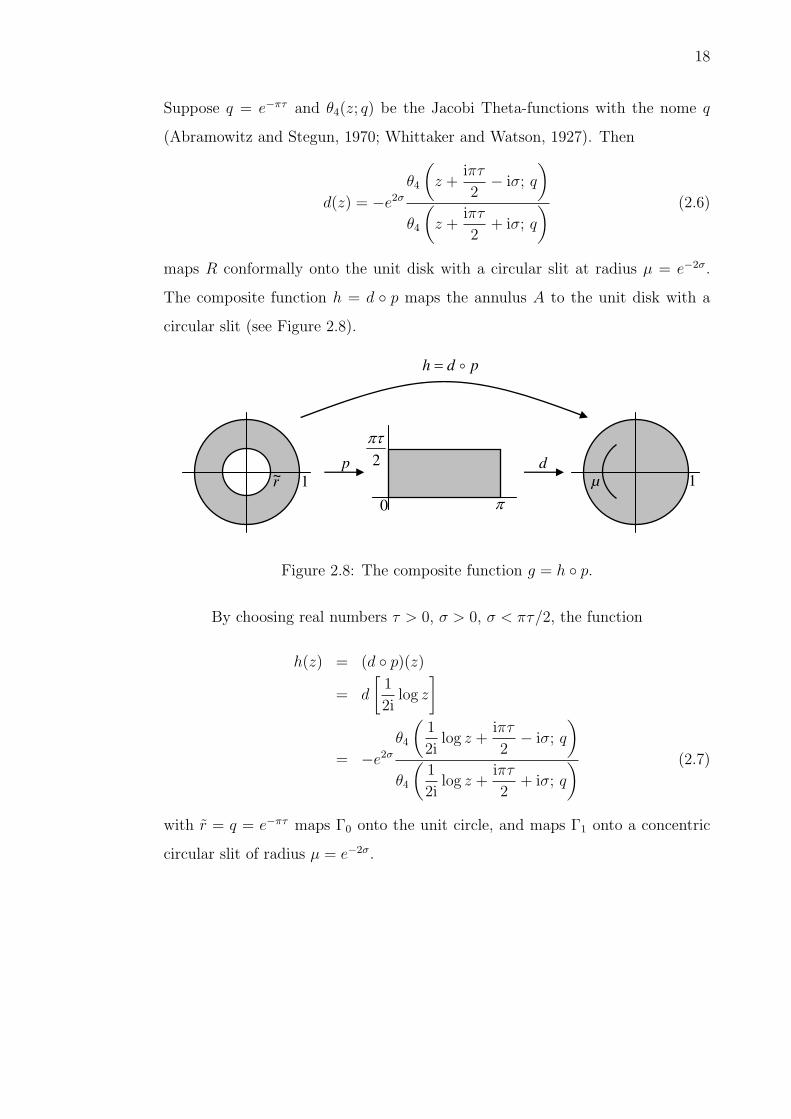
Suppose q = e−πτ and θ4(z; q) be the Jacobi Theta-functions with the nome q
(Abramowitz and Stegun, 1970; Whittaker and Watson, 1927). Then
d(z) = −e2σ
θ4
(z +
iπτ
2− iσ; q
)
θ4
(z +
iπτ
2+ iσ; q
) (2.6)
maps R conformally onto the unit disk with a circular slit at radius µ = e−2σ.
The composite function h = d p maps the annulus A to the unit disk with a
circular slit (see Figure 2.8).
pdh
r~ 1 µ 1
p 2
0
d
Figure 2.8: The composite function g = h p.
By choosing real numbers τ > 0, σ > 0, σ < πτ/2, the function
h(z) = (d p)(z)
= d
[1
2ilog z
]
= −e2σ
θ4
(1
2ilog z +
iπτ
2− iσ; q
)
θ4
(1
2ilog z +
iπτ
2+ iσ; q
) (2.7)
with r = q = e−πτ maps Γ0 onto the unit circle, and maps Γ1 onto a concentric
circular slit of radius µ = e−2σ.

19
2.5.2 Circular Frame
Consider a pair of circles (see Saff and Snider, 2003, A-21)
Γ0 : z(t) = eit,
Γ1 : z(t) = c + ρeit, 0 ≤ t ≤ 2π
such that the domain bounded by Γ0 and Γ1 is the domain between a unit circle
and a circle center at c with radius ρ.
The mapping function given by
f(z) =z − λ
λz − 1(2.8)
with
λ =2c
1 + (c2 − ρ2) +√
(1− (c− ρ)2)(1− (c + ρ)2),
maps Γ0 onto the unit circle and Γ1 onto a circle of radius
r =2ρ
1− (c2 − ρ2) +√
(1− (c− ρ)2)(1− (c + ρ)2).
From Section 2.5.1, we set r = q = e−πτ . This implies τ =ln(r)
−π. We
choose a real number σ such that 0 < σ < πτ/2. Then the mapping function
given by
g(z) = e2σ
θ4
(1
2ilog f(z) +
iπτ
2− iσ; q
)
θ4
(1
2ilog f(z) +
iπτ
2+ iσ; q
) , 0 < σ <πτ
2, (2.9)
maps Γ0 onto the unit circle and Γ1 onto a concentric circular slit of radius
µ = e−2σ.

20
2.5.3 Frame of Limacon
Consider a pair of Limacon (see Kythe, 1998, p. 307)
Γ0 : z(t) = a0 cos t + b0 cos 2t + i(a0 sin t + b0 sin 2t), a0 > 0, b0 > 0,
Γ1 : z(t) = a1 cos t + b1 cos 2t + i(a1 sin t + b1 sin 2t), a1 > 0, b1 > 0,
where t : 0 ≤ t ≤ 2π. When b1/b0 = (a1/a0)2, the mapping function given by
f(z) =
√a2
0 + 4b0z − a0
2b0
, (2.10)
maps Γ0 onto the unit circle and Γ1 onto a circle of radius r =a1
a0
.
We set r = q = e−πτ , this implies τ =ln(r)
−π. We choose a real number σ
satisfying 0 < σ < πτ/2. The mapping function given by
g(z) = −e2σ
θ4
(1
2ilog f(z) +
iπτ
2− iσ; q
)
θ4
(1
2ilog f(z) +
iπτ
2+ iσ; q
) , 0 < σ <πτ
2, (2.11)
then maps Γ0 onto the unit circle and Γ1 onto a concentric circular slit of radius
µ = e−2σ.
2.5.4 Elliptic Frame
Elliptic frame is the domain bounded by two Jordan curves, Γ0 and Γ1
such that
Ω :x2
a20
+y2
b20
< 1,x2
a21
+y2
b21
> 1,
with the complex parametric of its boundary is given by (see Amano, 1994)
Γ0 : z(t) = a0 cos t + ib0 sin t, a0 > 0, b0 > 0,
Γ1 : z(t) = a1 cos t + ib1 sin t, a1 > 0, b1 > 0, 0 ≤ t ≤ 2π.

21
When the two ellipses Γ0 and Γ1 are confocal such that a20 − b2
0 = a21 − b2
1,
the mapping given by
f(z) =z +
√z2 − (a2
0 − b20)
a0 + b0
, r =a1 + b1
a0 + b0
, (2.12)
maps Γ0 onto the unit circle and Γ1 onto a circle of radius r.
We set r = q = e−πτ , this implies τ =ln(r)
−π. We choose a real number σ
satisfying 0 < σ < πτ/2. Then the mapping function given by equation (2.11),
maps Γ0 onto the unit circle and Γ1 onto a concentric circular slit of radius
µ = e−2σ.
2.5.5 Frame of Cassini’s Oval
If Ω is the region bounded by two Cassini’s oval, then the complex
parametric equation of its boundary is given by (see Amano, 1994)
Γ0 : z(t) =
√b20 cos 2t +
√a4
0 − b40 sin2 2t eit, a0 > 0, b0 > 0,
Γ1 : z(t) =
√b21 cos 2t +
√a4
1 − b41 sin2 2t eit, a1 > 0, b1 > 0, 0 ≤ t ≤ 2π,
such that
Ω : |z2 − b20| < a2
0, |z2 − b21| > a2
1.
The boundaries Γ0 and Γ1 are chosen such that (a40−b4
0)/b20 = (a4
1−b41)/b
21.
The mapping given by
f(z) =a0z√
b20z
2 + a40 − b4
0
, r =a0b1
a1b0
, (2.13)
then maps Γ0 onto the unit circle and Γ1 onto a circle of radius r.
We set r = q = e−πτ , this implies τ = − ln(r)/π. We choose a real number
σ satisfying 0 < σ < πτ/2. Then the mapping function given by equation (2.11),
maps Γ0 onto the unit circle and Γ1 onto a concentric circular slit of radius
µ = e−2σ.

22
2.6 Some Numerical Methods for Conformal Mapping of Multiply
Connected Regions
While conformal maps are indispensable tools in many problems of modern
technology, the practical use of conformal maps has always been limited by the
fact that exact conformal maps are only known for certain special regions. Since
conformal maps cannot be obtained in closed form, in general, we have to resort
to numerical approximations of such maps. With the aid of digital computers
which are getting faster and less costly nowadays, much research has been done
to discuss algorithms for the constructions of conformal maps.
Several methods have been proposed in the literature for the numerical
evaluation for conformal mapping of multiply connected regions. For some
perspectives, see Amano (1994), Crowdy and Marshall (2006), Ellacott (1979),
Henrici (1974), Hough and Papmichael (1983), Kokkinos et al. (1990), Mayo
(1986), Murid and Razali (1999), Nasser (2009), Papamicheal and Warby (1984),
Papamicheal and Kokkinos (1984), Okano et al. (2003), Reichel (1986), and
Symm (1969). Generally, these methods fall into three types, namely expansion
method, iterative method, and integral equation method. It is hard to find
methods that are at once fast, accurate, and reliable for conformal mapping
of the multiply connected case because it also involved the unknown conformal
modulus, µ−1 that has to be determined in the course of numerical solution.
The integral equation and iterative methods are more preferable and effective for
numerical conformal mapping.
The classical integral equation method of Symm (1969) is well-known for
computing the conformal maps of doubly connected regions by means of the
singular Fredholm integral equations of the first kind. Some Fredholm integral
equations of the second kind for conformal mapping of doubly connected regions
are of Warschawski and Gerschgorin as discussed in e.g., Henrici (1986). All
these integral equations are extensions of those maps for simply connected regions.

23
However, there are two recently derived integral equations for conformal mapping
of simply connected regions which have no analogue for the doubly connected case.
These are the KST integral equation and the integral equation for the Bergman
kernel as derived in Kerzman and Trummer (1986), Henrici (1986) and Razali
et al. (1997). An effort for such extension has been given by Murid and Razali
(1999). These integral equations are based on a boundary relationship satisfied
by a function which is analytic in a doubly connected region. Next, we present
some well-known numerical methods that have been proposed in the literature
and regarded with great favor for solving numerical conformal mapping of doubly
and multiply connected regions.
2.6.1 Wegmann’s Iterative Method
An iterative method by Wegmann (2005) consider the conformal mapping
from an annulus, A = w : µ < |w| < 1 onto a given doubly connected
region. The method is based on a certain Riemann-Hilbert problem. In view of
its quadratic convergence and its O(n log n) operations count per iteration step,
Wegmann’s method is almost certainly the fastest yet devised for this problem
(see, e.g., Trefethen (1986)).
The conformal mapping Φ : Aµ → Ø, the inverse of the mapping f ,
is uniquely determined up to a rotation of Aµ. To fix this ambiguity one can
impose the condition
Φ(1) = η1(0).
Conjugation on the annulus Aµ is effected by a (real) linear operator Kµ(φ1, φ2)
which is most easily defined in terms of the complex or real Fourier series
φj(t) =∞∑
n=−∞An,j eint = a0,j +
∞∑n=1
(an,j cos nt + bn,j sin nt)

24
of the function φj, j = 1, 2. Then
Kµ(φ1, φ2)(t) =∞∑
n=−∞Bn eint =
∞∑n=1
(αn,j cos nt + βn,j sin nt)
with the coefficients
B0 = 0, Bn :=2iAn,2 − (µ−n − µn)iAn,1
µ−n − µnfor n 6= 0
and
αn :=2bn,2 − (µ−n − µn)bn,1
µ−n − µn, βn :=
2an,2 − (µ−n − µn)an,1
µ−n − µn
for l = 1, 2, .... The analytic solution Φ can be constructed in terms of the
conjugation operator
Φ(eit) = φ1(t) + iKµ(φ1, φ2)(t) + iγ,
Φ(µeit) = φ2(t)− iKµ(φ2, φ1)(t) + iγ,
where γ is an arbitrary real constant.
2.6.2 Symm’s Integral Equations
Symm’s integral equation is one of the well-known integral equation
underlying numerical method for conformal mapping which lies on the potential
theoretic formulation.
The pair of integral equations of first kind which still contain the unknown
parameter µ∫
Γ
log |z − ζ|σ(ζ)|dζ| = − log |z|, z ∈ Γ0,∫
Γ
log |z − ζ|σ(ζ)|dζ| − log µ = − log |z|, z ∈ Γ1,
and the condition equation ∫
Γ1
σ(ζ)|dζ| = 0
are coupled integral equations for densities σ(ζ) and µ and known as Symm’s
integral equations for conformal mapping of doubly connected regions (Symm,
1969).
25
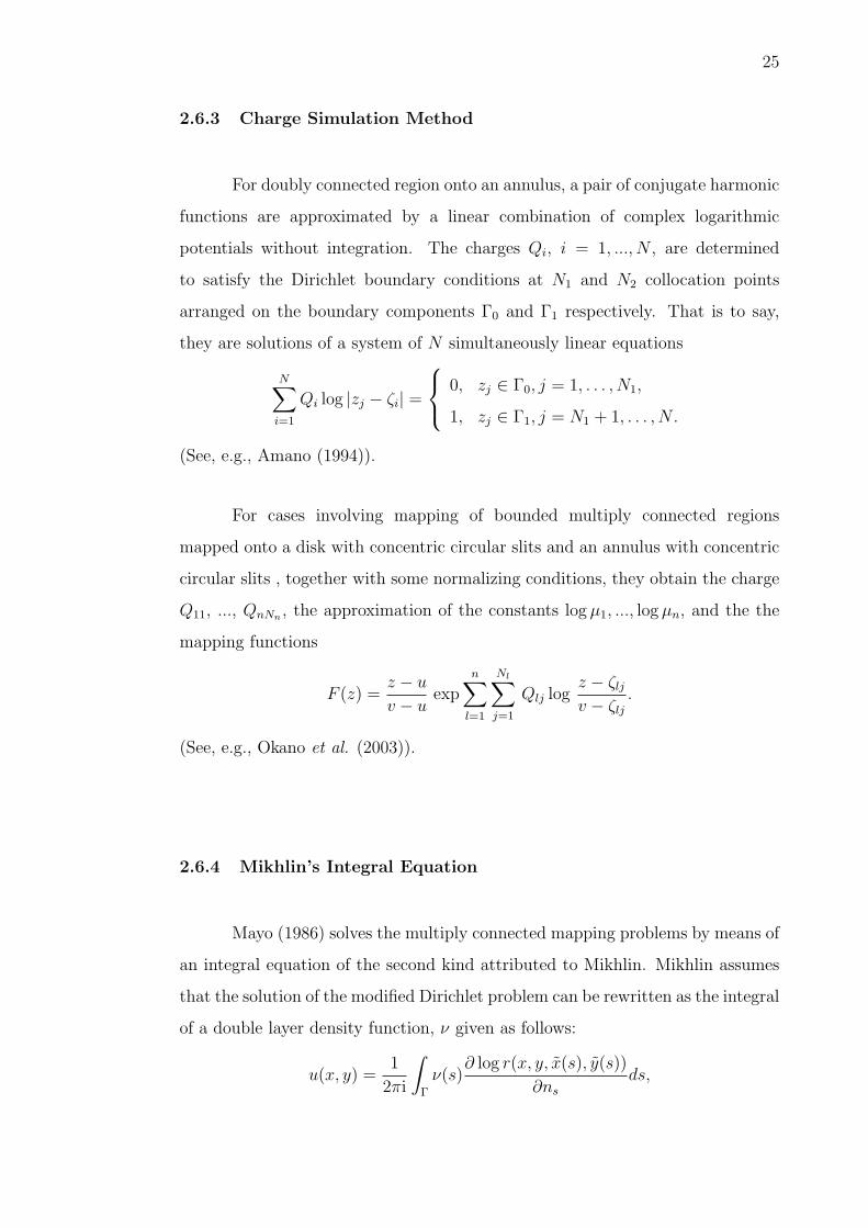
2.6.3 Charge Simulation Method
For doubly connected region onto an annulus, a pair of conjugate harmonic
functions are approximated by a linear combination of complex logarithmic
potentials without integration. The charges Qi, i = 1, ..., N , are determined
to satisfy the Dirichlet boundary conditions at N1 and N2 collocation points
arranged on the boundary components Γ0 and Γ1 respectively. That is to say,
they are solutions of a system of N simultaneously linear equations
N∑i=1
Qi log |zj − ζi| =
0, zj ∈ Γ0, j = 1, . . . , N1,
1, zj ∈ Γ1, j = N1 + 1, . . . , N.
(See, e.g., Amano (1994)).
For cases involving mapping of bounded multiply connected regions
mapped onto a disk with concentric circular slits and an annulus with concentric
circular slits , together with some normalizing conditions, they obtain the charge
Q11, ..., QnNn , the approximation of the constants log µ1, ..., log µn, and the the
mapping functions
F (z) =z − u
v − uexp
n∑
l=1
Nl∑j=1
Qlj logz − ζlj
v − ζlj
.
(See, e.g., Okano et al. (2003)).
2.6.4 Mikhlin’s Integral Equation
Mayo (1986) solves the multiply connected mapping problems by means of
an integral equation of the second kind attributed to Mikhlin. Mikhlin assumes
that the solution of the modified Dirichlet problem can be rewritten as the integral
of a double layer density function, ν given as follows:
u(x, y) =1
2πi
∫
Γ
ν(s)∂ log r(x, y, x(s), y(s))
∂ns
ds,

26
where
r2 = (x− x(s))2 + (y − y(s))2.
Mikhlin showed that the solution ν(t) can be determined from the integral
equation
ν(t) +1
π
∫
Γ
ν(s)
[∂ log r(s, t)
∂ns
− a(s, t)
]ds = −2 log |t− α|,
where
a(s, t) =
1, if s, t lie on the same curve,
0, otherwise.
2.6.5 Fredholm Integral Equation
Reichel (1986) describes a fast iterative method for solving Fredholm
integral equations of the first kind whose kernels have a logarithmic principal part
for multiply connected regions. The method is a Fourier-Galerkin method, and
due to the singularity of the kernel, the linear system of simultaneous equations
is block diagonally dominant and can be solved rapidly by an iterative method.
The numerical method involves solving the the system of integral equations
qk +n∑
j=1
∫
Γj
ln1
|z − ζ|σj(ζ)|dζ| = fk(z), z ∈ Γk, 1 ≤ k ≤ n,
∫
Γk
σk(ζ)|dζ| = 0, 1 ≤ k ≤ n.
for qj ∈ R, σ∗j ∈ L2(Γj). The mapping function φ(z) is defined by
φ(z) := z exp
(n∑
j=1
∫
Γj
ln1
(z − ζ)σ∗j (ζ)|dζ|
).

27
2.6.6 Warschawski’s and Gershgorin’s Integral Equations
Henrici (1986) discussed two classical integral equations underlying
numerical conformal mapping for doubly connected regions which are
Warschawski’s and Gershgorin’s integral equations. These well-known integral
equations are stated in Theorem 2.6 and 2.7 (see, Henrici, 1986, p. 466-468).
Theorem 2.6 (Warschawski’s Integral Equations for Doubly Connected Regions)
If the boundary curves are such that z′′i is continuous and the boundary
correspondence functions θ′i have continuous derivatives, then the function θ′0 and
θ′1 satisfy the system of integral equations
θ′0(σ) +
∫ β0
0
v0,0(τ, σ)θ′0(τ) dτ −∫ β1
0
v0,1(τ, σ)θ′1(τ) dτ = 0,
θ′1(σ) +
∫ β0
0
v1,0(τ, σ)θ′0(τ) dτ −∫ β1
0
v1,1(τ, σ)θ′1(τ) dτ = 0,
where the kernels vi,j are the Neumann kernels defined as
v0,0(τ, σ) =1
πIm
z′0(σ)
z0(σ)− z0(τ),
v0,1(τ, σ) =1
πIm
z′0(σ)
z0(σ)− z1(τ),
v1,0(τ, σ) =1
πIm
z′1(σ)
z1(σ)− z0(τ),
v1,1(τ, σ) =1
πIm
z′1(σ)
z1(σ)− z1(τ).
Theorem 2.7 (Gershgorin’s Integral Equations for Doubly Connected Regions)
Under the hypothesis of Theorem 2.6, the functions θ′0 and θ′1 satisfy the system
of integral equations
θ0(σ)−∫ β0
0
v0,0(σ, τ)θ0(τ) dτ +
∫ β1
0
v1,0(σ, τ)θ1(τ) dτ = 2 argz0(σ)− z1(0)
z0(σ)− z0(0),
θ1(σ)−∫ β0
0
v0,1(σ, τ)θ0(τ) dτ +
∫ β1
0
v1,1(σ, τ)θ1(τ) dτ = 2 argz1(σ)− z1(0)
z1(σ)− z0(0).
Both, the Warschawski’s and Gershgorin’s integral equations do not
involve the modulus µ−1 of the given doubly connected regions. If the functions

28
θ0, θ1 and/or their derivatives are known, the modulus may be determined from
the following formula:
Log1
µ= log
∣∣∣∣z0(0)− z
z1(0)− z
∣∣∣∣−1
2π
∫ β0
0
Rez′0(τ)
z0(τ)− zθ0(τ) dτ
+1
2π
∫ β1
0
Rez′1(τ)
z1(τ)− zθ1(τ) dτ, (2.14)
which holds for arbitrary z interior to Γ1.
2.6.7 The Boundary Integral Equation via the Kerzman-Stein and
the Neumann Kernels
Based on a certain boundary relationship satisfied by a function which
is analytic in a region interior to a closed Jordan curve, Murid et al. (1999)
construct a boundary integral equation related to the analytic function. Special
realizations of this integral equation are the integral equations related to the
Szego kernel, the Bergman kernel, and the Riemann map. The kernels arise in
the integral equations are the Kerzman-Stein kernel and the Neumann kernel.
Murid and Razali (1999) extend the similar construction to a doubly
connected region using a boundary relationship
D(z) = c(z)
[T (z)Q(z)D(z)
P (z)
]−, z ∈ Γ, (2.15)
where D(z) is analytic and single-valued with respect to z ∈ Ω and is continuous
on Ω ∪ Γ, while c, P, and Q are complex-valued functions defined on Γ with the
following properties:
(P1) c(z) =
c0, z ∈ Γ0,
c1, z ∈ Γ1,
(P2) P (z) is analytic and single-valued with respect to z ∈ Ω,

29
(P3) P (z) is continuous on Ω ∪ Γ,
(P4) P (z) has a finite number of zeroes at a1, a2, . . . , an,
(P5) P (z) 6= 0, Q(z) 6= 0, z ∈ Γ.
The integral equation for D that is related to the boundary relationship (2.15) is
as shown below (Murid and Razali, 1999).
Theorem 2.8
Let u and v be any complex-valued functions that are defined on Γ. Then
1
2
[v(z) +
u(z)
T (z)Q(z)
]D(z)
+ PV1
2πi
∫
Γ
[u(z)
(w − z)Q(w)− v(z)T (w)
w − z
]D(w) |dw|
= −c(z)u(z)
∑
ajinsideΓ
Resw=aj
D(w)
(w − z)P (w)
−
− u(z)(c0 − c1)
[1
2πi
∫
Γ2
D(w)
(w − z)P (w)dw
]−, z ∈ Γ, (2.16)
where the minus sign in the superscript denotes complex conjugation and where
Γ2 =
−Γ1, if z ∈ Γ0,
Γ0, if z ∈ Γ1.
Special realization of this integral equation with the assignment
c(z) = i|f(z)|, P (z) = f(z), D(z) =√
f ′(z), Q(z) = 1, (2.17)
and the choice of u(z) = T (z)Q(z) and v(z) = 1 is the integral equation with the
Kerzman-Stein kernel, i.e.,
√f ′(z) +
∫
Γ
A(z, w)√
f ′(w)|dw|
= −i(1− µ)T (z)
[1
2πi
∫
Γ2
√f ′(w)
(w − z)f(w)dw
]−, z ∈ Γ, (2.18)

30
where
A(z, w) =
H(w, z)−H(z, w), if w, z ∈ Γ, w 6= z,
0, if w = z ∈ Γ,
and
H(w, z) =1
2πi
T (z)
(z − w), w ∈ Ω ∪ Γ, z ∈ Γ, w 6= z.
The kernel A is known as the Kerzman-Stein kernel (Kerzman and Trummer,
1986) and is smooth and skew-Hermitian. The kernel H is usually referred to as
the Cauchy kernel.
Another realization of the boundary integral equation with the assignment
c(z) = −|f(z)|2, P (z) = f(z)2, D(z) = f ′(z), Q(z) = T (z), (2.19)
and the choice of u(z) = T (z)Q(z) and v(z) = 1 is given as
f ′(z)+
∫
Γ
M(z, w)f ′(w)|dw| = (1−µ2)T (z)2
[1
2πi
∫
Γ2
f ′(w)
(w − z)f(w)dw
]−, z ∈ Γ,
(2.20)
where
M(z, w) =
T (w)
2πi
[T (z)
2
w − z− 1
w − z
], if w, z ∈ Γ, w 6= z,
1
2π
Im[z′′(t)z′(t)]|z′(t)|3 , if w = z ∈ Γ.
Multiplying both sides of (2.20) by T (z) and using the fact that
T (z)T (z) = |T (z)|2 = 1 gives
T (z)f ′(z) +
∫
Γ
N(z, w)T (w)f ′(w)|dw|
= (1− µ2)T (z)
[1
2πi
∫
Γ2
f ′(w)
(w − z)f(w)2dw
]−, z ∈ Γ, (2.21)
where N is the Neumann kernel (see, e.g., Henrici, 1986, p. 282) defined by
N(z, w) =
1
πIm
[T (z)
z − w
], if w, z ∈ Γ, w 6= z,
1
2π
Im[z′′(t)z′(t)]|z′(t)|3 , if w = z ∈ Γ.
(2.22)

31
However, the integral equations (2.18) and (2.21) are not in the form of
Fredholm integral equations and no numerical experiments have been reported in
Murid and Razali (1999). In Chapter 3, we shows the integral equations (2.18)
can be modified to a numerically tractable integral equation which involves the
unknown inner radius, µ.
In this project, we also derive some boundary integral equation satisfied by
a function analytic on a multiply connected regions subject to certain conditions.
This derivation improves the boundary integral equation (2.16) derived by Murid
and Razali (1999) which was limited to doubly connected regions. Furthermore
it leads to a much simpler derivation of a system of an integral equations
developed in Chapter 3. Another two special cases of this result are the integral
equation involving the Neumann kernel related to conformal mapping of multiply
connected regions onto an annulus with circular slits and onto a disk with circular
slits. All these are described in Chapter 4 and the numerical conformal mappings
are discussed in Chapters 5 and 6.

CHAPTER 3
AN INTEGRAL EQUATION METHOD FOR CONFORMAL
MAPPING OF DOUBLY CONNECTED REGIONS VIA THE
KERZMAN-STEIN KERNEL
3.1 Introduction
Let the outer and inner boundary curves be given in parametric
representation as follows:
Γ0 : z = z0(t), 0 ≤ t ≤ β0,
Γ1 : z = z1(t), 0 ≤ t ≤ β1.
If f is a function which maps the region Ω bounded by Γ0 and Γ1
onto the annulus A = w : µ < |w| < 1 so that the inner and the outer
boundaries correspond to each other, the boundary correspondence function θ0
(outer boundary) and θ1 (inner boundary) are continuous functions satisfying
f(z0(t)) = eiθ0(t), 0 ≤ t ≤ β0, (3.1)
f(z1(t)) = µeiθ1(t), 0 ≤ t ≤ β1. (3.2)
33
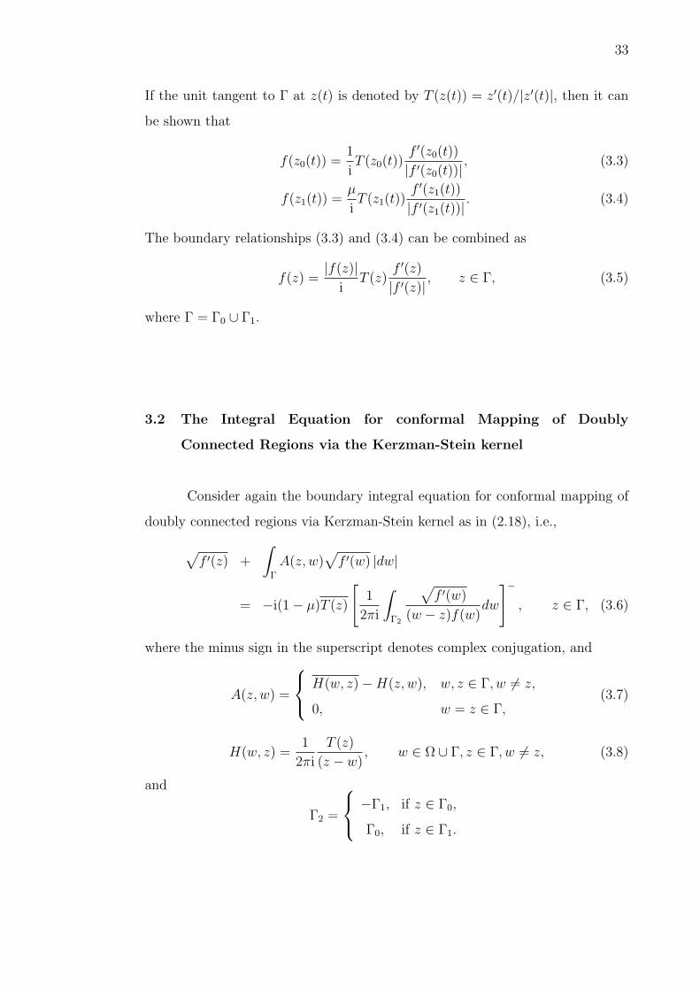
If the unit tangent to Γ at z(t) is denoted by T (z(t)) = z′(t)/|z′(t)|, then it can
be shown that
f(z0(t)) =1
iT (z0(t))
f ′(z0(t))
|f ′(z0(t))| , (3.3)
f(z1(t)) =µ
iT (z1(t))
f ′(z1(t))
|f ′(z1(t))| . (3.4)
The boundary relationships (3.3) and (3.4) can be combined as
f(z) =|f(z)|
iT (z)
f ′(z)
|f ′(z)| , z ∈ Γ, (3.5)
where Γ = Γ0 ∪ Γ1.
3.2 The Integral Equation for conformal Mapping of Doubly
Connected Regions via the Kerzman-Stein kernel
Consider again the boundary integral equation for conformal mapping of
doubly connected regions via Kerzman-Stein kernel as in (2.18), i.e.,
√f ′(z) +
∫
Γ
A(z, w)√
f ′(w) |dw|
= −i(1− µ)T (z)
[1
2πi
∫
Γ2
√f ′(w)
(w − z)f(w)dw
]−, z ∈ Γ, (3.6)
where the minus sign in the superscript denotes complex conjugation, and
A(z, w) =
H(w, z)−H(z, w), w, z ∈ Γ, w 6= z,
0, w = z ∈ Γ,(3.7)
H(w, z) =1
2πi
T (z)
(z − w), w ∈ Ω ∪ Γ, z ∈ Γ, w 6= z, (3.8)
and
Γ2 =
−Γ1, if z ∈ Γ0,
Γ0, if z ∈ Γ1.

34
The single integral equation in (3.6) can be separated into a system of two
integral equations given by
√f ′(z0) +
∫
Γ
A(z0, w)√
f ′(w) |dw|
= − i(1−µ)T (z0)
[1
2πi
∫
−Γ1
√f ′(w)
(w − z0)f(w)dw
]−, z = z0 ∈ Γ0,(3.9)
√f ′(z1) +
∫
Γ
A(z1, w)√
f ′(w) |dw|
= − i(1−µ)T (z1)
[1
2πi
∫
Γ0
√f ′(w)
(w − z1)f(w)dw
]−, z = z1 ∈ Γ1.(3.10)
Taking the boundary relationship (3.5) into account, (3.9) and (3.10)
become
√f ′(z0) +
∫
Γ
A(z0, w)√
f ′(w) |dw|
= −i(1−µ)T (z0)
1
2πi
∫
−Γ1
√f ′(w)
(w − z0)[
µiT (w) f ′(w)
|f ′(w)|
]dw
−
, z = z0 ∈ Γ0,
(3.11)√
f ′(z1) +
∫
Γ
A(z1, w)√
f ′(w) |dw|
= −i(1−µ)T (z1)
1
2πi
∫
Γ0
√f ′(w)
(w − z1)[
1iT (w) f ′(w)
|f ′(w)|
]dw
−
, z = z1 ∈ Γ1.
(3.12)
Using |f ′(w)| =√
f ′(w)√
f ′(w) and T (w) |dw| = dw, after some
mathematical manipulations, integral equations (3.11) and (3.12) become
√f ′(z0) +
∫
Γ
A(z0, w)√
f ′(w) |dw|
=1
2πiµ(1−µ)T (z0)
∫
−Γ1
√f ′(w)
(w − z0)|dw|, z = z0 ∈ Γ0, (3.13)
√f ′(z1) +
∫
Γ
A(z1, w)√
f ′(w) |dw|
=1
2πi(1−µ)T (z1)
∫
Γ0
√f ′(w)
(w − z1)|dw|, z = z1 ∈ Γ1. (3.14)

35
Since Γ = Γ0 ∪ Γ1 , (3.13) and (3.14) may be written as
√f ′(z0)+
∫
Γ0
A(z0, w)√
f ′(w) |dw|−∫
−Γ1
A(z0, w)√
f ′(w) |dw|
=1
2πiµ
∫
−Γ1
T (z0)
(w − z0)
√f ′(w) |dw| − 1
2πi
∫
−Γ1
T (z0)
(w − z0)
√f ′(w) |dw|, z = z0 ∈ Γ0,
√f ′(z1)+
∫
Γ0
A(z1, w)√
f ′(w) |dw|−∫
−Γ1
A(z1, w)√
f ′(w) |dw|
=1
2πi
∫
Γ0
T (z1)
(w − z1)
√f ′(w) |dw| − µ
2πi
∫
Γ0
T (z1)
(w − z1)
√f ′(w) |dw|, z = z1 ∈ Γ1.
Applying definition (3.7) to A(z0, w) in∫−Γ1
of the first equation, and to A(z1, w)
in∫
Γ0of the second equation, we obtain
√f ′(z0) +
∫
Γ0
A(z0, w)√
f ′(w) |dw| −∫
−Γ1
1
2πi
[T (z0)
(w − z0)− T (w)
(w − z0)
] √f ′(w) |dw|
=1
2πiµ
∫
−Γ1
T (z0)
(w − z0)
√f ′(w) |dw| − 1
2πi
∫
−Γ1
T (z0)
(w − z0)
√f ′(w) |dw|, z = z0 ∈ Γ0,
√f ′(z1) +
∫
Γ0
1
2πi
[T (z1)
(w − z1)− T (w)
(w − z1)
] √f ′(w) |dw| −
∫
−Γ1
A(z1, w)√
f ′(w) |dw|
=1
2πi
∫
Γ0
T (z1)
(w − z1)
√f ′(w) |dw| − µ
2πi
∫
Γ0
T (z1)
(w − z1)
√f ′(w) |dw|, z = z1 ∈ Γ1.
After some cancellations, we get
√f ′(z0) +
∫
Γ0
A(z0, w)√
f ′(w) |dw|+ 1
2πi
∫
−Γ1
T (w)
(w − z0)
√f ′(w) |dw|
=1
2πiµ
∫
−Γ1
T (z0)
(w − z0)
√f ′(w) |dw|, z = z0 ∈ Γ0, (3.15)
√f ′(z1) − 1
2πi
∫
Γ0
T (w)
(w − z1)
√f ′(w) |dw| −
∫
−Γ1
A(z1, w)√
f ′(w) |dw|
= − µ
2πi
∫
Γ0
T (z1)
(w − z1)
√f ′(w) |dw|, z = z1 ∈ Γ1. (3.16)
Rearranging, (3.15) and (3.16) yield
√f ′(z0)+
∫
Γ0
A(z0, w)√
f ′(w) |dw|
−∫
−Γ1
1
2πi
[T (z0)
µ(w − z0)− T (w)
(w − z0)
]√f ′(w) |dw| = 0, z = z0 ∈ Γ0, (3.17)

36
√f ′(z1)+
∫
Γ0
1
2πi
[µT (z1)
(w − z1)− T (w)
(w − z1)
]√f ′(w) |dw|
−∫
−Γ1
A(z1, w)√
f ′(w) |dw| = 0, z = z1 ∈ Γ1. (3.18)
Note that there are three unknown quantities in the integral equations
(3.17) and (3.18), namely,√
f ′(z0) ,√
f ′(z1) and µ. For numerical purposes,
a third equation involving µ is needed so that the system of integral equations
above can be solved simultaneously.
Consider equations (3.1) and (3.2) which on differentiation give
f ′(z0(t))z′0(t) = eiθ0(t)iθ′0(t),
f ′(z1(p))z′1(p) = µeiθ1(p)iθ′1(p).
Taking the modulus on both sides of the equations, we obtain
|f ′(z0(t))z′0(t)| = |eiθ0(t)iθ′0(t)| = |eiθ0(t)|i|θ′0(t)|, (3.19)
|f ′(z1(t))z′1(p)| = |µeiθ1(p)iθ′1(p)| = |µ||eiθ1(p)|i|θ′1(p)|. (3.20)
The absolute values of eiθ0(t) and eiθ1(p) are both equal to 1. The boundary
correspondence functions θ0(t) and θ1(p) are increasing monotone functions and
thus the derivative of them are never negative which imply |θ′0(t)| = θ′0(t) and
|θ′1(p)| = θ′1(p). The quantity µ is the inner radius of the annulus A = w : µ <
|w| < 1 where 0 < µ < 1 . Thus (3.19) and (3.20) can now be written as
|f ′(z0(t))z′0(t)| = θ′0(t), (3.21)
|f ′(z1(t))z′1(p)| = µθ′1(p). (3.22)
Upon integrating (3.21) and (3.22) with respect to t and p respectively from 0 to
2π gives
∫ 2π
0
|f ′(z0(t))z′0(t)| dt =
∫ 2π
0
θ′0(t) dt = θ′0(t)|2π0 = 2π, (3.23)
∫ 2π
0
|f ′(z1(p))z′1(p)| dp = µ
∫ 2π
0
θ′1(p) dp = µθ′1(p)|2π0 = µ2π. (3.24)
37
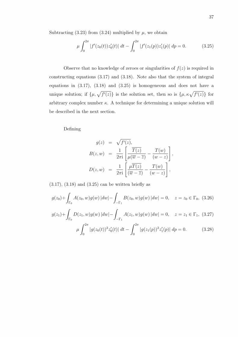
Subtracting (3.23) from (3.24) multiplied by µ, we obtain
µ
∫ 2π
0
|f ′(z0(t))z′0(t)| dt−
∫ 2π
0
|f ′(z1(p))z′1(p)| dp = 0. (3.25)
Observe that no knowledge of zeroes or singularities of f(z) is required in
constructing equations (3.17) and (3.18). Note also that the system of integral
equations in (3.17), (3.18) and (3.25) is homogeneous and does not have a
unique solution; if µ,√
f ′(z) is the solution set, then so is µ, κ√
f ′(z) for
arbitrary complex number κ. A technique for determining a unique solution will
be described in the next section.
Defining
g(z) =√
f ′(z),
B(z, w) =1
2πi
[T (z)
µ(w − z)− T (w)
(w − z)
],
D(z, w) =1
2πi
[µT (z)
(w − z)− T (w)
(w − z)
],
(3.17), (3.18) and (3.25) can be written briefly as
g(z0)+
∫
Γ0
A(z0, w)g(w) |dw|−∫
−Γ1
B(z0, w)g(w) |dw| = 0, z = z0 ∈ Γ0, (3.26)
g(z1)+
∫
Γ0
D(z1, w)g(w) |dw|−∫
−Γ1
A(z1, w)g(w) |dw| = 0, z = z1 ∈ Γ1, (3.27)
µ
∫ 2π
0
|g(z0(t))2z′0(t)| dt−
∫ 2π
0
|g(z1(p))2z′1(p)| dp = 0. (3.28)

38
3.3 Numerical Implementation
Using parametric representation z0(t) of Γ0 for t : 0 ≤ t ≤ β0 and z1(p) of
Γ1 for p : 0 ≤ p ≤ β1, (3.26) and (3.27) become
g(z0(t)) +
∫ β0
0
A(z0(t), z0(s))g(z0(s))|z′0(s)| ds
−∫ β1
0
B(z0(t), z1(q))g(z1(q))|z′1(q)| dq = 0, z0(t) ∈ Γ0, (3.29)
g(z1(p)) +
∫ β0
0
D(z1(p), z0(s))g(z0(s))|z′0(s)| ds
−∫ β1
0
A(z1(p), z1(q))g(z1(q))|z′1(q)| dq = 0, z1(p) ∈ Γ1. (3.30)
Multiply (3.29) and (3.30) respectively by |z′0(t)|1/2 and |z′1(p)|1/2 gives
|z′0(t)|1/2g(z0(t)) +
∫ β0
0
|z′0(t)|1/2|z′0(s)|1/2A(z0(t), z0(s))g(z0(s))|z′0(s)|1/2 ds
−∫ β1
0
|z′0(t)|1/2|z′1(q)|1/2B(z0(t), z1(q))g(z1(q))|z′1(q)|1/2 dq = 0, z0(t) ∈ Γ0,
(3.31)
|z′1(p)|1/2g(z1(p)) +
∫ β0
0
|z′1(p)|1/2|z′0(s)|1/2D(z1(p), z0(s))g(z0(s))|z′0(s)|1/2 ds
−∫ β1
0
|z′1(p)|1/2|z′1(q)|1/2A(z1(p), z1(q))g(z1(q))|z′1(q)|1/2 dq = 0, z1(p) ∈ Γ1.
(3.32)
Defining
φ0(t) = |z′0(t)|1/2g(z0(t)),
φ1(p) = |z′1(p)|1/2g(z1(p)),
K00(t, s) = |z′0(t)|1/2|z′0(s)|1/2A(z0(t), z0(s)),
K01(t, q) = |z′0(t)|1/2|z′1(q)|1/2B(z0((t), z1(q)),
K10(p, s) = |z′1(p)|1/2|z′0(s)|1/2D(z1(p), z0(s)),
K11(p, q) = |z′1(p)|1/2|z′1(q)|1/2A(z1(p), z1(q)),
and so (3.31) and (3.32) become
φ0(t) +
∫ β0
0
K00(t, s) φ0(s) ds−∫ β1
0
K01(t, q) φ1(q) dq = 0, z0(t) ∈ Γ0, (3.33)

39
φ1(p)+
∫ β0
0
K10(p, s) φ0(s) ds−∫ β1
0
K11(p, q) φ1(q) dq = 0, z1(p) ∈ Γ1. (3.34)
Note that the kernel K00(t, s) and K11(p, q) preserve the skew-Hermitian
properties. Applying the same procedure to the third equation (3.28), we get
µ
∫ 2π
0
|φ0(t)| 2 dt−∫ 2π
0
|φ1(p)| 2 dp = 0. (3.35)
which is the third equation involving µ that can be solved simultaneously with
integral equations (3.33) and (3.34).
Choosing n equidistant collocation points ti = (i − 1)β0/n, 1 ≤ i ≤ n
and m equidistant collocation points pı = (ı −1)β1/m , 1 ≤ ı ≤ m and applying
the trapezoidal rule for Nystrom’s method to discretize (3.33), (3.34) and (3.35),
we obtain
φ0(ti) +β0
n
n∑j=1
K00(ti, tj) φ0(tj)− β1
m
m∑=1
K01(ti, p) φ1(p) = 0, (3.36)
φ1(pı) +β0
n
n∑j=1
K10(pı, tj) φ0(tj) − β1
m
m∑=1
K11(pı, p)φ1(p) = 0, (3.37)
µβ0
n
n∑i=1
|φ0(ti)|2 − β1
m
m∑ı=1
|φ1(pı)|2 = 0. (3.38)
Note that in the third equation (3.38),
|φ0| =√
(Re φ0)2 + (Im φ0)2,
|φ1| =√
(Re φ1)2 + (Im φ1)2.
Equations (3.36), (3.37) and (3.38) lead to a system of (n + m + 1) non-
linear complex equations in n unknowns φ0(ti), m unknowns φ1(pı) and µ. By
defining the matrices
Bij =β0
nK00(ti, tj),
Ciı =β1
mK01(ti, p),
Eıj =β0
nK10(pı, tj),
Dıı =β1
mK11(pı, p),
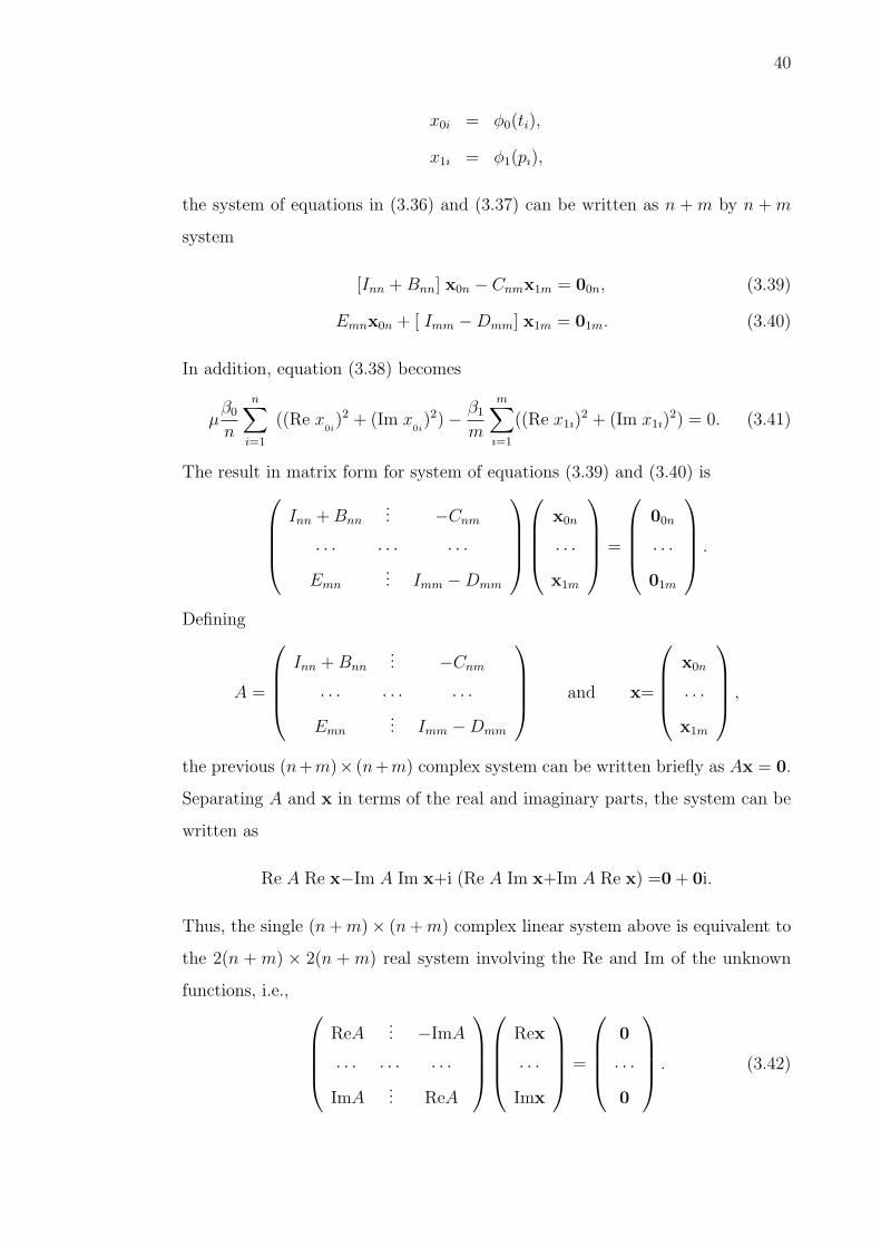
40
x0i = φ0(ti),
x1ı = φ1(pı),
the system of equations in (3.36) and (3.37) can be written as n + m by n + m
system
[Inn + Bnn] x0n − Cnmx1m = 00n, (3.39)
Emnx0n + [ Imm −Dmm] x1m = 01m. (3.40)
In addition, equation (3.38) becomes
µβ0
n
n∑i=1
((Re x0i)2 + (Im x
0i)2)− β1
m
m∑ı=1
((Re x1ı)2 + (Im x1ı)
2) = 0. (3.41)
The result in matrix form for system of equations (3.39) and (3.40) is
Inn + Bnn... −Cnm
· · · · · · · · ·Emn
... Imm −Dmm
x0n
· · ·x1m
=
00n
· · ·01m
.
Defining
A =
Inn + Bnn... −Cnm
· · · · · · · · ·Emn
... Imm −Dmm
and x=
x0n
· · ·x1m
,
the previous (n+m)× (n+m) complex system can be written briefly as Ax = 0.
Separating A and x in terms of the real and imaginary parts, the system can be
written as
Re A Re x−Im A Im x+i (Re A Im x+Im A Re x) =0 + 0i.
Thus, the single (n + m)× (n + m) complex linear system above is equivalent to
the 2(n + m) × 2(n + m) real system involving the Re and Im of the unknown
functions, i.e.,
ReA... −ImA
· · · · · · · · ·ImA
... ReA
Rex
· · ·Imx
=
0
· · ·0
. (3.42)
41
Therefore, the linear system above can be solved simultaneously with the
non-linear equation (3.41) which also involves the Re and Im parts of the unknown
functions. Since the system of integral equations (3.17), (3.18) and (3.25) has no
unique solution, the system of equations (3.42) and (3.41) also in general has no
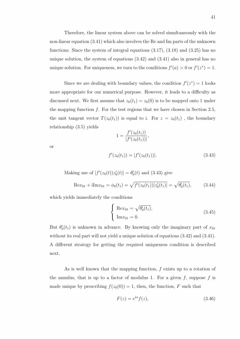
unique solution. For uniqueness, we turn to the conditions f ′(a) > 0 or f ′(z∗) = 1.
Since we are dealing with boundary values, the condition f ′(z∗) = 1 looks
more appropriate for our numerical purpose. However, it leads to a difficulty as
discussed next. We first assume that z0(t1) = z0(0) is to be mapped onto 1 under
the mapping function f . For the test regions that we have chosen in Section 2.5,
the unit tangent vector T (z0(t1)) is equal to i. For z = z0(t1) , the boundary
relationship (3.5) yields
1 =f ′(z0(t1))
|f ′(z0(t1))| ,
or
f ′(z0(t1)) = |f ′(z0(t1))|. (3.43)
Making use of |f ′(z0(t))z′0(t)| = θ′0(t) and (3.43) give
Rex01 + iImx01 = φ0(t1) =√
f ′(z0(t1))|z′0(t1)| =√
θ′0(t1), (3.44)
which yields immediately the conditions
Rex01 =√
θ′0(t1),
Imx01 = 0.(3.45)
But θ′0(t1) is unknown in advance. By knowing only the imaginary part of x01
without its real part will not yield a unique solution of equations (3.42) and (3.41).
A different strategy for getting the required uniqueness condition is described
next.
As is well known that the mapping function, f exists up to a rotation of
the annulus, that is up to a factor of modulus 1. For a given f , suppose f is
made unique by prescribing f(z0(0)) = 1, then, the function, F such that
F (z) = eiαf(z), (3.46)

42
for arbitrary α ∈ <, also maps a doubly connected region onto an annulus.
Differentiating (3.46) gives
F ′(z) = eiαf ′(z) or√
F ′(z) =√
eiαf ′(z). (3.47)
Note that if µ,√
f ′(z) is a solution set of (3.17), and (3.18), then so is
µ, κ√
F ′(z) = µ, κ√
eiαf ′(z) where κ is any complex number, C.
Suppose
F ∗(z) = reiαf(z), r, α ∈ <. (3.48)
is a mapping function that maps a doubly connected region onto an annulus
A∗ = w : rµ < |w| < r. Thus Arg(F ∗(z)). Thus Arg(f(z)) differ by α.
Differentiating (3.48), gives
F ∗′(z) = reiαf ′(z) or√
F ∗′(z) =√
reiαf ′(z). (3.49)
Since√
r ∈ < ⊆ C, then µ,√
F ∗′(z) is also a solution set of our integral
equations (3.17) and (3.18). Note that F ∗′ also satisfies (3.25).
The boundary relationship (3.5) implies
eiαf(z) =|eiαf(z)|
iT (z)
reiαf ′(z)
|reiαf ′(z)| , z ∈ Γ. (3.50)
Since eiαf(z) = F (z) and reiαf(z) = F ∗(z), (3.50) can also be written as
F (z) =|F (z)|
iT (z)
F ∗′(z)
|F ∗′(z)| , z ∈ Γ, (3.51)
where |F (z)| is either 1 or µ. The idea now is to solve for the unique solution√
F ∗′(z) from the system of integral equations (3.17), (3.18) and (3.25) with a
prescribing value of F ∗′(z0(0)). If F ∗′(z0(0)) = B∗, then
φ0(t1) = Re x01 + iIm x01 =√
F ∗′(z0(t1))|z′0(t1)| =√
B∗ |z′0(t1)|.

43
or
Re x01 = Re√
B∗ |z′0(t1)|,Im x01 = Im
√B∗ |z′0(t1)|.
(3.52)
The boundary values of F (z) are then computed according to equation (3.51).
By means of equation (3.46), we then have
f(z) = e−iαF (z), z ∈ Γ.
It remains to determine α. Observe that
F ∗(z0(t)) = reiαf(z0(t)) = reiαeiθ0(t). (3.53)
Differentiating (3.53), we obtain
F ∗′(z0(t))z′0(t) = reiαiθ′0(t)e
iθ0(t).
Substituting t1 = 0, gives
F ∗′(z0(0))z′0(0) = reiαiθ′0(0).
Since F ∗′(z0(0)) = B∗, α is then calculated by the formula
α = Arg[−iz′0(0)B∗]. (3.54)
The system of equations (3.42), (3.41) and (3.52) is an over-determined
system of non-linear equations involving 2(n + m) + 3 equations in 2(n + m) + 1
unknowns. Method for solving system having unequal number of equations and
unknowns are best dealt with as problems in optimization (Woodford, 1992, p.
146). The solution of this system of equations will coincide with the minimizer of
a function which is produced by taking the sum of squares of the left-hand sides
of the over-determined system of the non-linear equations (the right-hand sides
of the equations being zero). We use Gauss-Newton algorithm to solve this non-
linear least square problem which is a modification of Newton’s method. Some
discussion on this method can be found in, see e.g., Antia (1991, pp. 271-345),
Murray (1972, pp. 29-55) and Wolfe (1978, pp. 218-247).

44
Our non-linear least squares problem consists in finding the vector p for
which the function S : R2(n+m)+3 → R1 defined by the sum
S(p) = fT f =
2(n+m)+3∑i=1
(fi(p))2
is minimal. Here, p stands for the (2n+2m+1)-vector (Rex01, Rex02, ..., Rex0n,
Rex11, Rex12, ..., Rex1m, Imx01, Imx02, ..., Imx0n, Imx11, Imx12, ..., Imx1m, µ),
and f = (f1, f2, ..., f2n+2m+3).
The Gauss-Newton algorithm is an iterative procedure and we have to
provide an initial guess for the vector p , denoted as p0.This initial approximation,
which, if at all possible, should be a well-informed guess and generate a sequence
of approximations p1,p2,p3, ... based on the formula
pk+1 = pk − ((Jf (pk))TJf (p
k))−1(Jf (pk))Tf(pk), (3.55)
where Jf (p) denotes the Jacobian of f at p (note that Jf (p) is not square but
(2n + 2m + 3)× (2n + 2m + 1) matrix). It is reasonable to use the convergence
criterion
||p(k+1) − p(k)|| ≤ ε, and |S(k+1) − S(k)| ≤ ε,
where ε is predefined tolerances expressing the desired level of accuracy which
has been chosen as 1× 10⁻¹³ and || || is the vector norm.
The numerical implementations on some test regions show that the Gauss-
Newton method is successful for all test regions except for the frame of Cassini’s
oval. This problem occurs since our initial estimation is quite far off the final
minimum. The strategy for getting the initial estimation is based on (3.1) and
(3.2) where upon differentiating and squaring the two equations, we obtain
φ0(t) =√
f ′(z0(t))z′0(t) =√
iθ′0(t)eiθ0(t),
φ1(t) =√
f ′(z1(p))z′1(p) =√
µiθ′1(p)eiθ1(p).
The boundary correspondence functions θ0(t) and θ1(p) are initially
approximated by θ0(t) ≈ t and θ1(p) ≈ p respectively which implies θ′0(t) ≈

45
θ′1(p) ≈ 1. The inner radius , µ is initially approximated by µ ≈ 0.5 for all
regions, except for circular frame which is approximated by ρ. These initial
guesses are applied for the lowest number of n and m of our experiments. In all
our numerical experiments, we have chosen the number of collocation points on
Γ0 and Γ1 being equal, i.e., n = m. The information from the solution of lower
n is then exploited to calculate the starting vector p0 related to 2n number of
collocation points.
It has been discussed in the literature (see, e.g., Wolfe (1978, pp. 218-247),
Fletcher (1986)) that the Gauss-Newton method is too naive for the solution
of the least squares problems. Most of the effective methods for solving the
least squares problem which are currently in use are, however, modifications of
the Gauss-Newton method. As a general rule, if one faces with a convergence
problem with the Gauss-Newton algorithm, then it is recommended to use
the one of the modification of the Gauss-Newton named Lavenberg-Marquardt
with the Fletcher’s algorithm (see, e.g., Wolfe (1978, pp. 233-246)). This
method is more robust than the Gauss-Newton algorithm and is reasonably
efficient and reliable. The Lavenberg-Marquardt algorithm combines the Gauss-
Newton method and steepest descent method. Whereas Gauss-Newton method
converges quadratically in a neighborhood of the root, the steepest descent
method converges only linearly. However, the steepest descent method converges
to one of the local minima starting from almost arbitrary starting values while
the Gauss-Newton method requires a good initial approximation.
The key to the Lavenberg-Marquardt algorithm is to replace (3.55) by
pk+1 = pk −H(pk)f(pk), λk ≥ 0, (3.56)
where H(pk) = ((Jf (pk))TJf (p
k) + λk)−1(Jf (pk))T.
For λk = 0, it yields the Gauss-Newton method, whereas as λk increases,
the direction specified by H(pk) tends to that of the steepest descent method.

46
Thus, in this algorithm, we start with a large value of λk and go on reducing it as
the solution is approached, so as to switch from the method of steepest descent
to the Newton’s method. This Lavenberg-Marquardt with Fletcher’s algorithm
is applied in our numerical implementation. The difference between the methods
of original Lavenberg-Marquardt algorithm and with Fletcher’s algorithm lies in
the technique used to determined suitable values for the λk.
By means of (3.46), the boundary correspondence function θ(t) is
computed by
θ(t) = Arg(e−iαF (z(t))) = −α + ArgF (z(t)).
Applying (3.51), we have
θ(t) = −α + Arg[−iz′(t)F ∗′(z(t))].
Having computed the values of φ0(ti) = Rex0i + iImx0i =√
F ∗′(z0(ti))|z0′(ti)|,
and φ1(pı) = Rex1ı + iImx1ı =√
F ∗′(z1(pı))|z1′(pı)|, we can then compute the
indicated boundary correspondence functions θ0(t) and θ1(p) by the formula
θ0(t) = −α + Arg(−i z′0(t) φ20(t)),
θ1(p) = −α + Arg(−i z′1(p)φ21(p)).
The computed values of θ0(t) and θ1(p) are then compared with the exact
boundary correspondence functions for four selected regions, namely frame of
limacon, frame of Cassini’s oval, elliptic frame and circular frame.
3.4 Examples and Numerical Results
In our numerical experiments, we have used four test regions whose exact
boundary correspondence functions are known as discussed in Section 2.5. The
results for the sub-norm error of the boundary correspondence functions θ0(t)
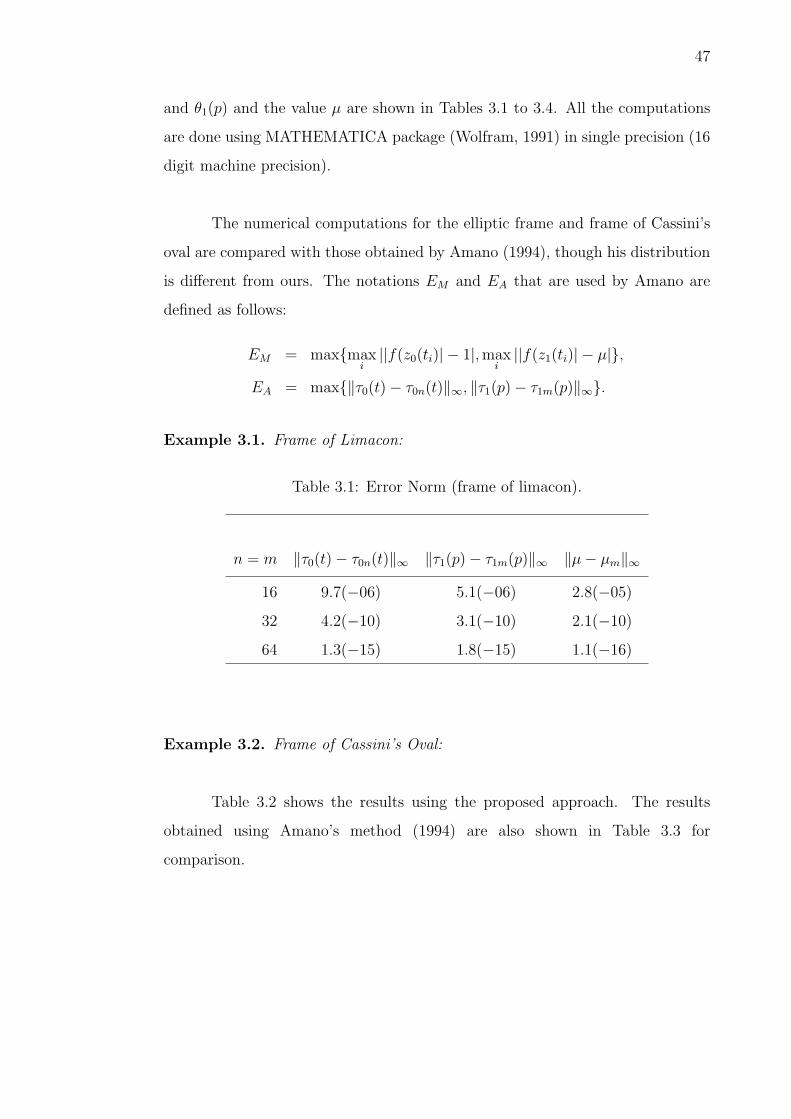
47
and θ1(p) and the value µ are shown in Tables 3.1 to 3.4. All the computations
are done using MATHEMATICA package (Wolfram, 1991) in single precision (16
digit machine precision).
The numerical computations for the elliptic frame and frame of Cassini’s
oval are compared with those obtained by Amano (1994), though his distribution
is different from ours. The notations EM and EA that are used by Amano are
defined as follows:
EM = maxmaxi||f(z0(ti)| − 1|, max
i||f(z1(ti)| − µ|,
EA = max‖τ0(t)− τ0n(t)‖∞, ‖τ1(p)− τ1m(p)‖∞.
Example 3.1. Frame of Limacon:
Table 3.1: Error Norm (frame of limacon).
n = m ‖τ0(t)− τ0n(t)‖∞ ‖τ1(p)− τ1m(p)‖∞ ‖µ− µm‖∞16 9.7(−06) 5.1(−06) 2.8(−05)
32 4.2(−10) 3.1(−10) 2.1(−10)
64 1.3(−15) 1.8(−15) 1.1(−16)
Example 3.2. Frame of Cassini’s Oval:
Table 3.2 shows the results using the proposed approach. The results
obtained using Amano’s method (1994) are also shown in Table 3.3 for
comparison.

48
Table 3.2: Error Norm (frame of Cassini’s Oval) using the proposed method.
n = m ‖τ0(t)− τ0n(t)‖∞ ‖τ1(p)− τ1m(p)‖∞ ‖µ− µm‖∞16 6.4(−03) 2.5(−03) 2.1(−03)
32 6.9(−05) 2.7(−05) 2.1(−05)
64 1.1(−08) 3.7(−09) 3.9(−09)
Table 3.3: Error Norm (frame of Cassini’s oval) using Amano’s method.
n = m EA EM
16 9.7(−03) 9.1(−03)
32 3.8(−04) 3.4(−04)
64 5.0(−07) 6.9(−07)
Example 3.3. Circular Frame:
Table 3.4: Error Norm (circular frame).
n = m ‖τ0(t)− τ0n(t)‖∞ ‖τ1(p)− τ1m(p)‖∞ ‖µ− µm‖∞8 9.8(−11) 4.6(−09) 1.4(−06)
16 8.9(−16) 7.1(−15) 9.5(−11)

49
Example 3.4. Elliptic Frame:
Tables 3.5 and 3.6 shows our results and Amano’s results (1994)
respectively.
Table 3.5: Error Norm (elliptic frame) using the proposed method.
n = m ‖τ0(t)− τ0n(t)‖∞ ‖τ1(p)− τ1m(p)‖∞ ‖µ− µm‖∞16 4.0(−04) 3.2(−04) 3.7(−05)
32 5.1(−06) 1.0(−05) 3.7(−06)
64 2.7(−09) 5.9(−09) 2.2(−09)
128 3.6(−15) 5.8(−15) 1.8(−15)
Table 3.6: Error Norm (elliptic frame) using Amano’s method.
n = m EA EM
16 3.8(−03) 2.8(−02)
32 7.0(−04) 3.2(−03)
64 2.7(−05) 8.4(−05)
CHAPTER 4
AN INTEGRAL EQUATION RELATED TO A BOUNDARY
RELATIONSHIP
4.1 Introduction
Murid et al. (1999) have derived boundary integral equations for conformal
mapping of simply connected region via the Kerzman-Stein and the Neumann
kernels. These integral equations have been used effectively for numerical
conformal mapping. In Chapter 2, the boundary integral equations for conformal
mapping of doubly connected regions via the Kerzman-Stein and the Neumann
kernels have been discussed. These boundary integral equations are the extensions
from those of simply connected region. In this chapter, we focus on improving and
extending the boundary integral equation derived by Murid and Razali (1999) in
Section 2.6.7 to the case of multiply connected regions.
4.2 The Boundary Integral Equation
Let Γ0, Γ1, . . ., ΓM be M +1 smooth Jordan curves in the complex z-plane
such that Γ1, Γ2, . . ., ΓM lies in the interior of Γ0. Denote by Ω the bounded

51
(M + 1)-connected region bounded by Γ0, Γ1, . . ., ΓM . The positive direction of
the contour Γ = Γ0 ∪ Γ1 ∪ · · · ∪ ΓM is usually that for which Ω is on the left as
one traces the boundary (see Figure 2.4).
It is well known that if h is analytic and single-valued in Ω and continuous
on Ω ∪ Γ, we have (Hille, 1973, p. 176)
1
2πi
∫
Γ
h(w)
w − zdw =
1
2h(z), z ∈ Γ. (4.1)
Suppose D(z) is analytic and single-valued with respect to z ∈ Ω and
is continuous on Ω ∪ Γ. Furthermore, suppose that D satisfies the boundary
relationship
D(z) = c(z)
[T (z)Q(z)D(z)
P (z)
]−, z ∈ Γ, (4.2)
where the minus sign in the superscript denotes complex conjugation, T (z) =
z′(t)/|z′(t)| is the complex unit tangent function at z ∈ Γ, while c, P , and Q are
complex-valued functions defined on Γ with the following properties:
(P1) D(z) and P (z) are analytic and single-valued with respect to z ∈ Ω,
(P1) D(z) and P (z) are continuous on Ω ∪ Γ,
(P1) P (z) has a finite number of zeroes at a1, a2, ..., aM in Ω,
(P1) c(z) 6= 0, P (z) 6= 0, Q(z) 6= 0, D(z) 6= 0, z ∈ Γ.
Note that the boundary relationship (4.2) also has the following equivalent
form:
P (z) = c(z)T (z)Q(z)D(z)2
|D(z)|2 , z ∈ Γ. (4.3)
By means of (4.1), an integral equation for D may be constructed that is related
to the boundary relationship (4.2) as shown below:

52
Theorem 4.1
Let u and v be any complex-valued functions that are defined on Γ. Then
1
2
[v(z) +
u(z)
T (z)Q(z)
]D(z) +
PV1
2πi
∫
Γ
[c(z)u(z)
c(w)(w − z)Q(w)− v(z)T (w)
w − z
]D(w)|dw|
= −c(z)u(z)
∑
aj inside Γ
Resw=aj
D(w)
(w − z)P (w)
−
, z ∈ Γ, (4.4)
where the minus sign in the superscript denotes complex conjugation.
Proof. Consider the integral
I1(z) = PV1
2πi
∫
Γ
v(z)T (w)D(w)
w − z|dw|, z ∈ Γ. (4.5)
Using T (w)|d(w)| = dw and (4.1), since D is analytic on Ω, we obtain
I1(z) =1
2v(z)D(z), z ∈ Γ. (4.6)
Next we consider the integral
I2(z) = PV1
2πi
∫
Γ
c(z)u(z)D(w)
c(w)(w − z)Q(w)|dw|, z ∈ Γ. (4.7)
Using the boundary relationship (4.3), |D(w)|2 = D(w)D(w) and T (w)|dw| = dw,
we get
I2(z) = −c(z)u(z)
[1
2πi
∫
Γ
D(w)
(w − z)P (w)dw
]−. (4.8)
Applying the residue theory and formula (4.1) to the integral in (4.8), I2(z)
becomes
I2(z) = −c(z)u(z)
1
2
D(z)
P (z)+
∑
ajinsideΓ
Resw=aj
D(w)
(w − z)P (w)
−
. (4.9)
Applying the boundary relationship (4.2) to the first term on the right-hand side
yields
I2(z) = − u(z)D(z)
2T (z)Q(z)− c(z)u(z)
∑
ajinsideΓ
Resw=aj
D(w)
(w − z)P (w)
−
. (4.10)

53
Finally looking at I2(z)− I1(z), yields
PV1
2πi
∫
Γ
c(z)u(z)D(w)
c(w)(w − z)Q(w)|dw| − PV
1
2πi
∫
Γ
v(z)T (w)D(w)
(w − z)|dw|
= − u(z)D(z)
2T (z)Q(z)− c(z)u(z)
∑
ajinsideΓ
Resw=aj
D(w)
(w − z)P (w)
−
− 1
2v(z)D(z), z ∈ Γ. (4.11)
Rearrangement of (4.11), gives (4.4). This completes the proof. ¥
Remark 1. If P (z) does not have any zeroes in Ω, then the right-hand side
of (4.4) becomes zero.
4.3 Application to Conformal Mapping of Doubly Connected Regions
onto an Annulus via the Kerzman-Stein Kernel
Let w = f(z) be the analytic function which maps the doubly connected
region Ω bounded by the two smooth Jordan curves Γ0 and Γ1 onto the annulus
A = w : µ < |w| < 1 so that Γ0 and Γ1 correspond respectively to |w| = 1
and |w| = µ (see Figure 4.1). As is well known such a mapping function f exists
up to a rotation of the annulus, and the function f could be made unique by
prescribing that
f(a) = 0, f ′(a) > 0 or f(z∗) = 1, (4.12)
where a ∈ Ω and z∗ ∈ Γ0 are fixed points.
The boundary values of f can be represented in the form
f(z0(t)) = eiθ0(t), Γ0 : z = z0(t), 0 ≤ t ≤ β0, (4.13)
f(z1(t)) = µeiθ1(t), Γ1 : z = z1(t), 0 ≤ t ≤ β1, (4.14)

54
1!
"z*
0!#
"1
Figure 4.1: Mapping of a doubly connected region Ω onto an annulus.
where θ0(t) and θ1(t) are the boundaries correspondence functions of Γ0 and Γ1
respectively.
The unit tangent to Γ at z(t) is denoted by T (z(t)) = z′(t)/|z′(t)|. Thus
it can be shown that
f(z0(t)) =1
iT (z0(t))
θ′0(t)|θ′0(t)|
f ′(z0(t))
|f ′(z0(t))| =1
iT (z0(t))
f ′(z0(t))
|f ′(z0(t))| , z0 ∈ Γ0, (4.15)
f(z1(t)) =µ
iT (z1(t))
θ′1(t)|θ′1(t)|
f ′(z1(t))
|f ′(z1(t))| =µ
iT (z1(t))
f ′(z1(t))
|f ′(z1(t))| , z1 ∈ Γ1. (4.16)
The boundary relationships (4.15) and (4.16) can be unified as
f(z) =|f(z)|
iT (z)
f ′(z)
|f ′(z)| , z ∈ Γ. (4.17)
Note that the values of |f(z)| is either 1 or µ for z ∈ Γ = Γ0 ∪ Γ1. Also
note that since f ′(z) is different from 0 and analytic in Ω ∪ Γ, thus an analytic
square root, denoted by√
f ′(z), may be defined on Ω ∪ Γ. Comparing (4.17)
with (4.3) leads to a choice of c(z) = i|f(z)|, P (z) = f(z), D(z) =√
f ′(z),
Q(z) = 1, u(z) = T (z)Q(z) and v(z) = 1. With these assignments, Theorem 4.1
and Remark 1, imply
√f ′(z) + PV
1
2πi
∫
Γ
[|f(z)|T (z)
|f(w)|(w − z)− T (w)
(w − z)
] √f ′(w)|dw| = 0, z ∈ Γ.
(4.18)

55
Note that (4.18) does not posses a unique solution. If f(z) satisfies (4.18),
then so is reiαf(z), i.e.
√[reiαf(z)]′ + PV
1
2πi
∫
Γ
[|reiαf(z)|T (z)
|reiαf(w)|(w − z)− T (w)
(w − z)
]√[reiαf(w)]′|dw| = 0,
z ∈ Γ, (4.19)
for any real constant r > 0 and α.
To achieve uniquenee, several condition need to be imposed. Suppose
F (z) = reiαf(z), r, α ∈ < (4.20)
is a mapping function that maps a doubly connected regions onto an annulus
A = w : rµ < |w| < r. The Arg(F (z)) and Arg(f(z)) differ by α.
As is well known such a mapping function F (z) exists up to a rotation
and the rotation could be fixed by prescribing F (z∗) = r, where z∗ ∈ Γ0 is fixed
point.
1z*
0
1
r r
f(z)
F(z)=rei
f(z)
Figure 4.2: Mapping of doubly connected region onto an annulus
The equation (4.20) with z = z∗ implies
F (z∗) = reiαf(z∗) = r,

56
and Figure 4.2 implies
Re [F ′(z∗)] = 0,
Im [F ′(z∗)] > 0.(4.21)
Note that
F ′(z∗) = reiαf ′(z∗)
= reiα(Re f ′(z∗) + i Im f ′(z∗))
= −r sin α Im f ′(z∗) + i r cos α Im f ′(z∗). (4.22)
Applying the condition in (4.21), we obtain
sin α Im f ′(z∗) = 0,
cos α Im f ′(z∗) > 0,
which admit the solution α = 0 since Im f ′(z∗) > 0. Thus α is now fixed.
So the equation (4.20) becomes
F (z) = rf(z). (4.23)
To fix r, we observe that
F (z0(t)) = reiθ0(t), z0(t) ∈ Γ0. (4.24)
Differentiating and taking modulus on both sides of equation (4.24), we obtain
|F ′(z0(t))z′0(t)| = |riθ′0(t)eiθ0(t)| = |θ′0(t)|. (4.25)
The boundary correspondence function θ0(t) is an increasing monotone function
and it’s derivative is positive, we have |θ′0(t)| = θ′0(t). Thus, integrating (4.25)
with respect to t to 2π gives
∫ 2π
0
|F ′(z0(t))z′0(t)|dt = |r|
∫ 2π
0
θ′0(t)dt = 2π|r|,

57
Setting the condition ∫ 2π
0
|F ′(z0(t))z′0(t)|dt = 2π,
implies r = 1. Hence F (z) = f(z).
The integral equation (4.18) can also be written briefly as
√f ′(z) +
∫
Γ
A∗(z, w)√
f ′(w)|dw| = 0, z ∈ Γ, (4.26)
where
A∗(z, w) =1
2πi
[|f(z)|T (z)
|f(w)|(w − z)− T (w)
(w − z)
].
This result has already been given in Chapter 3 but the derivation
presented here is much simpler. The integral equation will be used in Section
5.2, Chapter 5 for the numerical conformal mapping of doubly connected region
onto an annulus with some normalizing conditions different from Chapter 3.
4.4 Application to Conformal Mapping of Multiply Connected
Regions onto an Annulus with Circular Slits via the Neumann
Kernel
This section gives an application of Theorem 4.1 to conformal mapping of
multiply connected region Ω of connectivity M +1. Let w = f(z) be the analytic
function which maps Ω conformally onto an annulus (µ1 < |w| < 1) with circular
slits of radii µ2 < 1, ..., µM < 1 (see Figure 4.3). The mapping function f is
determined up to a rotation of the annulus. The function f could be made unique
by prescribing (4.12).
The boundary values of f can be represented in form
f(z0(t)) = eiθ0(t), Γ0 : z = z0(t), 0 ≤ t ≤ β0, (4.27)
f(zp(t)) = µpeiθp(t), Γp : z = zp(t), 0 ≤ t ≤ βp, p = 1, 2, ..., M, (4.28)

58
1
M! 2!1!"#
$1 $2
$M
$0
" z*
Figure 4.3: Mapping of a multiply connected region Ω of connectivity M +1 onto
an annulus with circular slits.
where θ0(t), θ1(t), ..., θM(t) are the boundaries correspondence functions of Γ0, Γ1,
..., ΓM respectively.
The unit tangent to Γ at z(t) is denoted by T (z(t)) = z′(t)/|z′(t)|. Thus
it can be shown that
f(z0(t)) =1
iT (z0(t))
θ′0(t)|θ′0(t)|
f ′(z0(t))
|f ′(z0(t))| =1
iT (z0(t))
f ′(z0(t))
|f ′(z0(t))| , z0 ∈ Γ0,
(4.29)
f(z1(t)) =µ1
iT (z1(t))
θ′1(t)|θ′1(t)|
f ′(z1(t))
|f ′(z1(t))| =µ1
iT (z1(t))
f ′(z1(t))
|f ′(z1(t))| , z1 ∈ Γ1,
(4.30)
f(zp(t)) =µp
iT (zp(t))
θ′p(t)
|θ′p(t)|f ′(zp(t))
|f ′(zp(t))| = ±µp
iT (zp(t))
f ′(zp(t))
|f ′(zp(t))| , zp ∈ Γp,
(4.31)
for p = 2, ..., M. If M = 1, then relationship (4.31) does not exist; i.e., only (4.29)
and (4.30) hold. Note that θ′0(t) > 0 and θ′1(t) > 0 while θ′p(t) may be positive
or negative since each circular slit f(Γp) is traversed twice (see Figure 4.3). Thus
θ′p(t)/|θ′p(t)| = ±1.
The boundary relationships (4.29), (4.30) and (4.31) can be unified as
f(z) = ±|f(z)|i
T (z)f ′(z)
|f ′(z)| , z ∈ Γ, (4.32)

59
where Γ = Γ0 ∪ Γ1 ∪ · · · ∪ ΓM . Note that the value of |f(z)| is either 1, µ1 or
µp for z ∈ Γ. However we cannot compare (4.32) with (4.3) due to the presence
of the ± sign. To overcome this problem, we square both sides of the boundary
relationship (4.32) to get
f(z)2 = −|f(z)|2T (z)2 f ′(z)2
|f ′(z)|2 , z ∈ Γ. (4.33)
Comparison of (4.3) and (4.33) leads to a choice of c(z) = −|f(z)|2, P (z) =
f(z)2, D(z) = f ′(z), Q(z) = T (z), u(z) = T (z)Q(z) and v(z) = 1. Substituting
these assignments into (4.4) leads to an integral equation satisfied by f ′(z), i.e.,
f ′(z) + PV1
2πi
∫
Γ
[|f(z)|2T (z)2
|f(w)|2(w − z)T (w)− T (w)
(w − z)
]f ′(w)|dw|
= |f(z)|2T (z)2
∑
ajinsideΓ
Resw=aj
f ′(w)
(w − z)f(w)2
−
, z ∈ Γ. (4.34)
For the case where Ω is a multiply connected regions being mapped onto
an annulus with concentric circular slits, f(z) does not have any zeroes in Ω. Thus
the right-hand side of (4.34) vanishes and the integral equation (4.34) becomes
f ′(z) + PV1
2πi
∫
Γ
[|f(z)|2T (z)2
|f(w)|2(w − z)T (w)− T (w)
(w − z)
]f ′(w)|dw| = 0, z ∈ Γ.
(4.35)
Multiply both sides by T (z) and using the fact T (z)T (z) = |T (z)|2 = 1 gives
T (z)f ′(z) + PV1
2πi
∫
Γ
[|f(z)|2T (z)
|f(w)|2(w − z)− T (z)
(w − z)
]T (w)f ′(w)|dw| = 0,
z ∈ Γ. (4.36)
Note that (4.36) does not posses a unique solution. If f(z) satisfies (4.36),
then so is reiαf(z), i.e.
T (z)[reiαf(z)]′
+ PV1
2πi
∫
Γ
[|reiαf(z)|2T (z)
|reiαf(w)|2(w − z)− T (z)
(w − z)
]T (w)[reiαf(w)]′|dw| = 0,
z ∈ Γ. (4.37)
60
for any real constants r > 0 and α.
Suppose
F (z) = reiαf(z), r, α ∈ < (4.38)
is a mapping function that maps a multiply connected regions onto an annulus
(rµ1 < |w| < r) with circular slits of radii rµ2 < r, ..., rµM < 1 and the Arg(F (z))
and Arg(f(z)) differ by α. As is well known such a mapping function F (z) exists
up to a rotation and the rotation could be fixed by prescribing F (z∗) = f , where
z∗ ∈ Γ0 is fixed point. Using the same ideas presented in Section 4.3, imposing
the conditions
sin α Im f ′(z∗) = 0,
cos α Im f ′(z∗) > 0,∫ 2π
0
|F ′(z0(t))z′0(t)|dt = 2π,
lead to α = 0 and r = 1. Hence F (z) = f(z).
The integral equation (4.36) can also be written briefly as
g(z) +
∫
Γ
N∗(z, w)g(w)|dw| = 0, z ∈ Γ, (4.39)
where
g(z) = T (z)f ′(z),
N∗(z, w) =1
2πi
[T (z)
(z − w)− |f(z)|2T (z)
|f(w)|2(z − w)
]. (4.40)
This integral equation will be used in Sections 5.3 and 5.4 for the numerical
conformal mapping of doubly connected region onto an annulus and triply
connected region onto an annulus with a slit.
Comparing (4.3) and (4.33) yields still another possible assignments, i.e.,
c(z) = −1, P (z) = 1, D(z) = f ′(z)/f(z) and Q(z) = T (z).

61
Application of Theorem 4.4 with Remark 1 to these assignments, along with the
choice of u(z) = T (z)Q(z) and v(z) = 1, gives
f ′(z)
f(z)+ PV
1
2πi
∫
Γ
[T (z)2
(w − z)T (w)− T (w)
(w − z)
]f ′(w)
f(w)|dw| = 0, z ∈ Γ. (4.41)
If we multiply both sides of (4.41) by T (z), we obtain
T (z)f ′(z)
f(z)+ PV
1
2πi
∫
Γ
[T (z)
(w − z)− T (z)
(w − z)
]T (w)
f ′(w)
f(w)|dw| = 0, z ∈ Γ.
(4.42)
The integral equation (4.42) can also be written briefly as
Φ(z) +
∫
Γ
N(z, w)Φ(w)|dw| = 0, z ∈ Γ, (4.43)
where Φ(z) = T (z)f ′(z)/f(z) and N is again the Neumann kernel (2.22).
From (4.27) and (4.28), we see that
f ′(z0(t))z′0(t) = iθ′0(t)e
iθ0(t) = if(z0(t))θ′0(t), 0 ≤ t ≤ β0, (4.44)
f ′(zp(t))z′p(t) = iµpθ
′p(t)e
iθp(t) = if(zp(t))θ′p(t), 0 ≤ t ≤ βp. (4.45)
In other words,
f ′(z(τ))z′(τ) = if(z(τ))θ′(τ), z(τ) ∈ Γ, 0 ≤ τ ≤ β,
which implies
f ′(z(τ))
f(z(τ))z′(τ) = iθ′(τ), z(τ) ∈ Γ, 0 ≤ τ ≤ β.
Substituting this result into (4.43) and using the definition that T (z(τ)) =
z′(τ)/|z′(τ)|, we get
θ′(τ) +
∫ β
0
k(τ, σ)θ′(σ)dσ = 0, 0 ≤ τ ≤ β, (4.46)

62
where
k(τ, σ) = |z′(τ)|N(z(τ), z(σ)) =
1
πIm
[z′(τ)
z(τ)− z(σ)
], if τ 6= σ,
1
2πIm
[z′′(t)z′(τ)
], if τ = σ.
For doubly connected regions, the integral equation (4.46) is also known
as the Warschawski’s equation (see Section 2.6.6).
4.5 Application to Conformal Mapping of Multiply Connected
Regions onto a Disk with Circular Slits via the Neumann Kernel
This section gives an application of Theorem 4.1 to conformal mapping
of multiply connected region Ω of connectivity M + 1 onto a disk with circular
slits. Let w = f(z) be the analytic function which maps Ω conformally onto a
disk |w| < r with circular slits of radii µpr, where 0 < µp < 1, p = 1, 2, ..., M (see
Figure 4.4). The function f could be made unique by prescribing (4.12).
!!!
"1 "2
"M
!!!
r#M r#2r#1$
r
"0
$ z*
Figure 4.4: Mapping of a multiply connected region Ω of connectivity M +1 onto
a disk with circular slits.

63
The boundary values of f can be represented in form
f(z0(t)) = reiθ0(t), Γ0 : z = z0(t), 0 ≤ t ≤ β0, (4.47)
f(zp(t)) = µpreiθp(t), Γp : z = zp(t), 0 ≤ t ≤ βp, p = 1, 2, ...,M, (4.48)
where θ0(t), θ1(t), ..., θM(t) are the boundaries correspondence functions of Γ0,
Γ1, ..., ΓM respectively.
Thus it can be shown that
f(z0(t)) =r
iT (z0(t))
θ′0(t)|θ′0(t)|
f ′(z0(t))
|f ′(z0(t))| =r
iT (z0(t))
f ′(z0(t))
|f ′(z0(t))| , z0 ∈ Γ0, (4.49)
f(zp(t)) =µpr
iT (zp(t))
θ′p(t)
|θ′p(t)|f ′(zp(t))
|f ′(zp(t))| = ±µpr
iT (zp(t))
f ′(zp(t))
|f ′(zp(t))| , zp ∈ Γp,
(4.50)
for p = 1, 2, ..., M . Note that θ′0(t) > 0 while θ′p(t) may be positive or negative
since the circular slit f(Γp) is traversed twice. Thus θ′p(t)/|θ′p(t)| = ±1.
The boundary relationships (4.49) and (4.50) can be unified as
f(z) = ±|f(z)|i
T (z)f ′(z)
|f ′(z)| , z ∈ Γ, (4.51)
where Γ = Γ0 ∪ Γ1 ∪ · · · ∪ ΓM . Note that the value of |f(z)| is either r or µpr for
z ∈ Γ. Squaring both sides of the boundary relationship (4.51) gives
f(z)2 = −|f(z)|2T (z)2 f ′(z)2
|f ′(z)|2 , z ∈ Γ. (4.52)
Comparing (4.52) with (4.3), leads to a choice of c(z) = −|f(z)|2, P (z) =
f(z)2, D(z) = f ′(z), Q(z) = T (z), u(z) = T (z)Q(z) and v(z) = 1. Substituting
these assignments into (4.4) leads to an integral equation satisfied by f ′(z), i.e.,
f ′(z) + PV1
2πi
∫
Γ
[|f(z)|2T (z)2
|f(w)|2(w − z)T (w)− T (w)
(w − z)
]f ′(w)|dw|
= |f(z)|2T (z)2
∑
ajinsideΓ
Resw=aj
f ′(w)
(w − z)f(w)2
−
, z ∈ Γ. (4.53)

64
To evaluate the residue in equation (4.53) we use the fact that if f(w) =
g(w)/h(w) where g and h are analytic at a, and g(a) 6= 0, h(a) = h′(a) = 0,
h′′(a) 6= 0, which means a is a double pole of f(w), then (Gonzalez, 1992)
Resw=a
f(w) = 2g′(a)
h′′(a)− 2
3
h′′′(a)g(a)
h′′(a)2. (4.54)
Applying (4.54) to the residue in (4.53) and after several algebraic manipulations,
we obtain
Resw=a
f ′(w)
(w − z)f(w)2= − 1
(a− z)2f ′(a). (4.55)
Thus integral equation (4.53) becomes
f ′(z) + PV1
2πi
∫
Γ
[|f(z)|2T (z)2
|f(w)|2(w − z)T (w)− T (w)
(w − z)
]f ′(w)|dw|
= −|f(z)|2 T (z)2
(a− z)2f ′(a), z ∈ Γ. (4.56)
Multiply both sides of the equation by f ′(a)T (z) and use the fact that T (z)T (z) =
|T (z)|2 = 1 gives
f ′(a)T (z)f ′(z)
+ PV1
2πi
∫
Γ
[|f(z)|2T (z)
|f(w)|2(w − z)− T (z)
(w − z)
]f ′(a)T (w)f ′(w)|dw|
= −|f(z)|2 T (z)
(a− z)2, z ∈ Γ. (4.57)
Equation (4.57) can also be written as
g(z, a) +
∫
Γ
N∗(z, w)g(w, a)|dw| = |f(z)|2h(a, z), z ∈ Γ. (4.58)
where the kernel N∗ is as given in (4.40) and
g(z, a) = f ′(a)T (z)f ′(z),
h(a, z) = − T (z)
(a− z)2.
This integral equation will be used in Chapter 6 for the numerical
conformal mapping of multiply connected regions onto a disk with slits.
CHAPTER 5
NUMERICAL CONFORMAL MAPPING OF MULTIPLY
CONNECTED REGIONS ONTO AN ANNULUS WITH
CIRCULAR SLITS
5.1 Introduction
We have discussed in Chapter 4 the theoretical aspects of constructing
some integral equations for conformal mapping of doubly connected region onto
an annulus via the Kerzman-Stein kernel and conformal mapping of multiply
connected regions onto an annulus with circular slits via the Neumann kernel.
In this chapter, we shall discuss the numerical aspects of conformal mapping of
multiply connected regions based on the integral equation developed in Chapter
4.
5.2 Conformal Mapping of Doubly Connected Regions onto an
Annulus via the Kerzman-Stein Kernel
5.2.1 A System of Integral Equations
Suppose Ω is a doubly connected region bounded by Γ0 and Γ1 as shown
in Figure 4.1. Since Ω is a doubly connected region, the single integral equation

66
in (4.26) can be separated into a system of equations
η(z0) +
∫
Γ0
A(z0, w)η(w)|dw| −∫
−Γ1
P (z0, w)η(w)|dw| = 0, z0 ∈ Γ0, (5.1)
η(z1) +
∫
Γ0
Q(z1, w)η(w)|dw| −∫
−Γ1
A(z1, w)η(w)|dw| = 0, z1 ∈ Γ1, (5.2)
where
η(z) =√
f ′(z),
P (z, w) =1
2πi
[T (z)
µ(w − z)− T (w)
(w − z)
],
Q(z, w) =1
2πi
[µT (z)
(w − z)− T (w)
(w − z)
],
A(z, w) =
H(w, z)−H(z, w), w, z ∈ Γ, w 6= z,
0, w = z ∈ Γ,
H(w, z) =1
2πi
T (z)
(z − w), w ∈ Ω ∪ Γ, z ∈ Γ, w 6= z.
The kernel A is known as the Kerzman-Stein kernel (Kerzman and
Trummer, 1986) and is smooth and skew-Hermitian. The kernel H is usually
referred to as the Cauchy kernel. The integral equations (5.1) and (5.2) involve
the unknown parameter µ. To obtain a unique solution, we first consider applying
the condition f(z0(0)) = 1. For the test regions that we have chosen, the
unit tangent vector T (z0(0)) is equal to i. From equation (4.15), this implies
η(z0(0))2/|η(z0(0))|2 = 1, which means
Re [η(z0(0))2/|η(z0(0)|2] = 1, (5.3)
Im [η(z0(0))2] = 0. (5.4)
Next we consider equation (4.13), which upon differentiation and taking
modulus on both sides, gives
|f ′(z0(t))z′0(t)| = |eiθ0(t)iθ′0(t)| = |θ′0(t)|. (5.5)
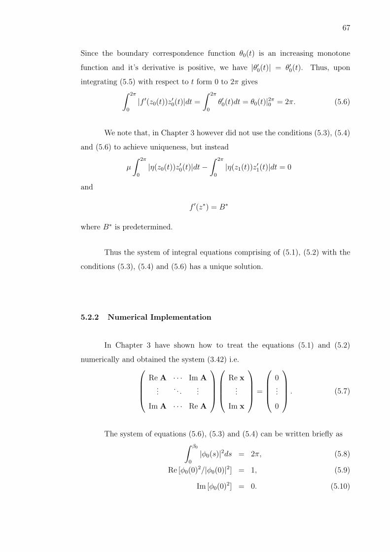
67
Since the boundary correspondence function θ0(t) is an increasing monotone
function and it’s derivative is positive, we have |θ′0(t)| = θ′0(t). Thus, upon
integrating (5.5) with respect to t form 0 to 2π gives∫ 2π
0
|f ′(z0(t))z′0(t)|dt =
∫ 2π
0
θ′0(t)dt = θ0(t)|2π0 = 2π. (5.6)
We note that, in Chapter 3 however did not use the conditions (5.3), (5.4)
and (5.6) to achieve uniqueness, but instead
µ
∫ 2π
0
|η(z0(t))z′0(t)|dt−
∫ 2π
0
|η(z1(t))z′1(t)|dt = 0
and
f ′(z∗) = B∗
where B∗ is predetermined.
Thus the system of integral equations comprising of (5.1), (5.2) with the
conditions (5.3), (5.4) and (5.6) has a unique solution.
5.2.2 Numerical Implementation
In Chapter 3 have shown how to treat the equations (5.1) and (5.2)
numerically and obtained the system (3.42) i.e.
Re A · · · Im A...
. . ....
Im A · · · Re A
Re x...
Im x
=
0...
0
. (5.7)
The system of equations (5.6), (5.3) and (5.4) can be written briefly as∫ β0
0
|φ0(s)|2ds = 2π, (5.8)
Re [φ0(0)2/|φ0(0)|2] = 1, (5.9)
Im [φ0(0)2] = 0. (5.10)

68
where
φ0(t) = |z′0(t)|1/2η(z0(t)),
φ1(t) = |z′1(t)|1/2η(z1(t)).
Since φ = Re φ + i Im φ, equations (5.8), (5.9) and (5.10) become
n∑j=1
((Re x0j)2 + (Im x0j)
2) = n, (5.11)
Re [x201/((Re x01)
2 + (Im x01)2)] = 1, (5.12)
Im x201 = 0. (5.13)
Therefore, the real nonlinear system in (5.7) can be solved simultaneously with
the equations (5.11), (5.12) and (5.13) which also involves the Re and Im parts of
the unknown functions. This system is an over-determined system of nonlinear
equations involving 2(n + m) + 3 equations in 2(n + m) + 1 unknowns. As in
Chapter 3, we also use Gauss-Newton method to solve this nonlinear least square
problem.
5.2.3 Numerical Results
For our numerical experiments, we have used three test regions i.e. frame
of Cassini’s oval, ellipse/circle and elliptical domain with circular hole. The exact
boundary correspondence function for Cassini’s oval is discussed in Section 2.5.5.
All the computations are done using MATHEMATICA package (Wolfram, 1991)
in single precision (16 digit machine precision). We also show the comparisons
of our numerical computations for the test regions with with those obtained
by Amano (1994), Ellacott (1979), Papamicheal and Warby (1984) and Symm
(1969).

69
Example 5.1. Frame of Cassini’s Oval:
Let
Γ0 : z(t) =
√b20 cos 2t +
√a4
0 − b40 sin2 2t eit, a0 > 0, b0 > 0,
Γ1 : z(t) =
√b21 cos 2t +
√a4
1 − b41 sin2 2t eit, a1 > 0, b1 > 0, 0 ≤ t ≤ 2π.
The exact mapping function is
f(z) =a0z√
b20z
2 + a40 − b4
0
, µ =a0b1
a1b0
.
Figure 5.1 shows the region and image based on our method. The results
for the sub-norm error between the exact values of θ0(t), θ1(t), µ and their
corresponding approximations θ0n(t), θ1n(t), µn are shown in Table 4.1. Table
4.2 shows the results obtained in Chapter 3 with different normalizing conditions
from ours. Table 4.3 shows the results calculated by Amano (1994) and Symm
(1969), though their distributions are different from ours. The notations EM and
EA that are used by Amano or Symm are defined as follows:
EM = maxmaxi||f(z0(ti))| − 1|, max
i||f(z1(ti))| − µ|, (5.14)
EA = max‖θ0(t)− θ0n(t)‖∞, ‖θ1(t)− θ1n(t)‖∞. (5.15)
-10 -5 5 10
-4
-2
2
4
-1 -0.5 0.5 1
-1
-0.5
0.5
1
Figure 5.1: Frame of Cassini’s Oval with a0 = 2√
14, a1 = 2, b0 = 7, and b1 = 1.

70
Table 5.1: Error norm (frame of Cassini’s oval) using our method
n = m minimal S(x) ‖θ0(t)− θ0n(t)‖∞ ‖θ1(t)− θ1n(t)‖∞ ‖µ− µn‖∞16 8.4(−31) 6.4(−03) 2.5(−03) 2.1(−03)
32 8.4(−30) 6.9(−05) 2.7(−05) 2.1(−05)
64 5.5(−30) 1.1(−08) 4.1(−09) 3.1(−09)
128 3.4(−28) 2.7(−15) 8.9(−16) 1.1(−16)
Table 5.2: Error norm (frame of Cassini’s oval) in Chapter 3 with different
conditions
n = m ‖θ0(t)− θ0n(t)‖∞ ‖θ1(t)− θ1n(t)‖∞ ‖µ− µn‖∞16 6.4(−03) 2.5(−03) 2.1(−03)
32 6.9(−05) 2.7(−05) 2.1(−05)
64 1.1(−08) 3.7(−09) 3.9(−09)
Table 5.3: Error Norm (frame of Cassini’s oval) using Amano’s method and
Symm’s method
Amano’s Method Symm’s Method
n = m EM EA n = m EM
16 9.1(−03) 9.7(−03) 64 1.94(−02)
32 3.4(−04) 3.8(−04) 128 3.00(−03)
64 6.9(−07) 5.0(−08) 256 7.00(−04)
128 7.7(−11) 7.7(−11)
Example 5.2. Ellipse/Circle:
Let
Γ0 : z(t) = 2 cos t + i sin t,
Γ1 : z(t) = 0.5 (cos t + i sin t), 0 ≤ t ≤ 2π.

71
We have adopted this example problem from Ellacott (1979) with µE =
0.4141 for comparison. See Table 4.4 for radius comparisons. Figure 5.2 shows
the region and its image based on our method.
-2 -1 1 2
-1
-0.5
0.5
1
-1 -0.5 0.5 1
-1
-0.5
0.5
1
Figure 5.2: Conformal mapping ellipse/circle onto an annulus
Table 5.4: The radius comparison for ellipse/circle
minimal Radius Comparison Value of
n = m S(x) µ− µE µ
8 3.0(−31) 2.7(−02) 0.441484
16 4.9(−30) 3.8(−04) 0.4144811
32 4.2(−30) 2.0(−05) 0.4141199465
64 9.3(−28) 2.0(−05) 0.414119807860853
Example 5.3. Elliptical Region with Circular Hole:
Let
Γ0 = (x, y) : (x +1
2a0)
2/a20 + y2 = 1,
Γ1 = (x, y) : x2 + y2 =1
9a2
0, 1 < a0 ≤ 2.
We have adopted this example problem from Papamichael and Warby
(1984) for comparison of µ. Since the conditions of the problem are somewhat
different, A = w : µ < |w| < 1 in ours and a = w : 1 < |w| < M in Papamichael
and Warby (1984), our radius µ should be multiplied by M for comparison (See
72
Table 4.5). In Table 4.6, we list the computed approximations of µ based on
our method and the computed approximations to the modulus M based on
Papamichael and Warby method. The notation EN that is used by Papamichael
and Warby is defined as
EN = maxmaxi||f(z0(ti))| −M ||, max
i||f(z1(ti))| − 1||, (5.16)
Figure 5.3 shows the region and its image based on our method.
-3 -2 -1 1
-1
-0.5
0.5
1
-1 -0.5 0.5 1
-1
-0.5
0.5
1
Figure 5.3: Conformal mapping elliptical region with circular hole onto an annulus
with a0 = 0.20.
Table 5.5: The computed approximations of µ and M for elliptical region with
circular hole
Our Method Papamichael and Warby Method
a0 µ M 1/M
1.04 0.4803797010421916 2.081686628 0.4803797010315426
1.08 0.4869154853494373 2.053744500 0.4869154853488348
1.20 0.5080480086200778 1.968317921 0.5080480085716803
1.40 0.5480734581257742 1.824572938 0.5480734582724585
1.60 0.5938360511745354 1.683966719 0.5938359640467455
1.80 0.6455396040618700 1.549091634 0.6455396040180280
2.00 0.7043817963286256 1.419684616 0.7043817963017217

73
Table 5.6: The radius comparison for elliptical region with circular hole
a0 n = m minimal S(x) ‖µ− 1/M‖∞ n = m EN
1.04 32 4.6(−29) 2.0(−06) 31 2.1(−05)
1.08 32 8.4(−31) 1.4(−06) 31 8.7(−06)
1.20 32 5.2(−30) 3.0(−07) 29 7.5(−08)
1.40 32 1.4(−29) 1.9(−08) 29 2.0(−06)
1.60 32 3.7(−29) 2.4(−06) 25 3.2(−05)
1.80 32 1.3(−29) 3.5(−05) 23 3.9(−04)
2.00 32 2.3(−29) 1.1(−04) 27 2.0(−03)
5.3 Conformal Mapping of Doubly Connected Regions onto an
Annulus via the Neumann Kernel
5.3.1 A System of Integral Equations
Suppose Ω is a doubly connected region bounded by Γ0 and Γ1 (see Figure
4.3 with M = 1). For the special case where Ω is a doubly connected region, the
single integral equation in (4.39) can be separated into a system of equations
g(z0) +
∫
Γ0
N(z0, w)g(w)|dw| −∫
−Γ1
P0(z0, w)g(w)|dw| = 0, z0 ∈ Γ0, (5.17)
g(z1) +
∫
Γ0
P1(z1, w)g(w)|dw| −∫
−Γ1
N(z1, w)g(w)|dw| = 0. z1 ∈ Γ1, (5.18)
where
g(z) = T (z)f ′(z),
P0(z, w) =1
2πi
[T (z)
(z − w)− T (z)
µ21(z − w)
],
P1(z, w) =1
2πi
[T (z)
(z − w)− µ2
1T (z)
(z − w)
],
N(z, w) =
1
πIm
[T (z)
z − w
], if w, z ∈ Γ, w 6= z,
1
2π
Im[z′′(t)z′(t)]|z′(t)|3 , if w = z ∈ Γ.

74
The kernel N is also known as the Neumann kernel (Henrici, 1974).
Note that the PV symbols are no longer required in (5.17) and (5.18) since
the integrands are continuous along their respective paths of integrations. The
integral equations (5.17) and (5.18) also involve the unknown parameter µ1.
Naturally it is also required that the unknown mapping function f(z) be single-
valued in the problem domain (Henrici, 1974, p. 217), i.e.,∫
−Γ1
f ′(w)dw = 0 (5.19)
which implies ∫
−Γ1
g(w)|dw| = 0. (5.20)
Note that the system of integral equations consisting of (5.17), (5.18) and
(5.20) is homogeneous and does not have a unique solution. To obtain a unique
solution, we need to impose some conditions on g(z). First, we consider applying
the condition f(z0(0)) = 1. From (4.29), this implies g(z0(0))/|g(z0(0))| = i,
which means
Re [g(z0(0))] = 0, (5.21)
Im [g(z0(0))/|g(z0(0)|] = 1. (5.22)
Next we consider equations (4.27) and (4.28). Upon differentiation and
taking modulus to both sides of equations (4.27) and (4.28), gives
|T (z0(t))f′(z0(t))z
′0(t)| = |T (z0(t))e
iθ0(t)iθ′0(t)| = |θ′0(t)|. (5.23)
|T (z1(t))f′(z1(t))z
′1(t)| = |T (z1(t))µ1e
iθ1(t)iθ′1(t)| = µ1|θ′1(t)|. (5.24)
Since the boundary correspondence functions θ0(t) and θ1(t) are increasing
monotone functions, their derivatives are positive which implies |θ′0(t)| = θ′0(t)
and |θ′1(t)| = θ′1(t). Upon integrating (5.23) and (5.24) with respect to t form 0
to 2π gives∫ 2π
0
|g(z0(t))z′0(t)|dt =
∫ 2π
0
θ′0(t)dt = θ0(t)|2π0 = 2π, (5.25)
∫ 2π
0
|g(z1(t))z′1(t)|dt = µ1
∫ 2π
0
θ′1(t)dt = µ1θ1(t)|2π0 = µ12π. (5.26)

75
Thus the system of integral equations comprising of (5.17), (5.18), (5.20)
with the conditions (5.21), (5.22), (5.25) and (5.26) has a unique solution.
5.3.2 Numerical Implementation
Suppose Γ0 and Γ1 be given in parametric representations as follows:
Γ0 : z = z0(t), 0 ≤ t ≤ β0,
Γ1 : z = z1(t), 0 ≤ t ≤ β1.
Then the system of integral equations (5.17), (5.18), (5.20), (5.25) and (5.26)
become
g(z0(t)) +
∫ β0
0
N(z0(t), z0(s))g(z0(s))|z′0(s)|ds
−∫ β1
0
P0(z0(t), z1(s))g(z1(s))|z′1(s)|ds = 0, z0(t) ∈ Γ0, (5.27)
g(z1(t)) +
∫ β0
0
P1(z1(t), z0(s))g(z0(s))|z′0(s)|ds
−∫ β1
0
N(z1(t), z1(s))g(z1(s))|z′1(s)|ds = 0, z1(t) ∈ Γ1, (5.28)
∫ β1
0
g(z1(s))|z′1(s)|ds = 0, (5.29)
∫ β0
0
|g(z0(s))z′0(s)|ds = 2π, (5.30)
∫ β1
0
|g(z1(s))z′1(s)|ds = 2πµ1. (5.31)
Multiply (5.27) and (5.28) respectively by |z′0(t)| and |z′1(t)| gives
|z′0(t)|g(z0(t)) +
∫ β0
0
|z′0(t)|N(z0(t), z0(s))g(z0(s))|z′0(s)|ds
−∫ β1
0
|z′0(t)|P0(z0(t), z1(s))g(z1(s))|z′1(s)|ds = 0, z0(t) ∈ Γ0, (5.32)
|z′1(t)|g(z1(t)) +
∫ β0
0
|z′1(t)|P1(z1(t), z0(s))g(z0(s))|z′0(s)|ds
−∫ β1
0
|z′1(t)|N(z1(t), z1(s))g(z1(s))|z′1(s)|ds = 0, z1(t) ∈ Γ1. (5.33)

76
Defining
φ0(t) = |z′0(t)|g(z0(t)),
φ1(t) = |z′1(t)|g(z1(t)),
K00(t0, s0) = |z′0(t)|N(z0(t), z0(s)),
K01(t0, s1) = |z′0(t)|P0(z0(t), z1(s)),
K10(t1, s0) = |z′1(t)|P1(z1(t), z0(s)),
K11(t1, s1) = |z′1(t)|N(z1(t), z1(s)),
the system of equations (5.32), (5.33), (5.29), (5.30), (5.31), (5.21) and (5.22) can
be briefly written as
φ0(t) +
∫ β0
0
K00(t0, s0)φ0(s)ds−∫ β1
0
K01(t0, s1)φ1(s)ds = 0, (5.34)
φ1(t) +
∫ β0
0
K10(t1, s0)φ0(s)ds−∫ β1
0
K11(t1, s1)φ1(s)ds = 0, (5.35)
∫ β1
0
φ1(s)ds = 0, (5.36)
∫ β0
0
|φ0(s)|ds = 2π, (5.37)
∫ β1
0
|φ1(s)|ds = 2πµ1, (5.38)
Re φ0(0) = 0, (5.39)
Im [φ0(0)/|φ0(0)|] = 1. (5.40)
Since the functions φ and K in the above systems are β-periodic, a reliable
procedure for solving (5.34) to (5.38) numerically is by using the Nystrom’s
method. We choose β0 = β1 = 2π and n equidistant collocation points
ti = (i − 1)β0/n, 1 ≤ i ≤ n on Γ0 and m equidistant collocation points
ti = (i − 1)β1/m, 1 ≤ i ≤ m, on Γ1. Applying the Nystrom’s method with
trapezoidal rule to discretize (5.34) to (5.38), we obtain
φ0(ti) +β0
n
n∑j=1
K00(ti, tj)φ0(tj)− β1
m
m∑
j=1
K01(ti, tj)φ1(tj) = 0, (5.41)
φ1(ti) +β0
n
n∑j=1
K10(ti, tj)φ0(tj)− β1
m
m∑
j=1
K11(ti, tj)φ1(tj) = 0, (5.42)

77
m∑
j=1
φ1(tj) = 0, (5.43)
n∑j=1
|φ0(tj)| = n, (5.44)
m∑
j=1
|φ1(tj)| = mµ1. (5.45)
Equations (5.41) to (5.45) lead to a system of (n + m + 3) non-linear complex
equations in n unknowns φ0(ti), m unknowns φ1(ti) and µ1. By defining the
matrices
x0i = φ0(ti),
x1i = φ1(ti),
Bij =β0
nK00(ti, tj),
Cij =β1
mK01(ti, tj),
Dij =β0
nK10(ti, tj),
Eij =β1
mK11(ti, tj),
the system of equations (5.41) and (5.42) can be written as n + m by n + m
system of equations
[Inn + Bnn]x0n − Cnmx1m = 0, (5.46)
Dmnx0n + [Imm − Emm]x1m = 0. (5.47)
The result in matrix form for the system of equations (5.46) and (5.47) is
Inn + Bnn · · · −Cnm
... · · · ...
Dmn · · · Imm − Emm
x0n
...
x1m
=
00n
...
01m
. (5.48)
Defining
A =
Inn + Bnn · · · −Cnm
... · · · ...
Dmn · · · Imm − Emm
, x=
x0n
...
x1m
and 0 =
00n
...
01m
,

78
the (n + m) × (n + m) system can be written briefly as Ax = 0. Separating A
and x in terms of the real and imaginary parts, the system can be written as
ReARex− ImA Imx + i( ImARex + ReA Imx) = 0 + 0i. (5.49)
The single (n + m) × (n + m) complex system (5.49) above is equivalent to the
2(n + m)× 2(n + m) system matrix involving the real (Re) and imaginary (Im)
of the unknown functions, i.e.,
Re A · · · Im A... · · · ...
Im A · · · Re A
Re x...
Im x
=
0...
0
. (5.50)
Note that the matrix in (5.50) contains the unknown parameter µ1.
Since φ = Re φ + i Im φ, equations (5.43), (5.44), (5.45), (5.39) and (5.40)
becomes
m∑
j=1
(Re x1j + i Im x1j) = 0, (5.51)
n∑j=1
√(Re x0j)2 + (Im x0j)2 = n, (5.52)
m∑
j=1
√(Re x1j)
2 + (Im x1j)2 = mµ1, (5.53)
Re x01 = 0, (5.54)
Im [x01/√
(Re x01)2 + (Im x01)2] = 1. (5.55)
We next proceed to solve simultaneously the real nonlinear system in (5.50)
with the equations (5.51) to (5.55) which also involves the Re and Im parts of
the unknown functions. This system is an over-determined system of nonlinear
equations involving 2(n + m) + 5 equations in 2(n + m) + 1 unknowns.
We tried using the Gauss-Newton algorithm for solving this system.
However, it turns out that this algorithm failed to converge. Following the

79
recommendation given in Wolfe (1978, p. 233-246), we then applied one of the
modifications of the Gauss-Newton namely the Lavenberg-Marquardt with the
Fletcher’s algorithm on this problem. This Lavenberg-Marquardt algorithm is
more robust than the Gauss-Newton algorithm and is reasonably efficient and
reliable for all the least-squares problem. However, it tends to be a bit slower
than the Gauss-Newton algorithm.
Our nonlinear least square problem consists in finding the vector x for
which the function S : R2(n+m)+5 → R1 defined by the sum of squares
S(x) = fTf =
2(n+m)+5∑i=1
(fi(x))2
is minimal. Here, x stands for the 2(n+m)+1 vector (Re x01, Re x02, ..., Re x0n,
Re x11, Re x12, ..., Re x1m, Im x01, Im x02, ..., Im x0n, Im x11, Im x12, ..., Im x1m,
µ1), and f = (f1, f2, ..., f2(n+m)+5).
The Lavenberg-Marquardt algorithm is an iterative procedure with
starting value denoted as x0. This initial approximation, which, if at all possible,
should be well-informed guess and generate a sequence of approximations x1, x2,
x3, ... base on the formula
xk+1 = xk −H(xk)f(xk), λk ≥ 0, (5.56)
where H(xk) = ((Jf (xk))TJf (xk) + λkI)−1(Jf (xk))
T.
Our strategy for getting the initial estimation x0 is based on (4.27) and
(4.28) which upon differentiating, we obtain
φ0(t) = f ′(z0(t))z′0(t) = iθ′0(t)e
iθ0(t),
φ1(t) = f ′(z1(t))z′1(t) = µ1iθ
′1(t)e
iθ1(t).
For initial estimation, we assume θ0(t) = θ1(t) = t which implies θ′0(t) =
θ′1(t) = 1 and choose µ1 = 0.5 as our initial guess of the inner radius. In all our

80
experiments, we have chosen the number of collocation points on Γ0 and Γ1 being
equal, i.e., n = m. Having solved the system of equations for the unknown
functions φ0(t) = |z′0(t)|T (z0(t))f′(z0(t)), φ1(t) = |z′1(t)|T (z1(t))f
′(z1(t)) and
µ1, the boundary correspondence functions θ0(t) and θ1(t) are then computed
approximately by the formulas
θ0(t) = Arg f(z0(t)) ≈ Arg (−iφ0(t)),
θ1(t) = Arg f(z1(t)) ≈ Arg (−iφ1(t)).
We note that the numerical implementation described here are basically the same
as in Mohamed and Murid (2007b) but with set of conditions different from (5.36)
to (5.40).
Once the boundary values of the mapping function f are known, the values
of the mapping function can be calculated by quadrature at any interior points of
its domain of definition through Cauchy’s integral formula for doubly connected
region which read as follows:
Theorem 5.1 (Cauchy’s Integral Formula)
Let f be analytic on the boundaries Γ = Γ0 ∪ Γ1 and the region Ω bounded by Γ0
and Γ1. If ζ is any point on Ω, then
f(ζ) =1
2πi
∫
Γ
f(z)
z − ζdz
=1
2πi
∫
Γ0
f(z)
z − ζdz − 1
2πi
∫
−Γ1
f(z)
z − ζdz. (5.57)
The Cauchy’s integral formula (5.57) can be also written in the
parametrized form, i.e.
f(ζ) =1
2πi
∫ β0
0
f(z0(t))z′0(t)
z0(t)− ζdt− 1
2πi
∫ β1
0
f(z1(t))z′1(t)
z1(t)− ζdt. (5.58)
By using of (4.27) and (4.28), the Cauchy’s integral formula (5.57) can
then be written in the form
f(ζ) =1
2πi
∫ β0
0
eiθ0(t)z′0(t)z0(t)− ζ
dt− 1
2πi
∫ β1
0
µ1eiθ1(t)z′1(t)
z1(t)− ζdt. (5.59)

81
For the points which are not close to the boundary, the integrands are well
behaved. However for the points near the boundary, the numerical integration
is inaccurate due to the influence of the singularity. This difficulty is overcome
through the introduction of an iterative technique as given in Swarztrauber (1972,
p. 303). If we define f0(ζ) to be f(z) where z is a point on the boundary which
is closest to ζ, then we can define
fk+1(ζ) =1
2πi
∫
Γ
f(z)− fk(ζ)
z − ζdz + fk(ζ). (5.60)
In practice the iteration converges rapidly. Using this technique, we are able to
maintain the same accuracy throughout the region Ω.
5.3.3 Numerical Results
For numerical experiments, we have used seven common test regions based
on the examples given in Amano (1994), Ellacott (1979), and Symm (1969). All
the computations are done using MATHEMATICA package (Wolfram, 1991) in
single precision (16 digit machine precision).
There are four test regions whose exact boundary correspondence functions
are known i.e. circular frame, frame of Limacon, elliptic frame and frame of
Cassini’s oval as discussed in Section 2.5. N number of collocation points on
each boundary has been chosen. The results for the sub-norm error between
the exact values of θ0(t), θ1(t), µ1, f(ζ) and their corresponding approximations
θ0n(t), θ1n(t), µ1n, fk(ζ) are shown in Tables 5.7, 5.8, 5.10, 5.11, 5.13, 5.14, 5.16
and 5.17. We also compare our numerical results with those obtained by Amano
(1994), Symm (1969) and Ellacott (1979), though their distribution are different
from ours (see equations (5.14), (5.15) and (5.16)).
Some integral equations do not involve the modulus µ−11 of the given
doubly connected region such as the Warschawski’s and Gershgorin’s integral
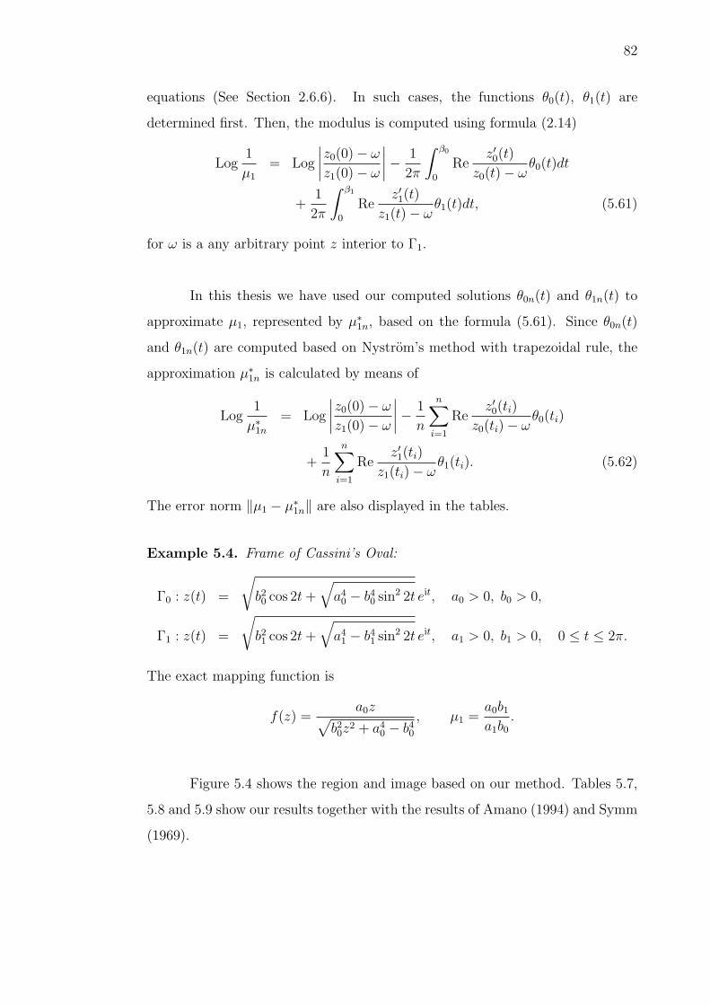
82
equations (See Section 2.6.6). In such cases, the functions θ0(t), θ1(t) are
determined first. Then, the modulus is computed using formula (2.14)
Log1
µ1
= Log
∣∣∣∣z0(0)− ω
z1(0)− ω
∣∣∣∣−1
2π
∫ β0
0
Rez′0(t)
z0(t)− ωθ0(t)dt
+1
2π
∫ β1
0
Rez′1(t)
z1(t)− ωθ1(t)dt, (5.61)
for ω is a any arbitrary point z interior to Γ1.
In this thesis we have used our computed solutions θ0n(t) and θ1n(t) to
approximate µ1, represented by µ∗1n, based on the formula (5.61). Since θ0n(t)
and θ1n(t) are computed based on Nystrom’s method with trapezoidal rule, the
approximation µ∗1n is calculated by means of
Log1
µ∗1n
= Log
∣∣∣∣z0(0)− ω
z1(0)− ω
∣∣∣∣−1
n
n∑i=1
Rez′0(ti)
z0(ti)− ωθ0(ti)
+1
n
n∑i=1
Rez′1(ti)
z1(ti)− ωθ1(ti). (5.62)
The error norm ‖µ1 − µ∗1n‖ are also displayed in the tables.
Example 5.4. Frame of Cassini’s Oval:
Γ0 : z(t) =
√b20 cos 2t +
√a4
0 − b40 sin2 2t eit, a0 > 0, b0 > 0,
Γ1 : z(t) =
√b21 cos 2t +
√a4
1 − b41 sin2 2t eit, a1 > 0, b1 > 0, 0 ≤ t ≤ 2π.
The exact mapping function is
f(z) =a0z√
b20z
2 + a40 − b4
0
, µ1 =a0b1
a1b0
.
Figure 5.4 shows the region and image based on our method. Tables 5.7,
5.8 and 5.9 show our results together with the results of Amano (1994) and Symm
(1969).

83
-10 -5 5 10
-4
-2
2
4
-1 -0.5 0.5 1
-1
-0.5
0.5
1
Figure 5.4: Frame of Cassini’s Oval : a rectangular grid in Ω with grid size 0.25
and its image with a0 = 2√
14, a1 = 2, b0 = 7, and b1 = 1.
Table 5.7: Error Norm (Frame of Cassini’s oval) using our method
N minimal S(x) ‖θ0(t)− θ0n(t)‖∞ ‖θ1(t)− θ1n(t)‖∞16 3.2(−28) 6.3(−03) 1.9(−03)
32 3.1(−28) 6.0(−05) 1.6(−05)
64 7.2(−30) 3.2(−08) 1.2(−08)
128 2.3(−28) 1.9(−08) 7.1(−09)
N ‖µ1 − µ1n‖∞ ‖µ1 − µ∗1n‖∞16 1.5(−03) 3.7(−03)
32 1.3(−05) 2.0(−03)
64 1.8(−09) 5.4(−04)
128 0 1.3(−04)
Table 5.8: Error Norm (Interior of Frame of Cassini’s oval) using our method
N ‖fk(ζ)− f(ζ)‖∞32 9.3(−05)
64 3.8(−08)
128 1.1(−08)

84
Table 5.9: Error Norm (Frame of Cassini’s oval) using Amano’s method and
Symm’s method
Amano’s Method Symm’s Method
N EM EA N EM
16 9.1(−03) 9.7(−03) 64 1.94(−02)
32 3.4(−04) 3.8(−04) 128 3.00(−03)
64 6.9(−07) 5.0(−08) 256 7.00(−04)
128 7.7(−11) 7.7(−11)
Example 5.5. Elliptic Frame:
Γ0 : z(t) = a0 cos t + i b0 sin t, a0 > 0, b0 > 0,
Γ1 : z(t) = a1 cos t + i b1 sin t, a1 > 0, b1 > 0, 0 ≤ t ≤ 2π.
The exact mapping function is
f(z) =z +
√z2 − (a2
0 − b20)
a0 + b0
, µ1 =a1 + b1
a0 + b0
.
Figure 5.5 shows the region and image based on our method. Tables 5.10,
5.11 and 5.12 show our results together with the results of Amano (1994) and
Symm (1969).
-6 -4 -2 2 4 6
-4
-2
2
4
-1 -0.5 0.5 1
-1
-0.5
0.5
1
Figure 5.5: Elliptic Frame : a rectangular grid in Ω with grid size 0.25 and its
image with a0 = 7, a1 = 5, b0 = 5 and b1 = 1.

85
Table 5.10: Error Norm (Elliptic Frame) using our method
N minimal S(x) ‖θ0(t)− θ0n(t)‖∞ ‖θ1(t)− θ1n(t)‖∞16 5.6(−31) 2.3(−03) 6.6(−03)
32 2.8(−19) 3.5(−06) 9.9(−06)
64 3.2(−29) 1.9(−08) 1.7(−08)
128 4.9(−30) 7.6(−09) 6.7(−09)
N ‖µ1 − µ1n‖∞ ‖µ1 − µ∗1n‖∞16 2.0(−03) 9.4(−03)
32 3.0(−06) 1.1(−03)
64 7.0(−12) 1.9(−04)
128 5.6(−17) 4.7(−05)
Table 5.11: Error Norm (Interior of Elliptic Frame) using our method
N ‖fk(ζ)− f(ζ)‖∞32 1.2(−04)
64 3.1(−08)
128 3.3(−09)
Table 5.12: Error norm (Elliptic frame) using Amano’s method and Symm’s
method
Amano’s Method Symm’s Method
N EM EA N EM
16 2.8(−02) 3.8(−03) 64 2.52(−02)
32 3.2(−03) 7.0(−04) 128 3.90(−03)
64 8.4(−05) 2.7(−05) 256 6.00(−04)
128 1.2(−07) 1.8(−07)

86
Example 5.6. Frame of Limacon:
Γ0 : z(t) = a0 cos t + b0 cos 2t + i(a0 sin t + b0 sin 2t), a0 > 0, b0 > 0,
Γ1 : z(t) = a1 cos t + b1 cos 2t + i(a1 sin t + b1 sin 2t), a1 > 0, b1 > 0.
The exact mapping function is
f(z) =
√a2
0 + 4b0z − a0
2b0
, µ1 =a1
a0
.
Figure 5.6 shows the region and image based on our method. Table 5.13,
5.14, and 5.15 show our results together with the result of Symm (1969).
-5 5 10
-10
-5
5
10
-1 -0.5 0.5 1
-1
-0.5
0.5
1
Figure 5.6: Frame of Limacons : a rectangular grid in Ω with grid size 0.4 and
its image with a0 = 10, a1 = 5, b0 = 3 and b1 = b0/4.

87
Table 5.13: Error Norm (Frame of Limacon) using our method
N minimal S(x) ‖θ0(t)− θ0n(t)‖∞ ‖θ1(t)− θ1n(t)‖∞8 1.1(−12) 7.4(−04) 4.8(−04)
16 1.3(−24) 4.2(−06) 1.5(−06)
32 7.5(−30) 7.3(−11) 2.5(−11)
64 6.8(−29) 8.9(−16) 8.9(−16)
N ‖µ1 − µ1n‖∞ ‖µ1 − µ∗1n‖∞8 4.1(−03) 1.7(−03)
16 1.5(−05) 4.1(−04)
32 2.4(−10) 1.0(−04)
64 0 2.6(−05)
Table 5.14: Error Norm (Interior of Frame of Limacon) using our method
N ‖fk(ζ)− f(ζ)‖∞32 1.5(−10)
64 3.4(−14)
Table 5.15: Error Norm (Frame of Limacon) using Symm’s method
N 64 128 256
EM 6.3(−03) 1.0(−03) 2.0(−04)
Example 5.7. Circular Frame:
Γ0 : z(t) = eit,
Γ1 : z(t) = c + ρeit, 0 ≤ t ≤ 2π.

88
The exact mapping function is
f(z) =z − λ
λz − 1, λ =
2c
1 + (c2 − ρ2) +√
(1− (c− ρ)2)(1− (c + ρ)2),
µ1 =2ρ
1− (c2 − ρ2) +√
(1− (c− ρ)2)(1− (c + ρ)2).
Figure 5.7 shows the region and image based on our method. Tables 5.16
and 5.17 show the results.
-1 -0.5 0.5 1
-1
-0.5
0.5
1
-1 -0.5 0.5 1
-1
-0.5
0.5
1
Figure 5.7: Circular Frame : a rectangular grid in Ω with grid size 0.05 and its
image with c = 0.3 and ρ = 0.1.
Table 5.16: Error Norm (Circular Frame) using our method
N minimal S(x) ‖θ0(t)− θ0n(t)‖∞ ‖θ1(t)− θ1n(t)‖∞4 1.6(−07) 5.1(−02) 1.1(−01)
8 2.4(−14) 8.7(−04) 1.7(−04)
16 8.7(−29) 1.3(−07) 2.5(−08)
32 1.6(−30) 1.3(−15) 8.9(−16)
N ‖µ1 − µ1n‖∞ ‖µ1 − µ∗1n‖∞4 2.6(−03) 1.6(−02)
8 3.7(−05) 3.7(−03)
16 4.7(−09) 8.8(−04)
32 4.2(−17) 2.2(−04)

89
Table 5.17: Error Norm (Interior of Circular Frame) using our method
N ‖fk(ζ)− f(ζ)‖∞16 4.6(−08)
32 2.7(−12)
64 1.6(−15)
Example 5.8. Ellipse/Ellipse:
Γ0 : z(t) = 2 cos t + i sin t,
Γ1 : z(t) = cos t + i 0.5 sin t, 0 ≤ t ≤ 2π.
We have adopted this example problem from Ellacott (1979) with µE =
0.5650 for comparison. See Table 5.18 for radius comparisons. Figure 5.8 shows
the region and its image based on our method.
-2 -1 1 2
-1
-0.5
0.5
1
-1 -0.5 0.5 1
-1
-0.5
0.5
1
Figure 5.8: Ellipse/Ellipse : a rectangular grid in Ω with grid size 0.25 and its
image.

90
Table 5.18: The radius comparison for ellipse/ellipse
minimal Value of Radius Comparison
N S(x) µ µ− µE
8 2.6(−25) 0.598436 3.3(−02)
16 5.1(−31) 0.5648148 1.9(−04)
32 3.0(−30) 0.5645690618 4.3(−04)
64 9.3(−30) 0.564569038602491 4.3(−04)
Example 5.9. Ellipse/Circle:
Γ0 : z(t) = 2 cos t + i sin t,
Γ1 : z(t) = 0.5 (cos t + i sin t), 0 ≤ t ≤ 2π.
We have adopted this example problem from Ellacott (1979) with µE =
0.4141 for comparison. See Table 5.19 for radius comparisons. Figure 5.9 shows
the region and its image based on our method.
-2 -1 1 2
-1
-0.5
0.5
1
-1 -0.5 0.5 1
-1
-0.5
0.5
1
Figure 5.9: Ellipse/circle : a rectangular grid in Ω with grid size 0.25 and its
image.
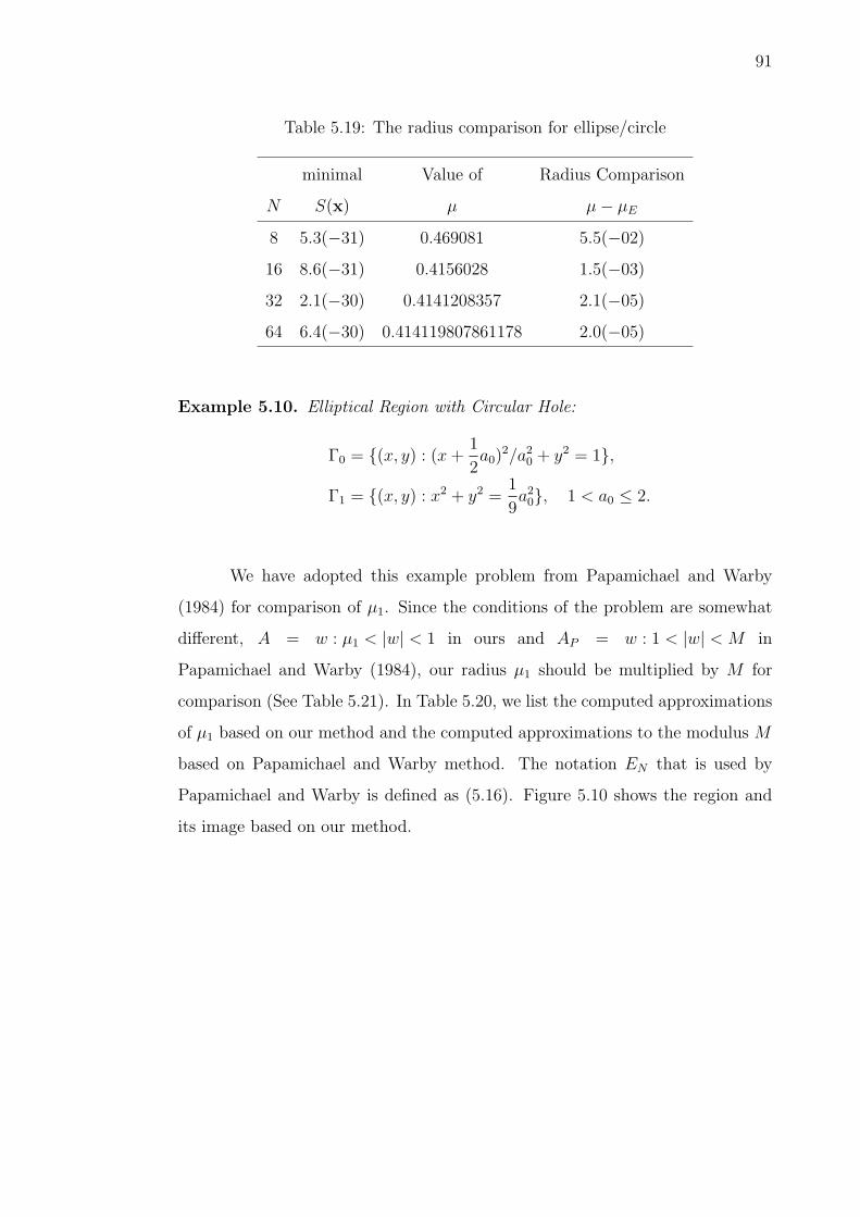
91
Table 5.19: The radius comparison for ellipse/circle
minimal Value of Radius Comparison
N S(x) µ µ− µE
8 5.3(−31) 0.469081 5.5(−02)
16 8.6(−31) 0.4156028 1.5(−03)
32 2.1(−30) 0.4141208357 2.1(−05)
64 6.4(−30) 0.414119807861178 2.0(−05)
Example 5.10. Elliptical Region with Circular Hole:
Γ0 = (x, y) : (x +1
2a0)
2/a20 + y2 = 1,
Γ1 = (x, y) : x2 + y2 =1
9a2
0, 1 < a0 ≤ 2.
We have adopted this example problem from Papamichael and Warby
(1984) for comparison of µ1. Since the conditions of the problem are somewhat
different, A = w : µ1 < |w| < 1 in ours and AP = w : 1 < |w| < M in
Papamichael and Warby (1984), our radius µ1 should be multiplied by M for
comparison (See Table 5.21). In Table 5.20, we list the computed approximations
of µ1 based on our method and the computed approximations to the modulus M
based on Papamichael and Warby method. The notation EN that is used by
Papamichael and Warby is defined as (5.16). Figure 5.10 shows the region and
its image based on our method.

92
-3 -2 -1 1
-1
-0.5
0.5
1
-1 -0.5 0.5 1
-1
-0.5
0.5
1
Figure 5.10: Elliptical region with circular hole : a rectangular grid in Ω with
grid size 0.05 and its image with a0 = 2.0.
Table 5.20: The computed approximations of µ and M for elliptical region with
circular hole
Our Method Papamichael and Warby Method
a0 µ M 1/M
1.04 0.4803797010444083 2.081686628 0.4803797010315426
1.08 0.4869154853494394 2.053744500 0.4869154853488348
1.20 0.5080480086200779 1.968317921 0.5080480085716803
1.40 0.5480734581257743 1.824572938 0.5480734582724585
1.60 0.5938360511745342 1.683966719 0.5938359640467455
1.80 0.6455396040618699 1.549091634 0.6455396040180280
2.00 0.7043817963288784 1.419684616 0.7043817963017217
5.4 Conformal Mapping of Triply Connected Regions onto an
Annulus with a Circular Slit Via the Neumann Kernel
5.4.1 A System of Integral Equations
Suppose Ω is a triply connected region bounded by Γ0, Γ1 and Γ2 (see
Figure 4.3 with M = 2). For the special case where Ω is a triply connected
regions being mapped onto an annulus with a concentric circular slit, the single
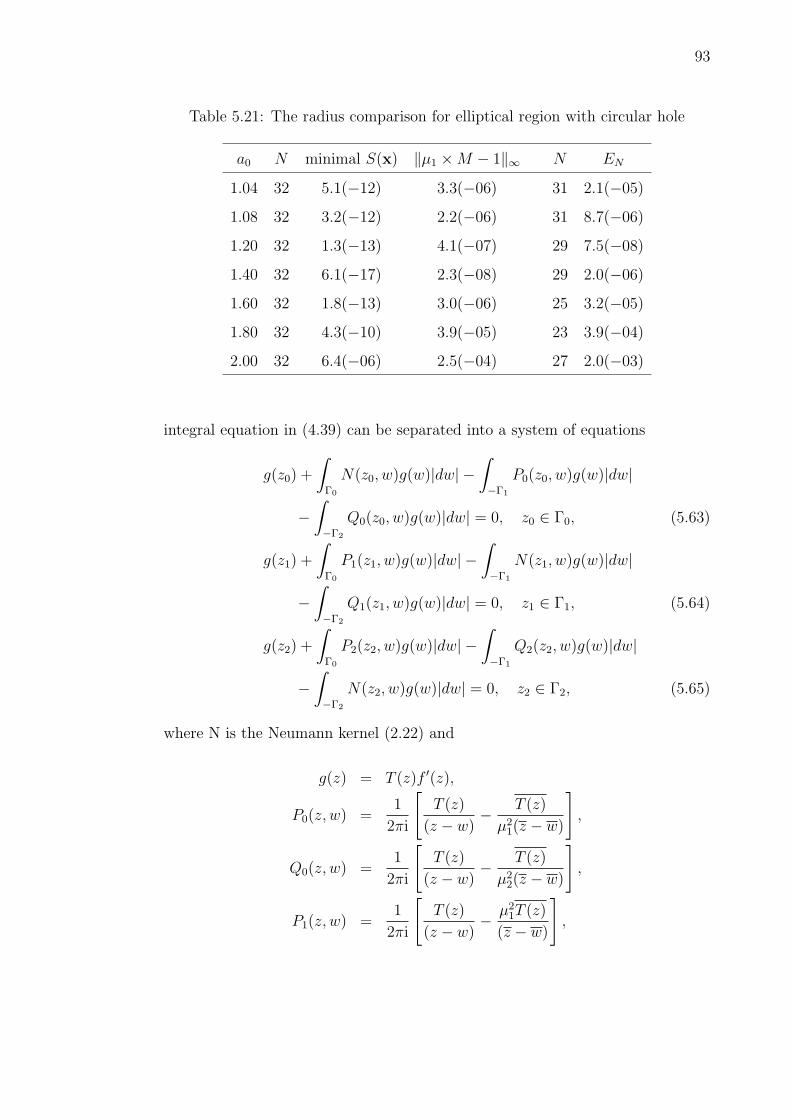
93
Table 5.21: The radius comparison for elliptical region with circular hole
a0 N minimal S(x) ‖µ1 ×M − 1‖∞ N EN
1.04 32 5.1(−12) 3.3(−06) 31 2.1(−05)
1.08 32 3.2(−12) 2.2(−06) 31 8.7(−06)
1.20 32 1.3(−13) 4.1(−07) 29 7.5(−08)
1.40 32 6.1(−17) 2.3(−08) 29 2.0(−06)
1.60 32 1.8(−13) 3.0(−06) 25 3.2(−05)
1.80 32 4.3(−10) 3.9(−05) 23 3.9(−04)
2.00 32 6.4(−06) 2.5(−04) 27 2.0(−03)
integral equation in (4.39) can be separated into a system of equations
g(z0) +
∫
Γ0
N(z0, w)g(w)|dw| −∫
−Γ1
P0(z0, w)g(w)|dw|
−∫
−Γ2
Q0(z0, w)g(w)|dw| = 0, z0 ∈ Γ0, (5.63)
g(z1) +
∫
Γ0
P1(z1, w)g(w)|dw| −∫
−Γ1
N(z1, w)g(w)|dw|
−∫
−Γ2
Q1(z1, w)g(w)|dw| = 0, z1 ∈ Γ1, (5.64)
g(z2) +
∫
Γ0
P2(z2, w)g(w)|dw| −∫
−Γ1
Q2(z2, w)g(w)|dw|
−∫
−Γ2
N(z2, w)g(w)|dw| = 0, z2 ∈ Γ2, (5.65)
where N is the Neumann kernel (2.22) and
g(z) = T (z)f ′(z),
P0(z, w) =1
2πi
[T (z)
(z − w)− T (z)
µ21(z − w)
],
Q0(z, w) =1
2πi
[T (z)
(z − w)− T (z)
µ22(z − w)
],
P1(z, w) =1
2πi
[T (z)
(z − w)− µ2
1T (z)
(z − w)
],

94
Q1(z, w) =1
2πi
[T (z)
(z − w)− µ2
1
µ22
T (z)
(z − w)
],
P2(z, w) =1
2πi
[T (z)
(z − w)− µ2
2T (z)
(z − w)
],
Q2(z, w) =1
2πi
[T (z)
(z − w)− µ2
2
µ21
T (z)
(z − w)
].
As in the doubly connected case, several additional conditions are required
to help achieve uniqueness. The single-valuedness requirement on the mapping
function f(z) implies
∫
−Γ1
g(w)|dw| = 0, (5.66)
∫
−Γ2
g(w)|dw| = 0. (5.67)
The set of equations (5.63) to (5.67) does not guarantee a unique solution.
The conditions (5.21), (5.22), (5.25) and (5.26) are also valid for the triply
connected case under consideration. If the triply connected region is symmetric
with respect to the axes, we can also impose the conditions
Re [g(z1(0))] = 0, (5.68)
Re [g(z2(0))] = 0. (5.69)
Thus the system of integral equations comprising of (5.63), (5.64), (5.65),
(5.66), (5.67) with the conditions (5.21), (5.22), (5.25), (5.26), (5.68) and (5.69)
has a unique solution.
5.4.2 Numerical Implementation
In this section we describe a numerical method for computing the mapping
function f(z), µ1 and µ2 for the case of a triply connected regions. Suppose Γ0,

95
Γ1 and Γ2 be given in parametric representations as follows:
Γ0 : z = z0(t), 0 ≤ t ≤ β0,
Γ1 : z = z1(t), 0 ≤ t ≤ β1,
Γ2 : z = z2(t), 0 ≤ t ≤ β2.
Then the system of integral equations (5.63), (5.64), (5.65), (5.66), (5.67), (5.25)
and (5.26) become
g(z0(t)) +
∫ β0
0
N(z0(t), z0(s))g(z0(s))|z′0(s)|ds
−∫ β1
0
P0(z0(t), z1(s))g(z1(s))|z′1(s)|ds
−∫ β2
0
Q0(z0(t), z2(s))g(z2(s))|z′2(s)|ds = 0, z0(t) ∈ Γ0, (5.70)
g(z1(t)) +
∫ β0
0
P1(z1(t), z0(s))g(z0(s))|z′0(s)|ds
−∫ β1
0
N(z1(t), z1(s))g(z1(s))|z′1(s)|ds
−∫ β2
0
Q1(z1(t), z2(s))g(z2(s))|z′2(s)|ds = 0, z1(t) ∈ Γ1, (5.71)
g(z2(t)) +
∫ β0
0
P2(z2(t), z0(s))g(z0(s))|z′0(s)|ds
−∫ β1
0
Q2(z2(t)), z1(s))g(z1(s))|z′1(s)|ds
−∫ β2
0
N(z2(t), z2(s))g(z2(s))|z′2(s)|ds = 0, z2(t) ∈ Γ2, (5.72)
∫ β1
0
g(z1(s))|z′1(s)|ds = 0, (5.73)
∫ β2
0
g(z2(s))|z′2(s)|ds = 0, (5.74)
∫ β0
0
|g(z0(s))z′0(s)|ds = 2π, (5.75)
∫ β1
0
|g(z1(s))z′1(s)|ds = 2πµ1. (5.76)

96
Multiply (5.70), (5.71) and (5.72) by |z′0(t)|, |z′1(t)| and |z′2(t)| respectively gives
|z′0(t)|g(z0(t)) +
∫ β0
0
|z′0(t)|N(z0(t), z0(s))g(z0(s))|z′0(s)|ds
−∫ β1
0
|z′0(t)|P0(z0(t), z1(s))g(z1(s))|z′1(s)|ds
−∫ β2
0
|z′0(t)|Q0(z0(t), z2(s))g(z2(s))|z′2(s)|ds = 0, z0(t) ∈ Γ0,(5.77)
|z′1(t)|g(z1(t)) +
∫ β0
0
|z′1(t)|P1(z1(t), z0(s))g(z0(s))|z′0(s)|ds
−∫ β1
0
|z′1(t)|N(z1(t), z1(s))g(z1(s))|z′1(s)|ds
−∫ β2
0
|z′1(t)|Q1(z1(t), z2(s))g(z2(s))|z′2(s)|ds = 0, z1(t) ∈ Γ1.(5.78)
|z′2(t)|g(z2(t)) +
∫ β0
0
|z′2(t)|P2(z2(t), z0(s))g(z0(s))|z′0(s)|ds
−∫ β1
0
|z′2(t)|Q2(z2(t)), z1(s))g(z1(s))|z′1(s)|ds
−∫ β2
0
|z′2(t)|N(z2(t), z2(s))g(z2(s))|z′2(s)|ds = 0, z2(t) ∈ Γ2. (5.79)
We next define
φ0(t) = |z′0(t)|g(z0(t)),
φ1(t) = |z′1(t)|g(z1(t)),
φ2(t) = |z′2(t)|g(z2(t)),
K00(t0, s0) = |z′0(t)|N(z0(t), z0(s)),
K01(t0, s1) = |z′0(t)|P0(z0(t), z1(s)),
K02(t0, s2) = |z′0(t)|Q0(z0(t), z2(s)),
K10(t1, s0) = |z′1(t)|P1(z1(t), z0(s)),
K11(t1, s1) = |z′1(t)|N(z1(t), z1(s)),
K12(t1, s2) = |z′1(t)|Q1(z1(t), z2(s)),
K20(t2, s0) = |z′2(t)|P2(z2(t), z0(s)),
K21(t2, s1) = |z′2(t)|Q2(z2(t), z1(s)),
K22(t2, s2) = |z′2(t)|N(z2(t), z2(s)).

97
Thus equations (5.77), (5.78), (5.79), (5.73), (5.74), (5.75) and (5.76) can be
briefly written as
φ0(t) +
∫ β0
0
K00(t0, s0)φ0(s)ds−∫ β1
0
K01(t0, s1)φ1(s)ds
−∫ β2
0
K02(t0, s2)φ2(s)ds = 0, z0(t) ∈ Γ0, (5.80)
φ1(t) +
∫ β0
0
K10(t1, s0)φ0(s)ds−∫ β1
0
K11(t1, s1)φ1(s)ds
−∫ β2
0
K12(t1, s2)φ2(s)ds = 0, z1(t) ∈ Γ1, (5.81)
φ2(t) +
∫ β0
0
K20(t2, s0)φ0(s)ds−∫ β1
0
K21(t2, s1)φ1(s)ds
−∫ β2
0
K22(t2, s2)φ2(s)ds = 0, z2(t) ∈ Γ2, (5.82)
∫ β1
0
φ1(s)ds = 0, (5.83)
∫ β2
0
φ2(s)ds = 0, (5.84)
∫ β0
0
|φ0(s)|ds = 2π, (5.85)
∫ β1
0
|φ1(s)|ds = 2πµ1. (5.86)
We choose β0 = β1 = β2 = 2π and n equidistant collocation points ti =
(i− 1)β0/n, 1 ≤ i ≤ n on Γ0, m equidistant collocation points ti = (i− 1)β1/m,
1 ≤ i ≤ m, on Γ1 and l equidistant collocation points ti = (i− 1)β2/l, 1 ≤ i ≤ l,
on Γ2. Applying the Nystrom’s method with trapezoidal rule to discretize (5.80)
to (5.86), we obtain
φ0(ti) +β0
n
n∑j=1
K00(ti, tj)φ0(tj)− β1
m
m∑
j=1
K01(ti, tj)φ1(tj)
− β2
l
l∑
j=1
K02(ti, tj)φ2(tj) = 0, (5.87)
φ1(ti) +β0
n
n∑j=1
K10(ti, tj)φ0(tj)− β1
m
m∑
j=1
K11(ti, tj)φ1(tj)
− β2
l
l∑
j=1
K12(ti, tj)φ2(tj) = 0, (5.88)

98
φ2(ti) +β0
n
n∑j=1
K20(ti, tj)φ0(tj)− β1
m
m∑
j=1
K21(ti, tj)φ1(tj)
− β2
l
l∑
j=1
K22(ti, tj)φ2(tj) = 0, (5.89)
m∑
j=1
φ1(tj) = 0, (5.90)
l∑
j=1
φ2(tj) = 0, (5.91)
n∑j=1
|φ0(tj)| = n, (5.92)
m∑
j=1
|φ1(tj)| = mµ1. (5.93)
Equations (5.87) to (5.93) lead to a system of (n + m + l + 4) non-linear
complex equations in n unknowns φ0(ti), m unknowns φ1(ti), l unknowns φ2(ti),
µ1 and µ2, as well as the unknown parameters µ1 and µ2. By defining the matrix
x0i = φ0(ti), x1i = φ1(ti), x2i = φ2(ti),
Bij =β0
nK00(ti, tj), Cij =
β1
mK01(ti, tj), Dij =
β2
lK02(ti, tj),
Eij =β0
nK10(ti, tj), Fij =
β1
mK11(ti, tj), Gij =
β2
lK12(ti, tj),
Hij =β0
nK20(ti, tj), Jij =
β1
mK21(ti, tj), Lij =
β2
lK22(ti, tj),
the system of equations (5.87), (5.88) and (5.89) can be written as n + m + l by
n + m + l system of non-linear equations
[Inn + Bnn]x0n − Cnmx1m −Dnlx2l = 0, (5.94)
Emnx0n + [Imm − Fmm]x1m −Gmlx2l = 0, (5.95)
Hlnx0n − Jlmx1m + [Ill − Lll]x2l = 0. (5.96)

99
The result in matrix form for the system of equations (5.94), (5.95) and (5.96) is
Inn + Bnn · · · −Cnm · · · −Dnl
.... . .
.... . .
...
Emn · · · Imm − Fmm · · · Gml
.... . .
.... . .
...
Hln · · · −Jlm · · · Ill − Lll
x0n
...
x1m
...
x2l
=
00n
...
01m
...
02l
. (5.97)
Defining
A =
Inn + Bnn · · · −Cnm · · · −Dnm
.... . .
.... . .
...
Emn · · · Imm − Fmm · · · −Gmm
.... . .
.... . .
...
Hln · · · −Jlm · · · Ill − Lll
,
x=
x0n
...
x1m
...
x2l
, and 0 =
00n
...
01m
...
02l
,
the (n+m+ l)× (n+m+ l) system can be written briefly as Ax = 0. Separating
A and x in terms of the real and imaginary parts, the system can be written as
ReARex− ImA Imx + i( ImARex + ReA Imx) = 0 + 0i. (5.98)
The single (n + m + l)× (n + m + l) complex system (5.98) can also be written
as 2(n + m + l)× 2(n + m + l) system matrix
Re A · · · Im A...
. . ....
Im A · · · Re A
Re x...
Im x
=
0...
0
. (5.99)

100
Note however that the 2(n+m+ l)×2(n+m+ l) matrix in (5.99) contains
the unknown parameters µ1 and µ2. Since φ = Re φ + i Im φ, equations (5.90),
(5.91), (5.92), (5.93), (5.21), (5.22), (5.68) and (5.69) become
m∑
j=1
(Re x1j + i Im x1j) = 0, (5.100)
l∑
j=1
(Re x2j + i Im x2j) = 0, (5.101)
n∑j=1
√(Re x0j)2 + (Im x0j)2 = n, (5.102)
m∑
j=1
√(Re x1j)
2 + (Im x1j)2 = mµ1, (5.103)
Re x01 = 0, (5.104)
Im [x01/√
(Re x01)2 + (Im x01)2] = 1, (5.105)
Re x11 = 0, (5.106)
Re x21 = 0, (5.107)
Thus a unique solution can be obtained from the system of equations (5.99)
to (5.107). This system is an over-determined system of nonlinear equations
involving 2(n + m + l) + 8 equations in 2(n + m + l) + 2 unknowns. We use a
modification of the Gauss-Newton called the Lavenberg-Marquardt algorithm to
solve this nonlinear least square problem. The Lavenberg-Marquardt algorithm
which is stated in (5.56), i.e.
xk+1 = xk −H(xk)f(xk), λk ≥ 0,
where H(xk) = ((Jf (xk))T Jf (xk)+λkI)−1(Jf (xk))
T and Jf (x). Here, x stands for
the 2(n + m + l) + 2 vector (Re x01, Re x02, ..., Re x0n, Re x11, Re x12, ..., Re x1m,
Re x21, Re x22, ..., Re x2l, Im x01, Im x02, ..., Im x0n, Im x11, Im x12, ..., Im x1m,
Im x21, Im x22, ..., Im x2l, µ1, µ2), and f = (f1, f2, ..., f2(n+m+l)+8).
Our strategy for getting the initial estimation x0 is based on (4.27) and

101
(4.28) where upon differentiating, we obtain
φ0(t) = f ′(z0(t))z′0(t) = iθ′0(t)e
iθ0(t),
φ1(t) = f ′(z1(t))z′1(t) = µ1iθ
′1(t)e
iθ1(t),
φ2(t) = f ′(z2(t))z′2(t) = µ2iθ
′2(t)e
iθ2(t).
For initial estimation, we assume θ0(t) = θ1(t) = θ2(t) = t which implies
θ′0(t) = θ′1(t) = θ′2(t) = 1 and choose µ1 = µ2 = 0.5 as our initial guess of the
inner radii. In our experiments, we have chosen the number of collocation points
on Γ0, Γ1 and Γ2 being equal, N , i.e., n = m = l. After solving this system
of equation for the unknown functions φ0(t) = |z′0(t)|T (z0(t))f′(z0(t)), φ1(t) =
|z′1(t)|T (z1(t))f′(z1(t)), φ2(t) = |z′2(t)|T (z2(t))f
′(z2(t)), µ1 and µ2, the boundary
correspondence functions θ0(t), θ1(t) and θ2(t) are then computed approximately
by the formulas
θ0(t) = Arg f(z0(t)) ≈ Arg (−iφ0(t)),
θ1(t) = Arg f(z1(t)) ≈ Arg (−iφ1(t)),
θ2(t) = Arg f(z2(t)) ≈ Arg (±iφ2(t)).
5.4.3 Interior of Triply Connected Region
Section 5.4.2 deal with conformal mapping on the boundary of triply
connected regions. In this section, we describe a numerical procedure for
computing the mapping of interior points. Once the boundary values of the
mapping function f are known, the values of the mapping function for triply
connected regions may be calculated by quadrature at any interior points of its
domain of definition through Cauchy’s integral formula (see Theorem 5.1).

102
Let f be analytic on the boundaries Γ = Γ0 ∪ Γ1 ∪ Γ2 and the region Ω
bounded by Γ0, Γ1 and Γ2. If ζ is any point on Ω, then
f(ζ) =1
2πi
∫
Γ
f(z)
z − ζdz
=1
2πi
∫
Γ0
f(z)
z − ζdz − 1
2πi
∫
−Γ1
f(z)
z − ζdz − 1
2πi
∫
−Γ2
f(z)
z − ζdz.(5.108)
The Cauchy’s integral formula (5.108) can be also written in the parametrized
form, i.e.
f(ζ) =1
2πi
∫ β0
0
f(z0(t))z′0(t)
z0(t)− ζdt− 1
2πi
∫ β1
0
f(z1(t))z′1(t)
z1(t)− ζdt
− 1
2πi
∫ β2
0
f(z2(t))z′2(t)
z2(t)− ζdt. (5.109)
By means of (4.27) and (4.28), the Cauchy’s integral formula (5.108) can then be
written in the form
f(ζ) =1
2πi
∫ β0
0
eiθ0(t)z′0(t)z0(t)− ζ
dt− 1
2πi
∫ β1
0
µ1eiθ1(t)z′1(t)
z1(t)− ζdt
− 1
2πi
∫ β2
0
µ2eiθ2(t)z′2(t)
z2(t)− ζdt. (5.110)
For the points which are not close to the boundary, the integrands are
well behaved. However for points near the boundary, the numerical integration is
inaccurate due to the influence of the singularity. This difficulty is overcome
through the introduction of an iterative technique as given in (5.60) (see
Swarztrauber (1972)).
5.4.4 Numerical Results
For numerical experiment, we have used two test regions. We have not
found any exact mapping function documented in the literature. These test
region are chosen base on the example in the Reichel (1986), Okano et al. (2003),

103
Kokkinos et al. (1990) and Ellacott (1979). We have adopted the example
problem from the above literature for comparison. All the computations were
done using MATHEMATICA package (Wolfram, 1991) in single precision (16
digit machine precision).
Example 5.11. Ellipse/two circles:
Let
Γ0 : z0(t) = 2 cos t + i sin t,
Γ1 : z1(t) = 0.5 (cos t + i sin t),
Γ2 : z2(t) = 1.2 + 0.3 (cos t + i sin t), t : 0 ≤ t ≤ 2π.
We have adopted the example problems from Reichel (1986) and Kokkinos
et al. (1990) for comparison of µ1 and µ2 (see Tables 5.22 and 5.23). We obtain
the results µ1 = 0.42588654195460685 and µ2 = 0.810970795718853. Since the
conditions of the problems are somewhat different, µ0 = 1 in ours, µ0 = 1.5 in
Reichel’s and µ0 = 2 in Kokkinos et al., our radii µ1 and µ2 should be multiplied
by 1.5 and 2 respectively. Values of µ1 and µ2 in Reichel are denoted here by
µ1,R and µ2,R respectively. While the values of µ1 and µ2 in Kokkinos et al . are
denoted here by µ1,K and µ2,K respectively. Figure 5.11 shows the region and its
image based on our method.
-2 -1 1 2
-1
-0.5
0.5
1
-1 -0.5 0.5 1
-1
-0.5
0.5
1
Figure 5.11: Ellipse/two circles : a rectangular grid in Ω with grid size 0.05 and
its image.
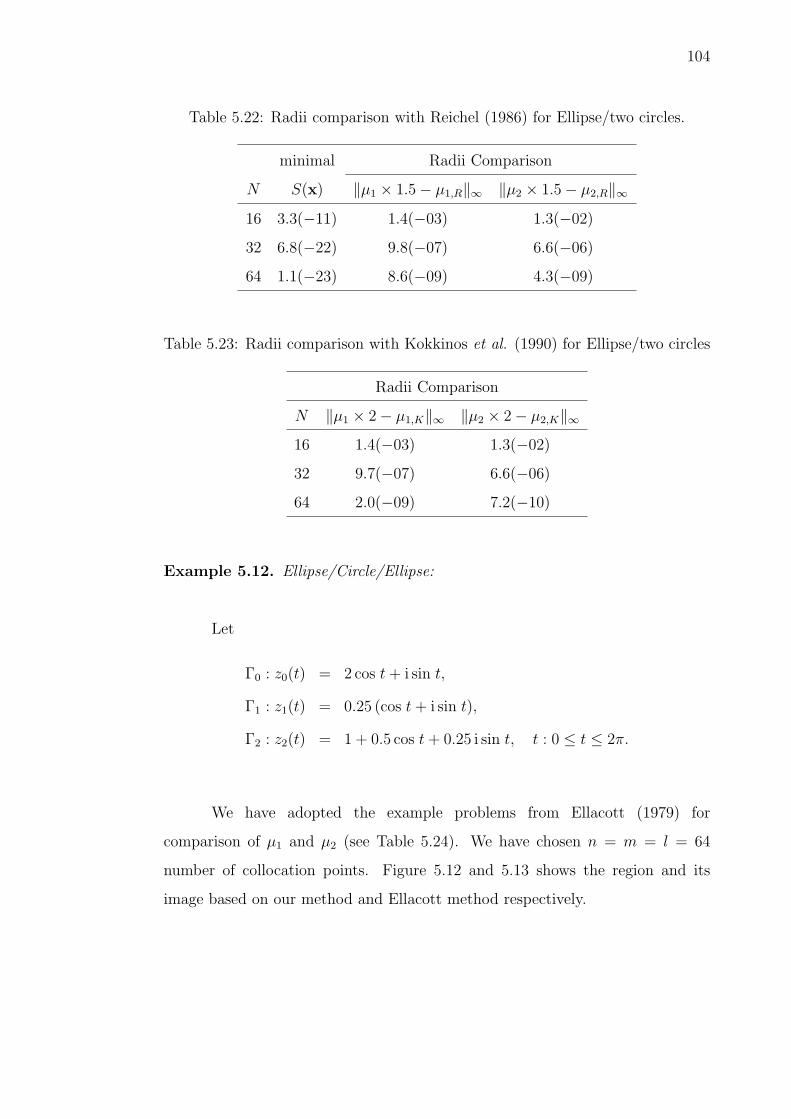
104
Table 5.22: Radii comparison with Reichel (1986) for Ellipse/two circles.
minimal Radii Comparison
N S(x) ‖µ1 × 1.5− µ1,R‖∞ ‖µ2 × 1.5− µ2,R‖∞16 3.3(−11) 1.4(−03) 1.3(−02)
32 6.8(−22) 9.8(−07) 6.6(−06)
64 1.1(−23) 8.6(−09) 4.3(−09)
Table 5.23: Radii comparison with Kokkinos et al. (1990) for Ellipse/two circles
Radii Comparison
N ‖µ1 × 2− µ1,K‖∞ ‖µ2 × 2− µ2,K‖∞16 1.4(−03) 1.3(−02)
32 9.7(−07) 6.6(−06)
64 2.0(−09) 7.2(−10)
Example 5.12. Ellipse/Circle/Ellipse:
Let
Γ0 : z0(t) = 2 cos t + i sin t,
Γ1 : z1(t) = 0.25 (cos t + i sin t),
Γ2 : z2(t) = 1 + 0.5 cos t + 0.25 i sin t, t : 0 ≤ t ≤ 2π.
We have adopted the example problems from Ellacott (1979) for
comparison of µ1 and µ2 (see Table 5.24). We have chosen n = m = l = 64
number of collocation points. Figure 5.12 and 5.13 shows the region and its
image based on our method and Ellacott method respectively.

105
Table 5.24: Radii comparison for Ellipse/two circles
Our Method Ellacott (1979)
Radius Radius ‖µp − µp,E‖∞µ1 = 0.24061238546734354 µ1,E = 0.25 9.4(−03)
µ2 = 0.6859816257842841 µ2,E = 0.68 6.0(−03)
-2 -1 1 2
-1
-0.5
0.5
1
-1 -0.5 0.5 1
-1
-0.5
0.5
1
Figure 5.12: Ellipse/Circle/Ellipse : a rectangular grid in Ω with grid size 0.05
and its image.
Figure 5.13: Conformal mapping of Ellipse/circles/ellipse onto an annulus with
a concentric circular slit base on Ellacott method.

CHAPTER 6
NUMERICAL CONFORMAL MAPPING OF MULTIPLY
CONNECTED REGIONS ONTO A DISK WITH CIRCULAR SLITS
6.1 Introduction
We have shown in Chapter 5 that the proposed method for the
numerical conformal mapping of multiply connected regions onto an annulus
with circular slits via the Kerzman-Stein and the Neumann kernels can produced
approximations of high accuracy. In this chapter, we shall discuss numerical
aspects of conformal mapping of multiply connected regions onto a disk with
circular slits based on the integral equation developed in Chapter 4.
6.2 Conformal Mapping of Doubly Connected Regions onto a Disk
with a Circular Slit Via the Neumann Kernel
6.2.1 A System of Integral Equations
Suppose Ω is a doubly connected region bounded by Γ0 and Γ1 (see Figure
4.4 with M = 1). For the special case where Ω is a doubly connected region being

107
mapped onto a disk with a circular slit, the single integral equation in (4.58) can
be separated into a system of equations
g(z0, a) +
∫
Γ0
N(z0, w)g(w, a)|dw| −∫
−Γ1
P0(z0, w)g(w, a)|dw|
= r2h(a, z0), z0 ∈ Γ0, (6.1)
g(z1, a) +
∫
Γ0
P1(z1, w)g(w, a)|dw| −∫
−Γ1
N(z1, w)g(w, a)|dw|
= µ21r
2h(a, z1), z1 ∈ Γ1, (6.2)
where
g(z, a) = f ′(a)T (z)f ′(z),
h(a, z) = − T (z)
(a− z)2,
P0(z, w) =1
2πi
[T (z)
(z − w)− T (z)
µ21(z − w)
],
P1(z, w) =1
2πi
[T (z)
(z − w)− µ2
1T (z)
(z − w)
],
N(z, w) =
1
2πi
[T (z)
z − w− T (z)
z − w
], if w, z ∈ Γ, w 6= z,
1
2π
Im[z′′(t)z′(t)]|z′(t)|3 , if w = z ∈ Γ.
The kernel N is also known as Neumann kernel.
Note that there are four unknown quantities in the integral equations (6.1)
and (6.2), namely, g(z0, a), g(z1, a), r and µ1. Naturally it is also required that the
unknown mapping function f(z) be single-valued in the problem domain (Henrici,
1986), i.e. ∫
−Γ1
f ′(w)dw = 0, (6.3)
which implies ∫
−Γ1
g(w, a)|dw| = 0. (6.4)
Several conditions can be obtained to help achieve uniqueness. We first
consider equation (4.47). Upon differentiation and taking modulus to both sides
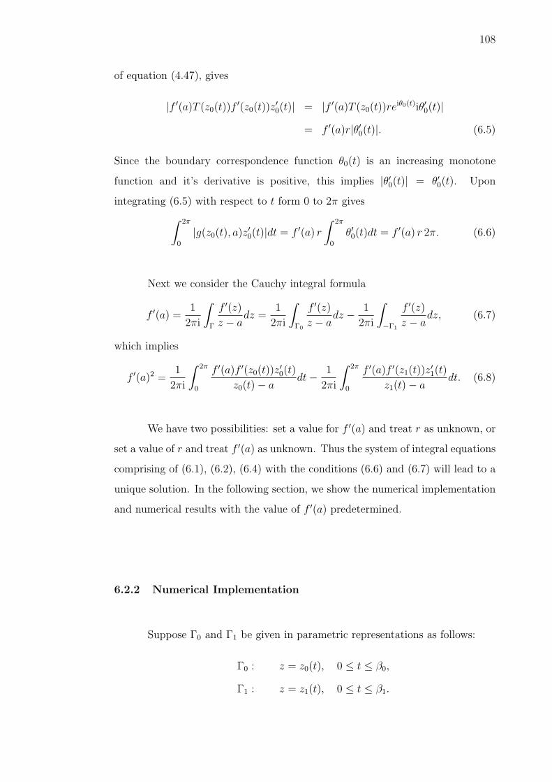
108
of equation (4.47), gives
|f ′(a)T (z0(t))f′(z0(t))z
′0(t)| = |f ′(a)T (z0(t))re
iθ0(t)iθ′0(t)|= f ′(a)r|θ′0(t)|. (6.5)
Since the boundary correspondence function θ0(t) is an increasing monotone
function and it’s derivative is positive, this implies |θ′0(t)| = θ′0(t). Upon
integrating (6.5) with respect to t form 0 to 2π gives
∫ 2π
0
|g(z0(t), a)z′0(t)|dt = f ′(a) r
∫ 2π
0
θ′0(t)dt = f ′(a) r 2π. (6.6)
Next we consider the Cauchy integral formula
f ′(a) =1
2πi
∫
Γ
f ′(z)
z − adz =
1
2πi
∫
Γ0
f ′(z)
z − adz − 1
2πi
∫
−Γ1
f ′(z)
z − adz, (6.7)
which implies
f ′(a)2 =1
2πi
∫ 2π
0
f ′(a)f ′(z0(t))z′0(t)
z0(t)− adt− 1
2πi
∫ 2π
0
f ′(a)f ′(z1(t))z′1(t)
z1(t)− adt. (6.8)
We have two possibilities: set a value for f ′(a) and treat r as unknown, or
set a value of r and treat f ′(a) as unknown. Thus the system of integral equations
comprising of (6.1), (6.2), (6.4) with the conditions (6.6) and (6.7) will lead to a
unique solution. In the following section, we show the numerical implementation
and numerical results with the value of f ′(a) predetermined.
6.2.2 Numerical Implementation
Suppose Γ0 and Γ1 be given in parametric representations as follows:
Γ0 : z = z0(t), 0 ≤ t ≤ β0,
Γ1 : z = z1(t), 0 ≤ t ≤ β1.
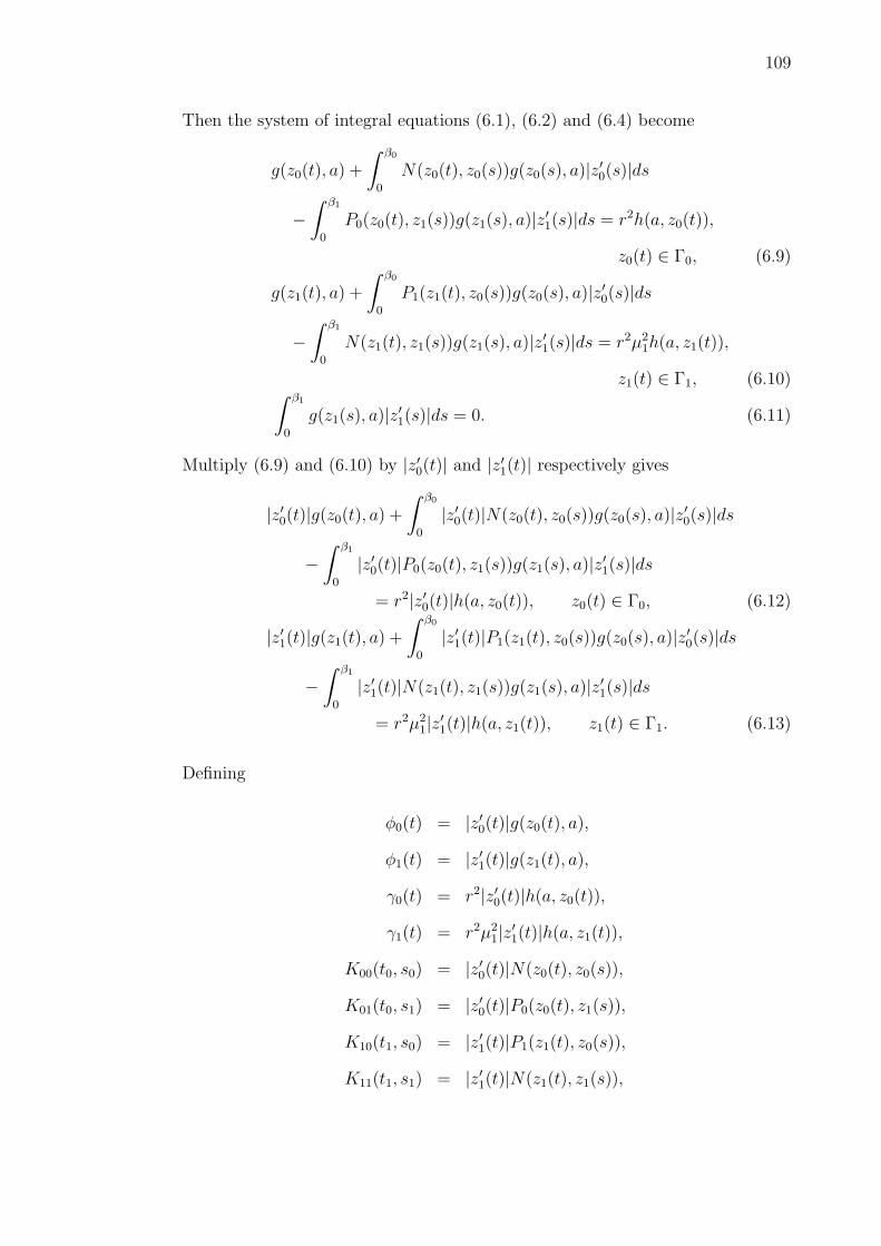
109
Then the system of integral equations (6.1), (6.2) and (6.4) become
g(z0(t), a) +
∫ β0
0
N(z0(t), z0(s))g(z0(s), a)|z′0(s)|ds
−∫ β1
0
P0(z0(t), z1(s))g(z1(s), a)|z′1(s)|ds = r2h(a, z0(t)),
z0(t) ∈ Γ0, (6.9)
g(z1(t), a) +
∫ β0
0
P1(z1(t), z0(s))g(z0(s), a)|z′0(s)|ds
−∫ β1
0
N(z1(t), z1(s))g(z1(s), a)|z′1(s)|ds = r2µ21h(a, z1(t)),
z1(t) ∈ Γ1, (6.10)∫ β1
0
g(z1(s), a)|z′1(s)|ds = 0. (6.11)
Multiply (6.9) and (6.10) by |z′0(t)| and |z′1(t)| respectively gives
|z′0(t)|g(z0(t), a) +
∫ β0
0
|z′0(t)|N(z0(t), z0(s))g(z0(s), a)|z′0(s)|ds
−∫ β1
0
|z′0(t)|P0(z0(t), z1(s))g(z1(s), a)|z′1(s)|ds
= r2|z′0(t)|h(a, z0(t)), z0(t) ∈ Γ0, (6.12)
|z′1(t)|g(z1(t), a) +
∫ β0
0
|z′1(t)|P1(z1(t), z0(s))g(z0(s), a)|z′0(s)|ds
−∫ β1
0
|z′1(t)|N(z1(t), z1(s))g(z1(s), a)|z′1(s)|ds
= r2µ21|z′1(t)|h(a, z1(t)), z1(t) ∈ Γ1. (6.13)
Defining
φ0(t) = |z′0(t)|g(z0(t), a),
φ1(t) = |z′1(t)|g(z1(t), a),
γ0(t) = r2|z′0(t)|h(a, z0(t)),
γ1(t) = r2µ21|z′1(t)|h(a, z1(t)),
K00(t0, s0) = |z′0(t)|N(z0(t), z0(s)),
K01(t0, s1) = |z′0(t)|P0(z0(t), z1(s)),
K10(t1, s0) = |z′1(t)|P1(z1(t), z0(s)),
K11(t1, s1) = |z′1(t)|N(z1(t), z1(s)),

110
the system of equations (6.12), (6.13), (6.11), (6.6) and (6.8) can be briefly written
as
φ0(t) +
∫ β0
0
K00(t0, s0)φ0(s)ds−∫ β1
0
K01(t0, s1)φ1(s)ds = γ0(t), (6.14)
φ1(t) +
∫ β0
0
K10(t1, s0)φ0(s)ds−∫ β1
0
K11(t1, s1)φ1(s)ds = γ1(t), (6.15)
∫ β1
0
φ1(s)ds = 0, (6.16)
∫ β0
0
|φ0(s)|ds = f ′(a)r2π, (6.17)
1
2πi
∫ β0
0
φ0(s)
z0(s)− ads− 1
2πi
∫ β1
0
φ1(s)
z1(s)− ads = f ′(a)2. (6.18)
Since the functions φ, γ, and K in the above systems are β-periodic, a
reliable procedure for solving (6.14) to (6.18) numerically is using the Nystrom’s
method with trapezoidal rule (Atkinson, 1976). We choose β0 = β1 = 2π and n
equidistant collocation points ti = (i−1)β0/n, 1 ≤ i ≤ n on Γ0 and m equidistant
collocation points tı = (ı − 1)β1/m, 1 ≤ ı ≤ m, on Γ1. Applying the Nystrom’s
method with trapezoidal rule to discretize (6.14) to (6.18), we obtain
φ0(ti) +β0
n
n∑j=1
K00(ti, tj)φ0(tj)− β1
m
m∑=1
K01(ti, t)φ1(t) = γ0(ti), (6.19)
φ1(tı) +β0
n
n∑j=1
K10(tı, tj)φ0(tj)− β1
m
m∑=1
K11(tı, t)φ1(t) = γ1(tı), (6.20)
m∑=1
φ1(t) = 0, (6.21)
n∑j=1
|φ0(tj)| = f ′(a)rn, (6.22)
1
ni
n∑j=1
1
z0(tj)− aφ0(tj)− 1
mi
m∑=1
1
z1(t)− aφ1(t) = f ′(a)2. (6.23)
Equations (6.19) to (6.23) lead to a system of (n + m + 3) non-linear
complex equations in n unknowns φ0(ti), m unknowns φ1(tı), f ′(a), r and µ1. By

111
defining the matrices
x0i = φ0(ti),
x1ı = φ1(tı),
γ0i = γ0(ti),
γ1ı = γ1(tı),
Bij =β0
nK00(ti, tj),
Ci =β1
mK01(ti, t),
Eıj =β0
nK10(tı, tj),
Dı =β1
mK11(tı, t),
Fn =1
in
n∑j=1
1
z0(tj)− a,
Gm =1
im
m∑=1
1
z1(t)− a,
the system of equations (6.19), (6.20) and (6.23) can be written as n + m + 1 by
n + m system of equations
[Inn + Bnn]x0n − Cnmx1m = γ0n, (6.24)
Emnx0n + [Imm −Dmm]x1m = γ1m, (6.25)
Fnx0n + Gmx1m = f ′(a)2. (6.26)
Since φ = Re φ + i Im φ, equations (6.21) and (6.22) becomes
m∑=1
(Re x1 + i Im x1) = 0, (6.27)
n∑j=1
√(Re x0j)2 + (Im x0j)2 = f ′(a)rn. (6.28)

112
The result in matrix form for the system of equations (6.24), (6.25) and (6.26) is
Inn + Bnn · · · −Cnm
.... . .
...
Emn · · · Imm −Dmm
.... . .
...
Fn · · · Gm
x0n
...
x1m
=
γ0n
...
γ1m
...
f ′(a)2
. (6.29)
Defining
A =
Inn + Bnn · · · −Cnm
.... . .
...
Emn · · · Imm −Dmm
.... . .
...
Fn · · · Gm
,x=
x0n
...
x1m
and y =
γ0n
...
γ1m
...
f ′(a)2
,
the (n + m + 1)× (n + m) system can be written briefly as Ax = y. Separating
A, x and y in terms of the real and imaginary parts, the system can be written
as
ReARex− ImA Imx + i( ImARex + ReA Imx) = Rey + i Imy. (6.30)
The single (n + m + 1) × (n + m) complex system (6.30) above is equivalent to
the 2(n+m+1)×2(n+m) system matrix involving the real (Re) and imaginary
(Im) of the unknown functions, i.e.,
Re A · · · Im A...
. . ....
Im A · · · Re A
Re x...
Im x
=
Re y...
Im y
. (6.31)
Note that the matrix in (6.31) contains the unknown parameters r and
µ1. The value of f ′(a) is predetermined. The system of equations (6.31), (6.27)
and (6.28) is an over-determined system of non-linear equations involving 2(n +
m + 1) + 2 equations in 2(n + m) + 2 unknowns.

113
We use a modification of the Gauss-Newton called the Lavenberg-
Marquardt with the Fletcher’s algorithm to solve this nonlinear least square
problem. Our nonlinear least square problem consists in finding the vector x
for which the function S : R2(n+m)+4 → R1 defined by the sum of squares
S(x) = fTf =
2(n+m)+4∑i=1
(fi(x))2
is minimal. Here, x stands for the 2(n+m)+2 vector (Re x01, Re x02, ..., Re x0n,
Re x11, Re x12, ..., Re x1m, Im x01, Im x02, ..., Im x0n, Im x11, Im x12, ..., Im x1m,
µ1, r), and f = (f1, f2, ..., f2(n+m+1)+2). The Lavenberg-Marquardt algorithm is an
iterative procedure with starting value denoted as x0. This initial approximation,
which, if at all possible, should be well-informed guess and generate a sequence
of approximations x1, x2, x3, ... base on the formula (5.56) i.e.
xk+1 = xk −H(xk)f(xk), λk ≥ 0,
where H(xk) = ((Jf (xk))TJf (xk) + λkI)−1(Jf (xk))
T.
The strategy for getting the initial estimation is to provide rough estimates
of the slit radius, µ ≈ 0.5, r = 1 and set f ′(a) = 1 for the test region. Then
the non-linear system of equations (6.29) and (6.27) reduces to over-determined
linear system. Writing the over-determined system as Bx = y, we use the least-
squares solutions of Bx = y which are precisely the solutions of BTBx = BTy
(Johnson et al., 1998). The solutions are then taken as initial estimation. These
initial guesses are applied for the lowest number of n and m of our experiments.
In all our experiments, we have chosen the number of collocation points on Γ0
and Γ1 being equal, i.e., n = m. The information from the solution of µ1 and r
of lower n is then exploited as an estimate of µ1 and r for the next 2n number of
collocations points.
The system of equations (6.31) with (6.27) and (6.28) are then solved for
the unknown functions
φ0(t) = |z′0(t)|f ′(a)T (z0(t))f′(z0(t)),

114
φ1(t) = |z′1(t)|f ′(a)T (z1(t))f′(z1(t)),
µ and r. Finally the boundary correspondence functions θ0(t) and θ1(t) are
computed approximately by the formulas
θ0(t) = Arg f(z0(t)) ≈ Arg(−iφ0(t)),
θ1(t) = Arg f(z1(t)) ≈ Arg(±iφ1(t)).
6.2.3 The Interior Mapping
Once the boundary values of the mapping function f are known, the values
of the mapping function may be calculated by quadrature at any interior points
of its domain of definition through Cauchy’s integral formula (see Theorem 5.1).
By using (4.47) and (4.48), the Cauchy’s integral formula (5.57) can then
be written in the form
f(ζ) =1
2πi
∫ β0
0
reiθ0(t)z′0(t)z0(t)− ζ
dt− 1
2πi
∫ β1
0
µ1reiθ1(t)z′1(t)
z1(t)− ζdt, (6.32)
where ζ is any point on Ω.
For the points which are close to the boundary, we use the iterative
technique as given in equation (5.60). In practice the iteration converges rapidly.
Using this technique, we are able to maintain the same accuracy throughout the
region Ω.

115
6.2.4 Numerical Results
For numerical results, we have used five test regions whose exact boundary
correspondence functions are known as given in Section 2.5. The test regions are
annulus, frame of Limacon, elliptic frame, circular frame and frame of Cassini’s
oval. We set f ′(a) = 1 for all test regions. Note that, f(z) maps Ω conformally
onto a disk |w| < r with a circular slit of radius µ1r, where 0 < µ1 < 1. Thus
g(z) = f(z)/r maps Ω onto a disk |w| < 1 with a circular slit of radius µ1. This
implies that f and g have the same values of θ0(t), θ1(t) and µ1. The results for
the sub-norm error between the exact values of θ0(t), θ1(t), µ1, f(ζ) and their
corresponding approximations θ0n(t), θ1n(t), µ1n, fk(ζ) are shown in Tables 6.1
to 6.10. Figures 5.1 to 5.5 shows the regions and corresponding images based
on our method. All the computations are done using MATHEMATICA package
(Wolfram, 1991) in single precision (16 digit machine precision).
Example 6.1. Annulus:
Γ0 : z(t) = cos t + i sin t,
Γ1 : z(t) = r(cos t + i sin t), 0 ≤ t ≤ 2π.
The exact mapping function is
g(z) = −e2σ
θ4
(1
2ilog z +
iπτ
2− iσ; q
)
θ4
(1
2ilog z +
iπτ
2+ iσ; q
) , 0 < σ <πτ
2, µ1 = e−2σ.
For the purpose of numerical comparison, we set r = q = e−πτ (see Section
2.5.1) and since θ4(πτ i/2; q) = 0 (Whittaker and Watson, 1927), this implies
a = e−2σ. We have chosen τ = 0.50, and σ = 0.20. Figure 6.1 shows the region
and image based on our method. See Tables 6.1 and 6.2 for results.

116
-1 -0.5 0.5 1
-1
-0.5
0.5
1
-1 -0.5 0.5 1
-1
-0.5
0.5
1
Figure 6.1: Annulus : a rectangular grid in Ω with grid size 0.05 and its image
with radius µ1 = e−2σ.
Table 6.1: Error Norm (Annulus)
n = m minimal S(x) ‖θ0(t)− θ0n(t)‖∞ ‖θ1(t)− θ1n(t)‖∞ ‖µ1 − µ1n‖∞16 8.4(−15) 1.9(−02) 6.3(−01) 1.7(−02)
32 2.7(−24) 5.0(−05) 8.9(−04) 2.8(−05)
64 3.5(−30) 2.4(−10) 2.3(−09) 8.2(−11)
128 2.4(−30) 8.9(−16) 7.0(−14) 2.2(−16)
Table 6.2: Error Norm (Interior of Annulus)
n = m ‖fk(ζ)− f(ζ)‖∞32 1.8(−04)
64 3.0(−10)
128 1.3(−15)
Example 6.2. Circular Frame:
Γ0 : z(t) = eit,
Γ1 : z(t) = c + ρeit, 0 ≤ t ≤ 2π.

117
The exact mapping function is
g(z) = e2σ
θ4
(1
2ilog f(z) +
iπτ
2− iσ; q
)
θ4
(1
2ilog f(z) +
iπτ
2+ iσ; q
) , 0 < σ <πτ
2, µ1 = e−2σ,
with
f(z) =z − λ
λz − 1, λ =
2c
1 + (c2 − ρ2) +√
(1− (c− ρ)2)(1− (c + ρ)2),
r =2ρ
1− (c2 − ρ2) +√
(1− (c− ρ)2)(1− (c + ρ)2).
For the purpose of numerical comparison, we set r = q = e−πτ and since
θ4(πτ i/2; q) = 0, this implies τ =ln(r)
−πand a =
λ− e−2σ
1− λe−2σ. We have chosen
c = 0.3, ρ = 0.1, and σ = 0.50. Figure 6.2 shows the region and image based on
our method. See Tables 6.3 and 6.4 for results.
-1 -0.5 0.5 1
-1
-0.5
0.5
1
-1 -0.5 0.5 1
-1
-0.5
0.5
1
Figure 6.2: Circular frame : a rectangular grid in Ω with grid size 0.05 and its
image with radius µ1 = e−2σ.
Table 6.3: Error Norm (Circular Frame)
n = m minimal S(x) ‖θ0(t)− θ0n(t)‖∞ ‖θ1(t)− θ1n(t)‖∞ ‖µ1 − µ1n‖∞4 1.0(−04) 1.0(−01) 5.9(−01) 4.9(−01)
8 3.6(−08) 2.3(−04) 2.0(−03) 1.6(−04)
16 2.1(−16) 1.0(−08) 4.2(−07) 2.0(−08)
32 4.6(−29) 8.9(−16) 5.1(−14) 1.8(−15)

118
Table 6.4: Error Norm (Interior of Circular Frame)
n = m ‖fk(ζ)− f(ζ)‖∞16 4.5(−06)
32 2.7(−12)
64 2.9(−15)
Example 6.3. Frame of Limacon:
Γ0 : z(t) = a0 cos t + b0 cos 2t + i(a0 sin t + b0 sin 2t), a0 > 0, b0 > 0,
Γ1 : z(t) = a1 cos t + b1 cos 2t + i(a1 sin t + b1 sin 2t), a1 > 0, b1 > 0.
The exact mapping function is
g(z) = −e2σ
θ4
(1
2ilog f(z) +
iπτ
2− iσ; q
)
θ4
(1
2ilog f(z) +
iπτ
2+ iσ; q
) , 0 < σ <πτ
2, µ1 = e−2σ,
with
f(z) =
√a2
0 + 4b0z − a0
2b0
, r =a1
a0
.
For the purpose of numerical comparison, we set r = q = e−πτ and since
θ4(πτ i/2; q) = 0, this implies τ =ln(r)
−πand a =
(2b0e−2σ + a0)
2 − a20
4b0
. We have
chosen a0 = 10, a1 = 5, b0 = 3, b1 = b0/4, and σ = 0.10. Figure 6.3 shows the
region and image based on our method. See Tables 6.5 and 6.6 for results.
Table 6.5: Error Norm (Frame of Limacon)
n = m minimal S(x) ‖θ0(t)− θ0n(t)‖∞ ‖θ1(t)− θ1n(t)‖∞ ‖µ1 − µ1n‖∞32 7.8(−10) 2.5(−02) 4.0(−02) 6.9(−03)
64 1.4(−22) 6.3(−05) 2.4(−04) 1.5(−05)
128 4.8(−28) 2.9(−10) 3.8(−09) 5.8(−11)

119
-5 5 10
-10
-5
5
10
-1 -0.5 0.5 1
-1
-0.5
0.5
1
Figure 6.3: Frame of Limacons : a rectangular grid in Ω with grid size 0.4 and
its image with radius µ1 = e−2σ.
Table 6.6: Error Norm (Interior of Frame of Limacon)
n = m ‖fk(ζ)− f(ζ)‖∞32 9.2(−03)
64 5.2(−05)
128 1.1(−09)
Example 6.4. Elliptic Frame:
Γ0 : z(t) = a0 cos t + i b0 sin t, a0 > 0, b0 > 0,
Γ1 : z(t) = a1 cos t + i b1 sin t, a1 > 0, b1 > 0, 0 ≤ t ≤ 2π.
The exact mapping function is
g(z) = −e2σ
θ4
(1
2ilog f(z) +
iπτ
2− iσ; q
)
θ4
(1
2ilog f(z) +
iπτ
2+ iσ; q
) , 0 < σ <πτ
2, µ1 = e−2σ,
with
f(z) =z +
√z2 − (a2
0 − b20)
a0 + b0
, r =a1 + b1
a0 + b0
.
For the purpose of numerical comparison, we set r = q = e−πτ and since
θ4(πτ i/2; q) = 0, this implies τ =ln(r)
−πand a =
e−4σ(a0 + b0)2 + (a0 − b0)
2
2e−2σ(a0 + b0). We
have chosen a0 = 7, a1 = 5, b0 = 5, b1 = 1, and σ = 0.15. Figure 6.4 shows the
region and image based on our method. See Tables 6.7 and 6.8 for results.

120
-6 -4 -2 2 4 6
-4
-2
2
4
-1 -0.5 0.5 1
-1
-0.5
0.5
1
Figure 6.4: Elliptic frame : a rectangular grid in Ω with grid size 0.25 and its
image with radius µ1 = e−2σ.
Table 6.7: Error Norm (Elliptic Frame)
n = m minimal S(x) ‖θ0(t)− θ0n(t)‖∞ ‖θ1(t)− θ1n(t)‖∞ ‖µ1 − µ1n‖∞16 2.0(−03) 1.6(−01) 6.4(−01) 1.7(−02)
32 6.5(−08) 8.9(−04) 2.3(−03) 3.2(−04)
64 6.2(−18) 1.0(−07) 8.7(−07) 2.8(−08)
128 1.2(−25) 1.2(−14) 3.2(−13) 1.2(−14)
Table 6.8: Error Norm (Interior of Elliptic Frame)
n = m ‖fk(ζ)− f(ζ)‖∞32 9.4(−04)
64 2.8(−07)
128 1.2(−13)
Example 6.5. Frame of Cassini’s Oval:
Γ0 : z(t) =
√b20 cos 2t +
√a4
0 − b40 sin2 2t eit, a0 > 0, b0 > 0,
Γ1 : z(t) =
√b21 cos 2t +
√a4
1 − b41 sin2 2t eit, a1 > 0, b1 > 0, 0 ≤ t ≤ 2π.

121
The exact mapping function is
g(z) = −e2σ
θ4
(1
2ilog f(z) +
iπτ
2− iσ; q
)
θ4
(1
2ilog f(z) +
iπτ
2+ iσ; q
) , 0 < σ <πτ
2, µ1 = e−2σ,
with
f(z) =a0z√
b20z
2 + a40 − b4
0
, r =a0b1
a1b0
.
For the purpose of numerical comparison, we set r = q = e−πτ and since
θ4(πτ i/2; q) = 0, this implies τ =ln(r)
−πand a =
√e−4σ(a4
0 − b40)
a20 − b2
0e−4σ
. We have chosen
a0 = 2√
14, a1 = 2, b0 = 7, b1 = 1, and σ = 0.15. Figure 6.5 shows the region
and image based on our method. See Tables 6.9 and 6.10 for results.
-10 -5 5 10
-4
-2
2
4
-1 -0.5 0.5 1
-1
-0.5
0.5
1
Figure 6.5: Frame of Cassini’s oval : a rectangular grid in Ω with grid size 0.25
and its image with µ1 = e−2σ.
Table 6.9: Error Norm (Frame of Cassini’s oval)
n = m minimal S(x) ‖θ0(t)− θ0n(t)‖∞ ‖θ1(t)− θ1n(t)‖∞ ‖µ1 − µ1n‖∞32 1.2(−08) 4.0(−03) 5.0(−03) 6.0(−04)
64 2.1(−20) 1.0(−06) 1.1(−06) 1.2(−07)
128 1.1(−22) 4.9(−14) 7.5(−12) 8.4(−14)

122
Table 6.10: Error Norm (Interior of Frame of Cassini’s oval)
n = m ‖fk(ζ)− f(ζ)‖∞32 3.1(−03)
64 6.9(−07)
128 2.9(−13)
6.3 Conformal Mapping of Triply Connected Regions onto a Disk
with Circular Slits Via the Neumann Kernel
6.3.1 A System of Integral Equations
Suppose Ω is a triply connected region bounded by Γ0, Γ1 and Γ2 (see
Figure 4.4 with M = 2). For the special case where Ω is a triply connected
regions being mapped onto a disk with concentric circular slits, the single integral
equation in (4.58) can be separated into a system of equations
g(z0, a) +
∫
Γ0
N(z0, w)g(w, a)|dw| −∫
−Γ1
P0(z0, w)g(w, a)|dw|
−∫
−Γ2
Q0(z0, w)g(w, a)|dw| = r2h(a, z0), z0 ∈ Γ0, (6.33)
g(z1, a) +
∫
Γ0
P1(z1, w)g(w, a)|dw| −∫
−Γ1
N(z1, w)g(w, a)|dw|
−∫
−Γ2
Q1(z1, w)g(w, a)|dw| = µ21r
2h(a, z1), z1 ∈ Γ1, (6.34)
g(z2, a) +
∫
Γ0
P2(z2, w)g(w, a)|dw| −∫
−Γ1
Q2(z2, w)g(w, a)|dw|
−∫
−Γ2
N(z2, w)g(w, a)|dw| = µ22r
2h(a, z2), z2 ∈ Γ2, (6.35)
where N is as Neumann kernel (2.22) and
g(z, a) = f ′(a)T (z)f ′(a),
h(a, z) = − T (z)
(a− z)2,
P0(z, w) =1
2πi
[T (z)
(z − w)− T (z)
µ21(z − w)
],

123
Q0(z, w) =1
2πi
[T (z)
(z − w)− T (z)
µ22(z − w)
],
P1(z, w) =1
2πi
[T (z)
(z − w)− µ2
1T (z)
(z − w)
],
Q1(z, w) =1
2πi
[T (z)
(z − w)− µ2
1
µ22
T (z)
(z − w)
],
P2(z, w) =1
2πi
[T (z)
(z − w)− µ2
2T (z)
(z − w)
],
Q2(z, w) =1
2πi
[T (z)
(z − w)− µ2
2
µ21
T (z)
(z − w)
].
There are five unknown quantities in the integral equations (6.33), (6.34)
and (6.35), namely g(z0, a), g(z1, a), g(z2, a), µ1, µ2 and r. The single-valuedness
requirement on the mapping function f(z) implies
∫
−Γ1
g(w, a)|dw| = 0, (6.36)
∫
−Γ2
g(w, a)|dw| = 0. (6.37)
The set of equation (6.33) to (6.37) does not guarantee a unique solution.
Several conditions can be obtained to help achieve uniqueness. Suppose f maps
Ω conformally onto a unit disk with circular slits. Thus the value of r = 1.
Next we consider applying the condition f(z0(0)) = 1. From (4.49), this implies
g(z0(0), a)/|g(z0(0), a)| = i, which means
Re [g(z0(0), a)] = 0, (6.38)
Im [g(z0(0), a)/|g(z0(0), a)|] = 1. (6.39)
If the region is symmetric with respect to the axes, we can also impose
the conditions
Re [g(z1(0), a)] = 0, (6.40)
Re [g(z2(0), a)] = 0. (6.41)

124
Thus the system of integral equations comprising of (6.33), (6.34), (6.35),
(6.36), (6.37) with the conditions (6.38), (6.39), (6.40) and (6.41) will lead to a
unique solution.
6.3.2 Numerical Implementation
Suppose Γ0, Γ1 and Γ2 be given in parametric representations as follows:
Γ0 : z = z0(t), 0 ≤ t ≤ β0,
Γ1 : z = z1(t), 0 ≤ t ≤ β1,
Γ2 : z = z2(t), 0 ≤ t ≤ β2.
Then the system of integral equations (6.33), (6.34), (6.35), 6.36) and 6.37)
become
g(z0(t), a) +
∫ β0
0
N(z0(t), z0(s))g(z0(s), a)|z′0(s)|ds
−∫ β1
0
P0(z0(t), z1(s))g(z1(s), a)|z′1(s)|ds
−∫ β2
0
Q0(z0(t), z2(s))g(z2(s), a)|z′2(s)|ds = h(a, z0(t)),
z0(t) ∈ Γ0, (6.42)
g(z1(t), a) +
∫ β0
0
P1(z1(t), z0(s))g(z0(s), a)|z′0(s)|ds
−∫ β1
0
N(z1(t), z1(s))g(z1(s), a)|z′1(s)|ds
−∫ β2
0
Q1(z1(t), z2(s))g(z2(s), a)|z′2(s)|ds = µ21h(a, z1(t)),
z1(t) ∈ Γ1, (6.43)
g(z2(t), a) +
∫ β0
0
P2(z2(t), z0(s))g(z0(s), a)|z′0(s)|ds
−∫ β1
0
Q2(z2(t), z1(s))g(z1(s), a)|z′1(s)|ds
−∫ β2
0
N(z2(t), z2(s))g(z2(s), a)|z′2(s)|ds = µ22h(a, z2(t)),
z2(t) ∈ Γ2, (6.44)

125
∫ β1
0
g(z1(s), a)|z′1(s)|ds = 0, (6.45)
∫ β2
0
g(z2(s), a)|z′2(s)|ds = 0. (6.46)
Multiply (6.42), (6.43) and (6.44) respectively by |z′0(t)|, |z′1(t)| and |z′2(t)| gives
|z′0(t)|g(z0(t), a) +
∫ β0
0
|z′0(t)|N(z0(t), z0(s))g(z0(s), a)|z′0(s)|ds
−∫ β1
0
|z′0(t)|P0(z0(t), z1(s))g(z1(s), a)|z′1(s)|ds
−∫ β2
0
|z′0(t)|Q0(z0(t), z2(s))g(z2(s), a)|z′2(s)|ds
= |z′0(t)|h(a, z0(t)), z0(t) ∈ Γ0, (6.47)
|z′1(t)|g(z1(t), a) +
∫ β0
0
|z′1(t)|P1(z1(t), z0(s))g(z0(s), a)|z′0(s)|ds
−∫ β1
0
|z′1(t)|N(z1(t), z1(s))g(z1(s), a)|z′1(s)|ds
−∫ β2
0
|z′1(t)|Q1(z1(t), z2(s))g(z2(s), a)|z′2(s)|ds
= µ21|z′1(t)|h(a, z1(t)), z1(t) ∈ Γ1, (6.48)
|z′2(t)|g(z2(t), a) +
∫ β0
0
|z′2(t)|P2(z2(t), z0(s))g(z0(s), a)|z′0(s)|ds
−∫ β1
0
|z′2(t)|Q2(z2(t), z1(s))g(z1(s), a)|z′1(s)|ds
−∫ β2
0
|z′2(t)|N(z2(t), z2(s))g(z2(s), a)|z′2(s)|ds
= µ22|z′1(t)|h(a, z1(t)), z2(t) ∈ Γ2. (6.49)
We next define
φ0(t) = |z′0(t)|g(z0(t), a),
φ1(t) = |z′1(t)|g(z1(t), a),
φ2(t) = |z′2(t)|g(z2(t), a),
ϕ0(t) = |z′0(t)|h(a, z0(t)),
ϕ1(t) = µ21|z′1(t)|h(a, z1(t)),
ϕ2(t) = µ22|z′2(t)|h(a, z2(t)),

126
K00(t0, s0) = |z′0(t)|N(z0(t), z0(s)),
K01(t0, s1) = |z′0(t)|P0(z0(t), z1(s)),
K02(t0, s2) = |z′0(t)|Q0(z0(t), z2(s)),
K10(t1, s0) = |z′1(t)|P1(z1(t), z0(s)),
K11(t1, s1) = |z′1(t)|N(z1(t), z1(s)),
K12(t1, s2) = |z′1(t)|Q1(z1(t), z2(s)),
K20(t2, s0) = |z′2(t)|P2(z2(t), z0(s)),
K21(t2, s1) = |z′2(t)|Q2(z2(t), z1(s)),
K22(t2, s2) = |z′2(t)|N(z2(t), z2(s)).
Thus equations (6.47), (6.48), (6.49), (6.45) and (6.46) can be briefly
written as
φ0(t) +
∫ β0
0
K00(t0, s0)φ0(s)ds−∫ β1
0
K01(t0, s1)φ1(s)ds
−∫ β2
0
K02(t0, s2)φ2(s)ds = ϕ0(t), (6.50)
φ1(t) +
∫ β0
0
K10(t1, s0)φ0(s)ds−∫ β1
0
K11(t1, s1)φ1(s)ds
−∫ β2
0
K12(t1, s2)φ2(s)ds = ϕ1(t), (6.51)
φ2(t) +
∫ β0
0
K20(t2, s0)φ0(s)ds−∫ β1
0
K21(t2, s1)φ1(s)ds
−∫ β2
0
K22(t2, s2)φ2(s)ds = ϕ2(t), (6.52)
∫ β1
0
φ1(s)ds = 0, (6.53)
∫ β2
0
φ2(s)ds = 0. (6.54)
We choose β0 = β1 = β2 = 2π and n equidistant collocation points ti =
(i− 1)β0/n, 1 ≤ i ≤ n on Γ0, m equidistant collocation points ti = (i− 1)β1/m,
1 ≤ ı ≤ m, on Γ1 and l equidistant collocation points ti = (i− 1)β2/l, 1 ≤ i ≤ l,

127
on Γ2. Applying the Nystrom’s method with trapezoidal rule to discretize (6.50)
to (6.54), we obtain
φ0(ti) +β0
n
n∑j=1
K00(ti, tj)φ0(tj)− β1
m
m∑=1
K01(ti, t)φ1(t)
− β2
l
l∑
j=1
K02(ti, tj)φ2(tj) = γ0(ti), (6.55)
φ1(tı) +β0
n
n∑j=1
K10(tı, tj)φ0(tj)− β1
m
m∑=1
K11(tı, t)φ1(t)
− β2
l
l∑
j=1
K12(tı, tj)φ2(tj) = γ1(tı), (6.56)
φ2(ti) +β0
n
n∑j=1
K20(ti, tj)φ0(tj)− β1
m
m∑=1
K21(ti, t)φ1(t)
− β2
l
l∑
j=1
K22(ti, tj)φ2(tj) = γ2(ti), (6.57)
m∑=1
φ1(t) = 0, (6.58)
m∑
j=1
φ2(tj) = 0. (6.59)
Equations (6.55) to (6.59) lead to a system of (n + m + l + 2) non-linear
complex equations in n unknowns φ0(ti), m unknowns φ1(tı), l unknowns φ2(ti),
as well as the unknown parameters µ1 and µ2. By defining the matrices
x0i = φ0(ti), x1ı = φ1(tı),
x2i = φ2(ti), ϕ0i = ϕ0(ti),
ϕ1ı = ϕ1(tı), ϕ2i = ϕ2(ti),
Bij =β0
nK00(ti, tj), Ci =
β1
mK01(ti, t),
Dij =β1
lK02(ti, tj), Eıj =
β0
nK10(tı, tj),
Fı =β1
mK11(tı, t), Gıj =
β1
lK12(tı, tj),
Hij =β0
nK20(ti, tj), Ji =
β1
mK21(ti, t),
Lij =β1
lK22(ti, tj),

128
the system of equations (6.55), (6.56) and (6.57) can be written as n + m + l by
n + m + l system of equations
[Inn + Bnn]x0n − Cnmx1m −Dnlx2l = ϕ0n, (6.60)
Emnx0n + [Imm − Fmm]x1m −Gmlx2l = ϕ1m, (6.61)
Hlnx0n − Jlmx1m + [Ill − Lll]x2l = ϕ2l. (6.62)
The result in matrix form for the system of equations (6.60), (6.61) and
(6.62) is
Inn + Bnn · · · −Cnm · · · −Dnl
.... . .
.... . .
...
Emn · · · Imm − Fmm · · · Gml
.... . .
.... . .
...
Hln · · · −Jlm · · · Ill − Lll
x0n
...
x1m
...
x2l
=
ϕ0n
...
ϕ1m
...
ϕ2l
.
(6.63)
Defining
F =
Inn + Bnn · · · −Cnm · · · −Dnm
.... . .
.... . .
...
Emn · · · Imm − Fmm · · · −Gmm
.... . .
.... . .
...
Hln · · · −Jlm · · · Ill − Lll
,
x=
x0n
...
x1m
...
x2l
, and Y =
ϕ0n
...
ϕ1m
...
ϕ2l
,
the (n+m+ l)× (n+m+ l) system can be written briefly as Fx = Y. Separating

129
F, x and Y in terms of the real and imaginary parts, the system can be written
as
ReFRex− ImF Imx + i ( ImFRex + ReF Imx) = ReY + i ImY. (6.64)
The single (n + m + l) × (n + m + l) complex system (6.64) above is
equivalent to the 2(n + m + l) × 2(n + m + l) system matrix involving the real
(Re) and imaginary (Im) of the unknown functions, i.e.,
Re F · · · Im F...
. . ....
Im F · · · Re F
Re x...
Im x
=
Re Y...
Im Y
. (6.65)
Note however that the 2(n + m + l)× 2(n + m + l) matrix in (6.65) contains the
unknown parameters µ1 and µ2.
Since φ = Re φ+ i Im φ, equations (6.58), (6.59), (6.38), (6.39), (6.40) and
(6.41) become
m∑=1
(Re x1 + i Im x1) = 0, (6.66)
l∑
j=1
(Re x2j + i Im x2j) = 0, (6.67)
Re x01 = 0, (6.68)
Im [x01/√
(Re x01)2 + (Im x01)2] = 1, (6.69)
Re x11 = 0, (6.70)
Re x21 = 0. (6.71)
The system of equations (6.65) to (6.71) is an over-determined system of
nonlinear equations involving 2(n+m+l)+6 equations in 2(n+m+l)+2 unknowns.
We use the Lavenberg-Marquardt algorithm to solve this nonlinear least square
problem. The Lavenberg-Marquardt algorithm which is stated in (5.56). Here, x
stands for the (2n+2m+2l+2) vector (Re x01, Re x02, ..., Re x0n, Re x11, Re x12,

130
..., Re x1m, Re x21, Re x22, ..., Re x2l, Im x01, Im x02, ..., Im x0n, Im x11, Im x12, ...,
Im x1m, Im x21, Im x22, ..., Im x2l, µ1, µ2), and f = (f1, f2, ..., f2(n+m+l)+6).
The strategy for getting the initial estimation is to provide rough estimates
of the slit radius, µ1 ≈ 0.8 and µ2 ≈ 0.7 for the test region. Then the non-linear
system of equations (6.63), (6.58) and (6.59) reduces to over-determined linear
system. Writing the over-determined system as Cx = y, we use the least-squares
solutions of Cx = y which are precisely the solutions of CTCx = CTy (Johnson et
al., 1998). The solutions are then taken as initial estimation. In our experiment,
we have chosen the number of collocation points on Γ0, Γ1 and Γ2 being equal,
i.e., N = n = m = l.
The system of equations (6.65) together with (6.66) to (6.71) are then
solved for the unknown function
φ0(t) = |z′0(t)|f ′(a)T (z0(t))f′(z0(t)),
φ1(t) = |z′1(t)|f ′(a)T (z1(t))f′(z1(t)),
φ2(t) = |z′2(t)|f ′(a)T (z2(t))f′(z2(t)),
µ1 and µ2. Finally the boundary correspondence functions θ0(t), θ1(t) and θ2(t)
are then computed approximately by the formulas
θ0(t) = Arg f(z0(t)) ≈ Arg(−iφ0(t)),
θ1(t) = Arg f(z1(t)) ≈ Arg(±iφ1(t)).
θ2(t) = Arg f(z2(t)) ≈ Arg(±iφ2(t)).

131
6.3.3 Numerical Results
For numerical results, we have used an ellipse and two circle as a test
regions (see Figure 6.6). Let
Γ0 : z0(t) = 4 cos t + i sin t,
Γ1 : z1(t) = −1 + 0.6 (cos t + i sin t),
Γ2 : z2(t) = 1.2 + 0.3 (cos t + i sin t), t : 0 ≤ t ≤ 2π.
-4 -2 2 4
-1
-0.5
0.5
1
Figure 6.6: Ellipse/two circle
We have adopted the example from Reichel (1986) and Kokkinos et al.
(1990) for comparison of µ1 and µ2 (see Tables 6.11 and 6.12). Figure 6.7 shows
the image of the mapping based on our method. Since the conditions of the
problems are somewhat different, µ0 = 1 in ours and µ0 = 2.5 in Reichel’s and
Kokkinos et al., our radius should be multiplied by 2.5. Values of µ1 and µ2 in
Reichel are denoted here by µ1,R and µ2,R respectively. While the values of µ1
and µ2 in Kokkinos et al. are denoted here by µ1,K and µ2,K respectively. All
the computations are done using MATHEMATICA package (Wolfram, 1991) in
single precision (16 digit machine precision).
Table 6.11: Radii comparison with Reichel (1986)
N minimal S(x) ‖µ1 × 2.5− µ1,R‖∞ ‖µ2 × 2.5− µ2,R‖∞64 2.4(−24) 1.8(−02) 6.0(−04)

132
Table 6.12: Radii comparison with Kokkinos et al. (1990)
N ‖µ1 × 2.5− µ1,K‖∞ ‖µ2 × 2.5− µ2,K‖∞64 1.8(−02) 5.9(−04)
-1 -0.5 0.5 1
-1
-0.5
0.5
1
Figure 6.7: The image of the mapping.
We think that the accuracy can be further improved by using N = 128.
However, for triply connected regions, this leads to very large nonlinear system
involving 128× 6 + 6 = 774 equations which require more powerful computer to
handle it.
CHAPTER 7
SUMMARY AND CONCLUSIONS
7.1 Summary of the Research
The main contribution of this project is the construction of some new
boundary integral equations involving the Kerzman-Stein and the Neumann
kernels for conformal mapping of multiply connected regions. The boundary
integral equations involve the unknown parameter radii. The integral equations
are used to solve numerically the problem of conformal mapping of multiply
connected regions onto an annulus with circular slits and a disk with circular
slits.
Chapter 1 contains a general introduction and overview of the research
including the research background, the scope and objectives and the project
outline of. The literature review on the ideas of conformal mapping, some
theories of the Riemann mapping function and conformal mapping of multiply
connected regions are given in Chapter 2. We also presented some well-known
exact conformal mappings of doubly connected regions for certain special regions
like annulus, circular frame, frame of limacon, frame of Cassini’s oval and elliptic
frame. These regions are used as a part of the test regions in our numerical

134
implementations that had been carried out in Chapters 3, 5 and 6. Several
methods that have been proposed in the literature for the numerical conformal
mapping of doubly and multiply connected regions were discussed in the last
section of Chapter 2.
In Chapter 3, we showed how the integral equation for conformal mapping
of doubly connected regions via the Kerzman-Stein can be modified to a new
numerically tractable integral equation which also involves the unknown inner
radius, µ. However, the integral equation has no unique solution. By imposing
the uniqueness condition and discretizing the integral equation led to an over-
determined system of non-linear equations. The system obtained was the solved
simultaneously using Gauss-Newton algorithm and Lavenberg-Marquardt with
Fletcher’s algorithm for solving the non-linear least squares problems.
The main contribution of this project begin with Chapter 4 where the
boundary relationship satisfied by a function analytic in a doubly connected
region by Murid and Razali (1999) was extended to construction of the bounded
multiply connected regions. Some new boundary integral equations for conformal
mapping of multiply connected regions were constructed. Special cases of this
boundary integral equation are the conformal mapping of multiply connected
regions onto an annulus with concentric circular slits and onto a disk with
concentric circular slits. Furthermore this integral equation leads to a much
simpler derivation of a system of an integral equations developed in Chapter 3
for the case of doubly connected region onto an annulus with the Kerzman-Stein
kernel.
In Chapter 5, we used the integral equations derived in Chapter 4 to solve
numerically the problem of conformal mapping for doubly and triply connected
regions onto an annulus and an annulus with a circular slit with the Kerzman-
Stein and the Neumann kernels respectively. However, the integral equation has
no unique solution. By imposing some normalizing conditions and discretizing the
135
integral equations led to an over-determined system of non-linear equations. The
system obtained was then solved simultaneously using Gauss-Newton algorithm
and Lavenberg-Marquardt algorithm. The Lavenberg-Marquardt algorithm is
more robust than the Gauss-Newton algorithm. As a general rule, if one
faced with a convergence problem with the Gauss-Newton algorithm, then it
is recommended to use the Lavenberg-Marquardt algorithm instead.
After the boundary values of the mapping function are calculated, we use
the Cauchy’s integral formula to determine the mapping function in the interior of
the regions. Numerical examples on some test regions are also presented. From
comparison for some test regions, it can be deduced that our method produce
approximation of higer accuracy than the result obtained by Amano (1994),
Ellacott (1979), Papamicheal and Warby (1984), Reichel (1986), Okano et al.
(2003), Kokkinos et al. (1990) and Symm (1969). This results have improved the
theoretical and numerical technique used in Chapter 3.
In Chapter 6, we used the integral equations constructed in Chapter 4 to
solve numerically another problem of conformal mapping of multiply connected
regions onto a disk with circular slits with Neumann kernel. The system of
integral equations obtained also involved the unknown parameter radii. For the
doubly connected regions case, the new system of integral equations is based
on a boundary integral equation satisfied by f ′(z), f ′(a), r and µ, where a is a
fixed interior point with f ′(a) predetermined. The boundary values of f(z) is
completely determined from the boundary values of f ′(z) through a boundary
relationship. Discretization of the integral equation has led to a system of non-
linear equations. Together with condition of single-valuedness, uniqueness and
the Cauchy integral formula, a unique solution to the system is then computed
by means of an optimization method called the Lavenberg-Marquadt algorithm.
The Cauchy integral formula also used to compute the interior of the regions.
Typical examples for some doubly connected regions show that numerical results
of high accuracy can be obtained for the conformal mapping problem when the
boundaries are sufficiently smooth.

136
The same approach in doubly connected regions is further extended to the
case of triply connected region with different normalizing conditions to avoid the
difficulty of computing unknown parameter f ′(a). The result obtained however
does not produce a good accuracy compared to the doubly connected regions.
The advantage of our method is that it calculates the boundary
correspondence functions and the unknown parameter radii simultaneously with
same degree of accuracy. The numerical examples show the effectiveness of the
proposed method.
7.2 Suggestions for Future Research
The numerical results shown for the case of triply connected regions onto
a disk with circular slits does not produce reasonable accuracy compared to
the case of doubly connected region. Further work on improving the numerical
technique or normalizing conditions used in this project need to be carried out.
We have also tried out other methods likes the Broyden–Fletcher–Goldfarb–
Shanno (BFGS) method, homotopy method and Gauss-Newton method to solved
our over-determined systems of non-linear equations but these methods lead
to convergence problem. The nonlinear systems are in fact expressible as
multivariate polynomial system. We think that finding suitable technique for
solving these multivariate polynomial systems that arise for conformal mapping
constitutes a good problem for future research.
The derivation of integral equations in Chapter 4 was only for two
important cannonical regions for conformal mapping of bounded multiply
connected regions i.e. a disk with concentric circular slits and an annulus with
concentric circular slits. The integral equations (4.35) and (4.56) are the same
for both canonical regions with only the right-hand side depending on the type of

137
the canonical regions. Probably some extensions or modifications of the theories
are required to obtain the integral equations related to the other three important
cannonical unbounded regions, namely the circular slit regions, the radial slit
region and the the parallel slit region.
All the numerical implementation in Chapters 5 and 6 were based on
solving the system of integral equations of conformal mapping problem when
the boundaries are sufficiently smooth. More research is required to modify the
integral equations presented in this project to multiply connected region involving
corners.
With the above summary and recommendations for further research, we
conclude this project.
138
REFERENCES
Abramowitz, M. and Stegun, I. A. (1970). Handbook of Mathematical Functions.
New York: Dover Pubs.
Ahlfors, L. V. (1979). Complex Analysis. Singapore: International Student
Edition, McGraw-Hill,
Amano, K. (1994). A Charge Simulation Method for the Numerical Conformal
Mapping of Interior, Exterior and Doubly Connected Domains. Journal of
Computational and Applied Mathematics. 53: 353–370.
Andersen, C., Christiansen, S. E., Moller, O. and Tornehave, H. (1962).
Conformal mapping. In: Gram, C. (Ed.) Selected numerical methods.
Coppenhagen: Regnecentralen. 114–261.
Antia, H. M. (1991). Numerical Methods for Scientists and Engineers, New Delhi:
Tata McGraw-Hill Publishing Company Limited.
Atkinson, K. E. (1976). A Survey of Numerical Methods for the Solution
of Fredholm Integral Equations. Philadelphia: Society for Industrial and
Applied Mathematics.
Bergman, S. (1970). The Kernel Function and Conformal Mapping. Providence,
RI : American Mathematical Society.
Churchill, R. V. and Brown, J. W. (1984). Complex Variables and Applications.
New York: McGraw-Hill.
Cohn, H. (1967). Conformal Mapping On Riemann Surfaces. New York:
McGraw-Hill.

139
Crowdy D. G. and Marshall, J. S. (2006). Conformal Mapping Between Canonical
Multiply Connected Domains. Comput. Methods Funct. Theory. 6: 59–76.
Davis, P. J and Rabinowitz, P. (1984). Methods of Numerical Integration. 2nd
Edition. Orlando: Academic Press.
Ellacott, S. W. (1979). On the Approximate Conformal Mapping of Multiply
Connected Domains. Numerische Mathematik. 33: 437–446.
Fletcher, R. (1986). Practical Methods of Optimization, Vol. 1. New York: John
Wiley.
Goluzin, G. M. (1969). Geometric Theory of Functions of a Complex Variable.
Trans. Math. monographs, vol. 26, Providence: American Mathematical
Society.
Gonzalez, M. O. (1992). Classical Complex Analysis. New York: Marcel Decker.
Henrici, P. (1974). Applied and Computational Complex Analysis, Volume 1.
New York: John Wiley.
Henrici, P. (1986). Applied and Computational Complex Analysis, Volume 3.
New York: John Wiley.
Hille, E. (1962). Analytic Function Theory. Volume 2. Boston: Ginn.
Hille, E. (1973). Analytic Function Theory. Volume 1. New York : Chelsea
Publishing Company.
Hough, D. M. and Papamichael, N. (1983). An Integral equation Method for the
Numerical Conformal Mapping of Interior, Exterior and Doubly-Connected
Domains. Numerische Mathematik. 14: 287–307.

140
Johnson, L. W., Riess, R. D. and Arnold, J. T. (1998). Linear Algebra, 4th
Edition. New York: Addison-Wesley Longman.
Kerzman, N. and Trummer, M. (1986). Numerical Conformal Mapping via the
Szego Kernel. Journal of Computational and Applied Mathematics. 14: 111-
123.
Kokkinos, C. A., Papamichael, N. and Sideridis, A. B. (1990). An
Orthonoermalization Method for the Approximate Conformal Mapping of
Multiply-Connected Domains. IMA Journal of Numerical Analysis. 9: 343–
359.
Kythe, P. K. (1998). Computational Conformal Mapping. New Orleans:
Birkhauser Boston.
Marsden, J. E. (1973). Basic Complex Analysis. Washington: W. H. Freeman.
Mayo, A. (1986). Rapid Method for the Conformal Mapping of Multiply
Connected Regions. Journal of Computational and Applied Mathematics.
14: 143–153.
Murid, A. H. M. (1997). Boundary Integral Equation Approach for Numerical
Conformal Mapping. Ph.D. Thesis. Universiti Teknologi Malaysia, Skudai.
Murid, A. H. M., Nashed, M. Z. and Razali, M. R. M. (1999). Some
Integral Equations Related to the Riemann Map, in Proceedings of the Third
CMFT Conference: Computational Methods and Function Theory 1997.
Papamichael, N., Ruscheweyh, St. and Saff, E. B. (Eds). Singapore:World
Scientific. 405–419.
Murid, A. H. M. and Razali, M. R. M. (1999). An Integral Equation Method
for Conformal Mapping of Doubly Connected Regions. Matematika. 15(2):
79–93.

141
Murray, W. (1972). Numerical Methods for Unconstrained Optimization. London
and New York: Academic Press.
Nasser, M. M. S. (2009). A Boundary Integral Equation for Conformal Mapping
of Bounded Multiply Connected Regions. CMFT. 9(1): 127–143.
Nehari, Z. (1975). Conformal Mapping, Originally published by the McGraw-Hill
in 1952 New York: Dover.
Okano, D., Ogata, H., Amano, K. and Sugihara, M. (2003). Numerical Conformal
Mapping of Bounded Multiply Connected Domains by the Charge Simulation
Method. Journal of Computational and Applied Mathematics. 159: 109–117.
Papamicheal, N. and Warby, M. K. (1984). Pole-type Singularities and the
Numerical Conformal Mapping of Doubly Connected Domains. Journal of
Computational and Applied Mathematics. 10: 93–106.
Papamichael, N. and Kokkinos, C. A. (1984). The Use of Singular Function for
the Approximate Conformal Mapping of Doubly-Connected Domains. SIAM
J. Sci. Stst. Comput. 5(3): 684–700.
Razali, M. R. M., Nashed, M. Z. and Murid, A. H. M. (1997). Numerical
Conformal Mapping via the Bergman Kernel. Journal of Computational and
Applied Mathematics. 82(1,2): 333–350.
Reichel, L. (1986). A Fast Method for Solving Certain Integral Equation
of The First Kind with Application to Conformal Mapping. Journal of
Computational and Applied Mathematics. 14: 125–142.
Saff. E. B and Snider. A. D (2003). Fundamentals of Complex Analysis. New
Jersey: Pearson Education. Inc.

142
Schinzinger, R. and Laura, P. A. A. (1991). Conformal Mapping: Methods and
Applications. Amsterdam: Elsevier.
Swarztrauber, P. N. (1972). On The Numerical Solution of The Dirichlet Problem
for a Region of General Shape. SIAM J. Numer. Anal. 9(2): 300–306.
Symm, G. T. (1969). Conformal Mapping of Doubly Connected Domain.
Numerische Mathematik. 13: 448–457.
Trefethen, L. N. (1986). Numerical Conformal Mapping. Amsterdam: North-
Holland.
Von Koppenfels, W. and Stallmann, F. (1959). Praxis der konformen Abbildung.
Berlin, Gttingen: Heidelberg.
Wegmann, R. (2005). Methods for Numerical Conformal Mapping, in: R. Kuhnau
(Ed.), Handbook of Complex Analysis: Geometric Function Theory, Vol. 2.
Elsevier: Amsterdam. 351–477.
Wen, G. C. (1992). Conformal Mappings and Boundary Value Problems. English
translation of Chinese edition 1984. Providence: American Mathematical
Society.
Whittaker, E. T. and Watson, G. N. (1927). A Course of Modern Analysis.
Cambridge: University Press.
Wolfe, M. A. (1978). Numerical Methods for Unconstrained Optimization. New
York: Van Nostrand Reinhold Company.
Wolfram, S. (1991). Mathematica: A system of Doing Mathematics by Computer.
Redwood City: Addison-Wesley.
Woodford, C. (1992). Solving Linear and Non-Linear Equations. New York:
McGraw-Hill.
APPENDIX A
PAPERS PUBLISHED
.
The results of this research project have been published as follows:
PhD Thesis
P1. Laey-Nee Hu, Boundary Integral Equations Approach for Numerical
Conformal Mapping of Multiply Connected Regions. Ph.D. Thesis, Universiti
Teknologi Malaysia; 2009.
Papers Published in International Journals
P2. Ali H. M. Murid and Laey-Nee Hu, Numerical Experiment On Conformal
Mapping of Doubly Connected Regions Onto A Disk With A Slit, Accepted
in International Journal of Pure and Applied Mathematics, Academic
Publication, Bulgaria, December 2008.

144
P3. Ali H. M. Murid and Laey-Nee Hu, Numerical Conformal Mapping of
Bounded Multiply Connected Regions by An Integral Equation Method,
Accepted in International Journal of Contemporary Mathematical Sciences,
Academic Publication, Bulgaria, December 2008.
P4. Ali H. M. Murid and Nurul Akmal Mohamed. (2007). Numerical Conformal
Mapping of Doubly Connected Regions via the Kerzman Stein kernel.
Accepted for Publication in International Journal of Pure and Applied
Mathematics.
Papers Published in National Journals
P5. Ali H. M. Murid, Laey-Nee Hu and Mohd Nor Mohamad An Integral
Equation Method For Conformal Mapping of Doubly Connected Regions
Involving The Neumann Kernel, Matematika, Vol. 24, No. 2, (2008), 99-
111.
P6. Ali H. M. Murid, Laey-Nee Hu and Mohamad Nor Mohamad, Numerical
Conformal Mapping of Doubly Connected Regions Onto a Disc With a
Circular Slit, Accepted in Journal of Quality Measurement and Analysis,
Academic Publication, UKM, September 2008.
Papers Published in International Proceedings
P7. Laey-Nee Hu and Ali H. M. Murid, Conformal Mapping of Doubly Connected
Regions onto an Annulus via an Integral Equation with the Kerzman-
Stein Kernel, Proceedings of International Symposium on Geometric Function
Theory and its Applications 2008, Universiti Kebangsaan Malaysia, Kuala
Lumpur, 10-13 November 2008, 359-369.
P8. Ali H. M. Murid, Laey-Nee Hu and Mohd Nor Mohamad, Numerical
Conformal Mapping of Triply Connected Regions onto an Annulus with
slit via an Integral Equation with the Neumann Kernel, Proceedings of
International Symposium on Geometric Function Theory and its Applications

145
2008, Universiti Kebangsaan Malaysia, Kuala Lumpur, 10-13 November 2008,
431-440.
P9. Laey-Nee Hu and Ali H. M. Murid, An Integral Equation for Conformal
Mapping of Triply Connected Regions Onto A Disk with Circular Slits,
Proceedings of International Graduate Conference on Engineering and
Science 2008, Universiti Teknologi Malaysia, Skudai, Johor, 23-24 December
2008.
P10. Ali H. M. Murid, Laey-Nee Hu and Mohd Nor Mohamad, An Integral
Equation Method Involving The Neumann Kernel For Conformal Mapping
of Doubly Connected Regions Onto A Disc With A Circular Slit,
Proceedings of International Conference Mathematical Sciences 2007,
Universiti Kebangsaan Malaysia, Kuala Lumpur, 28-29 November 2007, 178-
186. CD Proceedings.
Papers Published in National Proceedings
P11. Ali H. M. Murid, Laey-Nee Hu, Mohd Nor Mohamad and Nor Izzati
Jaini, Numerical Conformal Mapping of Doubly Connected Regions onto an
Annulus via an Integral Equation with the Neumann Kernel, Proceedings
of the Seminar on Science and Technology 2008 Uinversiti Malaysia Sabah,
Kota Kinabalu, Sabah, 29-30 October 2008, 60-67.
P12. Ali H. M. Murid and Laey-Nee Hu, Numerical Conformal Mapping For
Boundary And Interior Of Doubly Connected Regions, Prosiding Seminar
Kebangsaan Aplikasi Sains dan Matematik 2008, Universiti Tun Hussein Onn
Malaysia, Batu Pahat, Johor, 24-25 November 2008.
P13. Ali H. M. Murid, Laey-Nee Hu, Mohd Nor Mohamad, Conformal Mapping
Of Doubly Connected Regions Onto A Disc With A Circular Slit By Using
An Integral Equation Method Via The Neumann Kernel, Prosiding Seminar
Kebangsaan Aplikasi Sains dan Matematik 2007, Universiti Tun Hussein Onn
Malaysia, Batu Pahat, Johor, 5 December 2007.
146
P14. Nurul Akmal Mohamed and Ali H. M. Murid (2007). Numerical Conformal
Mapping of Doubly Connected Regions Using The Integral Equation via the
Kerzman-Stein Kernel and Cauchy’s Integral Formula. Prosiding Simposium
Kebangsaan Sains Matematik Ke-XV. Selangor: UiTM, 83-93.
Papers Presented at International Conferences
P15. Ali H. M. Murid, Laey-Nee Hu and Mohd Nor Mohamad, An
Integral Equation Method For Conformal Mapping of Doubly Connected
Regions Involving The Neumann Kernel, 2nd International Conference on
Mathematical Sciences (ICoMS 2007), 28-29 May 2007, Universiti Teknologi
Malaysia, Johor.
Paper Presented at National Conferences
P16. Ali H. M. Murid and Laey-Nee Hu, An Integral Equation Related To A
boundary Relationship with Application To Conformal Mapping of Multiply
Connected Regions, Regional Annual Fundamental Science Seminar (RAFF
2008), 27-28 May 2008, IIS, UTM.
P17. Ali H. M. Murid and Laey-Nee Hu, An Integral Equation Method for
Conformal Mapping of Multiply Connected Regions onto an Annulus with
Circular Slits Via The Neumann Kernel, Simposium Kebangsaan Sains
Matematik ke-16 (SKSM 2008), 2-5 June 2008, UMT, Kota Bahru.
Submitted Presentation at National Conferences
P18. Ali H. M. Murid and Laey-Nee Hu, A Boundary Integral Equation for
Conformal Mapping of Multiply Connected Regions onto the Circular Slit
Regions Via The Neumann Kernel, 5th Asian Mathematical Conference 22-
26 June 2009, Kuala Lumpur, Malaysia

147
Submitted Book Chapter
P19. Ali H. M. Murid, Laey-Nee Hu and Mohd Nor Mohamad. A book chapter was
submitted to UTM, with the title, Conformal Mapping of Multiply Connected
Regions via the Kerzman-Stein and Neumann Kernels, on 31 December 2008.


![Solving M-theory with the Conformal Bootstrapas a matrix integral using the results of Kapustin, Willet, and Yaakov [59]. For BLG k, the matrix integral can be computed exactly for](https://static.fdocuments.us/doc/165x107/5eb66c0370e28915745fb365/solving-m-theory-with-the-conformal-bootstrap-as-a-matrix-integral-using-the-results.jpg)