An Industrial Organization Theory of Risk Sharing

An Industrial Organization Theory of Risk Sharing

M. Martin Boyer, Ph.D. CEFA Professor of Finance and Insurance Department of Finance HEC Montréal, Université de Montréal [email protected]

Charles M. Nyce, Ph.D. Associate Director Florida Catastrophic Storm Risk Management Center College of Business, The Florida State University [email protected]

ABSTRACT

Examining the global reinsurance market for catastrophic losses, we propose a new theory of

optimal risk sharing that finds its inspiration in the economic theory of the firm. Our model

offers a theoretical foundation for the vertical and horizontal tranching of insurance contracts

(also known respectively as proportional and excess of loss reinsurance contracts). Using a two‐

factor production model popular in industrial economics, we show how reinsurance should be

optimally layered (with attachment and detachment points) for a given book of business. This

allows us to find the minimum insurance premium necessary to cover the cost of catastrophic

events. We conclude with public policy implications by showing the conditions under which

government intervention in the catastrophic loss insurance industry can reduce the cost to

society of bearing risk and increase its welfare.

Keywords: Reinsurance; Cost of capital; Catastrophic risk; Government intervention in insurance markets

JEL Classification: G22, G28

* We thank seminar participants at HEC Montréal, The Florida State University, The University of Torino and the American Risk and Insurance Association, and in particular George Zanjani and Elisa Luciano for their comments. This research would not have been possible without the financial support of the Florida Catastrophic Storm Risk Management Center, of CIRANO and of the Social Science and Humanities Research Council of Canada.

1

An Industrial Organization Theory of Risk Sharing

ABSTRACT

Examining the global reinsurance market for catastrophic losses, we propose a new theory of

optimal risk sharing that finds its inspiration in the economic theory of the firm. Our model

offers a theoretical foundation for the vertical and horizontal tranching of insurance contracts

(also known respectively as proportional and excess of loss reinsurance contracts). Using a two‐

factor production model popular in industrial economics, we show how reinsurance should be

optimally layered (with attachment and detachment points) for a given book of business. This

allows us to find the minimum insurance premium necessary to cover the cost of catastrophic

events. We conclude with public policy implications by showing the conditions under which

government intervention in the catastrophic loss insurance industry can reduce the cost to

society of bearing risk and increase its welfare.

Keywords: Reinsurance; Cost of capital; Catastrophic risk; Government intervention in insurance markets

JEL Classification: G22, G28

2

1. INTRODUCTION

The insurance industry’s capacity to absorb large, catastrophic losses is a concern not only for insurance

providers, but also for consumers, regulators, and perhaps even more importantly, for public

policymakers (see Cummins et al., 2002) and efficient risk sharing in the economy (see Froot, 2001).

Insurers and reinsurers operate efficiently when there are a large number of relatively small,

uncorrelated individual risks to insure. When these risks are correlated however, insurers and reinsurers

have a more difficult time offering protection as the advantages of pooling diminish; a consequence of

which is that the insurers’ cost of capital can become so expensive that insurance is no longer

economically sound (see Cummins and Trainar, 2009). Traditionally, reinsurance contracts have been

used to share catastrophic risk within the insurance industry (see Froot and O’Connell, 2008). Capital

market products such as cat bonds, industry loss warranties, and sidecars have become increasingly

popular especially in the higher layers (see Albertini and Barrieu, 2009), yet reinsurance remains as the

main risk sharing vehicle for catastrophic risk.

Motivation for this paper stems from not only the magnitude and uncertainty regarding potential

catastrophic losses, but also from the public policy discussions of the best methods of financing these

risks. These discussions include the role of the private insurance market, the role of reinsurers, the role

of public financing through government entities (both state and federal level) and the role of capital

markets. The public policy implications of having different levels of government involved in the supply

of insurance capital are not trivial, even if one abstracts from the moral hazard and adverse selection

problems (see Kessler, 2008, for more details on the economic foundations of the role of the state as an

insurer of last resort). Public intervention will have an impact on the price of insurance and on the

wellbeing of insurers, reinsurers, and policyholders (see also Niehaus, 2002). It will also have an impact

on the tax base as every individual in the state or in the country becomes an “investor” of the

government‐as‐(re)insurer. With the discussions in the United States and in Europe of multi‐state

catastrophe pools or a federal catastrophe pool, the roles of insurers, reinsurers and public entities

increasingly becomes a public policy issue. A more exhaustive study of the optimality of attachment and

detachment points can aid public policymakers in making decisions in the best interests of their

constituents.

3

Our model will show conditions under which government intervention is warranted. We will show that if

the government’s cost of borrowing is not sufficiently smaller than the cost of capital of the reinsurance

market, or if the maximum possible loss is not high enough, then government intervention would be

suboptimal and only lead to an increase in the total cost of insurance irrespective of the expected loss.

The remainder of the paper is as follows. We present a literature review of reinsurance and catastrophic

insurance in Section 2. Section 3 is devoted to presenting the crux of our industrial organization model

of catastrophic risk sharing in the insurance market. In Section 4 we examine the role (or absence

thereof) of government in this market and how the wrong type of intervention can lead to a reduction

of society’s welfare. We conclude with Section 5.

2. LITERATURE REVIEW

2.1. The Market for Catastrophes

Worldwide, the costs and damage associated with catastrophic events continues to increase

(Kunreuther and Michel‐Kerjan, 2009). These events can be natural (earthquake, flood, windstorm, etc.)

or man‐made (terrorism, oil spill). The one source of damage garnering the most interest from the

insurance industry is windstorm since flood and earth movement are excluded from most property

policies in the US. Since 1990, more than 45% of total catastrophe losses in the US are due to hurricanes

and tropical storms (www.iii.org, last accessed 11/03/10). The population growth and property

development in coastal areas prone to hurricanes and tropical storms have greatly increased the value

of property exposed to loss. In the US alone, hurricane‐prone states have more than $4 trillion dollars in

aggregate coastal exposure (www.air‐worldwide.com, last accessed 11/12/15). Significant uncertainty

regarding the magnitude of future losses exists. This uncertainty is driven by a lack of understanding of

frequency and severity of storms and the potential impacts of global warming trends (Kunreuther and

Michel‐Kerjan, 2009).

Financing of catastrophic risk is increasingly becoming a public policy issue at the state and federal level

(see Lewis and Murdock, 1996, Cummins et al., 1999, and Kessler, 2008, amongst others). The growth of

government provided or sponsored insurance in hazard prone areas (see Cole et al., 2010, and Hartwig

4

and Wilkerson, 2007, 2010) increases the importance of finding the proper role and price for private

market insurance. Our paper seeks to answer the following four fundamental questions regarding the

market for catastrophe insurance. 1‐ What do insurers bring to the table if it is not capital and

underwriting expertise? 2‐ Where are the optimal attachment and detachment points for reinsurance?

3‐ When should reinsurance be layered and when should it be proportional? 4‐ Should government

entities be involved in catastrophic risk financing and if so, at what point(s) in the loss distribution?

The cost (ex the expected loss that has to be borne by society no matter what) of catastrophic insurance

can be so high that making an implicit government’s guarantee (such as disaster relief) explicit can

reduce cost so that the policyholders’ (and thus society’s) welfare increases. Our model will not suggest

that governments should intervene in all insurance markets, quite the contrary. Our thesis is that IF

governments have a cost of capital that is lower than that of reinsurers, then it is POSSIBLE to design an

optimal level of government intervention in the insurance market that would increase society’s welfare.

The government’s ability to underwrite risk (i.e., identify who has a low probability of loss and who has a

high probability of loss) is poor, so that the presence of government sponsored entities in lower

tranches of risk bearing capacity reduces society’s welfare. Therefore this intervention would only occur

at such high levels that the government becomes a reinsurer of last resort. This is already the case if one

considers that governments already provide protection against large macro risks through an appropriate

funding of the criminal, penal and judiciary systems, and national defense.

2.2. The Capital and Labor Cost of Reinsurance

As the insuring entity becomes more and more removed from the risk that is insured, information

becomes more and more costly to obtain. Fazzari et al. (1988) show the cost of capital depends on the

amount of asymmetry between providers and users of capital. Information asymmetry is also used in

Jean‐Baptiste and Santomero (2000) when they study the case of the cost of reinsurance. They argue

that information problems drive most of the risk‐allocation between insurers and reinsurers. As a result,

long‐term relationships become optimal because they allow the inclusion of new information in the

pricing of reinsurance coverage. These long‐term relationships do not need to be codified exactly in a

long‐term contract, but can result from the renewal of short‐term contracts that incorporate, at each

5

renewal date, new information that is available about the insurable risk (distribution of frequency and

severity), market conditions, changes in insurer operations, etc.

The fact that insurers have an informational advantage over their investors, that is much larger than that

of reinsurers over theirs, provides a strong foundation for the primary insurers’ having a higher marginal

cost of capital than the reinsurers. The reason why the information asymmetry is larger for insurers than

reinsurers comes from the optimal contract structure that we observe when there is information

asymmetry. As we know, when information asymmetry exists between a policyholder and an insurer,

irrespective of whether it is in the form of moral hazard or adverse selection, it is best to have a contract

that does not completely insure the policyholder. As a result, coinsurance and deductibles are a rational

response to information asymmetries. With reinsurance contracts, this partial insurance is even less

subject to asymmetric information problems since the reinsurer not only is generally assuming a

portfolio of risk whereby individual idiosyncratic risk has been almost completely eliminated, but also

assuming a higher tranche means that information asymmetry problems are reduced. Investors know

this as well, so they should request a lower informational risk premium from reinsurance companies

than from primary insurers.

In our framework, relatively small (i.e. non‐catastrophic) losses require significant investment in

underwriting and claims adjusting expertise, but as the size of the loss grows (i.e., it approaches that of a

catastrophe), underwriting and claims expertise becomes less important and having access to capital

becomes more important. Consequently, we can presume that individual risks do not matter as much

for reinsurers; as you get to higher attachment points, capital becomes more important than

underwriting expertise at the individual risk level. 1 Since reinsurance contracts are often sold in layers

(see Garven and Lamm‐Tennant, 2003, Hurlimann 2003, and Ladoucette and Teugels, 2006), one can

imagine that primary and working layers are more labor intensive than the higher layers that are more

capital intensive.

Zanjani (2002) argues that capital costs are an important component of reinsurance contract pricing.

Since reinsurers are exposed to significant capital outflows when a catastrophe occurs, the cost of

1 See Berger et al. (1995) for an early contribution on the general role of capital for financial institutions.

6

providing financial security increases by more than the expected liability amount. In other words, the

marginal price of insurance is an increasing function of the marginal liability.

In contrast to Mayers and Smith (1990) that mostly view reinsurance as a corporate risk management

tool, other insurance economists (see for instance Powell and Sommer, 2007, Berger et al., 1992, and

Garven and Lamm‐Tennant, 2003) have essentially seen the purchase of reinsurance as a capital

structure decision, with equity capital and reinsurance acting as substitutes.2 Paradoxically, in a world

where insurers and their providers of capital have access to capital markets, reinsurance, as a method of

reducing the riskiness of returns to the owners of the insurer, becomes redundant.3 Given that a

suboptimal capital structure (Myers and Majluf 1984) leads to undertaking value‐destroying investments

or foregoing value‐enhancing projects, having a suboptimal amount of reinsurance should lead to a

decrease in the operating efficiency of insurance entities and higher premiums for the consumers.

Consequently, not only is reinsurance an important component of insurer efficiency, it can also be an

important lever of public intervention.

2.3. The Role of Governments

In addition to primary insurers and reinsurers, entities that could potentially assume some catastrophic

risk are the different levels of government. Because of their taxing authority, governments have the

highest ability to access the capital markets and the lowest cost of bearing risk. But because of their

2 Traditionally, the corporate finance literature has sought to explain how corporations choose their capital

structure as an optimal mix between debt and equity. Applying the same approach to insurers, insurance

economists have had to adjust the financial economic model of capital structure to include a type of capital that

manufacturing firms do not have: Reinsurance capital. This contrasts with the approach used in Doherty and Tinic

(1981) where reinsurance is examined as a bilateral risk‐reducing agreement between risk‐averse insurers.

3 The argument is similar to that of Modigliani and Miller (1957) whereby the insurers’ shareholders can reduce the

impact of idiosyncratic risk by diversifying their personal portfolios. If, however, risk‐averse policyholders are

incompletely diversified because of transaction costs or some other reason, they are willing to pay a premium that

is inversely related to insurer’s probability of default. Put differently, risk‐averse policyholders are willing to pay a

higher price for an insurance contract that originates from an insurer whose probability of default is low (Sommer,

1996).

7

structure, we can assume that governments have the worst underwriting ability because they are not in

the business of selling insurance (see Lewis and Murdock, 1996).4 A similar argument can be made about

insurance‐linked securities (see Albertini and Barrieu, 2009, and Cummins and Weiss, 2009). General

capital market investors who include insurance‐linked securities in their portfolio of financial assets

probably know less than primary insurers about the risks they are implicitly underwriting, but they have

access to significantly more capital than insurers, and at a cheaper price too. Many insurance‐linked

securities are designed exactly so that general market participants do not need much expertise in

underwriting real risk events. For instance, parametric, modeled, or dual triggers reduce the

underwriting risk in the security’s payout structure and replace it with basis risk for the entity that

issued the insurance‐linked security.

As public policymakers are increasingly aware of the impact of insurance availability and affordability on

their constituents, government intervention in insurance markets has increased. Both the federal

government and various state governments function as primary insurers (National Flood Insurance

Program, various state beach and windstorm pools) and reinsurers (Terrorism Risk Insurance Program,

Florida Hurricane Catastrophe Fund). In addition to the insurance programs, the federal government

has stepped in to provide disaster relief to areas hit the hardest by natural catastrophes. Assuming such

interventions can be welfare enhancing (see Niehaus, 2002, for general conditions under which this

would be so), they must be designed to be as efficient as possible. The model we develop in this paper

addresses exactly the situation of a public policymaker who seeks to structure the

insurance/reinsurance market to minimize the total cost of insuring a catastrophic loss.

4 Political pressures may also affect a government entity providing insurance. Underwriting and claims adjusting

services provided by private market insurers are usually based on actuarially sound principles. Government

entities may be influenced by externalities in providing these services. Evidence of this type of political influence

can be seen in the National Flood Insurance Program (see Browne and Hoyt, 2000) and Citizens Property Insurance

Corporation and the Florida Hurricane Catastrophe Fund (see Cole et al., 2009). The population’s expectation of

government bailout is also of prime importance as shown in Michel‐Kerjan and Wise (2011).

8

3. MODEL

The service provided by insurance companies can be divided into two distinct components: A labor

intensive component and a capital intensive component. The underwriting and claims adjusting services

that insurers provide is mostly labor intensive whereas their ability to pool individual risks, diversify risk

by line of business and geographically, and attract and supply financial resources to support the

products they sell is of course capital intensive.

Although insurers and reinsurers share common characteristics (e.g. access to the same capital markets,

substantial financial distress costs, etc.), the distinctions between these two services are especially

relevant to the provision of catastrophe insurance. The cost of capital and the ability to underwrite and

adjust claims at the individual risk level are critical factors in determining where in the loss distribution

(primary layer, working layer, excess layers, etc.) a financial service entity would be most efficient in

providing coverage.

3.1. Evidence of Capital and Labor Costs

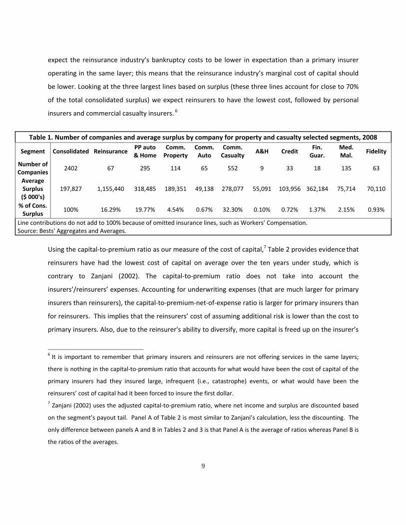
Reinsurers often have better diversification opportunities than primary insurers if only because they do

not face the same regulatory oversight as primary insurers. Furthermore, they are generally larger global

entities (see Table 1) than primary insurers, thus allowing them to gain access to a much wider set of

potential sources of risk whose losses are presumably less correlated, thus increasing their potential for

diversifying their losses. We show in Table 1 that U.S. reinsurers have substantially more surplus per

company (more than 300% larger than the next largest segment) than any other segment U.S. insurers.

Reinsurers domiciled in the United States hold more than 16% of the total industry’s surplus, which

makes the U.S. reinsurance industry as a whole the third largest holder of surplus in the U.S. insurance

industry behind commercial casualty insurers (32% of total surplus) and personal automobile and

homeowner insurers (20% of total surplus).5 Because of the sheer size of each reinsurer, we should

5 The importance of reinsurers’ surplus would have been much larger had we taken an earlier year since 2008 was

a bad year for reinsurers.

9

expect the reinsurance industry’s bankruptcy costs to be lower in expectation than a primary insurer

operating in the same layer; this means that the reinsurance industry’s marginal cost of capital should

be lower. Looking at the three largest lines based on surplus (these three lines account for close to 70%

of the total consolidated surplus) we expect reinsurers to have the lowest cost, followed by personal

insurers and commercial casualty insurers. 6

Table 1. Number of companies and average surplus by company for property and casualty selected segments, 2008

Segment Consolidated Reinsurance PP auto & Home

Comm. Property

Comm. Auto

Comm. Casualty

A&H Credit Fin. Guar.

Med. Mal.

Fidelity

Number of Companies

2402 67 295 114 65 552 9 33 18 135 63

Average Surplus ($ 000's)

197,827 1,155,440 318,485 189,351 49,138 278,077 55,091 103,956 362,184 75,714 70,110

% of Cons. Surplus

100% 16.29% 19.77% 4.54% 0.67% 32.30% 0.10% 0.72% 1.37% 2.15% 0.93%

Line contributions do not add to 100% because of omitted insurance lines, such as Workers’ Compensation. Source: Bests' Aggregates and Averages.

Using the capital‐to‐premium ratio as our measure of the cost of capital,7 Table 2 provides evidence that

reinsurers have had the lowest cost of capital on average over the ten years under study, which is

contrary to Zanjani (2002). The capital‐to‐premium ratio does not take into account the

insurers’/reinsurers’ expenses. Accounting for underwriting expenses (that are much larger for primary

insurers than reinsurers), the capital‐to‐premium‐net‐of‐expense ratio is larger for primary insurers than

for reinsurers. This implies that the reinsurers’ cost of assuming additional risk is lower than the cost to

primary insurers. Also, due to the reinsurer's ability to diversify, more capital is freed up on the insurer’s

6 It is important to remember that primary insurers and reinsurers are not offering services in the same layers;

there is nothing in the capital‐to‐premium ratio that accounts for what would have been the cost of capital of the

primary insurers had they insured large, infrequent (i.e., catastrophe) events, or what would have been the

reinsurers’ cost of capital had it been forced to insure the first dollar.

7 Zanjani (2002) uses the adjusted capital‐to‐premium ratio, where net income and surplus are discounted based

on the segment’s payout tail. Panel A of Table 2 is most similar to Zanjani’s calculation, less the discounting. The

only difference between panels A and B in Tables 2 and 3 is that Panel A is the average of ratios whereas Panel B is

the ratios of the averages.

10

side than is bound on the reinsurer's side. Therefore, the cost of assuming the risk is lower for the

reinsurer than for the insurer.

Table 2. Capital‐to‐premium (or capital cost) ratios of selected property and casualty insurance segments

Panel A. Capital cost ratios by year (1999‐2008) and average of capital cost ratios

Fiscal year end

Consolidated Reinsurance PP auto & Home

Comm. Property

Comm. Auto

Comm. Casualty

A&H Credit Fin. Guar.Med. Mal.

Fidelity

2008 ‐7.0% ‐13.7% ‐3.9% ‐1.0% ‐1.0% 1.3% 26.1% ‐4.9% ‐373.1% 14.4% 26.3%

2007 12.2% 21.1% 8.6% 17.5% 7.0% 14.1% 14.6% 16.1% ‐40.0% 23.9% 22.8%

2006 17.2% 35.7% 13.1% 17.9% 7.6% 24.3% 5.8% 14.9% 106.8% 20.0% 18.3%

2005 10.6% 4.0% 9.0% 18.5% 5.3% 7.6% 37.9% 14.0% 89.8% 9.6% 17.9%

2004 9.8% 11.0% 10.0% 12.5% 5.0% 6.9% 12.5% 10.6% 78.2% ‐1.3% 15.4%

2003 9.6% 20.3% 7.6% 15.4% 8.4% 4.7% 9.4% 16.1% 72.0% ‐4.3% 10.6%

2002 ‐5.0% ‐12.1% ‐6.5% 4.6% 7.9% ‐4.9% 6.3% 10.7% 66.9% ‐25.5% 1.9%

2001 ‐10.1% ‐30.1% ‐11.1% ‐9.7% 9.4% ‐9.1% 4.2% 4.0% 77.5% ‐17.9% 3.0%

2000 ‐2.6% ‐5.4% ‐6.3% ‐0.5% 11.0% 0.3% 1.1% 5.5% 92.6% ‐7.4% 4.0%

1999 2.5% ‐9.8% 2.8% ‐9.7% 3.1% 2.7% ‐7.3% 6.3% 103.4% 1.0% 9.6%

10‐year average

3.7% 2.1% 2.3% 6.6% 6.4% 4.8% 11.1% 9.3% 27.4% 1.3% 13.0%

The Capital Cost Ratio is calculated as (Net Income + Unrealized Capital Gains + Income Taxes – Investment Income) / (Direct Premium Written + Policyholder Dividends – Investment Income); Investment Income is calculated as Return on Investment * Surplus. Source: Bests' Aggregates and Averages.

Panel B. Capital cost ratio averages (1999‐2008)

Year Consolidated Reinsurance PP auto & Home

Comm. Property

Comm. Auto

Comm. Casualty

A&H Credit Fin. Guar. (ex 2008)

Med. Mal.

Fidelity

10‐year average

4.0% 1.0% 2.6% 9.3% 5.4% 5.6% 5.4% 8.3% 64.3% 3.1% 16.1%

The Average Capital Cost Ratio is calculated as (10 year Total Net Income + 10 year Total Unrealized Capital Gains + 10 year Total Income Taxes – 10 year Total Investment Income) / (10 year Total Direct Premium Written + 10 year Total Policyholder Dividends – 10 year Total Investment Income); Investment Income is calculated as Return on Investment * Surplus. Source: Bests' Aggregates and Averages.

When expenses are taken into account in Table 3, reinsurers still have on average a lower capital cost.

Clearly, including expenses in the capital‐to‐premium ratio calculations increases the capital costs for all

segments, but less so for reinsurance than for other segments, as we anticipated. The reason is that

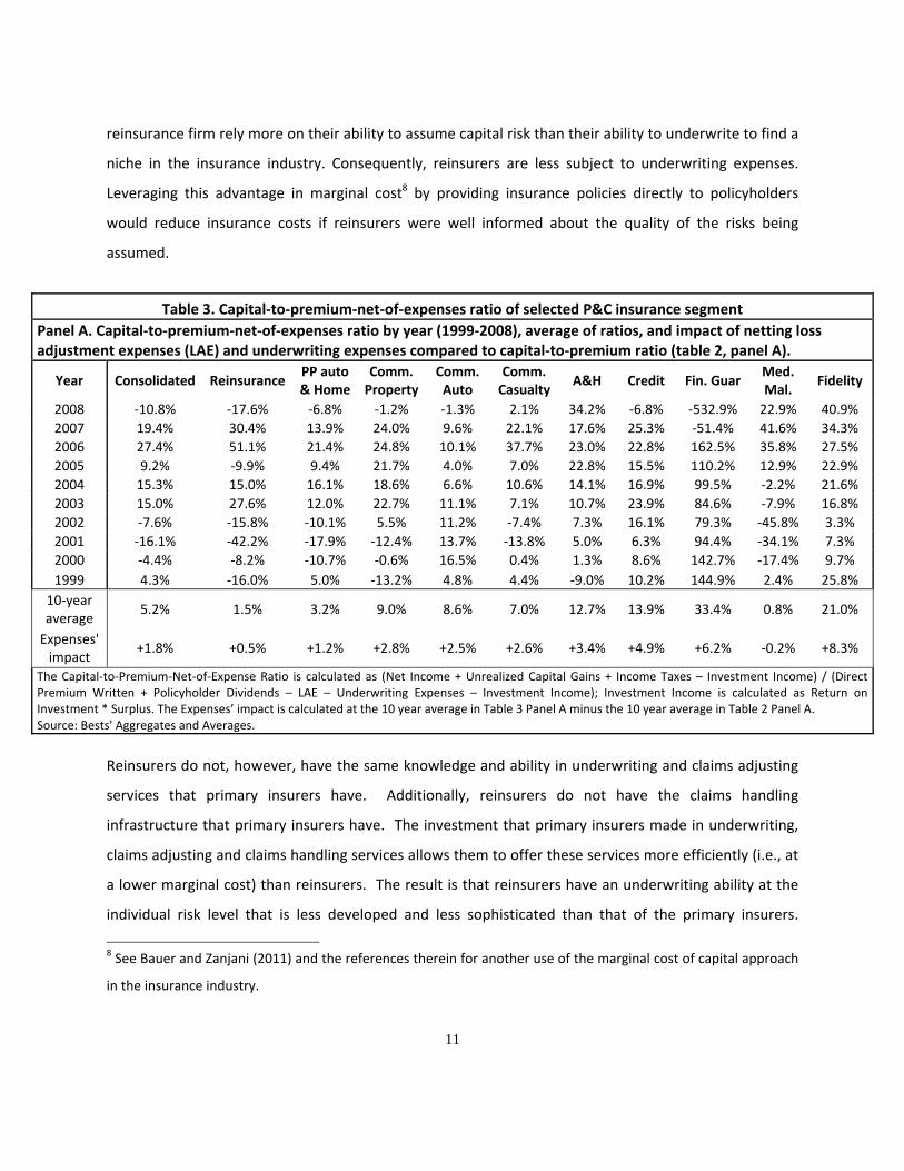
11

reinsurance firm rely more on their ability to assume capital risk than their ability to underwrite to find a

niche in the insurance industry. Consequently, reinsurers are less subject to underwriting expenses.

Leveraging this advantage in marginal cost8 by providing insurance policies directly to policyholders

would reduce insurance costs if reinsurers were well informed about the quality of the risks being

assumed.

Table 3. Capital‐to‐premium‐net‐of‐expenses ratio of selected P&C insurance segment

Panel A. Capital‐to‐premium‐net‐of‐expenses ratio by year (1999‐2008), average of ratios, and impact of netting loss adjustment expenses (LAE) and underwriting expenses compared to capital‐to‐premium ratio (table 2, panel A).


Comm. Property

Comm. Auto

Comm. Casualty

A&H Credit Fin. Guar Med. Mal.

Fidelity

2008 ‐10.8% ‐17.6% ‐6.8% ‐1.2% ‐1.3% 2.1% 34.2% ‐6.8% ‐532.9% 22.9% 40.9%

2007 19.4% 30.4% 13.9% 24.0% 9.6% 22.1% 17.6% 25.3% ‐51.4% 41.6% 34.3%

2006 27.4% 51.1% 21.4% 24.8% 10.1% 37.7% 23.0% 22.8% 162.5% 35.8% 27.5%

2005 9.2% ‐9.9% 9.4% 21.7% 4.0% 7.0% 22.8% 15.5% 110.2% 12.9% 22.9%

2004 15.3% 15.0% 16.1% 18.6% 6.6% 10.6% 14.1% 16.9% 99.5% ‐2.2% 21.6%

2003 15.0% 27.6% 12.0% 22.7% 11.1% 7.1% 10.7% 23.9% 84.6% ‐7.9% 16.8%

2002 ‐7.6% ‐15.8% ‐10.1% 5.5% 11.2% ‐7.4% 7.3% 16.1% 79.3% ‐45.8% 3.3%

2001 ‐16.1% ‐42.2% ‐17.9% ‐12.4% 13.7% ‐13.8% 5.0% 6.3% 94.4% ‐34.1% 7.3%

2000 ‐4.4% ‐8.2% ‐10.7% ‐0.6% 16.5% 0.4% 1.3% 8.6% 142.7% ‐17.4% 9.7%

1999 4.3% ‐16.0% 5.0% ‐13.2% 4.8% 4.4% ‐9.0% 10.2% 144.9% 2.4% 25.8%

10‐year average

5.2% 1.5% 3.2% 9.0% 8.6% 7.0% 12.7% 13.9% 33.4% 0.8% 21.0%

Expenses' impact

+1.8% +0.5% +1.2% +2.8% +2.5% +2.6% +3.4% +4.9% +6.2% ‐0.2% +8.3%

The Capital‐to‐Premium‐Net‐of‐Expense Ratio is calculated as (Net Income + Unrealized Capital Gains + Income Taxes – Investment Income) / (Direct Premium Written + Policyholder Dividends – LAE – Underwriting Expenses – Investment Income); Investment Income is calculated as Return on Investment * Surplus. The Expenses’ impact is calculated at the 10 year average in Table 3 Panel A minus the 10 year average in Table 2 Panel A. Source: Bests' Aggregates and Averages.

Reinsurers do not, however, have the same knowledge and ability in underwriting and claims adjusting

services that primary insurers have. Additionally, reinsurers do not have the claims handling

infrastructure that primary insurers have. The investment that primary insurers made in underwriting,

claims adjusting and claims handling services allows them to offer these services more efficiently (i.e., at

a lower marginal cost) than reinsurers. The result is that reinsurers have an underwriting ability at the

individual risk level that is less developed and less sophisticated than that of the primary insurers.

8 See Bauer and Zanjani (2011) and the references therein for another use of the marginal cost of capital approach

in the insurance industry.

12

Assuming transaction costs are low, the use of a reinsurance contract with a proper attachment point

should combine the primary insurers’ efficiency in underwriting and claims adjusting services with the

reinsurers’ comparative advantage at obtaining capital at low cost for very large exposures.

Panel B. Capital‐to‐premium‐net‐of‐expenses ratio averages (1999‐2008) and impact of netting loss adjustment expenses (LAE) and underwriting expenses compared to capital‐to‐premium ratio (table 2, panel B).


Comm. Property

Comm. Auto

Comm. Casualty

A&H Credit Fin. Guar. (ex 2008)

Med. Mal.

Fidelity

10‐year average

6.2% 1.4% 4.3% 12.5% 7.5% 8.7% 6.5% 12.6% 82.8% 5.6% 25.4%

Expenses' impact

+2.2% +0.4% +1.7% +3.2% +2.1% +3.1% +1.0% +4.3% +18.5% +2.5% +9.3%

The Capital‐to‐Premium‐Net of Expenses Ratio is calculated as (10 year Total Net Income + 10 year Total Unrealized Capital Gains + 10 year Total Income Taxes – 10 year Total Investment Income) / (10 year Total Direct Premium Written + 10 year Total Policyholder Dividends – 10 year LAE Expenses – 10 year Underwriting Expenses – 10 year Total Investment Income); Investment Income is calculated as Return on Investment * Surplus. The Expenses’ impact is calculated at the 10 year average in Table 3 Panel B minus the 10 year average in Table 2 Panel B. Source: Bests' Aggregates and Averages.

3.2. Modeling Strategy

Let us first posit that the total premium of the insurance contract includes the expected loss and any

other expenses related to marketing, underwriting, claims handling, and whatever risk premium is

needed to reward the providers of capital in this market. Let us also posit that the cost of the insurance

contract is made up of all costs in excess of the expected loss. Put differently, the premium is given by

YCYE ][ where E[Y] is the expected loss and C(Y) is the total cost of the insurance services. It

will become obvious later why we separate this cost of insurance services (that will include underwriting

and claims services as well as the implicit and explicit cost of capital requirements) from the pure

premium (or the expected economic loss), which we will assume is exogenously determined and must

be borne by someone in the economy. The loss Y is distributed according to some density function g(Y)

over the range ]ˆ,0[ YY , where Y is the maximum possible loss. We can therefore write the expected

loss as Y

dYYYgYEˆ

0

][ .

13

We will assume in our model that all policyholders (consumers with property exposed to catastrophic

risk) are trying to minimize the total cost of their insurance contract. We will assume that the total cost

of insurance services, C(Y), has two components: insurer expenses (the underwriting and claims

administrative costs, including loss adjustment expenses) and the cost of bearing the risk. It is the

relationship between these two cost components (the underwriting cost and the cost of bearing the

risk) that determines the insurance/reinsurance contract structure.

The model assumes there are N potential entities that could sell insurance protection in a competitive

market, where the price of insurance is equal to its marginal cost (see Zanjani, 2002, and Froot and

O’Connell, 2008). For simplicity, assume that each of these entities is characterized by a linear marginal

cost9 of providing coverage in the event of a catastrophic loss. The marginal cost function we use

depends on the insurer’s cost of capital (which we shall denote k) and its underwriting and claims‐

handling ability (which we shall denote b). For any of these entities, n, the marginal cost associated with

a possible loss of magnitude Y is a linear function with two parameters, given by Equation 1 and

illustrated in Figure 3.1.

YkbYC nnn | (1)

with ]ˆ,0[ YY where Y is the maximum possible loss. Entities in the economy differ with respect to

their nb ’s and nk ’s as determined by the entity’s production function (discussed later).

The intercept of the marginal cost function is equal to the cost of underwriting since the price of labor

should not vary with the size of the risk, in contrast to the cost of capital that increases with the size of

the risk. The policyholder’s goal is to find the policy that minimizes the total cost of insuring against a

possible loss Y . In other words, the policyholder chooses an insurance contract, or a set of insurance

9 Froot and O’Connell (2008) also use a linear marginal cost of providing hedging (i.e., reinsurance) services as an

intermediary good (see Dionne et al. 2010 for an alternative model of hedging as an intermediary good). The

marginal cost does not need to be a linear function of the maximum possible loss; the results will hold as long as

the marginal cost remains an increasing function of the maximum possible loss.

14

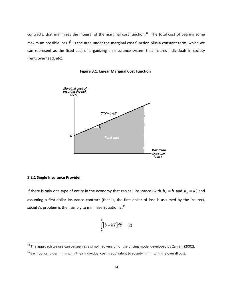
contracts, that minimizes the integral of the marginal cost function.10 The total cost of bearing some

maximum possible loss Y is the area under the marginal cost function plus a constant term, which we

can represent as the fixed cost of organizing an insurance system that insures individuals in society

(rent, overhead, etc).

Figure 3.1: Linear Marginal Cost Function

3.2.1 Single Insurance Provider

If there is only one type of entity in the economy that can sell insurance (with bbn and kkn ) and

assuming a first‐dollar insurance contract (that is, the first dollar of loss is assumed by the insurer),

society’s problem is then simply to minimize Equation 2.11

YdkYbY

ˆ

0

(2)

10 The approach we use can be seen as a simplified version of the pricing model developed by Zanjani (2002).

11 Each policyholder minimizing their individual cost is equivalent to society minimizing the overall cost.

15

The premium charged by the single provider would then be

YdkYbYYgYdkYbdYYYgYCYEYYY

ˆ

0

ˆ

0

ˆ

0

][ (3)

In the case of a more general marginal cost function, say a convex function given by YfbYC | ,

with 0| Yf and 0|| Yf , the total premium would be equal to YdYfbYYgY

ˆ

0

.

3.2.2 Two Insurance Providers

Now suppose there are two entities n1 and n2 such that 21 bb and 21 kk . This means that entity n1’s

marginal cost intercept is lower than entity n2’s. Put differently, entity n1 is able to provide underwriting

and claims service marginally cheaper than entity n2. However, each dollar of coverage (marginal cost of

capital) is more expensive for entity n1. The question becomes how to combine the two entities’

technology to minimize the total cost of the risk. Because one entity has a lower intercept but a higher

slope, a policyholder will minimize the total cost by dealing with the low‐intercept entity (better

underwriting and claims service) for lower losses and the low‐slope entity (lower marginal cost of

capital) for higher losses.

Graphically, we find that the total cost of bearing risk of potential loss Y is a combination of the two

entities: The low‐intercept entity is responsible for losses up until point y1 and the low‐slope entity is

responsible after point y1. Changing vocabulary12 to fit with the insurance industry’s we can say that

entity n1 is the primary insurer whereas entity n2 is the reinsurer that assumes losses greater than y1.

The question becomes: At what attachment point should the reinsurer become liable (i.e, what y1

minimizes the total cost of bearing this risk)? Abstracting from the expected loss component of the total

12 We change the vocabulary only to lighten the reading of the paper. We acknowledge that there are many types

of financial products that can replicate reinsurance. Albertini and Barrieu (2009) and Cummins and Weiss (2009)

provide examples of insurance‐linked securities and financial instruments that can adequately replace, in some

instances, an excess‐of‐loss or a proportional reinsurance contract.

16

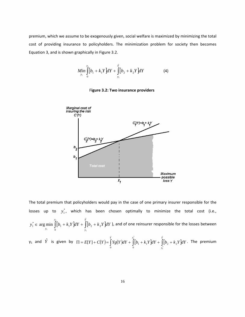
premium, which we assume to be exogenously given, social welfare is maximized by minimizing the total

cost of providing insurance to policyholders. The minimization problem for society then becomes

Equation 3, and is shown graphically in Figure 3.2.

Y

y

y

ydYYkbdYYkbMin

ˆ

22

0

11

1

1

1

(4)

Figure 3.2: Two insurance providers

The total premium that policyholders would pay in the case of one primary insurer responsible for the

losses up to *1y , which has been chosen optimally to minimize the total cost (i.e.,

Y

y

y

ydYYkbdYYkby

ˆ

22

0

11*1

1

1

1

minarg ), and of one reinsurer responsible for the losses between

y1 and Y is given by Y

y

yY

dYYkbdYYkbdYYYgYCYEˆ

22

0

11

ˆ

0 *1

*1

][ . The premium

17

collected by the reinsurer is Y

y

Y

y

R dYYkbdYYYgˆ

22

ˆ

*1

*1

. The amount saved ( R ) by having losses

greater than *1y reinsured instead of having all the risk being borne by the primary insurer is given by

Y

y

yYYY

R dYYkbdYYkbdYYYgdYYkbdYYYgˆ

22

0

11

ˆ

0

ˆ

0

11

ˆ

0 *1

*1

(5)

More concisely savings are equal to Y

y

Y

y

Y

y

R dYYkkbbdYYkbdYYkbˆ

2121

ˆ

22

ˆ

11*1

*1

*1

. If

the property owner chooses to retain the first portion of the risk (a deductible) and then insure above

that point, the function to minimize would then simply be equation 6,

ydykbydykbMinY

d

d

d ˆ

11

0

00 (6)

In Equation 6, we let d represent the deductible and replaces y1 when comparing to equation 4. We can

therefore see this case as that of a policyholder who becomes the first‐dollar insurer who then reinsures

the risk with what we have called the primary insurer. The total premium paid by the policyholder would

then be given by what we previously called the reinsurer’s premium, Y

d

Y

d

R dYYkbdYYYgˆ

22

ˆ

,

where the attachment point 1y is replaced by the deductible d. The implicit total premium paid by the

policyholder is not only that paid to the insurer, but also includes the portion that the policyholder

retains. Consequently, the total premium‐cum‐cost for society does not change and remains

Y

d

dY

dYYkbdYYkbdYYYgˆ

11

0

00

ˆ

0

, where the index 0 represents the policyholder’s

marginal cost function of bearing risk.

It is interesting to note that we have a new reason why deductible exists in a competitive environment.

Even with no adverse selection or moral hazard problems, because insurers have lower capital cost of

18

bearing risk than individuals (who are better equipped to assess their own risk), individuals will assume

the first few dollars of loss whereas insurers will step in as the providers of resources when losses are

greater than the threshold d found in equation 6.13

3.2.3 N Insurance Providers

Now suppose there are N entities such that Nbbb ...21 and Nkkk ...21 . This means that

entity n1’s marginal cost intercept is lower than entity n2’s, which is lower than n3’s, etc. Similarly, each

dollar of coverage (marginal cost of capital) is more expensive for entity n1 than for n2 than for n3 etc. As

before, the optimal combination of the N entities’ technology will be for the policyholder to deal with

the entity that has the lowest intercept first (it has the best underwriting and claims service technology),

and then reinsure at different layers when having a low marginal cost of capital becomes important.

Layers are determined by the comparative advantage of each reinsurer at assuming catastrophic losses

as shown in Figure 3.3.

Reinsurance in this economy “concavifies” the overall marginal cost function. By increasing the number

of entities (i.e. reinsurers) one increases the concavity of the marginal cost function and therefore

reduces total cost. The resulting curve in figure 3.3 could be thought of as a contract efficiency

(efficient‐C curve) curve. This curve could be used to compare actual insurance programs to this

minimum cost curve. The insurance contracts would lie up and to the left of this curve and a measure of

the efficiency loss would be the difference in the areas under the two curves. It would be possible to

determine at which points in the loss distribution inefficiencies are created and whether those

inefficiencies are due to capital (k) or labor (b) issues, or inefficient attachment points.

13 This still assumes some information asymmetry, but no residual asymmetry after underwriting expertise. If

there was no costly information, underwriting would not be costly, but claims handling would still be costly,

including some level of inefficiency. For very small losses, individuals can use their own capital (checking account,

line of credit or credit card) to handle small claims better than insurers.

19

Figure 3.3: N insurance entities

As the market allows more and more insurers that have different underwriting expertise (b) and risk‐

bearing capacities (k) the total cost to policyholders, still excluding the pure premium, is decreased. This

necessarily improves everyone’s welfare. If there are N private insurers and reinsurers such that

Nbbb ...21 and Nkkk ...21 , society’s cost minimization problem is equation 7.

N

i

y

y

ii

y

yy

i

iN

dYYkbdYYkbMin20

11,...

1

1

1

(7)

There are two types of equilibriums that can be evaluated from this model. The first is an exogenous

equilibrium where the b’s and k’s for insurers are determined exogenously. The second is an

endogenous equilibrium where the b’s and k’s are determined through a production function.

3.3 An Exogenous Equilibrium

Clearly the equilibrium on this market will depend on how the parameter values ib and ik of all private

insurers and reinsurers are distributed in the economy. Suppose there are two insurers, insurer h with

20

hb and hk , and insurer j with jb and jk . If jh bb and jh kk , then cost minimization will be

obtained by having only one insurer. In other words, insurer h here dominates insurer j for every type of

loss: It has better underwriting expertise and a lower cost of bearing risk. In an efficient market, insurer j

would find itself filing for bankruptcy.

Suppose now that jh bb and jh kk so that both insurers have the same risk bearing technology, but

one insurer (insurer h) has a better underwriting expertise than the other. In other words, one insurer

can do the same underwriting job, but at a lower cost. Again, insurer j would find itself filing for

bankruptcy since it has a more costly production function that insurer h. A similar story can be told if

jh bb and jh kk , so that both insurers have the same underwriting ability, but one insurer (insurer

h) has a better ability to assume large losses that the other insurer in the sense that insurer h’s cost of

assuming the risk is lower. Clearly insurer j would find itself filing for bankruptcy, again, since it has a

more costly production function that insurer h.

For an excess‐of‐loss reinsurance market to exist in equilibrium, it therefore has to be that the

reinsurers’ marginal cost functions have a higher intercept and a lower slope. If this is not the case, then

the entire potential loss of a policyholder will be assumed by a single unique insurer. In reality, we know

that primary insurers rely on reinsurers to guarantee eventual indemnity payments for the highest levels

of potential losses. Consequently, in the absence of market imperfections a policyholder’s loss will be

handled by more than one entity only if reinsurers have a lower cost of bearing large risks than primary

insurers.

Assume now that the two insurers have the same b and the same k. If two insurers have the same

marginal cost function, this means that there is no value in excess of loss reinsurance since there is no

efficiency gain. The primary insurance market would then, on average, be split between the two insurers

who are both offering the insurance service at the lowest possible marginal cost to the policyholders.

Imagine that there is a third entity in this market that has a lower b and a higher k than these two. If that

is the case, then the new entity would become the primary insurer (having the lowest intercept) and the

two others would become reinsurers that each receives half of the primary insurer’s business. One can

21

imagine that this fits the description, from the point of view or the reinsurer, of a proportional

reinsurance contract with each reinsurer assuming 50% of the lost above the attachment point (which is

sometimes referred to as corridor contracts). If instead of having a lower intercept the third entity has a

lower marginal cost slope (and a higher intercept) than the first two insurers, then the primary market

would be split equally between the two initial insurers and both would reinsure their higher losses with

the new entity using an excess of loss contract.

By adding more insurance entities that have different b’s and k’s generates a market equilibrium where

primary insurers are those that have the lowest b’s and reinsurer involvement through excess‐of‐loss

contracts depends on the right combination of b’s and k’s, with the reinsurer with the lowest k and the

highest b assuming the highest tranche. If two or more entities have the same b and the same k, then

they split equally the tranche in which they belong in the marginal cost hierarchy (see the appendix for

the illustration using an insurance program chart).

If there are market imperfections, such as search, transactions and intermediary costs,14 then it is quite

possible that the optimal structure that minimizes total cost is not obtained. It nonetheless remains

theoretically feasible to find the combination of insurers and reinsurers that minimizes the total cost of

supporting catastrophic risk. Whether this optimal combination is observed in reality or not becomes an

empirical question that can be answered in a companion paper. Consequently, insurers that want to

insure a given tranche must balance the higher cost of capital of assuming a large tranche with the

benefit of having lower volatility (see Tasche, 2004, Zanjani, 2010, and Bauer and Zanjani, 2011, for a

similar idea in the case of risk capital).

14 To be fair, there have been numerous explanations for the limited sharing of catastrophe risk that involve some

type of market imperfection such as: 1‐adverse selection and moral hazard problems in the reinsurance market as

in Niehaus and Mann (1992); 2‐ corporate taxes as in Jaffe and Russell (1997), Harrington and Niehaus (2003) and

Zanjani (2002); 3‐ tail risk and in Bernard and Tian (2009); and 4‐ barriers to capital Froot and O'Connell (1999) and

Froot (2001).

22

3.4 An Endogenous Equilibrium

3.4.1 An Insurance/Reinsurance Production Function

How firms decide to offer insurance service as a primary insurer or as a reinsurer, and as what type of

reinsurer (high attachment point or low attachment point insurer) remains an open question. In the

previous section we just assumed that some entities had high b’s and low k’s (the reinsurers typically)

whereas others had low b’s and high k’s (the primary insurers typically) determined exogenously.

Suppose that the genesis of the insurance market is populated by a set of entities that all have access to

the same technology that is given by some function nn LKLKTn 1, for Nn ,...,1 . For

simplicity let us assume a constant elasticity of substitution production function. All entities want to

maximize their value by choosing the right amount of capital Kn and labor Ln,.15 Entities differ only with

respect to the parameter 1,0n . Assume that all entities start with the same level of surplus, S

(which we could also see as their available capacity – see Zanjani, 2010, for more in the marginal use

and cost of capital in an insurance company). The price of capital is given by pK, which we will assume

constant for a given level of capital, and the price of labor is given by pL, which will always be constant

per unit of labor. Consequently, an entity n will choose a level of labor and capital that at most uses the

entire insurer’s available surplus so that SLpKp nLnk ** . As entities are endowed with technology

that allows them to be more or less efficient in the use of labor or capital (the parameter varies from

one entity to the next), they will opt to invest more in one and less in the other. A firm’s problem can

then be written as a choice between investment in capital and investment in labor that maximizes firm

value:

SLpKptsLKLKT nLnknnnLK

nn

nn

..,max 1

,

. (8)

15 As it will become apparent later, we should view labor as the investment an insurer makes in the underwriting

and the claims handling abilities of its employees whereas capital should be viewed as its investment in optimizing

its capital structure, ability to pool individual risks, diversify risk by line of business and geographically, and attract

capital to meet the current level of risk it seeks to assume.

23

The solution to this problem is straightforward. 16 Firm value is maximized when the amount invested in

labor and in capital is such that

SP

LL

nn

1* and SP

KK

nn

* .

We see that as the parameter n becomes larger, an entity will invest more in capital. At the other end

of the spectrum, a low parameter n means that the entity has a better underwriting technology and

therefore will invest more in the labor component.

An alternative modeling approach would be to see S as the amount of economic capital needed to

support a given risk. In a CAPM world, we know that for a given risk, the amount of economic capital

needed is independent of the insurer since it depends only on the covariance of the risk with the market

portfolio. The same is true in a reinsurance context as shown in Borch (1962). This alternative approach

allows for the modeling of each risk individually so that (re)insurance entities are allowed to assume

different layers for different risks. To see why, we could let the parameter 1,0, mn be different for

each risk m that requires surplus mS to underwrite. Since the choice of capital and labor is made for

each risk individually as a function of the surplus that is required and the (re)insurer’s production

function, (re)insurers could make different capital and labor choices as a function of the type of risk.

3.4.2 Returning to the Marginal Cost Function

Letting *

1

nn

Lb and

*

1

nn

Kk 17 in the marginal cost equation we had before, we see that an entity

that is endowed with a higher n parameter will have a marginal cost function that has higher intercept

16 The first order conditions write 011

knnn pLK nn and 01 Lnnn pLK nn . Solving we find a

Lagrange multiplier equal to Kn

nn

Ln

nn pL

K

pL

Ka

nn

111

1

. This yields an optimal choice of capital

and labor such that

K

Ln

n

nn p

PLK

1

and n

L

k

Ln K

P

pS

PL

1 . Solving for Kn and Ln completes the exercise.

24

and a lower slope, the type of cost function that one should observe in a reinsurer. The opposite also fits

our model as firms whose parameter n is small will be more likely to become primary insurers since

their marginal cost function will have a lower intercept and a higher slope.

An interesting aspect of this insurance production function is that we can see that a sudden increase in

the unit price of capital (pk) will reduce the amount of capital that every entity uses, but it will not affect

the amount of labor used. This means that as we transpose the production function into the cost

function that society wants to minimize, a capital shock does not alter the intercept of the marginal cost

function, but it does increase its slope, consistent with an increase in the capital cost of bearing large

risks. This impact will be larger for companies that already invest a lot in the capital component of the

production function (that is, the reinsurers). To see why, note that

02

*

Spp

K

K

n

K

n . As we know

from an earlier discussion, entities that have a large n parameter are those that invest more in capital,

and that are more likely to be reinsurers. It then follows that large n entities (i.e., the reinsurers) will

be more affected by capital price shocks than primary insurers, which is consistent with industry stylized

facts as well as the literature on reinsurance capital (see Berger et al., 1992).

Following our particular setup, we can write that YCn| is a function of labor and capital so that

YS

P

S

PYkbYC

n

K

n

Lnnn

1

|. The comparative static shows that an increase in the price of

labor increases the intercept whereas an increase in the price of capital increases the slope. Interestingly

as well, an increase in the “capital intensity” parameter (αn) gives us a higher intercept and a lower

slope. Finally, larger firms, as measured by their surplus, should have a lower intercept and a lower

slope, suggesting that larger firms are better both at the underwriting end of the business and at the risk

bearing end if they were to allocate their entire capital surplus to a single risk or line. In other words,

there is an economy of scale. But as large insurers operate in more than one line of business (however

17 This assumes that investing more in labor (capital) lowers the marginal cost of providing labor (capital) to the

policyholders.

25

we define a line of business, by type of risk or even geographically) what is allocated to a given line will

not represent 100% of the larger insurer’s surplus capital. Smaller insurers could probably allocate close

100% of their surplus capital to a single line or even risk. Consequently, even though larger insurers

could be more efficient in each line of business, one must wonder in what line – following David

Ricardo’s terminology – larger insurers have a comparative advantage over other insurers.

The advantage of the production function we have used is that it turns a two‐parameter (bn and kn) firm‐

specific marginal cost problem into a one‐parameter firm‐specific problem (αn) without altering the

desired properties of the distribution of the marginal cost functions. In other words, if we were to rank

the firms according to the parameter αn so that N ...21 , we would have that Nbbb ...21

and Nkkk ...21 . This means that the greater the “capital intensity” parameter (αn), the higher is

the intercept and the lower the slope. Consequently, firms that have a higher ability to use capital (i.e.,

firms that have a higher αn), should become reinsurers.

A second important advantage of the production function we have chosen is that surplus is additive over

the different lines of business. In other words, assuming there are M lines, firm n’s total surplus is given

by m

mnn SS , . Allowing firms to have parameters αn,m that differs across lines, the total amount spent

in labor (resp. capital) by the firm would then be

m

mnmL

mn

mmnn S

PLL ,

,

,,

1 (resp.

m

mnmK

mn

mmnn S

PKK ,

,

,,

) where we assumed that labor costs (resp. capital costs) are line specific.

Size would then matter somewhat less. 18

18 This is in the spirit of economic capital allocation whereby one would like to allocate capital to lines of business

according to their marginal impact.

26

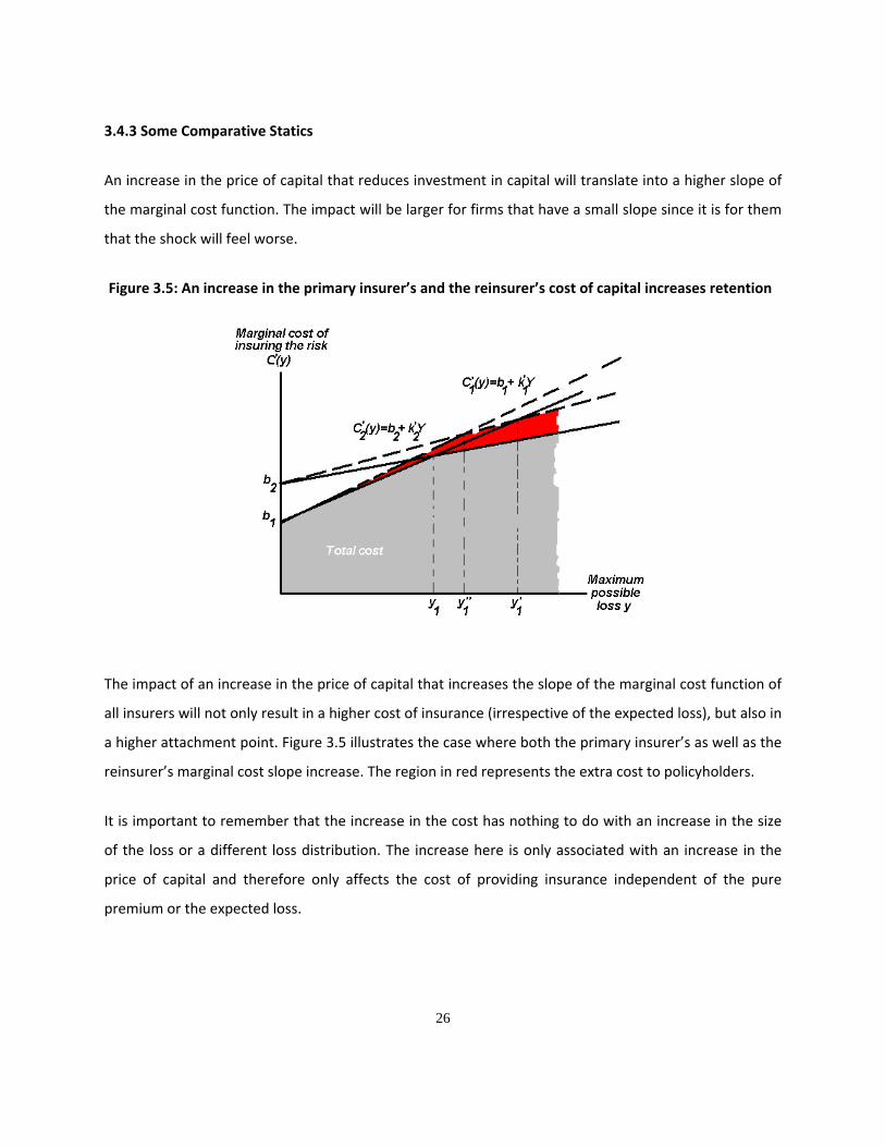
3.4.3 Some Comparative Statics

An increase in the price of capital that reduces investment in capital will translate into a higher slope of

the marginal cost function. The impact will be larger for firms that have a small slope since it is for them

that the shock will feel worse.

Figure 3.5: An increase in the primary insurer’s and the reinsurer’s cost of capital increases retention

The impact of an increase in the price of capital that increases the slope of the marginal cost function of

all insurers will not only result in a higher cost of insurance (irrespective of the expected loss), but also in

a higher attachment point. Figure 3.5 illustrates the case where both the primary insurer’s as well as the

reinsurer’s marginal cost slope increase. The region in red represents the extra cost to policyholders.

It is important to remember that the increase in the cost has nothing to do with an increase in the size

of the loss or a different loss distribution. The increase here is only associated with an increase in the

price of capital and therefore only affects the cost of providing insurance independent of the pure

premium or the expected loss.

27

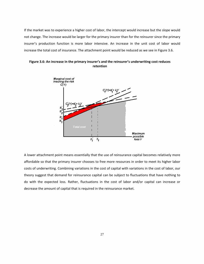
If the market was to experience a higher cost of labor, the intercept would increase but the slope would

not change. The increase would be larger for the primary insurer than for the reinsurer since the primary

insurer’s production function is more labor intensive. An increase in the unit cost of labor would

increase the total cost of insurance. The attachment point would be reduced as we see in Figure 3.6.

Figure 3.6: An increase in the primary insurer’s and the reinsurer’s underwriting cost reduces retention

A lower attachment point means essentially that the use of reinsurance capital becomes relatively more

affordable so that the primary insurer chooses to free more resources in order to meet its higher labor

costs of underwriting. Combining variations in the cost of capital with variations in the cost of labor, our

theory suggest that demand for reinsurance capital can be subject to fluctuations that have nothing to

do with the expected loss. Rather, fluctuations in the cost of labor and/or capital can increase or

decrease the amount of capital that is required in the reinsurance market.

28

4. AN APPLICATION TO PUBLIC INTERVENTION

4.1 The Role of Government as an Insurance Provider

In this model, government entities can enter as insurance entities. We are assuming that a government

entity has the lowest cost of raising capital through its ability to tax (so it has the lowest marginal cost of

bearing risk, kg) but it has the highest underwriting cost since it has no expertise in the matter (so it has

the highest intercept, bg). Because the state has the lowest marginal cost of bearing risk, it is natural

that it would enter the insurance market as the reinsurer of last resort (see Kessler, 2008, for other

reasons). Expanding the two‐provider model with the third entity being a government insurance

provider, we learn that the problem for society is to find the reinsurer’s appropriate attachment point y1

and detachment point y2 such that we still minimize the total cost as shown in equation 9 and

graphically in Figure 4.1.

ydykbydykbydykbMinY

y

gg

y

y

y

yy ˆ

22

0

11,

2

2

1

1

21

. (9)

If reinsurance is not allowed, but government is still there as a reinsurer of last resort, the total cost

would be higher by an amount that is represented in the graph by the yellow triangle. The government’s

marginal contribution to the reduction in total cost can also be measured as the lined area in red on the

graph. Without the government as a reinsurer of last resort, private reinsurers would have to assume

the risk from attachment point y1 until the maximum possible loss Y . Thus, the total cost to insuring the

loss would be greater by an amount that is represented by the lined red triangle.

29

Figure 4.1: Government Entity as Insurer

If there are N private insurers and reinsurers such that b1<b2<…<bN and k1>k2>…>kN, and a government,

whose parameters are bg and kg such that bN<bg and kN>kg, that acts as a reinsurer of last resort,

society’s cost minimization problem becomes equation 10.

ydykbydykbydykbMinY

y

gg

N

i

y

y

ii

y

yyN

i

iN

ˆ

20

11,...

1

1

1

(10)

Government intervention is not considered free in our model. The premium governments should charge

to the insurance market is given by ydykbdYYYgY

Y

gg

Y

Y

g

NN

ˆˆ

. The benefit to society is then

given by an equation similar to equation 5:

N

i

y

y

ii

yY

y

gg

N

i

y

y

ii

y

G ydykbydykbydykbydykbydykbi

iN

i

i20

11

ˆ

20

11

1

1

1

1

(11)

30

More concisely, the benefit to efficient government intervention is Y

Y

GNGNG

N

dYYkkbbˆ

.

4.2 Public Policy Implications when Agents Have Heterogenous Cost Functions

The question in terms of public policy will be to assess the parameter values bi and ki of all private

insurers and reinsurers, as well as the government’s, so that the government’s optimal attachment point

can be determined. With this type of model, where competition in the primary layer and working layers

of reinsurance are dominated by firms with better underwriting and claims adjusting capabilities, there

are no advantages to having a government entity provide insurance coverage. It is also possible that

there is no point for government to become involved in the insurance market as a reinsurance of last

resort if, for instance, we find that cost minimization is obtained in the private market because the

solution would demand that YyNˆ . However, as the maximum possible loss increases, it becomes

more likely that a government entity is needed in the market as its lower cost of capital begins to

outweigh its inability to underwrite and manage claims.

The question of government intervention cannot be studied independently of the distribution of risk in

the economy. In the model so far, all individuals face the same risk, which means that government

intervention has no ex‐ante redistribution impact. As a result, provided that at some level the

government’s cost of capital is lower than the reinsurers’ lowest, government intervention increases

welfare. Suppose now that agents in the economy are heterogeneous with respect to the cost of

providing them with insurance. Put differently, suppose that there is a proportion of agents (with

1

) whose total cost of insurance services is given by YC . All agents still face the same

expected loss, but some are more costly to insure.

Using the case of one primary insurer, one reinsurer and government (who cost of capital is

independent of the private market’s cost function), the problem to minimize becomes

31

ydykbydykbydykbMinY

y

gg

y

y

y

yyg

g

g ˆ

22

0

11,

1

1

1

,

where the superscript represent the agents’ “cost type”, and the subscript g refers to the situation

facing the government. The optimal contract that minimizes the total cost of insurance will differ from

one agent type to the next as the attachment and detachment points will not be the same for every

contract, which is represented in the minimization function by the superscript on the attachment and

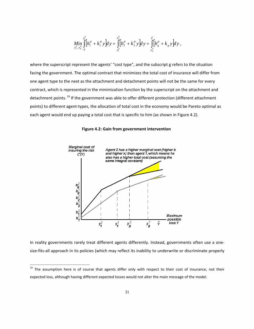
detachment points. 19 If the government was able to offer different protection (different attachment

points) to different agent‐types, the allocation of total cost in the economy would be Pareto optimal as

each agent would end up paying a total cost that is specific to him (as shown in Figure 4.2).

Figure 4.2: Gain from government intervention

In reality governments rarely treat different agents differently. Instead, governments often use a one‐

size‐fits‐all approach in its policies (which may reflect its inability to underwrite or discriminate properly

19 The assumption here is of course that agents differ only with respect to their cost of insurance, not their

expected loss, although having different expected losses would not alter the main message of the model.

32

across types). Since most government sponsored property casualty insurance programs involve some

subsidization of high risk exposures, there are also redistributive questions that need to be addressed.

In Florida (see Nyce and Maroney, 2011), inland homeowners subsidize homeowners who live on the

coast, and even properties slightly inland in the coastal area are subsidizing properties that are directly

on the ocean. Although we concentrate in this paper only on the total cost associated with insuring the

risks and not on the expected loss, we realize that premium subsidies include both the cost of insurance

(as we defined it in the current paper) as well as the expected loss. We will examine the case of agent

loss heterogeneity (with respect to the maximum possible loss, not their expected loss) in a later

section.

There are two types of government involvement that would induce redistribution problems. In the first

intervention, we will assume that government intervenes at the same level of loss for all agent types

(that is, the government’s attachment point is the same for all). In the second, we will assume that

government charges the same marginal cost to all the agents. In other words, the government sets

parameters bg and kg to be the same for all agents, and are therefore independent of . The

redistribution aspect of insurance contracts is highlighted in Kessler (2008) who writes that the “… very

rapid growth in the risk (government) covers … does not appear linked exclusively to the nature of the

risks … it results especially from the behavioral adaptation to what is considered … less and less as a risk

coverage and more and more as a right” (p. 6).

4.2.1 Same Government Protection (i.e., Same Attachment Point)

In the model, the government’s inability to discriminate results in every agent facing a government

attachment point of gy determined exogenously. Each agent‐type’s problem can then be written as

ydykbydykbydykbMinY

y

gg

y

y

y

yg

g

ˆ

ˆ

ˆ

22

0

11

1

1

1

(11)

33

As we see, government intervention fixes the upper attachment point gy so that it is no longer a choice

variable in the problem. If government fixes its attachment point gy between the optimal attachment

points of each type of agent, it is then easy to show that every agent ends up paying more for insurance

services. To see why, observe Figure 4.3 where we highlight the gains and losses (in terms of total costs)

to each type of agent arising from government intervention as a reinsurer of last resort.

Figure 4.3: Gain and loss from government intervention

The red wedges represent the extra cost imposed on each agent by having a fixed attachment point and

the yellow trapezes represent the gain to each agent for having government intervention. As we see, the

government’s attachment point gy lies between the two type specific (and optimal) attachment points

2gy and 1

gy . This means that, compared to the optimal type‐specific entry point, government intervenes

too early for the agents that have the lowest marginal cost (agent‐type 1 ) and too late for the agents

that have the higher marginal cost function (agent‐type 2 ). As a result, both types of agents end up

with a suboptimal situation. The loss of welfare for society is then given by the sum of the two areas

highlighted in red.

34

Interestingly, no government intervention that fixes its entry point (i.e., fix yg to be the same for all

agents) can be Pareto optimal. To see why, suppose that 2ˆ gg yy . The situation would then look like

that of Figure 4.4.

Figure 4.4: Government Intervention by fixing its attachment point below 2gy

As we can see, neither agent benefits from the government stepping in too early in the catastrophe risk

market. We therefore see that whatever attachment point the government fixes, heterogenous agents

can never be better off if the entry point is the same for all and if agents differ with respect to their

marginal cost function. The type of intervention we just examined presumes that the government

intervenes so that all agents receive the same “insurance” from the government entity after the loss has

occurred. Another possibility, and the one we examine next, is that government forces all agents to

share the cost of insurance equally so that the same underwriting cost is paid by all insured agents.

4.2.2 Same Marginal Cost of Government Insurance

The second type of redistribution the government can do is to forgo its ability to charge agents as a

function of their marginal cost type. Instead the government may use an “average” cost for all. Given

35

the way we have modeled the problem here, this means that the government inability to discriminate

results in every agent facing a government average “underwriting expertise cost” of

gg bb . The

problem for each agent‐type then becomes the following, and is illustrated in Figure 4.5

ydykbydykbydykbMinY

y

gg

y

y

y

yy ˆ

22

0

11,

2

2

1

1

21

ˆ

(12)

Figure 4.5: Government Intervention by assigning the same underwriting cost to all

By using the same intercept for all agents, the government’s attachment point for the high cost agents

(agent‐type 2) decreases, but is increases for the low cost agents (agent‐type 1). By doing so the high‐

cost agents are benefiting from the intervention, to the detriment of the low cost agent. Each high‐cost

agent’s decrease in total cost is given by the area in yellow. Each low‐cost agent’s increase in total cost is

given by the area in red. 20 The question, from society’s point of view, is whether the area in yellow (the

gain) is greater than the area in red (the loss), with each area weighted, of course, by the proportion of

20 Note that we do not let the government’s ability to raise money be a function of the agent‐type (we therefore

assume that the government’s financing, risk bearing and taxing abilities are independent of risk type).

36

each type of agents in society, . Surely, total welfare cannot increase given that the government

underwriting ability is a weighted function of its ability when faced with each agent separately.

We can combine the two types of intervention (same attachment point, same marginal cost function)

and examine how that affects the agents’ choice of insurance contracts. The problem then becomes

,ˆˆ

ˆ

ˆ

22

0

11

2

2

1

1

1

ydykbydykbydykbMinY

y

gg

y

y

y

y

where gb is defined as before as

gg bb .

Our presumption is that there will be a loss of welfare for society as a whole in the event that all risk

types share the same pooled fixed cost of underwriting because the state or the federal government

does not obey vertical equity precepts. In other words, not treating different risk types different leads to

a welfare loss. To see why, note that the gain for the high marginal cost agents (i.e., 2 ) is given by

the difference in the area under the curves from point '2gy until the maximum possible loss Y . In our

case, with one insurer, one reinsure and one government, the gain is given by

ydykbydykbydykbGainY

y

gg

Y

y

gg

y

y gg

g

g

ˆˆ

222

22

'22

2

'2

ˆ (13)

In the case of the low marginal cost agent (i.e., 1 ), his loss is given by the difference in the area

under the curves from point 1gy until the maximum possible loss Y . With one insurer, one reinsure and

one government, the loss is given by

ydykbydykbydykbLossY

y

gg

Y

y

gg

y

y gg

g

g

ˆ

1

ˆ

12

12

2'1

'1

1

ˆ (14)

Given the measure 1 of agents that lose and measure 12 1 of agents that gain, the question

then becomes whether Gain11 is greater or smaller than Loss1 . We can rewrite Gain and Loss as

yydkkyYbyYbyybGaing

g

y

y

ggggggg

2

'2

22

'222'2222

ˆˆˆ (13A)

37

yydkkyYbyYbyybLossg

g

y

y

ggggggg

'1

1

12

11'11'112

ˆˆˆ (14A)

We want to know the sign of LossGain 111 . Said differently, we want to know if the gain to the

ones outweighs the loss to the others. Note that for 1,01 , 01 11 LossGain , so that where

there is no one that gains (receives better treatment) or no one that loses, then the welfare gains and

losses are non existent. We want to know what happens for intermediate values of 1 . Note that the

function LossGain 111 is quadratic in 1 .21 We will then concentrate on the second order

condition to see if the function LossGain 111 has a maximum or a minimum. We can easily

show that

0ˆˆ2

1 '1'221

21

112

YyYybb

LossGaingggg

since

21gg bb by assumption,

and Yygˆ'2 and Yyg

ˆ'1 by assumption. This means that we have a minimum at 1,0*1 . This means

that as anticipated, there is no possible welfare gain in the government treating all risks the same way in

this economy, even if the costs of underwriting is divided across all agent types.

4.3 Public Policy Implications when Agents Have Heterogenous Maximum Possible Losses

Risks and agents do not need to differ only with respect to their cost functions. They can also differ with

respect to their maximum possible loss. Imagine two types of catastrophic risks, one with maximum

possible loss 1Y and the other with maximum possible loss 12ˆˆ YY . Suppose that these agents still face

the same expected loss so that one can see loss type 2 as being a mean preserving spread of loss

type 1 (both loss types have the same expected loss, but loss type 2 is distributed over a larger

domain). Figure 4.6 illustrates the situation.

21 Another approach would have been to note that LossGain 111 is continuous in 1 , and show that

010

111

1

LossGain . This would then entail that the function LossGain 111 is always

negative for 1,01 .

38

Figure 4.6: Government Intervention when risks have different maximum possible losses

What would that entail in terms of government intervention? For the type of risk where the maximum

possible loss is smaller, government may not have a role at all since the private market may be

sufficiently efficient to offer the insurance product at the lowest possible cost. For the risk that has the

higher maximum possible loss, the government sponsored insurance entity is more likely to have a role

to play in limiting the cost of insurance to society (note again that the expected loss is independent of

government intervention).

This raises the interesting puzzle that if two risks (or agents or entities) have the same expected loss and

the same linear marginal cost function of identifying and bearing risk, government intervention would

be warranted in the case of the risk that has the highest possible loss, but not in the case of the risk that

has the lowest. Another way to present it would be to say that agents who face, for whatever reason, a

more volatile loss distribution (their loss is a mean preserving spread of the other agents’) should be

more likely to be helped by the government as a reinsurer of last resort than agents that face a less

volatile distribution of losses.

39

5. CONCLUSION

Financing of catastrophic risk is increasingly becoming a public policy issue at the state and federal level.

The growth of government sponsored insurance programs in hazard prone areas increases the

importance of finding the proper role and price for private market insurance. This paper addressed the

following four questions regarding the market for catastrophe insurance:

1‐ What do insurers bring to the table if it is not capital and underwriting expertise?

2‐ Where are the optimal attachment and detachment points for reinsurance?

3‐ When should reinsurance be layered and when should it be proportional?

4‐ Should the different levels of government be involved in catastrophic risk financing and if so,

how and at what level?

This paper presented an original theoretical model of the minimum cost of providing catastrophic

insurance coverage through the primary and the reinsurance market that includes an implicit (or

explicit) presence of governments as reinsurers of last resort. Using labor (underwriting and claims

adjusting costs) and capital (risk financing) as the main inputs for providing insurance services, we

showed how reinsurance is optimally layered (with attachment and detachment points) for a given book

of business. Our simple theory also explains why in some markets reinsurance is layered (and how many

layers would be efficient) and why in some other markets reinsurance is proportional and mutualized

(and the efficient number of risk bearing institution in the proportional layers). As reinsurance was

always seen as a way to spread risk across a larger number of economic agents that have a greater

ability to assume it, the risk bearing approach had little to say about the optimal layering of contracts

and the vertical and horizontal tranching of contracts. In that sense, our paper is the first to our

knowledge to offer a theoretical foundation for the vertical and horizontal tranching of insurance

contracts that is anchored in the economic theory of the firm.

Even though attachment and detachment points are determined to minimize the cost of insurance

protection, the cost of catastrophic insurance can nevertheless be extraordinarily high so that making

the implicit government’s guarantee explicit can reduce this cost and increases the policyholders’ (and

40

thus society’s) welfare. We are not, of course, suggesting that government should necessarily be

intervening in all insurance markets, quite the contrary. Our thesis is that IF government intervention in

the insurance market is to increase society’s welfare, it would be at the highest possible levels of risk.

Our thesis rests upon the assumption that governments have the lowest cost of capital of any financial

institution or entity in a country. But if we believe at the same time that the government’s ability to

underwrite risk (i.e., identify who has a low probability of loss and who has a high probability of loss) is

poor, then the presence of government sponsored entities in lower tranches of risk bearing capacity

reduces society’s welfare.

The public policy implications of the impact of having different levels of government involved in the

supply of insurance capital are not trivial, even if one abstracts from problems of moral hazard and

adverse selection. Public intervention will have an impact on the price of insurance and on the wellbeing

of insurers, reinsurers, and policyholders. It will also have an impact on the tax base as every individual

in the state or in the country becomes an “investor” of the government‐as‐(re)insurer. With the

discussions of multi‐state catastrophe pools or a federal catastrophe pool, the roles of insurers,

reinsurers and public entities increasingly becomes a public policy issue. A more exhaustive study of the

optimality of attachment and detachment points can aid public policymakers in making decisions in the

best interests of their constituents.

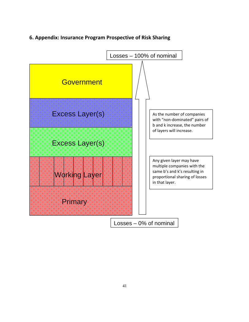
41

6. Appendix: Insurance Program Prospective of Risk Sharing

Excess Layer(s)

Excess Layer(s)

Government

Primary

Working Layer

As the number of companies with “non‐dominated” pairs of b and k increase, the number of layers will increase.

Any given layer may have multiple companies with the same b’s and k’s resulting in proportional sharing of losses in that layer.

Losses – 0% of nominal

Losses – 100% of nominal

42

7. REFERENCES

Albertini, L. and P. Barrieu, 2009: The Handbook of Insurance‐Linked Securities (New York, John Wiley & Sons), 398 pages.

Bauer, D. and G. Zanjani, 2011: “The Marginal Cost of Risk, Risk Measures, and Capital Allocation”, mimeo, Georgia State University.

Berger, L.A., J.D. Cummins and S. Tennyson, 1992: “Reinsurance and the Liability Crisis”, Journal of Risk and Uncertainty, 5:253–272.

Bernard, C. and W. Tian, 2009: “Optimal Reinsurance Arrangements under Tail Risk Measures”, Journal of Risk and Insurance, 76:709‐725.

Borch, K., 1962: “Equilibrium in a Reinsurance Market”, Econometrica, 30:424‐444.

Browne, M. and R.E. Hoyt, 2000: “The Demand for Flood Insurance: Empirical Evidence”, Journal of Risk and Uncertainty, v.20, no.3, pg. 291.

Cole C., P. Maroney, K. McCullough, J. Newman and C. Nyce, 2009: “A Review of the Development of Residual Market Mechanisms in Florida”, Journal of Insurance Regulation, 27 (4): 55‐80.

Cole C., D. MacPherson, P. Maroney, K. McCullough and C. Nyce, 2010: “The Use of Post‐Loss Financing of Catastrophic Risk”, Risk Management and Insurance Review, forthcoming.

Cummins, J.D., N.A. Doherty and A. Lo, 2002: “Can Insurers Pay for the Big One? Measuring the Capacity of the Insurance Market to Respond to Catastrophic Losses”, Journal of Banking and Finance, 26:557‐583.

Cummins, J.D., Lewis, C.M., Phillips, R.D., 1999: “Pricing excess of loss reinsurance contracts against catastrophic loss”, in K. Froot (Ed.), The Financing of Catastrophe Risk. The University of Chicago Press, Chicago.

Cummins, J.D. and P. Trainar, 2009: “Securitization, Insurance, and Reinsurance”, Journal of Risk and Insurance, 76:463‐492.

Cummins, J.D. and M.A. Weiss, 2009: “Convergence of Insurance and Financial Markets: Hybrid and Securitized Risk Transfer Solutions”, Journal of Risk and Insurance, 76:493‐545.

Dionne, G., R. Gagné, A. Nouira and J.D. Cummins, 2006: “Efficiency of Insurance Firms with Endogenous Risk Management and Financial Intermediation Activities”, Working Paper HEC Montréal CIRPÉE 06‐16.

43

Doherty, N.A. and S.M. Tinic, 1981: “Reinsurance under Conditions of Capital Market Equilibrium: A Note”, Journal of Finance, 36:949‐953.

Fazzari, S.M., R.G. Hubbard and B.C. Petersen, 1988: “Financing Constraints and Corporate Investment”, Brookings Papers in Economics, 1:141–195.

Froot, K.A., 2001: “The Market for Catastrophe Risk: A Clinical Examination”, Journal of Financial Economics, 60:529‐571.

Froot, K.A. and P.G.J. O'Connell, 1999: “The pricing of US catastrophe reinsurance”, in K. Froot, Editor, The Financing of Catastrophe Risk, Univ. of Chicago Press, Chicago, pp. 195–227. Froot, K.A. and P.G.J. O’Connell, 2008: “On the pricing of intermediated risks: Theory and application to catastrophe reinsurance”, Journal of Banking and Finance, 32:69–85.

Garven, J.R. and J. Lamm‐Tennant, 2003: “Optimality of a Stop‐Loss Reinsurance in Layers”, Insurance and Risk Management, 7:217‐237.

Harrington, S.E. and G. Niehaus, 2003: “Capital, Corporate Income Taxes, and Catastrophic Insurance”, Journal of Financial Intermediation, 12:365‐389.

Hartwig, R. and R. Wilkerson, 2007: “Residual Market Property Plans: From Markets of Last Resort to Markets of First Choice”, Insurance Information Institute.

Hartwig, R. and R. Wilkerson, 2010:“Update Residual Market Property Plans: From Markets of Last Resort to Markets of First Choice”, Insurance Information Institute.

Hurlimann, W., 2003: “Optimality of a Stop‐Loss Reinsurance in Layers”, ASTIN Colloquium International Actuarial Association – Brussels, Belgium.

Jaffe, D. and T. Russell, 1997: “Catastrophe insurance, capital markets, and uninsurable risks”, Journal of Risk and Insurance, 64: 205–230.

Jean‐Baptiste, E.L. and A.M. Santomero, 2000: “The Design of Private Reinsurance Contracts”, Journal of Financial Intermediation, 9:274‐297.

Kessler, D., 2008: “Insurance market mechanisms and government interventions”, Journal of Banking and Finance, 32: 4–14

Kleffner, A.E. and N.A. Doherty, 1996: “Costly Risk Bearing and the Supply of Catastrophic Insurance”, Journal of Risk and Insurance, 63:657‐671.

44

Kunreuther, H. and E. Michel‐Kerjan, 2009: At War with the Weather: Managing Large‐Scale Risks in a New Era of Catastrophes, MIT Press.

Lewis, C.M. and K.C. Murdock, 1996: “The Role of Government Contracts in Discretionary Reinsurance Markets for Natural Disasters“, Journal of Risk and Insurances, 63:567–597.

Ladoucette, S.A. and J.L. Teugels, 2006: “Analysis of Risk Measures for Reinsurance Layers”, Insurance Mathematics and Economics, 38:630‐639.

Mayers, D. and C.W. Smith, 1990: “On the Corporate Demand for Insurance: Evidence from the Reinsurance Market”, Journal of Business, 63:19‐40.

Michel‐Kerjan, E. and J.V. Wise, 2011: “The Risk of Ever‐Growing Disaster Relief Expectations”, Working Paper, The Wharton School of the University of Pennsylvania.

Modigliani, F. and M.H. Miller (1958): "The Cost of Capital, Corporation Finance, and the Theory of Investments," American Economic Review, 48: 261‐297.

Myers, S.C. and N.S. Majluf, 1984 : “Corporate Financing and Investment Decisions when Firms Have Information that Investors Do not Have”, Journal of Financial Economics, 13:187–221.

Niehaus, G., 2002: “The Allocation of Catastrophe Risk”, Journal of Banking and Finance, 26: 585‐596.

Niehaus, G. and S. Mann, 1992: “The trading of underwriting risk: a comparison of reinsurance and insurance futures contracts”, Journal of Risk and Insurance, 59: 601–627.

Nyce, C. and P. Maroney, 2011: “Are Territorial Rating Models Outdated in Residential Property Insurance Markets? Evidence from the Florida Property Insurance Market”, Risk Management and Insurance Review, 14: 201‐232.

Powers, M.R. and M. Shubik, 2001: “Toward a Theory of Reinsurance and Retrocession”, Insurance Mathematics and Economics, 29:271‐290.

Powell, L.S. and D.W. Sommer, 2007: “Internal Versus External Capital Markets in the Insurance Industry: The Role of Reinsurance”, Journal of Financial Services Research, 31:173‐188.

Sommer, D.W., 1996: “The Impact of Firm Risk on Property‐Liability Insurance Prices”, Journal of Risk and Insurance, 63: 501‐514

Tasche, D., 2004 : “Allocating Portfolio Economic Capital to Sub‐portfolios” In: Economic Capital: A Practitioner Guide, A. Dev (ed.). Risk Books, 2004, 275‐302.

45

Zanjani, G., 2002: “Pricing and Capital Allocation in Catastrophe Insurance”, Journal of Financial Economics, 65:283‐305.

Zanjani, G., 2010: “An Economic Approach to Capital Allocation”, Journal of Risk and Insurance, 77: 523‐549.

An Industrial Organization Theory of Risk Sharing

Documents

Transcript of An Industrial Organization Theory of Risk Sharing