Research Institute for Advanced Computer ScienceNASA Ames Research Center

An Improved Newton Iteration

for the Generalized Inverse of a Matrix,

with Applications

Victor Pan Robert Schreiber

1

RIACS Technical Report 90.16 March, 1990

To appear: SIAM Journal on Scientific and Statistical Computing

(NASA-CR-185983) AN IMPROVEO NEWTON

ITERATION FOR THE GENERALIZED INVERSE OF A

HAT£1X, WITH APPLICATIO'_S (Research Inst.

fOF Advanced Computer Science) 40 pCSCL 12A

G3/64

N92-I1723

Unclas004]049

https://ntrs.nasa.gov/search.jsp?R=19920002505 2018-05-07T15:35:46+00:00Z

An Improved Newton Iterationfor the Generalized Inverse of a Matrix,

with Applications

Victor Pan Robert Schreiber

1.4

U

0J

0.fl

O,4

0.2

02 0_ _ U 1 t.g _tA 1.6

The Research Institute of Advanced Computer Science is operated by Universities Space ResearchAssociation, The American City Building, Suite 311, Columbia, MD 244, (301)730-2656

Work reported herein was supported by the NAS Systems Division of NASA and DARPA via Cooperative

Agreement NCC 2°387 between NASA and the University Space P_esearch Association (USBA). Work wasperformed at the Research Institute for Advanced Computer Science (RIACS), NASA Ames Research Center,Moffett Field, CA 94035.

An Improved Newton Iteration for the Generalized Inverse of a Matrix,with Applications _"

Victor Pan

Computer Science Department, SUNYAlbany, NY 12222

and

Mathematics Department, Lehman CollegeCUNY, Bronx, NY 10468

(Supported by NSF Grant CCR-8805782 and PSC-CUNY Award 668541)and

Robert Schreiber

Research Institute for Advanced Computer ScienceMoffett Field, CA 94035

(Supported by ONR Contract number N00014-86-K-0610 andARO Grant DAAL03-86-K-0112 to the Rensselaer Polytechnic Institute,

and by the NAS Systems Division viaCooperative Agreement NCC2-387 between NASA and the

Universities Space Research Association.)

Abstract

Pan and Reif have shown that Newton iteration may be used to compute the inverse of an

nxn, weU-conditioned matrix in parallel time O(logha) and that this computation is processor

efficient. Since the algorithm essentially mounts to a sequence of matrix-matrix multiplications,

it can be implemented with great efficiency on systolic arrays and parallel computers.

Newton's method is expensive in terms of the arithmetic operation count. In this paper we

reduce the cost of Newton's method with several new acceleration procedures. We obtain a

speedup by a factor of two for arbitrary input matrices; for symmetric positive definite matrices,

the factor is four. We also show that the accelerated procedure is a form of Tchebychev accelera-

fion, while Newton's method uses instead a Neumann series approximation.

_e Submitted to the SIAM Journal on Scientific and Statistical Computing.

-2-

In addition, we develop Newton-like procedures for a number of important related prob-

lems. We show how to compute the nearest matrices of lower rank to a given matrix A, the gen-

eralized inverses of these nearby matrices, their ranks (as a function of their distances from A),

and projections onto subspaces spanned by singular vectors; such computations are important in

signal processing applications. Furthermore, we show that the numerical instability of Newton's

method when applied to a singular matrix is absent from these improved methods. Finally, we

show how to use these tools to devise new polylog time parallel algorithms for the singular value

decomposition.

Key Words: Matrix computation, Moore-Penrose generalized inverse, singular value

decomposition, Newton iteration.

Acknowledgements. We would like to thank the referees for many valuable suggestions,

especially for helping to simplify and clarify the proofs; Roland Freund and Youcef Saad for sug-

gesting the Tchebychev analysis; and Sally Goodall for expertly typing the manuscript.

1. Introduction

Pan and Reif [11], [12] have shown that Newton iteration may be used to compute the

inverse of an nxn, well-conditioned matrix in parallel time proportional to log2n using a number

of processors that is within a factor of log n of the optimum. Newton iteration is simple to

describe and to analyze, and is strongly numerically stable for no_ingular input matrices; this is

-3-

not true of earlier polylog time matrix inversion methods. Moreover, since it is rich in matrix-

matrix multiplications, it can be implemented with great efficiency on systolic arrays and parallel

computers. 1

Unforumately, the computation can be rather expensive. It has been shown that the number

of matrix multiplications required can be as high as 4 log k--(A), where k-'(A) .= I IA I 12 I 1A-t I 12.

Here we show how to reduce this cost, in some cases quite dramatically. We accelerate and

extend the usual Newton iteration in several ways. In particular, we

• substantiallyacceleratetheconvergenceoftheiteration;

• insure its stability even when A is singular;,

• show how to compute the matrix A(e) obtained from A by setting to zero any of its singular

values that are less than e. Thus A(e) is a closest lower rank approximation to A (see

Theorem 2.1 below);

• compute A+(e),the Moorc-Pcnrose generalizedinverse(alsocalledthepseudo-inverse)of

A(O;

• compute the rank of A(8);

I (On tl_ Connection Machine [7]matrixproductsmay be cornpute_lat5X10 9 Olm'ationsper second,but

matrix computations done in standardlanguagesrarelycan exceed I0 _ operationsper s_eontl.Furthermore,

computer manufacturersarectmrentlybeing encouraged toprovidethe f_mst numdx productsoftwarepossi-

ble,sinceothermatrixcomputations (QR and LU decomposition,inparticular)nmy be computed with algo-

rithmsthatarerichinmatrixmultiply[4].)

• compute the matrix P(e) that projects orthogonally onto the range of A(_).

Concerning acceleration, we obtain a twofold speedup by scaling the iterates at each step,

and we prove that the scaled iterates are defined by Tchebychev polynomials that are, in the usual

minimax sense, optimal in a subspace of polynomials in ATA. In the case of symmetric positive

definite matrices, we get another speedup by a factor of two through a new means of constructing

the initial iterate. We also consider adaptive procedures for which we prove no such a priori

lower bound on speedup, but which promise to be useful in practice. Our results have further

applications, in particular, to signal processing and to computing the SVD of a matrix.

Concerning efficiency in highly parallel computing environments, we do not claim that the

present methods are always advantageous. The alternative, for most computations discussed

here, is a parallel computation of the full SVD of A. The computation of the SVD in a highly

n n processors, implementing aparallel environment is best done using a square array of -2-x-2-

Jacobi-like method due to Kogbetliantz [3]. (This method is not competitive with standard

methods in terms of operation count, but the standard methods are not well suited to highly paral-

lel architectures). Good experimental evidence is available to show that from six to ten sweeps of

the Kogbetliantz method are needed. For real A, each sweep requires 8n 3 multiplications. The

sequential operation count of this method is therefore the same as that of 32 m 52 Newton itera-

tions. Thus, Newton's method is competitive with a Kogbetliantz SVD for these problems on

-5-

highly parallel computers. It is a clear winner if the condition number of A(e) is not too large, or

if the adaptive acceleration we employ is especially successful, so that far fewer than 30 Newton

steps axe needed, or if we can exploit sparsity or other properties of A to reduce its cost. Further-

more, it is often the case on parallel machines that matrix products, the core of the Newton item-

tion, can be computed especially fast. (On the Connection Machine, microeoded matrix multiply

rims an order of magnitude faster than code written in Fortran, C*, or *LISP.)

Of course, other parallel methods for the SVD may arise. And when the number of proces-

sors is not large, so that O(n 2) processors are not available, then more modestly parallel, but less

costly methods for the SVD are better.

I.I Contents.

We organize the paper as follows: Section 2 is for definitions. In Section 3, we recall the

customary Newton iteration for matrix inversion; in Section 4 we present a Tchebychev accelera-

tion procedure and in Section 5 an adaptive acceleration using cubic polynomials rather than the

quadratics used in Newton's method. We give a method for finding an improved initial iterate for

symmetric positive definite A in Section 6. In Sections 7-9 we give methods for computing the

matrices A(e) and A+(e) (see above), prove the stability of these computations, show how to find

subspaces spanned by singular vectors, and show some further applications. Some numerical

experiments are presented in Section 10.

-6- , ,

2. Notation

We denote most matrices by upper case Roman letters, diagonal matrices by upper case

Greek letters, and the elements of a matrix by the corresponding lower case Greek letter. We also

use lower case Greek letters for various scalars, lower case bold Roman letters for vectors and in

particular, columns of matrices. The letters i, j, k, m, n, r, and s are used for integers. We assume

that all the quantities are real; extension to the complex case is straightforward.

The basis for our analysis is the singular value decomposition (hereafter referred to as the

SVD) ofA e Rmxn,

A =UY-V r , (2.1)

where U=[ub "" ,urn] and V=[vl, "--,v,] are square orthogonal matrices and

Y_= diag(ol >-a2 _ "" • _ ar > ar+l = "'" = % = 0). Here, r = rank(A). The generalized inverse

of A is

where

A + = V]E+ U T

Y_+=_diag(oi -i,aE l, • • • ,Or 1,0, "" " ,0).

If A is symmetric and positive definite, then m = n and U = V. In this case, the eigenvalues

of A are c_jand the eigenvectors are vj, 1 < j < n.

We shall use the Euclidean vector norm I Ix I 12--E(xTx)1/2 and the following matrix norms:

IIA112 -ffimax_IIAx112/I Ix112

-7-

I IAI Ii mmax _,, laijl ,J l

I IAI I. --max _, Ior,ijl ,] j

L'J JIt is known [6] that if A has the SVD (2.1) then IIA112=oi, and

I IAI IF= I IZI IF=(_ioT) 1r2. The following theorem (the Eckata-Young Theorem) can be

found in [6]. p. 19.

Theorem 2.1. Let A be a matrix of rank r with SVD (2.1). Let s <_r be an integer, and let

Then

A, - ujojvjT .

IIA-A,112= rml_n=_ IIA-BI [2=a,+l .

Wc shallmake use,too,ofthespectralconditionnumber x(A) ofA, which isdcflncdby

x(A)E I IAI 12 IIA+112=al/O r. (2.2)

The chief reason for being interested in the generalized inverse is that the solution to the least

squares problem

mini IAx-bl 12

having smallest norm I Ix I 12 is A+b.

3. Newton iteration

Newton iteration

Xk+l ----Xk(2l - AXk) = (2I - XkA)X k (3.1)

was proposed by Schulz in 1933 for computing the inverse of a nonsingular matrix A [16]. Much

later,Ben-IsraelandCohen proved that the iteration converges m A + provided that

X 0 = tlt)A T,

with ao positive and sufficiently small [1], [2].

(3.2)

All the following discussion employs an SVD-based analysis of the method, first developed

by Soderstrom and Stewart [17], who observed that (2.1), (3.1) and (3.2) imply that each iterate

has an SVD of the form

X k= V._.kUT

with the matrices U and V of (2.1). The products XkA therefore satisfy

XkA = V RkV T

where Rk ---F-ky-m diag(pfk),p_k),... ,p_));moreover,forall1<j < n and allk _ 0,

(3.3)

1 - p_+l) = (p_)_ 1)2. (3.4)

Clearly, pjtO)= aoC2. For any Cto< 2/ai z, (3.4) implies the quadratic convergence of pj(k) tO one

for all j, 1 < j < r, and, therefore, of X k to A +. The optimum choice of oto in (3.2), which minim-

izes I I I - XoA I 12 by making prO)_ 1 = 1 - pr(°), is

2 (3.5)ao= a?+ar2.

Let _A) be given by (2.2). Then with the choice (3.5),

p(0)= 2I+ K(A)2'

so thatp(O)¢ I if r(A) islarge.

(3.6)

In practice, information about ¢_r is hard to get. We may instead

use a suboptimal but nevertheless safe altemative, such as

-9-

1 (3.7)fro= I IAIIxlIAII..'

Other choices ofoto which do not require an estimate of or are available [1], [2], [11], [12].

It follows from (3.4) that small singular values p_) approximately double at every step.

Therefore, it takes about 2 log2_A) steps of (3.1) to get to the point where pro`) > _A and an addi-

tional log log (l/c) iterations for convergence of all the pj to within E of 1. Thus, if the floating-

point operations are the measure of cost, the method is more expensive than the conventional

altematives. The mason for our interest in this method is that (3.1) essentially amounts to two

matrix multiplications, which can be very efficiently implemented on systolic arrays and on vec-

tor and parallel computers ([13], [14]). Further savings are possible: if A is sparse, then XkA is

less costly to compute; in the case of Toeplitz and many other structured matrices, AXk amounts

to a few matrix-vector products (see [8], [9], [10]). Finally, as only the product of A and some

vectors is required, we do not need to form A, which is convenient in some applications.

In operations counts, we use the term "flop" to mean a multiply-add pair. For unstructured

mxn matrices, each iteration step (3.1) essentially amounts to two matrix multiplications, that is

to 1.5mn 2 flops, exploiting the symmetry of AXk; in Section 5 we show how to reduce this to

about mn 2 + _hn 3 in a practical implementation.

4. Convergence Acceleration by Scaling

- 10- v.

Schreiber [14] presented the scaled iteration

Xk+l = (Xk+l(2I - XkA)Xk, k = 0, 1, .-. (4.1)

where Xo is given by (3.2). Here, we employ an acceleration parameter (Xk+le [1,2] chosen so as

to minimize a bound on the maximum distance of any nonzero singular value of Xk+lA from one.

Let us assume that we know bounds Ominand Omaxon the singular values of A satisfying

Or= --<02 --<O? Om. .

In this case, every eigenvalue of ATA lies in the interval [Omin,Omax]. (We assume this interval has

nonzero length; otherwise A is a scalar multiple of an orthogonal matrix and Xo is its inverse.)

We then choose Xo according to (3.2) with

2 (4.2)ff'O --- Omin + Omax "

It follows from (2.1), (3.2), (4.1) and (4.2) that for all j and k,

and

p jr0)_ 2°j2Omin + Omax '

To determine the acceleration parameters o_, for k > 0, we let

and

2or= (4.3)12(°)= o_r= = or= + _.,x

20mix . (4.4)_(0) = (XOOma x - Groin + Om_ '

these being lower and upper bounds on the singular values of XoA. Then take

-11-

Otk+l= _0¢+1)= 2l+(2-.O_O0)_&) '

which is both an acceleration parameter and an upper bound on {p_+_)}, and

(4.5)

p_&+1)= _+I (2--P_(k))P_&), (4.6)

which is a lower bound on {p_+0}. The definitions (4.3)-(4.6) imply that for all 1 <j < r and

k>l,

and

12(k)= 2 - _(k). (4.7)

(Note that (4.7) follows from immediately (4.5) and (4.6). The upper bound p_) < _00 is likewise

straightforward. Finally, if

then

(2--_O0)p_O0< (2-p_))p_) < 1,

whence, by (4.6) and the definition of pjt_) the lower bound fl00 < pjtk)fouows.)

Except for the last few iterations before convergence, 1200_ 1, which implies that ak+l = 2.

Thus, p_+l) = 4pr(k). Therefore,

- log4Pr(°)= log2[(_A)2+ I)I/2]= log2k'(A)+ O(I/_A) 2)

stepssufficeto bringallthe singularvaluesof XkA up to V2,which ishalfas many as forthe

unaccelerated version.

- 12- v

We shall now derive a theorem concerning the optimality of the acceleration parameters

given by 0.5). Let the symmetric residual matrix initially be

E - I - otoATA = I - XoA. (4.8)

It is straightforward to show that Newton's method, starting with Xo = otoAT, produces iterates Xk

satisfying

XkA = I -- Em (4.9)

where m = 2k. For a nonsingular matrix A and for the choice (4.2) for tXo, the eigenvalues of E lie

in the open interval (-1,1), and we have that E = _ 0 and, therefore, XkA _ I as k _ -0.

Furthermore, (4.8) and (4.9) imply that

Xk--(I+E + --- +Eat-l)_A T.

Thus, Newton's method is related to the Ncumann series expansion

(I-E) -1 = I + E + E2 + .. •

We therefore ask whether the accelerated method (3.2), (4.1) B (4.6) is related to a better

polynomial approximation to (I-E) -l. In fact, it is exactly equivalent to approximation of this

inverse by a Tchebychevpolynomial in E, as we now show.

Let

T2,(_ ) -- coS (2 k Cos-l_)

be the Tchebychev polynomial of degree 2 k on (-1,1). Recall that To(_) = 1, Tl(_) = _, and

T2,.,(_) =2 T],(_) - 1. (4.10)

- 13-

The scaled Tchebychev polynomials on (am_n,Om_ arc defined by

T2_(_ + 5)tk(_) -= T2,(8)

2 -(am_x + amin)where T = (Oma x _ Omin ) and 8 = (Oma x _ (I .rain ) .

tk(O) = 1, so that

Surely, tk is a polynomial of degree 2k, and

tk( ) = 1-- Tk( )

for some polynomial Y4,of degree 2k--l; furthermore, it is a classical result that among all such

polynomials, tk minimizes the norm _ s't_c_ ' [tk(_)l -ffiI I tkl I..(a..,a,.). They also satisfy a

recurrence like (4.10). Let [_k-=T2_(_). Then by (4.10),

[_ktk(_) ----2(_k-llk-1(_)) 2- I.

Theorem 4.1. Let the sequence of matricesXk, k=0, I, "'"

(4.6).Then

(4.11)

be generatedby (3.2),(4.1)--

Xk = [_k(ATA)A T

where _(_) is a polynomial of degree 2k---1.

polynomial tk(_) of degree 2 k on (Omin,Om_x).

(4.12)

The polynomial 1 - _ _(_) is the scaled Tchebychev

Remark. Before proving the theorem, we point out that (4.12) implies that

I - XkA = I - pk(ATA),

and therefore that

II I-XkA112=max I I--pk(O2)lI <j._n

which shows the relevance of the theorem's conclusion.

An analogue of this result also holds for Xo any matrix of the form r(ATA)A T, with r a poly-

nomial, such that the 2-norm of I - XoA is less than one.

Proof. The claim (4.12) is clearly true when k=0, with _(_) =ao. With the choice (4.2),

1 - _(_) = 1 - 2_ / (am_+C_m0 = to(X) is the appropriate scaled Tchebychev polynomial.

Now use induction on k. A straightforward calculation using (4.5) and (4.7) shows that, for

all k > 1, l<0_k<2 and _k = 1 _ It also follows from (4.1)----ZT- , or equivalently that _ =

and the inductive hypothesis in the form (4.12), after multiplying by A, that (4.12) holds for the

polynomial

=

From this and the relations between C_kand lBkwe derive the recurrence

_k(1 -- _) = 2_k2-1(1 -- _-l) 2 -- 1.

Thus, _(1 - _,) satisfies the Tchebychev recurrence (4.11), which proves the theorem.

QED

5. Convergence Acceleration with Cubic Polynomials

In Section 3 we saw that with the unaccelerated Newton method, the convergence of p_) to

one is slow for all j such that pit0) lies near zero or two. For many input matrices, and for

moderately large k, the set {pjfk)}jn,0 produced by Newton's method without acceleration consists

- 15-

of two clusters, one lying near zero and the other near one. In this section, we present an altema-

tive to the acceleration method of Section 4 that, in the case of such a large gap in the spectrum of

XkA, results in much faster convergence.

Let X be a fixed matrix satisfying XA = VRV T, R = diag(pl, • "" ,P,0 where 0 -<pj -<2 for

allj. We seek an improved approximation Xl to A + of the form

Xl -- (,y3(XA) 2 + Y2XA+TII)X.

We choose {)'1,Y2,)'3} so that the cubic polynomial c(p) =),fla + y2p 2 + ._p3 satisfies

(i) c(1)- 1,

(ii) c'(1) = 0,

(iii) c(0) = 0,

(iv) c'(O) :3, 2.

The idea here is that small singular values are amplified by the factor c'(0) while those near

one continue to converge. It is quite evident, however, that c(9) will take large values for some

p e (0,1), so we must exercise caution.

We begin by finding 12> 0 such that we are certain that there are no eigenvalues pj in

(_,1---_) or in (1-q2,2]. Let T=XA and compute T2 and 8- I IT-T21 IF. Now, it follows from

(3.3) that

2= _ [pj(l_p)]2;J(5.1)

whence, for _11 1 < j _<n,

-16-

pj II-pjl __.8.

If 8 _ ¼, this provides us with no useful information. If, on the contrary, 0 < 8 < ¼, then we con-

dude that all the eigenvalues pj lie in the two closed intervals: [O,p_]and [I -12,1 + p], where

and

O_<_m_-_-8<_,

V_< 1 -_ffi_+ V'_/_-8,

(See Figure I).

0.25

0.2

0.15

0.1

0.05

0

-0.05

-0.1

-0.15

-0.2

-0.250 0.2

Figu_ 1. The intarvals8= J IXA-(XA)21 IF< ¼.

Thus, forj = 1, .-- , n,

pj • [O,p.]u [1 -fi,1 +p].

0.4 0.6 0.8 I

[0,_ _d [I-_,I+p1 contain _ the pj when

(5.2)

8

-8

-17-

inotherwords pjisinneither(12,1-p.)nor (I-_,2].Now wc show how tochoose c(p)so asto

satisfy the criteria (i)-(iv), as well as the equally important criteria

(v) c:[0,p_]_ [0,I],

(vi) c:[I--_,I+p)---)[l,l+p_).

To determine c, we enforce (i)-(iii) together with

(vii) c(p_.)= 1.

The unique solution is

c(p)= _(p2 _ (2+p_)p

which may be rewritten as

+ (1+2p_))p,

c(p)= _((p-1) 3+ (1-p_)(p-l)2)+ I.

Theorem 5.1.Let 0 <.p_.<_'A.Ifc(p)istheuniquecubicsatisfying(i),(ii),(iii),and (vii)above,

then (v) and (vi) hold.

Proof: To show that (v) holds, we recall that a nonvanishing cubic polynomial c(p) has at most

two critical points (where c'(p) - 0). One of these is p = 1 (condition (ii)). By (i), (vii) and

RoUe's theorem,theotherone isin(_,I),so c(p)ismonotone on [0,p_..]and must thereforemap

[0,12] onto [0,1].

To establish (vi), note that

c(p)= 1+ (p- I)2(P_ P-).

-18- ...

Now let p= 1 -8 with lel_R<lt2. Then c(p)- 1 =¢2(1 - 8- P_)/fi, and since the second factor

is bounded by 0 and 1, the fight-hand side is bounded by 0 and gZ,establishing (vi).

QED

Thus, if 8 > IA we cannot accelerate. In this case, we let XI = (2I - T)X and proceed to the next

iteration (i.e., XI is the result of a Newton step (3.1)). On the other hand, if 5 < _Awe compute

:= _A- _ and let XI - _(T 2 - (2+p_)T + (l+2p_)I)X (i.e., Xl is the result of a cubic step).

-19-

Here is a practical algorithm incorporating this idea for computing A+.

ALGORITHM CUINV.INPUT: AOUTPUT: A +

STEP 0 [INITIALIZE]:

Choose X = ¢xoAT, wiuh ao given by (4.2) or (3.7);T :- XA;T2VALID := false;

STEP 1 [NEWTON STEP]:

if X is sufficiently close to A+ then return(X);X := (2I-T)X;if T2VALID then

T :- 2T-T2else

T := XA;endi____fT2VALID := false;

if trace(T)__n - tA then_oto STEP 1;

STEP 2 [TEST FOR SMALL CHANGE]:T2 := T2;

:= I IT-T21 IF;if _>¼ then

T2VALID := true;_oto STEP 1;

elseog.qLQSTEP 3;

STEP 3 [USE ACCELERATION]:_:=__ ,4_,_&

X := --_-(T2-(2+fl)T+(I+2R)I ) X;,i

T := XA;

_oto STEP 1;

COMMENTS on ALGORITHM CUINV.

(1) Stopping criteria are discussed by Soderstmm and Stewart [17].

(2) First, we have made use of the fact that after a Newton step (3.1),

Tk+I,=Xk+iA

= (2I-XkA)XkA

= (2I--Tk)Tk.

- 20 - ,..-

Thus, if we decide to reject the use of a cubic acceleration step, the computation of T 2 in

STEP 2 is not wasted, because it saves us at least that much work in the following Newton

step (STEP 1).

(3) We do not use cubic steps exclusively; we do need at least one Newton step for each cubic

step because without Newton steps, we cannot find intervals [0,p_] and [1 -g!,l +p..] known

to contain all the eigenvalues. Furthermore, the Newton steps finish the job of forcing

eigenvalues near one to actually converge.

(4) We use only Newton steps when all the singular values of XA are close to one. This is sig-

naled by the convergence of trace(XA) to within one half of its limiting value of n.

If A is an mxn matrix, then we assume that the cost of computing the product XA is _Amnz

flops (we exploit the symmetry of XA), the cost of computing the product "1̀2 is 1/2n3 flops, and the

cost of computing X in STEP 1 or STEP 3 is mn 2 flops. Then, if we skip STEP 3, an iteration of

CUINV costs

nZm + 'An3 flops,

assuming that T2VALID was true. The cost of an iteration in which we take STEPS 1 -- 3 is

3mn 2 + _An3,

assuming that T2VALID was false. These assumptions are warranted since it is the iterations that

take STEP 3 that cause T2VALID to be false. Thus, for n = m, we pay a premium of only about

16% compared with two Newton steps.

What is the effect of a full iteration assuming STEP 3 is taken? Formally, the eigenvalues

of XA are mapped as follows:

--->c((2---p)p)= I+I-_ (l---p)4- _-(l---P)6- C(p;p_). (5.3)P

For smallp, C(p;p_)= (4+_-)p. And becauseitwilloftenbe thecase thatp_¢: I,the combined

iterationgreatlyamplifiesthe small eigenvalues.Those nearone continueto converge super-

linearly;equation (5.3)shows that

I 1--C(p;p_) I = _ (i--p) 4 + o((1-p) 6)

-21 -

< (1--p_)(1--.p)3 + O((1--9) 6) = 0((1--t9)3).

since any eigenvalue p of XA exceeding fl must be in [1 - _,1 + p..], so R >_1-p.

See Section 10 for some experimental evidence of the efficiency and reliability of ALGO-

RITHM CUINV.

6. An Improved Initial Iterate in the Symmetric Positive Definite Case

Let us consider the case of a symmetric positive definite matrix A, which is important in

many applications [6]. Given a matrix A with the SVD

A=VZV T, Z=diag(ol> ... >on>0) (6.1)

(which is its eigendecomposition, too) we shall choose

Xo = 13I+ (xoA (6.2)

so as to optimally place the singular values of XoA. From (6.1) and (6.2)

XOA -" V(,_X + OtO_2)V T .

We choose ([3,O.o)so that, with p(a) -=15o + o_o 2, the largest possible initial error

III-X0AII2ffi max Ip(o)-llo._o_ot

is minimized.

on (%,O1):

By standard arguments (see [5], ch. 9), 1 -p is a scaled Tchebychev polynomial

where Omid m 1/2(% + Ol ) and _ - o I - Omid. Moreover,

III-XoA112= max IT2(o)I =T2(Ol)= _2o, _;o<o, 20_id - _2 "

We are most concerned about p(o) the smallest singular value of XoA, which is

p(On)- 2(Om2id- _2)

202mid _ _2

Let _ =/5/Omid < 1. The condition number 1¢is given by _:= ol/on. Thus

Omid "t'_ ] +(,0 .

Omid-- _i 1 -- (O '

1 - p(o) -- T2(O) ffi 2(0 - Omid) 2 -- _220_id -- _2

- 22 -

whence

to-1to=_.

Thus, the smallest initial singular value of XoA is

p(a.) - 2(1 -2 - 002

= 2(0( + 1) 2 - (K - 1) 2)

2(K + ! )2 _ (K - 1)2

1¢2+ 61¢+ 1

This asymptotically is 8x:-_ +O0¢-2), which is far larger than the 2K -2 provided

"optimal" choice Xo = txoA (see (3.6))! To find [3, ao, and hence Xo, we use the equations

[_ + a0a 2 = p(o) = 1 - T2(¢_)

20_id - 52 - 2(0 - (_mid)2 + q_2

2o&d-

-2a 2 + 4_amid

-r9

Hence

(6.3)

by the

4{_mid . 2

_ 2a_a - 82' ao E-- 2a_a - 52 " (6.4)

Remark. Even without computing estimates or bounds for the extreme singular values we

may improve the initial approximation when A is symmetric positive definite by choosing

Xo=(1/It A I IF)I; forin this case II I-XoA 112-< 1- 1/(ntrhc).

7. Suppressing the Smaller Singular Values

In this section, given a matrix A and a positive scalar ¢, we show how to compute A(e) and

A+(e) , where A(e) is obtained from A by suppressing (that is, setting to zero) all the singular

values of A that do not exceed e. (As noted in Section 2 above, A(e) is a closest approximation

to A by matrices whose rank is that of A(e). In practice, solving least squares problems often

requires the use of this form of regularization; for when A is very badly conditioned, its general-

ized inverse is largely unknowable due to perturbations in A, but the reduced-rank generalized

inverses are much better conditioned. This idea is discussed more fully by Golub and Van Loan

-23 -

[6,Section5.5].)

In ordertocompute theserank-reducedgeneralizedinverses,we requirea polynomialc(p)

that gives fast convergence to 0 near p = 0 and to 1 near p = 1. Consider first the iteration

Xk+l/2 = (2I-XkA)Xk, Xk+l -" Xk+l/2 AXk+lf2 (7.1)

that was proposed by the second author [14]. The eigenvalucs of XkA satisfy the equations

p_+l)= ((2..pj_k))p_))2forallj and k. Figure2 illustratestheeffectof thismapping. The fixed

poi_,arc_o=0,_,=(3--_)/2=.3s19...._2=I,and_3=(3+_)_=2.61S...which

aretherootsofthequartic(2_)2_2= _.1 ! i | !

2

Evidently, the

{P:Pl < P < 2-'pI}; note that

eigcnvalues from the former interval are sent

towards zero and from the latter interval towards one. The convergence is ultimately quadratic

but is slow near [_! and 2--pi. To compute A+(_), it suffices to apply the iteration (4.1) -- (4.6)

with appropriate omm and Om.x until the following relations hold:

3

- 24 -_'.

0 < p_) < 91 if and only ifoj < e,

t_l < pj_) < 2-_1 otherwise.

We can satisfy (7.2) for k = 0 by setting

proceed as follows:

(7.2)

(7.3)

tXo= 91 / e2, but then (7.3) may not hold. Therefore, we

0) Compute an upper hound Om_ on ol2.

1) Set oo = rain{2 / (Om_ + e2), 151/ e2}. This insures that the eigenvalues pjtO) (of XoA)

corresponding to the singular values oj > e (of A) are all closer to one than the smaller

eigenvalues. Set 5 (0) = o.0Om_, 12(°) = t_ 2.

2) Apply the iteration (4.1) with parameters given by (4.5) and (4.6) until 1200> 91.

.>.tx.[4) Apply the iteration (7.1) until the matrix A+(e) has been computed with the desired

accuracy.

The scaling at Step (3) is done to insure that all the small singular values 0ess than e ) are in fact

suppressed.

The iteration (7.1) associated with the quartic polynomial (9(2-9)) 2 is not the most efficient

way of computing A+(e). The same objective can be achieved by using the iteration

X (k+t) - (--2X(k)A+3I)X(k)AX(k) (7.4)

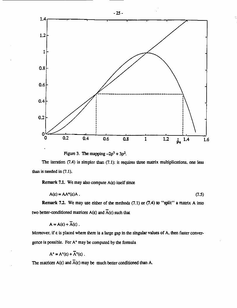
associated with the cubic polynomial e(p)=-2p3+3p 2 (see Figure 3). Note that e(1)= 1,

e(0) = e'(0) = e'(1) = 0, e(1/2) = 1/2, so that the mapping e(p) has three nonnegative fixed points

0, 1/2 and 1. Let 94 = (1+'f3)/2 = 1.366 .-. be the unique solution to -29,{ + 3t_,_ = 1/2 greater

than one. The eigenvalues of Xtk)A in the interval {p: 0 < p < 1/2} are sent towards zero, and the

eigenvalues in the interval {p: 1/2 < p _<1_4} are sent towards one; the convergence to zero and

one is ultimately quadratic but is slow near 1/2 and 1_4.

=25=

!

00 0.2 0.4 0.6 0.8 1 1.2 1.6

Figure 3. The mapping -2p 3 + 3p 2.

The iteration (7.4) is simpler than (7.1): it requires three matrix multiplications, one less

than is needed in (7.1).

Remark 7.1. We may also compute A(£) itself since

A(e) = AA÷(e)A. (7.5)

Remark 7.2. We may use either of the methods (7.1) or (7.4) to "split" a matrix A into

two better-conditioned matrices A(e) and A(e) such that

A = A(O + X(_).

Moreover, if £ is placed where there is a large gap in the singular values of A, then faster conver-

gence is possible, For A+ may be computed by the formula

A +ffiA+((_)+ X+((_).

The matricesA(8)and A(8) may bc much betterconditionedthanA.

8. Stability of the Basic and Modified Iterations

It is well-known that Newton iteration (3.1) is numerically stable and even self-correcting if

the input matrix A is nonsingular. If A is singular, however, then it is very mildly unstable.

and

Let A and A+ have the SVDs

A' v[0 IUTIn order to analyze the propagation of errors by (3.1), we assume that

[_'+ E,, El2]

Xk=A++ =Vlwhere 1_= VEU r is the current error in Xk.

tion amplifies these errors. Throughout this section we shall drop all terms of second order in E.

u T" (8.1)

We shall consider whether or not the Newton itera-

Using (8.1) it is simple to compute that

Xk+l =Xk+O-XkA)Xk

Due to the block 2E_, the iteration (3.1) is mildly unstable if A is singular (in which case the

(2,2) block above is not empty). After 21og2_A) iterations, rounding errors of order _(A) can

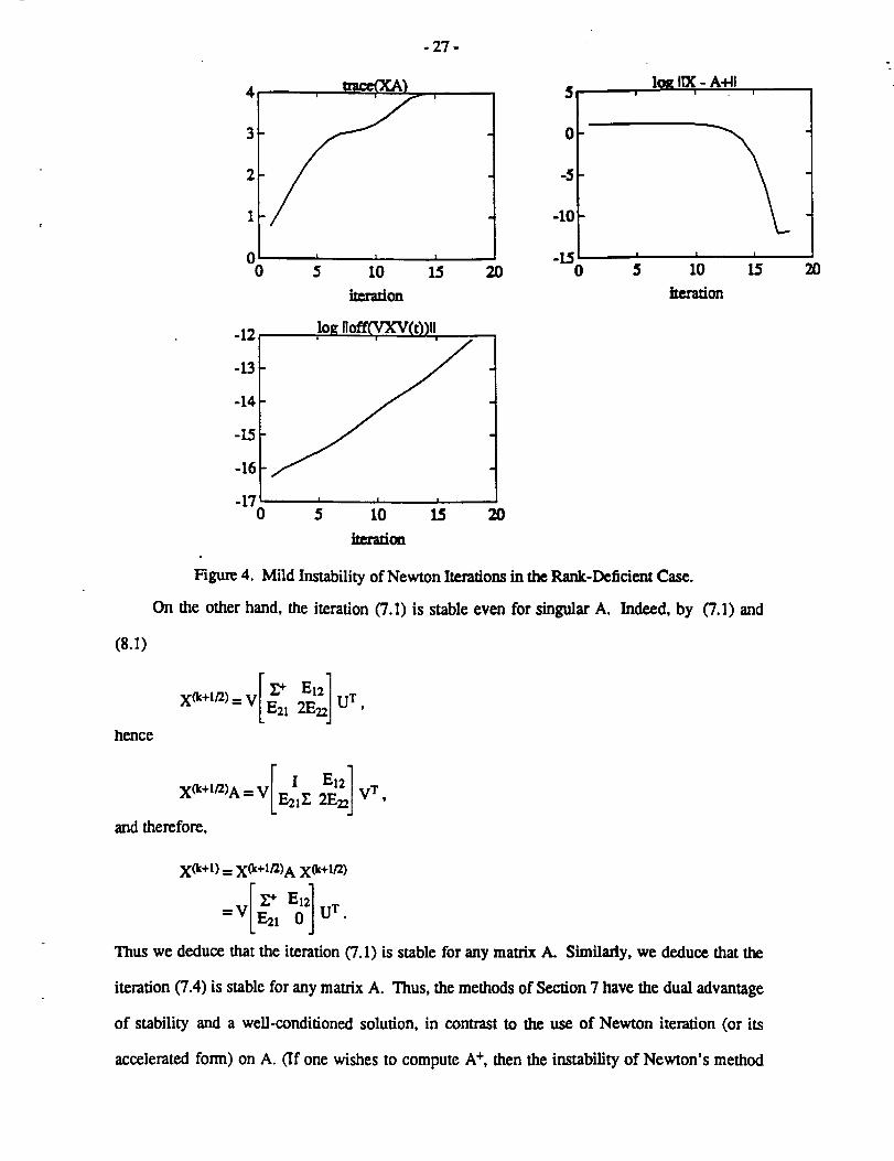
accumulate. In Figure 4, this phenomenon is illustrated. Here, A was 6x6 with condition number

30 and rank four. The method converges in 17 iterations. All logarithms are base 10 and the Fro-

benius norm is used. Note that the norm of the off-diagonal part of VXV T grows exponentially. It

reaches a value about four orders of magnitude above machine precision (which is roughly

10-16); a loss of four digits of precision results.

- 27 -

4

3

2

I

00

i

r _, , I5 10 15

5

0

-5

-I0

-150

|oI_ IIX - A_Ii

i I

10 15

tte_'afion

-12

-13 _

-14

-15

-16

tog ,oe

/

-17 ' ' '0 5 10 15 7.0

Figure 4. Mild Instability of Newton Iterations in the Rank-Deficient Case.

On the other hand, the iteration (7.1) is stable even for singular A. Indeed, by (7.1) and

(8.1)

V _x(k+l/2)-- [E21 2_] uT,

hence

E12] vT 'X(k+'t2)A=V Eli:

and therefore,

20

X(k+D -- X(k+It2)A x(k+I/2)

Thus we deduce that the iteration (7.1) is stable for any matrix A. Similarly, we deduce that the

iteration (7.4) is stable for any matrix A. Thus, the methods of Section 7 have the dual advantage

of stability and a well-conditioned solution, in contrast to the use of Newton iteration (or its

accelerated form) on A. (If one wishes to compute A +, then the instability of Newton's method

-28 - .

can be partly removed by using a few iterations (7.1) or (7.4) after all the significant singular

values have converged. Some practical details of this technique are discussed in Section 10.)

9. Computing the Projection onto a Subspaee Spanned by Singular Vectors

In this section we discuss a modification of the Newton iterations discussed above that

allows us to compute the orthogonal projection matrices onto subspaces spanned by the singular

vectors corresponding to either the dominant or the smallest singular values at less expense than

computing the generalized inverse of A. Important applications to spectral estimation and direc-

tion finding with antenna arrays were developed by Schmidt [15].

Let us define the matrices

p(_) = AA+(e)= U[A _] U T (9.1)

and

I 0_] vT (9.2)P'(I_) = A+(e)A = V 0

where the matrices U and V are from (2.1), I is the r(¢)xr(e) identity block, and r(e) is the number

of the singular values of A that are not less than _. Then P(e) and P'(e) are the orthogonal projec-

tions onto the subs'paces spanned by the first r(e) columns of the matrices U and V, respectively.

Our previous results already give us some iterative algorithms for computing

A(e) = (A+(e)) += AA(e)+A, as well as P(e) and P'(e), but there are simpler and more efficient

algorithms that we shall give shortly. In addition to the signal processing application mentioned

above, we may use this technique as an alternative to the methods of Section 7 for computing

A(e), since

A(e) = P(e)A = AP*(e). (9.3)

The following iteration extends (7.4) and converges to P(e), unless e is a singular value of

A. Let

Po = ff_ -AT + 13I, (9.4)

where we choose ao > 0, 13---0, to satisfy

-29 -

o_ 2 + _- 1/2; _ + _ < P4--- 1.37 -'- . (9.5)

then iterate as follows:

Pk+l --(--2Pk+31)Pk2= (I-2(Pk--l))Pk2 k-0, I, ''' (9.6)

The convergenceofPk toP(_)immediatelyfollowsfrom theconsiderationsofSection7.

The iteration(9.4)-(9.6)convergesto P*(_:)ifwe replaceAA T by ATA in (9.4).Further-

more, we may compute A(e) by using(9.3),which issuperiortothe solutiongiven inSection7

becausewe now need to compute a singlegeneralizedinverse(ratherthantwo). Also,each itera-

tionstep(9.6)only involvestwo matrixmultiplications.And finally,ifA isrectangularthenone

of theseiterationsislessexpensivethan (7.4)(forexample) because itinvolvessmallersym-

metricmatrices.

Remark 9.1. The stability analysis of Section 8 can be immediately extended to the itera-

tion (9.6).

1.5

0.5

0

I I .e" j|-" _ s o,p

r

; -* so

, ap+p ,.,-" i ..'"i # , ••

•- .a" • w-

........................................................i....................,,:."..... _•°..................................

: .°

.°

• /° _ •

o•• ,.° • _.,0 .," :

• • .s •

,o• .' • ...

"_ / , i i

o••• ,p's" ;-"

d " d"_' .... I i

0 0.5 1 1.5

Figure 5. Acceleration by scaling and shifting, P := aP + {]I.

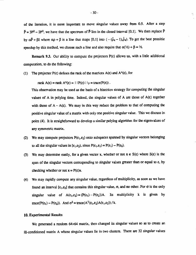
Remark 9.2. We may accelerate the cubic iteration for P(e) as follows. At the early stages

- 30- .:.

of the iteration, it is more important to move singular values away from 0.5. After a step

g) = 3P2 - 2P 3, we have that the specmun off lies in the closed interval [0,1]. We then replace

by ct_ + 13Iwhere ctO+ _ is a line that maps [0,1] into ( - _4 - 1),p4). To get the best possible

speedup by this method, we choose such a line and also require that o(IA) + i_= l/t2.

Remark 9.3. Our ability to compute the projectors P(8) allows us, with a little additional

computation, to do the following:

(1) The projector P(e) defines the rank of the matrices A(e) and A+(e), for

rank A(e) = rank A+(8) = I IP(e) I IF = trace(P(e)).

This observation may be used as the basis of a bisection strategy for computing the singular

values of A in polylog time. Indeed, the singular values of A are those of A(e) together

with those of A - A(8). We may in this way reduce the problem to that of computing the

positive singular value of a matrix with only one positive singular value. This we discuss in

point (4). It is straightforward to develop a similar polylog algorithm for the eigenvalues of

any symmetric matrix.

(2) We may compute projectors P(el,e2) onto subspaces spanned by singular vectors belonging

to all the singular values in [el,e2), since P(el,82) = P(EI) - P(Sz).

(3) We may determine easily, for a given vector x, whether or not x • S(e) where S(e) is the

span of the singular vectors corresponding to singular values greater than or equal to e, by

checking whether or not x = P(e)x.

(4) We may rapidly compute any singular value, regardless of multiplicity, as soon as we have

found an interval [e_,e2] that contains this singular value, o, and no other. For 0 is the only

singular value of A(sbe2)=(P(80-P(82))A. Its multiplicity k is given by

trace(P(el) - P(ez)). And 02 = trace(AT(cl,e2)A(¢be2)) / k.

10. Experimental Results

We generated a random 64x64 matrix, then changed its singular values so as to create an

in-conditioned man'ix A whose singular values lie in two clusters. There are 32 singular values

-31 -

in the interval [1, 7.6] and 32 others in the interval [10-7,10-6].

iter trace(XA)0 8.6801e-011 1.6882e+002 3.1987e+003 5.7784e+00

4 9.6436e+005 1.4398e+016 1.9113e+017 2.3340e+018 2.7108e+01

9 3.0015e+0110 3.2111e+0111 3.2003e+0112 3.2014e+0113 3.5992e+01

14 3.8974e+0115 4.3075e+0116 4.7663e+0117 5.2046e+0118 5.5954e+01

19 5.9225e+0120 6.1749e+0121 6.3309e+0122 6.3906e+0123 6.3997e+0124 6.4000e+0125 6.4000e+01

I IXA-II I

1.0000e+00

1.0000e+001.0000e+001.0000e+001.00(K_+001.0000e+00

1.0000e+001.0000e+001.0000e+001.0000e+001.0000e+001.0000e+009.9998e-019.9357e-019.8718e-019.7452e-01

9.4970e-019.0192e-018.1346e-016.6172e-014.3787e-011.9173e-013.6761e-021.3514e-03

1.8267e-067.6424e-09

12000000

00002.0481e-013.0331 e-038.4572e-067.0355e-0300

0000000000

Table 1: Results for First Test Matrix

We used algorithm CUINV to compute A-I. The initial iterate was that of (3.2) and (3.7). The

results are shown in Figure 6; the data are in Table 1, which gives lrace(XkA), I IXkA - I I 12, and

the computed bound 12 for k=0,1, ... ,12. Where _=0 the algorithm skipped the cubic

acceleration step. Early on this is because fi is too large, as the first 32 large singular values con-

verge. By way of comparison, Newton's method takes 60 iterations to obtain the solution pro-

duced by CUINV in 25.

- 32 -

uace(XA) leg IIXA - HI70 , , 0

6O

5oi

40

3O

2O

10

-1

" ! I,

10 20

-2

-3

-4J

-6_

-7

-8

"9 ! |

0 30 0 10 20 30

iteration

Figure 6. Convergence history for first test problem.

Next, we repeated this experiment with a second random matrix of order 64, having all its

singular values in [0.066, 1]. The method chose unaccelerated Newton steps (19 are required)

every time. Cubic steps were never used; this was due to the absence of any gap in spectrum of

XkA.

We therefore modified the algorithm so that when cubic acceleration is ruled out it uses a

step of adaptive Tchebychev acceleration as discussed in Section 4. For the practical application

of this idea. we require a means of finding a bound p,>O such that prO')<p,. We then use as the

acceleration parameter

2_k ffi l+(2-p.)p. "

This insures that the acceleration process does not cause a large singular value to be mapped to

the left of the smallest, thereby making the problem more difficult. Assume that the test 8 < _Aat

STEP 2 of CUINV fails. Let

-33 -

._=_/_.

Then, if _ < IA, we take

p. = IA_ 1_--_-_8

Now, since (5.1) holds,

mjn (pj - p_) < _.1 <:j _;n

Now it must be the case that Pr (the smallest positive singular value of XkA ) is less than p, or else

all of the singular values are in (1 - p., 1]. To rule out the latter possibility, we check whether

trace(XkA)_ n (I- p.)

and,ifnot,we accelerate.

With thischangc,thenumber of iterationsrequiredforconvergencedropped to 13 forthis

problem;thcoperationcountwentfrom 20.5c6to 14.6c6.

Evidently,even forwell-conditionedmatrices,modifiedCUINV can be farmore cfficicnt

thanNewton's method; formodcratclyiU-conditioncdmatrices,thedifferencesarcpmnounccd.

Next,wc generateda random 64x64 matrix,thenchanged itssingularvaluesso astocreate

an ill-conditionedmatrixA with 54 singularvaluesin [10-m,10-ll]and the remaining I0 in

[0.01,l].Wc computed thegeneralizedinverseof A(l.c-10),thematrixoftank 10 obtainedby

suppressingthe small singularvaluesof A. Wc firstused algorithmCUINV with A, choosing

ao= I. In additionwe monitoredthe growth of_ which was initiallysetequaltoe_10 "2°and

which isupdatedaccordingtotherccursions:

E := (2 - t:'-)_"

in Step 1 and

_:= _(_- (2 + p_)_+ (1 + 2p_))_

inStep3. Thus,e separatesthcsingularvaluesof XA thatwe wish to suppressfrom thosethat

we wish to map to one. At the first iteration in which the parameter 12,computed in Step 3, is less

than _, we stop and switch to the iteration (7.4) for, since (5.2) holds, the unwanted singular

values of XA must now be smaller than _A. In this example, the switch occurred after the seven-

teenth iteration. Table 2 gives the results; see also Figure 7.

12

10

6

4

2

00

-34-

_)| i !

! • | I

5 I0 15 20

0

-2

-4

-6

-8

-I0

"1,2 i , I I

0 $ I0 15

iteration iltzatioli

Figure 7. Convergence history for second test problem.

2O

iter tra_(XA)

1 3.9667e-01

2 7.2843e-013 1.2410e+00

4 1.8730e+005 2A361e+006 2.8749e+007 4.5728e+008 5.3217e+00

9 6.0588e+0010 6.7139e+0011 7.3764e+00

12 8.1084e+0013 8.7958e+0014 9.3559e+00

15 1.0110e+0116 1.000Be+0117 1.0000e+01

18 1.(X)0(O_I19 1.00(_+01

iIXA(£) - A(e)+A II

9.9997e-019.9995e-01

9.9989e-019.9978e-01

9.9957e-019.9913e-019.9271e-019.8548e-019.7117e-01

9.4318e-018.8958e-017.9136e-01

6.2625e-013.9219e-019.2682e-028.4375e-03

7.1182e-053.0452e-11

3.0452e- 11

1.0000e-20

2.0000e-204.0000e-20

8.0000e-201.6000e-193.2000e-192.6999e-185.3998e-181.0800e-17

2.1599e-174.3198e-17

8.6396e-171.7279e-153.4558e-165.3991e-15

1.2779e-123.5906e-08

o

0

00

0004.5074e-01

0000

0001.7207e-01

8.5950e-037.1192e-05

Table 2: Computing A(_:)+

The computed generalizedinverseisaccuratetoabout 11 digits.This issomewhat fewerthanwe

- 35 -

could wish, given that the condition number of this problem was 100. The loss of accuracy is due

to the fact that the accelerated Newton process (CUINV) went "too far", (raising e by 12 orders

of magnitude) before detecting the possibility of switching to the stable procedure (7.4).

11. Discussion

It has been our purpose here to clarify and illustrate the potential for the use of variants of

Newton's method to solve problems of practical interest on highly parallel computers. We have

shown how to accelerate the method substantially. We have shown how to modify it to success-

fully cope with in-conditioned matrices. We have developed practical implementations. We con-

elude that Newton's method can be of value for some interesting computations, especially in

parallel and other computing environments in which matrix products are especially easy to work

with.

References

[1]

[2]

[3]

[4]

[5]

[6]

U]

[8]

[9]

[I0]

A. Ben-Israel,"A Note on IterativeMethod for GeneralizedInversion of

Matrices,"Math. Computation,vol.20,pp.439-440,1966.

A. Bcn-lsracland D. Cohen, "On IterativeComputation of Generalized

Inversesand AssociatedProjections,"SIAM J.on NumericalAnalysis,vol.3,

pp.410-419,1966.

R.P. Brent,F.T.Luk and C. Van Loan, "Computation of the SingularValue

Decomposition Using Mesh-Connected Processors,"Journal of VLSI Com-

puterSystems,vol.1,pp.242-270,1985.

J.Dongarra,J.DuCroz, I.Duff,and S.Hammarling, "A Set of Level 3 Basic

LinearAlgebra Subprograms," ANL-MCS-P88-1, Argonne NationalLabora-

tory,Argonne,Illinois,1988.

D.K. Faddeev and V.N. Faddccva,ComputationalMethods oflu'nearAlgebra,

W.H. Freeman, San Francisco,1963.

G.H. Golub and C.F.van Loan, Matrix Computations,Johns Hopkins Univer-

sityPress,Baltimore,Maryland,Second edition,1989.

W. D. Hillis,The ConnectionMachine, Mrr Press,Cambridgc,Massachusetts,

1985.

V. Pan, "Fast and Efficient Parallel Inversion of Toeplitz and Block Toeplitz

Matrices," TR 88-8, Computer Science Dept., SUNY Albany, Albany, N.Y.,

1988.

V. Pan, "New Effective Methods for Computations with Structured

Matrices," Technical Report 88-28, Computer Science Dept., SUNY Albany,

1988.

V. Pan, "A New Acceleration of the Hilbert-Vandermonde Matrix Computa-

tions by Their Reduction to Hankel-Toeplitz Computations," Tech. Rep. TR

[11]

[12]

[13]

[14]

[15]

[16]

[17]

- 37 -

88-34, Computer Science Dept., SUNY Albany, Albany, NY, 1988.

V. Pan and J. Reif, "Efficient Parallel Solution of Linear Systems," Proc. 17-

th Ann. ACM Symp. on Theory of Computing, pp. 143-152, 1985.

V. Pan and J. Reif, "Fast and Efficient Parallel Solution of Dense Linear Sys-

tems," to appear in Computers & Math (with Applicau'ons), 1989.

M.J. Quinn, Designing Efficient Algorithms for Parallel Computers, McGraw-

Hill, New York, 1987.

R. Schreiber, Computing Generalized Inverses and Eigenvalues of Symmetric

Matrices Using Systolic Arrays, Computing Methods in Applied Science and

Engineering, R. Glowinski and J.-L. Lions, editors, North Holland, Amster-

dam, 1984.

R. O. Schmidt, "Multiple Emitter Location and Signal Parameter Estima-

tion," IEEE Transactions on Antennas and Propagation, vol. 34, pp. 276-280,

1986.

G. Schultz, "Iterative Bereclmung tier Rezipmken Matrix," Z. Angew. Math.

Mech., vol. 13, pp. 57-59, 1933.

Torsten Soderstrom and G. W. Stewart, "On the Numerical Properties of an

Iterative Method for Computing the Moore-Penmse Generalized Inverse,"

SIAMJ. Numer. Anal., vol. 11, pp. 61-74, 1974.