AN IMPROVED KRYLOV EIGENVALUE STRATEGY USING THE … · AN IMPROVED KRYLOV EIGENVALUE STRATEGY...

AN IMPROVED KRYLOV EIGENVALUE STRATEGY USING THEFEAST ALGORITHM WITH INEXACT SYSTEM SOLVES

BRENDAN GAVIN∗ AND ERIC POLIZZI∗

Abstract. The FEAST eigenvalue algorithm is a subspace iteration algorithm that uses contourintegration in the complex plane to obtain the eigenvectors of a matrix for the eigenvalues that arelocated in any user-defined search interval. By computing small numbers of eigenvalues in specificregions of the complex plane, FEAST is able to naturally parallelize the solution of eigenvalueproblems by solving for multiple eigenpairs simultaneously. The traditional FEAST algorithm isimplemented by directly solving collections of shifted linear systems of equations; in this paper, wedescribe a variation of the FEAST algorithm that uses iterative Krylov subspace algorithms forsolving the shifted linear systems inexactly. We show that this iterative FEAST algorithm (which wecall IFEAST) is mathematically equivalent to a block Krylov subspace method for solving eigenvalueproblems. By using Krylov subspaces indirectly through solving shifted linear systems, rather thandirectly for projecting the eigenvalue problem, IFEAST is able to solve eigenvalue problems usingvery large dimension Krylov subspaces, without ever having to store a basis for those subspaces.IFEAST thus combines the flexibility and power of Krylov methods, requiring only matrix-vectormultiplication for solving eigenvalue problems, with the natural parallelism of the traditional FEASTalgorithm. We discuss the relationship between IFEAST and more traditional Krylov methods, andprovide numerical examples illustrating its behavior.

Key words. FEAST, contour integration, eigenvalue problem, Kryov, Arnoldi, linear system

AMS subject classifications. 65F15,65F10,15A18

1. Introduction. Eigenvalue problems are a staple of basic linear algebra [8, 22],and they underlie a wide variety of practical computing techniques. Of particularinterest are problems such as ground state quantum chemistry, linear time-dependentsystems, and dimensionality reduction for data sets.

Conventional algorithms for small dimension eigenvalue problems (such as QRiterations) are generally unable to cope with the computational demands of the largerproblem sizes found in modern applications. Iterative algorithms that are designedspecifically for approximating the solutions to large eigenvalue problems, such asKrylov subspace methods (e.g. Lanczos and Arnoldi), tend to fare much better,and these are the primary methods that are used in solving the largest eigenvalueproblems in contemporary research. These methods, however, are not necessarily themost appropriate ones for modern computing architectures, particularly as scientificcomputing continues to approach the exascale. Modern high performance computingarchitectures achieve their promise of high performance through immense parallelism;Krylov subspace methods, on the other hand, are inherently serial algorithms thathappen to be able to benefit from having large amounts of memory available. Al-though they can be implemented and run on parallel computers, they are not ableto take full advantage of parallelism by actually dividing the task at hand into acollection of smaller, independent problems.

The likely best way forward for solving eigenvalue problems on modern paral-lel computing architectures is to use spectral slicing along with filtering techniquesin order to divide the spectrum of a matrix into an arbitrary number of smaller,non-intersecting regions in the complex plane. The eigenvalues (and correspondingeigenvectors) in each region can be filtered from the original problem and then solvedindependently of those in the other regions. As a result, one can solve for a large

∗University of Massachusetts Amherst Department of Electrical and Computer Engineering([email protected], [email protected])

1

arX

iv:1

706.

0069

2v1

[m

ath.

NA

] 2

Jun

201

7

mailto:[email protected]

mailto:[email protected]

2 BRENDAN GAVIN AND ERIC POLIZZI

number of eigenvalue/eigenvector pairs in a genuinely parallel fashion.In this paper we discuss a modification of the FEAST algorithm (which is an

example of a spectral filtering technique) that allows one to solve eigenvalue problemsfor large numbers of eigenvalue/eigenvector pairs by using only matrix-vector multi-plication, in order to provide a robust and naturally parallel alternative to traditionalKrylov iterative methods for the eigenvalue problem. We show that this modifiedFEAST algorithm, which we call Iterative FEAST (IFEAST), converges linearly tothe desired eigenpairs anywhere in the spectrum, and that it is mathematically equiv-alent to a restarted Krylov subspace method. Unlike other restarted Krylov subspaceeigenvalue algorithms, however, IFEAST provides a clear condition for convergencewhen restarting, and it can be implemented without having to store a basis for theKrylov subspace.

1.1. The FEAST Algorithm. FEAST [18, 25] uses a spectral filtering tech-nique that can select the eigenpairs of interest by using an approximate spectralprojector combined with a subspace iteration procedure. It can be used to solve thegeneralized eigenvalue problem

(1) AXI = BXIΛI ,

with

(2) A,B ∈ Cn×n, XI = {x1, . . . , xm}n×m, ΛI = diag(λ1, · · ·λm),

by finding all the m eigenvectors xi whose eigenvalues λi lie in some user-definedregion in the complex plane. For the sake of simplicity we consider only regionsthat are intervals I = (λmin, λmax) on the real number line, thereby restricting ourattention to Hermitian matrices. In general, though, FEAST, and all of the resultsin this paper, can be extended to non-Hermitian matrices as well [24, 12]. We alsorestrict our attention primarily to the standard eigenvalue problem case (i.e. B = I);the reasons for this will be addressed in Section 2.2.

FEAST selects the eigenvalues to solve for by using an approximation for thespectral projector ρ(A) = XIX

TI in order to form a subspace Q from a (possibly

random) initial guess for the eigenvectors X, thus guaranteeing that the columns ofQ span only the eigenvectors of interest. Because XI is unknown before solving theeigenvalue problem, FEAST uses complex contour integration in order to form anoperator that is equal to ρ(A):

Q = ρ(A)X = (XIXTI )X =

1

2πi

∮C(zI −A)−1Xdz.(3)

This integral can not be evaluated exactly; in practice, multiplication by ρ(A) isevaluated approximately by using a quadrature rule:

ρ(A)X =1

2πi

∮C(zI −A)−1Xdz(4)

≈nc∑k=1

ωk(zkI −A)−1X ≡ ρ(A)X(5)

The spectral projector is thus applied in an approximate way to the estimated sub-space X by solving nc shifted linear systems, and adding their solutions together in

IFEAST: AN OUTER-INNER ITERATIVE STRATEGY FOR THE FEAST EIGENSOLVER 3

a weighted sum. Thereafter, the original eigenvalue problem is solved approximatelyin the subspace spanned by Q by using the Rayleigh-Ritz procedure, giving new esti-mates of the desired eigenvalues and and eigenvectors. The estimated eigenvectors andeigenvalues are improved iteratively by repeating this procedure until convergence.

FEAST can be interpreted as a subspace iteration that uses the approximatespectral projection operator ρ(A) as a rational filtering/selection function:

(6) ρ(A) =

nc∑k=1

ωk(zkI −A)−1 = Xρ(Λ)XH ,

where ρ(Λ) acts on each eigenvalue individually, i.e. ρ(λj) =∑nc

k=1 ωk(zk−λj)−1. Atthe limit of large nc, ρ(λj) is either equal 1 if λj is inside C, or is equal to 0 if λj isoutside C.

Like conventional subspace iterations, the convergence of FEAST is linear [25].It is similar to shift-invert subspace iterations but, unlike a traditional shift-invertsubspace iteration algorithm, FEAST uses multiple shifts to accelerate convergence,the weights and locations of which are determined in an optimal way by using com-plex contour integrations. The rate of convergence is both related to the size of thesearch subspace and to the accuracy with which the original integral in equation (4)is approximated; the more linear systems that we solve for the quadrature rule (5),the better the integral is approximated, and the fewer FEAST subspace iterations arerequired to converge to the desired level of accuracy. One of the benefits of this isthat, because the linear systems can be solved independently of each other, the useof additional parallel processing power can be translated directly into a faster conver-gence rate simply by solving more linear systems in parallel. Algorithm 1 summarizesthe basic FEAST procedure for solving the standard Hermitian interior eigenvalueproblem.

1.2. Challenges for FEAST. FEAST is most useful when applied to sparsematrices of high dimension. In this case, one would typically use an optimized sparsedirect solver (such as PARDISO [17]) for the solution of the required linear systems.This makes the implementation of FEAST relatively straight forward, and it ensuresthat the convergence rate of FEAST depends only on the dimension of the subspacebeing used and on the number of terms nc in the integration quadrature rule.

There are many applications of considerable importance, however, where we wouldlike to solve an eigenvalue problem by using FEAST, but the use of a direct solverfor solving the linear systems is either inadvisable or impossible. A direct solverrequires that one be able to form and store a factorization of the matrices (zkI −A).A recent Parallel FEAST (PFEAST) implementation was proposed for solving largersystem sizes of this kind, taking advantage of distributed-memory sparse linear systemsolvers and domain decomposition techniques [24, 11]. In very large-scale applications,however, the structure of the matrix A causes the factorization step to be extremelyslow and expensive to perform, and the storage of the factorization may even beimpossible due memory constraints. In some other cases, the matrix A is too largeand dense to be stored at all, and is instead being represented implicitly by a rulefor performing fast matrix-vector products (see [7] for an example of an applicationwhere this approach is used). In situations like these, an obvious alternative might beto use iterative linear system solvers rather than direct ones. With iterative solvers,assuming that a preconditioner is not used, one only needs a rule for matrix-vectormultiplication in order to solve a linear system, and there is no need to form or storelarge, expensive factorizations.


Algorithm 1 The FEAST Hermitian algorithm for solving AXI = XIΛI

Start with:• Matrix A ∈ Cn×n

• Interval I = (λmin, λmax) wherein fewer than m0 eigenvalues are expected to be found,and closed contour C that encloses I in the complex plane

• Initial guess X(0) ∈ Cn×m0 for the search subspace spanned by the solution to the eigen-value problem

• Set of nc quadrature weights and points (ωk, zk) for numerically integrating equation (4) a

For each subspace iteration i:

1. Directly solve nc shifted linear systems for Y(i)k ∈ Cn×m0 .

(zkI −A)Y(i)k = X(i), 1 ≤ k ≤ nc

2. Form the filtered subspace Q

Q = ρ(A)X(i) =

nc∑k=1

ωkY(i)k

3. Perform Rayleigh-Ritz procedure to find a new estimate for eigenvalues and eigenvectors:i. Solve the generalized reduced eigenvalue problem for XQ ∈ Cm0×m0

AQXQ = BQXQΛ

with AQ = QTAQ and BQ = QTQ

ii. Get new estimate for subspace X(i+1): X(i+1) = QXQ

4. Calculate the FEAST eigenvector residual ||RF || = max ||Axj − λjxj ||, 1 ≤ j ≤ m0, λj ∈ I. If||RF || is above a given tolerance, GOTO 1.

aAny quadrature rule can be used, e.g. Gaussian quadrature, trapezoidal or Zolotarev rule [10].For an explicit example of how to integrate (4) numerically, see [18].

In the following sections, we consider the effectiveness of using iterative linearsystem solvers when implementing the FEAST algorithm. In particular, we investigatewhether or not the FEAST algorithm can converge quickly and reliably when thelinear systems in the quadrature rule (5) are deliberately solved inaccurately withconsiderable error. We also consider the relationship between the resulting modifiedFEAST algorithm and traditional Krylov subspace methods for solving eigenvalueproblems.

1.3. Prior Work: Inexact Shift-Invert Subspace Iterations. Various au-thors [19, 9, 2, 13] have previously examined the efficiency of inner-outer iterations forsolving the eigenvalue problem using inexact linear system solves for the shift-invertsubspace iteration procedure. Shift-invert subspace iterations find the eigenvectors ofa matrix whose eigenvalues are near some shift σ.

This is done by using subspace iterations with the matrix (σI − A)−1, which is‘equivalent’ to using the FEAST algorithm with a single shifted linear system. Withinexact shift-invert subspace iterations, the matrix multiplications Y = (σI −A)−1Xare calculated by solving for Y inexactly using an iterative linear system solver.

The authors in [19] show that, for general, non-Hermitian matrices, inexact shift-invert subspace iterations converge linearly to the eigenpairs of interest, provided thatthe shifted linear systems are solved sufficiently accurately (Theorem 3.1 in [19]). Therequired accuracy for the linear systems is an upper bound on the linear system resid-uals that is proportional to the current residual of the eigenvectors; as the eigenvalue


problem converges, the linear systems must be solved increasingly more accurately toensure convergence.

They also show that, when using GMRES as the linear system solver, the numberof GMRES iterations that is required to meet the condition for convergence is approx-imately the same at each subspace iteration (Proposition 3.8 in [19]). In other words,although the shifted linear systems must be solved to increasing levels of accuracyas the eigenvalue problem converges, the amount of computation that is required tosolve these systems at each subspace iteration generally does not increase. This is truewithout the use of a preconditioner; in fact, most standard preconditioning strategieswill prevent this effect from occurring, thereby increasing the cumulative amount ofwork that must be done to solve the linear systems. We note that the authors in [19]address this issue by using a tuned preconditioner, but we do not consider that ap-proach in this paper. All of this suggests that using approximate, non-preconditionedlinear system solves with shift-invert subspace iterations can be a very efficient wayto solve an eigenvalue problem.

Like traditional shift-invert iterations, FEAST allows one to find eigenvalues any-where in the complex plane.Unlike traditional shift-invert subspace iterations, theconvergence rate of FEAST can be systematically improved by changing the numberand location of the shifts, and the conditioning of the FEAST shifted matrices canbe significantly better because the complex shifts can be located farther away fromthe eigenvalues of interest (more particularly if the eigenvalues are located in the realaxis). By solving its associated linear systems inexactly, we intend to maintain thebenefits of using FEAST while taking advantage of the useful properties of inexactshift-invert subspace iterations.

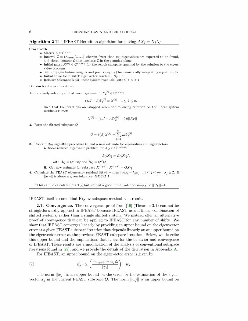
2. Iterative FEAST. “Iterative FEAST” (or IFEAST) is the FEAST algo-rithm implemented such that the linear systems are deliberately solved inaccurately.That is, the linear systems are solved such that the resulting residuals satisfy a conver-gence criteria that is greater (possibly substantially greater) than machine precision.Algorithm 2 summarizes the iterative IFEAST procedure for solving the standardHermitian interior eigenvalue problem.

The implementation of IFEAST requires a new parameter, α, that determines thestopping criterion that is used in solving the linear systems iteratively. Importantly,the stopping criterion changes at each iteration in proportion to the eigenvector resid-uals. IFEAST will not necessarily converge for all values of α (an issue that we dealwith quantitatively in Section 2.1), and so it should be heuristically underestimated.We find that, for example, a value of α = 10−2 tends to work very well in many cases.Any iterative linear system solving algorithm that can be used with general matricescan also be used for solving the linear systems of IFEAST. In this work we consideronly Hermitian matrices A, and we choose to work with MINRES [16] because of itscombination of speed, robustness, and limited storage requirements. Although theFEAST linear systems (zkI − A) are not Hermitian, they can still be solved withMINRES because they are shifted versions of Hermitian systems[6].

In the following subsections we describe the properties of IFEAST analytically.We show that IFEAST can converge linearly when its linear systems are solved in-exactly, and we show how the accuracy of the inexact solves interacts with the otherparameters that govern the behavior of IFEAST. We also examine the relationshipbetween IFEAST and traditional Krylov eigenvalue solving algorithms; because thevast majority of the computation in IFEAST consists of performing calculations withKrylov subspaces in order to solve linear systems, it is natural to ask whether or not


Algorithm 2 The IFEAST Hermitian algorithm for solving AXI = XIΛI

Start with:• Matrix A ∈ Cn×n

• Interval I = (λmin, λmax) wherein fewer than m0 eigenvalues are expected to be found,and closed contour C that encloses I in the complex plane

• Initial guess X(0) ∈ Cn×m0 for the search subspace spanned by the solution to the eigen-value problem

• Set of nc quadrature weights and points (ωk, zk) for numerically integrating equation (4)• Initial value for FEAST eigenvector residual ||RF || a• Relative tolerance α for linear system residuals, with 0 < α < 1

For each subspace iteration i:

1. Iteratively solve nc shifted linear systems for Y(i)k ∈ Cn×m0 .

(zkI −A)Y(i)k = X(i), 1 ≤ k ≤ nc

such that the iterations are stopped when the following criterion on the linear systemresiduals is met:

||X(i) − (zkI −A)Y(i)k || ≤ α||RF ||

2. Form the filtered subspace Q

Q = ρ(A)X(i) =

nc∑k=1

ωkY(i)k

3. Perform Rayleigh-Ritz procedure to find a new estimate for eigenvalues and eigenvectors:i. Solve reduced eigenvalue problem for XQ ∈ Cm0×m0

AQXQ = BQXQΛ

with AQ = QTAQ and BQ = QTQ

ii. Get new estimate for subspace X(i+1): X(i+1) = QXQ

4. Calculate the FEAST eigenvector residual ||RF || = max ||Axj − λjxj ||, 1 ≤ j ≤ m0, λj ∈ I. If||RF || is above a given tolerance, GOTO 1.

aThis can be calculated exactly, but we find a good initial value to simply be ||RF ||=1

IFEAST itself is some kind Krylov subspace method as a result.

2.1. Convergence. The convergence proof from [19] (Theorem 3.1) can not bestraightforwardly applied to IFEAST because IFEAST uses a linear combination ofshifted systems, rather than a single shifted system. We instead offer an alternativeproof of convergence that can be applied to IFEAST for any number of shifts. Weshow that IFEAST converges linearly by providing an upper bound on the eigenvectorerror at a given FEAST subspace iteration that depends linearly on an upper bound onthe eigenvector error at the previous FEAST subspace iteration. Below, we describethis upper bound and the implications that it has for the behavior and convergenceof IFEAST. These results are a modification of the analysis of conventional subspaceiterations found in [22], and we provide the details of the derivation in Appendix A.

For IFEAST, an upper bound on the eigenvector error is given by

(7) ||wj || ≤(|γm0+1|+ αj∆

|γj |

)||wj ||.

The norm ||wj || is an upper bound on the error for the estimation of the eigen-vector xj in the current FEAST subspace Q. The norm ||wj || is an upper bound on


the error for estimating xj in the FEAST subspace at the next iteration, ρ(A)Q.Thevalue γj is the jth largest eigenvalue of ρ(A), with corresponding eigenvector xj . Thedimension of the FEAST search subspace is m0.

If all the shifted linear systems are solved inaccurately with a given convergencecriteria ε on the residual norm, i.e. (ej being the unit vector)

(8) ||Xej −1

ωk(zkI −A)Ykej || ≤ ε, ∀k, j

then the scalar αj can be defined as the ratio of the magnitude of the maximumFEAST linear system residual ε to the value of ||wj ||:

(9) αj = ε/||wj ||.

Also derived in Appendix A, the scalar ∆ is a function of the spectrum of the matrixthat we are diagonalizing, the locations of the FEAST linear system shifts, and thevalues of the FEAST linear system weights:

(10) ∆ =

nc∑k=1

||ωk(zkI −A)−1||.

The criterion for IFEAST to converge for the eigenvector xj comes straightfor-wardly from (7):

(11) αj∆ < |γj | − |γm0+1|.

Provided that the inequality in (11) is true, the FEAST subspace will become a betterapproximation to the eigenvector subspace of interest with each subsequent iteration.IFEAST will converge at the rate of (|γm0+1|+αj∆)/|γj |. The smaller the magnitudeof this coefficient is, the faster FEAST converges by subspace iteration. When thelinear systems of IFEAST are solved exactly (i.e. αj = 0 at machine precision),the convergence rate of traditional FEAST is recovered [25]. In turn, if αj has thesame value at every IFEAST iteration and (11) is satisfied, then the upper bound (7)guarantees linear convergence.

For values of αj∆ that are much smaller than |γm0+1|, IFEAST behaves similarlyto traditional FEAST: solving additional linear systems in parallel leads directly toa better convergence rate. If αj∆ is on the order of, or greater than, |γm0+1|, thenthe behavior of IFEAST is different from that of traditional FEAST. In this case,solving additional linear systems in parallel does not make IFEAST converge faster,and the convergence rate is dominated by the accuracy of the linear system solves. Inaddition, we note that the closer the shifts zk are to the eigenvalues of A, the larger ∆becomes. As a result, the linear systems of IFEAST must be solved to a certain levelof accuracy in order to ensure that all additional shifted linear systems can effectivelycontribute to a faster convergence rate (which can be challenging because using moreshifted systems means that more complex shifts end up closer to an eigenvalue locatedon the real axis). Some eigenvalue problems are also expected to be inherently moredifficult for IFEAST to solve than others, such as, for example, when there is a clusterof eigenvalues located just outside the eigenvalue search interval I = (λmin, λmax),which can have the effect of causing the difference |γj | − |γm0+1| from Equation 11 tobe very small (if m0 is not large enough).

Finally, we point out that the definition for αj in (9) differs from the definition ofα that is used for all eigenvector xj in the IFEAST Algorithm 2. This is by necessity,


as it is not possible to know the maximum norm of the linear system residuals that willensure convergence of the eigenvalue problem (i.e. condition (11)), without havingalready solved the eigenvalue problem. In Algorithm 2, we use the value of the FEASTeigenvector residual ||RF || in place of the eigenvector error ||wj || and heuristicallydetermined the parameter α in order to provide estimates for the linear system residualtolerance.

2.2. Solving Inexact FEAST Linear Systems with GMRES. Unlike thecase for convergence, the results from Proposition 3.8 in [19] can be applied to IFEASTwithout modification. That is, in IFEAST, as with inexact shift-invert iterations, thenumber of GMRES iterations that are required to satisfy the tolerance on the linearsystem residuals (Step 1 in the IFEAST Algorithm 2) generally does not increase asthe eigenvalue problem converges, even though the tolerance itself becomes smaller ateach subsequent IFEAST subspace iteration. We refer the reader to [19] for the detailsof the proof, but point out here that the fundamental reason for this is simple. Thecloser the right hand side of a linear system of equations is to an invariant subspace ofthe coefficient matrix, the fewer GMRES iterations are required to solve the systemto a given tolerance. As IFEAST iterations converge, the right hand sides of theIFEAST linear systems become closer to being invariant subspaces of the matrix thatis being diagonalized (and hence become easier to solve), at the same time as thetolerance for the solution is made more difficult to reach.

This is also the reason that most linear system preconditioners will actually makethe eigenvalue problem more expensive to solve. The right hand sides of the IFEASTlinear systems converge to invariant subspaces of the matrix that is being diagonalized,but they generally do not converge to invariant subspaces of the preconditioned matrix.In order to use a preconditioner with IFEAST without increasing the amount of workthat needs to be done to solve the eigenvalue problem, it is necessary to choose apreconditioner that either shares the eigenvectors of the matrix being diagonalized,or to choose a new preconditioner at each subspace iteration such that the right handsides of the linear systems are invariant subspaces of the preconditioned matrix. Onesuch strategy is described in [4].

This effect also makes it difficult to efficiently apply Algorithm 2 to generalizedeigenvalue problems (1), where the FEAST linear systems become (at iteration i):

(12) (zkB −A)Y(i)k = BX(i).

In this case, unlike the standard eigenvalue problem case, the right hand sides donot converge to an invariant subspace of (zkB − A), and so the number of GMRESiterations that is required for convergence increases with each subspace iteration. Itis always possible to rewrite equation (12) so that the right hand sides do convergeto invariant subspaces of the coefficient matrix, if we consider solving, for example,

(zk − B−1A)Y(i)k = X(i). However, in doing so, we replace our original problem

with another problem of at least equal difficulty; when we replace (zkB − A) with(zk − B−1A), every matrix multiplication by A must be accompanied by a linearsystem solve with B, which dramatically increases the cost of iteratively solving the

corresponding linear system (zk −B−1A)Y(i)k = X(i).

Several authors have suggested some ways of addressing this challenge. Onepossibility involves using tuned preconditioners to recover the desired behavior ofGMRES [5, 26]. Another consists of changing the way the initial guess is chosen forGMRES [9, 27].


3. Relationship between IFEAST and Krylov methods. Standard Kryloveigenvalue solving methods (such as Lanzcos and Arnoldi) work by building a basis Vfor the Krylov subspace K(A,X(0)), using some initial guess X(0) for the eigenvectorsi.e.

(13) V ∈ K(A,X(0)) = span{X(0), AX(0), A2X(0), ..., Ak−1X(0)},

with

(14) X(0) ∈ Cn×m0 , V ∈ Cn×m0k.

For easy comparison with IFEAST below, we consider the case of a block Krylovmethod where the block size is m0 (i.e. size of the FEAST search subspace). Tra-ditional Krylov methods then use the Rayleigh-Ritz procedure to form and solve areduced-dimension eigenvalue problem in order to find approximate eigenpairs in thesubspace K(A,X(0))

(15) (V HAV )XV = (V HV )XV Λ.

Let us assume that the degree (k− 1) of the Krylov subspace (13) is made as large asis practically possible. If the residuals of the approximate eigenpairs from the reducedproblem (15) do not converge, then the method can be “restarted” by using a blockof Ritz vectors X(1) from the solution of (15) as the starting vectors for building anew Krylov subspace K(A,X(1)) of degree (k − 1).

FEAST, when doing the contour integration exactly, forms a subspace by applyinga spectral projector to X(0), which is then also used to solve a reduced-dimensioneigenvalue problem i.e.

(16) Q = ρ(A)X(0) =1

2πi

∮C(zI −A)−1X(0)dz,

(17) (QHAQ)XQ = (QHQ)XQΛ.

We can understand the relationship between FEAST and traditional Krylov meth-ods by considering what happens when the integrand (zI −A)−1X(0) in (16) is eval-uated approximately by using a Krylov subspace. We can rewrite the integral (16)as:

(18) Q = ρ(A)X(0) =1

2πi

∮CY (z)dz,

where Y (z) is the solution to the linear system

(19) (zI −A)Y (z) = X(0).

If we use a Krylov subspace method to find an approximate solution to (19), then


(20) Y (z) = V YV (z), YV (z) ∈ Cm0k×m0 ,

where V is the same Krylov subspace basis from equation (13), and YV is an approx-imate solution to (zI − A)V YV (z) = X(0). Importantly, the Krylov basis V is nota function of z, because the Krylov subspace that is generated by (zI − A) dependsonly on the matrix A and not on the shift z. Because V is independent of z, we canrewrite the expression (18) for Q in such a way that the FEAST reduced-dimensioneigenvalue problem (17) takes a familiar form. Rewriting the expression for Q, we get

(21) Q =1

2πi

∮CY (z)dz = V Gv,

with

(22) Gv ∈ Cm0k×m0 =1

2πi

∮CYV (z)dz.

Then, the FEAST reduced eigenvalue problem (17) becomes

(23) (GHv V

HAV Gv)XQ = (GHv V

HV Gv)XQΛ.

Comparing (23) with (15) makes it clear that IFEAST itself is, in fact, a Krylovsubspace method. The difference between IFEAST and more traditional Krylov meth-ods is that IFEAST uses contour integration to select an ideally-suited linear combi-nation of vectors from the Krylov basis V for finding the desired eigenvalues, withoutfirst having to solve a reduced eigenvalue problem in that basis.

Being able to select the desired eigenvalues in this way can have substantial bene-fits. One of the challenges in using Krylov subspaces is that finding certain eigenvalues,particularly interior eigenvalues or eigenvalues that are clustered closely together, canrequire a subspace basis V of very large dimension. Using a large-dimension subspacebasis V entails large storage requirements for that basis, and a large computationalcost for solving the corresponding reduced eigenvalue problem (15). When usingIFEAST, on the other hand, the dimension of the reduced eigenvalue problem (23) isalways m0, which is substantially smaller than the dimension km0 of the traditionalreduced eigenvalue problem (15).

Moreover, when IFEAST is implemented with a linear system solver that uses ashort recurrence relation (e.g. MINRES), then it can solve eigenvalue problems byusing a Krylov subspace of arbitrarily large dimension without having to form andstore a basis for that subspace; by using short recurrences, IFEAST can form then × m0 matrix product Q = V Gv without forming or storing either the n × km0

matrix V or the km0 ×m matrix Gv. Thus, eigenpairs that would previously havebeen difficult or impossible to obtain due to constraints on the dimension of V becomemuch more tractable to calculate, and the spectrum slicing capability of FEAST ismaintained by making it possible to selectively find specific eigenpairs anywhere inthe spectrum.

The relationship between IFEAST and traditional Krylov methods also offers adifferent perspective on achieving convergence when using restarts. In the context ofIFEAST, a Krylov restart amounts to an approximate subspace iteration with ρ(A)

IFEAST: AN OUTER-INNER ITERATIVE STRATEGY FOR THE FEAST EIGENSOLVER11

for a particular choice of contour C. Using contour integration to choose the subspacewith which to restart ensures that restarting will reliably result in convergence, withinequality (7) giving quantitative answers regarding whether or not restarting willresult in convergence and, if it does, how quickly convergence will occur. IFEASTreverses the process that is used in other restarting strategies [23, 20], in which thesubspace that is used for restarting is determined after solving a reduced eigenvalueproblem in the full Krylov subspace, rather than before.

We elaborate further on the relationship between IFEAST and traditional Krylovtechniques in the following subsections, where we show how the implementation ofIFEAST with particular linear system solvers is related to other Krylov subspacemethods for solving eigenvalue problems. We show that implementing IFEAST us-ing the Full Orthogonalization Method (FOM) is equivalent to traditional explicitlyrestarted block Arnoldi, and that implementing IFEAST using GMRES is closelyrelated to using Harmonic Rayleigh-Ritz for interior eigenvalue problems.

3.1. IFEAST + FOM is Restarted Arnoldi. The block Arnoldi methodconstructs an orthonormal basis V ∈ Cn×m0k of block size m0 and Krylov polynomialdegree k − 1 (for a total dimension of m0k), and then solves a reduced eigenvalueproblem from the Rayleigh-Ritz method in order to find estimates for the desiredeigenvalues and eigenvectors, i.e.

(24) HXV = XV Λ

(25) H = V HAV, V = Kk(A,X(0)), V HV = I

where H ∈ Cm0k×m0k is upper Hessenberg and X(0) ∈ Cn×m0 is the initial guessfor the eigenvectors. If the residuals on the estimated eigenpairs (V XV ,Λ) are notgood enough, then the method can be explicitly “restarted” by building a new Krylovsubspace Kk(A,X(1)) using a new starting block X(1). The new starting block consistsof linear combinations of the estimated eigenvectors, i.e.

(26) X(1) = V XVM

where M ∈ Cm0k×m0 gives the linear combinations that are used to determine eachvector in the new starting block. A variety of different choices for M are possible[22]. A single iteration of IFEAST, when implemented with FOM, produces a newestimate for the eigenvectors of interest X(1) that is equivalent to expression (26) fora particular, natural choice of M .

Implementing IFEAST requires forming a subspace Q ∈ Cn×m0 by evaluating thecontour integral (18), which in turn requires solving linear systems of the form (19).We restate these tasks (respectively) here, i.e.

(27) Q = ρ(A)X(0) =1

2πi

∮CY (z)dz,

(28) (zI −A)Y (z) = X(0).


FOM is used to solve the linear system (28) by forming V using Arnoldi iterations,and then solving a projected linear system [21], i.e.

(29) Y (z) = V(V H(zI −A)V

)−1V HX(0).

Because the linear system matrix (zI − A) is just a shifted version of the originalmatrix A, the solution for Y (z) can be written in terms of the upper Hessenbergmatrix that is generated by the Arnoldi method, i.e.

(30) Y (z) = V (zI −H)−1V HX(0).

Inserting this into the expression for the IFEAST subspace Q (27) , it becomes clearthat using FOM is equivalent to applying the FEAST filter function ρ(λ) to the upperHessenberg matrix H from Arnoldi

(31) Q = V1

2πi

∮C(zI −H)−1dzV HX(0) = V ρ(H)V HX(0).

This is equivalent to filtering out the components of the unwanted Arnoldi Ritzvectors from X(0), leaving only the Ritz vectors whose Ritz values are inside the con-tour C in the complex plane. We can see this by writing the eigenvalue decompositionof H and reordering its eigenvalues and eigenvectors so that the wanted eigenpairs(i.e. the ones whose eigenvalues are inside C) are grouped together, i.e.

(32) H = XV ΛXHV ,

(33) XV = [Xw Xu] , Λ =

[Λw 00 Λu

],

and by writing the initial guess X(0) in terms of its Ritz vector components in the Vsubspace

(34) X(0) = V XwW + V XuU,

where (Xw,Λw) are the m0 wanted Ritz eigenpairs (i.e. the ones whose eigenvalues areinside C in the complex plane), (Xu,Λu) are the (k− 1)m0 unwanted Ritz eigenpairs,and W and U are the components of X(0) in terms of the wanted and unwanted Ritzeigenvectors (respectively). Rewriting (31) in these terms, we get

Q = V [Xw Xu]

[ρ(Λw) 0

0 ρ(Λu)

][Xw Xu]

HV H(V XwW + V XuU)(35)

= V (Xwρ(Λw)W +Xuρ(Λu)U).(36)

IFEAST with FOM thus forms a subspace by filtering the Ritz values and vectorsfrom the Arnoldi Rayleigh Ritz matrix H; the components of X(0) in the direction


of the wanted Ritz vectors are kept roughly the same, and the components of X(0)

in the direction of the unwanted Ritz vectors are substantially reduced. When thecontour integral in (31) is evaluated exactly, then ρ(Λw) = Im0×m0

and ρ(Λu) =0(k−1)m0×(k−1)m0

, and IFEAST forms and solves a reduced eigenvalue problem usingonly the Arnoldi Ritz vectors corresponding to the wanted Ritz values. The vectorsthat are used as the initial guess for the next IFEAST iteration, then, are just thenormalized Arnoldi Ritz vectors corresponding to the Ritz values that are inside thecontour C in the complex plane, i.e.

(37) X(1) = V Xw = V XV

[Im0×m0

0(k−1)m0×m0

].

IFEAST with FOM is equivalent, then, to performing block Arnoldi with a restartstrategy that consists of selecting the desired Ritz vectors and discarding the rest.

In practice this restart strategy can be unreliable for obtaining eigenvalues in theinterior of the spectrum. One perspective on why this happens is that the Rayleigh-Ritz procedure works well for resolving exterior eigenvalues, but not for resolvinginterior ones; restarting with Ritz vectors is thus unreliable for obtaining interioreigenvalues [15]. A remedy for this is to use the Harmonic Rayleigh Ritz procedure [14,15], wherein one solves a different reduced eigenvalue problem that more accuratelyobtains the eigenvalues that are located near some shift.

The fact that the restart strategy (37) is equivalent to using FOM with IFEASTsuggests another perspective on why it is ineffective. Getting IFEAST to convergerequires solving its associated linear systems such that their residuals are sufficientlysmall, and FOM does not minimize the linear system residual for a given subspace.Reliably achieving convergence for interior eigenpairs requires the use of a linearsystem solver that minimizes the linear system residual, such as GMRES or MINRES.

3.2. IFEAST + GMRES is related to Harmonic Rayleigh Ritz. In fact,using GMRES with IFEAST is closely related to using the Harmonic Rayleigh Ritzprocedure. When using GMRES to solve (28) for Y (z), the solution takes the form[21]

(38) Y (z) = V(V H(zI −A)H(zI −A)V

)−1V H(zI −A)HX(0),

where V , again, is the block Arnoldi basis. The IFEAST subspace Q then becomes

(39) Q = V

(1

2πi

∮C

[V H(zI −A)H(zI −A)V

]−1V H(zI −A)HV dz

)X

(0)V ,

where V X(0)V = X(0) is the initial guess X(0) expressed in the Arnoldi basis V .

The integrand in (39) is equivalent to the matrix that one arrives at when usingHarmonic Rayleigh Ritz with Arnoldi. With Harmonic Rayleigh Ritz, one seeks to findapproximations for the eigenvalues that are near some shift z ∈ C, using the subspacebasis V . This is done by solving the reduced, generalized eigenvalue problem [14, 15]

(40) AV (z)XV (z) = BV (z)XV (z)(zI − Λ(z)),


(41) AV (z) = V H(zI −A)H(zI −A)V, BV (z) = V H(zI −A)HV,

where V XV (z) are now the Harmonic Ritz vectors, and Λ(z) are the Harmonic Ritzvalues. In most applications the shift z is taken to be a fixed parameter, but here weare considering a case where it will vary, making the projected matrices AV (z) andBV (z), and the Harmonic Ritz vectors and values XV (z) and Λ(z), into matrix-valuedfunctions of the shift. Like any generalized eigenvalue problem, (40) can be writtenas a standard, non-symmetric eigenvalue problem with a corresponding eigenvaluedecomposition, i.e.

(42) B−1V (z)AV (z) = XV (z)(zI − Λ(z))X−1V (z).

If we note that

(43)[B−1V (z)AV (z)

]−1=[V H(zI −A)H(zI −A)V

]−1V H(zI −A)HV,

then we can use this combined with Equation (42) in order to write the expressionfor Q (39) in terms of the Harmonic Rayleigh Ritz eigenvalue decomposition:

Q = V

(1

2πi

∮C

[B−1V (z)AV (z)

]−1dz

)X

(0)V ,(44)

= V

(1

2πi

∮C

[zI −XV (z)Λ(z)X−1V (z)

]−1dz

)X

(0)V .(45)

Generating the IFEAST subspace by using GMRES is thus equivalent to usingcontour integration to filter the initial guess by using Arnoldi Harmonic Ritz valuesand vectors. Unlike with FOM, however, the resulting contour integral is not equiva-lent to applying the usual FEAST spectral filter ρ(λ) to a projected matrix. Instead,the integration in (45) is the contour integral of the resolvent of a nonlinear eigenvalueproblem, where the eigenvalues and eigenvectors are functions of the complex variablez that are derived from the Harmonic Rayleigh Ritz procedure.

4. Results and Discussions. In this section we illustrate the behavior ofIFEAST using two example matrices.

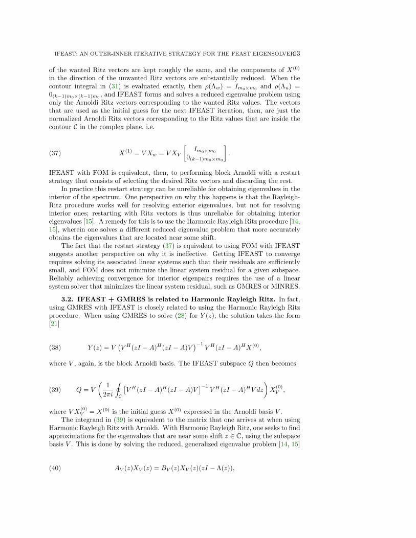
4.1. Example I: Si2. Our first example is the Si2 matrix from the Universityof Florida Sparse Matrix Collection [3]. Si2 is a real symmetric 769 × 769 matrixfrom the electronic structure code PARSEC; it represents the Hamiltonian operatorof a quantum system consisting of two silicon atoms. We illustrate the behavior ofIFEAST by calculating eigenvector/eigenvalue pairs in two places in the spectrum ofSi2: the lowest 20 eigenpairs, and the middle 20 eigenpairs. The eigenvalues, searchcontours, and linear system shifts for each of these calculations are illustrated inFigure 1. Using the same scale, we note that the contour for Interval 1 (the lowesteigenvalues) is much larger than the contour for Interval 2 (the middle eigenvalues)because the eigenvalues in Interval 2 are clustered much more closely together. Dueto the symmetry property of FEAST for addressing the Hermitian problem [18], it isonly necessary to perform the numerical quadrature on the upper-half of the contour


Integration Contour and Linear Shifts for Si2

-1.5

-1.0

-0.5

0.0

0.5

1.0

1.5

-0.5 0.0 0.5 1.0 1.5 2.0 2.5 3.0

Imagin

ary

Part

Real Part

Interval 1 (Lowest 20 Eigenvalues)

15.5 16.2 17.0 17.8 18.5

Real Part

Interval 2 (Middle 20 Eigenvalues)

EigenvaluesLinear System Shifts

Contour

Fig. 1. Locations in the complex plane of the IFEAST integration contour and linear systemshifts. Contour and shifts are provided for two calculations: finding the lowest 20 eigenvalues, andfinding the middle 20 eigenvalues. The quadrature nodes (shifts) are located on a perfect circle(although the contour appears elliptical due to the bounds of the plots). We use here a total of 4linear system shifts for discretizing the integral in the upper-half contours using the Trapezoidal rule.

by using ncup = nc/2 total shifted linear systems. The trapezoidal rule is used toselect the location and weight of each of these shifts.

For a given number of quadrature points nc, subspace size m0 ≥ m (m thenumber of eigenvalues, here 20), equation (7) tells us that a small enough convergencecriterion for the linear systems α guarantees that the FEAST linear convergencecriteria depends entirely on the the value of the filtering function i.e. the outer-iteration subspace iteration. For the Si2 example, in particular, if we select m0 =1.5m = 30 and α ≤ 10−1, IFEAST converges in 9 outer-iterations for both contours(using ncup

= 4). In the following examples we deliberately choose parameter valuessuch that the behavior of IFEAST deviates from that of conventional FEAST, inorder to illustrate the effects of inexact linear sytem solves.

Figure 2 shows the eigenvector residual at each subspace iteration when using theIFEAST Algorithm with MINRES as the linear system solver, the smallest possiblesubspace size of m0 = 20, and the linear system convergence criterion α = 1/2. Inter-val 1 and Interval 2 converge at similar rates by subspace iteration and, as expected,the convergence for each is linear. Unlike with traditional FEAST, however, the num-ber of subspace iterations that is required for convergence is not a good measure of theamount of time needed by IFEAST for solving the eigenvalue problem. Indeed, whensolving the linear systems iteratively, some shifted systems will converge faster thanothers, and some right hand sides will converge faster than others. If enough parallelprocessing power is available to solve all linear system right hand sides simultaneously,then the best measure of the amount of time that a single IFEAST iteration takes isthe number MINRES iterations that is required for the most difficult linear systemright hand side to converge. This is shown in Figure 3. As specified by Proposition3.8 in [19], the number of MINRES iterations required at each FEAST iteration isapproximately constant.

Figure 4 displays this information in a different way, showing the cumulative num-ber of sequential matrix vector products that is required to reach a given eigenvectorresidual when all linear system right hand sides are solved in parallel with MINRES.


Si2: Subspace Iteration Convergence

10-10

10-8

10-6

10-4

10-2

100

0 5 10 15 20 25 30 35 40

Eig

envect

or

Resi

dual

IFEAST Iteration

Lowest 20Middle 20

Fig. 2. Convergence of IFEAST eigenvalue calculations for Si2 by subspace iteration. MINRESis used as the linear system solver, with a subspace dimension of m0 = 20 and a rather large linearsystem convergence criterion of α = 1/2.

Si2: MINRES Iterations at each IFEAST Iteration

0

100

200

300

400

500

600

700

0 5 10 15 20 25 30 35 40

Max M

INR

ES Ite

rati

ons

IFEAST Iteration

Lowest 20Middle 20

Fig. 3. Maximum number of MINRES iterations performed at each IFEAST iteration for Si2,for calculating both the lowest 20 eigenvalues and the middle 20 eigenvalues (see Figure 1). Themaximum number of MINRES iterations is the number of MINRES iterations required by the shiftedlinear system right hand side that takes the longest to converge. When using enough parallelism tosolve all right hand sides simultaneously, this is a measure of the amount of time that each IFEASTiteration takes.

The time required for convergence of the eigenvalue problem is proportional to thenumber of sequential matrix vector products, and so Figure 4 gives the best compar-ison of the performance of IFEAST for Interval 1 and Interval 2.

It is clear from the results in Figure 4 that the convergence for Interval 1 happensmuch quicker than for Interval 2. The reason for this is that the eigenvalues both insideand around Interval 2 are closely clustered together in the middle of the spectrum,whereas the eigenvalues in Interval 1 are well-separated at the lower edge of thespectrum. Any Krylov subspace algorithm will require many more iterations to findthe eigenvalues in Interval 2 than it will for Interval 1, and IFEAST is no exception.


Si2: Matrix Vector Product Convergence

10-10

10-8

10-6

10-4

10-2

100

0 1000 2000 3000 4000 5000 6000 7000 8000

Eig

envect

or

Resi

dual

Sequential Matrix Vector Products

Lowest 20Middle 20

Fig. 4. Convergence of IFEAST eigenvalue calculations for Si2 by number of sequential matrixvector multiplications, for both the lowest 20 eigenvalues and the middle 20 eigenvalues (see Figure1). The number of sequential matrix vector multiplications is the sum of the number of MINRESiterations for the slowest-converging linear system right hand side at each IFEAST iteration. Thisis the best measure of the amount of time that IFEAST requires to converge when solving all linearsystem right hand sides in parallel at each subspace iteration.

However, one benefit of implementing IFEAST with MINRES is that, unlike withother Krylov eigenvalue methods, the size of the subspace needed for calculatingthe eigenpairs in Interval 2 is exactly the same as the size of the subspace neededfor calculating the eigenpairs in Interval 1. This makes it possible to maintain theparallelism of traditional FEAST by solving for many eigenpairs in parallel by usingmultiple contours.

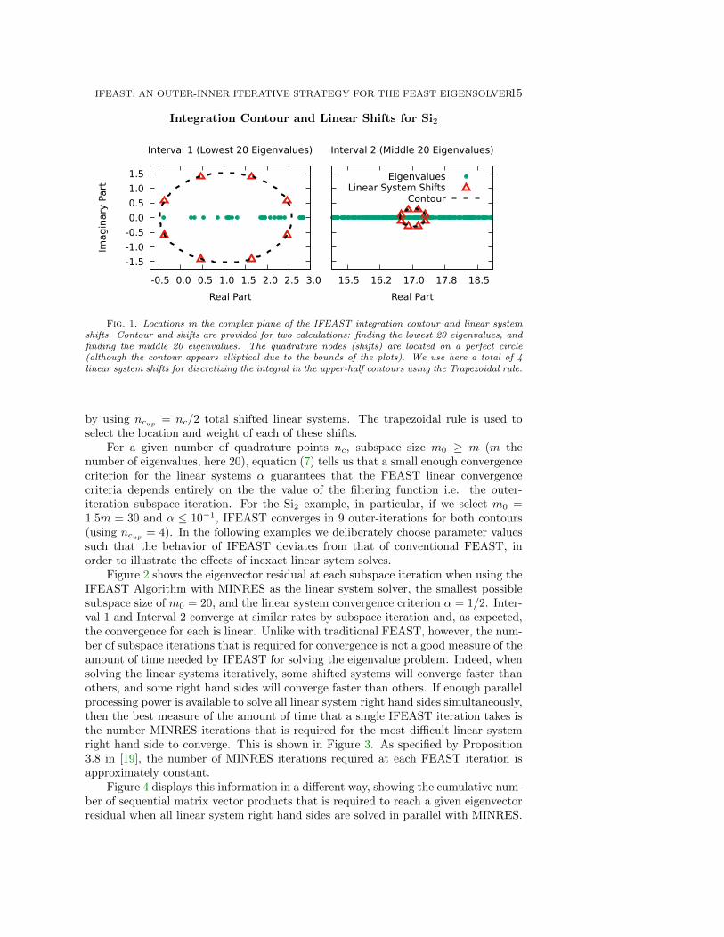
In traditional FEAST, the rate of convergence by subspace iteration can alwaysbe improved by increasing the accuracy of the numerical integration of Equation (4),usually by increasing the number of terms in the quadrature rule (5). As discussed inSection 2.1, the situation is less simple in IFEAST, due to the relationship betweenconvergence and the accuracy of the linear system solutions. In general, increasingthe number of shifted linear systems in the quadrature rule (5) will improve the con-vergence rate by subspace iteration up to the point that convergence becomes limitedby the accuracy of the linear system solutions, after which increasing the number ofquadrature points will no longer improve convergence. This effect is illustrated inFigure 5, which shows the convergence of IFEAST by subspace iteration for severalnumbers of linear system shifts. Here we calculate the 20 eigenpairs inside Interval2 (see Figure 1) by using a subspace size of m0 = 25, with MINRES again as thelinear system solver and a convergence criterion α = 1/2. With these parameters, in-creasing the number of shifted linear systems ncup

from 4 to 10 increases the subspaceiteration convergence rate considerably, but increasing the number of shifted linearsystems from 10 to 24 barely changes the convergence rate at all.

As previously mentioned, the convergence rate by subspace iteration is not atrue measure of the performance of IFEAST; a better measure of performance isthe number of matrix vector products that is required to reach a given eigenvectorresidual when all linear system right hand sides are solved in parallel. Figure 6shows the convergence of IFEAST versus the number of sequential matrix vectorproducts for the same numerical experiment, where we calculate the 20 eigenpairs


Si2: Subspace Iteration Convergence forDifferent Numbers of Shifted Systems

10-1210-1010-810-610-410-2100

0 2 4 6 8 10 12

Eig

envect

or

Resi

dual

IFEAST Iteration

4 Shifts10 Shifts24 Shifts

Fig. 5. Eigenvector residual versus IFEAST iteration for calculating the 20 eigenvalues inInterval 2 (the middle eigenvalues of Si2; see Figure 1), using several different numbers of shiftedlinear systems ncup in the upper-half contour, and for a constant subspace size of m0 = 25. In-creasing the number of shifted systems that are solved in parallel improves the convergence rate upto the point that convergence becomes limited by the accuracy of the linear system solves.

Si2: Matrix Vector Product Convergence forDifferent Numbers of Shifted Systems

10-1210-1010-810-610-410-2100

0 1000 2000 3000 4000 5000 6000 7000 8000

Eig

envect

or

Resi

dual

Sequential Matrix Vector Products

4 Shifts10 Shifts24 Shifts

Fig. 6. Eigenvector residual versus number of required sequential matrix vector multiplicationsfor calculating the 20 eigenvalues in Interval 2 (the middle eigenvalues of Si2; see Figure 1), usingseveral different numbers of shifted linear systems. All shifted linear system right hand sides areassumed to be solved in parallel. Increasing the number of shifted linear systems can cause IFEASTto take longer to converge when doing so brings some of those shifts closer to the eigenvalues of thematrix without also increasing the subspace iteration convergence rate.

inside Interval 2 by using several different numbers of shifted linear systems. Whenlooking at the required number of matrix vector products, increasing the number ofshifted linear systems from 4 to 10 improves performance, but increasing the numberof shifted linear systems from 10 to 24 actually decreases performance, resulting inIFEAST taking longer to converge. Although the shifted linear systems are solved in


Na5: Matrix Vector Product Comparison for IFEAST and Arnoldi

Subspace Size 75 100 200 787

IFEAST Iterations 11 11 11 10Arnoldi Restarts 57 23 5 0

IFEAST Total Matvec 34,819 44,212 105,283 463,691IFEAST Sequential Matvec 672 498 368 278Arnoldi Matvec 946 854 844 787

Table 1Comparison of the number of matrix vector products required to calculate the 50 lowest eigen-

pairs of Na5 to an eigenvector residual of 10−10, using both IFEAST and Arnoldi (from the packageARPACK). Matrix vector product counts are shown for several subspace sizes. The IFEAST “To-tal Matvec” is the total number of matrix vector products that IFEAST requires, and the IFEAST“Sequential Matvec” is the number of matrix vector products that must be done sequentially if all ofthe matrix vector products that can be done in parallel are performed in parallel.

parallel, some of the linear systems are more difficult to solve than others, becausetheir shifts are closer to the real axis (and are thus closer to the eigenvalues). Dueto the limited accuracy of the linear system solves, the convergence rate by subspaceiteration remains essentially the same for both 10 and 24 shifts. As a result, IFEASTrequires more time when using 24 shifts because it needs to do more work to solvethe linear systems that are closer to the real axis, while at the same time the limitedaccuracy of the linear system solves prevents it from converging more quickly.

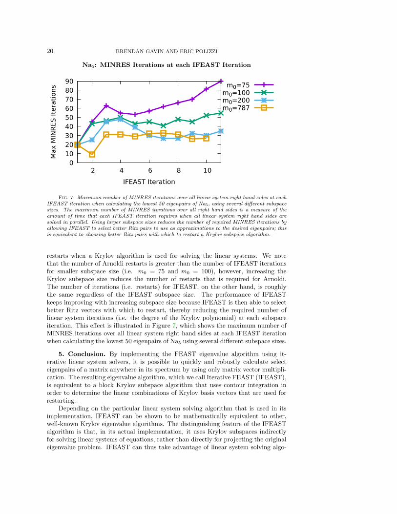
4.2. Example II: Na5. Our second example is the Na5 matrix, also from theUniversity of Florida Sparse Matrix Collection [3]. Na5 is a real symmetric 5832×5832matrix from the electronic structure code PARSEC, and it represents the Hamiltonianoperator of a quantum system consisting of five sodium atoms. In order to providecontext for the performance of IFEAST, we calculate the 50 lowest eigenvalue/eigen-vector pairs for Na5 using both IFEAST and Arnoldi. The implementation of Arnoldithat we use is ARPACK [1], which implements single vector Arnoldi with implicitrestarts.

Table 1 shows the number of matrix vector products that is required to calculatethe 50 lowest eigenvalue/eigenvector pairs of Na5 to an eigenvector residual of 10−10

using both IFEAST and Arnoldi. The results are shown for several different valuesof subspace size. For IFEAST, the subspace size is the value of the parameter m0

in the IFEAST algorithm, which is the size of the subspace that is used for theFEAST subspace iterations. For Arnoldi, the subspace size is the maximum size ofthe Krylov subspace for ARPACK. IFEAST is run by using 4 linear system shifts inthe upper-half contour, that are chosen by using the trapezoidal rule, and a linearsystem convergence criterion of α = 1/5. MINRES is used as the linear system solver.

IFEAST generally requires a substantially larger total number of matrix vectorproducts than Arnoldi does. However, if the available parallelism in the IFEASTalgorithm is fully utilized, meaning that all matrix vector products are performed inparallel, then the relative number of matrix vector products that must be done se-quentially becomes competitive in comparison with Arnoldi. In other words, althoughIFEAST has to do much more work than Arnoldi, it can be made to converge fasterin time by doing most of that work in parallel.

Table 1 also compares the number of IFEAST iterations to the number of Arnoldirestarts; as described in Section 3, IFEAST subspace iterations are equivalent to


Na5: MINRES Iterations at each IFEAST Iteration

0 10 20 30 40 50 60 70 80 90

2 4 6 8 10

Max M

INR

ES Ite

rati

ons

IFEAST Iteration

m0=75m0=100m0=200m0=787

Fig. 7. Maximum number of MINRES iterations over all linear system right hand sides at eachIFEAST iteration when calculating the lowest 50 eigenpairs of Na5, using several different subspacesizes. The maximum number of MINRES iterations over all right hand sides is a measure of theamount of time that each IFEAST iteration requires when all linear system right hand sides aresolved in parallel. Using larger subspace sizes reduces the number of required MINRES iterations byallowing IFEAST to select better Ritz pairs to use as approximations to the desired eigenpairs; thisis equivalent to choosing better Ritz pairs with which to restart a Krylov subspace algorithm.

restarts when a Krylov algorithm is used for solving the linear systems. We notethat the number of Arnoldi restarts is greater than the number of IFEAST iterationsfor smaller subspace size (i.e. m0 = 75 and m0 = 100), however, increasing theKrylov subspace size reduces the number of restarts that is required for Arnoldi.The number of iterations (i.e. restarts) for IFEAST, on the other hand, is roughlythe same regardless of the IFEAST subspace size. The performance of IFEASTkeeps improving with increasing subspace size because IFEAST is then able to selectbetter Ritz vectors with which to restart, thereby reducing the required number oflinear system iterations (i.e. the degree of the Krylov polynomial) at each subspaceiteration. This effect is illustrated in Figure 7, which shows the maximum number ofMINRES iterations over all linear system right hand sides at each IFEAST iterationwhen calculating the lowest 50 eigenpairs of Na5 using several different subspace sizes.

5. Conclusion. By implementing the FEAST eigenvalue algorithm using it-erative linear system solvers, it is possible to quickly and robustly calculate selecteigenpairs of a matrix anywhere in its spectrum by using only matrix vector multipli-cation. The resulting eigenvalue algorithm, which we call Iterative FEAST (IFEAST),is equivalent to a block Krylov subspace algorithm that uses contour integration inorder to determine the linear combinations of Krylov basis vectors that are used forrestarting.

Depending on the particular linear system solving algorithm that is used in itsimplementation, IFEAST can be shown to be mathematically equivalent to other,well-known Krylov eigenvalue algorithms. The distinguishing feature of the IFEASTalgorithm is that, in its actual implementation, it uses Krylov subspaces indirectlyfor solving linear systems of equations, rather than directly for projecting the originaleigenvalue problem. IFEAST can thus take advantage of linear system solving algo-


rithms like MINRES or BICGSTAB that do not need to store a basis for the Krylovsubspace. This makes it possible to solve an eigenvalue problem by implicitly using avery large Krylov subspace without ever having to store a basis for it.

In being able to solve for select eigenvalue/eigenvector pairs using an almostarbitrarily small amount of storage, IFEAST retains the spectrum slicing propertyof traditional FEAST, making it possible to solve for large numbers of eigenpairs inparallel. The IFEAST algorithm also retains many of the other parallel characteristicsof traditional FEAST (such as solving multiple linear systems, and multiple righthand sides, in parallel), with the caveat that the benefits of this parallelism can bediminished when the shifted linear systems are solved too inaccurately relative to theaccuracy of quadrature rule for the FEAST contour integration.

As described in Section 2.2, future research directions will include applying thework of previous authors [9, 5, 26, 27] to IFEAST in order to try to make it as efficientfor the generalized eigenvalue problem as it is for the standard eigenvalue problem.

Appendix A. FEAST Convergence Bounds.In this section we show how to derive the upper bound on the eigenvector error

for inexact FEAST

(46) ||xj − qj || ≤(|γm0+1|+ αj∆

|γj |

)||xj − qj ||.

The upper bound in (46) can be derived using a modification of the method forfinding an upper bound on the eigenvector error that is used in analyzing standardsubspace iterations [22].

A.1. Standard Subspace Iterations. With standard subspace iterations, wewant to find the eigenvectors corresponding to the m0 largest-magnitude eigenvaluesof a matrix A ∈ Cn×n. This is done by repeatedly multiplying an approximatesubspace Q ∈ Cn×m0 by A, and reorthogonalizing the column vectors of Q in betweenmultiplications (using Rayleigh-Ritz, for example). The usual method for provingconvergence is to show that, for every eigenvector xj , 1 ≤ j ≤ m0, an upper bound onthe error of its estimation in the subspace Q goes down after each subspace iteration.This can be done by judiciously choosing a vector qj ∈ Q that is close to xj andshowing that there is always a different vector qj ∈ AQ that is closer to xj than qj is.

Let X1 ∈ Cn×m0 be the subspace whose column vectors are the eigenvectors thatwe want to find, and X2 ∈ Cn×(n−m0) be the subspace composed of the other n−m0

eigenvectors. Then the vector qj is usually chosen to be the unique vector in Q thatsatisfies

(47) X1XT1 qj = xj .

In that case, the difference vector wj = qj−xj is spanned exactly by X2, since X1 andX2 are mutually orthogonal, invariant subspaces of A. The vector qj is then chosento be

(48) qj =1

λjAqj ,


where λj is the eigenvalue corresponding to the eigenvector xj . The difference vectorwj = qj−xj is then also spanned exactly by X2, a fact that we can use to relate ||wj ||to ||wj || i.e.

qj =1

λjAqj =

1

λj(Axj +Awj) = xj +

1

λjAwj ,(49)

wj = qj − xj =1

λjAwj ,(50)

||wj || =1

|λj |||Awj || ≤

|λm0+1||λj |

||wj ||,(51)

where we know that ||Awj || ≤ |λm0+1|||wj || because wj is spanned exactly by X2,the (n−m0) eigenvectors corresponding to the eigenvalues with magnitudes less thanor equal to |λm0+1|. Equation (51) shows that an upper bound on the error for theestimation of xj in the subspace Q always decreases when Q is multiplied by A, andthat it does so at a rate that is linear and proportional to the ratio between λm0+1 andλj . Thus, subspace iterations are guaranteed to converge faster when the subspace Qis larger and when the eigenvalues of A are more separated.

A.2. Inexact FEAST. We can find a similarly informative upper bound withwhich to analyze the convergence of iterative FEAST by following a similar line ofreasoning. Traditional FEAST can be interpreted as a subspace iteration that usesthe matrix ρ(A) instead of the original matrix A,

(52) A −→ ρ(A) =

nc∑k=1

ωk(zkI −A)−1.

Then the upper bound (51) becomes

(53) ||wj || ≤|γm0+1||γj |

||wj ||,

where γj is the jth largest eigenvalue of ρ(A), with corresponding eigenvector xj .The γj with the largest magnitudes correspond to the ‘wanted’ eigenvalues of A thatlie inside of the integration contour (4). Making the quadrature rule (5) more ac-curate by increasing the number of quadrature points nc has the effect of makingthe ratio |γm0+1|/|γj | smaller, which is how standard FEAST can improve its rate ofconvergence by solving more linear systems.

Equation (53) requires modification when the linear systems of FEAST are solvedinexactly. In particular, if we apply ρ(A) by solving the linear systems

(54)1

ωk(zkI −A)yk,j = qj , ∀k = 1, . . . , nc, ∀j = 1, . . . ,m0

such that there is some error sk,j in the solution of the linear system, i.e.

(55) sk,j = ωk(zkI −A)−1qj − yk,j ,


then, for inexact FEAST, equation (48) becomes

(56) qj =1

γj

(ρ(A)qj −

nc∑k=1

sk,j

).

This is not necessarily very useful in practice, however, because the values of sk,j arenot known. Instead, (56) can be rewritten in terms of the linear system residuals, thenorms of which are used as the stopping criteria for iterative linear system solvers:

(57) qj =1

γj

(ρ(A)qj −

nc∑k=1

ωk(zkI −A)−1rk,j

),

with

(58) rk,j = qj −1

ωk(zkI −A)yk,j .

Since qj = wj + xj , we can derive the expression for wj from (57):

(59) wj = qj − xj =1

γj

(ρ(A)wj −

nc∑k=1

ωk(zkI −A)−1rk,j

).

We can then find an upper bound similar to (53):

(60) ||wj || ≤|γm0+1||γj |

||wj ||+1

|γj |

nc∑k=1

||ωk(zkI −A)−1|| ||rk,j ||.

Assuming that all the linear systems (54) are solved using iterative solvers with thesame convergence criteria ε on the residual norm, then ||rk,j || ≤ ε, ∀k, j, we get:

(61) ||wj || ≤(|γm0+1|+ αj∆

|γj |

)||wj ||,

with

(62) αj = ε/||wj ||,

and

(63) ∆ =

nc∑k=1

||ωk(zkI −A)−1||.

If the linear systems are solved such that αj is the same at every FEAST subspace it-eration, then linear convergence is guaranteed, with the rate of convergence dependingon accuracy of the linear system solutions.

Acknowledgment: We thank Alessandro Cerioni and Antoine Levitt for bringingtheir FEAST-GMRES experiment results to our attention. We thank Yousef Saadand Peter Tang for useful discussions. This material is supported by Intel and NSFunder Grant #CCF-1510010.

REFERENCES


[1] ARPACK. http://www.caam.rice.edu/software/ARPACK/. Accessed: 2016-03-15.[2] J. Berns-Muller, I. G. Graham, and A. Spence, Inexact inverse iteration for symmetric

matrices, Linear Algebra and its Applications, 416 (2006), pp. 389–413.[3] T. Davis and Y. Hu, The university of florida sparse matrix collection, ACM Transactions on

Mathematical Software, 38 (2011), http://www.cise.ufl.edu/research/sparse/matrices.[4] M. A. Freitag and A. Spence, A tuned preconditioner for inexact inverse iteration applied to

hermitian eigenvalue problems, IMA journal of numerical analysis, 28 (2008), pp. 522–551.[5] M. A. Freitag, A. Spence, and E. Vainikko, Rayleigh quotient iteration and simplified jacobi-

davidson with preconditioned iterative solves for generalised eigenvalue problems, Techn.report, Dept. of Math. Sciences, University of Bath, (2008).

[6] R. Freund, On conjugate gradient type methods and polynomial preconditioners for a class ofcomplex non-hermitian matrices, Numerische Mathematik, 57 (1990), pp. 285–312.

[7] P. Giannozzi, S. Baroni, N. Bonini, M. Calandra, R. Car, C. Cavazzoni, D. Ceresoli,G. L. Chiarotti, M. Cococcioni, I. Dabo, et al., Quantum espresso: a modular andopen-source software project for quantum simulations of materials, Journal of physics:Condensed matter, 21 (2009), p. 395502.

[8] G. H. Golub and C. F. Van Loan, Matrix computations, vol. 3, JHU Press, 2012.[9] G. H. Golub and Q. Ye, Inexact inverse iteration for generalized eigenvalue problems, BIT

Numerical Mathematics, 40 (2000), pp. 671–684.[10] S. Guttel, E. Polizzi, P. T. P. Tang, and G. Viaud, Zolotarev quadrature rules and load

balancing for the feast eigensolver, SIAM Journal on Scientific Computing, 37 (2015),pp. A2100–A2122, https://doi.org/10.1137/140980090.

[11] V. Kalantzis, J. Kestyn, E. Polizzi, and Y. Saad, Domain decomposition approaches foraccelerating contour integration eigenvalue solvers for symmetric eigenvalue problems,preprint, (2016).

[12] J. Kestyn, E. Polizzi, and P. T. Peter Tang, Feast eigensolver for non-hermitian problems,SIAM Journal on Scientific Computing, 38 (2016), pp. S772–S799.

[13] Y.-L. Lai, K.-Y. Lin, and W.-W. Lin, An inexact inverse iteration for large sparse eigenvalueproblems, Numerical Linear Algebra with Applications, 4 (1997), pp. 425–437.

[14] R. B. Morgan, Computing interior eigenvalues of large matrices, Linear Algebra and itsApplications, 154 (1991), pp. 289–309.

[15] R. B. Morgan and M. Zeng, Harmonic projection methods for large non-symmetric eigen-value problems, Numerical linear algebra with applications, 5 (1998), pp. 33–55.

[16] C. C. Paige and M. A. Saunders, Solution of sparse indefinite systems of linear equations,SIAM journal on numerical analysis, 12 (1975), pp. 617–629.

[17] PARDISO. http://www.pardiso-project.org/. Accessed: 2016-03-15.[18] E. Polizzi, Density-matrix-based algorithm for solving eigenvalue problems, Phys. Rev. B, 79

(2009), p. 115112.[19] M. Robbe, M. Sadkane, and A. Spence, Inexact inverse subspace iteration with precondi-

tioning applied to non-hermitian eigenvalue problems, SIAM Journal on Matrix Analysisand Applications, 31 (2009), pp. 92–113.

[20] Y. Saad, Chebyshev acceleration techniques for solving nonsymmetric eigenvalue problems,Mathematics of Computation, 42 (1984), pp. 567–588.

[21] Y. Saad, Iterative methods for sparse linear systems, SIAM, 2003.[22] Y. Saad, Numerical Methods for Large Eigenvalue Problems: Revised Edition, SIAM, 2011.[23] D. C. Sorensen, Implicit application of polynomial filters in a k-step arnoldi method, Siam

journal on matrix analysis and applications, 13 (1992), pp. 357–385.[24] P. T. P. Tang, J. Kestyn, and E. Polizzi, A new highly parallel non-hermitian eigensolver,

in Proceedings of the High Performance Computing Symposium, Society for ComputerSimulation International, 2014, p. 1.

[25] P. T. P. Tang and E. Polizzi, Feast as subspace iteration accelerated by approximate spectralprojection, SIAM Journal on Matrix Analysis and Applications, 35 (2014), p. 354390.

[26] F. Xue and H. C. Elman, Fast inexact subspace iteration for generalized eigenvalue problemswith spectral transformation, Linear Algebra and its Applications, 435 (2011), pp. 601–622.

[27] Q. Ye and P. Zhang, Inexact inverse subspace iteration for generalized eigenvalue problems,Linear Algebra and its Applications, 434 (2011), pp. 1697–1715.

http://www.caam.rice.edu/software/ARPACK/

http://www.cise.ufl.edu/research/sparse/matrices

https://doi.org/10.1137/140980090

http://www.pardiso-project.org/

AN IMPROVED KRYLOV EIGENVALUE STRATEGY USING THE … · AN IMPROVED KRYLOV EIGENVALUE STRATEGY...

Documents

Transcript of AN IMPROVED KRYLOV EIGENVALUE STRATEGY USING THE … · AN IMPROVED KRYLOV EIGENVALUE STRATEGY...