AN IMPLICIT NUMERICAL SOLUTION

OF THE TURBULENT THREE-DIMENSIONAL INCOMPRESSIBLE

BOUNDARY-LAYER EQUATIONS

by

William Frederick Klinksiek

Thesis Submitted to the Graduate Faculty of the

Virginia Polytechnic Institute and State University

in Partial Fulfillment of the Requirements for the Degree of

DOCTOR OF PHILOSOPHY

in

Mechanical Engineering

APPROVED: F .. J. Pierce

Dr. H. L. Wood

Dr. R. A. Comparin

June, 1971

Blacksburg~ Virginia

LD 5C,55 VS5 0 11 7 I J{4-5 c. 2

ACKNOWLEDGEMENTS

The author gratefully acknowledges Dr. J. B. Jones for

employing him as an Instructor in the Mechanical Engineering

Department which allowed the author to further advance his

graduate training. The author further extends his gratitude

to the Army Research Office-Durham for partially funding this

investigation which is part of a total research grant made to

Dr. F. J. Pierce.

It has been a privilege to have Drs. F. J. Pierce (Chairman),

J. B. Jones, R. A. Comparin, H. L. Wood and C. K. Martin as his

advisory committee and the author extends his sincere appreciation

for their advice, time, criticism and encouragement during the

preparation of this thesis.

In addition, the author expresses his gratitude to

Miss Willie Mae Hylton for typing the major portion of the

manuscript.

Finally, to his wife t Sharon, the author expresses his

appreciation for her understanding, patience, and encouragement

during the past four years.

ii

TABLE OF CONTENTS

TITLE PAGE • • • • i

ACKNOWLEDGEMENTS • ii

TABLE OF CONTENTS • iii

LIST OF FIGURES v

TABLE OF NOMENCLATURE •• viii

I. INTRODUCTION... 1

II. REVIEW OF LITERATURE • 3

III. INVESTIGATION •••• 8

A. The Governing Equations 8

B. The Eddy-Viscosity Model . 13

C. Finite Difference Formulation 15

1. Two-Dimensional and Plane of Symmetry Formulation 16

2. Three-Dimensional Formulation ••.• 23

D. Generation of Boundary Conditions and Initial Conditions 31

E. Solution Technique . . . . . . 39

F. The Continuity Equation 42

G. Stability and Convergence . 44 . . . IV. RESULTS . . . . . . . . 52

A. Laminar Two-Dimensional Solution • 52

B. Turbulent Two-Dimensional Flow •• 60

C. Plane of Symmetry and Three-Dimensional Results 73

V. SUMMARY AND CONCLUSIONS . .• 106

iii

iv

VI. BIBLIOGRAPHY ••••••.•••

VII. APPENDIX A (Computer Program)

VIII. VITA • . . . • • . • • • . •

Page 109

114

. • . · • · • . · 145

3.1

3.2

3.3

3.4

3.5

3.6

4.1

4.2

4.3

4.4

4.5

4.6

4.7

4.8

4.9

LIST OF FIGURES

Two-Dimensional Finite Difference Grid • •

Three-Dimensional Finite Difference Grid .

Schematic Drawing of Johnston's Test Geometry.

Schematic Drawing of Hornung and Joubert's Test Geometry • • • • • • • . • . • •

Experimental Station Locations for Johnston's Test Geometry • • • • • • • • • . • •

Experimental Station Locations for Hornung and Joubert's Test Geometry. • • •. • •.••.

V-Velocity Profile Compared with Blasius Solution for hX = 0 .•• • • • . . . .

V-Velocity Profile Compared with Blasius Solution for hX = o •••••••••••

U-Velocity Profile Compared with Blasius Solution for hX = 0/2 and l1X = 40 ••••

V-Velocity Profile Compared with Blasius Solution for l1X = 0/2 and l1X = 40.

Skin-Friction Coefficient Compared with Blasius Solution

Development of Streamwise Turbulent Velocity Profiles Compared with the Law of the Wall .

* Development of GIl and 01 Compared with a Momentum Integral Analys1s • • . • • • • .

Turbulent Skin-Friction Coefficient Compared with the Ludwieg and Tillmann Correlation . • • •

Initial Law of the Wall Fit to Schubauer and Klebanoff's Experimental Data at X = 19.0 ft •.

v

17

24

32

33

35

37

53

54

55

56

57

61

63

64

66

4.10

4.11

4.12

4.13

4.14

4.15a

4.l5b

4.l5c

4.l5d

4.16

4.17

4.1S

4.l9a

4.l9b

vi

Initial U-Velocity Profile for Schubauer and Klebanoff Geometry in Physical Coordinates at X = 19.0 ft • • • • • • • • • • • • • • 67

U-Velocity Profile Compared with Schubauer and Klebanoff's Experimental Data at X = 20.5 ft. 69

U-Velocity Profile Compared with Schubauer and Klebanoff's Experimental Data at X = 21.5 ft. 70

Initial U-Velocity Profile fit to Johnston's Experimental Data at Station D-S • • • • . • 74

External Velocity Field on the Plane of Symmetry for the Johnston Geometry • • . • 75

IT-Velocity Profile Compared with Johnston's Experimental Data at Station D-6 • • • • • • 78

U-Velocity Profile Compared with Johnston's Experimental Data at Station D-XS • • . . . 79

U-Ve1ocity Profile Compared with Johnston's Experimental Data at Station D-4 • • • • • • 80

U-Ve1ocity Profile Compared with Johnston's Experimental Data at Station D-X6 • • • • • 81

Cross-Flow Velocity Gradients Compared with Johnston's Experimental Data at Station D-X6 82

Development of 911 on the Plane of Symmetry . Compared with Jonnston's Experimental Data. 84

'Ie Development of 0 on the Plane of Symmetry Compared with Jo~nston's Experimental Data

U~ and W~Velocity Profiles Compared with Johnstonts Experimental Data at Stations B-4

85

and F-4 • . • . • • • . . . • • • . • . .• 86

Us and WgVelocity Profiles Compared with Johnston's Experimental Data at Stations A-4 and G-4 • • • • • • • . • . . • • . • • 87

4.20a

4.20b

4.21

4.22

4.23

4.24

4.25

4.26

4.27

4.28

4.29

4.30

4.31

vii

Us and W-Velocity Profiles Compared with Johnston~s Experimental Data at Stations B-X6 and F-X6 • • . • • • • • • • • • • •

Us and W-Velocity Profiles Compared with Johnston~s Experimental Data at Stations

88

A-X6 and G-X6 • • • • • • • • • • • • • • • 89

Variation of Angle of Skewing Compared with Johnston's Experimental Data at Stations A-4 and G-4 • . • • • • • • • • • • • . . . 91

Variation of Angle of Skewing Compared with Johnston's Experimental Data at Stations B-X6 and F-X6 • • • • • • • • • • • . • . • • •. 92

Variation of Angle of Skewing in the Near Wall Region Compared with Johnston's Experimental Data at Stations B-X6 and F-X6 • • . . • 93

Development of 911 off the Plane of Symmetry Compared with Jonnston's Experimental Data. 94

* Development of 0 off the Plane of Symmetry Compared with Jonnston's Experimental Data. 95

Development of 913 off the Plane of Symmetry Compared with Jonnston's Experimental Data. 96

U-Velocity Profile Compared with Hornung and Joubert's Experimental Data at Station 10 .• 99

Us and WsVelocity Profiles Compared with Hornung and Joubert's Experimental Data at Station 12 •• 100

Us and WsVelocity Profiles Compared with Hornung and Joubert's Experimental Data at Station 14 .. 101

Variation of the X Component of the Laminar and Turbulent Shear Stress • • • • • • • • . . • 104

Variation of the Z Component of the Laminar and Turbulent Shear Stress . • •. •.•. 105

A

A*

Aeff

A' (j)

C' (j)

Di(j)

D' , (j) i

Dij

D •. 1J

Fi

Fi(j)

G

H

L

p

p

p'

TABLE OF NOMENCLATURE

van Driest's damping factor

Distance of origin translation

Modified value of A

Matrix coefficient

Matrix coefficient

Matrix coefficients

Matrix coefficients

Instantaneous rate-of-strain tensor:

Time average rate-of-strain tensor:

Recurrence coefficients

Function

Body force vector

Recurrence coefficients

Function

Dunnny variable

Nondimensionalized mixing length

Instantaneous pressure

Time average pressure

Turbulent pressure fluctuation

Reference velocity

Velocity vector with components (U, V, W)

Time average velocity vector with components (U, V, W)

viii

Q~ l.

Qs 00

QOOi

S~ (j)

TE

X. l.

b

e, exp

i, j, k

t

r l , r 2 ,

sl' s2' 8 4, s5'

s7' ss'

u, v, w

u, v, w

uoo ' w 00

uoo ' w 00

U s' W s

u*

+ u

r3

S3} s6' t

ix

Turbulent velocity fluctuation vector with components (U', Vi, W')

External streamline coordinate velocity

External velocity vector with components (Uoo ' Voo ' Woo)

Matrix Coefficients

Truncation error

Displacement vector with components (X, Y, Z)

Reference length

Exponentiation with respect to the Naperian base

Indices

Mixing length

Coefficients defined in Eq. 3.23

Coefficients defined in Eqs. 3.23 and 3.31

Nondimensionalized velocity components corresponding to fi, V, and W respectively

Space averaged velocity components in finite difference grid

Nondimensionalized external velocity components corresponding to Uoo and Woo' respectively

Spaced average external velocity components in finite difference grid

Streamline coordinate velocity components

1

Shear velocity = (;w)2 U --k U

wz

wz

wz co

wz co

x, y, z

+ Y

6x, 6Y+,} 6y_, 6z

a. s

a., S, y

E

E m

11'

p

x

dW az (nondimensionalized)

Space average value of wz in finite difference grid

External value of wz

Space average value of wz in finite difference grid co

Nondimensional displacements corresponding to X, Y, and Z, respectively

Yu* v

Finite difference increments

Angle of skewing with respect to free stream stream­line coordinate direction

Amplification factors

Boundary-layer thickness

Displacement thicknesses with respect to streamline coordinates

Eddy viscosity

Nondimensionalized eddy viscosity

Parameter defined in Eq. 3.57

Momentum thicknesses with respect to streamline coordinates

Dynamic viscosity

Kinematic viscosity

3.1415926 •••

Density

Step size parameter

Components of the laminar shear stress in the X and Z directions, respectively

Components of the turbulent shear stress in the X and Z directions, respectively

T T W W

X Z

T W

xi

Wall shear stresses in the X and Z directions, respectively

Total wall shear stress

Parameter defined in Eq. 3.57

I. INTRODUCTION

For many years momentum integral techniques have been used to pre­

dict the growth and general characteristics of two-dimensional turbulent

boundary-layer flows. Not until large digital computers were introduced

were numerical solutions of the two-dimensional boundary-layer equations

feasible. With the development of such computers, and because of the

large quantity of empirical input which momentum integral methods require,

Spalding [1], in his recent review of the state of the art, recommended

abandonment of any further effort in this area, favoring instead numeri­

cal solution techniques applied directly to the governing partial

differential equations.

For three-dimensional turbulent boundary-layer flows, the momentum

integral approach requires even more empirical input. The general case

has two momentum integral equations, one each for the free-stream and

transverse directions, and at least seven unknowns. For example, in

addition to a velocity profile model in the free-stream direction, an ad­

ditional empirical model must be introduced for the cross-flow velocity

profile. A wall shear stress correlation is required, and except for

the recent work of Pierce and Krommenhoek [2], there has been relatively

little evidence substantiating the applicability of the two-dimensional

wall shear stress correlations to three-dimensional flows. Generally,

one "variation of form parameter" type ancillary equation is

required for closure of the system of equations. The appropriate form

of such an equation is open for two-dimensional turbulent boundary-layer

I

2

flows, with Thompson [31 suggesting that an entrainment equation yields

the best results. Hence, any extension of the various forms of this

ancillary equation to three-dimensional flow circumstances is open to

some question. A similar difficulty with empirical input arises when

attempting numerical solutions of the equations of motion for three­

dimensional turbulent flows because a model for the shear stress varia­

tion through the boundary layer is required. However, this is the only

necessary empirical input in such a solution.

The momentum integral analysis does, however, have one advantage

over numerical solutions of the partial differential equations. The

integral method requires the solution of only one set of finite differ­

ence equations at each free stream location. On the other hand,

numerical solutions of the partial differential equations require the

solution of a set of simultaneous equations at each free stream location

for each boundary layer node location. Thus, the momentum integral

technique generally has a substantially smaller computational time than

does the alternative approach.

The emphasis of this present investigation is to develop a

numerical technique by which the equations of motion for an incompress­

ible three-dimensional turbulent boundary layer can be solved in a

reasonable length of computational time and predict accurately the

detailed characteristics of the flow field.

II • REVIEW OF LITERATURE

When attempting a solution of the equations of motion for turbulent

boundary layer flows the major difficulty is in the modeling of the

apparent or turbulent stress terms. There are generally two different

approaches used to obtain the necessary equations to describe the

turbulent shear stresses. The first approach was introduced by

Boussinesq [4] in which an eddy viscosity was applied to describe the

stress field. Prandtl [5] introduced the mixing length concept which

can be used to generate one formulation for the eddy viscosity. The

second approach was introduced by Townsend [6] in which the shear stress

profile was obtained from a modified form of the turbulent energy

equation. Many investigators (van Driest [7], Cebeci [8], Mellor [9],

Mellor and Gibson [10], Pletcher [11] and Maise and McDonald [12]) have

followed the mixing length concept or more generally the eddy viscosity

concept, and have introduced various functional forms for the eddy

viscosity or the mixing length in two-dimensional turbulent boundary­

layer flows. One advantage of either the eddy viscosity or the mixing

length approach is the introduction of only one empirical function to

correlate the shear stress variation with known flow parameters.

Bradshaw, Ferris and Atwell [13] modified the concepts presented by

Townsend [6] slightly and developed an equation for the turbulent shear

stresses using the turbulent energy equation. However, to accomplish

this development, they had to introduce three empirical functions to cor­

relate the shear stresses with the turbulent energy, the viscous dissi­

pation, and the turbulence diffusion. They noted that with this shear

3

4

model, the governing equations were hyperbolic in for~. This allowed

the use of the method of characteristics to obtain the solution. Recent­

ly, Bradshaw [14] has extended this model to three-dimensional turbulent

boundary-layer flows and again applied the method of characteristics to

obtain a solution. Nash [15] used a simple explicit difference analysis

for his three-dimensional turbulent boundary layer investigation and

incorporated the Bradshaw model for the outer flow regions where viscous

shear stresses are negligible. These latter two solutions fit to the

law of the wall in the near-wall region where the viscous stresses are

not negligible as assumed in the outer region model proposed by Bradshaw.

Donaldson and Rosenbaum [16] have approached the problem in a manner

similar to Bradshaw. However~ instead of forming a contraction on the

turbulence generation equations to produce the turbulent energy equation,

they used the method of invariant modeling to form a system of equations

for the individual turbulent stress terms. Their basic assumptions,

however, are similar to those of Bradshaw and differ only in the

mathematical detail. One advantage of Donaldson and Rosenbaum's method

is the introduction of only one empirical function for which they are

currently developing an expression.

Smith and Cebeci [17] applied a Levy-Lees transformation to the two­

dimensional turbulent boundary-layer equations and used a simple implicit

analog to obtain a set of finite difference equations. Because of

their linearization technique, they had to incorporate an iterative

procedure at each location in their solution to obtain successively

better values of the eddy viscosity and other fluid properties. Their

5

results showed good agreement with experiment for incompressible

turbulent boundary-layer flows subjected to favorable, zer~ and adverse

pressure gradients.

Hartree and Womersley [18] transformed the two-dimensional equa­

tions of motion for a laminar boundary layer in such a manner as to form

an ordinary differential equation for the cross flow direction, which

can be integrated using a Runge-Kutta method, and a finite difference

equation in the streamwise direction. Smith and Clutter [19] used this

technique for two-dimensional laminar boundary-layer flows and formed

their finite differences using a simple implicit scheme. Smith, Jaffe

and Lind [20] extended this method to two-dimensional turbulent boundary

layer flows again using a simple implicit scheme. Mellor [21] also used

this technique to predict turbulent boundary layer behavior on the plane

of symmetry in convergent and divergent flow fields.

Der and Raetz [22] applied a rather complicated coordinate trans­

formation on the laminar three-dimensional boundary layer equations and

solved these equations using an explicit Dufort-Frankel difference

analog. Dwyer [23] noted that their method converged too slowly for

most practical problems. Thus, he applied the transformation used by

Sowerby [24], which is almost identical to the Blasius transformation,

to the three-dimensional laminar boundary layer equations. Dwyer then

applied a simplified extension of the Crank-Nicholson finite difference

method to the equations to obtain a solution. He noted that for one

three-dimensional geometry for which there were 72,000 net nodal loca­

tions, the computational time on a General Electric 635 computer was

6

approximately five minutes.

Flugge-Lotz and Blottner [25] studied laminar two-dimensional

boundary-layer flows in both transformed and physical coordinates using

a Crank-Nicholson finite difference model to develop their final govern­

ing equations. Their results showed good agreement with the various

similarity solutions available for such flows. They stated that great

care must be taken when the initial input profile was not available

from some analytical solution. Thus, most of these solutions actually

started at some distance from the leading edge where a similarity profile

could be obtained. Fussell [26] applied several different coordinate

transformations for two-dimensional laminar flows and studied the agree­

ment among various numerical methods. He concluded that the Crank­

Nicholson finite difference analog yielded better accuracy than simple

implicit formulations especially when an iterative procedure was included.

Pletcher [11] applied the Dufort-Frankel finite difference method

to the two-dimensional turbulent boundary layer equations and obtained

good agreement with experimental data in favorable, zero, and adverse

pressure gradient flows. East [27] generalized this method to three­

dimensional turbulent boundary-layer flow circumstances and also obtained

good agreement with the data presented by Johnston [28] and that

presented by Hornung and Joubert [29]. East's method required lengthy

computational time on the IBM-360 model 65. He reported that a solution

for the Johnston geometry required ,one hour and fifteen minutes, and a

solution for the Hornung and Joubert geometry required nearly two hours.

7

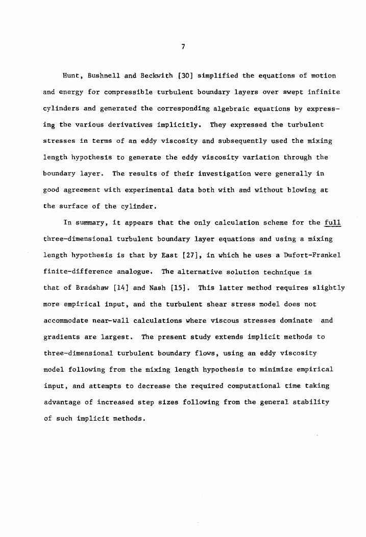
Hunt, Bushnell and Beckwith [30] simplified the equations of motion

and energy for compressible turbulent boundary layers over swept infinite

cylinders and generated the corresponding algebraic equations by express­

ing the various derivatives implicitly. They expressed the turbulent

stresses in terms of an eddy viscosity and subsequently used the mixing

length hypothesis to generate the eddy viscosity variation through the

boundary layer. The results of their investigation were generally in

good agreement with experimental data both with and without blowing at

the surface of the cylinder.

In summary, it appears that the only calculation scheme for the full

three-dimensional turbulent boundary layer equations and using a mixing

length hypothesis is that by East [27], in which he uses a Dufort-Frankel

finite-difference analogue. The alternative solution technique is

that of Bradshaw [14] and Nash [15]. This latter method requires slightly

more empirical input, and the turbulent shear stress model does not

accommodate near-wall calculations where viscous stresses dominate and

gradients are largest. The present study extends implicit methods to

three-dimensional turbulent boundary flows, using an eddy viscosity

model following from the mixing length hypothesis to minimize empirical

input, and attempts to decrease the required computational time taking

advantage of increased step sizes following from the general stability

of such implicit methods.

III. INVESTIGATION

An implicit finite-difference technique was incorporated to solve

the governing differential equations for a three-dimensional incompress-

ib1e turbulent boundary-layer flow. The difference equations were

written in such a manner as to form a set of quasi-linear algebraic

equations whose coefficients constituted a tridiagonal matrix. The

Thomas [31] algorithm was written to obtain the solution set, instead

of the time-consuming matrix inversion techniques. Finally an analysis

was undertaken to determine the stability and convergence of the finite-

difference equations.

A. The Governing Equations

The equations of motion and continuity which govern the unsteady

flow of an incompressible fluid are given by Hinze [4] as

aQ. -.J. = 0 ax

j

where

j=1,2,3

ClQi aQ. =_+......:.J.. ax. ax.

J 1

i=1,2,3 j=1,2,3

i=1,2,3 j=1,2,3

D and Dt is the substantial derivative.

(3.1)

(3.2)

To obtain a solution of these equations for turbulent flow, the

equations can be time smoothed and the resultant mean-flow equations

solved. One serious drawback of this approach is the introduction of

8

9

six additional unknowns in the form of apparent or Reynolds stresses.

The time-smoothing procedure is outlined in Hinze [4] and the resultant

governing equations, in the absence of body forces, are

DQi ap a - --+ (D - PQi'Qj') p Dt = - ax. ax. 11 j i

1 J

aQ. _.:1 = 0 ax.

J j=1,2,3

i=1,2,3 j=1,2,3

where the following substitutions were made

p = p + p'

(3.3)

(3.4)

with Q~ and pi representing the turbulent fluctuations of the velocity 1

and the pressure, respectively, and the overbar signifing the time-

average value.

According to Boussinesq's [4] hypothesis, the apparent "kinematic"

turbulent stresses can be expressed as functions of mean velocity

gradients and a scalar eddy viscosity as shown in Eq. 3.5.

- QiQj = £Dij i=1,2,3 j=1,2,3

With this hypothesis the equations of motion became

(3.5)

(3.6)

Equations 3.6 and 3.4 were reduced from 4 equations and 4 unknowns

to 3 equations and 3 unknowns by making the typical boundary-layer

assumptions for flow over a surface defined by the plane, Y = O. This

procedure is outlined in Schlichting [32] for two-dimensional flows and

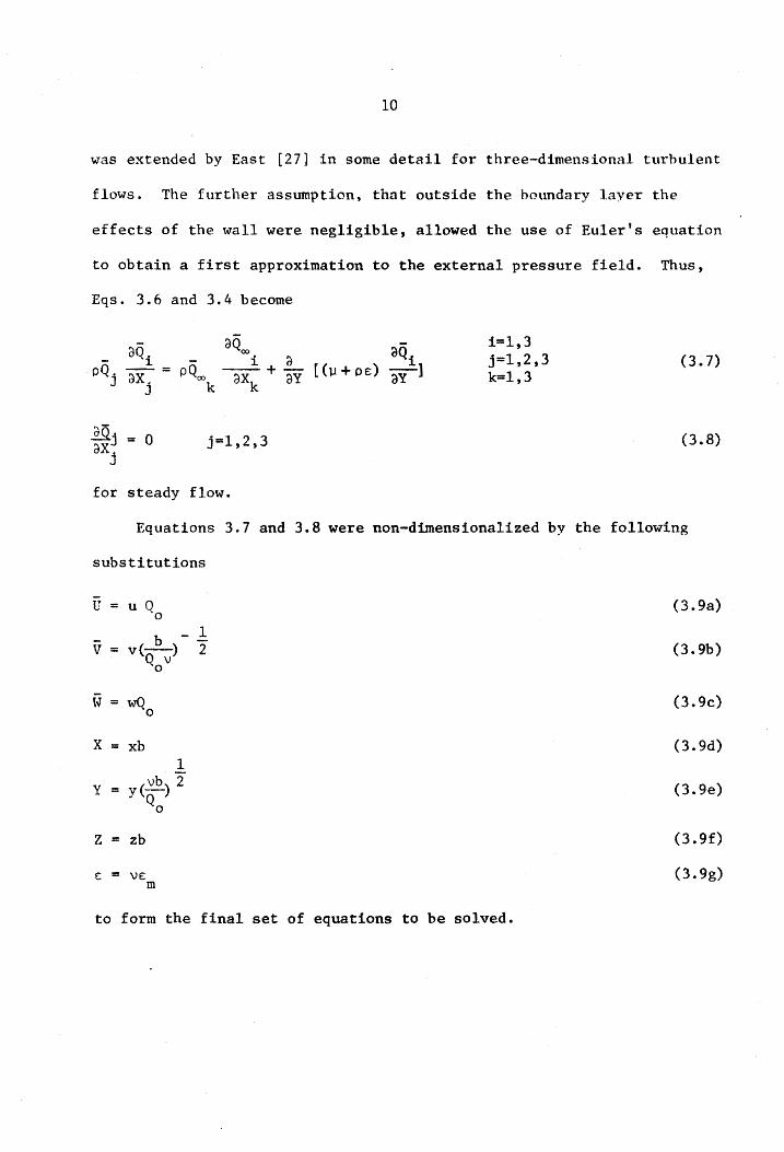
10

was extended by East [27] in some detail for three-dimensional turbulent

flows. The further assumption, that outside the boundary layer the

effects of the wall were negligible, allowed the use of Euler's equation

to obtain a first approximation to the external pressure field. Thus,

Eqs. 3.6 and 3.4 become

o j=l,2,3

for steady flow.

i=1,3 j=1,2,3 k=1,3

(3.7)

(3.8)

Equations 3.7 and 3.8 were non-dimensiona1ized by the following

substitutions

U = u Q o

b - 1. V = v(Q ,) 2

a

w = wQ o

x = xb 1

y = y(vb) 2" Qo

Z = zb

e: = 'VE: m

to form the final set of equations to be solved.

(3.9a)

(3.9b)

(3.9c)

(3.9d)

(3.ge)

(3.9f)

(3.9g)

11

uu + vu +wu = u u + w u + [(1 + E ) Uy1y x y z 00 oox 00 ooz m (3.l0a)

uw + vw + ww = uw +ww + [(1 + E ) w J x y z 00 oox 00 ooz m y y (3.l0b)

u +v + w = 0 x y z (3.l0c)

The subscripts x, y and z denote the partial derivative of a quantity,

for example: au - = u • dX x

By the nature of the boundary-layer approximations the problem was

reduced from a boundary-value problem in the three coordinate directions

to an initial-value problem with respect to the variables x and z and a

boundary-value problem with respect to y.

In some flow geometries a region of essentially two-dimensional flow

exists upstream of the three-dimensional flow field under consideration.

Thus to generate the initial values of u, v, and w for the x = 0 plane,

the momentum and continuity equations are easily simplified for a two-

dimensional turbulent boundary-layer flow and the resultant two-dimen-

ional solution can be used to initiate the three-dimensional solution.

The initial conditions on the z = 0 plane depend on the physical

flow circumstance to be studied. One class of three-dimensional boundary-

layer flows which is governed by Eqs. 3.10 is typified by flow over a

nearly-flat infinite swept wing. For this case, the derivatives with

respect to z are all identically zero with the proper choice of coordinate

system orientation, hence, eliminating the necessity for the z-direction

initial conditions. External boundary-layer flows over a flat plate

with an obstruction constitute another class of flows that may be

12

considered for solution. For the condition in which the obstruction is

a symmetrically shaped object, a plane of symmetry exists along the

stagnation streamline and becorr.es the initial condition fo~

the z-direction. For the case when the object is asymmetric, care must

be taken in generating the z-boundary condition because of the curvature

of the stagnation free-stream streamline. For the asymmetric circum-

stance a streamline-coordinate set would probably be more suitable.

Thus, the present investigation will be directed toward this second class

of flows, and specifically, those cases when the obstruction is symmetric.

On the plane of symmetry, or for two-dimensional flows, the equa-

tions of motion and continuity are

uu + vu = u u + [(1 + £ ) U y 1y x y 00 oox m (3.11a)

u + v + w = 0 x y z (3.llb)

and the z-momentum equation is identically equal to zero, which leaves

only 2 equations but 3 unknowns. To remedy this situation the z-momentum

equation was differentiated with respect to z and a third equation was

dW generated for the unknown az (which will be denoted as wz).

2 u(wz)x+ v(wZ) + (wz) (wz) = u (wzJ + (wz) + [(1 + £ )wz ]

'Y 00 x 00 m y y (3.12)

Equations 3.11 and 3.12 are the equations governing two-dimensional

and plane of symmetry turbulent boundary-layer flows and also form the

basis for generating the initial conditions for the three-dimensional

solution.

13

B. The Eddy-Viscosity Model

There are many eddy-viscosity models available in the literature

for two-dimensional boundary-layer flows. One such model that has

gained wide-spread usage was introduced by Prandtl [4]t who postulated

that the eddy viscosity be formed as a function of a mixing length

and a velocity gradient.

E: = R, 2 dU 8Y (3.13)

au The quantity ay can also be represented as a function of the magnitude

of the first rate-of-strain invariant [33)

(3.l4a)

when only the highest order terms are retained. consistent with the two-

dimensional boundary-layer approximations. Prandtl (see Goldstein [34])

extended the mixing length model to three-dimensional flows and developed

an expression for the corresponding eddy viscosity.

i=1,2.3 j=I.2,3 (3.15)

When the usual boundary-layer approximations are applied to the rate-of-

strain invariant for three-dimensional boundary layers, the expression

for the eddy viscosity model becomes

1

e:: = t 2[(U )2 + (W)2]2 y Y

Non-dimensionally, this expression is written as 1

= L2(u )2 + (w)2]2 Em y y

(3.l6a)

(3.16b)

14

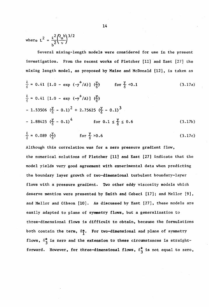
2 i2~ b)3/2 where L =--~ b2 v

Several mixing-length models were considered for use in the present

investigation. From the recent works of Pletcher [11] and East [27] the

mixing length model, as proposed by Maise and McDonald [12], is taken as

£ + ~ 6 = 0.41 [1.0 - exp (-y /A)] (0) for t <0.1 (3.l7a)

I = 0.41 [1.0 - exp (-Y+/A)] <f)

- 1.53506 (! - 0.1)2 + 2.75625 <t - 0.1)3

- 1.88425 <! - 0.1)4 for 0.1 ! t ! 0.6 (3.l7b)

~ = 0.089 (r) for t >0.6 (3.17c)

Although this correlation was for a zero pressure gradient flow,

the numerical solutions of Pletcher [11] and East [27] indicate that the

model yields very good agreement with experimental data when predicting

the boundary layer growth of two-dimensional turbulent boundary-layer

flows with a pressure gradient. Two other eddy viscosity models which

deserve mention were presented by Smith and Cebeci [17]; and Mellor [9],

and Mellor and Gibson [10]. As discussed by East [27], these models are

easily adapted to plane of symmetry flows, but a generalization to

three-dimensional flows is difficult to obtain, because the formulations

both contain the term, 0t. For two-dimensional and plane of symmetry

flows, 0; is zero and the extension to these circumstances is straight­

forward. However, for three-dimensional flows, 0; is not equal to zero,

15

and a question arises whether to use at only or replace the terms

containing at by some yet to be determined combination of o! and o~.

The value of A in Eqs. 3.17 was taken by the previous investigators

as 26 after van Driest [7]. However. van Driest determined this value

by obtaining a best fit to Laufer's data [35] which generally followed

the law of the wall with the following constants

+ u 1 In y+ = 0.40 + 5.24 (3.18)

For equilibrium turbulent boundary-layer flows in two dimensions, Coles

(36] studied some 500 profiles and suggested that the law of the wall

constants should be as in Eq. 3.19.

+ 1- + u = O. 41 In y + 5. 0 (3.19)

To obtain a value of the parameter A, consistent with this set of

constants, a procedure analogous to van Driest's was followed and the

law of the wall formulation was closely approximated as

+ 1 + u = 0.41 In y + 5.07 (3.20)

for a value of A of 25. This value was considered acceptable since

van Driest noted that to fit Nikuradse's data, the parameter t A, was

equal to 27 instead of 26.

c. Finite Difference Formulation

A Crank-Nicholson [37] implicit finite difference scheme was

utilized for the following reasons:

(i) For laminar two-dimensional boundary-layer flows the

resultant equations have been shown to be stable and

16

convergent by FlUgge-Lotz and Blattner [25].

(ii) The truncation errors are of order (fix); (6y)2 and (Az)2

which would minimize the computer time because of the

larger step sizes that can be taken.

(iii) If the finite difference equations are written in

such a manner as to form a tridiagonal matrix of coefficients,

the solution of the difference equations does not require

matrix inversion. Instead a simple algorithm can be written

to obtain the solution.

1. Two-Dimensional and Plane of Symmetry Formulation

Figure 3.1 shows the grid construction used to generate the finite

difference approximations for the two-dimensional and plane of symmetry

flows. The difference approximations shown below are given for any

1 variable H about the point (1 + 2,j,k). The equations were written for

a variable y-grid spacing allowing more dense node locations in regions

of large gradients and fewer locations in regions of small gradients.

Terms appearing in Eqs. 3.1la and 3.12 are given as

(H) H(i+l,j,k) - H(i,j,k) 1 (H) (AX) 2 x = 6x - 24 xxx

(H) = 2(A1 +6 ) {~Y-[(H(i,j+l,k) - H(i,j,k)

y y+ y- y+ 6Y+

+ H(i+1,j+l,k) - H(i+l,j,k» + ~(H(i,j,k) y-

- H(i,j-1,k) + H(1+1,j,k) - H(i+l,j-l,k»]}

1 1 2 - -6(H) (6y+)(6Y ) - -8 (H) (6.x) yyy - xxy

(3.21a)

(3.21b)

17

i,j+l,k) ( ;+1 ,j+1 ,k)

l1y -

(i,j,k) (;+1,j,k)

b.y +

(i,j-l,k) •

b.x ------......... 1 (i+1,j-1,k)

Fig. 3.1 Two-Dimensional Finite Difference Grid.

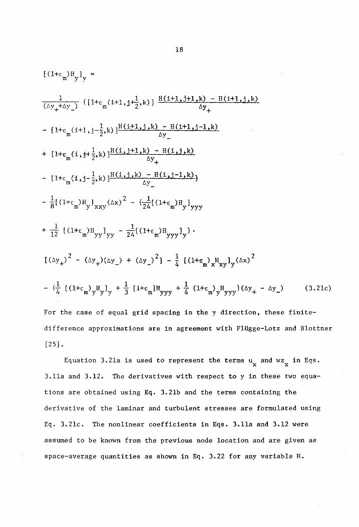
[(l+E ) H] = m y y

IS

1 {[1+Em(i+1,j~2,k)] H(i+1,j+1,k) - H(i+l,j,k) (6y++6y_) 6y+

[ 1+ ('+1' _! k) ]H (i+l ,j ,k) - H(i+l ,j -1 ,k) - 8 m 1 ,J 2' 6y_

+ [1+£ (i,j-f 4,k) ]H(i,j+l,k~ - H(i,j ,k) m y+

_ [1+8 (1 ._! k) ]H(i,j ,k) - H(i,j-l,k)} m ,] 2' t.y_

- -Sl[(l+s )H] (6x)2 - {241 [(1+8 )H ] m y xxy m y yyy

- {41 [(l+E ) H] + 1 [1+8]H + 14 (1+£ ) H }(6y+ - 6y ) m y y y 3 m yyy m y yyy -

(3.21c)

For the case of equal grid spacing in the y direction, these finite-

difference approximations are in agreement with F1Ugge-Lotz and B10ttner

[25] •

Equation 3.2la is used to represent the terms u and wz in Eqs. x x

3.l1a and 3.12. The derivatives with respect to y in these two equa-

tions are obtained using Eq. 3.2lb and the terms containing the

derivative of the laminar and turbulent stresses are formulated using

Eq. 3.21c. The nonlinear coefficients in Eqs. 3.11a and 3.12 were

assumed to be known from the previous node location and are given as

space-average quantities as shown in Eq. 3.22 for any variable H.

H = H(i+l,j,k) +H(i,j,k) 2

19

(3.22)

Thus, H(i+l,j,k) is equal to H(i,j,k) as a first approximation and an

iterative procedure is used to determine successively better approxi-

mations to H(i+l,j,k). The details of this iterative scheme are given

in a later section.

To simplify the resultant difference equations the following

definitions are introduced.

r l = v(l~X_)6x

2u(6y+) (6y+ + 6y_) (3.23a)

r 2 V (6y+6x 2U(Ay_) (6y+ + 6y_) (3.23b)

r3 = (wz)6x

2\1 (3.23c)

(l+£m(i~l,j+~,k» Ax sl = { 3

u (6Y+) (AY+ + 6Y_) (3.23d)

(l+£m(i+l,j-~,k» { 6x } s2 =

u (8Y_) (6Y+ + 6y_)

(l+£m(i,j+~,k» 6x fly _) } s3 u {(8Y+) (fly+ +

(3.23e)

(3.23f)

1 (l+E:m(i,j-Z,k» 6x

s4 = { } u (6y_) (6y+ + 6y_)

(3.23g)

With this notation the difference approximations for the momentum

equations become

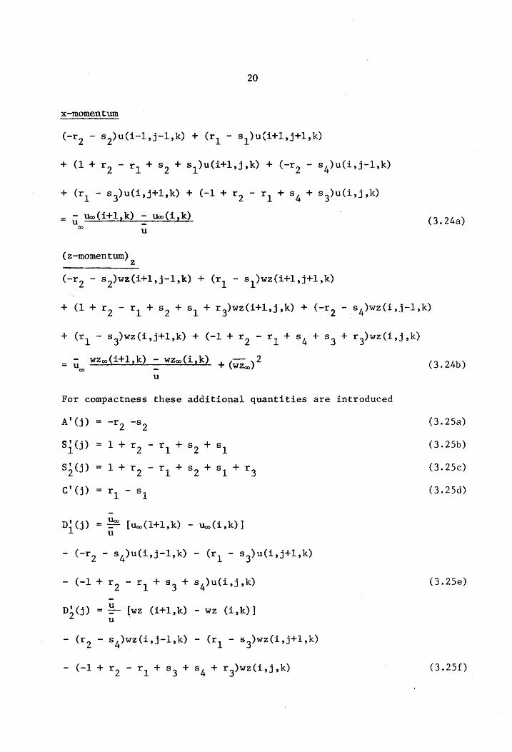
x-momentum

= ~ Uro(i+l,k) : Uoo(i,k} 00

(z-momentum) z

u

20

(-r2 - 8 2)wz(i+1,j-1,k) + (r1 - 81)wz(i+I,j+l,k)

+ (r1 - 8 3)wz(i,j+1,k) + (-1 + r 2 - r 1 + 8 4 + s3 + r 3)wz(i,j,k)

= u wzoo(i+l,k) : wZoo(i,k) + (wzoo) 2

00

u

For compactness these additional quantities are introduced

A' (j) = -r2 -82

Si(j) = 1 + r 2 - r 1 + s2 + 8 1

82 (j) = 1 + r2 - r + s2 + sl + r 3 1

c' (j) = r 1 - sl

= Uoo [Uoo(l+l,k) - Uoo(i,k)] u

D2(j) = ~ ~wz (i+l,k) - wz (i,k)] u

(3.24a)

(3.24b)

(3.25a)

(3.25b)

(3.25c)

(3.25d)

(3.25e)

(3.25f)

21

The resultant algebraic equations to be solved are shown below.

x-momentum

A'{j) u(i+1,j-1,k) + Si(j) u(i+l,j,k)

+ C' (j) u{i+l,j+l,k) = D' (j) 1

(z-momentum)

j = 2,3 ••• n

A'(j) wz(i+1,j-l,k) + Si(j) wz(i+l,j,k)

+ C'(j) wz(i+l,j+l,k) = Di(j) j = 2,3 .... n

(3.26a)

(3.26b)

Note that both Eqs. 3.26a and 3.26b have a matrix of coefficients

that is tridiagonal (i.e., the matrix contains non-zero elements only on

the principal diagonal and the two diagonals to either side). The

details of the method of solution will be discussed in a later section

of this chapter.

Two finite-difference formulations of the continuity equation

(Eq. 3.11b) are posed for use in the solution. Method I evaluates the

derivatives at the point (i+l,j-~,k) on Fig. 3.1 and utilizes a backward

difference scheme for the x derivative.

1 v = -- [v(i+l,j,k) - v(i+1,j-l,k)] y /1y

1 2 - 24 (v)yyy(~y_)

1 ux = 2t.x (u(i+l,j ,k) + u(i+l,j-l,k) - u(i,j ,k)

- u(i,j-1,k)] + !2 (u) bx xx

112 w = -2 [wz(i+l,j,k) + wz(i+l,j-l,k)] - -8 u (6y) z yy -

(3.27a)

(3.27b)

(3.27c)

22

Method II evaluates the derivatives at the point (i+~,j-~,k) on Fig. 3.1

so that the resultant finite difference approximations are

1 (v)y = 2~y [v(i+l,j,k) + v(i,j,k) - v(l+l,j-l,k)

- v(i,j-l,k)]

1 (v) (~x)2 1 ( ) (~y_)2 8 xxy - 24 v yyy (3.28a)

1 (u) = -2-- [u(i+l,j,k) + u(i+l,j-l,k) - u(i,j,k) x ~x

1 2 1 2 - u(i J' -1 k)] - - (u) (~x) - - (u) (~y ) " 24 xxx 8 xyy - (3.28b)

1 Wz 4 [wz(i+l,j,k) + wz(i,j,k) + wz(i+l,j-l,k) + wz(i,j-l,k)]

1 2 1 2 - -S u (~x) - 8- u (~y) xx yy

(3.2Sc)

Thus, the continuity equation is written in the following two forms:

Method I

v(i+l,j,k) = v(i+l,j-l,k) - ~2Y- [u(i+l,j,k) ~x

+ u(i+l,j-l,k) - u(i,j,k) - u (i,j-l,k)] - ~ [wz(i+l,j,k)

+ wz(i+l,j-l,k)J

Hethod II

v(i+l,j,k) = v(i+l,j-l,k) + v(i,j-l,k) - v(i,j,k)

_ ily_ [u(i+l,j,k) + u(i+l,j-l,k) - u(i,j,k) - u(i,j-l,k)]

x

- ~~- [wz(i,j,k) + wz(i,j-l,k) + wz(i+l,j,k) + wz(i+l,j-l,k)]

(3.29a)

(3.29b)

The choice of which continuity expression to use was the subject of a

brief analysis and the findings will be presented in a later section.

23

2. Three-Dimensional Formulation

Figure 3.2 shows the grid used to model the finite differences for

the three-dimensional problem. The difference formulations are shown

below using a Crank-Nicholson finite difference scheme extended to three

dimensions about the point (i+~,j,k-~) for any variab1e t H. Again a

variable grid spacing in the y direction was used. Typical derivative

terms appearing in Eqs. 3.10a and 3.10b are given as

Hx = 2!X [H(i+1,j,k) + H(i+1,j,k-1) - H(i,j,k)

- H(i,j,k-l)] - ~ (H)xzz(8Z)2 - 2!(H)xxx(8X)2

Hz = 2!z[H(i+l,j,k) + H{i,j,k) - H(i+1,j,k-1)

H 4(8 1+ 8 ) {(~Y-)[H(i,j+1,k) - H(i,j,k) Y y+ y_ uy+

+ H(i,j+l,k-1) - H(i,j,k-l) + H(i+1,j+l,k)

- H(i+1,j,k) + H(i+1,j+l,k-l) - H(i+1,j,k-l)]

+ (~Y+)[H(l,j,k) - H(i,j-1,k) + H(l,j,k-l) - H(i,j-l,k-1) y-

+ H(i+1,j,k) - H(i+l,j-l,k) + H(i+1,j,k-1) - H(i+1,j-1,k-l)]}

1 ( ) ) ( ) 1 2 1 ( (8Z) 2 - 6 H yyy (8y+ 8y_ - 8 (H)yxx (8X) - 8 H)yzz

[(1+£ )H J = m y y

1 {[l+E (i+1 "+! k)]H(1+1,j+1,k) - H(i+l,j,k) 2(8Y+ + 8y_) m ,] 2' l1y+

(3.30a)

(3.30b)

(3.30c)

24

(;+1 ,j+l ,k-l)

I I J

I I (i+l~j,k-l) .... I', I '

I /'

/' J

,,/'/' I

/'(i,j,k-l) : (; + 1 ,j -1 ,k -1 ) ....

", ...

Fig. 3.2 Three-Dimensional Finite Difference Grid.

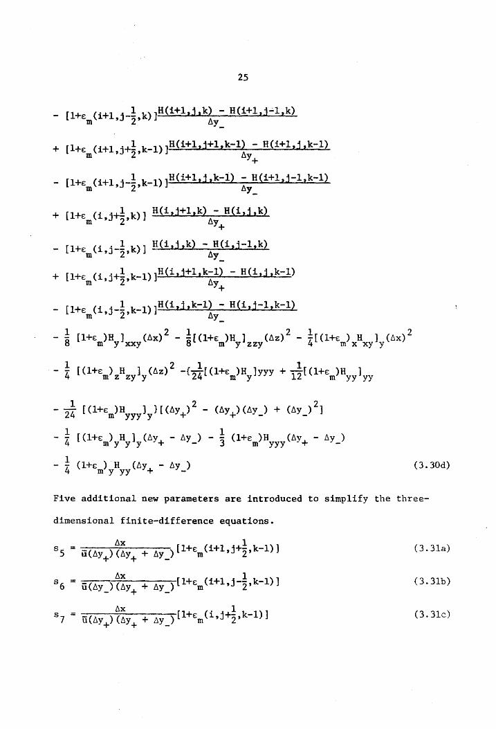
25

- [1+ (1+1 j_! k)]H(1+1,j,k) -H(i+1Jj~1,k) £m '2' 6y_

+ [1+£ (i+1 .+! k_1)]H(i+1 zj+1,k-l) - H{i+l,j,k-1) m .,J 2' 6y

+

_ [1+£ (i+1 o_! k_1)]H(i+1,j zk-1) - H(i+1 zj-1 zk-1) m ,J 2' Ily_

+ [1+£ (1 ·+1 k)] H(i,j+l,k) - H(i,j,k) m ,J 2' 6y

+

- [1+£ (i ._! k)] H(i,jzk) - H(i,j-1,k) m ,J 2' Ily_

+ [1+£ (i .+! k_l)]H(i,j+l,k-l) - H(i,j,k-l) m ,J 2' Ily

+

[1+£ (i ._! k_l)]H(i,j zk-1) - H(i z1-1,k-l) m ,J 2' 6y_

1 [1+£ )H] (6x)2 - !S[(l+£ )H] (llz)2 - !4[(1+£ ) H ] (6x)2 8 m y xxy m y zzy m x xy y

- !4 [(1+£ ) H 1 (6z)2 -{24l [(1+£ )H ]yyy + 112[(1+£)H ] m z zy y m y m yy yy

122 - 24 [(l+£)H ] }[(Ily+) - (lly+)(lly_) + (6y_) ] m yyy y

- !4 [(1+£ ) H ] (6y+ - 6y ) - !3 (l+£)H (6y+ - 6y ) m y y y - m yyy -

- -41 (1+£ ) H (6y+ - 6y ) m y yy - (3.30d)

Five additional new parameters are introduced to simplify the three-

dimensional finite-difference equations.

6x 1 Ss = u(6y+) (8Y+ + 6y_) [1+£m(i+1,j+2,k-1)] (3.3la)

6x 1 8 6 = u(6y_) (6Y+ + 6y_) [1+£m(i+1,j-2,k-l)] (3.31b)

8 7 = U(AY+)~~Y+ + Ay_)[l+Em(i.j~.k-l)l (3.31c)

t = wllx ii6z

26

(3.31d)

(3.3le)

where the notation of the overbar is changed from the definition given

in Eq. 3.22 to

- 1 H = 4 [H(i+1,j,k) + H(i+1,j,k-1) + H(i,j.k) + H(i,j,k-1)] (3.32)

~.vith the use of Eqs. 3.30, 3.31, and 3.22 (with the noted change in the

definition of H) and linearizing the resultant equations, with the same

procedure as outlined for the two-dimensional equations the finite

difference approximations for the three-dimensional turbulent boundary-

layer equations become

x-momentum

+ (-r2 - s6)u(i+l,j-l,k-1) + (ri

- sS)u(i+l,j+l,k-l)

+ (r1 - s7)u(i,j+l,k-1) + (-1 + r2

- r l + 8 a + 87

- t)u(i,j,k-l)

Uoo = :-[Uoo(i+1,k) - u (i,k) + uoo(i+l,k-l) - u (i,k-I)] u 00 00

+ ~OO~x[Uoo(i+l,k) + u (i,k) - u (1+1,k-l) u (i,k-I)] u~z 00 00 00

(3.33a)

27

z-rnomentum

(-r2

- s2)w(i+l,j-l t k) + (r1 - sl) w(i+l,j+1,k)

+ (1 + r 2 - r 1 + s2 + sl + t)w(i+1,j,k) + (-r2 - s4)w{i,j-l,k)

+ (-r2 - s6)w(i+1,j-1,k-1) + (r1

- s5)w(i+l,j+l,k-1)

+ (1 + r 2 - r 1 + s6 + s5 - t)w(i+l,j,k-l) + (-r2 - sa)w(i,j-l,k-1)

-= ~[woo(i+l,k)-woo(i,k) + woo (i+1,k-1-woo{i,k-l)]

u

+ ~OO~x[w (i+1,k) - w (i+l,k-1) + w (i,k) - w (i,k-1)] uAz 00 00 00 00

(3.33b)

The definition of A'(j) and C'(j) are retained (see Eqs. 3.25a and

3.Z5d) and the additional variables S3(j), S4(j), D3(j) and D4(j) were

defined to cast the equations of motion into the general tridiagonal form.

S;(j) = S4(j) = r Z - r l + s2 + sl + t + 1 (3.34a)

D3(j) = ~[Uoo(i+l,k) - Uoo(i,k} + Uoo(i+1,k-1) - Uoo(i,k-1)] u

+ W~b.x[Uoo(i+1,k) - Uoo(i+1,k-1) + Uoo{i,k) - uoo (i,k-1)] UuZ

+ (-1 + r Z - r 1 + s4 + 8 3 + t)u(i,j,k) + (-r2 - s6)u(i+1,j-1,k-1)

+ (r1 - s5)u(i+1,j+1,k-1) + (1 + r 2 - r 1 + 8 6 + 8 5 - t) u(i+l,j,k-l)

+ (-1 + r 2 - r 1 + sa + s7 - t)u(i,j,k-l)} (3.34b)

28

D4'(j) = ~[w (i+ltk) - w (i,k) + w (i+l,k-1) - woo(i,k-l)] u 00 00 00 .

+ ~oo6Xrwoo(i+l,k) - woo(i+l,k-l) + woo(i,k) - woo (i,k-1)] u6z .

+ (-1 + r 2 - r l + s4 + s3 + t)w(i,j,k) + (-r2 - s6)w(i+1,j-1,k-1)

+ (r l - s5)w(i+l,j+l,k-l) + (1 + r 2 - r l + 8 6 + s5 - t)w(i+1,j,k-l)

+ (-1 + r 2 - r 1 + s8 + 87

- t)w(i,j,k-l)} (3.34c)

Thus the momentum equations are written as

x-momentum

A'(j)u(i+l,j-1,k) + S)(j)u(i+l,j,k)

+ C'(j) (i+1,j+l,k) = D)(j) j = 2,3, ••• n (3.35a)

z-momentum

A' (j)w(i+1,j-l,k) + S;'(j)w(i+l,j,k)

+ C'(j)w(i+1,j+l,k) = D4(j) j = 2,3, ••• n (3.35b)

Equations 3.35 are the final form of the momentum equations that are

solved in the three-dimensional turbulent boundary layer problem posed

in this investigation.

Again an adequate finite difference representation of the continuity

equation had to be formulated to complete the set of governing equations.

Analogous to the two-dimensional problem formulation, two methods of

approximating the continuity equation are proposed.

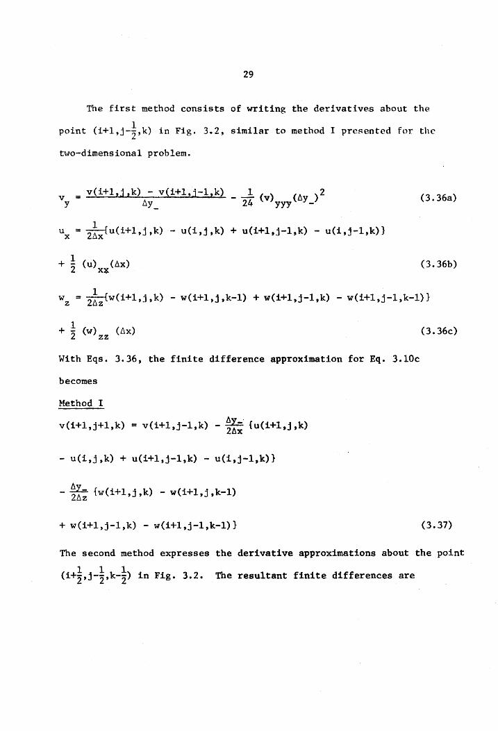
29

The first method consists of writing the derivatives about the

point (i+l,j-~,k) in Fig. 3.2, similar to method I presented for the

tl-lo-dimensional problem.

v = v(i+l,j,k) - v(i+l,j-l,k) 1 2 y 6y _ - 24 (v)yyy (6y_)

Ux = 2!x(U(i+l,j,k) - u(i,j,k) + u(i+l,j-l,k) - u(i,j-l,k)}

1 + -2 (u) (l\x) x¥

(3.36a)

(3.36b)

Wz = 2~z(W(i+l,j,k) - w(i+l,j,k-l) + w(i+l,j-l,k) - w(i+l,j-l,k-l)}

+ !2 (w) (llx) zz

With Eqs. 3.36, the finite difference approximation for Eq. 3.10c

becomes

Method I

~ v(i+l,j+l,k) = v(i+l,j-l,k) - 26; {u(i+l,j,k)

- u(i,j,k) + u(i+l,j-l,k) - u(i,j-l,k)}

- ~1; {w(i+l,j,k) - w(i+l,j,k-l)

+ w(i+l,j-l,k) - w(i+l,j-l,k-l)}

(3.36c)

(3.37)

The second method expresses the derivative approximations about the point

III (1+2,j-i,k-2) in Fig. 3.2. The resultant finite differences are

30

1 U x = 4~x [u(i+l,j,k) - u(i,j,k) + u(i+l,j,k-l) - u(i,j,k-l)

+ u(i+l,j-l,k) - u(i,j-l,k) + u(i+l,j-l,k-l) - u(i,j-l,k-l)]

Vy D 4~i_ [v(i+l,j,k) - v(i+l,j-l,k) + v(i,j,k) - v(i,j-l,k)

+ v(i+l,j,k-l) - v(i+l,j-l,k-l) + v(i,j,k-l) - v(i,j-l,k-l)]

(3.38a)

(3.38b)

Wz = 4~z [w(i+l,j,k) - w(i+l,j,k-l) + w(i+l,j-l,k) - w(i+l,j-l,k-l)

+ w(i,j,k) - w(i,j,k-l) + w(i,j-l,k) - w(i,j-l,k-l)]

(3.38c)

The resultant continuity expression is shown below for this set of

finite d·ifference approximations.

Method II

v(i+l,j,k) = v(i+l,j-l,k) + v(i+l,j-l,k-l) + v(i,j-l,k)

+ v(i,j-l,k-l) - v(1+1,j,k-l) - v(i,j,k) - v(i,j,k-l)

- ~-[U(i+l,j,k) - u(i,j,k) + u(i+l,j-l,k) - u(i,j-l,k)

+ u(i+l,j,k-l) - u(i,j,k-l) + u(i+l,j-l,k-l) - u(i,j-l,k-l)]

- ~~- [w(i+l,j,k) - w(i+l,j,k-l) + w(i+l,j-l,k) - w(i+l,j-l,k-l)

+ w(i,j,k) - w(i,j,k-l) + w(i,j-l,k) - w(i,j-l,k-l)] (3.39)

Equations 3.37 and 3.39 constitute the proposed forms of the

continuity equation to be used in the three-dimensional turbulent

boundary-layer flow solution. A discussion as to the final choice

31

of form will be found in a later section of this chapter.

Finally, the consequences of the linearization technique used to

develop the tridiagonal finite difference forms of the equations of

motion will also be discussed in a later section of this chapter.

D. Generation of Boundary Conditions and Initial Conditions

Two three-dimensional flow geometries were investigated numerically

and the results were compared to the corresponding experimental data

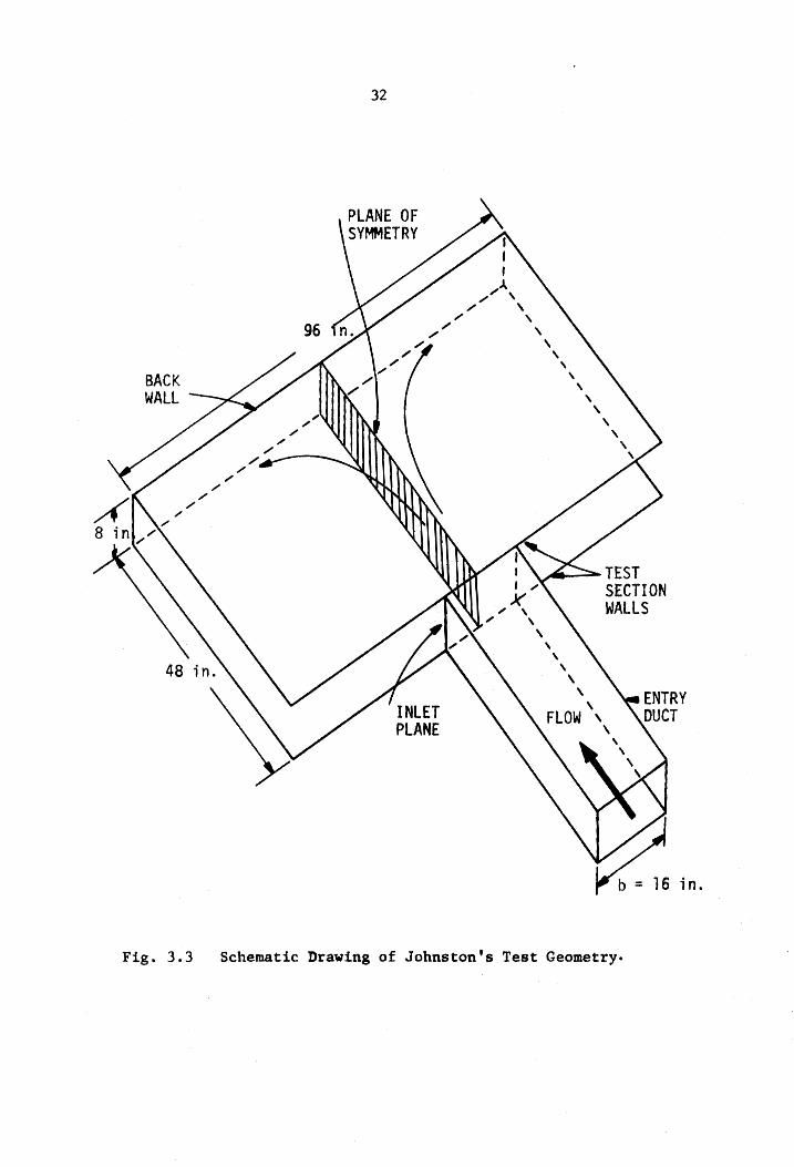
presented by Johnston [28] and Hornung and Joubert [29]. Johnston's

experimental apparatus consisted of a rectangular inlet duct from which

the issuing jet impinged on an end wall 48 in. from the outlet of the

channel. The jet was confined on the top and bottom by flat surfaces,

and the boundary layer which developed on the floor of the test section

was probed. A schematic of this geometry is shown in Fig. 3.3. Hornung

and Joubert experimentally investigated the boundary layer growth on the

floor of the large test section in which a vertical airfoil with a

cylindrical front was placed perpendicular to the flow direction as

sholvn in Fig. 3.4. The lead-in section was about 17 ft from the center

of the cylinder and the channel was slightly divergent.

The initial condition and boundary conditions were generated in the

same manner for both three-dimensional geometries as described below.

(1) A two-dimensional zero pressure g~adient turbulent

boundary layer was developed from the leading edge of a

flat plate with the following initial conditions as pre­

scribed by Wu [38]

32

Fig. 3.3 Schematic Drawing of Johnston's Test Geometry.

----I ...... FLOW

Fig. 3.4

22 in. 0

17 ft. ..01

Schematic Drawing of Hornung and Joubert's Tast Geometry.

w w

34

u(o,y,z) = u (o,z) co

(3.40a)

v(o,y,z) =·w(o,y,z) = wz(o,y,z) = 0 (3.40b)

u(x,o,z) v(x,o,z) = w(x,o,z) = wz(x,o,z) = 0 (3.40c)

u(x,o,z) = u (x,o ,z) (3.40d) 00

w(x,o,o) = wz(x,o ,0) = 0 (3.40e)

This procedure could be modified for pressure gradient flm.;rs

if the pressure gradient of the inlet channel were known.

However, for the cases studied either the pressure gradient

was nearly zero (Johnston's experiment) or it was not specified

(Hornung and Joubert's experiment).

(2) At some distance down the flat plate the plane of

symmetry solution was initiated using the previously

determined two-dimensional profile. To proceed from this

point the pressure gradient was prescribed by the potential

flow solution for the given geometry.

(3) The plane of symmetry solution was continued until a

match point was reached where the resultant solution was

compared to the available experimental data.

(4) The lengths of the two-dimensional solution and the

plane-of-symmetry solution were adjusted appropriately and

steps (1), (2), and (3) were repeated until the desired fit

was obtained. For the Johnston geometry the match point was

at station D-8 as shown in Fig. 3.5. This point also

corresponded to the location at which the plane of symmetry

solution was started, since this match point was in a

35

5 5

2.5 2.5

1'1

'" '" BACK WALL ~, j

~ M

1 0 ) I N

Xl 0 ..,~

I N 1..0

X2 0 ~I"-

) I N

2 0

( I N

X3 0 !1t-I N 1..0

X4 0 i-I--

J I N

3 -0-0-0-0-0-0-0-

I I I I t N

( X5 -0-0-1-0-1-0-0

I I I I I N 1..0

X6 -0-0-1-0-1-0-0-I-r--I I I I I N

4 -0-0-1-0 -1-0-0-I N

45 in. X7 0 -l"-

I N 1..0

X8 1 0 -l""-

) I N

5 0

t , M I

X9 0 t-- 1..0 ~ I M ,

6 0

I M

X10 0 -t-- 1..0

I (V) I 7 0

J xt

) 1..0

I

\ ~L z

I- 8 -0 .. j 0 ... 0- -t--

I 01 I M A BCDEF G t

I ENTRY I DUCT

- "'""'- --FLOW t

36

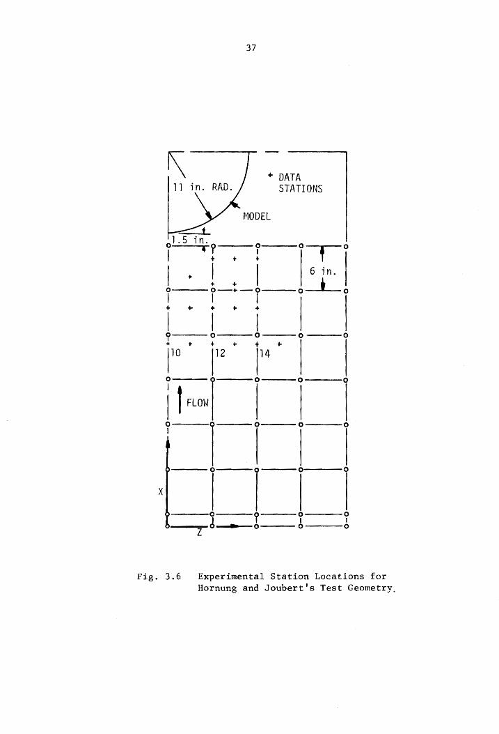
region far enough from the end wall so that a fully two­

dimensional profile could be assumed. For the Hornung and

Joubert geometry (see Fig. 3.6) the match point corresponded

to station 10 at which there were strong three-dimensional

effects. Thus, the plane of symmetry solution had to be

initiated at some point upstream where the three-dimensional

effects were negligible.

(5) After an adequate fit was obtained by steps (1) - (4)

at the match point, the complete three-dimensional solution

was obtained where the appropriate two-dimensional profile

was used as the x-direction initial condition, and the plane

of symmetry solution was generated simultaneously to provide

the initial conditions in the z-direction for the full three­

dimensional solution.

Two modifications were introduced when beginning the full three­

dimensional solution. Instead of assuming wand wz equal to zero as

provided by the two-dimensional solution, these quantities were assumed

to have the corresponding free-stream values which were considered to

more accurately represent these profiles. Also, the u-profile was

proportionally weighted along the X=O plane to insure that the resultant

profiles matched at the boundary layer edge with the potential flow

solution off the plane of symmetry. This procedure did, however, retain

the general shape of the profile off the plane of symmetry when compared

to the profile on the plane of symmetry at the match point.

0,·5

I

f +

0

I + +

I 0 I + ..

1

10

37

0 I

+ ...

+ + 0-"-0 I I + t +

I I 0 0 ... + +

+ DATA STATIONS

0 , 6 in.

0 I

0 .. 112 114

0

0

0

I f FLOW I 0 0 0

0 I

X

Fig. 3.6

I 0 0 0

0

I 0 0

0 Y 0 0

J I I

Z .. 0 0 0

Experimental Station Locations for Hornung and Joubert's Test Geometry.

38

Certain circumstances can occur for which the assumption of a zero

pressure gradient inlet section may have questionable validity. Thus,

the program was sufficiently generalized to allow a profile to be read in

to initiate either a two- or three-dimensional solution. These input

profiles can be obtained from a variety of sources such as a known

analytical solution, experimental correlations typified by the wall-wake

formulation [39], curve fits to experimental data, or a two-dimensional

pressure gradient solution previously obtained from the program itself.

As mentioned previously the pressure gradients were generated for

the three-dimensional flow solution from potential flow theory. Milne-

Thompson [40] and Pai [41] have detailed derivations for the impinging

jets problem which are applicable to the Johnston geometry. Their

results were non-dimensionalized as set forth in Eq. 3.9, where Q was o

equal to the velocity of the jet and b was equal to the width of the

jet at an infinite distance from the end wall. The resultant equations

are

F = 0 = - n (x - A*) - ! ~n[(I+Uoo)~ + Woo~] - 2! tan-l 2 2uoo 2 b 2 (l-u) + w l-u - w

00 00 00 00 (3.4la)

G = 0 I (1-woo)2 + U00

2 1 -1 2woo = - n z - '2 Q,n[(1+W00)2 + u002J + '2 tan l-Uoo2 - w002 (3.4lb)

where A* is a convenient distance that the origin was shifted along the

x axis. Equation 3.4lb was differentiated with respect to z and the

following expression was obtained for wz on the plane of symmetry

1T 4 wz = 4[1 - u~x,l (3.4Ic)

Unfortunately, Uoo and Woo could not be expressed explicitly in terms of

x and z. Thus, an extension of the Newton-Raphson method (see Traub [42])

39

was used to solve the simultaneous equations for Uoo

and Woo at each x

and z location. The potential flow solution for Hornung and Joubert's

geometry was taken as that of a uniform flow approaching a right

circular cylinder. The expressions for the velocities were non-

dimensionalized such that Q was the velocity of the uniform stream at o

an infinite distance from the cylinder and b was equal to the radius of

the cylinder. Again A* shifted the origin along the x axis.

(3.42a)

1 2 (A* - x) z . A* 2 2 2

b [(b" - x) + z ] (3.42b)

and on the plane of symmetry

wz 2 = -----(A* _ x)3 b

(3.42c)

E. Solution Technique

Equations 3.26 and 3.35 can be represented in a general tridiagonal

system of n - 1 equations in the form

Si(2)H(2) + C'(2)H(3) = D~(2) (3.43a)

A'(j)H(j-1) + Si(j)H(j) + C'(j)H(j+l) = D~{j) j = 3,4, ••• n -1 (3.43b)

At (n)H(n-l) + S! (n) = n'.' (n) 1 1

(3.43c)

for i = 1, 2, 3, 4 depending on the desired equation of motion to be

solved, and H(j) is a dummy variable which correspondingly becomes

40

u(i+l,j ,k), w'z(i+l,j ,k) u(i+l,j ,k) or w(i+l,j ,k).

The variable D',' (j) is introduced to more clearly show the nature of the ~

tridiagonal scheme D~(j) can be related to D~(j) as follows

D',' (2) = D! (2) - A(2)H(1) (3.44a) ~ 1.

D'.' (j) = Di(j) j = 3,4, ••• n - 1 (3.44b) 1.

nt.'(n) = Di(n) - A(n)H(n+l) (3.44c) ~

,-;rhere the following equivalences are applied

u (i,k) = u(i,n+1,k) co

w (i,k) = w(i,n+l,k) co

wz (i,k) = wz(i,n+l,k) co

Ames [31] outlines the use of the Thomas algorithm and a similar

procedure is used in this investigation. To begin the solution, a

Gaussian elimination was applied to Eqs. 3.43 to transform the matrix

into an upper bidiagonal form.

(3.45a)

j = 3,4, ••• n-l (3.45b)

H(n) = Fi(n) (3.45c)

for i = 1, 2, 3, 4 and the coefficients Ei(j) and Fi(j) were calculated

using the following recurrence formulae

E,(2) = C'(2) ~ Si (2)

(3.46a)

Fi(Z) D'.' (2)

1. = --:-~:-Si (2)

(3.46b)

41

j = 3,4 • •• n (3.46c)

j = 3,4 ••• n (3.46d)

where C'(n) = 0 by Eq. 3.43c. From Eq. 3.45c, H(n) ~as determined and

by successive substitutions into Eq. 3.47 below the remaining values of

H(j) were obtained.

j = n-l, n-2 ... 2 (3.47)

This method of solution was far superior to matrix inversion techniques

because of the great reduction in the number of calculations necessary

to solve the large system of equations.

When the finite difference equations were developed, the quantities

- - 1 1 u, v, w, WZ, £m(i+l,j+Z,k) and £m(i+l,j-2,k) were assumed to be known in

order to linearize the equations. Since all of the quantities are

functions of the variables to be determined at the new location an

iterative procedure had to be followed when solving the finite difference

equations at each new x and z location.

i) The velocity profiles at station (i,j,k) were projected

forward to station (i+l,j,k) for all j and k.

ii) The finite difference equations were solved and a first

approximation to the desired velocity profiles was ob­

tained at station (i+l,j,k) for each j.

iii) The results of step (ii) were used to generate new

coefficients for the finite difference equations.

iv) Steps (ii) and (iii) were repeated to provide a second

42

approximation as suggested. by FlUgge-Lotz and

Blattner [25].

v) Steps (ii) through (iv) were then repeated for

all values of k.

vi) Steps (i) through (v) were finally repeated for

each x step.

To minimize the number of equations to be solved, the number of

grid locations in the y-direction was increased as the boundary layer

grew.

Convergence to the solution was determined to be a function of both

the step size and the number of iterations at each location. The number

of iterations was set at two as suggested by FlUgge-Lotz and B10ttner

[25], and therefore only the step size affected the results. The effects

of the variable grid spacing will be demonstrated in the next chapter.

F. The Continuity Eguation

Except for the case when a known analytical solution can be used

as initial conditions, the input v-velocity profile is generally unknown,

Because of the boundary layer approximations, the leading edge of a

surface over which the boundary layer grows is singular in that a simple

analysis shows that the v component of velocity should be infinite.

However, from the physical viewpoint this value is unrealistic. In

reality the v-velocity should be some small value and for lack of any

other value it was assumed to be equal to zero as described earlier.

43

Consider a two-dimensional boundary-layer flow which is subjected

to a mildly favorable pressure gradient, a zero pressure gradient, or an

adverse pressure gradient. An initial preference of the method II

continuity equation is obvious because of the smaller truncation error

when compared to method I. However, a simple analysis shows that this

continuity equation may give rise to large oscillations of the v­

velocity profile. Consider the first two x steps away from the initial

location and the nearest y location to the wall. From Eq. 3.29b the

resultant v-velocities are

v(2,2,k) = - ~~-[u(2,2,k) - u (1,2,k)]

and

v(3,2,k) = - ~~-[U(3,2,k) - u(2,2,k)]

These two equations are combined to yield

v(3,2,k) = - ~~-[(U(l,2,k) - u(2,2,k» - (u(2,2,k) - u(3,2,k»]

(3.48)

(3.49)

(3.50)

Since the derivative of u with respect to x is a decreasing function for

these circumstances, the quantity, u(l,2,k) - u(2,2,k), is larger than

the quantity, u(2,2,k). - u(3,2,k). Thus, the v component of velocity

becomes negative at the second step while it is positive at the first

step. This oscillation can also be shown to continue further downstream.

Several short computer runs were made to determine whether the solution

would eventually converge with this initial oscillation. Unfortunately,

the results diverged and eventually gave unacceptable answers. Thus,

method I (with the corresponding truncation errors being larger than

44

method II) had to be used for the continuity equation in two-dimensional

flow circumstances when the v-velocity was unknown at the inlet.

A similar result can also be shown to exist for three-dimensional

flows when method II was used.

Thus, for both two-dimensional and three-dimensional flows, the

corresponding method I was used for all calculations presented in this

investigation. With this procedure the truncation errors in the

continuity equation could be large in regions of large pressure

gradients which may necessitate the use of smaller step sizes than would

in principle be possible with the method II continuity equations.

G. Stability and Convergence

No general method exists for the determination of stability and

convergence of simultaneous non-linear finite difference equations.

However, with several reasonable assumptions an extension of the

existing methods for single and simultaneous linear finite difference

equations can be made to analyze the finite difference equations pre­

sented in this investigation.

To show convergence of the solution of the finite difference

equations to that of the partial differential equations one must show

both consistency and stability of the difference equations according

to Lax's equivalence theorem [43] :

"Given a properly posed initial value problem and a

finite-difference approximation to it that satisfies the

consistency condition, stability is the necessary and

sufficient condition for convergence."

45

Since the two-dimensional and three-dimensional equations were

derived and expressed in a similar manner it is sufficient to investi-

gate in detail only the three-dimensional equations for convergence, with

the two-dimensional equations a simplification of the three-dimensional

case. However, these equations are non-linear and stability criteria

are generally formulated for linear equations. Thus, the assumption was

made that the stability requirements for the quasi-linear finite

difference equations presented in this investigation are identical to

the requirements for the actual non-linear finite-difference equations.

This assumption is generally referred to as a "local" stability require-

mente

The consistency of the finite difference equations can be easily

obtained by the following procedure. Substitute Eqs. 3.30 into Eqs. 3.10

neglecting the higher order terms, again assuming that the various

coefficients are linear in Eqs. 3.10. Expand each nodal velocity in a

1 1 Taylor series about the point (i+Z,j,k-2) and substitute this result

into the expression obtained in the previous step. From this equation

subtract the original differential equation. The difference between

these two will give the truncation error, which should approach zero

as~x, ny, and 8z approach zero uniformly in the limit. Using this

procedure the truncation error was determined:

1) for the x-momentum equation as

2 2 TEx = O(6x) + 0(8Z) + 0(8Y+ - 8Y_)

2 2 + O(~Y+) + 0(8Y_) + O(~y+8Y_)

46

2) for the z-momentum equation as

2 2 TEz = O(~x) + O(~z) + O(Ay+ - Ay_)

2 2 + O(Ay+) + O(~y_)

TE c

3) and for the continuity equation as

2 = O(Ax) + O(6y+) + O(Az)

where the notation O(llx) means "of order llxlf and the actual forms of the

error terms are equivalent to those introduced in Eqs. 3.21, 3.27, 3.28,

3.30, 3.36 and 3.38. This formulation further imposed the condition

that the velocities and eddy viscosity were many-fold differentiable

with respect to x, y and z. Since this latter restriction is fulfilled,

the truncation error goes to zero as 6x, lly and 6z go to zero, and thus,

the consistency requirement is satified.

The second requirement was that of stability. East [27] applied

the von Neumann stability criteria [431 to his three-dimensional explicit

finite-difference equations. A procedure similar to his was incorporated

for the present investigation. However, one major departure of East's

technique was necessary in the formulation of the growth terms for the

error velocity introduced in the derivation. East allowed a periodic 1

variation of the error in the z direction of the form exp [(-1)2kyAz ).

However, this form is properly applicable for the case where a boundary-

value problem exists in the z-coordinate direction. For the present

investigation, with an initial-value problem existing in both the x and

z directions, the growth of any computer error should be of an exponential

47

nature in both directions as discussed in [43] for initial value problems.

To obtain the stability criteria only the x-momentum equation was

considered since the z-momentum equation was of exactly the same form and

yields identical results.

Because of the complexity of the finite difference equations the

assumption is made that the eddy viscosity is 'a function of only the y

coordinate. This assumption implies a priori that the change of the eddy

viscosity with x and z does not affect the stability of the equations.

However, the assumption seems to be reasonable for small grid spacing

since the stability analysis is concerned only with the case when step

sizes in the initial value problem approach zero [43]. With this

assumption, the following relations follow to simplify the coefficients

in Eq. 3.33a.

and

Using Eqs. 3.52, Eq. 3.33a becomes

(-r2 - s2)u(i+1,j-1 t k) + (r1 - sl)u(i+1,j+1,k)

+ (1 + r 2 - r 1 + s2 +sl +t)u(i+1,j ,k) + (-1'2 - s2)u(i,j-l,k)

+ (~- sl)u(i,j+l,k) + (-1 + r 2 - r 1 + 8 2 + sl + t)u(i,j ,k)

+ (-r2 - s2)u(i+1,j-1,k-1) + (r1 - sl)u(i+1,j+1,k-1)

+ (1 + r 2 - r 1 + s2 + sl - t)u(i+1,j,k-1) + (-r2 - s2)u(i,j-1,k-1)

+ (r1 - sl)u(i,j+1,k-1) + (-1 + r 2 - r 1 + s2 + sl - t)u(i,j,k-1)

(3.52a)

(3.52b)

48

= [u (i+l,k) - u (i,k) + u (i+l,k-1) - u (i,k-l)] <;0 00 00 00

u

+ ~~/).Zx [u (i+1,k) + u (i,k) - u (i+l,k-1) - u (i,k-l)] uu 00 00 00 00 (3.53)

The exact numerical solution is perturbed to allow for the error

introduced by the finite word length of the computer. Thus, u(i,j,k) +

u(i,j,k) is the assumed actual value obtained from the calculation, and

this quantity is also a solution of the finite difference equation to

the accuracy of the computer. Thus, Eq. 3.53 is perturbed by the

quantity u(i,j,k) and Eq. 3.53 is subtracted from the perturbed equation

which yields

(-r2 - s2) u(i+1,j-l,k) + (rl - sl)u(i+1,j+1,k)

+ (1 + r 2 - r1

+ s2 + sl + t)u(i+1,j,k) + (-r2 - s2)u(i,j-1,k)

+ (r1 - sl)u(i,j+1,k) + (-1 + r 2 - r 1 + s2 + sl + t)u(i,j,k)

+ (-r2 - s2)u(i+1,j-1,k-1) + (r1 - sl)u(i+1,j+1,k-1)

+ (1 + r 2 - r 1 + s2 + sl - t)u(i+1,j,k-1) + (-r2 - s2)u(i,j-1,k-l)

+ (r l - sl)u(i,j+l,k-1) + (-1 + r 2 - r 1 + s2 + sl - t)u(i,j,k-l)

o

This manipulation used to obtain Eq. 3.54 eliminated the boundary

(3.54)

conditiorsat the free-stream which are assumed to be known exactly, and

hence would not generate an unbounded error.

According to the von Neumann stability criterion, the error must be

bounded to insure stability. To determine the condition for which

Eq. 3.33a is stable the following substitution was made for u(i,j,k).

49

1

u(i,j,k) = uoexp [i~~x + (-1)2ja~y+ + ky~z] . (3.55)

where a.n exponential growth was assumed in both the x and z directions,

with a harmonic error in the y direction. Equation 3.55 is substituted

into Eq. 3.54 and some simplification gives

1 1

(¢ + 1 + t + (-1)2e)exp(a~x +y~z)(¢ + 1 - t + <_1)2e) + exp(~~x)

1 1

+ (~ - 1 + t + (-1)2e)exp (y~z) + (¢ - 1 - t + <_1)2e) = 0 (3.56)

'I:-lhere

¢ (3.57a)

(3.57b)

For the error to be bounded the following conditions must be valid

!exp(a~x)l~ 1 (3.58)

lexp(y6z) l~ 1 (3.59)

Solving for exp(a6x) in Eq. 3.56 and applying the constraint from

Eq. 3.58 the following relation was derived for exp(y6z)

(¢ + t)exp(2y6z) + 2 ¢ exp (y6z) + ¢ - t ~ 0 (3.60)

for all e. The exponential term in Eq. 3.60 was determined using the

quadratic equation as

¢ ± t exp(y~z) : - ¢ + t

The second constraint equation was applied to obtain the following

condition for stability

¢ t : 0

(3.61)

(3.62)

50

Since for positive w, t is always greater than Qr equal to 0, it

follows that ~ must also be greater than or equal to zero. Thus, the

following relationship was obtained

(3.63)

For the case when ~y+ = 8y_ the equation reduced to

Since sl and s2 are always positive, the equations are always stable

and therefore convergent.

If (1 - cosB6y_) is less than (1 - CosB8y+) then a sufficient

condition for stability is for r 2 + s2 - r l + sl to be greater than zero.

On the other hand, if (1 - cosB8y+) is less than (1 - cosB8y_) it is

necessary for r 2 + s2 - r 1 + sl to be greater than zero. To obtain some

concept of the dependency of stability on the y grid spacing the result

from these two cases was examined.

(3.65)

The author realized that a much more stringent stability criterion than

Eq. 3.65 may have existed, but some useful results were obtained from

Eq. 3.65. Using the definitions of r l , r 2 , sl' and s2 shown in Eqs. 3.23,

the following relationship was obtained from Eq. 3.65 for the v component

of velocity.

v > [[1 + £m(i+l,j-~,k) ]8y_ + [1 + Em(i+l,j+~'k]6Y+]

- 2 (6y )2 _ (6y )2 + -

(3.66)

The expression in brackets is always positive, which implies that V, at

least under some circumstances, must be greater than some finite negative

value.

51

This result partially explains the divergence of the solution when

the method II continuity equations ate used in conjunction with the zero

v initial profile. Apparently the existence of the large oscillation in

the v profile produces a large negative value of v which subsequently

causes the equations to become unstable and divergent.

IV. RESULTS

The primary purpose of this investigation was to develop an

efficient finite-difference solution technique for the three-dimen­

sional steady turbulent boundary layer equations for incompressible

fluids. Before these results were obtained several short investi­

gations were completed to insure that the program was yielding

results consistent with two-dimensional flow theory and experiment.

These test cases included the following flow circumstances:

i) A laminar two-dimensional boundary-layer with zero

pressure gradient,

ii) A turbulent two-dimensional boundary-layer with zero

pressure gradient, and

iii) A turbulent two-dimensional boundary layer with an

adverse pressure gradient.

A complete copy of the computer program used for all the

calculations presented in this investigation is given in Appendix A.

A.LaminarT~d-Dimertsidnal Solution

The classic Blasius solution for two-dimensional laminar

boundary-layer flow over a flat plate was used to initially test

the validity of the present numerical method. The results are

shown in Figs. 4.1 - 4.S and show an excellent agreement with the

exact solution.

S2

1 .0 I __ t @ 0---0-0----0-,

0.6

V1 w I

!L I u

00

3 - 1 O15xlO o °ooX/v: ':238xlO4 o _ 0 903xlO5 ~ = ,'218xlO6 ¢ -.

THEORY I /

0.2

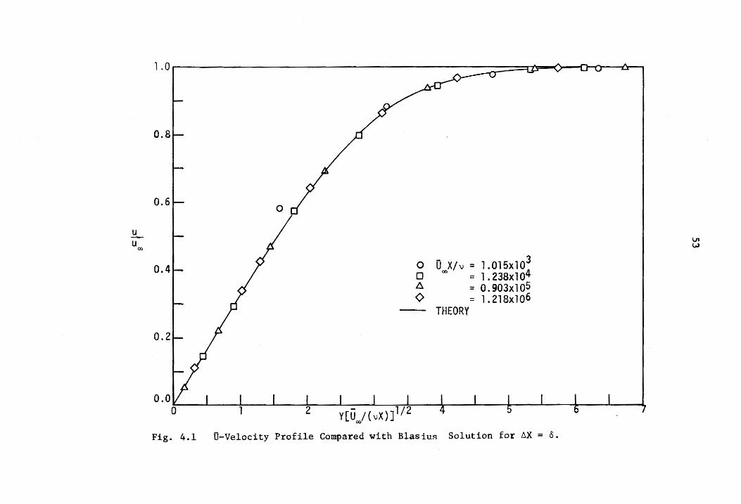
Fig. 4.1 U-Velocity Profile Compared with Blasius Solution for ~x = o.

V(O,~l/v) 1/2

o 00

1.0'

0.8

0.6

0.4

0.2

o o ~

<>

OooX/v : 1.OlSX10! = 1.238xlOS - O.903xl06 = 1.218xlO

-- THEORY

I I I ,

0.00 ~. 2 Y(Uoo

/(vX)1/2 4 6 5

Fig. 4.2 V-Velocity Profile Compared with Blasius Solution for 6X = o.

o

7

\.II .l:"-

u u

00

1.0. __ Q 0 0-,

A 0 X(.; 00

o

0.2 - THEORY

0.0 1 .0 2.0 Y[U,.(/ ('.lX) ] 1/2

= 1.18xl04 , ~X = 8/2 = 1 .81xl04 , ~x = 46

4.0 5.0 6.0

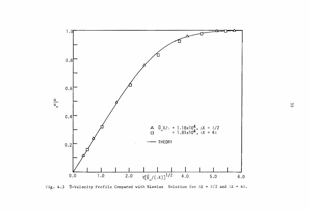
• 4.3 O-Velocity Profile Compared with Blasius Solution for ~x = 6/2 and tX = 46.

V1 V1

1.0-·-------------------------------------------------------------

o o

0.8

0.6

V(Oxxr\.~) 1/2

0 Xl

I v \Jl (j\

0.4

0.2 4 ~ u X/~ = 1.18xlO, = 6/2 o 00 = 1.81xln4, 6X = 48

- THEnRY

0.00 .0 6

Fig. 4.4 V-Velocity Profile Compared with Blasius Solution for 6X 8/2 and ~x 46.

2Tw pO!

.0151~--------------------------------------------------------~

.012

o

Fig. 4.5

U X/v 00

o NUMERICAL - THEORY

Skin-Friction Coefficient Compared with Blasius Solution.

Vl ---J

58

One of the major questions when solving a problem numerically

is: How large a step size can be taken without affecting the results

appreciably? Fig. 4.1 and 4.2 show the U and V profiles for a 6X

step equal to the boundary layer thickness. Obviously at the leading

edge this criterion breaks down because at the leading edge the

boundary-layer thickness is zero. Therefore, at the leading edge 20

steps, equal to 0.001 in., were taken in the X-direction. The step

size was then increased by 10% per step until the step size was equal

to the boundary layer thickness. The boundary layer thickness, 0,

was set at the y-location where u - = u

00

0.99. The total solution,

however was carried out in the y-direction until u u

> 0.99999 and 00

at the next y-location the boundary conditions were imposed. The

choice of the criterion for the solution thickness was somewhat

arbitrary but the following reasoning justified to some extent this

value. Several parametric studies for this flow circumstance showed

that the results were virtually unaffected when the solution was only

taken to u u

00

> 0.9999. However, it was desirable to insure that the

outer region flow in the boundary layer was definitely not affected by

the finite solution thickness. Thus, the higher limit was placed on

the size of the solution thickness with the knowledge that the total

number of grid points in the y-direction increased proportionally.

For the two- and three-dimensional turbulent flows to be inves-

tigated, the near wall region of the boundary layer is of some impor-

tance. To obtain a wall shear stress value from the velocity gradient

59

and the dynamic viscosity, the velocity gradient at the wall should

be determined from the velocity field within the viscous sublayer.

Also of importance, when investigating three-dimensional boundary

layer flows, is the limiting wall streamline direction which again

requires detailed knowledge of the velocity field in the immediate

vicinity of the boundary surfaces. Thus, near the wall five y-grid

locations spaced at .001 in. were used and at each subsequent y-Iocation

~y was increased by 10%. Since the results for the laminar flow

test case were in such good agreement with theory no further study

was made for the y-grid spacing for this case.

Figur~4.3 and 4.4 show the typical dependence that the solution

had on the 6X increment. Since the results for 6X = o 2 were virtually

indistinguishable from those of a step size of 6X = 0, the latter

step size was taken. Note also that for 6X equal to 40, the computer

solution began to show a definite deviation from the exact solution.

In all of these runs the V-profile was not predicted as closely

as was the U profile. This small error was directly attributed to

the finite difference approximation used for the continuity equation,

Eq. 3.29a, for which the truncation error was of order ~x.

Figure 4.5 shows the variation of the skin friction coefficient

with Reynolds number. For laminar flows and turbulent flows the wall

shear stress is proportional to the velocity gradient at the wall.

Thus this figure is a representation of the accuracy of predicted

velocity gradients in the y direction at the wall, and also a check

60

on the method of determining the wall shear stress given below

T W

u u (i, 2. k)

DY (4.1)

Again the good agreement substantiated the validity of the numerical

solution.

B. Turbulent Two-Dimensional Flow

Because of the nature of turbulent flows, exact analytical

solutions of the turbulent boundary-layer equations do not exist for

even the simplest of flow geometries. To verify the validity of

the computer program, experimental data, empirical correlations, and a

simple momentum integral solution were used.

The results of the program were compared to the generally accepted

wall-wake model proposed by Coles [36,39] and are shown in

Fig. 4.6. This figure clearly shows the development of the wake profile

as the velocity profile developed. In the outer regions the wake

function reaches a maximum and for zero pressure gradient flows the

u equilibrium value for the "strength of the wake component" /::,. * - u U

006ll should be approximately 2.7 according to Col~s [36] for v

> 6000. UX

00

The comput~r results shown in Fig. 4.6 for -- - 5.48 x 106 had a U

008ll value of

v of approximately 9,000 and the "strength of the wake

component" was slightly over 2.5. This latter value was within the

scatter of the experimental data from which the average value of 2.7

was obtained.

28-i-------------------------------------------------=~~7~--~~

u u*

C9' ;~ 0000

&. 0 D Cl

0 0

cS£l

~o 20 40

DUX/v = 4.21xl03 o 00 = 6.79xl04 A = 5.48xl06

80 100 400 800 1000 2000 4000 8000 10,000 Yu*/v

Fig. 4.6 Development of Streamwise Turbulent Velocity Profiles Compared with the Law of the Wall.

(J\ ....

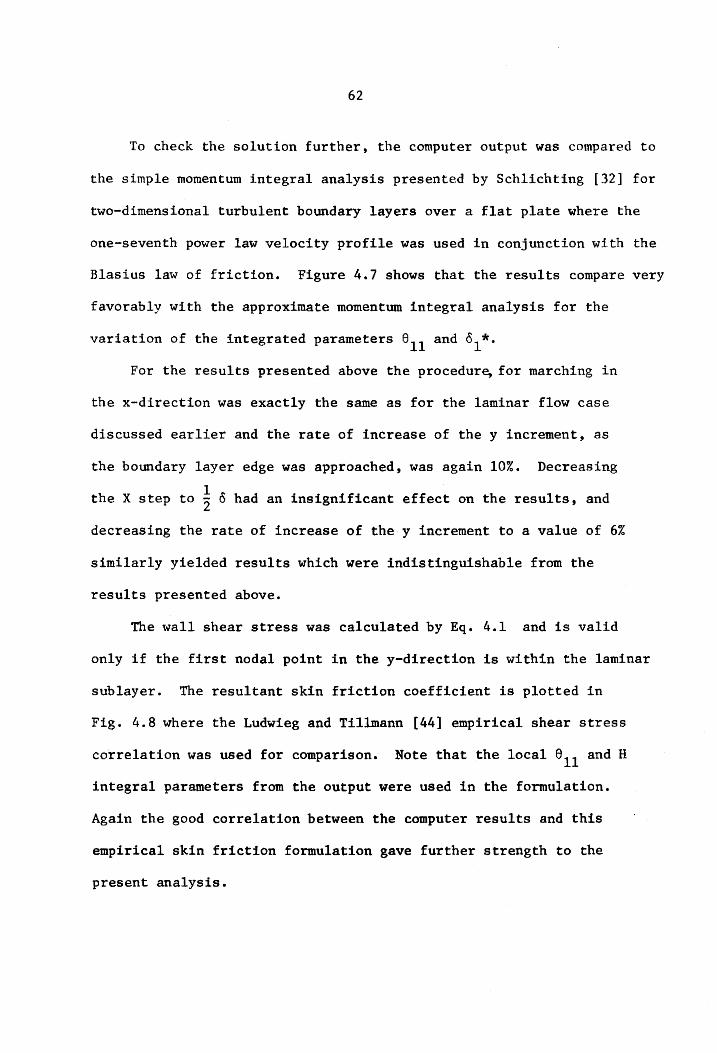
62

To check the solution further, the computer output was compared to

the simple momentum integral analysis presented by Schlichting [32] for

two-dimensional turbulent boundary layers over a flat plate where the

one-seventh power law velocity profile was used in conjunction with the

Blasius law of friction. Figure 4.7 shows that the results compare very

favorably with the approximate momentum integral analysis for the

variation of the integrated parameters 811 and 01*.

For the results presented above the procedur~ for marching in

the x-direction was exactly the same as for the laminar flow case

discussed earlier and the rate of increase of the y increment, as

the boundary layer edge was approached, was again 10%. Decreasing

the X step to ~ 0 had an insignificant effect on the results, and

decreasing the rate of increase of the y increment to a value of 6%

similarly yielded results which were indistinguishable from the

results presented above.

The wall shear stress was calculated by Eq. 4.1 and is valid

only if the first nodal point in the y-direction is within the laminar

sublayer. The resultant skin friction coefficient is plotted in

Fig. 4.8 where the Ludwieg and Til1mann [44] empirical shear stress

correlation was used for comparison. Note that the local ell and H

integral parameters from the output were used in the formulation.

Again the good correlation between the computer results and this

empirical skin friction formulation gave further strength to the

present analysis.

63

O.25~-----------------------------------------------,

0.20

O. 15

4* or 1 811 , in.

o. 10

0.05

6*~ 1 '" 0

o NUMERICAL - THEORY

o

o.oo~ ____ ~~~ _____ ~~ ____ ~~ ____ ~~ ____ ~ lxl0 6 2xl06 3xl0 6 4xl0 6 5xl0 6 6xl0 6

Fig. 4.7 Development of ell and 0t Compared with a

Momentum Integral Analysis.

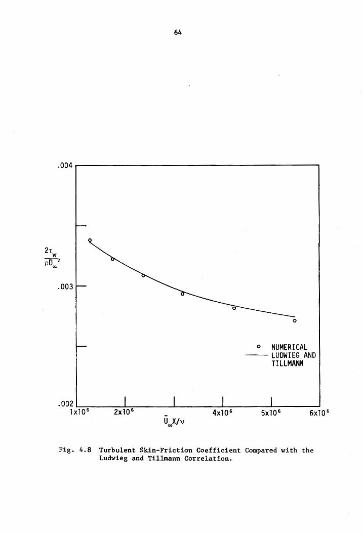
64

.004~-------------------------------------------,

.003

o

o NUMERICAL -- LUDWIEG AND

TIllMANN

.002~~ ____ ~~ ____ ~~ ______ ~ ______ ~ ______ ~ lxl0 6 2xl0 6 - 4xl0 6 5xl0 6

U X/v co

Fig. 4.8 Turbulent Skin-Friction Coefficient Compared with the Ludwieg and Tillmann Correlation.

65

To investigate the solution for adverse pressure gradient flows,

which are probably the most critical test cases, the data obtained

by Schubauer and Klebanoff [45] in a mildly adverse pressure gradient

were used for comparison. The initial profile was obtained from a

best fit law of the wall profile (see Figs. 4.9 and 4.10) using the

data, at the test location at 19 ft from the leading edge, given in

the proceedings of the Stanford Conference [46].

i) U 00

154.1 ft/sec

ii) 0 2.5798 in.

iii) Uoo 30.4 ux

iv) 2t"w _ 0.002164 --2: -on 00

The external velocity field was approximated by Eq. 42 between

x = 19.0 ft and X = 21.S ft.

U = 5.8425 (X _ 17.3)°·44231 00 0.42231 lOX + 326.79 (4.2)

where X is in ft and Uoo

is in ft/sec.

The predicted velocity profiles are shown in Fig. 4.11 and 4.12

for X = 20.5 ft and X = 21.5 ft, respectively.

Initial runs for adverse pressure gradient flows were made in

which the ~x step size was equal to the boundary layer thickness. These

1 I results were compared to those for ~X = 2 0 and ~X = 4 O. The

difference between the latter two runs and the run for ~X = 0 cannot be

shown graphically because of the small deviations between the runs. One

measure of the difference between runs was to note the percentage change

of the velocity at the first nodal location above the boundary surface

u u*

22

14

10 [ 0 10

Yu*/v

o

0 0

0 0

oo:P DO

o o

o o

EXPERIMENTAL DATA APPROXIMATE FIT

Fig. 4.9 Initial Law of the Wall Fit to Schubauer and Kl.e.banoff's Experimental Data at X = 19.0 ft.

0"1 0"1

u u

00

67

1 .0

o.

-- NUMERI CAL o EXPERIMENTAL

0.4

o

Fig. 4.10 Initial V-Velocity Profile for Schubauer and Klebanoff Geometry in Physical Coordinates at X = 19.0 ft.

5

68

at an arbitrary distance downstream. The results, at the location

x = 21.5 ft as the test point, were compared as described above, and

yielded the following information:

Approximate Deviation 6X increment (Compared to 6X = 0/4)

6X = 0 0.9%

~X 1/2 0.08%

6X = 1/4 0%

It was desirable to have an increment in the X direction which

would vary as the pressure gradient varied since for zero pressure

gradient flows the 6X step was equal to o. Thus, the following

parameter was introduced in an effort to modify the nondimensionalized

X increment, x,

u 00

~<-a du 00

(4.3)

where a is an arbitrary constant and ~X was not to exceed the value of O.

For a equal to 0.005, 6X at 19 ft was approximately equal to 0 but at

1 X = 21.5, AX was just under 2 o. The deviation of this run for

~ = ~ 0 was noted in the 4th significant digit. Reducing a to a value

1 of 0.003 yielded essentially the same results obtained for ~ = 4 0 and

a further reduction in the value of a yielded an insignificant change in

the results. Thus the results shown in Figs. 4.11 and 4.12 are for a val-

ue of a = 0.003. The Y increment was 0.002 in. for the first five grid

locations, then successively increased by 10% through the boundary layer.

u Uoo

69

1.0-------------------------O~=-------------,

0.8

0.6

0.4

0.2

NUMERICAL o EXPERIMENTAL

o 1 2 3 4 Y,in.

Fig. 4.11 U-Velocity Profile Compared with Schubauer and Klebanoff's Experimental Data at X = 20.5 ft.

5

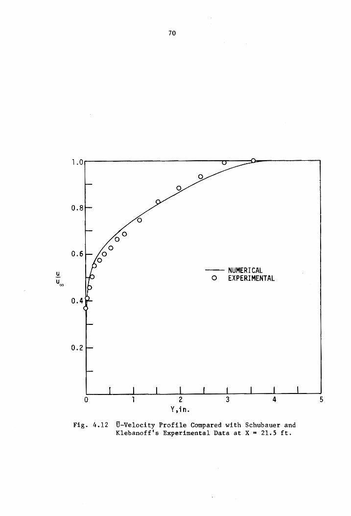
u u

00

70

1.O------------------------------~----~~----------~

0.6

-- NUMERICAL o EXPERIMENTAL

0.4

0.2

o 1 2 3 4 Y ,; n.

Fig. 4.12 U-Velocity Profile Compared with Schubauer and K1ebanoff's Experimental Data at X = 21.5 ft.

5

71

This increase of the Y increment near the wall from 0.001 in. to 0.002

in. was necessary to accommodate the thickness of the boundary layer

under investigation, which was more than twice as thick as those pre-

viously mentioned. The first y location was, however, maintained with-

in the laminar sublayer.

About 40 steps of 0.001 in. in the X direction were taken before the

larger step sizes were imposed. This region allowed the computer

solution to smooth out the input u-velocity profile to conform to the

finite difference equations and allowed for the development of the v

profile.

Finally Cebeci [8] has introduced a correction factor, to compen-

sate for compressibility effect, boundary layer suction and blowing,

and pressure gradients, on the parameter, A, introduced in the

van Driest mixing length hypothesis, Eqs. 3.l7a and 3.l7b.

(4.4)

Since this correction assumes previous knowledge of the wall shear stress,

an iteration procedure was followed at each new location to determine the

proper value of Aeff that was consistent with the shear stress. Using

this correction factor the skin friction coefficient was decreased

approximately 0.1% at X = 21.5 ft when compared to the results pre-

viously described. To generalize this model into three-dimensions

would require the introduction of a non-scalar mixing length because

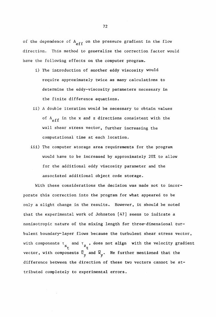
72

of the dependence of Aeff on the pressure gradient in the flow

direction. This method to generalize the correction factor would

have the following effects on the computer program.

i) The introduction of another eddy viscosity would

require approximately twice as many calculations to

determine the eddy-viscosity parameters necessary in

the finite difference equations.

ii) A double iteration would be necessary to obtain values

of Aeff in the x and z directions consistent with the

wall shear stress vector, further increasing the

computational time at each location.

iii) The computer storage area requirements for the program

would have to be increased by approximately 20% to allow

for the additional eddy viscosity parameter and the

associated additional object code storage.

With these considerations the decision was made not to incor-

porate this correction into the program for what appeared to be

only a slight change in the results. However, it should be noted

that the experimental work of Johnston [47] seems to indicate a

nonisotropic nature of the mixing length for three-dimensional tur-

bulent boundary-layer flows because the turbulent shear stress vector,

with components T and T ,does not align with the velocity gradient x t Zt

vector, with components U and W. He further mentioned that the y y

difference between the direction of these two vectors cannot be at-

tributed completely to experimental errors.

73

C. Plane of Symmetry and Three-Dimensional Results

Two three-dimensional solutions were obtained for which experi­

mental data were available. The first solution was for the Johnston [28]

data and the second was for the experimental data presented by Hornung

and Joubert [29].

Figure 4.13 shows the match to the profile at station D-8 in the

Johnston experiment. To obtain this match a two-dimensional boundary

layer was developed from a leading edge of a flat plate some 62 in.

before the match point with the external velocity equal to the velocity

at the match point. The fit was a compromise between the following

criteria:

i) Matching the integrated parameters 611 and o! as closely

as possible,

ii) Matching the actual velocity profile, and

iii) Developing a profile over the approximate actual lead-in

section length.

To generate an accurate solution, the free-stream flow field should

approximate as closely as possible the actual flow condition encountered

in the experiment. Figure 4.14 shows the experimentally measured field

and the external velocity field as predicted from the potential flow

solution for this geometry. Due to the slight acceleration of the

fluid caused by boundary layer growth on the floor and the ceiling of

the test section, the predicted external velocity noticeably deviated

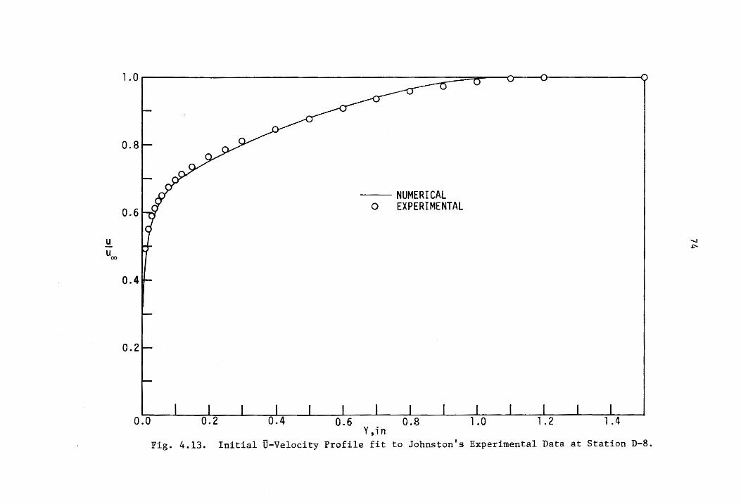
U

Uoo

1.0 I _;( 0 0 0

-- NUMERI CAL o EXPERIMENTAL

0.0 0.8 Y.in

Fig. 4.13. Initial U-Velocity Profile fit to Johnston's Experimental Data at Station D-S.

...... ~

u2. 00

l.°tF========~d~==~~---------------------------------------'

0.9

--THEORY o EXPERIMENTAL DATA

0.5, \ I

o 4 8 12 16 20 24 28 X,in

Fig. 4.14 External Velocity Field on the Plane of Symmetry for the Johnston Geometry.

....... V'I

76

from the actual velocity as the end wall was approached (especially

after a distance of about 24 in. from station D-8). This deviation

resulted in a larger adverse pressure gradient than actually

experienced experimentally by Johnston. Thus, the information obtained

from the computer solution should exhibit characteristics which are

attributable to this larger adverse and therefore a larger transverse

pressure gradient when compared to the experimental data.

This problem directly affected the location of the

separation point along the plane of symmetry. The experimental results

from observing the flow while smoke was injected into the stream and

also using a wall streak test qualitatively showed the separation point

on the plane of symmetry to be about 31 in. from station D-8. The

computer results showed separation to occur at about 27.7 in. downr

stream of the match point or about 3.3 in. before the experimentally

determined point. East [27] numerically showed separation to occur

at approximately 28 in. The reason for the difference between these

two numerical solutions was not precisely determined~ but it is noted

that the nature of the finite diffe~ence approximations are dissimilar

to the extent that one of the truncation error terms in the Dufort-

Frankel finite difference approximations is For flows near

separation u becomes large and the solution is directly affected by xx

this truncation error which possibly accounts for the discrepancy

noted above. For the present numerical technique the corresponding

truncation error term for the momentum equation was u (6x)2, a much xxx

smaller term.

77

Figures 4.lSa through 4.1Sd show typical predicted u-velocity

profiles along the plane of symmetry. For all of these cases the

velocity near the wall was underpredicted. This was partially

caused by the initial fit at station D-8 which also exhibits this same

characteristic due to the necessary compromise to obtain the match

point profile.

For the plane of symmetry solution, the quantity wz was

calculated from Eq. 3.24b. However, only an approximate comparison

with experimental evidence was possible because of the large z

spacing between data locations. Figure 4.16 shows the results at

the location 26 in. from the match point. The wz derivative was approx­

imated by taking a simple difference using the data nearest the plane of

symmetry. Also shown on this figure are the results presented by

Mellor [21] and East [27). The numerical wz profile seemed to

overpredict the experimental data. This is expected since wz

reaches a maximum on the plane of symmetry and the derivative

formed from the experimental data was obtained by using the w

velocities at Z = + 2.5 in., therefore predicting lower values

than actually expected. Further downstrea~ comparison was impossible

since the present program predicted separation before the next

experimental location. East was able to compare with Mellor's

results at both 28 in. and 30 in. because they both fit a polynomial

expression to the experimental velocity field on the plane of

symmetry. However, when the present solution at 27.7 in. is

compared to their results at 28 in. and the experimental results

U Uoo

1.0r 0 0 (( ~i)

0.8

0.6

0.2

0.0

o

0.6 y' 0.8 ,1 n

0.2 0.4

NUMERICAL EXPERIMENTAL

1.0 1 .2 1.4

Fig. 4.1Sa V-Velocity Profile Compared with Johnston's EXperimental Data at Station D-6.

-..J 00

u u

00

1 .0

0.8

NUMERICAL o EXPERIMENTAL

0.2

0.0 0.2 0.4 0.6 Y,in 0.8 1 .0 1 .2 1 .4

Fig. 4.lSb U-Velocity Profile Compared with Johnston's Experimental Data at Station D-XB.

""-J \!)

U

Uoo

1 .0 I ~----------------------~~~~rf--~

0.8

0.6

0.4

0.2

0.0 0.2 0.4

o

0.6 0.8 Y,in

NUMERICAL EXPERIMENTAL

1 .0 1 .2 1 .4

Fig. 4.15c U-Velocity Profile Compared with Johnston's Experimental Data at Station D-4.

co o

u u

00

1 .0 I --------------------------------------------------------~~~~==~~o

0.8

0.6

--- NUMERI CAL o EXPERIMENTAL

0.4

0.2

0.0 0.2 0.4 0.6 0.8 1 .0 1 .2 Y,in

Fig. 4.lSd U-Velocity Profile Compared with Johnston's Experimental Data at Station D-X6.

00 f--'

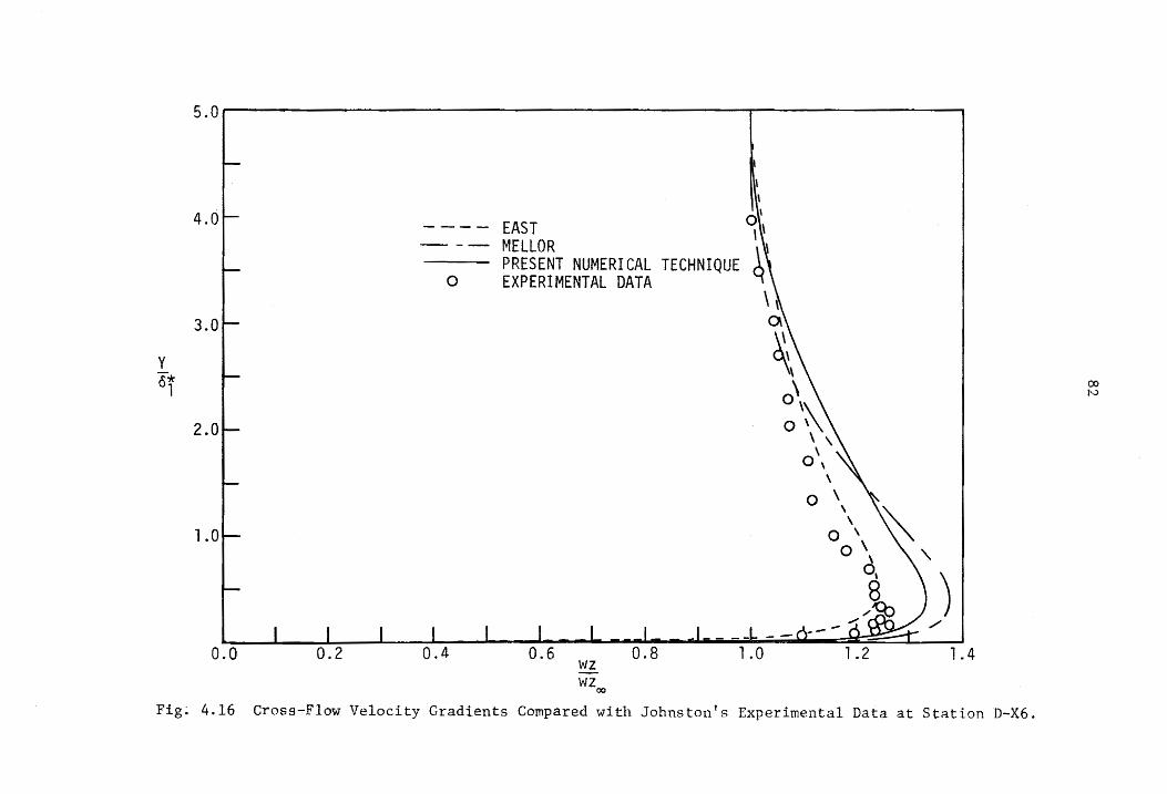
y 6* 1

5.0f~--------------------------------------------------------------------------

4.0 - --- EAST - -- MELLOR

PRESENT NUMERICAL TECHNIQUE o EXPERIMENTAL DATA

3.0

) /

0.0 1 .4

WZoo

Fig. 4.16 Cross-Flow Velocity Gradients Compared with Johnston's Experimental Data at Station D-X6.

ex> N

83

at 28 in., the present analysis yielded a result similar to the

results shown in Fig. 4.16.

Figure 4.17 shows the variation of the momentum thickness

along the plane of symmetry. The numerical solution predicted this

growth very well up to about 26 in •• where the momentum thickness

began to increase more rapidly than the experimental results. This

is due to the discrepancy between the actual and theoretical

free-stream velocity fields, especially in velocity gradients. A

similar result is shown in Fig. 4.18 for the development of o~

along the plane of symmetry.

Figures 4.19 and 4.20 show the velocity profiles obtained

off the plane of symmetry. The results are shown in streamline

coordinates because this is generally the format in which experi-

mental profiles are presented in the literature. The U -velocity s

profiles were generally in good agreement with the experimental

profiles. TheW component of velocity was consistently slightly s

larger than that of the experimental profiles. This same effect was

experienced by East and the probable cause was the larger cross-

flow pressure gradient obtained from the potential flow solution,

as discussed earlier.

Many experimentalists (Francis and Pierce [48], Klinksiek and

Pierce [49], Gardow [50J, Johnston [28], Hornung and Joubert [29],

Smith [51], Smith [52], Lewkowicz [53]) have recorded data which

seem to imply the existence of a collateral layer in the near wall

region of three-dimensional turbulent boundary-layer flows. However,

O.4~i----------------------------------------------------------------------~

NUMERICAL o EXPERIMENTAL

'11 tin

o

o. 1

o.o~, __ ~ ____ ~ __ ~ __ ~~ __ ~ __ ~ __ ~~ __ ~ __ ~ __ ~~ __ ~ __ ~ ____ ~ __ ~ __ __ o 4 10 24 16 20 8 28

X,in

Fig. 4.17 Development of 811

on the Plane of Symmetry Compared with Johnston's Experimental Data.

()) ~

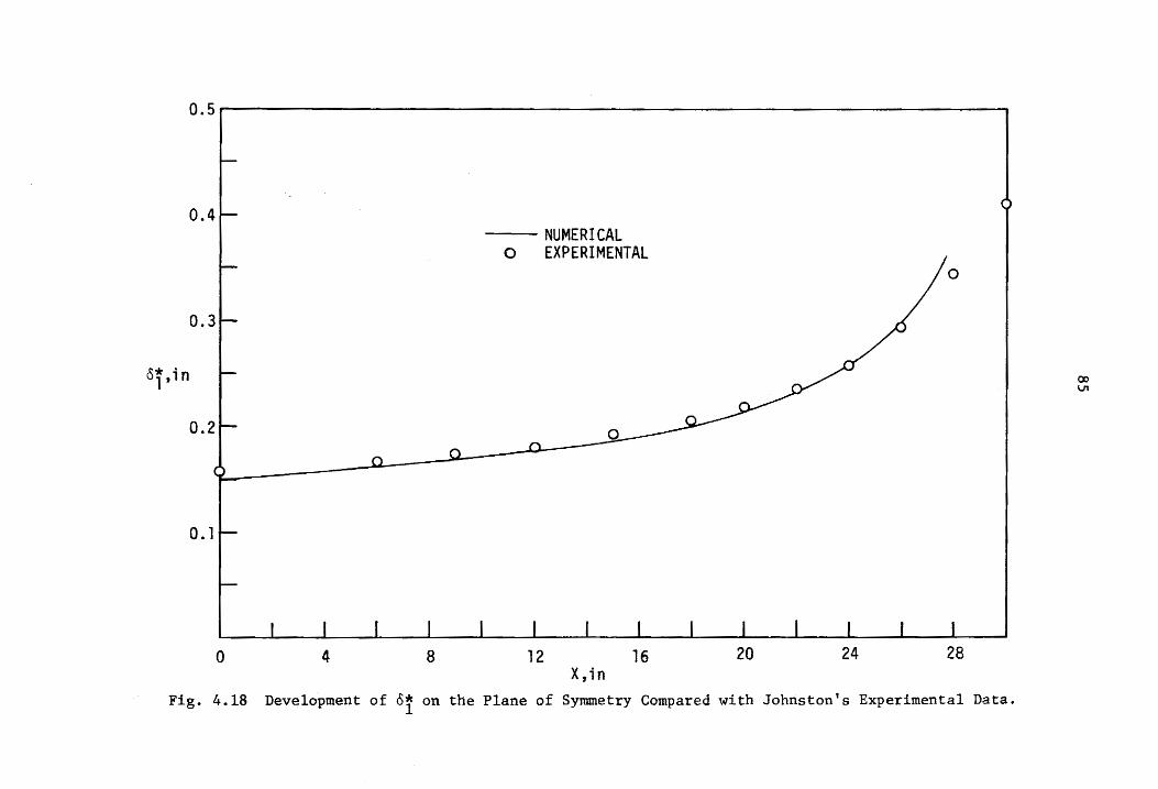
0.5i~----------------------------------------------------------------------~

-- NUMERICAL o EXPERIMENTAL

o

o

o l'* . 1.)1 ,1 n o

o o

o o

o 4 8 12 16 20 24 28 X,in

Fig. 4.18 Development of o! on the Plane of Symmetry Compared with Johnston's Experimental Data.

(X) ~

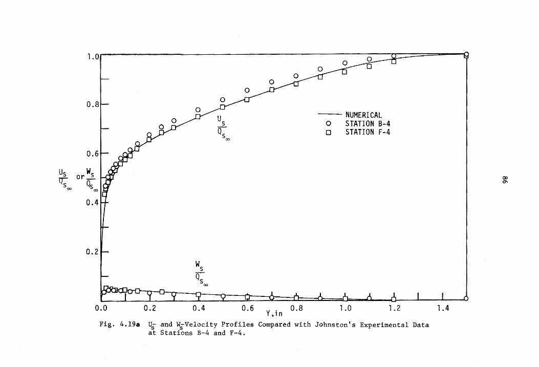
1.0' cc:: 9

0.6

W Us or 2-~ Qs 00 00

0.4

0.2

Ws Qs

00

-- NUMERICAL o STATION B-4 o STATION F-4

0.0 0.2 0.4 0.6 y. 0.8 1 .0 1 .2 ,1 n

Fig. 4.198 Us and WsVelocity Profiles Compared with Johnston's Experimental Data at Stations B-4 and F-4.

1 .4

('X) 0'\

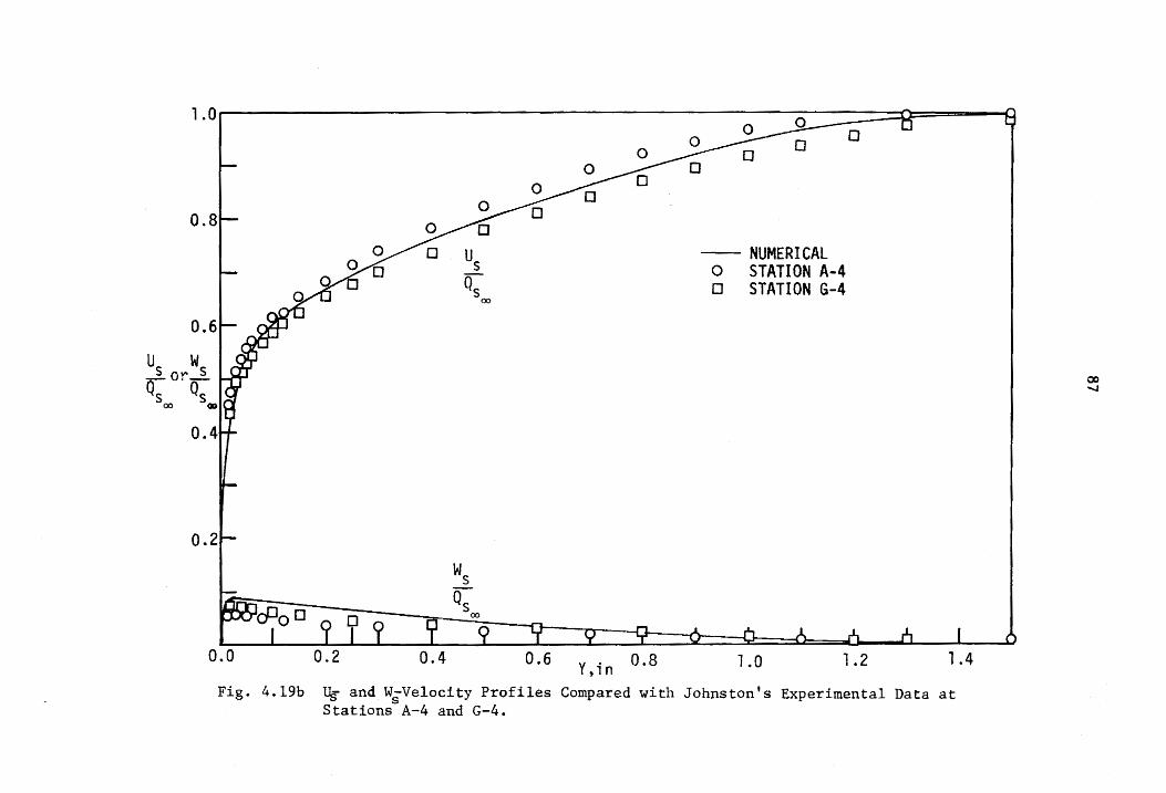
1.0, t"\ -Q= 8

Us Ws -or_ Qs Os

00 CD

0.0 0.2 0.4

Us Os

00

-- NUMERICAL o STATION A-4 o STATION G-4

0.6 y' 0.8 ,1 n 1.0 1 .2 1 .4

Fig. 4.l9b ~ andWsVelocity Profiles Compared with Johnston's Experimental Data at Stations A-4 and G-4.

00 ......

1 . 0 r n::::::::R= e

Us Ws -or­Qs Qs

00 00

Us Qs

00 -- NUMERICAL o STATION 8-X6 o STATION F-X6

0.0 0.2 0.4 0.6 Y,in 0.8

Fig. 4.20a Us and WgVelocity Profiles Compared with Johnston's Experimental Data at Stations B-X6 and F-X6.

00 00

1.0 I r\ :J;t 9

0.8

------ NUMERICAL o STATION A-X6 o STATION G-X6

Ws

~ 00

0.0 0.2 0.4 0.6 Y,in 0.8 1.0

Fig. 4.20b ~- and ~Velocity Profiles Compared with Johnston's Experimental Data at Stations A-X6 and G-X6.

(),) \,()

90

the results of the present investigation indicated that the local

streamline direction monotonically increased as the wall was

approached as exhibited in Figs. 4.21 and 4.22 for two typical

locations. This behavior was also detected by East. As shown

in Fig. 4.23 a significant variation of the flow angle occurs in

a very small region close to the wall and generally much closer to

the wall than is accessible to ordinary experimental techniques.

Rogers and Head [54] developed a probe that was especially designed

for minimum interference with the fluid and they showed experimentally

that the flow angle had a monotonically increasing characteristic

in the near wall region.

The momentum thicknesses and the displacement thicknesses,

with respect to a local streamline coordinate direction, are shown

in Figs. 4.24 through 4.26. Again the predicted results were

within the range of the experimental data presented by Johnston.

These figures also illustrate the asymmetry of the flow with respect

to the z = 0 plane.

Several parametric studies were undertaken to observe the

dependency of the solution on the size of ~x, ~y, 6z. The ~x

step was governed by Eq. 4.3 where a was taken as the previously

determined value of 0.003. Decreasing this value had negligible

effect on the results. Increasing this value had negligible effect

on the u-profile, but influenced the v-profile and tended to

stave off the predicted separation point to a location further

downstream. For example, with a - 0.005 the point of separation

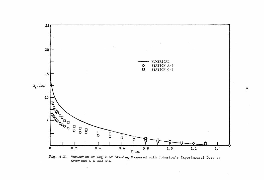
(l ,deg s

25~1 -----------------~

20

I 15

1\ 10

5

0

Fig. 4.21

o o

0.2 0.4 0.6 Y,in.

NUMERICAL 0 STATION A-4 0 STATION G-4

0.8 1.0 1.2

Variation of Angle of Skewing Compared with Johnston's Experimental Data at Stations A-4 and G-4.

\0 .....

25~1------------------------------------------------------------------------~

as ,deg NUMERICAL

o STATION 8-X6 o STATION F-X6

o 0.2 Y,in.

Fig. 4.22 Variation of Angle of Skewing Compared with Johnston's Experimental Data at Stations B-X6 and F-X6.

\Q .....,

as • deg

93

25~------------------------------------------~

¢ NUMERICAL 20 o STATION B-X6

o STATION F-X6

15

<> <> <> <> <> <> <> <> 10 0

0

0

0

5

O~ __ ~ __ -L __ ~ ____ ~ __ ~ __ ~ __ ~ ____ ~ __ ~ __ ~

o .005 .010 .015 .020 Y. in.

Fig. 4.23 Variation of Angle of Skewing in the Near Wall Region Compared with Johnston's Experimental Data at Stations B-X6 and F-X6.

.025

3.01 ------------------------------------------1

ell,in.

EXPERIMENTAL DATA V I = -5.0 in. A = +5.0 in. o = -2.5 in. <> = 2.5 in.

NUMERICAL

Z :: o V

v

<>

v

O.l~, __ ~ __ ~--L-~~-L--~--J---L---L-~---L---L--~--L-~ a 4 16 28 8 20 12 24

X,in.

Fig. 4.24 Development of 811

off the Plane of Synmetry Compared with Johnston's Experimental Data.

\0 +'-

0.5~1-----------------------------------------------------------------------

0.4

I " ll. 0 <>

EXPERIMENTAL DATA Z = -5.0 in.

= 5.0 in. = -2.5 in. = 2.5 in.

0.3 - NUMERICAL

8* . 1 ,1 n

0.2

0.1

v Z = :!:

Z =

o 4 8 12 x ~ in.

16

Fig. 4.25 Development of 8t off the Plane of Symme.try Compared with Johnston's

Experimental Data.

<> 6 o

v

\0 \J1

.05 I J

.04

. 03

813 , in.

.02

.01

o 4

\l /::,.

o <>

8

EXPERIMENTAL DATA Z = -5.0 in.

= 5.0 in. = -2.5 in . = 2.5 in.

NUMERICAL

X,; n.

Z = ± 5 .. 0 o

20

Fig. 4.26 Development of 613 off the Plane of Symmetry Compared with Johnston's Experimental Data.

o

\0 C1'

97

was located approximately 0.02 in. further downstream and the

V-velocity component at the free stream exhibited about a 25%

decrease at a distance of 26 in. from the match point.

Instead of a successive increase of ~y of 10% through the

boundary layer from an initial ~Y of 0.001 in., a rate of increase of

6% was used. The differences between these two rates of increase

were insignificant for the v-profile, but the u and w velocities

near the wall changed by as much as 0.5% as separation was approached.

Halving the step size of ~z from 0.75 in. to 0.375 in. resulted

in a small change (third significant digit changed by about one unit)

and thus did not merit the increase of computer time.

To summarize, the values of the increments used were:

i) l:::.x -1

= 0.003 tJoo(dUoo) dx

ii) l:::.Y = 0.001 in_until Y = 0.005 in.; then

l:::.Y was successively increased by 6%

iii) l:::.Z = 0.75 in.

The total run time for this solution including a 62 in. two-dimensional

lead-in section was approximately 16 min and 30 sec on an IBM 360-65.

This time does not include the 32 sec necessary for compiling when

the object deck is unavailable.

To further substantiate the results of this program for three-

dimensional turbulent boundary-layer flows, the Hornung and Joubert

{29] geometry was investigated.

To match the profile at station 10, a two-dimensional turbulent

boundary layer was developed from a distance of 22 ft from the

98

center of the cylinder to 4 ft from the center of the cylinder at

which point the three-dimensional solution was initiated. The

actual centerline of the cylinder was 17 ft down stream of the

leading edge which was some 5 ft shorter than the necessary length

to generate an adequate fit at station 10. The reason for this

additional length was the presence of a slightly divergent inlet

channel, which possibly imposed a small adverse pressure gradient,

and resulted in an increased rate of boundary layer growth in this

test section. The final match, shown in Fig. 4.27, was the result

of several trial runs in which the inlet length was varied to

allow the computed boundary layer thickness at station 10 to be

approximately the same as the experimental value.

Figures 14.28 and 14.29 show the results of the Hornung and

Joubert geometry at stations 12 (Z = 6 in.) and station 14 (Z = 12 in.),

respectively. The results were in even better agreement with

experiment than previously experienced in the Johnston geometry.

The probable reason for this better agreement was the lesser

influence of the confining boundaries. In the Hornung and Joubert

geometry the test section dimensions were large compared to boundary

layer thicknesses on the walls, the latter having a negligible

influence on the potential flow in the center portions of the

channel. For Johnston's apparatus the distance between the top

and bottom surfaces was 8 in. and the boundary layer thickness

was of order 1.5 in., and this close spacing caused the experimental

velocities to deviate from the theoretical values due to the

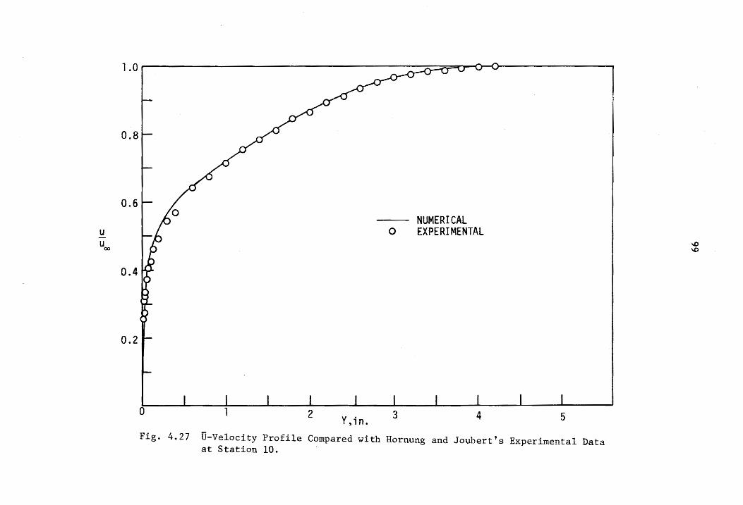
U Uoo

1 .0 I _---rr--n-v--0--<

0.8

0.6

o

Fig. 4.27

o

Y tin.

NUMERICAL EXPERIMENTAL

U-Velocity Profile Compared with Hornung and Joubert's Experimental Data at Station 10.

I,C)

\0

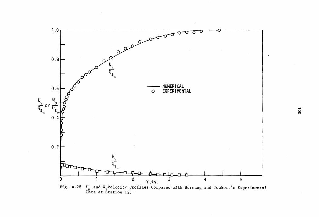
1 0 _, A II • I 0\---------.,

0.8

0.6

u W .2.. or .2. Qs Qs

00 00

0.4

0.2

o Fig. 4.28

1

Ws Qs

00

2

-- NUMERICAL o EXPERIMENTAL

Y,in. 3 4 5

Us and WsVe10city Profiles Compared with Hornung and Joubert's Experimental Data at Station 12.

t--I o o

1.0. _ 0 0 Ol------

0.8

0.6

U w i or 2.. Qs Os

00 00

Ws Qs

00

NUMERICAL o EXPERIMENTAL

a 1 2 Ytin. 3 4 5

Fig. 4.29 Us and WsVelocity Profiles Compared with Hornung and Joubert's Experimental Data at Station 14.

..... o .....

102

displacement effects of the boundary layers.

The solution was continued until the separation point was reached.

Hornung and Joubert did not state explicitly at what position separation

occurred. However, they did show a profile at station 9 for which

back flow was not noted. The present program predicted separation on the

plane of symmetry to occur at 2 in. before this experimental station.

Again separation was determined by the boundary layer velocity near the

surface being equal to or less than zero.

A parametric study was made to determine the step sizes necessary

to insure their negligible influence on the results. Again, the x step

size was governed by Eq. 4.3 with cr = 0.003 with insignificant change for

smaller values of cr. Because of the greater thickness of the boundary

layer for this geometry the Y increment near the wall was 0.002 in. for

five locations and subsequently was increased by 6% as determined by the

Johnston geometry. The value for 6Z was 1.5 in. and a reduction of this

value to 1 in. affected the U and W profiles by less than 0.05% at

location 12.

The total computer time required for the solution for the Hornung

and Joubert geometry was about 13 min. This time also included the

18 ft distance required to develop the two-dimensional boundary-layer

in the lead-in sections. Agai~ compiling time is not given since for

production runs an object deck would be used to obviate the necessity

of repeated compilations of the program.

103

Since the shear stress profiles were not measured in either

the Johnston or the Hornung and Joubert experiments, direct

comparison with measured data was impossible. However, the shape

of these profiles are of general interest in three-dimensional

flows since they were determined from a scalar mixing length

hypothesis. Figures 4.30 and 4.31 show typical shear stress profiles

in both the X and Z directions, respectively.

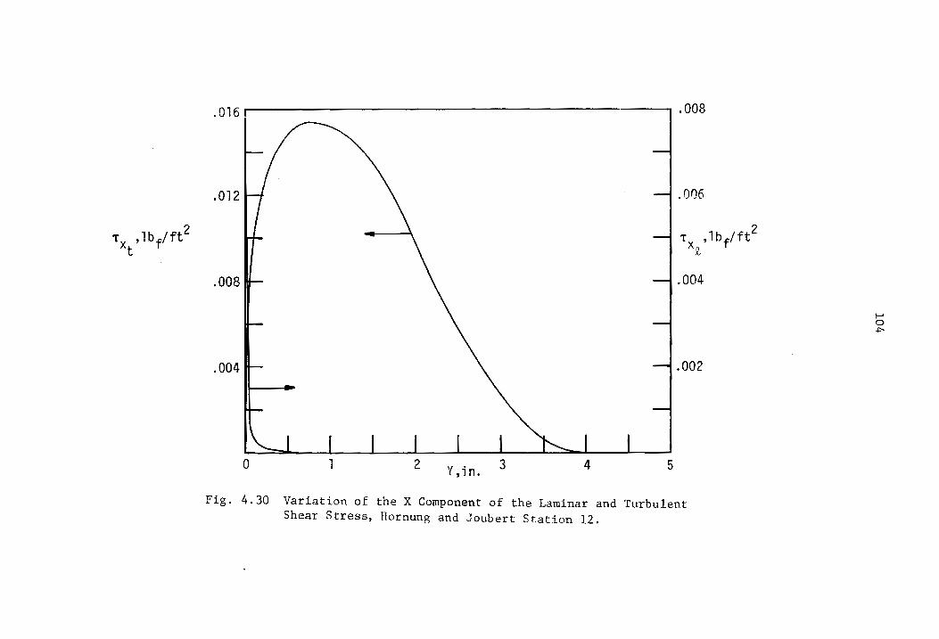
2 Tx ,1b f /ft t

.0161~~ -------------------------------------------- .008

.012 H \ --1 .006

H- --\ -1 TXt' 1 bf /ft2

.ooar \ 1.004

.002

o 1 2 y ,i n. 3 5

Fig. 4.30 Variation of the X Component of the Laminar and Turbulent Shear Stress, Hornung and Joubert Station 12.

....... 0 ~

.0012

.0008

lOS

.0024

.0016

.0008

N -4J 4-

PL--~-----+----~----+-----r---~-----t~--1-----t---~ ~

1 2 Y ,i n. 4

..0 ,..... ..

-.0008

-.0016

-.0024

Fig. 4.31 Variation of the Z Component of the Laminar and Turbulent Shear Stress, Hornung and Joubert Station 12.

V. S~ruARY AND CONCLUSIONS

A technique is presented to solve the equations of motion

for a broad class of both two-dimensional and three-dimensional

turbulent boundary-layer flows. An extension of the implicit

numerical finite difference technique, presented by Crank and

Nicholson [37] for unsteady heat conduction, to the three-dimen­

sional equations of motion was introduced to cast the partial

differential equations in a finite difference form.

The method assumed that an eddy viscosity model expressed

in terms of a mixing length was known and the program was

sufficiently generalized to allow the adaptation and subsequent

introduction of other experimental correlations as they become

available. The mixing length model chosen for this investigation

is given by Pletcher [11]. The model was generalized to three­

dimensional flows as given by Prandtl (see Goldstein [34]) and

the mixing length was treated as a scalar function.

The final finite-difference equations were cast into a form

such that the corresponding matrix of coefficients to be solved

were in a tridiagonal form and were easily solved using the

Thomas algorithm [31].

This numerical technique was applied to two-dimensional laminar

and turbulent boundary-layer flows and three-dimensional turbulent

boundary-layer flows from which the following observations and

conclusions were obtained:

106

107

1. The Crank-Nicholson finite-difference scheme for writing

finite-difference equations yielded a stable and convergent

method for all the cases tested.

2. The Blasius profile for laminar two-dimensional zero

pressure gradient flows was predicted and good agreement

with the theoretical profile was obtained.

3. The form of the continuity equation was critical when the

V - velocity profile was unknown as an initial condition.

4. The mixing length hypothesis model yielded good results for

two-dimensional turbulent flows in both zero and adverse

external pressure gradient flows. For three-dimensional

turbulent boundary-layer flows the results were in good

agreement when compared to experimental data.

5. The computational time required for the Johnston [28]

and the Hornung and Joubert [29] geometries was at least

five times faster than the explicit Dufort-Frankel

finite difference technique presented by East [27],

for the same flow circumstances.

6. The concept of a collateral near-wall layer for a three­

dimensional turbulent boundary layer was not substantiated

by the present analysis.

108

7. More experimental turbulence data in three-dimensional

turbulent boundary layer flow circumstances are required

to further validate and improve the turbulent-shear

stress model.

VI. BIBLIOGRAPHY

1. Spalding, D. B., "Theories of the Turbulent Boundary Layer," Applied Mechanics Reviews, Vol. 20, No.8, August 1967.

2. Pierce, F. J., and D. H. Krommenhoek, "Wall Shear Stress Diagnostics in Three-Dimensional Turbulent Boundary Layers," Interim Technical Report No.2, USARO-D Project No. 6858E, September, 1968, (AD 680 973).

3. Thompson, B. G. J., irA Critical Review of Existing Methods of Calculating the Turbulent Boundary Layer,1f ARC R&M 3447, Ministry of Supply, Great Britain, 1964.

4. Hinze, J. 0., Turbulence, Chapter 1, McGraw-Hill Book Company, Inc., New York, 1959.

5. Prandtl, L., "fiber die ausgebildete Turbulenz," a lecture delivered at Zurich in September, 1926, before the International Congress for Applied Mechanics, (translated as nTurbulent Flow"), NACA TN 435, 1927.

6. Townsend, A. A., "Equilibrium Layers and Wall Turbulence," Journal of Fluid Mechanics, Vol. lIt pp. 97-120, August 1961.

7. van Driest, E. R., "On Turbulent Flow Near a Wall,rr Journal of the Aeronautical Sciences, pp. 1007-1011, November 1956.

8. Cebeci, T., "Calculation of Compressible Turbulent Boundary Layers with Heat and Mass Transfer," AIM Paper NO. 70-741 presented at the AlAA 3rd Fluid and Plasma Dynamics Conference, June 1970.

9. Mellor, G. L., "The Effects of Pressure Gradients on Turbulent Flow Near a Smooth Wall," Journal of Fluid Mechanics, Vol. 24, part 2, pp. 255-274, 1966.

10. Mellor, G. L., and D. M. Gibson, "Equilibrium Turbulent Boundary Layers," Journal of Fluid Mechanics, Vol. 24, part 2, pp. 225-253, 1966.

11. Pletcher, R. H., "On a Finite-Difference Solution for the Constant-Property Turbulent Boundary Layer," AIAA Journal, Vol. 7, No.2, pp. 305-311, 1969.

12. ~1aise, G., and H. McDonald, "Mixing Length and Kinematic Eddy Viscosity in a Compressible Boundary Layer," AIM Journal, Volume 6, No.1, pp. 73-80, 1968.

109

110

13. Bradshaw, P., D. H. Ferris, and N. P. Atwell, "Calculation of Boundary-Layer Development Using the Turbulent Energy Equation," ...TournaI of Fluid Nechanics, Vol. 28, part 3, pp. 593-616, 1967.

14. Bradshaw, P., "Calculation of Boundary-Layer Development Using the Turbulent Energy Equation, VII: Three-Dimensional Flow," National Physical Laboratory, AERO Report 1286, 1969.

15. Nash, J. F., "The Calculation of Three-Dimensional Turbulent Boundary Layers in Incompressible Flow,u Journal of Fluid Mechanics, Vol. 37, part 4, pp. 625-642, 1969.

16. Donaldson, C. duP., and H. Rosenbaum, "Calculation of Turbulent Shear Flows Through Closure of the Reynolds Equations by Invariant Modeling," Compilation of Papers Presented at Symposium on Compressible Turbulent Boundary Layers, Sponsored by Langley Research Center, pp. 10.1-10.23, December 1968.

17. Smith, A. M. 0., and T. Cebeci, "Numerical Solution of the Turbulent Boundary-Layer Equations," McDonnell Douglas, Report No. DAC 33735, May 1967.

18. Hartree, D. R., and J. R. Womersley, "A Method for the Numerical or Mechanical Solution of Certain Types of Partial Differential Equations," Proc. Roy. Soc. (London), p. 353, 1937.

19. Smith, A. M. 0., and D. W. Clutter, "Machine Calculation of Compressible Laminar Boundary Layers," AIM Journal, Vol. 3, No.4, pp. 639-647, 1965.

20. Smith, A. M. 0., N. A. Jaffe, and R. C. Lind, "Study of a General Method of Solution of the Incompressible Turbulent Boundary Layer Equations," Douglas Aircraft Division, Report No. LB-52949, November 1965.

21. Mellor, G. L., "Incompressible, Turbulent Boundary Layers with Arbitrary Pressure Gradients and Divergent or Convergent Cross Flows,fI AIM Journal, Vol. 5, No.9, pp. 1570-1579, 1967.

22. Der, J., and G. S. Raetz, "Solution of General Three-Dimensional Laminar Boundary-Layer Problems by an Exact Numerical Method," lAS Paper No. 62-70, January 1962.

23. Dwyer, H. A., "Solution of a Three-Dimensional Boundary-Layer Flow with Separation," AIAA Journal, Vol. 6, No.7, pp. 1336-1342, 1968.

24. Sowerby, L., "The Three-Dimensional Laminar Boundary Layer on a Flat Plate," Journal of Fluid Mechanics, Vol. 22, part 3, pp. 587-598, 1965.

III

25. Flugge-Lotz. I., and F. G. Blottner, Technical Report Number 131, 1962, Division of Engineering Mechanics, _ Stanford University, California. See also Applied Mechanics Reviews, Vol. 15, 1962.

26. Fussell, D. D., "The Study of Numerical Methods for Solving the Laminar Boundary Layer Equations," Doctoral Dissertation, Rice University, Houston, Texas, 1965.

27. East, J: L., "An Exact Numerical Solution of the Three­Dimensional Incompressible Turbulent Boundary Layer Equations,tI Doctoral Dissertation, Virginia Polytechnic Institute and State University, Blacksburg, Virginia, 1970.

28. Johnston, J. P., "Three-Dimensional Turbulent Boundary Layer," MIT Gas Turbine Lab. Report No. 39, 1957.

29. Hornung, H. G., and P. N. Joubert, "The Mean Velocity Profile in Three-Dimensional Turbulent Boundary Layers," Journal of Fluid Mechanics, Vol. 15, part 3, pp. 368-384, 1962.

30. Hunt, J. L., D. M. Bushnell', and I. E. Beckwith, "Finite­Difference Analysis of the Compressible Turbulent Boundary Layer on a Blunt Swept Slab with Leading-Edge Blowing," Analytical Methods in Aircraft Aerodynamics, NASA SP-228, pp. 417-472, Oct. 1969.

31. Ames, W. F., Numerical Methods for Partial Differential Equations, Barnes and Noble, Inc., New York, 1969.

32. Schlichting, H., Boundary Layer Theory, Chapters 7, 18 and 19, Fourth Edition, McGraw-Hill Book Company, Inc., New York, 1960.

33. Frederick, D., and T. S. Chang, Continuum Mechanics, chapter 3, Allyn and Bacon, Inc., Boston, 1965.

34. Goldstein, S., Modern Developments in Fluid Dynamics, Vol. 1, Dover Publications, Inc., pp. 205-210, 1965.

35. Laufer, J., "The Structure of Turbulence in Fully Develope4 Pipe Flow," NACA TN 2954, June 1953.

36. Coles, D., "The Turbulent Boundary Layer in a Compressible Fluid," RAND Corp. Report No. R-403-PR, September 1962.

37. Crank, J., and P. Nicholson, "A Practical Method for Numerical Evaluation of Solutions of Partial Differential Equations of the Heat Conduction Type," Proc. Cambridge Philos. Soc., Vol. 43, pp. 50-67, 1947.

112

38. ~vu, J. C., "The Solution of Laminar Boundary-Layer Equations by the Finite Difference Method," Douglas Aircraft Company, Inc., Report No. SH-37484, June 1960.

39. Coles, D., "The Law of the Wake in the Turbulent Boundary Layer," Journal of Fluid Mechanics, Vol. I, Part 2, pp. 191-226, 1956.

40. Milne-Thompson, L. M., Theoretical Hydrodynamics, The MacMillan Company, New York, 1960.

41. Pai, Shih-I, Fluid Dynamics of Jets, D. Van Nostrand Company, Inc., New York, pp. 9-13, 1954.

42. Traub, J. F., "The Solution of Transcendental Equations," Mathematical Methods for Digital Computers, John Wiley and Sons, Inc., New York, Vol. 2, pp. 171-184, 1967.

43. Richtmyer, R. D., and K. W. Morton, Difference Methods for Initial-Value Problems, Interscience Publishers, New York, second ed., 1967.

44. Ludwieg, H., and H. Tillmann, "Inves tigations of the Wall Shearing Stress in Turbulent Boundary Layers," NACA TM 1285, 1950.

45. Schubauer, G. B., and P. S. Klebanoff, "Investigation of Separation of the Turbulent Boundary Layer," NACA TM 2133.

46. Coles, D. E., and E. A. Hirst, Proceedings: Computation of Turbulent Boundary Layers - 1968 AFOSR - IFP - Stanford Conference, Stanford University, 1969.

47. Johnston, J. P., "Measurements in a Three-Dimensional Turbulent Boundary Layer Induced by a Swept, Forward-Facing Step," Journal of Fluid 1lechanics, Vol. 42, part 4, pp. 823-844, 1970.

48. Francis, G. P., and F .. J. Pierce, "An Experimental Study of Skewed Turbulent Boundary Layers in Low Speed Flows," Trans. AS~lli, Journal of Basic Engineering, Vol. 89, Series D, 1967.

49. Klinksiek, W. F., and F. J. Pierce, "Simultaneous Lateral Skewing in a Three-Dimensional Turbulent Boundary Layer Flow," Trans. AS ME , Journal of Basic Engineering, Vol. 92, Series D, 1970.

50. Gardow, E., "The Three-Dimensional Turbulent Boundary Layer in a Free Vortex Diffuser," MIT Gas Turbine Laboratory Report No. 42, 1958.

113

51. Smith, M., "Incompressible Skewed Turbulent Boundary Layer on an End Wall of a Curved Two-Dimensional Diffuser," Doctoral Dissertation, Iowa State University of Science and Technology, Ames, Iowa, 1970.

52. Smith, P. D., "An Investigation into Three-Dimensional Boundary Layers," Doctoral Dissertation, University of London, London, England, 1965.

53. Lewkowicz, A., "Two and Three-Dimensional Incompressible Turbulent Boundary Layers," Doctoral Dissertation, University of Liverpool, Liverpool, England, 1965.

54. Rogers, B. K., and M. R. Head, "Measurements of Three-Dimensional Boundary Layers," Aero. Journ. of the Royal Aeronautical Society, Vol. 73, pp. 796-798, 1969.

VII. APPENDIX A

COMPUTER PROGRAM

Appendix A contains the general three-dimensional computer

program for the Johnston geometry. Included at the end of the

appendix is subroutine POT for the Hornung and Joubert geometry

which would be used in place of subroutine POT presented for the

Johnston geometry. The input parameters are defined at the

beginning of the main program to indicate the appropriate data

cards necessary to generate two- or three-dimensional, laminar

or turbulent flow solutions.

114

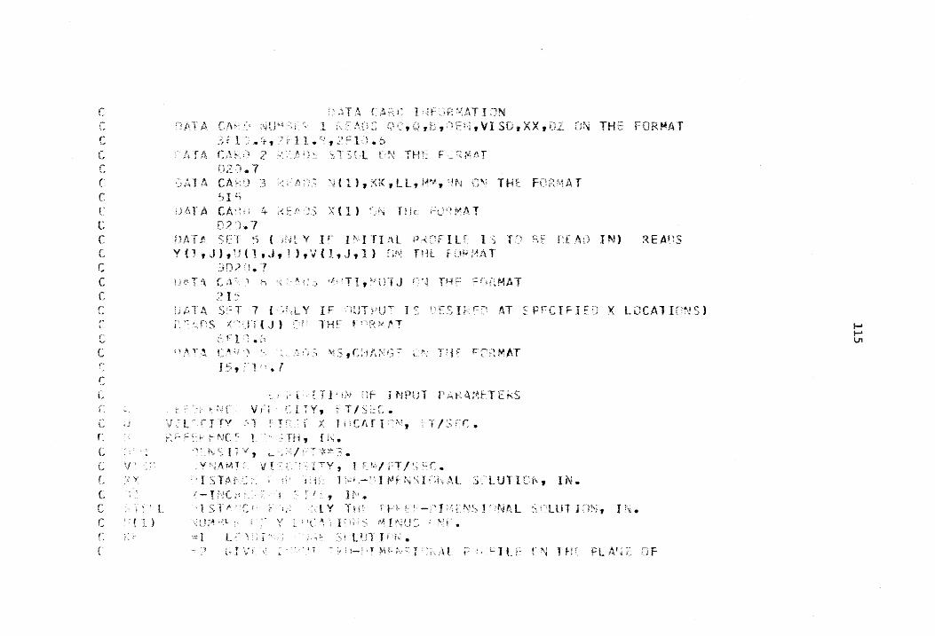
C \ .. C C L

(

C C C r L

C C C C C f~ ,

C C ,..

(

L

(~ d

r. C C L y

C r : .' 1 "-'

C f ' {

C C

> ;~ T /\ {',l~ r; I; ,!f_'jH rl,AT I IN r.·:/',TA Clh' :,~U~~ 1 :\t'i f.) ,~., , F ,VI Su,XX,i)Z {".IN THE FORp..iAT

it .. ~'r, !~ or A C' ,",,;~ .:}

,> "'-, " ' " ("-

OZ).7 ·j..\Ti":.. CA :J

:;1 ~;

l- 1 1 • ",' t / ~ 1 J • b

i~ i) ,"; T S 'l fN TH F j''';/\ r

Ie ( 1 ) , t~ K , l L, t~~~" C,t THE Ff~gft1t\ T

!\1' A C /:.: ~ i 4 >< F /. • ~;; x ( 1) ~)~ THe i~ r~ A, 'T 0.1 .. -,

f} t\ T ! SET 5 ( i H l Y I r I!-' I TIL P.( [: r I L r 1-; T r: H f r~ fA !) IN) ~ EAt) S Y (1 , ,J ) t U ( 1 ,.J 'I 1 ) , v { 1., J ,I} LI\; r H t f i) F 14 A T

3D? .7 t~ T .~\ (., .~) ') l:'i '~" - :, .. : ~ ~) '~TI, U'fJ r:'~ fl-l ;:t.i~MAT

? I''; illA S~:T 7 {':'~;L Y IF ,';uTruT I'::

i'. ~: < f: S l ,'" J T ( .J ) : T H r I ~-, r .... I.' r T r'l: .. ~;

I ) /'1, T.~ C i~ " t. ~, !\j :~. , C;., 1\ ;': I; 15,:ll .. !

- J'.i

~ .. ,';

[SI ~~ AT SPFCIFIE

TH~ l::r;~MAT

;. I ~ T I} L\i f~f J NPUT PAt,',AJ'1fTEf.-:S i:- :.! V .; ~: I ;- Y, i- T/S;:~: •

'J·:L i-lTY ,',1 !,T'r Jj Ct\TI"~\I,:"f1 F"r:. r.: c,>" !\!C r. '.~ TH , f i\. '''l\. ~~, I \/, L. I

T ,~~~,~ ~~ • Y~'~,Ar"T " \l1~' .~ I"'fY, 1 ;:, • .-,/ fT /S C(".

> ! S T (.l r :' . T ,- "; 1 ~~ ~ ;\ I !~ l. :) ~" L UTI C)\ , IN. " - I f-,} (, :-' j :;, 1 f; •

x LLlCA1Ir:NS)

lSTI',"f> ;-; :·.lY TH'; fr l . -:"J F\L<;;J'tNt\L :~~->lUTjn!\h 11'\. _;UiA .. ~L: 1'- '( . "i; I '> ;~,~ U~U:, ; ~/r ..

'·::1 L ,\'; i ,\! l!,IT Ji • '~ J \; t. ' IT :t ! I-! 'r ~~ f·.·. I' :\[,. ;':.:; ..:: 1 L ! 'N 1 r 1 z. P L A~~ ~:: F

I-' I-' VI

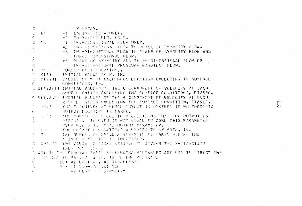
c C lL ('" 1..

r ~3·\. V

c C r t"

t (' v r \~

C X(l.)

C YC1,J) r C 'Jtl , J,J) C r V{l.J'!.)

L

c ( " -, ~

. I,..;

(.

r. 'I.

r 'j

c C L r

Y/f'l Y. =1 L .,!\;' i F\;LV. =2 TU-< Ut :::-

1 ; 10 f·1 :~ l FtC w rn; L Y .. ;;;:.~: I,\:tIL Lf:;..l Tf; f/L.i\\'t: ;-"cF SY~MFTkY fLGW. =3 l' ;-;~,U ~iJ!~,. N ~:l l):'1]:\ L r l e\1.,: IU P ltd'!E elf SYNMf. THY FLC.W AND

T(-a'~L t::- 1 P'S Ir~NAl flOW. :::4 Pl!\tJL :t v;,p.J<rTRY iH'iG TH F'~-~)I~'"E IPt\,t\l lOW DR

T ,"-;1 '.-t:::Lj;\',~L P~r-:SS:}P'::~t~qf:NT rLU~y~.

J\IU i~~ (, r l t iC 1\1' I (iNS. J;'~ITJAL Vt\lur C:F X., IN. V.dlUt's 1;}';: Y ;'T El,CH tiCV I

:. L C;\THjN EXCLUDING TH SURf,\Cf C;\NDJ11 \'St J:". INIT! :\l V,,:\LU F THE U (:tHAlP~ r~NT OF VEtr·CITY AT ACH \;1 fiF l {c:~! I ;: X C L U DIN G r H r sup rAe E c eN D J 1 I DN ~; t F TIS • .I \' I T I ,. L V L U (iF THf V C,: pr·~;~r- '·,-r Cf VElCCITY AT fACH \" r: t T \ 10"4 FXCLnJlN(; THf ~IY'f-~CE: CCN~1ITICN., FT/SEC. fHf f~.·: 1..,i~JP·~CY T !-IICh UTf';.rr I:;' SIf\F IF f-,hi SPfC!fIC "JUT PUl t~A~')' r:. Tl,H r·; r· CI fIr, L~'C:~ f1 i.'i-J::-; THAT TH UUTPUT 1 S

tl l' T J IS f\r:T Cl~td_ T:I ZERO TI-HS P4H.~f~ETt~{

" v;;.. r:i . fA 1., r I Cl VT F 1.1 T ~.) :~ A ~ F T FR. r ~ u r x L) C,~ T I !1;~ ~ fE, f :::: i) T I i Y 114 C 1 J., I\!.

;1 i' ,,~u tl':~

>(- I N'- . " :-j'

";1~tLL X TU)<:. T::1 r- TAKf~~ B Hn<,~'- THE: :. 17 I S J NC F.F 1.\'- r.:r.

T PL V!l.L{} r l;i>I:~. r::: 1 ~'i Tl j; VE T'i::- )(-'"' i. . (: I I ON I ;\ c~: i\.' T -' .f

C ;; T r ' I T i-: P t>: : :;;. r i-l F ~ \ H: ~"c I j';C· lr:": Af~ US~: rft >':1 RveT THE r ')

....... ., ~.

L c

1 ;' '. V;\ 1, i J:~ :S' c:·: f T f,ti ,.J ~

Ll 'i :: 1 t J '<::l, , =7. 1 t:Uf :--·If "::.: J T -', 1 ;. \0 S r .J.' \ t .~ :~ t.

=~} L.";, i< t .~.~ y 'J, :: T <,}. Y

v .

1-1 1-1 CI\

r r ,

r. [,

:-{ i"L\,'~< 'jY n: Y, T P ~:- ;'l{ 1'4: r.;.1 :IN:.\l PR~~; SU -]f." Y ':1

:{ t( f( - N tl ~! ". t ; f- l' C i\ L Z - II ': r. /! 1 I ,'!,!

I "1 P t I _ I T ;~ ~. l .* ! \. - H t ! '- L ) fJ'?" ;-1 r L' ( , 1.' ,,;. ), V C ? tln~.], 1 :: ) ., ~ ( ? ~ t;' ,1 )., ~'Jl ( r..: , 1 C~) , ? ), E : ~ ( I. , 1 ;., l

Il,Y! ,1 "),X(}~ (1), '·YX(·),V.~Lt.:L(l;(!),:~C,'.;, ,VI';;~,VISi~,r1 ,';.:\,1< \h~ , ~-( 1 , :":~ 1 \':, ~ L

C nJ'4 {." I N ( ? ) t ~: K 1 L L , ;·M.~ ,:\ N, KKK, f·j X f I. LX t UU:'4 ,,:', fY! )It~\C: ICr! tdl'" ~ ,'.dl' , .. ~),C{l;~,r')t~p{l' ),1')(1,1' )," (lO·""'.,)('lUTL>(\)

C T TTl AL I 7 .'\ T I' . r, t f T (p- V J.\ ' IOU ~ i.'" :~n '.' {' ,~C \';0"1 r -= 1')

i~ ~ \ ,~.~. t ,~ f':"~.\ ::: !"'

CALL l.iti :.,-:-.\ ~.:: i\,:(';;,1";"i') v;::TI"p';TJ

4(';i" F ,;~r.j!AT(/I5) 1 f· ( i J • l-~(J • r·)' T i J l1')

: ,.\f.; ( ~5 , ,+ 1. { ::U T ( I ) t I -= 1 ,1'" (':1 J ) .!+'\ 1 r ' \~ f, T ( 6 Fl. 6 1 4 ? TX=l

!\i(?) :::\,;(1)

j>~;lL .:UT;JN[ ( I X) 11 C /', L L ;~;'- L T'~X

I·, ·1 "f-,.> "'

I F {'fF; T J.. f' i;.l } , ; : T ! i" I) 4 ne 4(: ,...I J= 1 t ~jj'r.}

)( T TT :'.;; x<~u T ( J J 1/1 '. I 1 !;; { (.?). G T • X 1 1 T ,. :~.: !'~:. X ( 1 ) • LT. X IT T) X ( ) .: X T l T C!rlT r\JU c

Ii"') It {: L L \~U \; T F ~) ,"'U~JT,:::"'CC'U"~T+ 1 17

r,i! +1

t-' t-'

'"

>,.:

'" ....

~.-I

'" -'-.. "':

::.:: .. ... ::: ~

<,.

:¥ .... lv •

,....! ', ..... II ( ... '.

... x< I' .!

.... " r-"I ':/ .,-,: -'

..... ' .. -!

....",,. ..,;:.;."

-i H '-I <'. i.'~ . '. 'if.:" '-'

If',

.-l

,..

.. ('.; -.;;.:-. ..

--

to

too

<1;

...,

:':) _J <t

..

.. .....

118

.. ,...-i

+ -.. J_

,1':', "".1 .~ ::s: .. -:!;. t ... ~ ..

f\j

;;:

C'

+ ':a::.

~;

+ r~,,~

A •• .. (\t -~:

:"11") ¥ .. ""'? {~) ... .~.

fo-':: L if: .'.1, . ...., .. ...J ':?" c.'t <! tn ---'" > ; ...... c. -, l.l r¥: 0. :> ...-.l n.. ..., !",) ~., f.::o.. -, 1..-' '.:'

Z " :::.:: too I '" .. ,..il\:i:.- -f\,! ,,', \\.l ;j" f\. !, C' - ~l !I ~,:".j I -, 1\ <~.., .. ;,: X

-, ~ :;:':

z " :;: .. t u .. , - ~2 to I '.LJ .. I:\;IIX.- '!"""I "NII . .:t

('.; _ - V] \'i ;:L -t • ('t.,J _ -:,/'1 11 '::: -:? II .. 1""1 C'i !! r:~ - :~::. ~ II :;-'. <.r: -, '""':1 ..., II,"\.: <:.! .. 0 • --

-,

:') -J

c:t -r.~ ~

~~ >-.. II !-. f\r - .::..... II !::t.: J' -

» ..., .. t,~ -, .. -I -, .. i- ~: ",oj' ....J 1:.111 "'",1 i- ~ :- --" 7? ...; {(~ .. .-:

-J r"·l ....,...; r.1' j,~ ~: :.::

,~~ ....... l.l...

~,-

...J <l': ~ .. ...,., (3 !'-

£

!f .

--...... ' ,.~~t: c.... <J /'" U r',_ 3i I,,";

.(" 1'-

£.",

:~ ..... +

)"< t-, .... I- 0:':' ~" 1-; =;

f .. r.:: l:o.'

<t t.;,' U Lt: £ :r 11

i ... J

L:

If( ,)C»'{f. ::.11 ! ! I 1.-t .J'. T 1 ?

l"t C 'lTT "H.JC C :J,tL!fj I, fHICK ,:~ L iIi l'l\i

j' J l;'. 1 1<::.:.1, :< '~. I « .. ' ::J g T ( ( ii ( 2 f ',~ ( ), v~ ) * .... '! + ~~ ( ? y ()>> t j( )tL'j( / ) I( U ( ? .. '.~ X f ;", ) :;. ~<? + ~ ( .2 • ~~,X ,

1 ::" )). ~ T .:). ~l {~ .' I ; ~! T " 1 ,"l ..

, 1 <. "T J \': J L

C f-XP;~;'iiJ<)N Pf- 5fiLUlld\l rHl(K:.JF~:)S

Y~'~/tX:::: .' .• ' .. ;n*v ( :(, fT,\ ) ; )~'. 1 ;; .. '. J:::; j\!X ., 1 Y ( 1 t .J ) :::: Y ( 1 ,J- 1 ) + ( v ( t ~ J -1 ) - V ( 1 ., J-?) ) >7- 1. • ;}6 y ('), J) ~~y ( 1., J ) ~Z(2,J,1)=Wl(2,NX,1)

7 ( 1 • .J , 1 ) :::: W I ( l.,;·.f X f 1) ~n:::.J

I I- ( Y ;!~,o X • t T • Y ( 1 ,J » G iJ r n 1 2 l:~j fe: T I'~ U;;

~.1') I T ~ ( 6 , 60 P ) 6>', F;,:,~1~Yr{lX,' SlllUTi \l THICl<Nt~:S'; Tf; L.4RGE')

Ge, r 1 18 L(~ N(Z):-=.jT-l

>~P::::N ( ?)

NX=.JT N'~.J=N(l)+l O(i 1?4 IP=l,.? !X.: 12 l t KP=I,K\ LiI} 12 l t JP= , NX

( I P , ,I p + 1 9 ii, P )=;::~ :\#, ( I'" t 1 , K r) ) U {IP"JP., KF )=U ( H1., '1'21 K?) vtIP,JD,KP)=V(I0, ~,VPI

~'i~{i? .,.,fP .,!<y):::::>~( I "

..... ..... \C

1. "i ,(~ r;. ~'\j r 1 '.~! J ~. ;,; ( i ) =.; :,! C< )

1 - '< IF"<~(j rJ .. )

1:-':,:::2 ~f'; l"'ll JJ=l, 'I:~CT J Xl T T ~ ',C1 U T ( J J ) 11 :. I

1 '{ (: ")

I j- { X ( ). r-.r:: • X T T T ) T r~ 1 0 C· 1 C,,~d L ~)!j T C:T'-!f ( I X) ;;,h IT"{ iJ, l'fl) ~}C' 1, r'~CiJUNT,!\HJi~F,[ ,"'1Ci ~u NT =','

1 f' '1 1 C t ~ N r I'j U r C" 'I; 1 Lt ?

ton If(r·1CG;JNT .Lf .;4U'f I) Gt 1 TD lLt? I X= ') CALL uU TeNE( IX)

f.: IT ~: «(;',1"1,1) NC'~U\:I 1 ~"'CUUNT ,NU~!tHJ\

14 1 f- U R i'-' {l T ( 1 X, • I'JC <] H~rf =. , I '3 " ~c r U ,fI-,:T ::. , I 5 , • :'~CUUNT=rl

C S :~;;J :: N C I r~ flO G I C 142 l~(MMX.GT.l) sr 10 16

J r P'I i>i\ • ::: Q. 1 • [~N C: .. X ( ;.,,: ) • G ~,~ • x X) G G TOle IF (X (2 ) • LT. X X) Gr~:. TO 161 I~ ("1~b. Fe).?) 1I~~'X=?

IF(MM.~O.3) MMX=3

NU M a f ;~= • , r 5 )

C Cji.~.~,iGE OF SCLUTIC\i j'::i<l!'-' TWC-JIME~:SIC;-JAL T'J THl·U:c CIM}~;';JSI~-!NAL

KK:<=NN IX=2 CALL POT{IX) 0(; 1:; !( :::: 1 ',_K K K U ( 2., 1 f <, ) .: :) • ;) v ( .~ t 1. t j( ) =0 • we ?.,1,:()::~~. J

t-' N o

'i ( 1 t 1 t !: ) ::.: 1) •

V( .~'t l,l<:,)::::..:.

W(l,i,\):-:.u. I f ( • '~,f .1 t S '~- 1: 1. j t ·~i!( 2,1,:<.)=:'.(' ;4Z(l,l,K)::.; •

1 ':! 1 fl' 1. J:::~), l't.jY ...

U ( ? J J , ;< ) == u t ? t .J t 1 ):qH ? t ;TK r 1<) I U ( ? , ~). , 1 ) V ( , J. " ) =V ( , ., J , 1 ) *U ( ? t I,! X, !< » I U ( ?, ~) X t 1 ) W ( ~ t J, K) :: W ( '-? ,\~Y , F) ;J ( 1, J , !( ) =U ( ?,.J, ) V(l,J,K)==V(?,J,K) W(1,J,~)=W(2,J,~)

If(K.GT.l) ~G TJ 15 WI(2,JtK)=Wl(2,~XfK)

Wl(I,J,K'=WZ(Z,J,K) 1") CLtr\.~TIt':Uf

Nl1j'ti:Jt {::l

c r: 1 ~~ I P = 1 , .2 DOl?::: K.:: 2, KKK C ;\lL S tir .~ ~-:z ( I P, K )

1 ")2 C ; .. Nll ~\jut= C STGP?I~G CRITE~IUN

16 IF(XX+STSGl.l .XC?» GO TO lcl 1 !~ 1 I F ( U ( .? t 2 t 1 ) • t T. • ) GO f n 1 8

(;0 TC; 17

I V --) /;, ---.'

IF(U(2,?,1).lT.a.) IV::] C/\LL GUTC~! f ( 1 X ) \:Vi' I 1~· ('::: ,141) \<C Hh1T., !V,C:3Ut\iT, NU~ S l-'~ ;.

'"'" N

'"'"

::;U (·UT I Nl' H'!~r:,

I ;'~,Pl ~ r:: IT;;' AL'~;J ( ;~-; ~t n-l.) ( j , ;' J ( ! 'I 1 :; t 1. ) t V ( ,;' , I. ., 1 ), :-'V ( ? t 1 :' ;:; ,1 ('I) ,;rJ -, ( ? , l I.'; , ! t .'. ) f "(:}, l :1 '.~ t 1 ,'i

1 ) ,Y ( ? , 1 l"; {} ) ,X (:~ ) f Z (l ) t ;.;U: V X ( 2 ) t V pl U F ( 1 no ) t iJ C), c} , ,V I:j K , VI S [.I ,D L N ., ;,( 'f ;.'

'If2 V . ., n X 1., STSJL ( : n ( 2 ) , 1\;(, '._ L .,i1'~ t r\J 1'4 ,. K{~ . ., ;r.~:V: X , l t. X , NIJ ;··FF· H

C T!HS ~~U·~.f-::"jUTINf ;:IT~'F ;.~C;.'i~~ IN f ~;l,'\'.:(rING }l;lJFIL IJ;~. ~::;Cl\H":;{i\TfS.4

C rH .. ~.H:':K \.~;.~ IlF F~JR Trf L~'-Ar',!:l(; Fr'c~- ~ .. LUT!GN. ;: ,:\ D ( ') , 6 n ;1) Q ) , ti t 'f:J E 1'.J , V I S D , X X., .l

~~? r T!:- ( (~ ., 6 'J 0 ) ,}} , i::, , U f. N., V I S D , ).' X I 0 I fH'-~ h ,R.M!\ T ( "-) i:-: 1 O. 4 , ? 1= 1 1 • ,;; F 1 '). f;,)

Ai)( 5,6Qf';() ST::CL 6010 FQ~~AT(U20.1)

P fAr: ( 5 t 6,J 1.) rH 1) , fZ K , t t ,I<i M , N N WRlft(6,6Cl) N(l),KKtlL,M~,NN

6nl fDRMAT(SIS) lLX=l ~H-1X=l

KKK=l I F elL. !:Q .2) t L X= 2 IF(M~.[Q.4) MMX=3 IF(MMX.f~.3) KKK:::N~

iJ.= B/1.2. SlSGl=~TSOl/E/l?

XX=XX/G 112. Dl=DII (12. *3) VI S.K:;::VI SD/OE'N ,Fvr~=:J O*B/V I 51<.

WRIT [:(6,6(3) V ISK, :..!~tY~ /)").3 r: C H~L'.ll ( ? D2 0. 7)

f"~X= \1 ( 1 ) .... 1 IX=l

.... N N

;: ~ #\) ( '). 6 n 1+) X ( 1 ) 't ,'< ,,' r (\ • 7 )

R. F Y X ( 1 1 X ( 1 ) / V f ''.;( /1 ? • X(l)=X( l)/;i/L?:. Y ( 1 ,1 t = .:'i

Y{2,1)=C. Z(l)=''i.;;

fJC 1 i<.;;::;? t l"f' 1 Z(~}=l(K-l)+0l

~~<t(=l

I r (;:"'1 fl.. f Q .'+ ) 1< K:;~: ~,l

r \L :}C t( Pf<pt::! L f ? '!.= 1,:: l<)~

U ( 1 ,,1 , K ) =[i.;)

\j ( 1, 1 , f< ) :::: i). D

\IV ( 1 t 1 , K ) = 0 • f; U ( 1 ,NX , K ) =(;)/

V( 1,l'D:"Kl=G. (' W{l.NX,K)= .n I (~<.(;T.1) GO TO Wl(l,l,K)=O.O I"iZ(l f~\J'x:,K)=i).J

Z G C!\.!J I ~JUf': !f(~M.EQ.4) C~LL ?8T(IX) IF(KJ<.. .2' GO TO 7

!< .. l,.)=N (I ) DC 3 ~':= 1" ~.KK Dt' 3 J=2, U(l,J, )=U(l,NX,Kl

2. 1. V ( 1, J t 1{ ) :: ;'\ • ,) W(l,J,K)=W(l,~X,~}

IF(K.lT.?) l(l~J, J=WZ(l,NX,K)

I-' l".)

w

3 C i ~.~ l I \1 U F f:y:::;, .;;i' 11 ( *1!".)~: Li ~T ( ;:y;:) ,'" {:j J:;;; 2 t i,; X ! f ( " • r:T. {-,) cn \ r.";

Y(l,J)::::Y( 1..,.1-1' t-i:" y ( :~ t J) ::: Y ( 1 , J ) f',{J TfJ 6 1)y.=r;Y:~{l • Of)

Y(1,JJ=Y(l,J-l)+0Y YCl,J)=Y(l,J)

~.) C Ci'~T I NUt Gt, TJ 1

C J eUT PR::FIlE 7 i~: J=?., ~JX

C U( l,i1X,1) ~J,UST [C!li"i':lISL:~rn WI fH prTfNTIAl FlUL~ ANU YII,J) GIVEN IN C. I7\jCHf"~: WIT~ lH~~ V~:l';(IrlfS GIVi:N H\l rT/S;:C.

Rf [~D ( S t 6(2) V ( 1 , J) , lJ ( 1 , J ,1 ) ., V (1 ,.J., 1 J t)('"~ FCH~_}" :~T (3D20. 1)

~(l,J,l)=W(ltNXfl) V ( 1, J) = Y ( 1, J ) I { :>~ * 1. c: • };it n c~ QRT ( ~'~ EY ~n Y{;!,J)=Y(l,J) U ( 1 , J , 1 ) ::U (1 ,J T 1 ) Il~': V{ 1, J, 1) =V( 1, J, l} -~<; 5 T( HI «(,)q;t, VI S K) 1

q Cf;NT r'HJ [ :; ;{=l, Ki<K

0:1 9' .J=2,rrx U ( 1 , J t ) :::U ( J, ,j t 1 } ,,~ u ( 1. , :,1 X., K ) / U ( 1 t ~,: X., 1 ) V( 1, J ,<.) =V ( 1 .,.J t l. ):<J (1 , ~\:x, K ) I U (1 ,~x ,1 ) W(l,J,K)=W(l, X,Y) If (K .Gl.1) r;r': 1:-1

I.-J (lfJ,l)=\t:Ztl,~~X,l)

9 C i", ~1 r 1;'-1 U

I-' N ~

..,..:

II X .-(::4~

.....

~:. ... ''(', )I

... ,~

,.... <i.'

11 u .<

t 'i

-i ....;

'-." ~

~- . ..)

125

" i

::) ..' -i.

r.-" =l ~;~ 10- -:-. 1.1 .. : Z t..) y Lt..i

!""I

~

!.J~'i<l!JT I ~\l~ peT ( J ;0 J \; ! J C JT ;:;.r!.\I·\:~;( ::,-~\, i.i-L)

C :,>,>; 1\: U ( l ,1' ,l;}, v C ._' , l' , l {\ ) ,~~ ( ? ,1 C';! ,l ), \r" 1.. ( , i. J , ), ;.~ ~,~ ( L, 1. ~-. ,1') 1) , Y ( ,'. (vi) , X () ), ::r ( 1 i) t Y)" ( 2 J , VA L lH f 1 (i '1) ,QC ,P tnt v I f V I '.) ~ \ , 0 EN t X X t H 2. 0Y t ex 1 , S T lJL

C ;.~ (\~ N ( ? ) t ~,! t , '.; '1 , ~J N t ~: K K ., r;. riX , t l x tNt, M G l: R c r H T S \i.hH::.n.Jl I~f [- CL C}JL'\ T 5 THF PDTFf'ffI At- FlIJw F c.'~( /~N IMP r NG I N(; Jf: T 1\ T C I\NY X-Lrlt~T I Dr'~ I~lr:.dj:", TH /-.t\X IS

\; ).=?-": ( I "() "·1 ~i X ::: \j ( I X ) + 1 '-t-JvJ=i) ... ·~

UU::;:;U(l,NX,l) PI=3.14J59?b536 1\=2. 75/B+XX U2=UU·!t*2 W2=\.-iW**2 EPRO'·~=1.1n-08 [ii] 3 K=l,KKK

1 F = -P 1 * ( x ( I X ) - A ) - (1 • 5 * D L iJG ( ( ( 1 ."U U »* * 2 +W ? ) I ( ( 1 • - uu ) * * 2 +W 2 » ) - 0 A TAN ( ? l*UU/( 1.-U?-W2) )

G=-P 1*( Z (I( ) ) -Q • S *DlPG ( ( ( l.-WW) **2+02 ) 1«( 1. +~w) **2+U2 • )+D.4 TAN (2. * WW 1/ ( 1. -U2-W2 t )

F U::: - 2 • ;!,( ( 1. 0-U ;: + W 2) / ( ( f 1. 0- U U ) * * :: + W?) * ( ( 1. I) + U U ) * * 2 ... k 2) ) -? • * ( 1 • (' - W? + lU2)/I(I.O-U2-WZ)**2+4.0*U2)

G \'J= 2 .. * ( 1. 0- irl Z + ~J .::) I ( ( ( 1. 0-" W ) ** 2 +U 2 ) * ( ( 1. 0 + W.,d * ::; ~~ ... tJ2 ) ) + 2 • * ( 1 .0 -U.2 + lW7'/((1.O-U2-W7)** +4.0*W2) fW=4.<~UU*~-lW*( 1./( ( 1.-UU)~o~~~+W2.)*( (l.+UU) **2+t.J2) )-I./( (1.-U2-W? )**

1 ?+'-t. *U2 ) ) GU=4.*UU*WW*(1./(((I.-WW1**Z+UZ)*((1.+WW)**Z+U2))-1./((1.-U2-W2)**

12+-.t.*~2) f;u~-gU

i3tnTU~\~=fU*Gw-Fhl il:GU

.... N c:J\

:c ;f' e: :-: """i­~ ,.. ..

" --

f'~ -r.. ~f-

::. Ii' ("'.j

:::;

r·~

C! 1-"

C)

!~.;r

~'

"

• l--J •

l' (,)":

~ •

~-;. 1=1.

• '. ~.

r-_1

t

u.~ - -I~ -~,~ ..... t .... ~

!'i1

C'J ..... ~J \., x X • C/'J

u.... • -t',J

x, • ll'~

• :;.;.< :x: )I"

~,",:~, --

127

!""1 .. X Z .. X ..... -:::> I .. ~ -* •

...-.4 't-'y.', + -+- '" .:::at::r:.: -

::; :3': ,;;(' .. .. Q..

~:::: XX 1/ II " • Z Z --.-I.... ...... ~ ~ ....... ~ .. .. .. C~ I , ::> :~: u..; X

Y X n.; X >< ::;, :r ::> z :;::: :i:.~ ...-...... .~f- ,*:2 .. ;;;::: .. "'<--:::J :,.::;. ...... Xtx,

XX_;::,X:::;-;:J: ...... _~ _ ...... - H II II "Z-~C:: - - '.1- ;,., 3: ~ N C N Lt.l ;~: :::::J 3. ..... :.l:::,) .3: U ,3:; :(. u...i

..

.. ...

.. -::;.. .. .. '"

.. ':;', .. ...

'­.. ,"

.. > ..

.. -C >::: ::,: >-

",. ... ~ t..~,;

, . ...,; .. "Y.'

) --.. .. > ::

-r"'" .. ,.._t

1-

.. .. -...J '., <'i JI1Il" •• l ><

~ .

-', z: ~""-.i .. ->< J: -' -J" .. >< ~­~:, ii"'

",J;; ~l 'U"; ~r;' ;Z' .. ~ .. ,.:-::

~';: ~ ~' .. - '''.:4

~< ; ~~: (-) ..

'" .... I.':' ['.J I- C"',! ,'i."" -

c'< ~ __ lit ~~

..... ... "

I-;~:

'::!

... -/) I"'-'1':"

• I"""i

'",1) <:;. ~1",

128

•

'f" ... .... '"'

• •

l-I

• >, • i.i. l (';

It

\0-- :~

Vi

It

•

<.: • )<

l.l)

-.::-,....~ ~~'t • c_

.....-I • ~£- ~ ,....~ ,,~,

)( . C.>; II :," .. a.

It

Ci" .~~" ,-..... (") "t' l:J ~. ~r ' ,,", _, ....., • - I". • ':'!:: ':< ...... ..... t- ""'" '.I I- I-

;;:: ,., >< .... cI -1 t,:'- C) (! . "" .. !".......... + ;?: I"""l It X C" •

OlJ"l ...... t"';::' I-~"''' .-:;.~, I. !¥c" ..... 1-1 i.t"; .....:...... L,,, + I"""i ..., 1 U I' i C: Lj, '1,J ~.~ .. _ ~,:J.; 11""'(1 ~':'''l .. (:::">.1 ',I'; ~' ....-! '7)

~r." ~.~'" \_ ~.... f' '. ')t: r ..... '~ "'''1 ., ("', /1:"'.1 t\,~ ~~~...... • :~- I :., >:; ,>,' ',:> .~'~.; It II (', - '-"" _ :':':X: ~ -' 'I) ....., II II

II ,'I"': ') ~ \-- r ,.- 1::2 Z ' .... 3 ....,. -, J- t- >., Z' l! :-.~ ;;"':" ,;;,~, ;;:; ::,":" >- ~J.: :.t:. .... ':~:. <i; ,f. I,c~ II ~. II 11;';: II - ,....j ..... _11 .. >- ," :..-/ ~ ;.J,.. ,_ '.If'. 0)(. U" t-. CJ ~" J.. >( w.. !... -, li,. r-- r" X ~:J IL, P·.: " ~ .- "-~> ~J _ ...... ,:,~, ~ _ '~: l-i ...... >: >< ...... tq

, . '-"

(:, -(.1 t: ...

t/

.:::: to"",l

X Vi t:.l l-

'* vi I- +

I"""i Z X :..( k!..~ X ';0'1~ ~~ fI ...... 0.. ->--: ....... ('J

i.J.< (:.': )of, :;..,

-:2:::>< - <! II -....;X--l .. U N '::'-:' x+_v: .:.::. - >-~- t ", .. ~ ~/t ..

~'\A - - + - X >:; X ;::.:J II ><>< ,_ ~ t

- {\j 1- t­,-; - '''';': <.!' .. X • til

~.: ....... ....-~'~'." ~ r'\ ~

... ·A~': -­"'''~ .,,~ )( ; ... ,~ - ;-":: . ~ ;.:.i

'"'i :r: ~"* ;:~', • u .... -:: <.r

.-; . . .. - t- 1"""I,....i (,1'1 L') , It

a::: • (t 1-­<1: r- w,.; ':.:.: t::~: Z • • II I~.! >,' ,< ;:.:;: I- U !::. !:: r..t: ;::;~ O~ .~: ::;: :;,

...... --l-:::­Lt., !.-J... ~h:'" ,~

~:t. t-t '-I -

;.r" .J.)

129

i~ I h. (Iij r T t !\; l S "' P 1 P L I I T i':;' \ l * i:: (,~ - H t n - z ) c : ~M·~ J i it? ,1 "', ~ 1 1 q t V ( 2 t 1 '~~I ~ 1 ." ) ,~~ L I , J . \: ' t 1 ) t ',L~ ( ? t 1, , ), f J! ( 2, l' \ ~", 1]

Il,'!( .,1 \)),X( ), (1(~).,~:~ YX(?)"VI1LtiF(lcn),Q0" , ,VISK,VISi),OEN,XX,; ? {. y ., Xl, T:; ;]t

( \- ;,:;., N ~'( '2 ) , !< ;< , L l f r-~ ~ , ;~ , y.J( K t ~'l,f; X t i. lX, t-;u .,/, 3 ~ R C T:~;L~ i~n-~:i.;.cUTINf: P'?t";Ji·C1S l"i~~W VflCCITY pP.C'fIlFS AL l1',;G TH 7= ~jEXr X-STiP t h {ij I'j T Hr l: II L ,.J! :yr I r::'..,) ;,\t.l,y~{~ T HI:S :~ FW L n CAT J f'f',l

r: 1:-;;; f (!) of, 1 .! ( ? ) ::::;. ( 1 )

F'.=:.~' (',) ) L ~ V':'· LTV .-:<:

i: ( '.j L "!, ~'~.' ..~ l ! . N j~: ~:/

1 r, (: u·~ \' • .' ; L { V F :;: 1 t I(:!. 1 , ::.;,

, ) l' ;.} .J ':"_' 1 , :' .. : }t (L ; \If , ,I , r- t .:: f ;.~ (i 1 \F. , J , i<. »

U ( L .J \: ,J, l~, );.; I.. ( L. f \/ t J J " ) " (f . ;": V ,J " ).= \;( t I V: , J t ]I; )

t~ f i V r", .J , f~ ) = W ( t I V , J ~ :( ) I F { K • ;;':~:i • 1} W l ( L:1 V , ,J ,K )::: W l ( L I V t:, J. K )

1;) GC;:; TI 'HJi= I F ( 4";:; X • • l) GO f;:'~ 1. 2

I CALL POTt I Xl

i 11 K= 1, KK K D;' 1. 1 .. I:.: 1 , N P U ( ?, J , '< J ::: U ( ~~ , "J , ;<.) -* U ( ? t t,~ X t K.) I tH 1 7 ~: X f K ) lr(~(l, X,K).fQ.· .~) ~ TQ III h ( " , J, ):;: W (?: , • .1 f r< ):;.:~: ( ? 1 f': X ~ K ) I "tJ ( 1 t NX t K )

1 1 1 I F ( ~.J 7 ( 1, N X t K ) • E • • • 'J • l(,. G T • 1.) (; f' T (-~ 1. 1

..... ~

~ .. X ~,;~.A ... -'

1',

~f::. ,~ ,:;e; ....... tt: ;r.

1-' .... " > ::> .. ....... ....... x -Z -' (,! .. -\,'V .. " ti"_ X

:'1:- -!} t'.J ::r * ~,

4'"~ ,'''''.

:::'I ,-1

'V ~/.

...., -< ... .. .. ,.." X ')-~ ..

'7"·

"'" .. .. :~ ~.

-''':\ ;.~~: ',I.. II II .. ::-..., ;:. ;; .. ...... r:"

. ,~

131

{PFnUrIN~ CL; Fr:{t,.,S,~·P.,C,i.',¥}

1~?tlCIT RrAl*f(~-H,O-l) (: \ ~ :·-HY't U L: , 1 1.: '1 , 1 ), \I ('t: , 1 tY ~ , 1 C ) ,W (2 ,I 0 f) , 11 ) ., W 1. ( L, 10 () t 2 ) • EM ( 2., 1 {) (), 1 ()

I. ) ., '( ( 2 f l:n f X ( ? ), ? ( J :' 1 ,?, Y X ( 2: ) , \I.~ U r ( 1 ,""\ r), ":f V I S K t V I S LtD EN, X X ,R ;~ .. y t '. Xl., STSl)l (:\ifi'i[~N f\l (2) ,t':.r~ ,ll J ;"j"'j fr~:~, KKK J r"~MX, llX, r~UMt3ER

I :~ ri,j S. If;:, ( 1 ~! n 1 , S ( 1 0 ) t !V~ ( 1:) rn ,c« 1 00) t 0 ( ;:l., 1 0 (' ) c r I :::.ILi::n:.:UTI:·;r rILLS U? THETFI-CT .!ll';Li"!f.~L ;'~ATRIX fOR CH Of lHE ( i~:~ •

p=;; (:?)

:< :.:.-'~ c: ) +] t,::::

C{.GT.lt t=l C r.:'.. i C ~"M C;;.:' /U) I !-!\H S.

Li ' :< ~ ( ~ J ( ;: ~ !" LY, , 1< )t U ( ? , ;'; ',< 'f K - L ) • U ( 1 , l\ X f K) + U ( 1 ., N X , K -l) J 14 • ';'\;K::::(W(2,~JXt;;)+/{ ?,i\:~~tK-t)'i'ir:( 1,NX,K) +w( 1,NX,K-L) 1/4.

f· ;li.X:::-) • .5-* ( 1) ( ~; , i\;);" , X) -!J { 1 , NX , ;-( ) +f! (? ,~J '.( , K -L ) -U' 1 , ~:x , K -L ) ) I LX ( 2) -x ( 1 ) ) '1-:: . I • ? * ( It ( ?, 1'; .X .,:< ) -~: ( 1 ,;'~ X , r- ) -+ ~t ( ? ,!'>i X 1 K -l ) - W ( 1 , NX , K-l ) ) I ( X (? ) -X ( 1 t )

I ; ( ;< • ;.; T • J) .:; L T ("j :. ,

--. ':. "; ( N / ( :.' J ',,' ,\ } '- A \1, i-~ / , J.\ ) ) I ( '( «2 ) -X ( 1 ) )

.~ ( .. ; l ( 1, .. t :" ) ,,', (. . " b;, ) ) I • ,. ~,

IL

'.) ,:.p,\i/.= .• !,*(U(?,'· , )-U{ ::',t.,q(,1(-!)+,U(l,!·iX .. K)-U(] ,NX,K-IJ1/(ZIK)-ZU<-1 1 i )

':-:-;. ~~;('.·.;{;?,'-'!·f'·)-·';(·>1!·" ~".-1). (1, Xt~~)-JHl,NX,1<-1))/( (K)-I(K-l l ) )

. T r j it

.. i . I "( ! j .. ~- :

.; J .. /, .\' '!'( )-')1(1)

- : l ~: I ,- J r i \1 r 1 T

... v.> N

; v j'::::: V ( 'J ,J+ J ) - y ( ,) , J)

'. v .'.~:::: y ( .:?, J ) - Y ( l f .J -- ], ) tF'= (U ( i: f J, K ) -+U ( "), . .1 f:~ -l ) +U ( 1, J, K ) t-U ( 1 f J f K- L) » /l; •

V :::; I V ( ? , J, Xl + V (!. ,J f i( -1 ) .... \i ( I , J , '( ) .. V (I , J • 1(. -l ) ) I -4 • I F (\1 ( 1 , J , ;< ) ,. F Lj .'; .':) \IF,:) • () * V iJ J

W~=(~(7,JfK).~( ,J,K-l)+W(1,Jf~)+W(11J,K-l»)/4.

I (;<,.::--;.1) _I:" ·1 1i('::.( (i( )-1.( -1) (; ux:;:; c.: ~~ (U ( ? f ~; , ,,-1 ) -u ( 1, .J, y. -1 ) -IJ { J ., J t !( ) ) I ;)X C~;·,X=:. >*(W( ~l"J, -'1)-"';( 1,J,j(.-l)-~(1,J,1<J)/r)x C; U;!=: .~~ I II Z i:'. ( l if 1 .. J t 1'. ) - ( i( 1 t J , K -1 ) -J C' , J, K - t ) ) f."~:;:::-. U. :; /I'l ;~ ( w ( 1, J t K) - (1, J , K -1 ) - ~~H ? , .J , K - 1 ) ) GCY=(,'l.YM/,.,YP'!!r,(?J(?"J+l.,K-l )-U (.2,.J,l<-l )+utl,..J+l,K-l)-U( l,J,K-l)

1 + U ( 1, J + 1 , K ) - U ( 1 f J , :<.) »+ i} Y P I D Y 1'1 * ( U L? ., ,J ,K - 1 ) -lJ{ 2 ,J -1 , K - 1 ) + U ( 1 ., J , K -1 ) 2 - u ( 1 t J - 1 ,K -1 ) + U ( 1 t J , <) -0 ( 1 , J -1 t !< ) ) ) I (lr • ~;~ ( D YP + L Y M ) )

G W Y= () Y M If'} Y P ~i': ( I,.J( ?, J+ 1 , I{ - I) - fd ( ? t J , f<. -1 ) .. W ( 1 ,J + 1 ,. K-l ) - W ( 1 • ,J ,K -1 ) 1" W ( 1 ,J'" 1. , K ) - ,H 1 J J , !< ) ) + CY PI DY f'tt {\\i ( ?, J , :< -1 t -W ( 2, J -1, K - 1 ) + II ( 1, J , K - 1 ) 2- ~'" 1, ... 1- 1 , ¥,- 1 ) ... W ( 1, J t K ) - vI( 1 , J -'1 t ¥) ) J I ( 4 • * ( D Y P'" C Y M) )

G dP YY .::: ( ( 1 .... E l"H 2 , ,j "-1 t K - 1 ) ) * ( U , 2 , ,J+ 1 , K - 1 ) - U ( 2 , J , K - 1 » ) lOY P 1- ( 1. + M ( 2 ., J , K -1 ) ) *' ( U ( , J ,K -1 ) -1.1 ( 2 t J- 1 'I K -1 ) »1 e V r.., + ( 1 • + EM ( 1 t J + 1, K - 1 ) ) 2 * ( u ( 1 t J + 1., K - 1 ) -u ( 1, J ., K - 1 ) ) J u Y P - ( 1. + f: !VI ( 1, J , K - 1 ) } ~:( U ( 1 ,J , K -1 )-.~qH 1 , J-l ., K-l) ) I f.iY ~'+ (1 • + F~~ (1 ,J -t 1 , }( ) J* ( !J ( l t J"" 1 t K )-U ( l, ... t, K ) ) IOYP 4- ( 1. + E M ( 1, J., K ) } * { {J ( 1, J ,K) -0 ( 1 , ~'-1 ,!<) ) ID Y M) J ( 2 • 4: ( CV P+ DY,~ J,) G~MWYY=((1.+f~(~tJ+19K-l)}*(W(?,J+l,~-1)-W(2,JtK-l»Jnyp

1-(1.+EM(2,J,K-l»*(W{2,J,K-l)-W(2,J-l,K-l»)JDYM+(1.+EM(19J+l,K-l)} '*(W(l,J+ltK-l)-W(l,J,K-l»)/CYP-(l.+E~(l,JtK-l»*(W(ltJ,K-l)-3w( 1,.J-l,K-l) I!)Y~~+( 1.f--EM(1,J+l,!<.) );¢:(w( t ,J+l.XJ-Wll,J,K) )/JYP 4 - ( 1. • + Co;'" ( 1 , J , K ) ) '* ( ~d 1 , .J , K ) - W ( ] , " - 1. , K ) ) I rlV~; ) J ( ;> • :.;.; ( 0 YP + n Y M ) 1

.ii( ,.1 ) :.;: { - ( D YP /0 Y l'-1) ~: V 3/ ? • - { 1. + F M ( '2 , J , w:) ) / I" Y fit]) I ( $) Y P+ DVM) I? • S ( .J ) =:i) :'~ I r:X i-V 13 ~~q ''; y ,)- ~~ Y ) I ( U Y P :1',- r, y V ;~:.) + t ( 1 • + E ('2, J+ 1 .~< ) ) /0 Y p+ ( 1. + FM (

12. , J, ,<) ) /0 Y M 1 I ( U Y F + i:: Y ~q ~(J)= (J)/2.+~8/. ?

t---' l.oJ l.oJ

t CO :: ( « tN M /l) Y :)) v ; / .', • - ( 1. • + f Vi ( ? t J .... 1. ,;f. ) ) I r~ y p t / ( :-} V P + D Y;><I) I? ;j ( 1, J) =U.1 i\} X* f u~,:'~ i· i'~ ;;\J X·~F IJ;~Z +GF MUYY-Ut~*GUX -\I F *CUY -W H *GU I

( ? t .J ) == U ?~ N X * r \'i;'; ,( -+ ,"1 )' -,:+ w N 1 + r:: ~ ~~ ~.~ y V - iY', * f, W X-V F * '\"i Y - ~ *' C ti l F;': Ti it

11 GUY=-~J(ltJ,K)/UX :.J'iTi = .. 'S I ( l)y ~) + f: Y .,.,) (:"' Y;." I:) Y? ~ ( U ( 1, J + 1 , K ) - U ( l t J , K) ) + D Y? I;) YM * ( U ( 1 f J , K)

l-tH 1. t .1-1 t K ) ) ) U'('f = ( ( 1 .... f;;-I( 1 , .j ·t-"t , f ) 1 *' ( U ( 1 f Jfl ,K ) -U ( 1 , J, :< 1 II UY P - { 1. -+f;'" ( It J f K )

} )i,.;(!,( 1,J,K)-U( l,J-l,!() )/DY'M)/(:,PfP+}Y;"') I'd .J) = ( - ( 1) Y ? / DY N' l -:t~ V L/ ? • - ( 1 • -+ [ ~ (2 , J, K ) ) / D Y ~ ) / ( D Y P+ DY~'" )

( .J ) ::.dJ:~ I L X+ \le:+ ( :') y;:.. -u YM) I (r.:YP *f'i yt,l;~? ) +« ( 1 • + f. M ( 2 J J+ 1 ,:,<) ) I t}V P+ (1.+ '::M (

l.'::~ , J, l() ) ICY~·) / ( flY P + 'OlY tJi ) C ( J ) -:: ( ( !~; Y M /:) Y P ) *- V I;, I ;:> • - ( 1 .... f;'~ ( 2 t .J'" 1 , K ) ) / D Y P J I ( DY P+ DY M ) ~ (1, J) ~unNX~~flH·L'<+i~Er-1UYY-Vf;*GliY-ua*GUX W!l~::::( ,fil (l,J,;(,);.~~I( 2,J,K) )/2. (:~! /j:, =-w l ( 1 ,J t K ) / L)' f;:,a,: Z Y= ( D Y M/ D Y p* ttL:: ( 1 t J.t- 1 t KJ - W 1 « 1 f J t K ) } + DY P I DY M * ( W Z ( 1 , J t K ) - W 1 ( 1 t J - 1.,

1 K ) ) ) I ( :? • * ( i~l Y P + D Y ~<) J (;f'~h'LVY;;: ((l.+Fi"'{l ,J+l,K J) *(Wl (l,J+l,i( )-wz( l~J,K) )/DYP-( 1.+tH( 1,J,K)

1) ( ~! 1 ( 1 ,J, ~q - \.Ii Z ( 1 ,J-l , K) ) I DY t-~ ) I ( DV y .,.. DY ~) P { J ):;~, (J ) +W l D I? •

D(?,J)=UBNX*FWZ~X+~ZNb**2-WZ~*Wl(1,J,K)/2.+GMWlYY-UH*GWIX-VS*GWlY

'" C eN T I ~~ U j:: t·~ ETU !{;~ E r-:Q

.... w ~

C C' f-; r INS h ( I X, K ) 1,I,?llCIT F1d,* (~-H,C-l)

C. ~ , '<~L U (::), 1 ;, :i "} , \/ ( " ,In ,~~ , 1 !",) ., ~ ( :' ,. 1 i) ,Y L?, It}r~),X C?)y (1 ), ~fYX(? ),Vl~lU (} !fYf;; .,DX 1, STSCjL

,1nJ,hz(z,l J,2),E~(2,lOOtl OltOO, , ,VISK,VISD,DEN,XX,R

c:-~ ii; [1 j -J N ( ? I , ¥~ i< , L L , ~'<;\1 , ~ L ~ , 1(,!< ¥ :f i'J; ,~~ X, L LX, N U M B F I~ C 1 '" ,·U9 , UTl~',;F :: .. At ~.}L. r:; 1 Hf: ;<~;IXlr:(; t '.GTH ANL"J THE Sth; tJ~~NT ft:DY f VI t~C SITY

i\ p::: ?:1 .. i)

;.: i\ X :;;; i;~ ( I X ) + ? .~ (I X , f4 ~ X,," ) :: C t(J:( =f'l ( I X ) + 1 1 f ( L l X. f; T. l) ( .... f 1 'f ill

eLf,.", { t,,' fL! iW 1 J=l,NX

( I X , J t to =- "; • 11;,:ur rIO

c 1. ", ; .lL, 1 F l {; ~> :} ~'J ::;'~ 1 (U ( 1 Y, !:{,':, ) ';: :;-:~' i'~~' ( .I .x , , ;t:) ;:.:) 1

'J, j ~:::.;; , t ),

,\. :<1(if(i"',.5 1 )'·*,~+;j(I;{,.J , )<;;;~. )/~·r

'. ~t '

J i ( • L 1. • ' 1 :) ~) .; \ ~

J )::',-: I

i,,;\-,l":="~ '~~T(U( JX,J'-l, ) *~·~+W(IX,J-t.,tJ') *))!tJN

y

w. f'\

Tl fl'

{i ; If .f'.-::V ( I., .1:< - J + ( it ' - ~~l ;,,: \4 ) / ( \) io,; - : )' '1 ( i, J X ) - Y ( 1" J X - 1.) } 'f =, i: " T ( ( ~~ ~ ~ ~ • (j ~ t ,'~

11 ~j-: .. :J, ,"

, f !\ ) IY f 1 j~ ,'> ) ) -;;,:;!c of ( h ( I){ ,,..2 f r, ) !Y ( I:t. , ) ~~ *~: ) T ( F !J~\~ C T ) 1,: !:; : .. l' .... i ~­. :.. ~)

f-I W V1

...

..

.. .., .. )to::. --~

::t: .. J"'"I I ..., ..

X -.:f ..

• c.'

r-..

--' .....

.. ~ .. _.oi '::.t' ,",', ;J.) :.,,":1 ~'l rr., ,-, *' ~t' • •

• C~ \".! 1". ", ,

' '''''-......... :. ..... - 'l. -' - >. t

•

• ;. ..... '* 1"- if'. ... ·i U~

I- I",' ",4" •

~- -.v: : ... )

•

..

N" ~,I

?; tt;

136

• I

5"',

•

\./~"t .......

-:-....... 1"

<~ "* ... , ojt

t-"j-

>-'""" , . -C' (\.1 >< C) t.iJ t-,

"" ):.

• it­<""'I \.1.1 - 't.; ~~ ..:t ,'" "'1) Co:;. )- . ~I- ,....: .... 1 'f (V'; X

• ~:- "':! C *' ~, --X ,'* ..-l II If' •• x. t-' t::'! • T ",',

.. " l,;:')< I )", "". >< ',~ "if' "'.>. .;~ ';,' L

..., ;............. ~., ~.t:. ..... ...,..~ ~., ,~~'.~ i,' >>> .. - - L., >- -! K, >- '0 ,_ - X

-- :"' -' >- - - .l., I.J, _. Ll, .)- *' <'t - - >-. + .,() .-I i: 'r:;/"~ 1..(';;:;: >- - + I- - • .:c- ~!. ::./ '" i.~ ...... '.;,' i',' X I - - - r.::: .., C, C) ~!. C {!' ::::: 'i- . .(.: •

.... t.... t'-: -, • .. • • ;.~;. ~.!.) ~~~ .j \ ~ -: ~:;l" -;' .. • X .... 1- Z. i-' >- I- r- (_I") .. (':~ .;; :>< ·r" ...... t!:' (I) ....... :1* V~l 1t·..J"

c::

-*

-(,1')-

~-.t <1.* '* ~->,.... I • -c 0... )( C ;J..j C: 0>-I-I *

"'"" 1.:1

,~~, -t 4_ ~:r,

C ';;0

> • i\'" ....

....-I' ...;' :-n • * (::; * --.... .-I

1,1', • f'.; "

II •

0/- >. ;~~! ....

:>- ,:1-WJ U''\ :J:: ~~,

* '.0 • .:;,t ..I .... ,...., ....J •

t./'. _..... I ., ~~ .;;.:; /-. L,U ':::, • J~ ~! X CC '.:,.l r-,.; ' .. _

, -'

-

-* )0,

r­.... Vi /,,', ...."

• N X 1"...) (: • .,:; (r"

- Co,· :1: ..... i~ ~* );' > f •• )

.:'1 -rt, II ;'3.'. ( .. J C,: )t: >- ::>

z • >- ...... C, ;';':-t,..", '",. ~ ... " ;~~ r:, ! ~ ..... -t.~ :Y }(.: ,J ,.... a· ';1'

- I.'.: * X :r: )(

'1':/ ~.,:~ ~

.....,j ;>. ;­:::t ,~U -! '~..: ,:r;

<:1-...., ~

,:t, ·t:, !:~; x l~ ~'~

C; i} • '''' II C't--

It

~) ~..!: ~,:;:: ~ ~ 2~ C Ci • \~. .. I.l.. .. c: ... C 'X""""~::)I""

-'~> - ...... > .. .,. ?-- >- < !-- >~; +....., , .. ,... ....<1 >- ."'" ...... J- .. ;:;: ",':" >- Ii :> >- ,:l,. - (:~ ",.- II - - C\., II ,:,'" II l."'·,1 :;;:' I' f" ,~- '''I I' 1/ 7' .... '.;t. 1-1 """".

I: ,,' . - >- II > >-- I~l )( 1- >- X .-! X"~ )( l- X -; ;:. ~::; ~.~ >< ~ i: ~ !-. ~ :~ :1;:" :;: ........ II - ::-:' .... ,. - ..... - -. 11 <r. *' _ _ if '" l-i "~~ _ ....., _ ;:~ ;- CI >- (.1... l;.... ... ~ t: \~l", 7: l~ X .... W- I..~. ~;:.. ....... :~.~ u.. ;~;-f:

...... >- ..... ,. ~ .... ;... :x: I" f"""1 X ;>- .~ .-I ,..., f../.) X .,...: ~~ :4 X X

:;~~~ ~ c;J "I~'

:> ;,.;

t-. 1"­::J ,'" \,.,'

u

1-' U l I f\: t\f~ S h f~ i J ( , S , C , q )

I ,PLICIT F}\L~'i: (;1) H?D-Z} U (? ,1 ':):) , ), V ( ? ,1. J 1 ), l.J C~ , 1 ')0 ,In) 1 W Z (,7, 1 '3,;~) t ( 2, 1 :') t '1

i ) , y ( ?, 1 G 'J) , X ( ), Z ( 1J) ,~~ f Y Y ( 2 ) ~ VA l U F ( 1 ) ,Qi~ l' ~~ , , V I ~ K , V I S Q ,DE N , X X ., f-~ ,:: ,- ,{ i~ , DX 1 ,5 T SOt (C~'~MCjN t~(?) ,~r,t lfiJ~'t 1\:tKi<K,~~X,LLX,J\UHRE:~~

C I~l \J JUTI $' LVi~ A S T OF I~ULTA~~0US f IO~S IN W~ICH TH C '~':'l;I ;if C~)frfJC;; r IS IN A TP . .I-UI!:\GUNAl F;:H··.~'i

:) I ~;, E !,; S iA ( 1 (",!), ( 1 \) C,) ., C ( 1 ;~; (n ,f) (1 Q ~~ ), f. ( 1] (1 ) ., F ( 10 0 ) , G ( 1) I) ) ;' c p= ~,~ { ? } ~.~ ( ;~ ) =s (2 )

(2)=-(( £:)/G( ) F(?):::!)(2)/ (?)

1 .. J=;:i, P (J)=A(J)*F(J-l) (J)

rCJ):::( (.n-I'(.J)~~~ (.1-1)/13( .. 1) 1 ; (J)=-C(J )/r;(.J)

;. ,:c:= t-H ~? ) - 1 '.j ,~~ L U (N ( '2 ) ) ( ,'.; ( _) )

J -=;) , ;\;}{ J-J:::( 1';:(-J)"7

'J:·l ! (J) I n·;~· ~', ~ ~q! :);~T1;'~ TH c fMULIANE',:US TJ:~.j\5

" \i .;' L I) <. ( .J J ) ::: (J .. : )-,; V /'. t u:~ ( j ,J + 1 ) + ~" ( ,.1 J ) -: T';m t ,,:

, :~.j 4>

I-' W .......,

i, Li · ... ·L! r J ~ q ( !~ ) f ?LICIT /L~~: (,~.-H, 1) r.;~(p"; U(-,l ,1.:}j,V(~',1(ln,1 ),\<:( ,l:~' ,1{)),WZ(2,lOO,2).,E~{2,lOn'tlr)

J);'1'( ,1l, ("),?(J }fr~i:Y:({2),V!lLUE.(1",:), ,r;., ,VIS!<,VI t;,DfNtXX,r~

: Y'"LX1""TS':'L C !:'1> "',1 ~,( ), r.:!<, t l., > , i.J ,\,' KKK ., r~ ;vrx t L iX, ;\! U ~ l R

T;11(: c'iilJ1I"\F- c,:,"!.\, lHE ,~:t;'Tlt>~tIITY i: rICiN ,:'.-::= N ( ? ) + ]

I t- ( ~' .. ,. 1 ) T"J 1 i.: -P"!"-.ll v~-:UJh,l\L l!.r.:;~ ;>1. F C~ SYMMFTFY

I";', 1 J=? 1 "\1 X d (U ( 2 • J 'I K ) -u ( 1 , J 't K ) +U (:? , J -1 , K ) - U ( l, J - 1, K ) ) I ( X ( 2 l- X { I} )

? f =.; W 7 ( 2 , J t K.) + W .. ,. ( :~ ,J -1 ,l()

V(~tJ,~)=V()'tJ-lt )-tY(Z,J)-Y(2,J-l)*(UFX+WZF)/2.0 ; ;i\.,'. I NUE

C;i. -rL' ~:l

r: :: ; r - i'e 1 ~.~5 J ~ l '1. " :'" / .. J = ? t ',.I X

U x -:;: PH ~;.,.t ,~-; ) - u { ! , .J f ;~.) + U ( ? , J - 1 , i'~ ) - H (1 t J- 1 , K) ) I ( 2 • :t ( X Lll -x ( 1 ) ) ) ~V: "'.,: ( ~ ( ? , J, ) - l'd ') , J , j{, - 1 } ,H, f? , ,l-J , ;Z } - In-' ( 2 , J - 1 • l' - 1 ) } I ( • 'TO ( ! PZ ) - 1 ( ~ - ! J

~ ) )

v ( " y J, ):-;: v ( ),.J - J ",,, ) - ( r ( -, , .. 1 ) - v ( ? ., J - 1 ) ) * ( U;::. x + w f- Z ) llr)y-:

..... w 00

r:':~u T J ,~{:: '~' ;'.j ; ~ ( I 'I, )

( /' -H,J- Z ) U ( ,l ,l) J V ( ;~ t 1 ,Ie) '~'~ (2 t 1 ., 1 0 ) ,;1'4 Z (;? 1 1'" D., ? ) , £)01 « 2 't I {) (', VI

l),V{?~l 0),X(~~)", (l""),fc, YX(~~),V.ALU~:fl ),QO,ti,:J,VJ:;K,VIS .,D£N,XX,'-<' ~[Yf:,DX1. TSCl

Cf "i:CN (?),~K,LL" ~KKKt~M),LLX,~UM8ER f I Jjy\~ U ( .... , 1.

~. ~ ::; ) ,u ::1 ( 1 (" t) ,~ ( 1 ) '. f}'~ ( ) '11? ( 2) , T 1 1 ( 2) t 'j :; I ( ~) ., 11.3 ( 2) ., T 33

} , f~'tY ( 1 .,) C IH I j IJi:l)~ cHJT I \h~ J S H l\1., ;';UlPUT pr; SPll..~ !\ND C,AlCUlATES THE C Vii I ULP\n~}\ ;<Y L ,lY, .J llf.<t rT f R.;;~.

X;: :·d I 7~) + 1 1 i) '(.: 1 t K, ;.~ K , 4

, 1 .4:;;;: L'\ T A ~~? (\Ii « IX, Y, K) , U« I X, NX ,K ) ) c ,~~ Lei L~, f I Ofn; ': un; J\ ::: Y LAY:: T H ! C:< H f S S f.: S

1 1'=1,2 L''1 ( I '=J. '\ i'·:~{I)-=:J.

leI)= .. .. I ( I )

i 1 (T) f' .. r. >(1.:;;;:".< {rtl~=':'i.'l

( ! , 1 ):: '..', .J·::;;?.,~";X

f' ( 1 , ~I) -=: U { 1 .;( , J , { 1 , J ):::~ ( J '-I" J ,

.. ~ ( ;: • J » 7. U ( I>:;. t .j " .:. ) c_ C ( ;', E T t- ) + ~J ( I :( , .J , l< ) f.:; ~ SIN ( ,) E 1 !\ ) I~' ( "J) ==~ ... (f ,J, /, ) ,,,.\~, 1 ~', { '-:T l'. ) -:,1 { ~. ';( , J f L) . )~~ IN ( j.:. T A )

J ::~ 1 , J:.~;' ,~<y

I ~ { ; ;. ( I r J ) ~ { ;.) { l , J -! ) ) /} ..

(.; , { !., J )1- ~ .. i· ( r "J - ») I, •

I-' W \0

r (I (I 1~<Y.)-~·1' ~{'f (IX,J )-Y (f ,J-l) J~: *J ?li)t:",(~i~T( ty q F ,+= ( ~ ~'d I ,N X) -i: ) ,:'" { Y ( I ;.. t • .t ) - Y ( I X 7 J._) ) )t..~;;q ? /: t.~ I; ( ['y')

, " 1. ( I ) ::-: '; 1 ( I ) i· r J ~j ~ ( ? , \;X ) '; (I) -= i;::H I ) + f 4/ U .. ~ ( ~), !I.,! X ) l' ! 1 ( 1 ) := r 1. 1. ( I ) ... f· 1 3/ u::: ( ? t i',J ~"{ ) * * ? -r 1. ( I } :.:: T 31 ( I ) + r l~:- 4/ U:c ( , N X ) f.::¢:!

'J 1:.H I ):::;;T13( r)+ /~::~.~/US( 2,NX) *~~I' ~~ T (1 ) =T ":) j ( I ) + i ~ ;,~~f 41 US ( t M X ) .**

r l.:c;~ ( I X) *;) 4 1 :2 • t-?=Z(K; 1*dJii;12. WHITE{6,6 IJ) ~l,r?t:';,FYX(IX),KEYp

's i", !: 1" T ( I! i 1., &:; X ., , ;.,'. U L "! A I X :::' , U 1 3 .. ;:; , • I ;\:. !i I.' !.. .::::;' t ;.) 1 ',) • 6 ., • IN. ' / 4 '; X 1. ., , ::.; r y '\( ~-:: I , D 1 ,"! • 6, I M'J ~) R F· V g::. • , D 1 3 • E:: I I )

~'(l~I T ("~) th 1.)

6.1 1 :, '.' :< :;,." l ( :} X.,, 1, 1 '.1 t , 11 X 11 'C' 3 tIN' tIe X t ' T l1 , I • t 1 :} X , • T 3 1 ., I ~.a I ,lOX tiT 1 '3. I IN', lnx, 'T'33, IN') nc 4 J;.::l,? 'vi R I j! (A t 6 C'?) l' i ( .j ) t i) 3 ( J ) 9 T 11 ( J) " 1 'oj 1 ( J) ., T 13 ( J) t T:3:' ( J)

(j t! ,!~ t· /\1 (6 01 <} • (, )

l, CON TI NUF. C \-!UTPUT F;!l.~ VEL:'CIT 1~'5 WHr-:i~. It<IS(?,J) ,""N!J flSL.?,Jl BfGU~~ fHf PULAR Plcr C Pll.?Af'F1C- ~.

t~!R IT·' ( :J, 60.3 ) 6 !):5 i- ! :), f { 5 X " f ~~,,:,: !\'::: r :'1 ;\jL;- ", V !.P I t\ ELF S ' ./ 14}' ., I Y' , J q X , t U· y 19 X , ." I ., 1 \1 ~\ , '

1 W' ., 1 ~ '( , t U S I U (.!' t 1 X , ' ;',1 SI U ~; N' I ) fin 7 J=l t NX US ( ., J ) ==U S ( .:: t ~J } I :.i C~ t ;\~ X ) ~S(2,J) WS(Z,J)/US(Z, X) !~ I 1 ~: ( 6'f 6(4) Y (I ,J), U ( I X, J., K) "V ( I X, J ,1<) t W ( I X ,J t K. ~ J U.~ C; t J) ,W S ( L~ , J )

1,J .,:":4 f l.f(6D? .7,I·S)

7 C;~NTI U

I-' .t:­o

'IT:!6, ) , ; ,-', r « M t'l. T ( 1 M J ., 1 /t )r t J V, I :\1 I ., 1;>. " u ., TIS r c ' ,1. 2 X, • V , ~, TIS E C' , 1 2. X, ' W , F TIS r:: c •

~ • t 1. ): , tAt P} ",'" '.., , ' ::- T ,it, I I ) R .J=l., X

.~:"r }~r·-:: ~) • \)

i,' ~- { '\ { 1 X } • {.~T '" .} ',,=y ( I X , J ) / ~:':T « ( I ){ ) } y;J:::.;Y(IX,J);.~' l.?! Y ':';~'i.S

! ::, :~,! ( I >~ , J f !,~ ) ~:~

\h-' == V ( I X , J , K ) ~: J/, /'1 '* * '. ~ :'.T :.:. ~ ( ! X, J , K ) *~;;;, i :\ t P H ,~~ = J • (, I r { J • i,~ T • 1 ,.'~ f:1;J ,. U :: ( , J ) • G T. C • 1 ALP H I~ ';:;: ", l PH l.t= ,~.l P H;\ * } 3 • /3 • 1 4 1 '} 9 2653 6

1 T ~~ ( ~:) 7 6 ~'L:-.. ) Y P f J " \I P., P 1:!L P FA, 1.-'- ,J ,. <:: ; , ;-"\ .~', T ( 6!)? ;. 7 t :s )

'!,T I i\i U 1:;

! r r' ( ;;, ~ ')":; 1 )" T ,~,

1 f' :'4ATt ),t,>:~l/~=I, 1.7) ~) ~ ~ <;. ~·1 r~ ,~\ i -, 1 .< .~

r.; t, I 1 i ({.I, -""[)

nATA~?(W\(2,J),US(2,J)

/\ (1 P 1 9 ('. X , I '/ • I <. ~ 1 TX , '1 i' U X t ' f J P X " I T~ U X T' ,1. Ii X , I T l\ U II • , lOX, • T(\ tJ l " f..,.y ,~\'I: 'f ' 7 1 "', i Y P t u " 1 ., • ):') L 1 I)

" J=.l f

{ J ~ " ~::' ( " , J i .t, '\ J J =~ (l,.J)

.. :T1 \; 1:-\' ( '} lJ t f ,? , ,,' } Ii ( r X f ) )

"y ( 1.) "{i ,~:, '" , l I v r 1 >, , ) » :, 'j { , ,\~ )~:.; '. '

;. ~', y { ):::: ;--, •

;;:'i I; ) " ,,:::~. t ;,

...... -'='" ......

. ...., wi

1)1'0:;:; (Ix,J+l)-V(f ,.J) '\' =Y(I'<,.))-Y(}'I,J-l)

YLJ) ('Y I yp.;.( LJ+j)-il ('J)lt· Y I,Y\JI;;;qU Ll)-L:( J-I)})/(r~Yp+ y\ . ., •. !'y'(Jt;:;( ~y'[i'/Vr:i~( (.J+1.J-~; (J}l+JY'rJ/f;y~,; (w:~(,J)-~!';(,J-l))/(rVp+! y1;~)

r I i~

i~ ? • 1 7 ;~, :; ,.I 1., y.

:Yi);:: ." Y\j:::; .'

IF(J.GT.ll rjYM=Y( IX,J)-Y(IX,J-l) If(J .LT.l'1X} ;¥f'=Y( IX,J+l)-Y( IX'4j) T /\ U:X L;:;: \j I SOt r ';Y { J ) .~~ '-~ C· / - f~ S C ro 1 ( ::-y u ) /) • 1 76 f A. U 1 L :::: V I 51 *;:': irJ V ( ,J ) I f:\ ;:~ C) SO R. T (l::: Y i} ) r~ ? 1 7 (j 1 ,j.X r c I'J;:~ (,') ;;: ,', / ,r (~:. V ) ;;~ { ( O<, .. J , K ) i,{;:1 Y P+< (I X, ,.1+- 1 , K ) !~ n Y M ) I

j (, Y? + .) y ~ ) * r u Y ( J j

T.'\U?T Li" !'c-"~?I;;cJ$:;T(r~ VB) ("q! ,,"J,5~)::'::;)YP+ (lX,.J+l,Kl*DYM)/ 1 ( u y p + q Y ~.!) ~.~ f: W Y ( .J ) I :,~ 1,-;

J F ( .J • J • 1) T t\ U X T::;; .... n I (J.. -O. 1 J T AU Z f;:: " • ("\ T :\ U T r; T ~-:: \', <; ,,J r~. T ( ( T .", i i Y L + T l\ U:X T ) !'!:: * 2 ... ( 1 f' U Z L .. T "U IT ) :,~ ~~ I F ( J • • 1 J T A tf!;'= !~ U TnT th T'\ :~ -::: (,) S ~~h< T (I l\ U ,.~ .!~. 1 7 6/ D f;f< ) YPlUS=Y( IX •.• J}*",/·, T< ;)yy'q*us ;";~:I\lISK

FLUS=U( IX,J,K) V?=Y(IX,J) H*12./~[Y ~~o.~

I T (6 9 A r ;=i ) Y f': , '1':\ tlX L , T t~ J T b U 7 tIT fdJ Z T , T lHJ TOT , Y P L ! J S , U P L US, J t= ;.\ r ( 0 1 :,~) • 6:., I }

6[:'(; f' ~ {lX, f'Ji\l.t, ·f- t~ r'·,if· Jir; !\i I .. : L":::c,F T<' , \ f

i (:C..·, T • l)!-; T --IT (i~, l':Q ( ,J~i<' ,J=I ,..-:)

...... ~ N

143

.1;..

r

~' .. -"

~- ;;. .' ..- ,-

~. 1-"'::' ,.. .. C.

'- ,- ,. .... '....~I c:: .~ .

r--l ,..., ..... '-

;':YJY!T I f'>l p:; T ( I X ) l' ~:iP lIe I T Ff L:',c t~ { /\ - i: , t ,-,#,'i"lr.i.";;'}. U(?,l ,I ;},V(2,1~")n,lC)t~,(.?,1

L) "Y { ,? , 1 ,J ) ,. \ ), L {1 :)" r: Y X (? ) , V t\ l U <~ ( 1 - Y:!, Xl,. S 1 S'l

,lO),Wl(2 , 1 , ),EM(2,.lOO,lO )7~O~Qt~,.V[SK,VISD,DEN,XX,R

r U 1\:( ? ) • K K , L L , ,-1.; 7 V. r: K ,. 1<;:l X , L LX., f.j U~1 ~ E F~ "'Ull C l::UL ~rr:s THe pf~rE~f\rrI:~L flOW nv!"p. ,!:, (YLlt-,lflE

NX=:-'~(IX)+l

r. =4;J • u / 12 • ~) I G + I~ X 1 K=l,¥J;';{

J(IX,~X,K)=1.-({C-X(lX)**2-Z(K}**2)/('C-X(IX}'**2+Z(K)**2)**2 v(iX,~XfK}=?j*(C-X{I~))*I'K)/(((-X(IX))**2+l(K)**2)**2 ,<:~ (IX," X, 1) .~. r--/fC-X( J X) )*;:\'·3

--:- t.J :~~;~ J J­.p­.p-

VIII. VITA

William Frederick Klinksiek was born in New York City, New York,

on August 18, 1945. He graduated from Wakefield High School in

Arlington, Virginia in June 1963 and was married that summer to the

former Sharon Ruth O'Brien.

In September 1963 he entered Virginia Polytechnic Institute and

received his Bachelor of Science in Mechanical Engineering with

Honors in August 1966. During his undergraduate training he was an

active member of Tau Beta Pi, Phi Kappa Phi, Student Section of the

American Society of Mechanical Engineers and was a member of the

Board of Directors of the Association of Married Students.

In September 1966, he entered the graduate school of Virginia

Polytechnic Institute as a research assistant where he received his

Master of Science in Mechanical Engineering in September 1967.

Since September 1967, he has been employed as an Instructor in

the Department of Mechanical Engineering at Virginia Polytechnic

Institute and State University while advancing his graduate training.

145

AN IMPLICIT NUMERICAL SOLUTION OF THE TURBULENT

THREE-DIMENSIONAL INCOMPRESSIBLE BOUNDARY-LAYER EQUATIONS

by

William Frederick Klinksiek

ABSTRACT

A method of solving the three-dimensional, incompressible turbulent

boundary-layer equations was developed using a Crank-Nicholson implicit

finite-difference technique, with the turbulent stress terms modeled

with an eddy-viscosity model obtained from mixing length theory. The

method was applied to two three-dimensional flow geometries for which

experimental data exists and a comparison with this data showed excellent

agreement.

The complete computer program was sufficiently generalized for

application to two-dimensional laminar and turbulent flows with arbi­

trary pressure gradients. The method was applied to several such test

cases and the solutions agreed well with both theory and experiment.

An analysis was presented to determine the conditions for which the

finite difference equations were stable and convergent. The results of

this analysis demonstrated that the equations are generally stable and

convergent. However, care must be exercised when writing the finite

difference approximation to the continuity equation, because certain

finite difference formulations of the continuity equation can lead

to an instability when the initial values for the distribution of the

velocity normal to the bounding surface cannot be accurately specified.