An HMM-Based Automatic Singing Transcription Platform for ...
118
An HMM-Based Automatic Singing Transcription Platform for a Sight-Singing Tutor Willie Krige Thesis presented in partial fulfilment of the requirements for the degree of Master of Science in Engineering (Electronic Engineering with Computer Science) Supervisor: Dr. T.R. Niesler March 2008
Transcript of An HMM-Based Automatic Singing Transcription Platform for ...

An HMM-Based Automatic Singing
Transcription Platform for a
Sight-Singing Tutor
Willie Krige
Thesis presented in partial fulfilment of the requirements
for the degree of Master of Science in Engineering(Electronic Engineering with Computer Science)
Supervisor: Dr. T.R. Niesler
March 2008

Declaration
I, the undersigned, hereby declare that the work contained in this thesisis my own original work and that I have not previously in its entirety or
in part submitted it at any university for a degree.
Signature Date
Copyright c©2008 Stellenbosch University
All rights reserved

Abstract
A singing transcription system transforming acoustic input into MIDI note sequences
is presented. The transcription system is incorporated into a pronunciation-independent
sight-singing tutor system, which provides note-level feedback on the accuracy with which
each note in a sequence has been sung.
Notes are individually modeled with hidden Markov models (HMMs) using untuned
pitch and delta-pitch as feature vectors. A database consisting of annotated passages
sung by 26 soprano subjects was compiled for the development of the system, since no
existing data was available. Various techniques that allow efficient use of a limited dataset
are proposed and evaluated. Several HMM topologies are also compared, in analogy with
approaches often used in the field of automatic speech recognition. Context-independent
note models are evaluated first, followed by the use of explicit transition models to bet-
ter identify boundaries between notes. A non-repetitive grammar is used to reduce the
number of insertions. Context-dependent note models are then introduced, followed by
context-dependent transition models. The aim in introducing context-dependency is to
improve transition region modeling, which in turn should increase note transcription ac-
curacy, but also improve the time-alignment of the notes and the transition regions. The
final system is found to be able to transcribe sung passages with around 86% accuracy.
Finally, a note-level sight-singing tutor system based on the singing transcription sys-
tem is presented and a number of note sequence scoring approaches are evaluated.
i

Opsomming
’n Sang transkripsie stelsel, wat akoestiese intree in MIDI nootpassasies omskep, word
aangebied. Die transkripsie stelsel word in ’n uitspraak-onafhanklike sang bladlees afrigt-
ingstelsel omskep, wat terugvoering aangaande die toonhoogte akkuraatheid op nootvlak
verskaf.
Note word individueel met verskuilde Markov modelle (VMMs) gemodelleer, deur ge-
bruik te maak van ongestemde toonhoogte, asook delta-toonhoogte vektore. ’n Datastel
bestaande uit geanoteerde sang passasies van 26 sopraan studente, was saamgestel vir
die ontwikkeling van die stelsel, aangesien daar geen geskikte datastel beskikbaar was
nie. Verskeie tegnieke wat die effektiewe gebruik van ’n beperkte datastel toelaat, word
voorgestel en geevalueer. Verskeie HMM topologiee word ook vergelyk, soortgelyk aan be-
naderings wat dikwels in die automatiese spraakherkenningsveld gebruik word. Konteks-
onafhanklike nootmodelle word eerste geevalueer, gevolg deur die gebruik van eksplisiete
oorgangsmodelle om nootgrense beter te identifiseer. ’n Nie-repeterende grammatika word
gebruik om die hoeveelheid invoegingsfoute te verminder. Konteksafhanklike nootmod-
elle word dan voorgestel, gevolg deur konteksafhanklike oorgangsmodelle. Die rede vir die
gebruik van konteks afhanklikheid is om die oorgangsarea modellering te verbeter, en so-
doende die noot transkripsie akkuraatheid en tydbelyning van oorgangsgebiede, sowel as
note, te verbeter. Die finale stelsel kan sang passasies met ’n akkuraatheid van ongeveer
86% transkribeer.
Laastens word ’n sang bladlees afrigtingstelsel, gebasseer op die sang transkripsie
stelsel aangebied, en ’n aantal kriteria vir die puntetoekenning van noot passasies word
geevalueer.
ii

Acknowledge
I would like to thank the following people for their involvement and contribution to this
project:
• Dr. Thomas Niesler for his academic input, guidance and dedication as well as
moral support over the course of this project.
• Prof. J.G. Lourens for his input and guidance during the initial phase of the project.
• Magdalena Oosthuizen and Minette du Toit-Pearce of the Music Department of Stel-
lenbosch University for their time, informative discussions and for their contribution
in the assembling of the corpus.
• The students of the Music Department of Stellenbosch University that were involved
in the assembling of the corpus, for their time and consideration.
• Theo Herbst of the Music Department of Stellenbosch University for his visionary
input, administrative help and general support of the project.
• The South African National Research Foundation (NRF) for their financial support
(grant number: FA2005022300010).
• The members of the Digital Signal Processing laboratory of the Stellenbosch Uni-
versity, for their inputs and moral support.
And finally,
• My dear family and friends, whose prayers and support have carried this project.
iii

List of Abbreviations
Abbreviation Details
ACF Auto-correlation function
AMDF Average magnitude difference function
CAI Computer assisted instruction
EBNF Extended Backus-Naur form
HMM Hidden Markov model
JND Just noticeable difference
MIDI Musical instrument digital interface
PCM Pulse-code modulation
QBH Query-by-humming
RMS Root mean square
iv

List of Abbreviations
Abbreviation Details
ACF Auto-correlation function
AMDF Average magnitude difference function
CAI Computer assisted instruction
EBNF Extended Backus-Naur form
HMM Hidden Markov model
JND Just noticeable difference
MIDI Musical instrument digital interface
PCM Pulse-code modulation
QBH Query-by-humming
RMS Root mean square
v

Contents
1 Introduction 1
1.1 Project motivation . . . . . . . . . . . . . . . . . . . . . . . . . . . . . . . 1
1.2 The role of transcription . . . . . . . . . . . . . . . . . . . . . . . . . . . . 2
1.3 System description . . . . . . . . . . . . . . . . . . . . . . . . . . . . . . . 3
1.4 Concluding remarks . . . . . . . . . . . . . . . . . . . . . . . . . . . . . . . 5
2 The human vocal and auditory systems 6
2.1 Vocal sound production . . . . . . . . . . . . . . . . . . . . . . . . . . . . 6
2.2 Singing technique . . . . . . . . . . . . . . . . . . . . . . . . . . . . . . . . 8
2.2.1 Vocalization . . . . . . . . . . . . . . . . . . . . . . . . . . . . . . . 8
2.2.2 Breathing . . . . . . . . . . . . . . . . . . . . . . . . . . . . . . . . 8
2.2.3 Posture . . . . . . . . . . . . . . . . . . . . . . . . . . . . . . . . . 9
2.2.4 Attack . . . . . . . . . . . . . . . . . . . . . . . . . . . . . . . . . . 9
2.2.5 Tone . . . . . . . . . . . . . . . . . . . . . . . . . . . . . . . . . . . 10
2.2.6 Registers . . . . . . . . . . . . . . . . . . . . . . . . . . . . . . . . . 10
2.3 Aural sound perception . . . . . . . . . . . . . . . . . . . . . . . . . . . . . 11
2.3.1 Human hearing . . . . . . . . . . . . . . . . . . . . . . . . . . . . . 11
2.3.2 Pitch perception theories . . . . . . . . . . . . . . . . . . . . . . . . 12
2.3.3 Just noticeable pitch difference . . . . . . . . . . . . . . . . . . . . 12
2.4 Conclusion . . . . . . . . . . . . . . . . . . . . . . . . . . . . . . . . . . . . 13
3 Literature Study 14
3.1 A brief history of automatic singing transcription . . . . . . . . . . . . . . 14
3.2 Singing transcription performance overview . . . . . . . . . . . . . . . . . . 18
3.3 A brief history of automatic musical performance feedback systems . . . . 18
3.4 Sight-singing tutor system considerations . . . . . . . . . . . . . . . . . . . 20
3.5 Conclusion . . . . . . . . . . . . . . . . . . . . . . . . . . . . . . . . . . . . 21
4 Corpus 23
4.1 Motivation . . . . . . . . . . . . . . . . . . . . . . . . . . . . . . . . . . . . 23
4.2 Material . . . . . . . . . . . . . . . . . . . . . . . . . . . . . . . . . . . . . 23
vi

CONTENTS vii
4.3 Recording equipment and setup . . . . . . . . . . . . . . . . . . . . . . . . 24
4.4 Annotation . . . . . . . . . . . . . . . . . . . . . . . . . . . . . . . . . . . 25
4.5 Corpus statistics . . . . . . . . . . . . . . . . . . . . . . . . . . . . . . . . 27
4.6 Conclusion . . . . . . . . . . . . . . . . . . . . . . . . . . . . . . . . . . . . 29
5 Feature extraction 30
5.1 The Yin pitch estimator . . . . . . . . . . . . . . . . . . . . . . . . . . . . 30
5.2 Delta coefficients . . . . . . . . . . . . . . . . . . . . . . . . . . . . . . . . 36
5.3 Conclusion . . . . . . . . . . . . . . . . . . . . . . . . . . . . . . . . . . . . 36
6 Introduction to hidden Markov models 37
6.1 Conclusion . . . . . . . . . . . . . . . . . . . . . . . . . . . . . . . . . . . . 41
7 Context-independent note models 42
7.1 Single-state system . . . . . . . . . . . . . . . . . . . . . . . . . . . . . . . 42
7.2 Multi-state system . . . . . . . . . . . . . . . . . . . . . . . . . . . . . . . 48
7.3 Preset Gaussian parameters system . . . . . . . . . . . . . . . . . . . . . . 51
7.4 Multiple Gaussian mixture system . . . . . . . . . . . . . . . . . . . . . . . 56
7.5 Tied-state system . . . . . . . . . . . . . . . . . . . . . . . . . . . . . . . . 59
7.6 Transition model systems . . . . . . . . . . . . . . . . . . . . . . . . . . . . 60
7.6.1 Basic transition model system . . . . . . . . . . . . . . . . . . . . . 60
7.6.2 Transition model system with state-tying applied . . . . . . . . . . 63
7.7 Individual feature dimension weighted system . . . . . . . . . . . . . . . . 66
7.8 Chapter summary and conclusion . . . . . . . . . . . . . . . . . . . . . . . 67
8 Context-dependent note and transition models 69
8.1 Motivation . . . . . . . . . . . . . . . . . . . . . . . . . . . . . . . . . . . . 69
8.2 Definition . . . . . . . . . . . . . . . . . . . . . . . . . . . . . . . . . . . . 69
8.3 Context-dependent note models . . . . . . . . . . . . . . . . . . . . . . . . 70
8.3.1 Decision-tree clustering of context-dependent models . . . . . . . . 71
8.3.2 Results . . . . . . . . . . . . . . . . . . . . . . . . . . . . . . . . . . 73
8.4 Context-dependent transition models . . . . . . . . . . . . . . . . . . . . . 74
8.4.1 Reference System . . . . . . . . . . . . . . . . . . . . . . . . . . . . 75
8.4.2 Reference System with global pitch variance . . . . . . . . . . . . . 76
8.4.3 Two transition model system . . . . . . . . . . . . . . . . . . . . . 77
8.5 Chapter summary and conclusion . . . . . . . . . . . . . . . . . . . . . . . 81
9 Development of a sight-singing tutor 82
9.1 Introduction . . . . . . . . . . . . . . . . . . . . . . . . . . . . . . . . . . . 82
9.2 Automatic evaluation of singing quality . . . . . . . . . . . . . . . . . . . . 83

CONTENTS viii
9.2.1 Segmentation by forced alignment . . . . . . . . . . . . . . . . . . . 84
9.2.2 Parametric models for note transitions . . . . . . . . . . . . . . . . 86
9.2.3 Exclusion of transition regions from note scores . . . . . . . . . . . 89
9.3 Conclusion and future possibilities . . . . . . . . . . . . . . . . . . . . . . . 90
10 Final summary and conclusions 93
10.1 Contributions . . . . . . . . . . . . . . . . . . . . . . . . . . . . . . . . . . 94
10.2 Future implementations . . . . . . . . . . . . . . . . . . . . . . . . . . . . 95
Bibliography 96
A Appendix 100
A.1 Yin algorithm code optimization . . . . . . . . . . . . . . . . . . . . . . . . 100

List of Figures
1.1 Sight-singing tutor concept. . . . . . . . . . . . . . . . . . . . . . . . . . . 2
1.2 Transcription system concept. . . . . . . . . . . . . . . . . . . . . . . . . . 3
1.3 Transcription system schematic. . . . . . . . . . . . . . . . . . . . . . . . . 4
1.4 Sight-singing tutor system schematic. . . . . . . . . . . . . . . . . . . . . . 4
2.1 Lossless tube analogy of singing production system. . . . . . . . . . . . . . 7
2.2 Anatomy of the ear [25]. . . . . . . . . . . . . . . . . . . . . . . . . . . . . 11
2.3 Just noticeable pitch difference threshold for 10dB, 40dB and 60dB ampli-
tude curves. The critical bandwidth is plotted as a function of its center
frequency and approximates a whole tone at frequencies of 1kHz and up
[42]. . . . . . . . . . . . . . . . . . . . . . . . . . . . . . . . . . . . . . . . 13
3.1 Energy-based note segmentation of the pitch track. The energy minima
correspond to lower-energy plosive sounds occurring at the start of each
note [27]. . . . . . . . . . . . . . . . . . . . . . . . . . . . . . . . . . . . . . 14
3.2 Singing transcription system schematic proposed by Bello et al [3]. . . . . . 15
3.3 Singing transcription system schematic proposed by Ryynanen et al [29]. . 16
3.4 Singing transcription system schematic proposed by Viitaniemi et al [47]. . 17
3.5 Graphical user interfaces of the two real-time audio-visual feedback systems
used in [49]. . . . . . . . . . . . . . . . . . . . . . . . . . . . . . . . . . . . 20
4.1 Examples of Unisa technical exercises used in the compilation of the corpus. 24
4.2 Schematic of the recording steps. . . . . . . . . . . . . . . . . . . . . . . . 25
4.3 Screenshot of the annotation process using the Wavesurfer software package
[44]. . . . . . . . . . . . . . . . . . . . . . . . . . . . . . . . . . . . . . . . 26
4.4 Typical pitch range of a soprano voice. Middle C is indicated. . . . . . . . 27
4.5 Pitch range encountered in our corpus. Middle C is indicated. . . . . . . . 27
4.6 Training set note occurrence distribution for the compiled corpus. . . . . . 28
4.7 Training set note transition distribution. The figure on the right is a scaled
version of the one on the left. . . . . . . . . . . . . . . . . . . . . . . . . . 28
ix

LIST OF FIGURES x
5.1 Example of a periodic waveform (top), the auto-correlation function(ACF)
using Equation 5.1 calculated from the periodic wavefrom (middle) and the
ACF calculated using Equation 5.2 (bottom). . . . . . . . . . . . . . . . . 31
5.2 Speech waveform example (top), signal power term, ft(0) (second from the
top), energy term ft+τ (0) (second from bottom) and the scaled inverse of
the ACF function, −2ft(τ) (bottom). . . . . . . . . . . . . . . . . . . . . . 32
5.3 AMDF, dt(τ) (top), ACF, ft(τ) (middle) and the difference of the two
functions dt(τ) − ft(τ) (bottom). . . . . . . . . . . . . . . . . . . . . . . . 33
5.4 The AMDF (top) and the cumulative mean differerence function (bottom). 34
5.5 Typical pitch, delta-pitch and voicing features. . . . . . . . . . . . . . . . . 35
6.1 A Markov chain with 3 states labeled S1 to S3. Transition probabilities
are indicated by the symbols a11 to a33. An example of a possible state
sequence is given below the figure. . . . . . . . . . . . . . . . . . . . . . . . 37
6.2 A Hidden Markov Model example with 3 states labeled S1 to S3. Transition
probabilities are indicated by the symbols a11 to a33. . . . . . . . . . . . . 38
6.3 An illustration of overlapping state distributions. . . . . . . . . . . . . . . 39
6.4 A 4-state HMM example highlighting the observable and hidden aspects of
HMMs. Although the state sequence S1S2S2S3S4 gave rise to the observa-
tion sequence o1o2o3o4o5, it is not possible to unambiguously retrieve the
state sequence knowing only the observation sequence. . . . . . . . . . . . 40
6.5 Training set pitch estimation histogram of note A4#. . . . . . . . . . . . . 41
7.1 A simple musical passage modelled by single-state context-independent
HMMs. . . . . . . . . . . . . . . . . . . . . . . . . . . . . . . . . . . . . . . 43
7.2 Context-independent grammar schematic representations when no transi-
tion modeling is applied. . . . . . . . . . . . . . . . . . . . . . . . . . . . . 43
7.3 Confusion matrix for the single-state system using pitch as a feature. . . . 45
7.4 Means of the single-state context-independent system after training. . . . . 45
7.5 Pitch estimate histograms for the notes A5# (top), B5 (middle) and C6
(bottom). . . . . . . . . . . . . . . . . . . . . . . . . . . . . . . . . . . . . 46
7.6 Convergence of the Gaussian mixture mean (top) and variance (bottom)
for the single-state HMM note model B5. . . . . . . . . . . . . . . . . . . . 47
7.7 Convergence of the Gaussian mixture mean (top) and variance (bottom)
for the single-state HMM note model A4#. . . . . . . . . . . . . . . . . . . 47
7.8 A single musical passage modelled by multi-state context-independent HMMs. 48
7.9 Gaussian means and variances for a two-state context-independent HMM
system after training. . . . . . . . . . . . . . . . . . . . . . . . . . . . . . . 49

LIST OF FIGURES xi
7.10 Gaussian means and variances for a three-state context-independent HMM
system after training. . . . . . . . . . . . . . . . . . . . . . . . . . . . . . . 49
7.11 An illustration of how the state alignment may vary for a particular se-
quence of notes. . . . . . . . . . . . . . . . . . . . . . . . . . . . . . . . . . 50
7.12 Performance improvement when using preset Gaussian means relative to
trained means when using pitch (P) and when using pitch and delta-pitch
(P+D) as features. . . . . . . . . . . . . . . . . . . . . . . . . . . . . . . . 52
7.13 Illustration of the use of a preset variance in terms of MIDI semitones as well
as corresponding pitch frequency. The variance in the MIDI and absolute
frequency domain is indicated as σMIDI and σHz respectively. These values
are related according to Equation 7.1. pm1 and pm2 are the distribution
mean and variance respectively in the MIDI domain and pf1 and pf2 the
mean and variance in the absolute frequency domain. . . . . . . . . . . . . 53
7.14 An illustration of how a constant offset of 5 semitones on the linear MIDI
scale (left) translates to a non-linear offset on the absolute frequency scale
(right). . . . . . . . . . . . . . . . . . . . . . . . . . . . . . . . . . . . . . . 53
7.15 An illustration of the use of a preset standard deviation (σMIDI), for notes
A3♯ and B3. . . . . . . . . . . . . . . . . . . . . . . . . . . . . . . . . . . . 54
7.16 Distribution of training set pitch estimates. . . . . . . . . . . . . . . . . . . 55
7.17 Pitch feature histogram of A4# model(left) and A3# model(right). . . . . 56
7.18 Ratio of 2nd to 1st Gaussian mixture mean after re-estimation. . . . . . . . 57
7.19 Histogram of the ratio of mixture means to the true pitch frequency for the
three-mixture system. . . . . . . . . . . . . . . . . . . . . . . . . . . . . . . 59
7.20 An illustration of a 4-state HMM without state-tying. . . . . . . . . . . . . 60
7.21 An illustration of a 4-state HMM for which states 2,3 and 4 have been tied. 60
7.22 State variance comparison with and without state-tying for a model with
little training data (C4 left) and a model with abundant training data (F4#
right). . . . . . . . . . . . . . . . . . . . . . . . . . . . . . . . . . . . . . . 62
7.23 Context-independent grammar schematic representations when transition
modeling is applied. . . . . . . . . . . . . . . . . . . . . . . . . . . . . . . . 62
7.24 Hand labeled transition times histogram. . . . . . . . . . . . . . . . . . . . 65
7.25 Single state transition times histogram, the hand labeled expected mean is
indicated by the dotted line at 55ms. . . . . . . . . . . . . . . . . . . . . . 65
8.1 An illustration of the decision-tree clustering process. . . . . . . . . . . . . 72
8.2 The steps involved in decision-tree clustering of tri-note models. . . . . . . 72

LIST OF FIGURES xii
8.3 Decision-tree clustered context-dependent note model system performance
for differing numbers of HMM states, compared to the corresponding context-
independent system performance Section 7.6 indicated by the red dotted
horizontal lines. . . . . . . . . . . . . . . . . . . . . . . . . . . . . . . . . . 75
8.4 Reference system modifications to the context-dependent note model clones. 75
8.5 Reference system modifications to the context-dependent note model clones,
with the pitch variance set to the global average. . . . . . . . . . . . . . . . 76
8.6 Context-dependent transition model synthesis steps. . . . . . . . . . . . . . 77
8.7 Context-dependent transition model synthesis steps. . . . . . . . . . . . . . 78
8.8 Histogram of transition times of the synthesize transition region system. . . 79
8.9 Transition region recognition alignment comparison of a context-independent
transition model system (top) and context-dependent transition models
(bottom). Note regions are indicated by shaded blocks, and transition
regions are unshaded. . . . . . . . . . . . . . . . . . . . . . . . . . . . . . . 80
9.1 An example of user feedback generated by an existing sight-singing tutor
due to McNab et al [27]. The note sequence on top is the reference melody
and the bottom note sequence is the user’s attempt. . . . . . . . . . . . . . 82
9.2 A block-diagram illustration of a sight-singing tutor system. . . . . . . . . 83
9.3 An illustrative example of segmentation by forced alignment. . . . . . . . . 85
9.4 An illustrative example of the unit step function (top) and the scaled step
function (bottom). The notes preceeding and following the transition are
indicated by pniand pni+1
respectively. . . . . . . . . . . . . . . . . . . . . 87
9.5 An illustrative example of the unit cosine curve (top) and the scaled cosine
curve (bottom). The notes preceeding and following the transition are
indicated by pniand pni+1
respectively. . . . . . . . . . . . . . . . . . . . . 88
9.6 An illustrative example of the two approaches to transition region mod-
elling. The transition region is indicated by the unshaded area. The notes
preceeding and following the transition are indicated by pniand pni+1
re-
spectively. . . . . . . . . . . . . . . . . . . . . . . . . . . . . . . . . . . . . 88
9.7 An illustrative example of note scoring where transition regions are included
in the scoring process and approximated using a step function. The pitch
track and reference transcription are shown in the top graph, pitch track
deviation from the reference in the middle, and the average per-sample
MIDI semitone deviation from the correct pitch in the bottom bar chart.
The numerical MIDI semitone deviation per sample figures are also shown
in the bottom graph. . . . . . . . . . . . . . . . . . . . . . . . . . . . . . . 89

LIST OF FIGURES xiii
9.8 An illustrative example of note scoring where transition regions are included
in the scoring process and approximated using a cosine function. The pitch
track and reference transcription are shown in the top graph, pitch track
deviation from the reference in the middle, and the average per-sample
MIDI semitone deviation from the correct pitch in the bottom bar chart.
The numerical MIDI semitone deviations are also shown in the bottom graph. 90
9.9 An illustrative example of note scoring where transition regions are omitted
in the scoring process. Only pitch track regions withing the gray blocks
were used in the scoring process. The top figure shows the pitch track of
the user against a step reference transcription. The middle graph is the
difference between the user pitch track and the reference set to 0 in the
transition regions. The average per-sample MIDI semitone deviation from
the correct pitch is shown in the bottom bar chart. The numerical MIDI
semitone deviations are also shown in the bottom graph. . . . . . . . . . . 91
A.1 The Yin algorithm implemented in Matlab using nested loops. The label
A corresponds to Equation A.1 while labels B and C correspond to the two
portions of Equation A.2. . . . . . . . . . . . . . . . . . . . . . . . . . . . 101
A.2 The Yin algorithm implemented in Matlab using matrix multiplications
instead of loops. The label A corresponds to Equation A.1 while labels B
and C correspond to the two portions of Equation A.2. The numbers 1 to
7 on the right hand side of certain lines correspond to Equations A.3 to
A.9 respectively. . . . . . . . . . . . . . . . . . . . . . . . . . . . . . . . . . 101

Chapter 1
Introduction
1.1 Project motivation
“Singing widens culture through providing insight into the thoughts and
feelings of other peoples; enriches the imagination; increases intelligence and
happiness; strengthens health through deep breathing; improves the power
quality, endurance and correctness of the speaking voice; strengthens the
memory and power of concentration; releases pent-up emotions; develops self-
confidence and a more forceful, vital and poised personality and leadership
qualities; is a cultural asset; and gives pleasure to one’s self and friends.” [20]
Because of the expressive and somewhat subjective nature of music, there are a num-
ber of qualitative fundamental objectives in singing, such as confidence, correct posture,
efficient diaphragmatic-costal breath control, intelligent and sensitive musical interpre-
tation. These would be hard or mostly impossible to measure with current techniques
and therefore computer tutoring software cannot replace human vocal mentoring. This
study serves to aid such insights and provide the best possible alternative when and where
human training may not be available.
The human voice is a great cultural connector that can be used to build between
diverse groups of people. It is an instrument that is always at hand and does not require
much effort to be able to play (or make music with). Nevertheless to master the art of
singing is not easy. This vast range of singing capability and technique levels call for
inventive and accessible training and tutoring approaches.
Although much progress has been made in the singing processing research field, many
unique challenges remain in this domain, especially with regard to the interpretation of
singing.
The focus of this research is aimed especially at exploring new techniques within this
somewhat sparsely conquered field of research. One singing processing application that
could be useful, especially in music education, is a computer based audio-visual feedback
1

Chapter 1 — Introduction 2
program which scores a melody that has been sung by a student. This is generally known
as a sight-singing tutor system. An essential requirement for a sight-singing tutor to
be able to score the melody of the student accurately, would be the ability to recognize
and appropriately interpret the note sequence of the newly sung audio waveform. This is
accomplished via a transcription system and the bulk of this project is aimed at developing
a suitable transcription platform for accurate assessment of note sequences.
Sight−Singing Tutor
Microphone
User
Visual Feedback
Singing Exercise
Figure 1.1: Sight-singing tutor concept.
The basic idea behind a sight-singing tutor is outlined in Figure 1.1. Firstly the user
chooses (or is given) a vocal exercise, which has already been annotated via the graphical
user interface of the tutor system. The system then requests the user to sing the note
sequence of the exercise as accurately as possible. The user’s attempt is recorded by a
microphone and is then submitted to the tutor system for analysis and evaluation. By
comparing the user’s note sequence with that of the exercise reference, the tutor system
is able to supply the user with feedback regarding the performance. Feedback formatting
may include an overall pitch accuracy score, individual note accuracy scoring, tempo
accuracy or other evaluated singing characteristics.
1.2 The role of transcription
Transcription can be described as the act of translating from one medium to another.
Transcription of a musical performance into a symbolic representation is accomplished by
means of a set of well defined symbols, designed to capture various characteristics and
components of the performance. This translation into standard music notation is referred
to as a musical score. Figure 1.2 briefly describes this process by means of an example.
Currently this process requires a skilled music professional and is done by hand.

Chapter 1 — Introduction 3
Transcription System
Audio input
Figure 1.2: Transcription system concept.
Although not educational in nature itself, automatic transcription of music can be used
as a first stage to a number of educational applications. The integration of computers
and music, in terms of education, can be divided into four disciplines: teaching of music
fundamentals, music performance evaluation, music analysis and music composition. An
overview of these fields can be found in [4]. When applied to monophonic singing, auto-
matic transcription creates opportunities for applications like melody database retrieval
of music also referred to as query-by-humming (QBH) systems, sight-singing tutors, struc-
tured audio [46] and various singing analysis systems.
Although the monophonic transcription problem for specific instruments was largely
solved approximately 20 years ago [32], the overall flexibility and associated variability
of the human voice as an instrument expands the problem sufficiently to sustain current
research interest and contributions. Especially the variance in timbre during phonetically
unrestricted singing, requires that both the time and frequency domain be used for note
onset/offset cues. As noted by Viitaniemi et al [47] and Clarisse et al [8], segmentation
and quantization of the continuous pitch track into a sequence of notes is still an unsolved
area of research.
1.3 System description
A high-level summary of a singing transcription system is given in Figure 1.3 and for a
sight-singing tutor system in Figure 1.4. The majority of components of both systems
are very similar, as the tutor system is an extension of the transcription system. Minor
differences in approach may nevertheless exist when designing a state of the art tran-
scription system versus a tutoring system, and these will be pointed out as they arise. A
microphone will be connected to a computer to facilitate the singing input. At various

Chapter 1 — Introduction 4
time steps the input will be low pass filtered, windowed and sent as frames to various
processing units, to extract the most useful of signal features. These feature values will
be grouped into vectors representing each frame, and will be used as input for the recog-
nition and segmentation module. HMM-based segmentation will be performed. The next
step, in the case of a transcription system, is note quantization of the segmented pitch
track. This is an optional step in the case of a sight-singing tutor system since quantized
note durations may not necessarily be needed in the evaluation process. These notes are
then evaluated against the original music reference to generate feedback. The feedback
along with various other information is displayed on the computer screen to the user.
Computer GUI
Pitch Estimation
Tempo Estimation
. . .
Feature Extraction
Evaluation
MicrophoneUserSegmentation
Recognition and
Figure 1.3: Transcription system schematic.
Computer GUI
Pitch Estimation
Tempo Estimation
. . .
Feature Extraction
Evaluation
Feedback
MicrophoneUser
Reference
Recognition andSegmentation
Figure 1.4: Sight-singing tutor system schematic.

Chapter 1 — Introduction 5
1.4 Concluding remarks
Now that the motivation and scope of the project has been defined, a brief introduction
to the acoustics and technical aspects of singing, as well as the production and perception
thereof, is presented in Chapter 2. Chapter 3 provides an overview of the recent work
that has been done concerning both singing transcription systems and sight-singing tutor
systems. In Chapter 4, the compilation of the corpus for experimentation in this project
is given. The features used in the acoustic models, as well as a brief motivation for their
choice, is presented in Chapter 5.
A short introduction to hidden Markov models is provided in Chapter 6, as well as
an overview of how they will be used to model the notes and the inter-note transitions.
In Chapters 7 and 8 we present and evaluate a variety of automatic singing transcription
systems, beginning with simple context-independent system and moving to more complex
context-dependent systems. Finally, a sight-singing tutor system, based on the best-
performing context-dependent system in Chapter 8, is presented in Chapter 9. Different
scoring criteria for the evaluation of singing quality are proposed and illustrated. The
document ends with a final summary and some closing remarks.

Chapter 2
The human vocal and auditory
systems
The next sections provide a brief introduction to various general aspects of singing, and
have been compiled from [20, 41, 15, 38].
2.1 Vocal sound production
Before singing can be accurately modeled, it is important to understand the mechanics
behind the process. Once the process is understood, it can be modeled and then simplified
to a suitable level. The process of speech and singing relies on the following three systems
within the body: the respiratory system, the larynx and the oropharynx. The respiratory
system, consisting of the lungs and diaphragm muscle, are used for general breathing.
During singing it is used to provide the rest of the vocal production system with air-
flow. During inhalation the abdominal muscles expand causing the air to be sucked into
the lungs. The air is squeezed out of the lungs during exhalation, by contracting the
abdominal muscles.
The larynx is made up of the thyroid, cricoid and arytenoid cartilages. These carti-
lages are used to enclose and support an arrangement of muscles and ligaments covered
by mucous membranes, known collectively as the vocal folds, which are central to the
production of vocalized sounds.
It is believed that vocal fold physiology is a key aspect in establishing voice quality.
When the folds are abducted (pulled apart), the air is allowed to pass freely through, in
the same manner as when breathing. When the folds are adducted (pulled together) the
airflow is constricted, a preliminary position for vibration.
The initial process of singing begins with the contraction of the cricoarytenoid muscles.
This raises the air pressure in the lungs, effectively creating an airflow through the larynx.
For voiced sounds, the vocal folds need to be adducted. This results in an oval shaped
6

Chapter 2 — The human vocal and auditory systems 7
opening between the vocal folds, which in turn results in uneven airflow, because the
air adjacent to the folds has to travel a greater distance than the air in the middle of
the opening, where it is allowed to pass more freely. This difference in airflow velocities
creates a pressure differential that causes the vocal folds to be sucked back together. This
is due to the Bernoulli effect which states that when a gas (air in this case) flows, its
pressure drops. Finally, the muscles of the vocal cords can alter the shape and stiffness
of the folds, thereby causing changes in the characteristics of the produced sound, such
as the pitch.
The oropharynx is the combination of air cavities above the larynx consisting of the
pharynx, oral cavity and nasal cavity, which are collectively also known as the vocal tract.
A remarkable but essential characteristic of the vocal tract is its ability to assume a wide
range of diverse shapes, by way of varying the position of the jaw, tongue and lips. Given
that the acoustic properties of an enclosed space depend on the shape of that space, the
physical flexibility of the vocal tract provides vast acoustic variety. A simplified analogy
often used to illustrate this point is a lossless acoustic tube, as illustrated in Figure 2.1.
ChordsVocal Mouth
Cavity
Closed end of tube Open end of tube
Figure 2.1: Lossless tube analogy of singing production system.
Since the closed end of the tube forces the volume velocity of the sound waves to
be zero, sound waves with particular wavelengths will reach a maximum amplitude at
precisely the open end of the tube. The formula stating the relationship between these
wavelengths and the length of the tube is :
λk =4
k× L where k = 1, 3, 5, · · · (2.1)
where L is the length of the tube. These wavelengths, λk, correspond to the resonant
frequencies of the tube. The same concept applies to the vocal tract, for which these
resonant frequencies are termed formants. By noting that only these frequencies are
allowed to reach a maximum amplitude and that all the other frequencies are attenuated
by the physical shape of the tube, the tube can be seen as an acoustic filter with a
periodic frequency response directly related to the length of the tube. When a more
complex geometry is allowed, the concept of an acoustic filter is an accurate description
of the vocal tract and the formant frequencies are indeed influenced by its shape. The
vocal tract shape is altered by varying the position of the lips, tongue and jaw.

Chapter 2 — The human vocal and auditory systems 8
2.2 Singing technique
An exceptional voice does require genetically talented vocal folds. But most other qualities
needed by a singer can be acquired through the nurturing of good singing habits. Because
singing can be considered an art form rather than a science, there are different opinions
concerning correct articulation. At the one end of the spectrum an extremely pulled-down
larynx and a deep yawning tone quality is considered desirable. The other end prefers
closing the mouth and lifting the muscles in the upper part of the cheeks for a smiling,
bright quality. A mixture of these extremes can often lead to a comfortable individual
articulation technique. Although it should initially feel exaggerated, the stretching open
of the throat should not be painful. A throat that is open too widely or closed too tightly
will result in tension in the front of the neck just under the lower jaw. Singing with a
relaxed neck is vital, since constricting its muscles, in the front or back, can pull the
cartilage of the larynx into positions that will place unnecessary strain on the vocal cords.
This is a common mistake among inexperienced singers.
It is important that during inhalation a singer prepares mentally for the next note
and phrase they are about to sing. This approach assists the body in preparation for
the next task. Gifted singers, said to have “absolute” or “perfect” pitch, do not rely on
feedback from their ears to guide them to the exact frequency, but have the ability to
“hear” the note before it is sung. This means that they have the ability to remember each
note’s frequency and have the muscle memory to adjust their vocal cords in preparation
accordingly.
2.2.1 Vocalization
There are literally thousands of exercises, vocalises, which can be invented to develop a
singer’s vocalization ability. Vocalises help develop what is known as an “open” throat.
The time needed to learn the technique can be reduced, by using the \oh vowel instead
of the \ah vowel, for a period of time. This change will help the singer to get used to
an elevated soft palate and grooved tongue, two key elements for this technique, more
quickly. The \oh vowel also neutralizes closed throat tendencies often encountered in
novice singers, and helps to stretch open the throat [41].
2.2.2 Breathing
To understand breathing techniques, some understanding of the respiratory system is
required. Although all four muscle groups are active during singing, the chest muscles
are most active during inhalation and the abdominal muscles during exhalation. It is
important that the abdominal muscles, stretching from the breastbone (sternum) to the

Chapter 2 — The human vocal and auditory systems 9
pubic bone, are relaxed throughout inhalation to allow for maximum expansion of the
lungs.
Smooth and flexible contraction of the abdominal muscles is a technique used for an
even release of air. During the use of inward abdominal movements, a singer may feel
muscular exertion in the back. Inexperienced singers should avoid pulling abdominal mus-
cles too rapidly or in an uncontrolled fashion, as this could become quite uncomfortable.
To avoid this and to keep the pressure of the rising abdominal contents off the diaphragm
for as long as possible, the singer should pace his or her abdominal movements according
to the length and dynamics of the musical phrase.
Breath control refers to keeping tone flowing freely, evenly and firmly. It is essential
for tone control as well as efficient resonance. Well balanced, efficient tonal resonance and
correct postural conditions are the two basic prerequisites for breath control.
2.2.3 Posture
A neutral, straight position of the body is generally an appropriate basis for a good
singing posture. The ribs should be kept in an upward and outward position during
inhalation and exhalation. The shoulders should be kept back and down, never moving
during inhalation and exhalation. A correct posture demands that the legs, hips, back
and neck be in line. There exists a common misconception that a completely relaxed
body yields the best results. Singing relies on muscular action which can be performed
optimally when the muscles used in singing and correct posture are significantly active
and flexibly tense. Muscles not used during singing should be relaxed.
2.2.4 Attack
The attack (i.e. the beginning or onset) of a note, should feel comfortable and should
not be too explosive nor too breathy. Different attack techniques exist depending on the
context of the note (for example legato or staccato), although there are general guidelines.
In an over explosive attack, the air stream forces the vocal cords apart and they slap
back together again with more force than is vocally healthy or audibly pleasing. This
collision of the vocal folds results in a popping sound preceding the syllable. A glottal,
throaty attack occurs when the vocal cords are closed during inhalation, resulting in an
ugly, explosive “shock of the glottis” when the attack occurs. To avoid this type of note
attack the vocal cords should be left open after inhalation and before the attack. When
the attack of a note is not firmly enough, or breathy, breath is applied first and the vocal
cords gradually adjust later. This implies that initially the vocal cords do not close firm
enough, resulting in air being wasted. If the attack is too explosive, the airflow from the
abdominal muscles should be slowed down to compensate. If the attack is too breathy,

Chapter 2 — The human vocal and auditory systems 10
the abdominal muscles can be contracted at a quicker rate to accelerate the initial flow
of air.
2.2.5 Tone
“Every word should be sung as though we were in love with it.” [38]
The artistic nature of singing makes it impossible to define the perfect tone. It is
however possible to detect a poor tone. One of the first requisites in tonal technique is
freedom of production. It is essential that a singer acquire an ear and a feel for good and
bad tone, and eventually between the finest shades of discrimination. Whenever there is
a conscious feeling of throat discomfort or strain, it is a clear indication of a faulty tone.
An open sensation in the throat is also accompanied by relaxation of the cheeks, lips and
jaw regardless of the tone’s amplitude or frequency.
To develop a “feeling” for tone it is important to ask whether there is flexibility
concerning range, dynamic and colour when producing a tone. Developing an “ear” for
tone brilliance requires asking questions such as: Is the tone smooth, steady and flowing
with an even vibrato? Is the tone ringing, intense or “hummy” and efficient in resonance?
Is the vowel clear and pure? Is the tone at the required pitch?
2.2.6 Registers
Registers have been defined1 as “a series of consecutive similar vocal tones which the
musically trained ear can differentiate at specific places from another adjoining series of
likewise internally similar tones.”
Generally, there are three main registers: chest, middle, and head in the female voice,
and chest, head and falsetto in the male voice. In the trained voice, each register is about
an octave in length, with several notes that can be sung in either register at those points
where registers overlap. In overlapping cases the register that makes the most dramatic
or musical sense is used. For example, if a specific note can be sung in the chest or middle
register, but its surrounding notes are all sung in the middle register, it would make more
sense to utilize the same register for that note. Untrained singers tend to rely on one
register, mostly the chest register, and rarely utilize the full potential of their singing
range [41].
1A good example of this definition can be found in M. Nadoleczny, “Untersuchungen uber den Kun-
stgesang” (Berlin: Springer, 1923).

Chapter 2 — The human vocal and auditory systems 11
2.3 Aural sound perception
2.3.1 Human hearing
Like other systems in the human body, the auditory system is complex and consists of
a number of subsystems all working together. It is fair to say that the whole process of
hearing is not yet fully understood. Especially the brain’s interpretation and processing
methods concerning the nerve signals received from the ear. Figure 2.2 provides a cross-
section illustration of the human ear.
Figure 2.2: Anatomy of the ear [25].
The ear is divided into three sections: the outer ear, middle ear and inner ear. The
outer ear consists of the pinna and auditory canal. The pinna is used to direct sound
waves through an opening called the meatus into the auditory canal. The auditory canal
acts as a pipe resonator with the lowest resonating frequency at approximately 3000 Hz,
effectively amplifying frequencies between 2000 Hz and 6000 Hz.
The eardrum is a thin, semitransparent diaphragm and provides a seal between the
outer ear canal and the middle ear. Because a sound wave is essentially longitudinal
differences in air pressure, it causes the ear drum membrane to oscillate.
Attached to the ear drum diaphragm is the malleus bone. It is one of three middle ear
ossicles (malleus, incus and stapes) forming a mechanical bridge between the outer and
inner ear. This three-bone structure positioned in a 2cm3 air cavity is referred to as the
middle ear. Muscles and ligaments hold the bones in place. The stapes covers the oval
window (Fenestra vestibuli) on the cochlea in the inner ear. The malleus vibrates with
the ear drum membrane, the incus links the malleus and stapes together, and the stapes
vibrates against the cochlea.

Chapter 2 — The human vocal and auditory systems 12
The inner ear is made up of three principal parts: the vestibule, the semicircular canals
and the cochlea. The vestibule is an entrance chamber connecting the middle ear to the
cochlea by means of the oval window (Fenestra vestibuli) and round window (Fenestra
cochleae). The semicircular canals serve no purpose in the auditory system, but do assist
the brain in balancing the body. The cochlea is the sensory system in charge of converting
the vibrations generated by the rest of the system into accurate electrical impulses to be
sent to the brain.
When the staples bone oscillates against the oval window, sound is transmitted. This
causes the fluids within the cochlea to transmit these pressure differences and in turn
induce ripples in the basilar membrane. The basilar membrane is stiffest near the oval
window and least stiff at the distant end. High tones therefore, produce a maximum
displacement in the basilar membrane close to the oval window and low tones produce a
maximum displace at the far end of the cochlea.
Hair cells located on the organ of Corti are responsible for transforming the vibrations
into neural impulses. When the membrane vibrates, the hairs bend, causing connected
neurons to fire according to the intensity and frequency of the sound.
2.3.2 Pitch perception theories
The “place” theory of pitch perception [15] states that there is a direct relationship
between the place of maximum excitation on the basilar membrane and the perceived
pitch of the sound. When two notes are so close in fundamental frequency that their
responses on the basilar membrane start to overlap, the tones are said to occupy the same
critical band. According to the place theory, there must be a strong correlation between
the critical band and the discrimination of pitch.
Another pitch perception theory, called the “periodicity” theory, claims that pitch
information regarding a signal is derived directly from the time-domain [26].
Although the debate surrounding these seemingly competing theories has led to some
controversy over the years, recent research efforts indicate that both theories are correct
and work together to extract the pitch of audio signals [13].
2.3.3 Just noticeable pitch difference
For a sight-singing tutor system to be classified as sufficiently accurate, the note frequency
transcription resolution needs to be at least equal to (or better than) the ability of the hu-
man ear to distinguish between two frequencies. Unfortunately, this frequency difference
is not a constant, since the human auditory system behaves differently depending on the
amplitudes and frequencies involved. The threshold at which difference in pitch frequency
of two sinusoidal waveforms can still be determined by human hearing, is known as the

Chapter 2 — The human vocal and auditory systems 13
Just Noticeable Difference (JND) and does vary from person to person [42].
Figure 2.3: Just noticeable pitch difference threshold for 10dB, 40dB and 60dB
amplitude curves. The critical bandwidth is plotted as a function of its center frequency
and approximates a whole tone at frequencies of 1kHz and up [42].
Extensive testing has resulted in an average indication of this threshold as shown in
Figure 2.3, although this ability tends to vary according to duration, intensity, way of
measurement and the amount of training of the individual [42]. This average threshold
function must be borne in mind during the design of a sight-singing tutor, but since the
threshold is a function of a number of variables, some of which will vary from one user to
the next, in practical terms Figure 2.3 should serve as a helpful guideline rather than an
absolute threshold.
2.4 Conclusion
In this chapter we have discussed the human vocal and auditory systems, as well as some
aspects of singing technique. A basic understanding of acoustics, and especially the way
in which sound is produced and perceived, is helpful in gaining an understanding of the
automatic transcription problem, be it for speech or for singing. In designing a tutoring
system, these concepts should be kept in mind so that the result may be interactive and
informative in a effective manner.

Chapter 3
Literature Study
The field of general musical transcription is wider, but differs since the timbre and pitch
is not very variable in comparison with the human voice. Compared to the lucrative QBH
field not much directly related literature is available. It appears that not a great deal of
research have been done in the field of automatic singing transcription and sight-singing
tutors.
3.1 A brief history of automatic singing transcription
One of the earliest transcription systems [27], and some earlier QBH systems [31], mostly
segmented notes based purely on some form of the root mean squared (RMS) within
the signal. For this segmentation method to be reliable, the user input pronunciation
alphabet, is severely limited to plosive sounds, such as \ta,\ba,\do and so forth. Figure 3.1
shows an example given by the authors which shows the energy segmentation implemented
using one or more set thresholds. Such deterministic or non-statistical approaches suffer
in terms of robustness, mainly because of inter-speaker variability and in some case signal
distortions, as noted in [43]. A schematic representation of such a system, proposed in [3],
is shown in Figure 3.2. The energy envelope is also used to discriminate between singing
sections and silences within the audio signal.
Figure 3.1: Energy-based note segmentation of the pitch track. The energy minima
correspond to lower-energy plosive sounds occurring at the start of each note [27].
14

Chapter 3 — Literature Study 15
Kumar et al [22] provides a general overview of note onset detection within the QBH
domain, highlighting the difficulty in finding a single reliable technique capable of ad-
dressing the great variety in note onset properties found in vocal audio signals.
One of the earliest QBH systems [14], did not implement segmentation at all, but
simply transformed the pitch track into a melody contour. By examining the current
pitch value to it’s predecessor and by comparing the difference to a set threshold, the
pitch track is transformed into a string series of relative transitions which is then used to
match the unknown input melody to the various melody contours within the database.
Pitch estimation
Segmentation
Pitch to MIDIquantization
Acoustic input
Score outputSignal envelope
Figure 3.2: Singing transcription system schematic proposed by Bello et al [3].
As observed in [27, 47], there is no direct one-to-one relationship between the pitch
track and the original intended melody. This is because errors are made not only by
the pitch estimation algorithm, but also by the singer. Although the musical score for
a specific melody remains the same, the actual performance of that musical score will
differ to some degree each time the melody is sung. This so-called “hidden” nature of the
wanted note sequence is a strong motivational factor for the use of statistical modeling.
In more recent work, Clarisse et al proposed an auditory model based transcription
system [8]. The auditory model proposed by Van Immerseel et al [18] is used to extract
pitch as well as so-called loudness and voice evidence features. Peak picking based on
a set of heuristic rules is applied to these features to convert the pitch feature into a
segmented pitch track, which in turn, is then converted into MIDI notes. Viitaniemi et al
[47] proposed a system which calculates a pitch trajectory using a single HMM to convert
the pitch track input into a discrete note sequence. Transition probabilities between pitch
frames as well as duration modeling have been added in an effort to improve the overall
transcription accuracy of the system.
As noted in [29], both these systems do not utilize the different statistical properties
that notes exhibit at different stages of their production. One of the first systems to
incorporate this musicological tendency of notes, used 3-state left-to-right HMMs to model
these different stages of a note in a QBH system [23]. As noted in [29] the features
used by this system, such as Mel-frequency cepstral coefficients (MFCCs) and energy
related features, were more focused towards phoneme modeling as is typical in speech
recognition applications. Their approach is more dependent on the timbre of notes than
other pronunciation independent musical properties, such as the pitch of notes. For this

Chapter 3 — Literature Study 16
reason the pronunciation of users was limited to the plosive sounds such as, \ta, \ba and
\do, as previously mentioned.
Furthermore, the note models did not represent absolute MIDI notes, but were relative
to the first note of the melody. Assuming that the first note of the melody is indeed the
tonic of the musical key which the piece is written in, this modeling scheme can be seen
as diatonic-dependent or key-related. The assumption that the initial note of the melody
will be the tonic is however not always true. Many melodies will start on the dominant,
sub-dominant or submediant degree of a scale and can in principle begin on any note.
Hence, key estimation would have to be carried out first before implementing a diatonic-
dependent modeling scheme if each note model is to be unique in terms of its relation to
the key of the musical piece.
A second modeling scheme was also proposed in [23], whereby a note model is defined
by its preceding note. This type of modeling can be viewed as a type of interval- or
transition-dependent system. In both modeling schemes, an additional reference note
model was also created for the first note of the melody.
Expanding on these statistical frameworks, M. Ryynanen et al [29] developed a system
which seeks to extract features that model notes in terms of pitch, degree of voicing, accent
and meter. A musicological model is also used to implement note transition probabilities
based on the EsAC database [9]. A schematic representation of the system is given in
Figure 3.3. Figure 3.4 shows a representation of a similar system by Viitaniemi et al [47],
which also makes use of a musicological model.
Musicological model
Feature estimation Score outputToken−passing
Algorithm
Acoustic input HMM Note models
Figure 3.3: Singing transcription system schematic proposed by Ryynanen et al [29].
Another key element in automatic singing transcription is the ability of a system to
discriminate between singing and background noise. Some systems make use of a relative
RMS threshold from a normalized input waveform to determine the singing and silence
regions [33]. The zero-crossing rate has also been used to discriminate between vowels and
plosive sounds [33]. Instead of the zero-crossing rate, the degree of relative periodicity
within the signal is may also be used as feature to discriminate between voiced and
unvoiced sounds [29].

Chapter 3 — Literature Study 17
Musicological model
Feature estimation Pitch−trajectory modelPitch tuning adjustment
Duration modelAcoustic input
Tempo
Score output
Figure 3.4: Singing transcription system schematic proposed by Viitaniemi et al [47].
Knowledge concerning higher-level musical concepts, such as the key signature and
tempo, are often incorporated into the acoustic modeling design process to reduce model
complexity and improve system performance [29, 26]. This so called top-down processing
methodology is used especially within automatic instrumental transcription or with poly-
phonic singing [26]. As noted by Klapuri “...top-down techniques can add to bottom-up
processing and help it to solve otherwise ambiguous situations” [21].
Some authors have chosen to use only one generic note model for all pitches [47, 23, 29],
thereby assuming that the pitch distribution is uniform over the entire set of notes. Only
the pitch offset in MIDI semitones, from the reference pitch note, is modeled. The benefit
of this assumption is the possible elimination of undertrained models, since all the data
can be used to train the generic model. However, unless a system for multiple voice ranges
and music genre is intended, the parameters for different notes are bound to be influenced
by factors such as the context of the note within the vocal range of the average user, and
the most likely preceding and following note intervals. For instance, notes well within
the reach of most singers are more likely to be sung accurately, whereas notes at the top
end of the spectrum are often sung flat. Furthermore, very high notes are more likely to
be preceded or followed by lower notes than itself, resulting in a note intonation that is
different from that of lower notes.
Certainly one of the most prominent features within the music audio processing field is
the fundamental frequency, simply referred to as the pitch. P. Matthei [26] and numerous
other authors provide a helpful overview into some of the many time-domain, frequency-
domain and time- and frequency domain pitch estimation techniques that have already
been explored.
The Yin algorithm [19] has been used in [29] and [47], whereas [23] have combined
pitch with Mel-frequency cepstral coefficients (MFCCs) and [8, 27] have used the Gold-
Rabiner algorithm [24]. Somewhat lesser-known pitch estimation techniques have also
been implemented in a sight-singing tutor [40] and in a score-following application [7].
Both share the initial fundamental assumption that the acoustic input signal may be
Chapter 3 — Literature Study 18
modeled as a stable sinusoidal component with an added noise component. Pitch estima-
tion is consequently achieved by adaptive least-squares fitting and two-way mismatch [6]
processing modules respectively.
Where [47] have chosen to use pitch as the only mid-level representation of the audio
signal, [23, 8] also includes an energy-based feature. A feature that indicates the degree
of voicing is also used by [8, 29], while [29] have added accent and meter features to be
able to determine the tempo signal of the music piece.
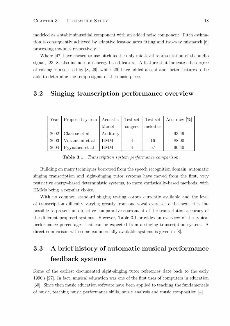
3.2 Singing transcription performance overview
Year Proposed system Acoustic Test set Test set Accuracy [%]
Model singers melodies
2002 Clarisse et al Auditory - - 93.49
2003 Viitaniemi et al HMM 4 16 88.00
2004 Ryynanen et al HMM 4 57 90.40
Table 3.1: Transcription system performance comparison.
Building on many techniques borrowed from the speech recognition domain, automatic
singing transcription and sight-singing tutor systems have moved from the first, very
restrictive energy-based deterministic systems, to more statistically-based methods, with
HMMs being a popular choice.
With no common standard singing testing corpus currently available and the level
of transcription difficulty varying greatly from one vocal exercise to the next, it is im-
possible to present an objective comparative assessment of the transcription accuracy of
the different proposed systems. However, Table 3.1 provides an overview of the typical
performance percentages that can be expected from a singing transcription system. A
direct comparison with some commercially available systems is given in [8].
3.3 A brief history of automatic musical performance
feedback systems
Some of the earliest documented sight-singing tutor references date back to the early
1990’s [27]. In fact, musical education was one of the first uses of computers in education
[30]. Since then music education software have been applied to teaching the fundamentals
of music, teaching music performance skills, music analysis and music composition [4].

Chapter 3 — Literature Study 19
A prime example of music education technology is the Computer Assisted Instruction
(CAI) GUIDO system, developed in 1981 and used for practicing and testing aural skills
[17]. It used what is known as an “branching teaching program” [30], which essentially
matched the user’s performance to a preset reference and based on the deviation of the
user’s performance to that reference gave a preset advice as a response. For the teaching
of musical performance skills, the Piano Tutor Project was launched in 1989 [10]. Tutorial
feedback on novice piano performances is given, combined with pre-stored expert perfor-
mances of the same piece. Score-following techniques are used as a basis for detecting
student errors.
Simple and logical music activities, such as teaching the fundamentals of music, can
adequately be approached with a static predefined teaching program, with pre-stored
templates. But for activities involving music composition and performance, the dominant
technique is based on cognitive theories of learning. In view of this interactive educational
approaches seem to be more productive than practice drills and preprogrammed learning
tool. As the authors of the study [4] noted: “The development and improvement of music
performance skills relies on tools with aural and visual feedback as central elements”.
In 1998 Camboropoulos [5] set out to create a general computational theory for musical
structure, which seeks to obtain a structural description of a musical piece, regardless of
it’s context. But as noted in [4], there still seems to be a lack of a complete cognitive
musical theory to support musical teaching activities properly.
In a more recent study [48], the use of a real-time visual feedback system providing
information such as the input waveform, fundamental frequency, short-term spectrum,
narrow band spectrum, spectral ratio and the vocal tract shape, is shown to be quite
successful within a singing lesson context. According to the authors the recorded lesson
data, such as the digital audio-visual recordings had been helpful to the users. The
emphasis of the study is on the analysis of the student-teacher communication that takes
place during a typical lesson as well as the evaluation of the feedback system in the opinion
of singing teachers, and not on the development of the system itself. The study provides
a good oversight of the learning process and highlights some difficulties with regards to
the impartation of knowledge from teacher to student through conventional instructive
conversation.
A different study focused specifically on the feasibility of real-time audio-visual feed-
back with regards to pitch-accuracy training. Using 56 participants and two different
feedback systems shown in Figure 3.5, the resulting pitch tracks were segmented by hand
and measured against reference transcriptions to compute the average pitch error made.
In this way the average improvement for the different groups with and without real-time
audio-visual feedback aid can be compared. It was concluded that for the group of un-
trained as well as the group of trained singers, a notable improvement can be observed

Chapter 3 — Literature Study 20
(a) (b)
Figure 3.5: Graphical user interfaces of the two real-time audio-visual feedback systems
used in [49].
after a period of time when using feedback aid [49].
3.4 Sight-singing tutor system considerations
It is useful to note that the problem of scoring user-input in sight-singing tutor systems
and the input-to-target melody matching problem in QBH systems do have a number of
similarities. In both cases the user’s audio will be matched, on some musical level, against
a target melody and a matching score computed. One of the main differences in approach
between the two applications is that a sight-singing tutor wants to reflect the differences
between the input and target melodies whereas data retrieval systems want to absorb as
much of these errors as possible. The implication of this difference is that QBH systems
have more freedom in the level of input representation and may manipulate or simplify
the input to fit the matching algorithm. In contrast to this, for singing-tutor systems the
singer’s input has to be represented as accurately as possible.
In [28] an HMM-based error model was designed especially to absorb various differ-
ent errors between a sung query and it’s target, in an effort to improve QBH system
performance by making the matching process more flexible and robust with regards to
inaccurate singing. The matching was performed on a simplified high-level pitch-duration
pair representation of the audio input, with both the pitch and the duration being quan-
tized to integer MIDI bins or duration bins.
In the majority of cases, sight-singing tutors give feedback using some of the important
features of singing, such as the pitch, spectrograms, and the vocal tract shape. However,
one of the problematic factors regarding this presentation level is that it is not central

Chapter 3 — Literature Study 21
to the singers’ frame of reference. Singers for example, may find spectrograms and pitch
tracks too far removed from their accustomed musical notation. It remains to be seen,
whether audio-visual feedback at a note level in the same form as the reference music
score, would not be a more satisfactory presentation format.
An intonation deviation study by E. Pollastri [34], separated sung notes into one
of four intonation pattern models. Although, these intonation classification models are
designed to aid a QBH system in the melody matching process, it could be beneficial for
tutoring systems to be aware of these intonation tendencies, especially that of vibrato. If it
is considered that a study by Prame et al [35] showed the common vibrato pitch deviation
range to vary between 34 and 123 cents, vibrato detection would be a very helpful aspect
to incorporate within a sight-singing tutor system.
Finally, in an exploratory study, Reiss et al [37] shows some alternative musical score
visualization techniques. These include, a spectrogram analogue, where timbre informa-
tion is discarded and the frequency information is interpreted and quantized as notes.
Different music parts are also shown in separate colours. In another representation dy-
namic contours of each instrument are plotted against time. This is a useful tool in
visualizing the overall structure of the musical piece. Using this representation it may be
easy to see recurring themes and the switching of the melody from one part to the other.
These are compared to standard music notation and some suggestions are made as to the
enhancement of the visual representation of music.
If indeed such diverse music representation schemes are found useful with regards to
singing education, these ideas may well be integrated into sight-singing tutor systems in
the future.
3.5 Conclusion
Although recent statistical modeling approaches have yielded recognition results of 90%
and above, these have yet to be tested on different datasets and under different conditions.
The accuracy of the time-alignment these systems produce has also not been explored.
Our overall aim is to develop a sight-singing tutor system which gives individual note-
based feedback. Since automatic singing transcription is a sub-problem of a sight-singing
tutor system, we will initially focus on the transcription problem itself. Our singing
transcription system will be based on statistical note models and these models will be
trained on real data. This will hopefully aid in the ability of the models to reflect actual
vocal behaviour.
Our intitial baseline HMM note models will be very similar to those proposed by
Ryynanen et al [29]. These will be incrementally expanded to incorporate ideas used
within the speech processing field to counter data sparsness, model context-dependency

Chapter 3 — Literature Study 22
and improve the time-alignment of notes.

Chapter 4
Corpus
4.1 Motivation
As it is in the field of automatic speech recognition, the statistical nature of HMMs require
that a substantial amount of recorded singing data is to be available for training to be able
to create representative musical models. Unfortunately, since little research is currently
being invested in the music processing field, no suitable existing singing corpus could be
found. It has therefore become one of the project aims to record and assemble a small
but useful dataset, for our application as well as for future research in this field.
In an effort to avoid unnecessary pitch interference, the recorded singing was unac-
companied and monophonic in nature. We have specifically chosen to limit the data to
the soprano voice. This allows for a restricted note range, which in turn results in fewer
notes to be modeled. In the light of the data scarcity such focusing of the data resources
is essential. Although voice ranges may differ in terms of their characteristics, we are of
the opinion that a system developed for one voice range should be expandable to other
ranges without major changes, once data for those ranges become available.
4.2 Material
Figure 4.1 shows a subsection of the Unisa technical exercises found in the grade III, IV
and V syllabus [45]. Each music score line in the figure is a separate exercise and most
of the exercises are single legato phrases consisting of approximately 10 notes. After each
exercise the student would rest for a few seconds and receive feedback from the teacher.
For most exercises a piano chord or arpeggio was given to help the student achieve the
correct pitch from the start.
In the interest of preserving a singer’s vocal chords, the set of muscles controlling
the vocal chords needs to be stretched gradually in much the same way as other muscles
groups in the body needs to be warmed-up prior to them being extensively used. For this
23

Chapter 4 — Corpus 24
Figure 4.1: Examples of Unisa technical exercises used in the compilation of the corpus.
reason, one of the purposes of vocal training exercises is to serve as a pre-performance
vocal warm-up for singers. Sensibly, slow legato phrases within a comfortable pitch range
are typically used for this purpose. Once the singer’s voice has become more flexible,
notes on the edge of the singers’ vocal range can gradually be reached. Rapid up-and-
down staccato jumps are also used to prepare the voice for the agility typically needed in
the performance of musical pieces.
Apart from loosening the vocal chord muscles, the exercises are designed to train
correct intonation within a phrase of notes, produce a brilliant tone and improve overall
pitch accuracy. The vocal range of a singer can also be improved in a systematic manner
by shifting the key incrementally until a student is challenged to produce the correct pitch
of the top or bottom notes consistently. By repeating the process, a student’s vocal range
can be monitored over a period of time for improvement.
4.3 Recording equipment and setup
The ProTools LE 7.1 recording software and a Rhode NT2000 Studio Condenser Micro-
phone were used for the preparation of our corpus. All recordings were stored using 16-bit
linear encoding at a sampling rate of 44.1kHz.
Each singer was recorded while taking a normal singing lesson, which begins with
technical exercises as warm-up for the voice of the student. Students were recorded in
the music rooms of Stellenbosch University’s Faculty of Music. The music session was
recorded as a single segment, making it easy later to group all the exercises of a particular

Chapter 4 — Corpus 25
UNISA
MUSIC ROOM
RECORDING ROOM
DSP LABORATORY
sessionwholeRecord
sessions intointo exercisesand annotate
SegmentSubject
Figure 4.2: Schematic of the recording steps.
student. The recording workstation and associated hardware were positioned in a separate
nearby room and linked to the microphone via a standard XLR1 microphone cable. The
audio was stored as 16-bit PCM audio files and the annotation as text files using the HTK
labelling format [1, pg. 81]. These steps are schematically depicted in Figure 4.2.
4.4 Annotation
The final dataset contains only sung notes and silences. Initially separate models were to
be used for notes of similar pitch but different diatonic2 context (for example A♯ and B♭).
This design choice was made to facilitate the correct transcription of notes in terms of
their context within the key structure. Successful implementation of this discrimination
would certainly aid in the key estimation process. However, with severely limited training
instances per note this was not feasible. Furthermore key estimation is not essential within
a sight-singing tutor system. It is also doubtful whether the diatonic note context would
lead to significantly different note model characteristics.
Most of the technical exercises are legato phrases. This makes segmentation based
on the energy envelope of the audio input signal, used by a number of QBH systems,
unhelpful and also limits the use of the voicing parameter (introduced in Section 5.1) as
a feature.
Notes are therefore uniquely defined at semitone level using a format similar to the
MIDI standard notation. An illustration of the annotation process for a single phrase
1eXternal Left Right or eXternal Live Return connector.
2The term “diatonic” generally refers to music derived from the modes and transpositions of the “white
note scale” C-D-E-F-G-A-B. In other words, music of (or using) only the seven tones of a standard scale
without chromatic alterations. In some contexts, especially the more modern usage of the term, it may
include all different heptatonic scale forms that are in common use in Western music [12].

Chapter 4 — Corpus 26
Figure 4.3: Screenshot of the annotation process using the Wavesurfer software
package [44].
using the Wavesurfer software package is shown in Figure 4.3. For example, middle C,
middle C♯ and D an octave above middle C are reduced to c4, c4s and d5 respectively.
Repetitive notes not separated by a silence are transcribed as a single note, hence it is
guaranteed that all notes are separated by either silence or a transition.
During the labelling process these segments are further separated into musical phrases.
The phrases may constitute a whole exercises or only part of one. The labeling process is
similar to that of speech, except that the labels cannot be determined just by listening to
the audio file. Each phrase is treated individually with the labeling software as shown in
Figure 4.3, listened to carefully (a tuned instrument such as a keyboard or piano assisted
the annotator in this regard) to determine the relevant key and structure. Each note is
then labeled and stored in the standard HTK label format.
One challenging aspect of using technical exercises instead of performed pieces of
music is the fact that the exercises are artificial musical phrases designed to challenge the
students and to exercise the voice in some extreme way. This sometimes results in a novel
sequence of notes that is not only hard for the student to master, but also challenging to
transcribe. A corpus dedicated to a specific musical genre would be expected to exhibit
certain common musical traits, especially within a specific musical piece. In contrast, one
technical exercise may differ vastly from the next as they are designed to be representative
of different styles, aspects and techniques of singing. Some technical exercises are designed
to help students “glide over” notes in an effort to create the desired musical contour. This
results in pitch track segments of shorter notes conforming closely to transition regions
between notes rather than stable notes. Such segments were difficult to annotate since
the boundaries of the notes are much less clear than when they are sung more distinctly.
Extreme cases, where notes were too hard to identify, were removed from the the corpus.

Chapter 4 — Corpus 27
4.5 Corpus statistics
The typical range of a soprano voice in terms of notes, is illustrated in Figure 4.4. The
combined range of all the soprano voices in the dataset is shown in Figure 4.5. Some of
our soprano voices tended to lean more towards mezzo-soprano, thereby extending the
lower limit to below middle C. Although the notes outside of the typical soprano range
are at the extremities of the capabilities of the students and therefore have very few
training examples, we have included them in the dataset to maximize the small amount
of data available. The challenge presented by these undertrained models will be one of
the concerns throughout the modeling process in the sections to follow.
Figure 4.4: Typical pitch range of a soprano voice. Middle C is indicated.
Figure 4.5: Pitch range encountered in our corpus. Middle C is indicated.
Figure 4.6 shows the number of times each note was encountered in our corpus. It can
be seen that the dataset occurrence density distribution resembles a Gaussian distribution.
As mentioned above this distribution has to do with the common range of the different
singers as well as the fact that ascending and descending scales together with arpeggios
and other exercises tend to have most notes within comfortable singing range and often
build up to a crescendo on a single outlying note.
Table 4.1 provides information regarding the overall size and range of the dataset, as
well as a view of the dataset training and testing partition ratios.
Decription Training set Testing set Total dataset
Number of exercise segments 1023 346 1369
Number of notes 10261 3581 13842
Number of singers 19 7 26
Range A3 − D6♯ A3 − D6♯ A3 − D6♯
Table 4.1: Corpus division ino training and test sets.
The general nature of the sequential note combinations encountered in our corpus is
shown in Figure 4.7. This figure shows the frequency with which a transition occurred

Chapter 4 — Corpus 28
a3 a3s b3 c4 c4s d4 d4s e4 f4 f4s g4 g4s a4 a4s b4 c5 c5s d5 d5s e5 f5 f5s g5 g5s a5 a5s b5 c6 c6s d6 d6s0
50
100
150
200
250
300
350
400
450
HMM NOTE MODEL NAME
NU
MB
ER
OF
NO
TE
OC
CU
REN
CES
Figure 4.6: Training set note occurrence distribution for the compiled corpus.
from each note to each other note. Most transitions span fewer than 5 semitones and
the most common transition found is the 2 semitone upward transition. This transition
magnitude is the most common one found in scales, contributing to 71% of major scale
transitions. The figures illustrate that when considering all possible note transitions, our
dataset remains extremely sparse.
10 20 30
5
10
15
20
25
30
10 20 30
5
10
15
20
25
300
20
40
60
80
100
120
140
160
0
5
10
15
20
25
30
NOTE(t+1)
NO
TE(t
)
NOTE(t+1)
NO
TE(t
)
Figure 4.7: Training set note transition distribution. The figure on the right is a scaled
version of the one on the left.

Chapter 4 — Corpus 29
4.6 Conclusion
An unaccompanied monophonic corpus comprising passages sung by a total of 26 soprano
students has been assembled. The data is acquired by recording routine lessons of the stu-
dents, with minimal invasion. Lessons are then segmented into modular musical phrases,
which are each hand labeled with the appropriate notes. Seeing that very few (if any)
singing corpora are currently available for research purposes, this training set can in itself
be considered one of the notable contributions of this project to the field.

Chapter 5
Feature extraction
Unlike speech recognition features that are focused mainly on pronunciation and are
largely pitch independent, singing transcription must focus on the pitch and be pronun-
ciation independent. Our system uses pitch, with delta-pitch added to assist in note
boundary detection. Given that the technical exercises of the dataset consist mainly of
single legato phrases, the energy envelope itself is not helpful for the extraction of note
event features. Many systems use adaptive pitch tuning [47, 29, 27], but since the system
will be expanded in the future to accommodate user feedback and would therefore need
an accurate account of the users’ pitch values, absolute pitch frequency is used instead.
5.1 The Yin pitch estimator
We use the Yin algorithm as proposed in [19] as our primary pitch estimator. This
algorithm has been found to be effective in other music transcription systems [47, 29].
Even though the algorithm is explained in detail by the authors in [19], the algorithm
benefits are discussed with regards to speech processing only. This section will briefly
highlight the algorithm steps and comment on the effectiveness thereof, with regards
specifically to singing transcription.
For a given discrete time-domain signal x, sampled at a frequency fs, the Yin algo-
rithm outputs the fundamental frequency fo at time t together with a voicing parameter
vt. Although the voicing parameter may be useful as far as segmentation of note bound-
aries is concerned, including it did not yield a general increase in transcription accuracy
in preliminary experiments. Therefore, in an effort to minimise the number of different
system combinations we have opted not to include results based on the systems incorpo-
rating this feature. The Yin pitch estimation method is closely related to the well known
auto-correlation function (ACF), but is improved by a series of steps that seek to minimize
the weaknesses of the ACF within the scope of implementation. The ACF evaluated at
time index t, which we denote as ft, is defined as:
30

Chapter 5 — Feature extraction 31
ft(τ) =
t+W∑
j=t+1
xjxj+τ (5.1)
Here τ is the autocorrelation lag, W is the summation window size and x the input
waveform. This ACF calculation is unbiased with regards to the lag variable τ and is
called the unbiased ACF. Alternatively the ACF can be defined to reduce the summation
range as the lag, τ increases:
f ′t(τ) =
t+W−τ∑
j=t+1
xjxj+τ (5.2)
This creates an ACF envelope that decrease as the lag period τ increases, which in
turn effectively penalizes higher order lag peaks and is hence termed the biased ACF. An
example demonstrating the differences in these equations is given in Figure 5.1. The period
of x is found by choosing the highest non-zero lag peak by examining the function at all
other possible lag periods. For a window size of more than double the input signal period
there will be peaks within the ACF at multiples of the input signal period. Erroneous
selection of these peaks instead of the actual fundamental frequency lag period, is an
inherent weakness of the ACF as used in Equation 5.1. However, when using Equation
5.2 the period peak may be situated at a lag period that is significantly suppressed, such
that a value close to the zero lag boundary is chosen instead.
0 100 200 300 400 500 600 700 800 900−2
0
2
0 100 200 300 400 500 600 700 800 900−500
0
500
1000
0 100 200 300 400 500 600 700 800 900−500
0
500
1000
TIME [samples]
AM
PLIT
UD
E
LAG [samples]
AM
PLIT
UD
E
LAG[samples]
AM
PLIT
UD
E
Figure 5.1: Example of a periodic waveform (top), the auto-correlation function(ACF)
using Equation 5.1 calculated from the periodic wavefrom (middle) and the ACF
calculated using Equation 5.2 (bottom).

Chapter 5 — Feature extraction 32
In the light of these shortcomings, let us compare the ACF to the average magni-
tude difference function (AMDF) [39]. Taking the squared difference function dt(τ) and
averaging over the window length of W samples is similar to the AMDF function [11]:
dt(τ) =t+W∑
j=t
(xj − xj+τ )2 (5.3)
Here τ is again an integer lag variable such that τ ∈ [0, W ). The fundamental difference
between that of the AMDF function and the ACF may be illustrated by expanding the
AMDF squared difference in terms of the ACF:
dt(τ) = ft(0) + ft+τ (0) − 2ft(τ) (5.4)
Here ft(τ) still denotes the ACF at time t with a lag of τ samples. Using a 360 sample
extract from a speech signal as an example (at the top of Figure 5.2) we will attempt to
show why the results of the AMDF and ACF function differ slightly in some cases.
50 100 150 200 250 300 350−0.6−0.4−0.2
00.20.4
20 40 60 80 100 120 140 160 1805.65
5.75.75
5.8
20 40 60 80 100 120 140 160 180
2
3
4
20 40 60 80 100 120 140 160
−6−4−2
024
TIME [samples]
AM
PLIT
UD
E
LAG [samples]
AM
PLIT
UD
E
LAG [samples]
AM
PLIT
UD
E
LAG [samples]
AM
PLIT
UD
E
Figure 5.2: Speech waveform example (top), signal power term, ft(0) (second from the
top), energy term ft+τ (0) (second from bottom) and the scaled inverse of the ACF
function, −2ft(τ) (bottom).
The first term in Equation 5.4, ft(0), shown second from the top in Figure 5.2, relates
to the power withing the signal and is independent of the lag period as can be seen from
the example. The third term, −2ft(τ) , is just a scaled inverse of the ACF function
itself. The middle term ft+τ (0) however, describes how the signal energy profile varies

Chapter 5 — Feature extraction 33
with τ and is shown second from the bottom in Figure 5.2. It is essentially this additional
energy term which may result in a difference in the locations of the local ACF maxima
and AMDF minima. According to Hess and Kawahara et al [16, 19], one reason why
the AMDF algorithm may be prefered over the ACF can be seen in Equation 5.1. The
summation process in Equation 5.1 does not compensate for the effects of an increase or
a decrease in signal energy when calculating ft(τ). This effect can be observed in the
example given by examining the relationship between the summation of the AMDF and
ACF with respect to the lag period and the lag dependent energy term ft+τ (0) in Figures
5.2 and 5.3. A rapid energy change within the input waveform does result in a small but
noticeable difference between the two AMDF functions, shown in the bottom graph of
Figure 5.3. The effects of this ACF energy dependency is elaborated on further in [16].
However, it is only important to be aware of the existence of this subtle difference between
the algorithms, which has prompted the Yin algorithm to be AMDF based rather than
ACF based.
20 40 60 80 100 120 140 160 1800
5
10
20 40 60 80 100 120 140 160 180
−2
0
2
4
20 40 60 80 100 120 140 160
5.5
6
6.5
7
LAG [samples]
AM
PLIT
UD
E
LAG [samples]
AM
PLIT
UD
E
LAG [samples]
AM
PLIT
UD
E
Figure 5.3: AMDF, dt(τ) (top), ACF, ft(τ) (middle) and the difference of the two
functions dt(τ) − ft(τ) (bottom).
With no lag in the signal the difference function will be zero (i.e. dt(0) = 0). Speech
and singing will however not result in the difference function reaching zero at the funda-
mental period, because the periodicity will not be perfect. To avoid setting a lower limit
on the AMDF function, the “cumulative mean normalized difference function” proposed
in [19] is used instead:
The difference function is normalized by dividing it by the cumulative mean of the
function over shorter lag periods:
d′
t(τ) =
{
1 τ = 0
dt(τ)/[( 1τ)∑τ
j=1 dt(j)] otherwise

Chapter 5 — Feature extraction 34
This eliminates the need to define a lower limit for τ within d′
t(τ), since the “cumulative
mean normalized difference function” seeks to maximize the difference function for small
lag periods below the pitch period range of interest. This is important since defining
a set frequency threshold is not an ideal solution. Figure 5.4 compares the cumulative
mean difference function to that of the AMDF. The cumulative mean function is centered
around 1 and also approaches zero at multiples of the fundamental period. By normalizing
the difference function, it is possible to set an absolute threshold and choose the smallest
lag period that falls below this threshold.
20 40 60 80 100 120 140 160 180
0
2
4
6
8
10
20 40 60 80 100 120 140 160 180
0.5
1
1.5
2
LAG [samples]
AM
PLIT
UD
E
LAG [samples]
AM
PLIT
UD
E
Figure 5.4: The AMDF (top) and the cumulative mean differerence function (bottom).
In [19] it is briefly shown how dt(τ)/[( 1τ)∑τ
j=1 dt(j)] is proportional to the aperiodic
to total power ratio of the signal, although the threshold may be hard to fix to a specific
value. We have defined fundamental period candidates within the cumulative normalized
mean function where
dt(τ − 1) > dt(τ) < dt(τ + 1) (5.5)
We have used two criteria to determine the validity of a possible minima. Firstly, we
have implemented the power ratio threshold as mentioned above and secondly we have
defined a “minima sharpness” threshold which seeks to determine how prominent the
candidate peak is relative to the average sample of the window surrounding the peak.
The ratio of the function value at the minima candidate to the median of the surrounding
samples within a certain window is compared with a dynamic threshold to allow a maxi-
mum number of candidates. We have used a window size of 20 samples for this criterion
and have reduced the maximum number of candidates allowed to 4. Because the initial

Chapter 5 — Feature extraction 35
minima selection criteria is very inclusive, this process has been implemented to reduce
the candidate set to clear instances of periodicity.
However, since the input waveform contains predominantly uninterrupted singing, the
“cumulative normalized mean function” candidate minima were mostly unambiguous and
changes to the proposed criteria did not result in frequent changes in fundamental period
selection. The smallest lag period is selected from the set of valid minima as the funda-
mental period τ′. For improved frequency resolution or quantization error minimization,
the cumulative normalized mean function is interpolated over the interval {τ′−1, τ
′+1}.
The minimum of the interpolation polynomial is chosen as τp. The pitch period can then
be converted to an absolute frequency using fo = fs/τp. The voicing parameter vt is
given by d′
t(τp), which is the magnitude of the Yin function at τp. This parameter is a
function of the strength of the correlation at τp, which is related to the overall degree of
periodicity in the signal within the current frame. To enhance pitch continuity and reject
clear spurious peaks, only pitch values within the range of 27.5 – 2093.0 Hz (A0 – C7) are
accepted as valid, with invalid values set to the previous valid pitch value. Furthermore
the pitch track is smoothed with a 10th order median filter. This eliminates some of the
unresolved spurious octave errors.
100 200 300 400 500 600 700 800
400
500
600
100 200 300 400 500 600 700 800
−20
0
20
0 100 200 300 400 500 600 700 8000
0.5
1
SAMPLE NUMBER
SAMPLE NUMBER
SAMPLE NUMBER
FR
EQ
UEN
CY
[HZ]
DELTA
FR
EQ
UEN
CY
[HZ]
NO
RM
MA
GN
ITU
DE
PITCH
DELTA PITCH
VOICING
Figure 5.5: Typical pitch, delta-pitch and voicing features.

Chapter 5 — Feature extraction 36
5.2 Delta coefficients
The time differentials of the pitch values, referred to as delta coefficients, are calculated
at time t using the regression formula [1, p.63] given by:
dfo(t) =
∑Θθ=1 θ(fot+θ
− fot−θ)
2∑Θ
θ=1 θ2(5.6)
The window width parameter, Θ, is set to 2 in our experiments. Figure 5.5 illustrates a
typical pitch track and its associated delta-pitch and voicing values. For most note transi-
tions, the magnitude of the pitch gradient will be larger within the transition region than
it would be within the note regions. This makes the delta-pitch feature especially helpful
in the detection of note boundaries. By including the delta-pitch feature, the discrim-
ination between notes and transitions may be improved which would lead to improved
recognition accuracy and time-alignment.
5.3 Conclusion
In view of fact that the algorithm is already known within the singing transcription field
and has been applied successfully by others, for our application, the AMDF-based Yin
pitch estimation algorithm has been chosen as the main feature for the HMM acoustic
models. Some of the differences between the Yin function and that of the ACF and AMDF
have been discussed, and the advantages of the Yin function over these alternatives are
mentioned. Additional heuristics are also described, and examples of vocal exercise pitch
tracks, delta-pitch features and the voicing features are presented.
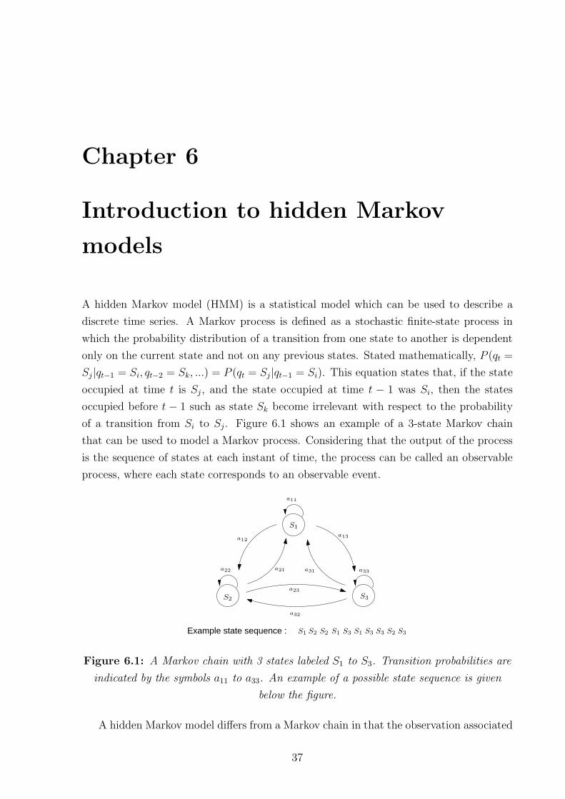
Chapter 6
Introduction to hidden Markov
models
A hidden Markov model (HMM) is a statistical model which can be used to describe a
discrete time series. A Markov process is defined as a stochastic finite-state process in
which the probability distribution of a transition from one state to another is dependent
only on the current state and not on any previous states. Stated mathematically, P (qt =
Sj |qt−1 = Si, qt−2 = Sk, ...) = P (qt = Sj|qt−1 = Si). This equation states that, if the state
occupied at time t is Sj , and the state occupied at time t − 1 was Si, then the states
occupied before t − 1 such as state Sk become irrelevant with respect to the probability
of a transition from Si to Sj. Figure 6.1 shows an example of a 3-state Markov chain
that can be used to model a Markov process. Considering that the output of the process
is the sequence of states at each instant of time, the process can be called an observable
process, where each state corresponds to an observable event.
Example state sequence :
a12
a21 a31
a13
a23
a32
a22
a11
a33
S1 S2 S2 S1 S3 S1 S3 S3 S2 S3
S1
S2 S3
Figure 6.1: A Markov chain with 3 states labeled S1 to S3. Transition probabilities are
indicated by the symbols a11 to a33. An example of a possible state sequence is given
below the figure.
A hidden Markov model differs from a Markov chain in that the observation associated
37

Chapter 6 — Introduction to hidden Markov models 38
with an HMM state is a probabilistic function of the state and not an observable event in
itself. The desired state sequence must now be inferred from an observation sequence O.
0 5 10
0.05
0.1
0.15
0.2
0.25
100 200 300 400
0.05
0.1
0.15
0.2
0.25
0.3
0.35
0.4
0 1000 20001
1.5
2
2.5x 10
−3
Example observation sequence :
a12
a21 a31
a13
a23
a32
a22
a11
a33
O1 O2 O3O4 O5O6O7
S1
S2 S3
P (vk|qt = S1)
P (vk|qt = S2)
P (vk|qt = S3)
vk
vk
vk
Figure 6.2: A Hidden Markov Model example with 3 states labeled S1 to S3. Transition
probabilities are indicated by the symbols a11 to a33.
An example of this concept is shown in Figure 6.2 and will be discussed in more detail
in the paragraphs to follow. Seeing that an audio signal can be considered a discrete
time series with variable length, and that a hidden quantity (the notes) must be inferred
from an observable quantity (the audio signal), singing input certainly qualify as feasible
input for HMMs. The ability of HMMs to model time varying stochastic processes is of
particular concern when applied to note modeling, since notes are sung differently from
one note to the next and from one singer to the next. Notes also differ in terms of length,
which requires stochastic duration modeling. This could also be considered an inherent
HMM capability as explained in [36, p.259].
The theory of Markov process modeling was originally published by Andrey Andreye-
vich Markov as early as 1906. Basic HMM theory was published somewhat later, between
1960 and 1970, by L. E. Baum et al [36, p.258]. Since the 1970s, HMMs have been a
popular means for modeling speech. The next section briefly highlights the basic theory
behind HMMs. For further reading, a comprehensive tutorial by L.R. Rabiner [36] on
HMMs is considered by many as the benchmark introduction to HMMs.
A Markov model as finite state machine consists of a finite number of states. Only
one state of an HMM is occupied at any given time, and moves from one state to the next
occur at discrete time intervals. The cost of moving to the next state or remaining in the
current state is determined by transition probabilities. The transition probability from
the current state i to the next state j is usually written as aij = P (qt = Sj|qt−1 = Si).
The inherent Markov property underlying HMMs allows all the transition probabilities
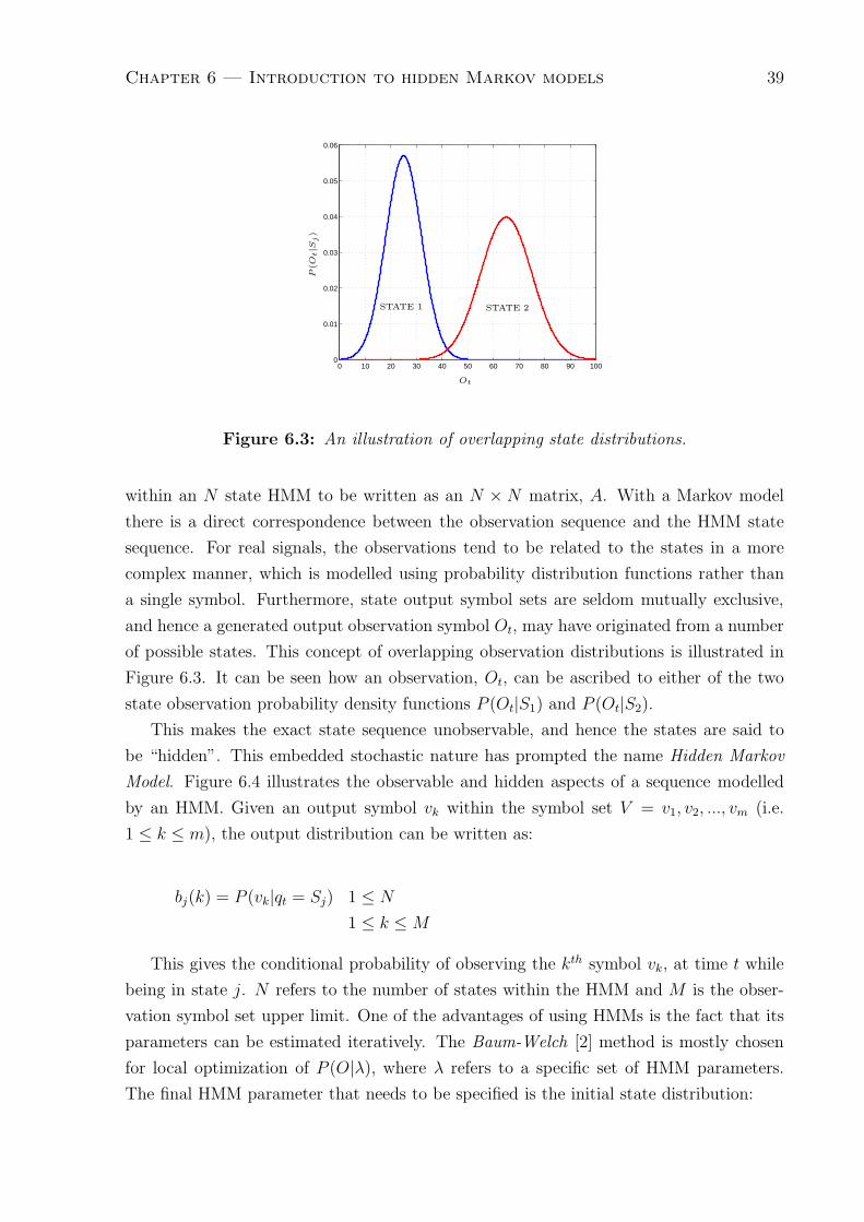
Chapter 6 — Introduction to hidden Markov models 39
0 10 20 30 40 50 60 70 80 90 1000
0.01
0.02
0.03
0.04
0.05
0.06
Ot
P(O
t|S
j)
STATE 1 STATE 2
Figure 6.3: An illustration of overlapping state distributions.
within an N state HMM to be written as an N × N matrix, A. With a Markov model
there is a direct correspondence between the observation sequence and the HMM state
sequence. For real signals, the observations tend to be related to the states in a more
complex manner, which is modelled using probability distribution functions rather than
a single symbol. Furthermore, state output symbol sets are seldom mutually exclusive,
and hence a generated output observation symbol Ot, may have originated from a number
of possible states. This concept of overlapping observation distributions is illustrated in
Figure 6.3. It can be seen how an observation, Ot, can be ascribed to either of the two
state observation probability density functions P (Ot|S1) and P (Ot|S2).
This makes the exact state sequence unobservable, and hence the states are said to
be “hidden”. This embedded stochastic nature has prompted the name Hidden Markov
Model. Figure 6.4 illustrates the observable and hidden aspects of a sequence modelled
by an HMM. Given an output symbol vk within the symbol set V = v1, v2, ..., vm (i.e.
1 ≤ k ≤ m), the output distribution can be written as:
bj(k) = P (vk|qt = Sj) 1 ≤ N
1 ≤ k ≤ M
This gives the conditional probability of observing the kth symbol vk, at time t while
being in state j. N refers to the number of states within the HMM and M is the obser-
vation symbol set upper limit. One of the advantages of using HMMs is the fact that its
parameters can be estimated iteratively. The Baum-Welch [2] method is mostly chosen
for local optimization of P (O|λ), where λ refers to a specific set of HMM parameters.
The final HMM parameter that needs to be specified is the initial state distribution:

Chapter 6 — Introduction to hidden Markov models 40
time
4
3
2
1
OB
SE
RV
AB
LEH
IDD
EN
OUTPUT
PDFs
Figure 6.4: A 4-state HMM example highlighting the observable and hidden aspects of
HMMs. Although the state sequence S1S2S2S3S4 gave rise to the observation sequence
o1o2o3o4o5, it is not possible to unambiguously retrieve the state sequence knowing only
the observation sequence.
πj = P (q1 = Sj) 1 ≤ j ≤ N
By denoting the set of N observation distributions by B, where N again refers to
the number of HMM states, each HMM can now be fully and compactly be defined by
λ = (A, B, π).
Since the re-estimation of model parameters are locally optimized, careful parameter
initialization would certainly aid in achieving predictable model convergence. Existing
techniques for obtaining a sensible estimate of the final state distribution include ini-
tialization of model parameters to the average of the training set features. This model
initialization to global parameters is known as a “flat start”. One advantage of this form
of initialization is that it does not require labeled training data.
Alternatively, by relying on training data uniformity, models may be initialized by
using the hand labeled training data boundaries for the initial training iteration, or by
uniformly segmenting the training files for the initial training iteration. Essentially these
techniques are designed to produce initial estimates, such that the estimates are closer to
the global probability distribution peak than any other local optimum probability. In the
case of optimizing pitch estimates, a typical note histogram as illustrated in Figure 6.5

Chapter 6 — Introduction to hidden Markov models 41
14 13 12 11 10 9 8 7 6 5 4 3 2 0 1 2 3 4 5 6 7 8 9 10 11 12 13 140
500
1000
1500
2000
2500
3000
3500
4000
4500
NOTE FREQUENCY BIN DISTANCE [SEMITONES]
NU
MB
ER
OF
SA
MPLES
Figure 6.5: Training set pitch estimation histogram of note A4#.
may be expected. Small peaks in the distribution due to octave errors, can be seen at 12
semitones below and 12 semitones above the target note frequency.
Thus for the pitch feature initialization, π is very likely to converge easily to the global
maximum, unless perhaps when π is initialized at around 12 semitones above or below
the target note frequency.
Like any other data driven or stochastic model the amount of training material needed
to obtain accurate model estimates can sometimes limit the use and success of HMMs.
In the chapters to follow, various data sparseness combating techniques are employed, to
reduce the effects of a small dataset, whilst still extracting as much benefit as possible
from the HMMs.
An HMM model will be used for each of the semitone notes (A3 − D6♯) within the
dataset. We will investigate different HMM topologies and state observation probability
density functions. In general we will estimate HMM parameters from the training set and
then evaluate the accuracy with which the test set can be transcribed.
6.1 Conclusion
The appropriateness of hidden Markov models as a statistical framework for singing, stems
from its ability to accurately segment a discrete time series, when provided with enough
training data. The opportunity to borrow applicable HMM-based techniques from the
neighbouring speech processing field is also a strong motivational factor for this modeling
choice. Although brief, this introduction should familiarize the reader with some of the
most important aspects of HMMs to be used in the chapters that follow.

Chapter 7
Context-independent note models
“All things being equal, the simplest solution tends to be the best one.” -
Paraphrasing of Occam’s razor
In this chapter we will explore different context-independent modeling topologies for mu-
sical notes. By assuming context-independence, each note in a sequence is modelled
individually and independent of the notes around it. Hence the musical context is not
taken into account. This approach allows the model set to be fairly small and the overall
system complexity to be low. On the other hand, model simplicity tends to lead to a
reduction in modeling flexibility and may be less effective in utilising all aspects of the
training data. By choosing the simplest topology first and then adapting as needed, we
will present first an introduction to our experimental approach and then expand these ba-
sic concepts incrementally through a series of critical evaluation and testing procedures.
Based on observed shortcomings of the initial systems, the models will be gradually im-
proved in an effort to increase the overall transcription accuracy of the system and also
the quality of the time-alignment of the models.
7.1 Single-state system
One of simplest ways to model a note sequence using HMMs is by using a single state
for each note. Using twelve-tone equal temperament, we will begin by modeling each
semitone by a single-state HMM. A schematic representation of the system is presented
in Figure 7.1.
We evaluate this type of system, firstly using only pitch as feature, and then adding
the delta-pitch as a second feature dimension. For this system and all systems without
transition models to follow, we have initially used a simple grammar which can be written
in EBNF (Extended Backus-Naur Form). A schematic representation of the grammar can
be seen in Figure 7.2(a). Although very compact in definition, this grammar specifica-
tion does not prohibit repetitions of the same note. Indeed we have found this inclusive
42

Chapter 7 — Context-independent note models 43
F4 G4SILENCE
NULL NULL
Musical passage
Figure 7.1: A simple musical passage modelled by single-state context-independent
HMMs.
ENDSILENCESILENCE
BEGIN
NULLNULL
NOTE
NOTE
A
B
(a) Simple grammar
ENDSILENCESILENCE
BEGIN
NULLNULL
NOTE
NOTE
A
B
(b) Non-repetitive grammar
Figure 7.2: Context-independent grammar schematic representations when no
transition modeling is applied.
grammar specification to result in multiple repetition errors. Although note repetitions
do occur within music pieces in general and indeed within the singing phrases in our
dataset, they are very difficult to detect since there is no transition region and with-
out any pronunciation restrictions, the signal envelope alone is not sufficient for reliable
segmentation.
Thus we have chosen to merge repetitions of the same note in the transcription refer-
ences and proceeded to modify this grammar specification so that a note may be followed
by a silence or any other note other than itself. Figures 7.2(a) and 7.2(b) offer a graphical
schematic representation of both grammars. Unfortunately, we have not found a compact
EBNF solution for the non-repetitive grammar specification and proceeded to create the
network lattice directly from the visual representation presented in Figure 7.2(b). We
have proceeded to use the non-repetitive grammar for all the experiments in Sections 7.1
to 7.5.
The system performance for both feature vector sets is shown in Table 7.1. The system
has a modest 54.58% note performance accuracy. The accuracy calculation is defined as

Chapter 7 — Context-independent note models 44
Features Used Note Accuracy [%] Substitutions Insertions Deletions
P 54.58 810 356 449
P+D 31.92 981 650 790
Table 7.1: Single-state context-independent system performance.
follows:
Accuracy =N − D − S − I
N× 100%
Where N is the total number of notes in the transcription reference, D the number
of deletion errors, I the number of insertion errors and S the number of substitution
errors. The default HTK error weights [1] have been used to evaluate our system. A more
detailed view of the system recognition is provided in Figure 7.3 by means of a confusion
matrix.
The diagonal represents the number of correct note recognitions, whereas the remain-
der of the matrix space shows the semitone interval placement of substitution errors. Due
to the fact that the ratio of training data to HMM states for a single-state system is at
a maximum relative to the more complex architectures we will consider in subsequent
sections, the HMMs are comparatively well trained. However, for a number of the note
models (eg. note model 15), the maximum is not located on the matrix diagonal. These
are note models which have a significantly higher pitch standard deviation than the other
models. For example note model 15 (C5) has a standard deviation of 417.20Hz, which is
52 times greater than the neighbouring note model pitch standard deviation. This situa-
tion makes it possible for the probability of the model’s own mean to be is overshadowed
by one or both of the neighbouring probability distributions which have much smaller
variances. For the note models closer to the edges of the training set the differences in
variance can be due to undertraining.
However, for most notes, the broadening of the variances is due to a lack of pitch
modeling flexibility within the single-state modeling topology which in turn results in an
inability to negotiate octave and fifth pitch track errors. Another drawback of the single-
state system is the lack of robustness and flexibility in modeling note duration. This is
reflected by a drop in system performance to a note accuracy of 31.92% when delta-pitch
is added as a second feature dimension. Since the delta-pitch feature indicates regions of
stability as well as transitions between notes, it conveys mostly note duration information
which cannot be modelled adequately by a single state. Indeed, Table 7.1 shows the
reduced performance to be mainly due to insertion and deletion errors. This reflects a
lack of transition and duration modeling capacity due to the single-state restriction.

Chapter 7 — Context-independent note models 45
Confusion Matrix − Pitch Only − 1 State HMM System
5 10 15 20 25 30
5
10
15
20
25
30 0
10
20
30
40
50
REFERENCE HMM MODEL NUMBER
REC
OG
NIZ
ED
HM
MM
OD
EL
NU
MB
ER
Figure 7.3: Confusion matrix for the single-state system using pitch as a feature.
Because the different stages of a note are not modeled separately, but are combined
into a single state, the system is less likely to be able to detect note boundaries correctly,
especially when the pitch track does not resemble a well defined note. A related drawback
is the associated poor convergence of the state means during training. Great care has to
be taken with the initialization of the state means, since convergence to an incorrect local
maximum of P (O|λ) due to variations in the pitch estimate, would result in an even
greater number of errors. An example is illustrated in Figure 7.4 where the mean of note
B5 has converged to the incorrect frequency, that of the note model F5, several semitones
lower.
a3a3sb3 c4c4sd4d4se4 f4 f4sg4g4sa4a4sb4 c5c5sd5d5se5 f5 f5sg5g5sa5a5sb5 c6c6sA3
B3
C4#
D4#
F4
G4
A4
B4
C5#
D5#
F5
G5
A5
B5
C6#
Fre
quency
Note model
Figure 7.4: Means of the single-state context-independent system after training.
In this case the convergence is neither to a nearby nor to a harmonically-related fre-
quency. By looking at the feature vector distributions given in the form of histograms in

Chapter 7 — Context-independent note models 46
1200 1300 1400 1500 1600 1700 18000
50
100 a5#
1200 1300 1400 1500 1600 1700 18000
50
100b5
b4 f5
1200 1300 1400 1500 1600 1700 18000
50
100 c6
FREQUENCY BIN NUMBERO
CC
UR
EN
CES
FREQUENCY BIN NUMBER
OC
CU
REN
CES
FREQUENCY BIN NUMBER
OC
CU
REN
CES
Figure 7.5: Pitch estimate histograms for the notes A5# (top), B5 (middle) and C6
(bottom).
Figure 7.5 and by comparing the neighboring note model histograms, it is apparent that
note B5 exhibits a substantial number of octave errors. However, in this case the obser-
vation probability given this note model, P (O|λB5), is maximized when the distribution
mean is between the two local distribution maxima, resulting in a large variance for the
single mixture. This is substantiated by Figure 7.6, which shows the note model mean
and variance at different training iterations. It is interesting to note how the mean first
shifts towards the desired value for B5, then moves towards the local maximum located
at B4, and eventually to an intermediate value between these two frequencies. Figure 7.7
shows the convergence of a note model for which there are a relatively low percentage
of octave pitch estimation errors. Here the variance decreases as the number of training
iterations increase, as expected. Convergence also requires fewer training iterations.
The shortcomings of the single-state system can be addressed in several different ways.
A greater number of Gaussian mixtures per state would add to the flexibility in the
frequency domain, whereas an increased number of HMM states per model would improve
duration modeling as well as absorb pitch estimate errors. We continue by first pursuing
the latter solution.

Chapter 7 — Context-independent note models 47
0 2 4 6 8 10 12 14400
500
600
700
800
900b5
f5
0 2 4 6 8 10 12 142
4
6
8x 10
4
NUMBER OF TRAINING ITERATIONS
FR
EQ
UEN
CY
[Hz]
NUMBER OF TRAINING ITERATIONS
SQ
UA
RED
FR
EQ
UEN
CY
[Hz2]
Figure 7.6: Convergence of the Gaussian mixture mean (top) and variance (bottom)
for the single-state HMM note model B5.
2 4 6 8 10 12 14 16200
400
600
800
a4#
2 4 6 8 10 12 14 160
1
2
3
4x 10
4NUMBER OF TRAINING ITERATIONS
FR
EQ
UEN
CY
[Hz]
NUMBER OF TRAINING ITERATIONS
SQ
UA
RED
FR
EQ
UEN
CY
[Hz2]
Figure 7.7: Convergence of the Gaussian mixture mean (top) and variance (bottom)
for the single-state HMM note model A4#.

Chapter 7 — Context-independent note models 48
F4
Musical passage
NULLNULL
SILENCE G4
Figure 7.8: A single musical passage modelled by multi-state context-independent
HMMs.
7.2 Multi-state system
A left-to-right non-skipping HMM topology as depicted in Figure 7.8 has been used to
increase the number of HMM states used to model each note. By restricting transitions
from any state i in the HMM to the next state i + 1 or back to the current state i,
a sequential progression through all states is guaranteed and adequate training of all
HMM states thereby encouraged. The choice of a non-skipping topology is based on
the assumption that all note events can be broken up into consecutive stages, such as a
common onset, stable part and a final region, sometimes also referred to as the “silence”
region [29]. The number of states used in our experiments ranges from 2 to 6. The aim
of increasing the number of states within each model is to allow the different sequential
stages of a note event to be modeled more explicitly.
For a two-state HMM system, Figure 7.9 shows the means and variances for the set
of note HMMs. It is apparent that in this case the first state appears to model the stable
note regions, while the second state tends to model the transition to the succeeding note.
In order to allow unambiguous segmentation into stable note and transition regions, for
HMMs with 3 or more states one would generally like to see the initial state of the model
depicting the preceding transition region as well as the note onset region, the middle state
focused on the stable core of the note event and the last states should model the trailing
transition region or note ending.
However, there is no guarantee that the states would automatically assume this order
during training, as can be seen in Figure 7.10. In practice the general convergences of
HMM states do not tend to reliably reflect this correspondence to stages of a note. One
of the reasons for this is that transition regions are in fact shared by their surrounding
notes, leading to variability of the alignments between the HMM states and the stages
of the note. Some transition regions may fit the outside states of particular note models
well, reducing the ability of the note models to represent the diversity of all the different
transition possibilities. Figure 7.11 illustrates a pitch track for 3 notes, together with two
possible HMM state alignments.

Chapter 7 — Context-independent note models 49
Figure 7.9: Gaussian means and variances for a two-state context-independent HMM
system after training.
Figure 7.10: Gaussian means and variances for a three-state context-independent
HMM system after training.

Chapter 7 — Context-independent note models 50
HMM State
Number
HMM State
NumberF
requ
ency
[Hz]
1 2 3 1 2 3 1 2 3
1 2 3 1 2 3 1 2 3
NoteNumber 2 31
Alig
nmen
t 1
Typ
ical
Alig
nmen
t 2
Typ
ical
Time [10 ms units]
Pitch track
Figure 7.11: An illustration of how the state alignment may vary for a particular
sequence of notes.
From Figure 7.11 it can be seen that different models can have different state-to-note
event correspondence. This may result in poor system performance as far as some note
combinations are concerned, because certain model combinations may be misaligned in
such a way that neither of the models are capable of modeling the common transition
region. Another scenario would be neighboring notes which are both trained to model the
shared transition region. The most suitable model is selected to model the region, which
increases the cost of the rejected model.
Number of HMM States Accuracy[%] Substitutions Insertions Deletions
2 81.47 231 183 245
3 78.85 258 219 275
4 79.70 258 205 259
5 80.43 256 190 250
6 81.10 255 193 224
Table 7.2: Multi-state system performance when using only pitch as feature.
The performance of systems using between 2 and 6 HMM states per note are dis-
played in Tables 7.2 and 7.3. All of the systems show a substantial improvement over the
single-state system performance, with a general performance increase associated with an
increase in the number of HMM states. This may indeed be a further indication that any
aid with regards to duration modeling is of importance for the current system. Further-
more, with some form of sub-note modeling being applied the added delta-pitch feature
dimension leads to a consistent increase in performance. Because of the one-to-one corre-

Chapter 7 — Context-independent note models 51
Number of HMM States Accuracy[%] Substitutions Insertions Deletions
2 76.77 243 296 287
3 81.55 182 211 263
4 83.21 200 163 234
5 84.17 196 159 208
6 83.44 199 171 219
Table 7.3: Multi-state system performance when using pitch and delta-pitch as features.
spondence between pitch frequency and our note models, single Gaussian mixture models
were normally used. Some experiments were however conducted using a larger number of
Gaussian mixtures in Section 7.4, in an attempt to absorb insertions due to octave and
fifth errors.
7.3 Preset Gaussian parameters system
Unlike the speech recognition field where optimal parameter values are not known due
to the intrinsic variability of speech sounds, with musical note modeling the ideal pitch
mean of the stable part of the note is known beforehand. The trained means of the single-
state HMM system are shown in Figure 7.4 in Subsection 7.1 and it can be seen that in
most cases these correspond to the ideal frequencies. It is believed that, with plenty of
training data and error-free pitch estimates, these means would all be aligned to the exact
frequencies of the equally tempered scale.
Number of HMM States Accuracy[%] Substitutions Insertions Deletions
1 54.33 771 434 419
2 79.81 252 251 215
3 80.06 211 256 242
4 81.95 209 240 193
5 82.54 220 224 177
6 83.24 188 225 183
Table 7.4: Multi-state system performance when using preset Gaussian means and only
pitch as feature.
By similar reasoning, the pitch variances of the models may be set to theoretically
sensible values. To determine these, the HMM state means are first set to correspond to

Chapter 7 — Context-independent note models 52
Number of HMM States Accuracy[%] Substitutions Insertions Deletions
1 31.19 959 833 655
2 75.67 268 334 263
3 80.60 196 271 223
4 83.44 206 210 173
5 84.14 191 204 169
6 84.06 202 208 157
Table 7.5: Multi-state system performance when using preset Gaussian means and
using both pitch and delta-pitch as features.
1 2 3 4 5 6−2
−1
0
1
2
3
P
P+D
REC
.AC
CD
IFF[%
]
NUMBER OF HMM STATES
Figure 7.12: Performance improvement when using preset Gaussian means relative to
trained means when using pitch (P) and when using pitch and delta-pitch (P+D) as
features.
the ideal frequencies, leaving the variances to be trained normally. By comparing Tables
7.4 and 7.5 which show the recognition results for the system with preset means, to Tables
7.2 and 7.3, it can be observed that a small but steady performance increase of around
2% note accuracy is achieved in this way. However, this is only the case when the number
of HMM states is greater than 3, and the performance increase rises with the number of
states. From Figure 7.12 the same trend can be seen for all features. This trend can be
understood by considering the trade-off between the amount of training data per state
and the flexibility to model different stages of a note event. For a small number of HMM
states (N < 3) fixing the HMM state decreases the ability of the note models to model the
transition regions and note event stages and thus leads to a deterioration in performance.
For N > 3 however, the accuracy of the preset state means is welcomed, and severe
undertraining of certain states is minimized. To summarize, it can be concluded that
pre-setting the Gaussian state means can be used to avoid the undertraining when the
ratio of training data to HMM states is known to be low. Note that the values in Tables

Chapter 7 — Context-independent note models 53
7.4 and 7.5 have been obtained by fixing the pitch means, but leaving the pitch variances
and transition probabilities to be trained using Baum-Welsh re-estimation.
Our next set of experiments attempts to pre-set both the HMM state means and the
variances. In particular, we will preset all variances to a global average obtained from the
training data.
57 57.5 58 58.5 59 59.5 60 60.5 610
0.1
0.2
0.3
0.4
0.5
0.6
0.7
0.8
0.9
1
MIDI semitone number
No
rma
lize
pro
ba
bili
ty d
en
sity
215 220 225 230 235 240 245 250 255
0.1
0.2
0.3
0.4
0.5
0.6
0.7
0.8
0.9
1
Frequency [Hz]
No
rma
lize
d p
rob
ab
ility
de
nsi
tyMIDI DOMAIN ABSOLUTE FREQUENCY DOMAIN
σMIDI σHz
pm1 pm2pf1 pf2
Figure 7.13: Illustration of the use of a preset variance in terms of MIDI semitones as
well as corresponding pitch frequency. The variance in the MIDI and absolute frequency
domain is indicated as σMIDI and σHz respectively. These values are related according to
Equation 7.1. pm1 and pm2 are the distribution mean and variance respectively in the
MIDI domain and pf1 and pf2 the mean and variance in the absolute frequency domain.
10 20 30
60
65
70
75
80
85
90
10 20 30
400
600
800
1000
1200
1400
1600
standard deviation
NOTE MODEL NUMBER
FR
EQ
UEN
CY
[MID
ISEM
ITO
NES]
NOTE MODEL NUMBER
FR
EQ
UEN
CY
[Hz]
Figure 7.14: An illustration of how a constant offset of 5 semitones on the linear MIDI
scale (left) translates to a non-linear offset on the absolute frequency scale (right).
Using MIDI values is especially convenient when working with semitone ratios, because
a preset global variance can be computed as a semitone fraction. To compute the average
variance over a range of different note frequencies, each variance is transformed to the
linear MIDI scale so that an average note variance in terms of semitones can be computed.
Only the standard deviation of note models with over 200 note instances in the training set

Chapter 7 — Context-independent note models 54
have been used to calculate the average standard deviation. The average “well-trained”
note standard deviation was calculated to be 0.50022 MIDI semitones. We have chosen
the preset standard deviation to be 0.5 MIDI semitones as illustrated in Figure 7.13.
Using this preset standard deviation value, variances can be determined for each different
note model in the absolute frequency domain. This is a non-linear transformation as
illustrated in Figure 7.14. In order to transform the global standard deviation from its
specification in terms of MIDI semitones to an absolute frequency deviation vector the
Hz-to-MIDI transformation is inverted as follows:
σHz = e(M+σMIDI−69)×log 2/12 ∗ 440 − e(M−69)×log 2/12 ∗ 440 (7.1)
here σHz denotes the vector of standard deviations for the set of models in the absolute
frequency domain and M denotes the model set means in the MIDI domain. σMIDI is
the global standard deviation in the MIDI domain, chosen to be 0.5 semitones for our
experiment. An example of the standard deviations chosen in this way is given in Figure
7.15.
220 230 240 250 260 270
0.1
0.2
0.3
0.4
0.5
0.6
0.7
0.8
0.9
1
A3# B3
FREQUENCY [Hz]
NO
RM
ALIZ
ED
PR
OB
AB
ILIT
Y
σMIDI
Figure 7.15: An illustration of the use of a preset standard deviation (σMIDI), for
notes A3♯ and B3.
The performance of a system in which means take on their ideal values and vari-
ances are computed according to Equation 7.1 is shown in Table 7.6. The system has
been evaluated with regards to the pitch feature only. As can be expected, because the
probability density function parameters are highly constrained, the results vary within a
correspondingly narrow margin (75% to around 78%).
Compared to the previous system results in Tables 7.4 and 7.5, fixing the model
variances has led to a deterioration in the overall recognition accuracy of the system.

Chapter 7 — Context-independent note models 55
Number of HMM States Accuracy[%] Substitutions Insertions Deletions
1 75.00 154 168 241
2 77.04 166 165 186
3 77.09 168 179 169
4 78.11 164 133 196
5 78.20 166 116 209
6 78.20 161 112 218
Table 7.6: Multi-state system performance when using preset Gaussian means and
variances, and when using pitch and delta-pitch as features.
Even though it appears that the variance of the pitch values for each note have a standard
deviation of less than 0.5 semitones as illustrated by the spacing between the peaks in
Figure 7.16, it appears that flexibility in terms of the variance values is still needed to
model the transition regions accurately.
a3 a3s b3 c4 c4s d4 d4s e4 f4 f4s g4 g4s a4 a4s b4 c5 c5s d5 d5s e5 f5 f5s g5 g5s a5 a5s b5 c6 c6s d6
200
400
600
800
1000
1200
1400
1600
1800
MIDI FREQUENCY BINS
NU
MB
ER
OF
SA
MP
LE
S
Figure 7.16: Distribution of training set pitch estimates.
As mentioned in Section 7.1, the addition of HMM states may assist in modelling the
sequential stages of a note, which is related to different pitch variance profiles as pointed
out in [29]. The effectiveness of using fixed variances may be improved by taking these
note event stages into account, but this approach has not been pursued in this thesis.
Unlike the case when only the state means are pre-set, the performance deteriorates

Chapter 7 — Context-independent note models 56
for all different state configurations when both means and variances are pre-set (3.21%
average performance decline over 2 to 6 HMM states systems) with the exception of
the single-state system, for which the performance increase was 14.03%. Furthermore,
the system with additional pre-set variance parameters performs better during the first
training iteration when all state parameter are still very inaccurate.
7.4 Multiple Gaussian mixture system
Histograms of the pitch estimates for two example note models are presented in Figure
7.17. The data for the A4# note example (the graph on the left), appears to resemble a
single Gaussian distribution, with one clearly defined peak. However, the A3# model on
the right has two clearly defined peaks: one at the theoretical mean and another due to
pitch estimate errors. The suitability of the training data for multiple mixture modeling
varies for different notes, since the prevalence of such pitch errors is not the same for all
notes.
1000 1500 20000
200
400
600
800
1000
1200
1400
1600
1800
2000
800 1000 12000
10
20
30
40
50
60
70
80
90
100
MIDI BIN NUMBER
NU
MB
ER
OF
OC
CU
REN
CES
MIDI BIN NUMBER
NU
MB
ER
OF
OC
CU
REN
CES
Figure 7.17: Pitch feature histogram of A4# model(left) and A3# model(right).
One problem with multi-mixture modeling of the pitch feature is that the peaks of the
feature distribution are usually significantly separated by the frequency ratio, fharmonic,
where
fharmonic =f0
Nfor all N ∈ · · · ,
1
4,1
3,1
2, 2, 3, 4, · · · (7.2)
and where f0 is the fundamental pitch frequency. This is due to the high percentage
of octave or fifth interval pitch estimation errors. This significant amount of separation
between peaks located at the true pitch and at its harmonics can lead to poor convergence
of the mixture model’s parameters. For example, if the mixture means are not initialized
to lie close enough to the smaller peaks, all means may simply converge to the true mean,

Chapter 7 — Context-independent note models 57
leaving the system performance unchanged. Secondary mixtures should be initialized to
lie far enough from the true pitch peak, for example at octave intervals from it.
a3a3sb3 c4c4sd4d4se4 f4 f4sg4g4sa4a4sb4 c5c5sd5d5se5 f5 f5sg5g5sa5a5sb5 c6c6s
1
1.5
2
2.5
3
HMM MODEL NUMBER
FR
EQ
UEN
CY
RAT
IO
Figure 7.18: Ratio of 2nd to 1st Gaussian mixture mean after re-estimation.
It should be noted however, that since the distribution of harmonic pitch estimate
errors differs from note model to note model, such pre-setting heuristics cannot be guar-
anteed to be optimal for all models.
Nevertheless, we have conducted experiments using two HMM states, two Gaussian
mixtures per state, and initialising one set of mixture means to 2f0. These two-mixture
models have shown a small increase in performance (2.36% note accuracy). Figure 7.18
demonstrates that the 2nd mixture mean often converges to a frequency that is close to 2
times the mean of the first mixture, especially for the note models with a greater amount
of training data. The results of the experiments are given in Table 7.7. By comparing
these results with those in Table 7.1 and Table 7.2, a consistent improvement is evident.
The average improvement (excluding the 23.79% increase for the single-state system)
compared to the single-mixture system is 1.86%. We have also conducted multiple-modal
experiments using pitch and delta-pitch as features. However, the delta-pitch feature
distribution does not seem to exhibit the same multi-dimensional behaviour and the per-
formance during the experiments showed a decline in note-accuracy of over 25%.
Although the most common pitch estimate errors are a doubling of the true pitch, from
Equation 7.2 we see that erroneous estimates can occur at various multiples of the pitch
frequency. In the light of this we have also experimented with three Gaussian mixtures.

Chapter 7 — Context-independent note models 58
Number of HMM States Accuracy[%] Substitutions Insertions Deletions
1 78.37 232 304 233
2 83.69 192 194 194
3 81.61 240 232 182
4 81.27 260 134 272
5 81.61 241 202 211
6 82.68 260 111 245
Table 7.7: Multi-state two-mixture system performance when using pitch as a feature.
In this case we have initialised the mixture means to the pitch frequency, f0, double
the pitch frequency, fh1, and three times the pitch frequency, fh2. Other combinations,
such as f0
2, f0, 2f0, could also be investigated in future. The results are shown in Table
7.8. Again there is a performance increase over the previous two-mixture system, with
the main accuracy increase due to a reduction in insertions and deletions. This can be
attributed to the added flexibility of the multiple mixtures in absorbing the pitch estimate
errors.
Number of HMM States Accuracy[%] Substitutions Insertions Deletions
1 82.68 221 216 179
2 83.52 191 216 179
3 82.68 221 216 179
4 81.89 263 121 260
5 82.28 251 133 246
6 82.87 262 125 222
Table 7.8: Multi-state three-mixture system performance when using pitch as a feature.
Figure 7.19 shows a histogram of the ratio of Gaussian mixture means to the true
pitch frequency after 16 training iterations for the three-mixture system. This implies,
for example, that entries in frequency bin 2 are HMM mixture means that converged to
double the HMM note model pitch frequency. The peaks around the integer frequency
ratios are an indication that most state means did indeed converge to a local probability
maximum in the pitch feature vector training set distribution.

Chapter 7 — Context-independent note models 59
1 2 3 4 5 60
5
10
15
20
25
30
35
40
45
50
PITCH FREQUENCY RATIO [HISTOGRAM BINS]
NU
MB
ER
OF
OC
CU
REN
CES
Figure 7.19: Histogram of the ratio of mixture means to the true pitch frequency for
the three-mixture system.
7.5 Tied-state system
The lack of sufficient training data often leads to some undertrained HMM states. To
address this we have employed state-tying, a technique that is commonly used to deal
with undertraining in speech recognition applications [1, pg. 37,150]. When two states
are tied, they are configured to share the same probability density functions, but are
allowed to have individual transition probabilities. An HMM with and without tied-
states is illustrated in Figures 7.20 and 7.21 respectively. For HMMs with between 4 and
6 states, we have experimented with configurations that tie all but the first 2 states. The
independent states are left to model the initial instability during the note onset. By tying
states 3, 4, 5, and 6, all HMMs can be viewed as a 3-state HMM for which the minimum
duration has been increased. This is helpful since spurious insertions are a common type
of note recognition error, and by raising the minimum duration threshold some of these
errors are eliminated. This is indeed also reflected in the value of the inter-transition
penalty which is used during Viterbi decoding to balance insertion and deletion errors.
We have found that this penalty is lower for the tied-state systems than for any of the
other context-independent systems, illustrating that the system is less likely to produce
insertions.
The results for tied-state systems are given in Tables 7.9 and 7.10 respectively. Using
first pitch and then both pitch and delta-pitch as features, the system performance is
superior to that of the basic system presented in Tables 7.2 and 7.3, by a consistent
margin of 2.57% for pitch, and deteriorates by an average of 1.07% when using pitch and
delta-pitch features. When using pitch only as a feature, we see a large reduction in the
number of deletions. On average 71.33 fewer deletions (16.98%) occurred per recognition
run. Since the mixtures of the inner states are all tied, it allows for a larger data-to-state

Chapter 7 — Context-independent note models 60
0 5 10
0.05
0.1
0.15
0.2
0.25
2 4 6 8
0.05
0.1
0.15
0.2
0 500 1000 1500
0.005
0.01
0.015
0.02
0 1000 20001
1.5
2
2.5x 10
−3
STATE 3 STATE 4STATE 2STATE 1
Figure 7.20: An illustration of a 4-state HMM without state-tying.
0 500 1000 1500
0.005
0.01
0.015
0.02
0 5 10
0.05
0.1
0.15
0.2
0.25
STATE 3 STATE 4STATE 2STATE 1
Figure 7.21: An illustration of a 4-state HMM for which states 2,3 and 4 have been
tied.
ratio and consequently better trained models than would be the case for untied models.
A comparison of the HMM state variances is presented in Figure 7.22. The very large
variance of the last state of the F4# model indicates severe undertraining. This is an
indication that note event characteristics can be modeled effectively with fewer states and
that the undertrained HMM states do not aid the model in defining the stages of a note.
The benefit of having several HMM states tied, is that it helps to lengthen the minimum
time within an HMM, and is reflected in the superior performance of the 6-state tied
system to the systems with fewer states, which is not the case when the states are not
tied.
7.6 Transition model systems
7.6.1 Basic transition model system
One of the drawbacks of the previously tested systems is that the regions between the
stable note segments are modeled implicitly by the note models themselves. Apart from
the note onset uncertainty, the transition regions between notes tend to degrade the
overall modeling accuracy of notes since the transient pitch is context-dependent and
can vary greatly depending on the note interval and pronunciation. Furthermore, it is
difficult to identify the stable and transition regions within a note model. As found in
previous sections, the addition of HMM states does not seem to be a sufficient solution
to the appropriate modeling of note-to-note transition regions. This has prompted the
definition of additional models dedicated to the modeling of the note transitions. These

Chapter 7 — Context-independent note models 61
Number of HMM States Accuracy[%] Substitutions Insertions Deletions
4 82.65 226 217 174
5 82.54 243 209 169
6 83.75 207 195 176
Table 7.9: Tied-state system performance when using pitch as feature.
Number of HMM States Accuracy[%] Substitutions Insertions Deletions
4 82.11 178 262 203
5 81.25 193 266 215
6 84.25 167 218 181
Table 7.10: Tied-state system performance when using pitch and delta-pitch as features.
separate transition models will be inserted between all consecutive notes.
We have used two transition models, one for ascending and one for descending transi-
tions respectively. Unless specifically stated, the transition model topology is kept exactly
the same as that of the note models. The transition models rely heavily on the delta-
pitch coefficients to detect note onsets and endings. By combining the state-tying and
transition modeling techniques, it was found that the system performs more consistently
over the set of performed experiments.
For the remainder of the chapter we have used a grammar that accommodates the
transition models. Transition models are inserted between all notes in such a way that
repetition of the same note is avoided. As noted in Section 7.1, without the non-repetitive
restrictions, it is easy and compact to specify a transition model grammar in EBNF
notation, however because the unrestricted grammar leads many repetition errors the non-
repetitive grammar is used instead. Another schematic comparison between the compact
transition model grammar and the non-repetitive transition model grammar is given in
Figures 7.23(a) and 7.23(b). The unrestricted grammar is illustrated in figure 7.23(a). It
can be noted that the grammar in Figure 7.23(a) is technically not accurate since there
are no transitions, in the context that is specified in this work, between repetitions of
the same note. We have chosen to implement the non-repetitive grammar presented in
Figure 7.23(b) for the remainder of the chapter as well as the context-dependent systems
presented in Chapter 8.
The performance of the transition model system is shown in Tables 7.11 and 7.12.
There does not seem to be a consistent pattern between the number of HMM states used
and the performance of the system. This performance variability can partly be linked

Chapter 7 — Context-independent note models 62
1 2 3 4 5 60
500
1000
1500
2000
2500
3000
3500
4000
4500
5000
1 2 3 4 5 60
500
1000
1500
2000
2500
3000
3500
4000
4500
5000
untied
tied
State Number
Square
dfr
equency
[Hz2]
State Number
Square
dfr
equency
[Hz2]
Figure 7.22: State variance comparison with and without state-tying for a model with
little training data (C4 left) and a model with abundant training data (F4# right).
ENDSILENCE
SIL TR
B
SILENCEBEGIN
A
NULLNULL
(a) Simple transition model grammar
SIL
B TR
A TR
BEGINSILENCE B
A
ENDSILENCE
NULLNULL
(b) Non-repetitive transition model grammar
Figure 7.23: Context-independent grammar schematic representations when transition
modeling is applied.

Chapter 7 — Context-independent note models 63
Number of HMM States Accuracy[%] Substitutions Insertions Deletions
1 85.66 173 158 179
2 81.92 236 176 231
3 83.52 221 145 220
4 81.78 242 151 255
5 81.64 235 161 257
6 80.96 260 171 246
Table 7.11: Transition-model system performance when using pitch as feature, with no
state-tying applied.
Number of HMM States Accuracy[%] Substitutions Insertions Deletions
1 65.75 508 320 390
2 82.65 193 190 234
3 84.90 171 189 177
4 84.96 167 200 168
5 84.76 168 200 174
6 84.93 176 201 159
Table 7.12: Transition-model system performance when using pitch and delta-pitch as
features, with no state-tying applied.
to the variability of transition and note model convergence from one system to the next.
Transition regions are partly modeled by the outer states of some note models, which
result in poorly trained transition models. This transition region alignment instability
can be reduced by applying state-tying to the current system. By unifying the states of
note models, note models are forced to model the stable note regions to a greater extent.
This allows the transition models to model the transition regions more accurately.
7.6.2 Transition model system with state-tying applied
For this system we have applied the state-tying method discussed in Section 7.5 to both
the note models and the transition models. The state-tying method may improve the
note alignment with regards to the transition models, because only the first two states
of all note models are left untied. This forces the last states of the HMM to model
the stable pitch segment of notes allowing the transition models to model the transition
region following a note at an earlier stage. The result is more consistency with regards to

Chapter 7 — Context-independent note models 64
performance, as shown in Tables 7.13 and 7.14. The distribution of note accuracies over
all configurations of the transition model systems without state-tying has a variance of
3.75%, whereas with state-tying applied the variance is reduced to 0.59%.
Number of HMM States Accuracy[%] Substitutions Insertions Deletions
4 84.48 170 155 227
5 84.93 187 175 174
6 84.56 196 187 166
Table 7.13: Transition model system performance with state-tying applied, using pitch
as feature.
Number of HMM States Accuracy[%] Substitutions Insertions Deletions
4 84.87 179 178 181
5 84.76 187 189 166
6 84.81 188 179 173
Table 7.14: Transition model system performance with state-tying applied, using pitch
and delta-pitch as features.
A challenging issue regarding the introduction of transition models is the border be-
tween note models and transitions. Since the generic transition models are not dependent
on the specific notes they separate, they are effectively pitch independent and defined only
by pitch differences reflected in the delta-pitch feature. Note models, on the other hand,
are strongly pitch dependent. Due to their large pitch variances, transition models incur
a likelihood penalty during Viterbi decoding. Closer inspection revealed that 72% of all
transitions were traversed in the model’s minimum transition time. For the non-skipping
left-to-right HMM topology used, the minimum time tmin would be the number of HMM
states, N , times the feature vector sample period tfeats :
tmin = N × tfeats (7.3)
For the number of states used (between 1 and 6) the minimum duration period ranges
from 5.8ms to 34.82ms. We have conducted a study in which 168 transition regions
were marked by manual human assessment of the pitch track. Different exercises were
chosen to make the subset as representative as possible. Hand labeled transition times
were identified and calculated by manual inspection of the waveform and pitch track
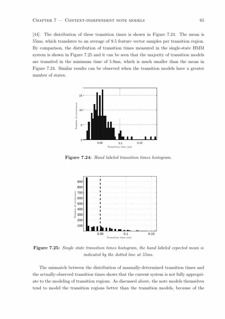
Chapter 7 — Context-independent note models 65
[44]. The distribution of these transition times is shown in Figure 7.24. The mean is
55ms, which translates to an average of 9.5 feature vector samples per transition region.
By comparison, the distribution of transition times measured in the single-state HMM
system is shown in Figure 7.25 and it can be seen that the majority of transition models
are transited in the minimum time of 5.8ms, which is much smaller than the mean in
Figure 7.24. Similar results can be observed when the transition models have a greater
number of states.
15
10
5
00.1 0.150.05
Num
ber
ofoccure
nces
Transition time [ms]
Figure 7.24: Hand labeled transition times histogram.
0.05 0.1 0.15
100
200
300
400
500
600
700
800
900
Num
ber
ofoccure
nces
Transition time [ms]
Figure 7.25: Single state transition times histogram, the hand labeled expected mean is
indicated by the dotted line at 55ms.
The mismatch between the distribution of manually-determined transition times and
the actually-observed transition times shows that the current system is not fully appropri-
ate to the modeling of transition regions. As discussed above, the note models themselves
tend to model the transition regions better than the transition models, because of the

Chapter 7 — Context-independent note models 66
extra cost associated with the pitch feature when transition models are used. One of the
means of addressing this effect is to define the different feature dimensions as separate
input streams, as proposed in the following section.
7.7 Individual feature dimension weighted system
Since significant pitch changes are the key feature within a transition region, the delta-
pitch feature is likely to be dominant within the transition model. It would be undesirable
to have pitch-dependent transition models, since these have to be equally effective regard-
less of the notes surrounding the transition. By discriminating between small, large, up
and down intervals, transitions can be made more specific, while remaining efficient in
terms of the number of transition models that will be sharing the limited training data.
On the other hand, notes are mainly described by their pitch frequency, although
different note stages may also be characterized by delta-pitch. It is important to keep in
mind that the primary note event feature still remains the pitch frequency. A dominant
delta-pitch feature dimension would discriminate among notes in the vicinity of the target
pitch based on pitch intonation. This type of discrimination may not be inclusive enough
of various intervals and styles of singing.
To reflect the differing importance of the features to the transition and to the note
models, we will assign appropriate weights to each feature during Viterbi decoding. If the
current model is a note, the pitch feature is given a larger weighting, thus increasing the
influence that the pitch feature will play in deciding which note model is most likely. The
delta-pitch feature is given a smaller weighting, since the notes are assumed to be largely
delta-pitch independent. For the transition regions the opposite strategy is applied.
The differential weighting of feature vector dimensions is supported within the HTK
toolkit by means of individually weighted data streams [1, pg.71]. Results for such a
weighted system are presented in Table 7.16, while the weighting ratios for the different
model types are given in Table 7.15. Although a decrease in recognition performance
is observed for all systems tested, the occupation times of the transition models have
improved slightly. However, the application of these weights introduces a tendency to
switch between notes and transitions more frequently and at unwanted times. This is
reflected by the greater number of insertions and deletions in Table 7.16. No set of stream
weights could be found to improve the recognition performance relative to an unweighted
system, and therefore the usefulness of this approach remains in doubt.

Chapter 7 — Context-independent note models 67
Model type Pitch feature weight Delta pitch feature weight
Note 1.2 0.8
Transition 0.8 1.2
Table 7.15: Weights applied to the pitch and the delta-pitch features respectively during
Viterbi decoding.
Number of HMM States Accuracy[%] Substitutions Insertions Deletions
1 60.04 439 503 494
2 77.32 172 390 253
3 76.43 168 375 304
4 76.63 161 376 303
5 76.77 164 370 301
6 76.79 170 366 298
Table 7.16: Weighted-feature system performance when using pitch and delta-pitch as
features.
7.8 Chapter summary and conclusion
We began this chapter with a single-state HMM system, then expanded the HMMs to
include between 2 and 6 states in an effort to model the various sequential stages of a
note more accurately. We then developed systems based on first fixing only the pitch
means, and then fixing both the pitch means and variances of the note models to reflect
the exact equally tempered scale frequencies. To improve modelling accuracy, the number
of Gaussian mixtures used by the multi-state system was increased to two and then three
mixtures. In an effort to counter data sparseness without a reduction in the number of
HMM states, tied-state modeling was introduced to the multi-state system. The multi-
state system was then expanded to include explicit transition models to allow a direct
distinction to be made between notes and transition regions. Finally, the transition model
system was modified by adding differential feature dimension weighting. Without the use
of transition models, at least 2 states are required to adequately model notes, and the
inclusion of the delta-pitch feature is only beneficial when 3 or more states are used.
Overall, the systems using parameters optimised on the training data delivered better
performance than those using preset values, which encourages the use of more extensive
data sets in future. Slightly improved robustness to pitch estimation errors could be
obtained by using an increased number of mixtures, but this was not true for systems that

Chapter 7 — Context-independent note models 68
included the delta-pitch features. Finally, consistent overall gains were achieved when
transition models were introduced together with state-tying, and when both pitch and
delta-pitch were used as features. These were the best performing context-independent
systems with note accuracies of almost 85%.

Chapter 8
Context-dependent note and
transition models
8.1 Motivation
One of the greatest challenges in the automatic processing of singing signals is the large
variability between one performer and the next, between one style of music and the next,
and also between one note and the next.
The intonation of a note can be influenced by several factors, including: articulation
context, phrasing context, music tempo and interval context. However, in order to min-
imise data sparseness we have chosen to focus on interval context. The intonation of a
note approached from a higher note differs when the same note is approached from a lower
note. The range of the interval can also have an influence, although generally to a lesser
extent.
The effectiveness of the context-independent transitions introduced in Section 7.6 were
limited by the fact that the models were not pitch-specific. By defining transition models
in terms of specific left and right note contexts, it should be possible to specify a clear
pitch range and thereby improve the accuracy of the model.
8.2 Definition
Context-dependent modeling is a means of creating more specific HMMs by including the
surrounding context in the model definition. One of the most popular ways to introduce
context-dependency is to include the identity of the predecessor as well as the successor
in the model definition. In speech recognition, this leads to so-call “tri-phone” models.
By analogy, we will refer to tri-note models.
Within the speech recognition domain, the context of a specific phoneme would be
determined by the phonemes preceding and following it. In small vocabulary scenarios
69

Chapter 8 — Context-dependent note and transition models 70
with fairly predictable grammar, context-dependency can be applied at word level instead.
This is a closer reflection of the context-dependency implemented in our application.
8.3 Context-dependent note models
Context-dependent HMMs are usually obtained by expanding a base set of initialized
and trained context-independent note models. This is done by initializing each context-
dependent combination with a clone of the corresponding context-independent base note.
Within a musical context the relationship between context-independent and context-
dependent models differs from that between mono-phone to tri-phone models in the sense
that notes are the smallest autonomous components within a musical grammar structure,
whereas phoneme combinations are combined into words and could therefore have a certain
word context-dependency. This general contextual independence of tri-note combinations
relative to each other within a music structure, makes it possible to generate “cross-word”
context-dependent notes.
Firstly the context-independent training-set transcriptions have to be converted to a
context-dependent format. An example of such an expansion is given in Table 8.1. The
table shows how context-dependency is introduced into the note labels, and also how
context-dependent transition models are inserted between notes.
Context-independent labels Context-dependent labels
sil sil
f4 sil-f4+tr
f4-tr+a4
a4 tr-a4+tr
a4-tr+c5
c5 tr-c5+tr
... ...
Table 8.1: An example of context-independent labeling (left) and context-dependent
labeling (right).
One of the disadvantages of applying context-dependency to models is the fact that
the number of models would have to be increased to allow for a different model to be used
in each context. If the available dataset is sparse, many contexts may not have enough or
any data available to be able to train some of the models. Various clustering methods have
proved successful in countering such data sparseness in the interest of realizing context-
dependency. We have a applied one such method termed, decision-tree clustering.

Chapter 8 — Context-dependent note and transition models 71
8.3.1 Decision-tree clustering of context-dependent models
The first step in developing a context-dependent system is to expand the context-indepen-
dent models from a single model to one model for each unique context. This is done
by making copies of the context-independent model for each possible context. Each of
these sets of tri-note models that corresponds to the same base-note is then subjected to
clustering.
A decision-tree is based on a set of questions, which are used to split the tri-note
sets into different contextual groups. The questions are answered by either a “yes” or
a “no”. This allows for a binary hierarchical structuring of the cluster in the form of
a decision-tree. The aim of the clustering algorithm is to find the particular question
that, when used to split a cluster, achieves the greatest improvement in the training data
likelihood. Used within a speech system, a phonetic binary tree would be constructed,
with a single yes-no phonetic question used at each of the nodes. Within our application,
the node questions where designed to discriminate interval context, for example “left up
transition?”, “right silence?” etc. as listed in Table 8.2.
Question description Question description
Left silence? Right silence?
Left up ransition? Right up transition?
Left down transition? Right down transition?
Table 8.2: Decision-tree clustering question set used.
The search for the optimal question is repeated for each newly-subdivided cluster until
the log-likelihood improvement falls below a preset threshold, or the number of training
examples per cluster become too few. When no more subdividing of clusters is allowed,
the leaf nodes of the resulting tree are the clusters of tri-notes that will share the same
HMM and the same training data.
One of the main advantages of using this method is that it allows note combinations
for which there is no training data to be approximated by a cluster which, according to
the decision-tree, has a similar context.
In Figure 8.1 an HMM decision-tree clustering process is illustrated. Binary splitting
is performed through a set of sequential questions, leading to a binary tree structure. The
leaves of the binary tree are the resulting clusters. Tree depth, and hence the number of
context-dependent state sub-clusters per tree, is determined by a log likelihood threshold
variable.
Figure 8.2 provides a schematic overview of the sequential steps that make up the tree-
based clustering method. Firstly the context-independent note models are duplicated so

Chapter 8 — Context-dependent note and transition models 72
L_sil−4
L_up−2
−1R_sil L_dn
−3
R_dn
B4 state 3
noyes
noyesyes
yes yes
no
no no
tru−b4+tru
trd−b4+trusil−b4+sil tru−b4+sil trd−b4+sil
sil−b4+trutrd−b4+trd
Figure 8.1: An illustration of the decision-tree clustering process.
0 5 10
0.05
0.1
0.15
0.2
0.25
−20 0 20 400
0.05
0.1
0.15
0.2
SIL−A6−TRU
0 5 100
0.05
0.1
0.15
0.2
0 5 100
0.05
0.1
0.15
0.2
0 5 100
0.05
0.1
0.15
0.2
0 5 100
0.05
0.1
0.15
0.2
2 4 6 8
0.05
0.1
0.15
0.2
−20 0 20 400
0.05
0.1
0.15
0.2
2 4 6 8
0.05
0.1
0.15
0.2
2 4 6 8
0.05
0.1
0.15
0.2
A4
Training Clone Models
Tree−based Clustering
?
Synthesize
Forward−backward re−estimation
Tree−based clustering
Forward−backward re−estimationof clustered models
Context−dependent clones
Context−independent note
TRU−A4+TRD
TRD−A4+TRU
TRD−A4+TRU TRD−A4+SIL
TRU−A4+TRDTRD−A4+SIL
Viterbi decoding
Recognition result
List of tri−notesnot seen intraining set
TRU−A4+TRD
TRD−A4−TRUTRD−A4+SILTRD−A4+TRU
Figure 8.2: The steps involved in decision-tree clustering of tri-note models.

Chapter 8 — Context-dependent note and transition models 73
that there exists an independent HMM note model for every possible context of a note
present in the training set. With very limited data, it is likely that there will be no training
data for many note combinations that are deemed acceptable by the grammar restrictions
imposed. Based on the decision-tree, and associated set of questions, note combinations
are accommodated by tying them to the appropriate leaf node cluster. This corresponds
to associating unseen tri-notes to seen tri-notes that occur in a similar context. Tying is
applied at a state level, similar to that of the context-independent system described in
Section 7.5. Models within a cluster are all tied implying that the individual states of the
cluster models share the same probability distributions.
This clustering method is designed specifically for single Gaussian state distributions.
This restriction allows for the calculation of the log likelihood for a given cluster of states,
without directly needing the training set of data. The distribution means, variances and
state occupation counts are sufficient for the calculation of this likelihood. Whenever a
state cluster is split into two sets of models (those that satisfy the question requirements
and those that do not), the inevitable increase in log likelihood is calculated and compared
against a threshold parameter. Only cluster splitting that result in an increase greater that
the threshold is allowed. This threshold should be adjusted to allow a sufficient amount
of clusters without allowing clusters with very little training data to exist. Additionally a
minimum occupation threshold exists to limit single outlying states from forming singleton
clusters.
8.3.2 Results
We have conducted a series of experiments using the decision-tree clustering method over a
range of different clustering thresholds for a number of HMM systems. Table 8.3 provides
an overview of the results obtained. The threshold value at which the best recognition
results were obtained is also listed. Low clustering threshold values result in a larger
decision-tree with a larger number of leaves. On the other hand, a high threshold value
would result in a smaller number of clusters and thus the set of HMMs would start to
conform to the context-independent system of Section 7.6. This tendency is reflected in
Figure 8.3.
Figure 8.3 shows how the performance of the system is affected by changing the clus-
tering threshold parameter. It also gives a comparison of this system with that of the
context-independent system. Comparing the context-dependent system to all context-
independent systems, the context-dependent system performs the same or marginally
better, with the average performance increase of 0.41% over the systems mentioned in
Chapter 7. This increase is not substantial, but is consistent for all state topologies.
Since the optimal performance is achieved at higher threshold values, we may suspect,
that there is not enough training data available for many of the note contexts to be ad-

Chapter 8 — Context-dependent note and transition models 74
Number of States Accuracy[%] Substitutions Insertions Deletions Cluster Threshold
1 66.47 541 291 373 1500
2 83.81 182 184 216 700
3 84.86 214 159 171 1000
4 85.11 209 153 173 400
5 84.92 208 157 177 700
6 85.23 199 161 171 1000
Table 8.3: Decision-tree clustered tri-note system performance using pitch and
delta-pitch as features.
equately trained. This suspicion is supported by observations made during some initial
experiments using this decision-tree clustering technique conducted on a much smaller
dataset, and whose results indicated that the context-independent equivalent system al-
ways performed the same or better than the context-dependent system.
8.4 Context-dependent transition models
As mentioned in Section 7.7, the recognition performance of systems using transition mod-
els are adversely affected by the fact that these models employ pitch as a feature but are
expected to be context-independent. This results in poorly-trained and aligned transition
models and transition regions. Using individually weighted features was proposed as a
possible solution to balance the cost between the two types of models in Section 7.7.
However, if the transition models could be adapted to use the pitch feature information
more effectively rather than discard it, it should be possible to achieve better modelling
accuracy in the transition regions. The ideal would be to create fully context-dependent
transition models, (i.e. creating transition models specific to every possible note combina-
tion), but given the limited nature of the available corpus, there is clearly too little data
to train such a set of models explicitly. It is therefore necessary to look at alternative
means of subdividing the generic transition models. In this section we will attempt to
achieve this by synthesizing context-dependent transition models from the parameters of
their left- and right-context note models.
As with the context-dependent note models, we begin by creating a transition model
for each possible note sequence. The model parameters are then adapted and estimated
in different ways, as described in the paragraphs below.

Chapter 8 — Context-dependent note and transition models 75
10 50 200 400 700 150060
65
70
10 50 200 400 700 150082
84
10 50 200 400 700 150082
84
10 50 200 400 700 150082
84
10 50 200 400 700 150082
84
10 50 200 400 700 150082
84
CLUSTERING THRESHOLDR
EC
AC
C[%
]
1 HMM STATE
CLUSTERING THRESHOLD
REC
AC
C[%
]
2 HMM STATES
CLUSTERING THRESHOLD
REC
AC
C[%
]
3 HMM STATES
CLUSTERING THRESHOLD
REC
AC
C[%
]
4 HMM STATES
CLUSTERING THRESHOLD
REC
AC
C[%
]
5 HMM STATES
CLUSTERING THRESHOLDR
EC
AC
C[%
]
6 HMM STATES
Figure 8.3: Decision-tree clustered context-dependent note model system performance
for differing numbers of HMM states, compared to the corresponding context-independent
system performance Section 7.6 indicated by the red dotted horizontal lines.
8.4.1 Reference System
This system will serve as a benchmark for those in the following sections.
fo
fo
TRANSITION NOTE TRANSITION
fo
fo
IDEAL IDEAL
SINGLE SINGLE
SINGLESINGLE
SINGLESINGLE
SINGLESINGLE SINGLE SINGLE
SINGLE SINGLE
SINGLE SINGLE
SINGLE SINGLE
TRAIN
TRAIN
TRAIN TRAIN
IDEAL
TRAIN
µ
σ
µ
σ
Figure 8.4: Reference system modifications to the context-dependent note model clones.
First, a set of context-independent note models is trained using 16 iterations of Baum-
Welsh re-estimation. Next, the pitch means of each state of these models are fixed to
the corresponding ideal equally-tempered frequency value, as was done in Section 7.3.
Additionally, the delta-pitch means and variances of the outer states of note models are
overwritten by those of the centre state. A schematic representation of these modifications
is provided by Figure 8.4. These changes are made so that the models reflect the stable
note regions to a greater extent, and the transition regions to a lesser extent. This should
help to encourage improved transition region modeling and alignment, which is the goal

Chapter 8 — Context-dependent note and transition models 76
of introducing context-dependency with regards to the transition models.
Since this first system will serve as a reference for the following systems, no context-
dependent transition modelling is attempted. Instead a single generic transition model
has been used. The parameters of this transition model were trained using an intermediate
system consisting of a single model for all notes, in addition to the transition model and a
silence model. This intermediate system used only delta-pitch as a feature. Since notes are
associated with small delta-pitch values, while transitions with larger values, this allowed
the training set to be segmented into note and transition regions. This segmentation
was subsequently used to train the single context-independent transition model and the
single context-independent note model using both pitch and delta-pitch as features. After
training the context-independent transition model it is imported to the reference system.
The recognition performance of this system is 73.42%, which is well below most
context-independent systems.
8.4.2 Reference System with global pitch variance
fo
fo
TRANSITION NOTE TRANSITION
fo
fo
IDEAL IDEAL
SINGLE SINGLE
SINGLESINGLE
SINGLESINGLE
SINGLESINGLE SINGLE SINGLE
SINGLE SINGLE
SINGLE SINGLE
SINGLE SINGLE
TRAIN
TRAIN
IDEAL
GLOBAL GLOBALGLOBAL
µ
σ
µ
σ
Figure 8.5: Reference system modifications to the context-dependent note model clones,
with the pitch variance set to the global average.
The system presented here is identical in most respects to that described in the previ-
ous section. A single context-independent transition model has again been used. However
in this case the variances of the pitch feature of all the note models have been overwritten
with the average variance of the notes that are deemed to be “well-trained”. The term
“well-trained” refers to the notes that are seen most frequently in the training set. We have
considered notes to be “well-trained” when there are 200 or more context-independent
instances of the note within the training set. Information regarding the average parameter
values of this set of note models is presented in Table 8.4. A schematic representation of
these modifications is provided by Figure 8.5. The motivation for this substitution stems
from the uncertainty of exactly what region the middle state of a note model is modelling.
For some notes, using the ideal pitch values while maintaining the trained variances, as
was done in Section 8.4.1, may be inappropriate because the trained variances of outer
states may still reflect transition regions while the ideal pitch means no longer do. The
performance of this system is given in Table 8.5.

Chapter 8 — Context-dependent note and transition models 77
Parameter Value
Average delta-pitch standard deviation 1.7975Hz
Average pitch standard deviation 0.5002Hz
Table 8.4: Context-dependent transition model system parameter information. Averate
pitch and delta pitch standard deviations for the 16 note models seen at least 200 times
in the training set.
Number of Training Iterations Note Accuracy [%]
0 82.89
1 86.02
Table 8.5: Reference system performance when using a global pitch variance.
A notable improvement is evident from the results in Table 8.5. The pitch variance
adjustments seem to have assisted in establishing note models that are dedicated to the
modeling of note events only. Also, the improvement after a single training iteration of
these models shows that there are small but significant differences between the models
due to their contextual-dependency. This is a promising sign suggesting that with more
data the results using the technique could improve significantly. Further re-estimation
iterations did not lead to additional improvement.
8.4.3 Two transition model system
fo
fo
TRANSITION NOTE NOTE
fo
fo
IDEAL IDEAL IDEAL IDEALIDEAL
GLOBAL GLOBAL
IDEAL
GLOBALGLOBAL GLOBAL GLOBAL
TRAIN
TRAIN
TRAIN
TRAIN
TRAIN TRAIN
TRAIN TRAIN
µ
σ
µ
σ
Figure 8.6: Context-dependent transition model synthesis steps.
We now modify the system implemented in Section 8.4.2, by overwriting the pitch
values of the transition models with those of the neighboring note outer states. These
steps are depicted in Figure 8.6. The single generic transition model is replaced by a
generic up transition and generic down transition model depending on the surrounding
notes of the transition. The up and down transition models have been trained in a similar

Chapter 8 — Context-dependent note and transition models 78
fashion to the single generic transition model described in the previous section. The
results for this system are presented in Table 8.6.
Number of Training Iterations Note Accuracy [%]
0 70.82
1 83.14
Table 8.6: Two transition model modified system.
To investigate this unexpected 2.88% drop in performance, relative to the system in
Section 8.4.2, each of the changes between the two systems are evaluated separately. By
comparing identical systems using the two transitions versus those using only the single
transition, it was determined that most of the performance drop could be contributed
to the transition model pitch parameter modification, or the use of “synthesized” fully
context-dependent transition models.
Further investigation, however revealed that the main problem with the procedure
was the setting of the outside state pitch variances of the transition models to a standard
deviation of 0.5 semitones. An identical two transition model system using the same
transition model pitch parameter modification, but without setting the outside state pitch
variances1, performed very similar to that of Section 8.4.2, with a small performance drop
of only 0.52% in transcription accuracy. This result concurs with the context-independent
case in Section 7.3, where the presetting of pitch variances was also unsuccessful, and also
with the findings of preliminary tests, where varying between a single transition model
and an up and a down transition model did not alter the performance greatly.
fo
fo
TRANSITION NOTE NOTE
fo
fo SINGLE SINGLE
IDEAL IDEAL IDEAL IDEALIDEAL
GLOBAL GLOBAL GLOBAL
IDEAL
GLOBALGLOBALGLOBAL
TRAIN
TRAIN
TRAIN
TRAIN
TRAIN
TRAIN
TRAIN
TRAIN
µ
σ
µ
σ
Figure 8.7: Context-dependent transition model synthesis steps.
In view of these findings, a system similar to that described above, but setting the
transition model pitch variance to the trained single transition model pitch variance in-
stead of the global variance, has been created and tested. In other words, the system
is similar to that of Section 8.4.2, but with the synthesis procedure applied to the pitch
1i.e. only the transition model pitch means were set.

Chapter 8 — Context-dependent note and transition models 79
mean variable of the context-dependent transition models states only. Figure 8.7 provides
a illustration of modifications. The results are shown in Table 8.7.
Number of Training Iterations Note Accuracy [%]
0 83.17
1 86.66
Table 8.7: Two transition model modified system without pitch variances being set.
These results seem to indicate that the synthesized transitions are not only useful
with transition region alignment, but can also improve the system’s performance. It can
also be concluded that the pitch variance of the transition models should be left fairly
generic. The fact that the system performance increases by almost 5% when the transition
variances are left equal to those of the generic transition model (i.e. very broad) indicates a
high variability not only in the transition regions, but also in the voice as instrument. The
improvement after only a single training iteration is likely to occur since the transitions
models have been altered significantly, but also emphasizes the fact that this method can
be exploited further given a larger training set.
0.05 0.1 0.15 0.2 0.25 0.3 0.350
50
100
150
200
250
Time [seconds]
Num
ber
ofoccurr
ences
Figure 8.8: Histogram of transition times of the synthesize transition region system.
Furthermore, the transition times associated with the context-dependent transition
models are distributed as shown in Figure 8.8. A comparison with Figure 7.24 reveals
that this distribution is much closer to that which is observed in hand-labelled data,
which indicates that the transition regions are modelled more accurately by the context-
dependent models.
Figure 8.9 compares the segmentation into notes and transitions achieved by a system
using context-independent transition models with a system using context-dependent tran-
sition models. The context-independent transition models lead to very narrow transition
regions, while the context-dependent transition models result in a segmentation in which
transitions are more accurately identified.

Chapter 8 — Context-dependent note and transition models 80
0 0.5 1 1.5 2
70
72
74
76
78sil b4 d5s f5s d5s b4
0 0.5 1 1.5 2
70
72
74
76
78sil b4 d5s f5s d5s b4
Xpitch
ref
score
Time [seconds]
Mid
iN
um
ber
Time [seconds]
Mid
iN
um
ber
Figure 8.9: Transition region recognition alignment comparison of a
context-independent transition model system (top) and context-dependent transition
models (bottom). Note regions are indicated by shaded blocks, and transition regions are
unshaded.

Chapter 8 — Context-dependent note and transition models 81
8.5 Chapter summary and conclusion
In this chapter we have expanded the context-independent systems, so that the possible
effects that the preceding and following note or transition may have on the note or transi-
tion being modeled may be incorporated into the modeling process. We have introduced
context-dependent note modeling by means of a decision-tree clustering method, and
context-dependent transition modeling by means of various parameter adaptation and es-
timation schemes. Both sets of experiments yielded approximately equal or slightly better
results than the best results obtained by the context-independent systems in Chapter 7.
Improved segmentation of transition regions was however achieved with the introduction
of context-dependent transition models.
The limited amount of training data does not allow for fully context-dependent mod-
eling of either the notes themselves or the transition models. Furthermore, decision-tree
clustering experiments have shown that the best recognition accuracy is often obtained
when the number of clusters is very small. This suggests that, given more training data, a
greater variety of sufficiently trained interval-contexts (i.e. a greater number of transition
models) could be produced, and the full advantages of this method could be explored.
By increasing the size of the training set especially with respect to the higher and lower
notes and by creating a sufficient variety of note combinations, transitions can be defined
not only by interval size but by the actual note combinations. Context-dependency in
terms of tonality or scale related context may also be used in future as additional context-
dependent descriptors.

Chapter 9
Development of a sight-singing tutor
9.1 Introduction
The aim of a sight-singing tutor is to provide some sort of feedback to help the user assess
the accuracy of his or her singing. Figure 9.1 shows the user feedback generated by one
such system. The reference melody is displayed on the screen and the user is then asked
to sing the melody as accurately as possible. The user’s note sequence is matched against
the reference melody sequence using, in this case, a dynamic programming algorithm. A
global score is calculated based on note duration accuracy as well as pitch accuracy.
Figure 9.1: An example of user feedback generated by an existing sight-singing tutor
due to McNab et al [27]. The note sequence on top is the reference melody and the
bottom note sequence is the user’s attempt.
Figure 9.2 provides an illustration of a note-level sight-singing tutor system in more
detail than the conceptual Figure 1.1 in Section 1.2. Figure 9.2 illustrates how the au-
tomatic transcription system developed in Chapters 7 and 8 serves as front-end to the
sight-singing tutor module. Most sight-singing tutor research projects [49, 48] as well as
commerical sight-singing tutor systems [40] generate user feedback on a frame-by-frame
level. This means that the pitch is estimated and shown together with the current target
note and pitch in real-time. Only one system, due to McNab et al [27], was found to
perform individual note segmentation and scoring. However, in this case the input was
82

Chapter 9 — Development of a sight-singing tutor 83
restricted to \ta or \da. Depending on how legato the note passage is sung, this pronun-
ciation restriction forces a brief interruption of airflow and consequently tends to promote
staccato articulation. This in turn shortens the length of transition regions or eliminates
them altogether, thereby avoiding the need to model these problematic segments.
. . .
. . .
. . .
fo
. . .
. . .
Note2 Duration
Pitch NoteN Duration
PitchNote1 Duration
PitchTRANSCRIPTION
REFERENCE
OF EXERCISE
fo fo fo fo
4 4.2 4.4 4.6 4.8 5 5.2 5.4 5.6
x 104
−0.1
−0.05
0
0.05
0.1
AM
PLI
TU
DE
. . .
fo
FEATURE VECTORS
SAMPLE NUMBER
HMMs andViterbi
search
. . .
NOTE SEGMENTATION &
RECOGNITION
EVALUATION
OUTPUT SCORE
TRANSCRIPTIONMODULE
TUTOR
ACOUSTIC MODEL
FRONT−END
MODULE
fo fo fo fo
. . .
ACOUSTIC SIGNAL
FR
AM
E 0
FR
AM
E 1
Figure 9.2: A block-diagram illustration of a sight-singing tutor system.
In the rest of the chapter, we develop a sight-singing tutor system based on note-level
scoring that is not limited to certain pronunciations. This system will incorporate the
statistical modelling approaches presented in the previous chapters.
9.2 Automatic evaluation of singing quality
To develop a sight-singing tutor system, we have implemented two evaluation strategies.
The first tries to represent ideal transition regions by means of various parametric func-
tions. The second explicitly identifies and then eliminates these transition regions, and
therefore scores only the notes. For both approaches we evaluated the quality of sung
notes by calculating the deviation of the user’s pitch from it’s ideal value, as obtained
from the reference transcription.

Chapter 9 — Development of a sight-singing tutor 84
Let a sequence of N notes be denoted by the symbols n0, n1, · · · , nN−1. For this
sequence of notes, a sequence of M pitch estimates p0, p1, · · · , pM−1, one per frame, is
made from the recorded acoustic data. Assume that the start and end frames of each
note ni are given by αi and βi respectively, such that 0 ≤ αi < βi ≤ M − 1. Hence the
pitch estimates for note ni are pαi, pαi+1, · · · , pβi
. Finally, let the true pitch for a note
ni be pni. The quality with which note ni is sung by the subject is then quantified by
Equation 9.1 as Ei:
Ei =1
βi − αi + 1
βi∑
j=αi
|pni− pj| (9.1)
This is the per-frame average deviation of the estimated pitch pj from the correct
reference pitch pniover the duration of the note. The difference is calculated in the MIDI
domain so that the deviation is linear and easier to interpret.
By placing heavy restrictions on the permitted pronunciation of the user, R.Mcnab et
al [27] were able to avoid considering the effects of transition regions on the evaluation
process. However for our system these restrictions do not apply, so the transition regions,
which are more variable than the notes, must be negotiated in some way during the
scoring process. We have followed two approaches: The first method tries to model
the transition regions explicitly using parametric models. The second method eliminates
the transition regions from the scoring process. In both cases the improved alignment
accuracies described in Section 8.4 are very important.
9.2.1 Segmentation by forced alignment
For both approaches introduced in the previous section, we have determined the melody
transcription of the user input using the system described in Section 8.4.3, since the notes
were most accurately modeled and the transition regions most accurately defined by this
particular system.
Instead of normal note recognition, where the sequence of notes that has been sung is
unknown and must therefore be determined using HMM note models and a Viterbi search,
for the sight-singing tutor the transcription of the target melody is known in advance.
When this known sequence of notes is used to restrict the Viterbi search, the process
is known as a forced alignment. Essentially the note sequence is fixed, and the Viterbi
search is used only to find the optimal start and end times for each HMM model, i.e.
the segmentation of the sequence features into notes and transitions. This process can be
viewed as a time-alignment between the sequence of features and the sequence of notes.
It results in a set of instances at which one HMM transits to the next for a particular
audio signal.

Chapter 9 — Development of a sight-singing tutor 85
.
.
.
.
.
.
.
.
.
.
.
.
.
.
.
.
.
.
.
.
.
.
.
.
.
.
.
.
.
.
.
.
.
.
.
.
.
.
.
.
.
.
.
.
.
.
.
.
.
.
.
.
.
.
.
.
.
4 4.2 4.4 4.6 4.8 5 5.2 5.4 5.6
x 104
−0.1
−0.05
0
0.05
0.1
NOTE 1 TRANS NOTE 2 TRANS NOTE 3
start
Note Sequence
Audio Signal
Feature Vectors
Reference
Corresponding
Sequence of
HMMs
end
FR
AM
E 1
Time
AM
PIT
UD
E
SAMPLE NUMBER
. . .FR
AM
E 0
Figure 9.3: An illustrative example of segmentation by forced alignment.

Chapter 9 — Development of a sight-singing tutor 86
An illustrative example of the forced alignment segmentation method is shown in
Figure 9.3. It illustrates how the feature vectors extracted from the input audio signal
are grouped and aligned to the known sequence of note and transition HMMs, thereby
accomplishing segmentation of the audio signal based on the reference note sequence.
9.2.2 Parametric models for note transitions
The first scoring approach involves modeling the transition regions explicitly so that no
voiced part of the pitch track is discarded in the scoring process. However, scoring is
still performed on a note-by-note basis. For this scoring method we have defined each
note segment to extend from the beginning of the note to the beginning of the next
note, thus including the transition following the note being scored. We have considered
two parametric functions with which to approximate the pitch contour in the transition
regions.
Step transition contour
The first and most simple approach was to approximate the transition by a step function
which jumps discontinuously at note boundaries. It can be defined as:
Tt =
{
0 if t < 0
1 if t ≥ 0
T ∗t = Tt × (pni+1
− pni) + pni
(9.2)
For downward transitions, the unit step function is reversed so that the starting value
of the unit step function is 1 and the ending value is 0. The unit step function Tt, is scaled
by the difference in pitch between the two successive notes pni+1− pni
, and the pitch of
the first note pniis added as offset so that the scaled step function T ∗
t , starts at pitch
frequency pniand ends at pni+1
. An example of the unit and scaled functions is given in
Figure 9.4.
Cosine transition contour
Secondly, we have modeled transition regions using half a period of the cosine function.
We have defined our generic function, Ct to again span the frequency interval [0, 1]:
Ct =1
2cos(t) +
1
2(9.3)

Chapter 9 — Development of a sight-singing tutor 87
−8 −6 −4 −2 0 2 4 6 8
0
0.2
0.4
0.6
0.8
1
−8 −6 −4 −2 0 2 4 6 8
72
73
74
75
76
Time [samples]
MID
IN
um
ber
Time [samples]
MID
IN
um
ber
pni
pni+1
Figure 9.4: An illustrative example of the unit step function (top) and the scaled step
function (bottom). The notes preceeding and following the transition are indicated by pni
and pni+1respectively.
We have chosen the angle t to range from 0 to π, and have scaled this to correspond
to the duration of the transitions. Figure 9.6 gives an example of each transition model.
Again the unit curve Ct is scaled as shown in Equation 9.4 so that the transition curve
starts at the pitch frequency of the previous note pni, and end at the pitch frequency of
the next note pni+1:
C∗t = Ct × (pni+1
− pni) + pni
(9.4)
By choosing the angle t to start at 0 and end at π the generic cosine function, as
defined in Equation 9.3 is guaranteed to start and end at to 0 and 1 respectively. As
for the unit step function, for downward transitions, the function is reversed so that the
starting value is 1 and the ending value is 0. An example of the cosine approximation
used is shown in Figure 9.5. A transition region example together with the pitch track
and various transition contour estimation models are shown in Figure 9.6.
Figures 9.7 and 9.8 show the step and cosine approximations respectively being used to
model a pitch track. The scores shown in the bottom graphs are the per-sample average
note semitone errors. As was expected, the cosine model is a better approximation of
the transition region and therefore penalises these less severely. Although the preceding
and trailing silences of the melody example are included in all figures, they have not
contributed to the scoring.
To accommodate the pitch track instability associated with silence-to-note transitions
and vice versa, we have applied a heuristic rule which excludes the first or last 3 pitch

Chapter 9 — Development of a sight-singing tutor 88
−10 −8 −6 −4 −2 0 2 4 6 8 100
0.2
0.4
0.6
0.8
1
−10 −8 −6 −4 −2 0 2 4 6 8 1072
73
74
75
76
Time [samples]
MID
IN
um
ber
Time [samples]
MID
IN
um
ber
pni
pni+1
Figure 9.5: An illustrative example of the unit cosine curve (top) and the scaled cosine
curve (bottom). The notes preceeding and following the transition are indicated by pni
and pni+1respectively.
0.42 0.44 0.46 0.48 0.5 0.52 0.54 0.56 0.58 0.6
71
72
73
74
75
76
77
78
Transition region
pitchstepcosine
Time [seconds]
MID
IN
um
ber
pnipni+1
Figure 9.6: An illustrative example of the two approaches to transition region
modelling. The transition region is indicated by the unshaded area. The notes preceeding
and following the transition are indicated by pniand pni+1
respectively.

Chapter 9 — Development of a sight-singing tutor 89
samples of the affected note, depending on whether it borders on a preceding or trailing
silence. These notes would otherwise be penalized disproportionately for those short pitch
track deviations from the target frequency.
0 0.2 0.4 0.6 0.8 1 1.2 1.4 1.6 1.8 270
75
80
user pitchblock reference
0 0.2 0.4 0.6 0.8 1 1.2 1.4 1.6 1.8 2
−2
0
2
0.2 0.4 0.6 0.8 1 1.2 1.4 1.6 1.8 20.20.40.60.8
11.2
0.470.57 0.49 0.42 0.41
Time [seconds]
MID
IN
um
Time [seconds]
MID
IN
um
Time [seconds]
MID
IN
um
Figure 9.7: An illustrative example of note scoring where transition regions are
included in the scoring process and approximated using a step function. The pitch track
and reference transcription are shown in the top graph, pitch track deviation from the
reference in the middle, and the average per-sample MIDI semitone deviation from the
correct pitch in the bottom bar chart. The numerical MIDI semitone deviation per
sample figures are also shown in the bottom graph.
9.2.3 Exclusion of transition regions from note scores
As an alternative to explicit parametric modelling of the transition regions, we can simply
omit these from the scoring process and focus only on the stable parts of the notes. This
approach is illustrated in Figure 9.9, notes are indicated by gray shading, while transition
regions are not shaded. The segmentation into notes and transition regions is once again
obtained by means of a forced alignment with the reference transcript.
The inherent frequency variation during vibrato is still a concern with respect to the
current scoring method. Vibrato is an aspect that has not been addressed in this work
and remains the subject of a future investigation.

Chapter 9 — Development of a sight-singing tutor 90
0 0.2 0.4 0.6 0.8 1 1.2 1.4 1.6 1.8 270
75
80
user pitchcosine reference
0 0.2 0.4 0.6 0.8 1 1.2 1.4 1.6 1.8 2
−2
0
2
0 0.2 0.4 0.6 0.8 1 1.2 1.4 1.6 1.8 20
0.5
1
1.5
0.47 0.560.42
0.31 0.41
Time [seconds]
MID
IN
um
Time [seconds]
MID
IN
um
Time [seconds]
MID
IN
um
Figure 9.8: An illustrative example of note scoring where transition regions are
included in the scoring process and approximated using a cosine function. The pitch
track and reference transcription are shown in the top graph, pitch track deviation from
the reference in the middle, and the average per-sample MIDI semitone deviation from
the correct pitch in the bottom bar chart. The numerical MIDI semitone deviations are
also shown in the bottom graph.
As is evident in the melody example, the transition regions are very hard to accurately
model using a single function. This can be observed by comparing the much larger
magnitude pitch track deviation from the reference transcription in the transition regions
to that of the note regions in Figures 9.7 and 9.8. It is therefore easy to see why the
method that scores note regions only produces smaller note penalty scores. This method
of scoring appears to be more accurate, considering the variability of transition regions.
9.3 Conclusion and future possibilities
We have investigated two different evaluation strategies for the realisation of a sight-
singing tutor. The first estimates the transition regions and including them together with
the notes in the scoring process, the second eliminates the transition regions from the
scoring process and only scores the notes.

Chapter 9 — Development of a sight-singing tutor 91
0 0.2 0.4 0.6 0.8 1 1.2 1.4 1.6 1.8 270
75
80
user pitchblock reference
0 0.2 0.4 0.6 0.8 1 1.2 1.4 1.6 1.8 2
−2
0
2
0 0.2 0.4 0.6 0.8 1 1.2 1.4 1.6 1.8 20
0.5
1
1.5
0.30.5
0.340.15
0.41
Time [seconds]
MID
IN
um
ber
Time [seconds]
MID
IN
um
ber
Time [seconds]
MID
IN
um
ber
Figure 9.9: An illustrative example of note scoring where transition regions are omitted
in the scoring process. Only pitch track regions withing the gray blocks were used in the
scoring process. The top figure shows the pitch track of the user against a step reference
transcription. The middle graph is the difference between the user pitch track and the
reference set to 0 in the transition regions. The average per-sample MIDI semitone
deviation from the correct pitch is shown in the bottom bar chart. The numerical MIDI
semitone deviations are also shown in the bottom graph.
The method which excludes transition regions in the scoring process appears to be
the more useful evaluation method. However, it must be said that the concept of singing
accuracy is to a large extent perceptual, and further investigation and testing with the
help of expert opinions is needed. In particular, the nature of an ideal sung passage, as well
as the severity of different types of deviations from the ideal, must be better understood.
The scoring metrics can then be updated accordingly. This however fell beyond the scope
of the current work.
Future possibilities include defining more advanced scoring criteria, which may in-
clude vibrato modeling and other intonation tendencies, to improve the accuracy of the
evaluation algorithm. For example, by taking into account the effect that the preceding
and trailing transitions may have on the intonation of a particular note, the pitch target
may be altered, especially at the start and end of the note to allow for subtle acceptable

Chapter 9 — Development of a sight-singing tutor 92
intonation deviations.

Chapter 10
Final summary and conclusions
We have developed a note-level sight-singing tutor system, which is able to achieve accu-
rate time-alignment of notes and transition regions, by means of the forced alignment of
suitably-trained hidden Markov models. The system is based on a context-dependent note
and transition transcription system, and achieves a note recognition accuracy of around
86%.
Apart from the assembly of a singing corpus consisting of 26 soprano voices and a
total of 13842 notes, spanning 30 semitones ranging from A3 to D6♯, several techniques
and modeling topologies, new to the singing-transcription field, are introduced.
Various hidden Markov model (HMM) topologies have been used to model the notes,
silences and transition regions between notes. A non-repetitive grammar is used to allow
for any combination of notes except direct repetitions of the same note.
Starting with context-independent note models, we have started with a single-state
system. When using a single-dimensional pitch feature in this system, it was found that
the number of states have been increased to between 2 to 6 states for optimal performance.
The addition of extra states created an opportunity for the note models to model the
transition regions independently of the stable note regions. This improved ability in
capturing the time-varying characteristic properties of the notes was reflected in the large
increase in transcription accuracy, especially when the delta-pitch feature was added.
These multi-state systems, which had been trained on the compiled corpus, are then
compared to similar systems in which the Gaussian state parameters are set to their ex-
pected theoretical values. When presetting only the means, the overall note accuracy
marginally improved. When setting also the variances in this way, performance deterio-
rated. This is an indication that appears to encourage the use of training data for the
determination of model parameters.
The context-independent multi-state system has also been expanded to include more
Gaussian mixtures per state. This was done especially to help absorb insertion errors,
which may occur due to pitch estimate errors such as pitch doubling. A small but consis-
tent transcription accuracy gain is observed for both the two-mixture and three-mixture
93

Chapter 10 — Final summary and conclusions 94
systems.
In an effort to maximize the usage efficiency of the training data, improve the modeling
of transition regions, as well as extend the minimum duration of HMMs while avoiding
the undertraining of added states, a technique known as state-tying has been applied to
the multi-state system. A large reduction in deletion errors was observed and this resulted
in improved transcription accuracy.
The increased note model variance, due to the implicit modeling of transition regions
by notes, motivated the introduction of explicit transition models. HMMs identical in
structure to the note models are used to model to pitch transition from one stable note
region to the next stable note region. In an effort to extend the minimum transition
duration, state-tying is then applied to the transition model system. Individual feature
dimension weighting was also applied to the transition model system, but this resulted in
an unstable switching between note and transition models and thus a significant deterio-
ration in system performance.
The introduction of context-dependent note models showed that a small but consistent
gain can be achieved by performing tree-based clustering. The small number of clusters
seems to suggest that more data would help to improve the effectiveness of this approach.
The pitch-dependency of the context-independent transition models, prompted the in-
troduction of pitch-specific context-dependent transition models which ultimately resulted
in the best performing system, with 86.66% note transcription accuracy. Furthermore,
for this same system the time-alignment of notes and the transitions between notes, an
important aspect for a note-level tutoring system, was also significantly improved.
Based on the context-dependent transition models, a sight-singing tutor system which
calculates the semitone-per-sample deviation of the pitch track from the target note, was
implemented. Although some methods of including the transition regions were proposed,
the exclusion of the transition regions from the scoring process appeared to be a more
useful way of providing note-based accuracy feedback.
10.1 Contributions
In conclusion, the following aspects of this project can be considered contributions to the
field of music processing, since they have to our knowledge not been reported elsewhere:
• The assembly of an annotated dataset containing 26 soprano voices.
• The introduction of explicit transition modelling.
• The introduction of context-dependency with regards to note models and transition
models.

Chapter 10 — Final summary and conclusions 95
• The evaluation of preset Gaussian parameters, individual feature dimension weight-
ing, as well as tree-based clustering.
• The demonstration of a pronunciation-independent note-level sight-singing tutor
system.
10.2 Future implementations
Finally, there are several directions in which this project could be extended, that fell
beyond its scope due to time limitations. Some of these are:
• Including a musicological model which assigns different transition probabilities ac-
cording to the likelihood of each particular transition within the musical key.
• Including additional features, such as the energy intensity or the degree of voicing.
• Including vibrato modeling.
• Extending the training set sufficiently so that fully context-dependent modeling
becomes feasible.
• Defining a more advanced note scoring criteria.

Bibliography
[1] “The HTK Book, version 3.0.” April 2000.
[2] BAUM, L. E., “An inequality and assosiated maximization technique in statistical
estimation for probability functions of Markov processes.” Inequalities, 1972, Vol. 3,
pp. 1–8.
[3] BELLO, J., MONTI, G., and SANDLER, M., “Techniques for Automatic Music
Transcription.” in Automatic Music Transcription, in International Symposium on
Music Information Retrieval, 2000.
[4] BRANDAO, M., WIGGINS, G., and PAIN, H., “Computers in Music Education
Symposium on Musical Creativity.” in Proceedings of the AISB, 1999.
[5] CAMBOROPOULOS, E., Towards a General Computational Structure of Musical
Structure. PhD thesis, Faculty of Music, University of Edinburgh, 1998.
[6] CANO, P., “Fundamental Frequency Estimation in the SMS Analysis.” DAFX
Proceedings, 1998.
[7] CANO, P., LOSCOS, A., and BONADA, J., “Scoreperformance matching using
HMMs.”
[8] CLARISSE, L. P., MARTENS, J. P., LESAFFRE, M., BAETS, B. D.,
MEYER, H., and LEMAN, M., “An auditory model based transcriber of singing
sequences.” in Proceedings of 3rd International Conference on Music Information
Retrieval, ISMIR ’02, May 2002.
[9] DAHLIG, E., “EsAC database: Essen associative code and folksong database.”
1994.
[10] DANNENBERG, R., SANCHEZ, M., JOSEPH, A., CAPELI, P., JOSEPH, R., and
SAUL, R., “A computer-based multi-media tutor for beginning piano students.”
[11] DELLER, J. R., PROAKIS, J. G., and HANSEN, J. H. L., Discrete-time processing
of speech signals . New York: MacMillan Publishing Co., 1993.
96

BIBLIOGRAPHY 97
[12] ED. SCHOLES, P., “Oxford Companion to Music.” Comput. Methods Appl. Mech.
Engrg., 1955, Vol. 19th edition, p. 291.
[13] FUJISAKI, W. and KASHINO, M., “Contributions of temporal and place cues in
pitch perception of absolute pitch possessors.” Perception & Psychophysics,
February 2005, Vol. 67, pp. 315–323.
[14] GHIAS, A., LOGAN, J., CHAMBERLIN, D., and SMITH, B. C., “Query by
Humming: Musical Information Retrieval in an Audio Database.” in ACM
Multimedia, pp. 231–236, 1995.
[15] HELMHOLTZ, H., On the Sensations of Tones . New York: Dover, 1954.
[16] HESS, W., Pitch Determination of Speech Signals . Berlin: Springer-Verlag, 1983.
[17] HOFSTETTER, F., “Computer-based aural training: The GUIDO system.” in
Journal of Computer-Based Instrucion, vol. 7(3), p. 8492, 1981.
[18] IMMERSEEL, L. V. and MARTENS, J., “Pitch and voiced/unvoiced determination
with an auditory model.” in J. Acoust. Soc. Am.,91, pp. 3511–3526, 1992.
[19] KAWAHARA, H. and DE CHEVEIGNE, A., “Yin, a fundamental frequency
estimator for speech and music.” in J. Acoust. Soc. Am.,111(4), pp. 1917–1930,
April 2002.
[20] KELSEY, F., Foundations of Singing . London: Williams & Norgate, 1950.
[21] KLAPURI, A., “Automatic transcription of music.” Master’s thesis, Tampere
University of Technology, Department of Information Technology, 1998.
[22] KUMAR, P., JOSHI, M., DUTTA-ROY, H. S., and RAO, P., “Sung note
segmentation for a query-by-humming system.”
[23] KUO, C.-C. J., SHIH, H.-H., and NARAYANAN, S. S., “An HMM-based approach
to humming transcription.” in Proceedings of IEEE International Conference on
Multimedia and Expo, vol. 1, pp. 337–340, 2002.
[24] L.R. RABINER, A. R., M.J. CHENG and MCGONEGAL, C., “A comparative
performance study of several pitch detection algorithm.” IEEE Trans. Acoust.,
Speech and Signal Processing, 1976, Vol. ASSP-24(5), pp. 399–418.
[25] MALMKJAER, K., The Linguistics Encyclopedia. London and New York:
Routledge, 1991.

BIBLIOGRAPHY 98
[26] MATTHAEI, P. E., “Automatic music transcription an exploratory study.”
Master’s thesis, University of Stellenbosch, April 2004.
[27] MCNAB, R., SMITH, L., and WITTEN, I., “Signal processing for melody
transcription.” in Proc. 19th Australasian Computer Science Conf., (Melbourne),
pp. 301–307, January 1996.
[28] MEEK, C. and BIRMINGHAM, W., “Johnny Cant Sing: A Comprehensive Error
Model for Sung Music Queries.” in Proceedings of the Third International
Symposium on Music Information Retrieval (ISMIR), (Melbourne), pp. 124–132,
2002.
[29] M.RYYNANEN and KLAPURI, A., “Probabilistic Modelling of Note Events in the
Transcription of Monophonic Melodies.” in Proc. ISCA Tutorial and Research
Workshop on Statistical and Perceptual Audio Processing, (Tampere), 2004.
[30] O’SHEA, T. and SELF, J., “Learning and Teaching with Computers.” in Journal of
Computer-Based Instrucion, (London: Prentice-Hall), 1983.
[31] PAUWS, S., “CubyHum: A fully operational Query by Humming System.” in
Proceedings of the Third International Conference on Music Information Retrieval,
ed. Michael Fingerhut, (Paris: IRCAM, Centre Pompidou), pp. 187–196, 2002.
[32] PISZCZALSKI, M., “A Computational Model for Music Transcription.” Master’s
thesis, University of Stanford, 1986.
[33] POLLASTRI, E. and HAUS, G., “An audio front end for query by humming
systems.” 2001.
[34] POLLASTRI, E., “Some considerations about processing singing voice for music
retrieval.” in Proceedings of 3rd International Conference on Music Information
Retrieval, ISMIR ’02, October 2002.
[35] PRAME, E., “Vibrato extent and intonation in professional Western lyric singing.”
in Acoustical Society of America, (Department of Speech, Music, and Hearing,
Royal Institute of Technology (KTH), Stockholm, Sweden), March 1997.
[36] RABINER, L. R., “A tutorial on hidden Markov models and selected applications
in speech recognition.” Proceedings of the IEEE, 1989, Vol. 77, No. 2, No. 2,
pp. 257–286.
[37] REISS, J. D. and WIGGINS, G. A., “What You See Is What You Get: On
Visualizing Music.” in Proceedings of ISMIR 2005: The Sixth Conference on Music
Information Retrieval, Ed., 2005.

BIBLIOGRAPHY 99
[38] ROMA, L., The Science and Art of Singing . New York: G. Schirmer, Inc., 1956.
[39] ROSS, M. J., SHAFFER, H. L., COHEN, A., FREUDBERG, R., and
MANLEY, H. J., “Average magnitude difference function pitch extractor.” in IEEE
Transactions on Acoustics, Speech and Signal Processing, vol. 22nd edition,
pp. 353–362, 1974.
[40] SAUL, K., LEE, D., ISBELL, C., and LECUN, Y., “Real time voice processing
with audiovisual feedback: toward autonomous agents with perfect pitch.” 2002.
[41] SCHMIDT, J., Basics of Singing . New York: Schirmer Books, 1984.
[42] SETHARES, W. A., Tuning, timbre, spectrum, scale. Second edition. London:
Springer, 2005.
[43] SHIH, H., NARAYANAN, S., and KUO, C.-C. J., “Multidimensional humming
transcription using a statistical approach for query by humming systems.” in
International Conference on Multimedia and Expo, ICME ’03, vol. 3, pp. 385–388,
July 2003.
[44] SJOLANDER, K. and BESKOW, J., “Wavesurfer audio editing software version
1.8.5.” 2005.
[45] UNISA, Unisa singing examination syllabuses. University of South Africa,
May 2001.
[46] VERCOE, B. L., GARDNER, W. G., and SCHEIRER, E. D., “Structured audio:
creation, transmission, and rendering of parametric sound representations.” in
Proceedings of the IEEE, vol. 86, pp. 922–940, May 1998.
[47] VIITANIEMI, T., KLAPURI, A., and ERONEN, A., “A probabilistic model for the
transcription of single-voice melodies.” in Proceedings of the 2003 Finnish Signal
Processing Symposium, pp. 59–63, May 2003.
[48] WELCH, G. F., HOWARD, D. M., HIMONIDES, E., and BRERETON, J.,
“Real-time feedback in the singing studio: an innovatory action-research project
using new voice technology.” Music Education Research, July 2005, Vol. 7, No. 2,
pp. 225–249.
[49] WILSON, T. C. W., P. and CALLAGHAN, J., “Looking at singing: Does real-time
visual feedback improve the way we learn to sing?.” in 2nd APSCOM Conference :
Asia-Pacific Society for the Cognitive Sciences of Music, (Seoul, South Korea),
2005.

Appendix A
Appendix
A.1 Yin algorithm code optimization
In the sections that follow, we will firstly attempt to show how the Yin algorithm has
been implemented in Matlab. Equation A.1 shows the squared difference function:
dt(τ) =
t+W∑
j=t
(xj − xj+τ )2 (A.1)
The Yin function as previously defined, is:
d′
t(τ) =
{
1 τ = 0
dt(τ)/[( 1τ)∑τ
j=1 dt(j)] otherwise(A.2)
The definitions of the symbols used in the equations are explained in more detail in
Section 5.1. Figures A.1 and A.2 illustrate how the mathematical formula in Equations
A.1 and A.2 of the Yin algorithm have been implemented in Matlab. The code written
in Figure A.1 is a direct implementation of the equations while that in Figure A.2 is
optimized and makes use of matrix multiplication rather than multiple loops. A
stepwise code-to-mathematical formula correspondence of the code presented in Figure
A.2 is presented in Section A.1.
In both Figures A.1 and A.2, the code segment labeled as section A corresponds to
Equation A.1, the code labeled as section B corresponds to Equation A.2 when τ = 0,
and the code labeled as section C corresponds to the rest of Equation A.2.
Equations A.3 to A.9 provide a mathematical formulation of the Matlab code shown in
Figure A.2. Lines 1 to 7 as indicated in Figure A.2 correspond to Equations A.3 to A.9
respectively.
100

Chapter A — Appendix 101
Figure A.1: The Yin algorithm implemented in Matlab using nested loops. The label A
corresponds to Equation A.1 while labels B and C correspond to the two portions of
Equation A.2.
Figure A.2: The Yin algorithm implemented in Matlab using matrix multiplications
instead of loops. The label A corresponds to Equation A.1 while labels B and C
correspond to the two portions of Equation A.2. The numbers 1 to 7 on the right hand
side of certain lines correspond to Equations A.3 to A.9 respectively.

Chapter A — Appendix 102
K1 =
1
1...
1
×(
x1 x2 . . . xN
)
=
x1 x2 . . . xN
x1 x2 . . . xN
... . . .. . .
...
x1 x2 . . . xN
(A.3)
Here x1, x2, . . . , xN is an audio input window of length N .
K2 =
0 0 0 0 0 0 0
−x1 −x1 . . . . . . . . . −x1 xN
−x2 −x2 . . . . . . −x2 xN−1 xN
−x3 −x3 . . . −x3 xN−2 xN−1 xN
...... . . . . . .
. . . . . ....
−xN−1 x2 . . . . . . xN−2 xN−1 xN
(A.4)
Csum(i) =
N∑
j=1
K2(i, j)2
Csum =
0
((N − 1) × (−x1)2) + x2
N
((N − 2) × (−x2)2) + x2
N−1 + x2N
((N − 3) × (−x3)2) + x2
N−2 + x2N−1 + x2
N...
(−xN−1)2 + x2
2 + . . . + x2N−1 + x2
N
(A.5)
T = tril
[
Csum ×[
1 1 . . . 1]
]
=
0 0 . . . . . . 0
0 Csum1 0 . . . 0
0 Csum1 Csum2 . . . 0...
......
...
0 Csum1 . . . CsumN−1 CsumN
(A.6)
Here tril is the Matlab function which sets the upper triangle of a matrix excluding the
diagonal elements equal to 0. Thus for an N × N matrix:
tril[M ] → M(i, j) = 0 ∀ j > i i, j ∈ 1, 2, . . . , N

Chapter A — Appendix 103
Tsum(i) =
N∑
j=1
T (i, j) (A.7)
Fyinmat = (Csum/Tsum)′ ×[
1 2 3 . . . N]
=[
0 1 Csum3
Csum2+Csum3
Csum4
Csum2+Csum3+Csum4. . . CsumN
Csum2+...+CsumN
]
×[
1 2 3 . . . N]
=
0 0 0 0 0
0 1 2 . . . N
0 Csum3
Csum2+Csum32 Csum3
Csum2+Csum3. . . N Csum3
Csum2+Csum3
0 Csum4
Csum2+Csum3+Csum42 Csum4
Csum2+Csum3+Csum4. . . N Csum4
Csum2+Csum3+Csum4...
......
......
(A.8)
Fyin = diag(Fyinmat(2..N, 2..N)) (A.9)
The Matlab function diag(M) returns a vector consisting of the diagonal elements of the
matrix.