AN EXTENSION TO THE VARIATIONAL ITERATION METHOD FORSYSTEMS AND HIGHER-ORDER DIFFERENTIAL EQUATIONS

A THESIS SUBMITTED TOTHE GRADUATE SCHOOL OF APPLIED MATHEMATICS

OFMIDDLE EAST TECHNICAL UNIVERSITY

BY

DERYA ALTINTAN

IN PARTIAL FULFILLMENT OF THE REQUIREMENTSFOR

THE DEGREE OF PHILOSOPHY OF DOCTORATEIN

SCIENTIFIC COMPUTING

JUNE 2011

Approval of the thesis:

AN EXTENSION TO THE VARIATIONAL ITERATION METHOD

FOR SYSTEMS AND HIGHER-ORDER DIFFERENTIAL

EQUATIONS

submitted by DERYA ALTINTAN in partial fulfillment of the requirements for thedegree of Philosophy of Doctorate in Department of Scientific Computing,

Middle East Technical University by,

Prof. Dr. Ersan AkyıldızDirector, Graduate School of Applied Mathematics

Prof. Dr. Bulent KarasozenHead of Department, Scientific Computing

Assoc. Prof. Dr. Omur UgurSupervisor, Scientific Computing

Examining Committee Members:

Prof. Dr. Bulent KarasozenInstitute of Applied Mathematics, METU

Prof. Dr. Munevver TezerDepartment of Mathematics, METU

Prof. Dr. Gerhard Wilhelm WeberInstitute of Applied Mathematics, METU

Assoc. Prof. Dr. Galip OturancDepartment of Mathematics, Selcuk University

Assoc. Prof. Dr. Omur UgurInstitute of Applied Mathematics, METU

Date:

I hereby declare that all information in this document has been obtained

and presented in accordance with academic rules and ethical conduct. I

also declare that, as required by these rules and conduct, I have fully cited

and referenced all material and results that are not original to this work.

Name, Last Name: DERYA ALTINTAN

Signature :

iii

ABSTRACT

AN EXTENSION TO THE VARIATIONAL ITERATION METHOD FORSYSTEMS AND HIGHER-ORDER DIFFERENTIAL EQUATIONS

Altıntan, Derya

Ph.D., Department of Scientific Computing

Supervisor : Assoc. Prof. Dr. Omur Ugur

June 2011, 80 pages

It is obvious that differential equations can be used to model real-life problems. Al-

though it is possible to obtain analytical solutions of some of them, it is in general

difficult to find closed form solutions of differential equations. Finding thus approxi-

mate solutions has been the subject of many researchers from different areas.

In this thesis, we propose a new approach to Variational Iteration Method (VIM)

to obtain the solutions of systems of first-order differential equations. The main

contribution of the thesis to VIM is that proposed approach uses restricted variations

only for the nonlinear terms and builds up a matrix-valued Lagrange multiplier that

leads to the extension of the method (EVIM).

Close relation between the matrix-valued Lagrange multipliers and fundamental solu-

tions of the differential equations highlights the relation between the extended version

of the variational iteration method and the classical variation of parameters formula.

It has been proved that the exact solution of the initial value problems for (nonho-

iv

mogenous) linear differential equations can be obtained by such a generalisation using

only a single variational step.

Since higher-order equations can be reduced to first-order systems, the proposed ap-

proach is capable of solving such equations too; indeed, without such a reduction,

variational iteration method is also extended to higher-order scalar equations. Fur-

ther, the close connection with the associated first-order systems is presented.

Such extension of the method to higher-order equations is then applied to solve bound-

ary value problems: linear and nonlinear ones. Although the corresponding Lagrange

multiplier resembles the Green’s function, without the need of the latter, the extended

approach to the variational iteration method is systematically applied to solve bound-

ary value problems, surely in the nonlinear case as well.

In order to show the applicability of the method, we have applied the EVIM to vari-

ous real-life problems: the classical Sturm-Liouville eigenvalue problems, Brusselator

reaction-diffusion, and chemical master equations. Results show that the method is

simple, but powerful and effective.

Keywords: Variational Iteration Method, Lagrange Multipliers, Restricted Variations,

Fundamental Matrix

v

OZ

VARYASYONAL ITERASYON METODUNUN SISTEMLER VE YUKSEKDERECELI DIFERANSIYEL DENKLEMLER ICIN GENISLETILMESI

Altıntan, Derya

Doktora, Bilimsel Hesaplama Bolumu

Tez Yoneticisi : Doc. Dr. Omur Ugur

Haziran 2011, 80 sayfa

Gunluk hayatta karsılasılan bircok problemin modellenmesinde diferansiyel denklem-

ler kullanılmaktadır. Bu denklemlerinin bazılarının analitik cozumleri bilinmesine

karsın diferansiyel denklemlerin kapalı formda cozumlerinin bulunması genellikle zor-

dur. Dolayısıyla bu tip denklemlerin yaklasık cozumlerinin bulunması farklı alanlardan

bircok arastırmacının calısma alanını olusturmaktadır.

Bu tezde birinci derece diferansiyel denklem sistemlerinin cozumlerini elde etmek

icin Varyasyonal Iterasyon Metoduna (VIM) yeni bir yaklasım onerilmektedir. Tezin

Varyasyonal Iterasyon Metoduna ana katkısı onerilen metodun sınırlı varyasyonları

yalnızca lineer olmayan kısımlarda kullanması ve matris degerli Lagrange carpanları

elde ederek metodun genislemesini saglamasıdır (EVIM).

Matris degerli Lagrange carpanları ve diferansiyel denklemlerin temel cozumleri arasındaki

baglantı varyasyonal iterasyon metodunun genislemis versiyonu ile klasik parame-

trelerin degisimi formulu arasındaki baglantının vurgulanmasını saglamaktadır.

vi

Ayrıca, boyle bir genellestirme ile homojen olmayan lineer diferansiyel denklemler

iceren baslangıc deger problemlerinin cozumlerinin sadece bir iterasyon ile bulun-

abilecegini ispatlanmaktır.

Yuksek dereceli diferansiyel denklemler birinci derece diferansiyel denklem sistemler-

ine indirgenebildigi icin onerilen metod yuksek dereceli diferansiyel denklemlere de

uygulanabilmektedir.

Calısmamızda boyle bir indirgeme olmadan da varyasyonal iterasyon metodunun yuksek

dereceli diferansiyel denklemler icin genellestirilebilecegi ve karsılık gelen birinci derece

sistemler ile baglantısı sunulmaktadır.

Metodun yuksek dereceli diferansiyel denklemler icin elde edilen bu genislemesi lineer

ve lineer olmayan sınır deger problemlerini cozmek icin kullanılmaktadır. Elde edilen

Lagrange carpanı Green’s fonksiyonuna benzemesine ragmen bu fonksiyona ihtiyac

duyulmadan genisletilmis varyasyonal iterasyon metodu lineer ve lineer olmayan sınır

deger problemlerinin cozumlerinin elde edilmesi icin sistemli olarak uygulanmaktadır.

Metodun uygulanabilirligini gostermek icin EVIM, klasik Sturm-Liouville ozdeger

problemleri, Brusselator denklemi ve Master denkleminden olusan farklı problemlerin

yaklasık cozumlerinin bulunması icin kullanılmaktadır. Elde edlen sonuclar metodun

oldukca kolay ve guclu bir metod oldugunu gostermektedir.

Anahtar Kelimeler: Varyasyonal Iterasyon Metodu, Lagrange Carpanı, Sınırlı Varyas-

yonlar

vii

To my Family...

viii

ACKNOWLEDGMENTS

I would like to express my sincere gratitude to my advisor Assoc. Prof. Dr. Omur

Ugur for patiently guiding me during my PhD studies. His great motivation, invaluable

guidance and tremendous support had a major influence on this thesis. Besides during

hard times in the research periods my life became easier with his positive energy,

encouragement and support.

I would like to thank JProf. Dr. Tobias Jahnke for his hospitality that made the

time in Karlsruhe Institute of Technology, Germany, pleasant for me and introducing

me the literature on Chemical Master Equation. I am grateful to JProf. Dr. Tobias

Jahnke’s research group for their unlimited help, precious discussion and collaboration.

I especially deeply thank Tudor Udrescu.

All financial and organisational support of Selcuk University and Middle East Tech-

nical University are gratefully acknowledged.

I also gratefully acknowledge the financial support of TUBITAK (Turkish Scientific

and Technical Research Council).

I would like to thank all members of the Institute of Applied Mathematics at Middle

East Technical University for the pleasant atmosphere and my thanks go to anyone

who helped me directly or indirectly to accomplish this thesis.

I also thank to jury members Prof. Dr. Bulent Karasozen, Prof. Dr. Munevver Tezer,

Prof. Dr. Gerhard Wilhelm Weber, Assoc. Prof. Dr. Galip Oturanc, Assoc. Prof.

Dr. Omur Ugur for their valuable comments on the thesis.

Many special thanks to Nejla Erdogdu for her valuable help.

My gratitude is extended to Savas Aktas, who was always trusts and motivates me

throughout this period and never let me give up.

My thanks also go to all my friends in Karlsruhe. We had pleasant time together

ix

during my research visit in Karlsruhe Institute of Technology. I am especially grateful

to Gozde Gozke for her endless support and friendship.

I thank all my teachers that guided me during my educational life.

Special thanks go to all my dear friends for their valuable friendship.

Deep is my gratitude to my family: to my admirable father Bayram Altıntan to my

lovely mother Leyla Altıntan and to my dear brothers Burak and Birol Altıntan for

their love, generous support and great patience.

x

TABLE OF CONTENTS

ABSTRACT . . . . . . . . . . . . . . . . . . . . . . . . . . . . . . . . . . . . . iv

OZ . . . . . . . . . . . . . . . . . . . . . . . . . . . . . . . . . . . . . . . . . . . vi

DEDICATION . . . . . . . . . . . . . . . . . . . . . . . . . . . . . . . . . . . . viii

ACKNOWLEDGMENTS . . . . . . . . . . . . . . . . . . . . . . . . . . . . . . ix

TABLE OF CONTENTS . . . . . . . . . . . . . . . . . . . . . . . . . . . . . . xi

CHAPTERS

1 INTRODUCTION . . . . . . . . . . . . . . . . . . . . . . . . . . . . . 1

1.1 Calculus of Variations . . . . . . . . . . . . . . . . . . . . . . . 2

1.2 He’s Variational Iteration Method . . . . . . . . . . . . . . . . 5

1.3 Multistage Variational Iteration Method . . . . . . . . . . . . 7

1.4 An Example: the Lorenz System . . . . . . . . . . . . . . . . . 7

2 EXTENDED VARIATIONAL ITERATION METHOD . . . . . . . . 12

2.1 Generalisation of the Lagrange Multipliers . . . . . . . . . . . 13

2.2 Lagrange Multipliers associated with the Jordan Forms . . . . 15

2.3 Illustrative Examples for the Extended Variational Iterations 22

2.3.1 Lorenz System — revisited . . . . . . . . . . . . . . . 22

2.3.2 Cauchy-Euler Equations . . . . . . . . . . . . . . . . 25

2.3.3 Bernoulli Equations . . . . . . . . . . . . . . . . . . . 28

2.4 Convergence Analysis of EVIM . . . . . . . . . . . . . . . . . . 31

3 SOLUTION OF INITIAL VALUE AND BOUNDARY VALUE PROB-LEMS BY THE VARIATIONAL ITERATION METHOD . . . . . . . 35

3.1 Solution of Initial Value Problems . . . . . . . . . . . . . . . . 35

3.2 Solutions of Linear Boundary Value Problems . . . . . . . . . 42

3.3 A New Algorithm for Boundary Value Problems . . . . . . . 47

xi

4 APPLICATIONS . . . . . . . . . . . . . . . . . . . . . . . . . . . . . . 52

4.1 Variational Iteration Method for Sturm-Liouville DifferentialEquations . . . . . . . . . . . . . . . . . . . . . . . . . . . . . 52

4.2 Variational Iteration Method for Brusselator Reaction-DiffusionSystem . . . . . . . . . . . . . . . . . . . . . . . . . . . . . . . 58

4.3 Variational Iteration Method for the Chemical Master Equation 67

5 CONCLUSION . . . . . . . . . . . . . . . . . . . . . . . . . . . . . . . 71

REFERENCES . . . . . . . . . . . . . . . . . . . . . . . . . . . . . . . . . . . . 74

VITA . . . . . . . . . . . . . . . . . . . . . . . . . . . . . . . . . . . . . . . . . 78

xii

CHAPTER 1

INTRODUCTION

Many problems in different disciplines, for instance, biology, physics, chemistry, are

modelled by differential equations. Solutions of these problems are used to make

predictions about the future behaviour of the physical systems. Although it is pos-

sible to solve some simple models analytically, finding approximate if possible closed

form solutions of complex models can be very difficult. Different methods have been

proposed to obtain approximate solutions of differential equations. Apart from the

classical discrete Runge-Kutta methods, there are others such as Adomian decompo-

sition method [4] and homotopy perturbation method [29].

The Variational Iteration Method (VIM) [24,25,27] which was introduced by Chinese

mathematician J.H. He in 1997 is one of the methods that obtains approximate solu-

tions of differential equations. This method is a modification of the general Lagrange

multiplier method which was proposed by Inokuti et al. in 1978 [30]. The key ele-

ment of VIM is to construct a correction functional using Lagrange multiplier which

can be identified via variational theory [26] for the corresponding differential equa-

tion. By using an initial function a better approximate function within the domain

of the problem is obtained by the method. The method, in general, does not use any

discretisation, linearisation and perturbation techniques [50].

The VIM has been successfully applied to a large class of problems from different areas.

For example, He used the method to solve autonomous differential equations [27].

In [40], Momani, Abuasad and Odibat implemented the method to obtain the solution

of nonlinear boundary value problems and in [37], they used the method to obtain the

solution of two point boundary value problems. The method has also been applied

1

to integral equations [60], nonlinear singular boundary value problems [34], prey and

predator problems with variable coefficients [62]. Moreover, the method is successfully

applied to find eigenvalues of Sturm-Liouville type differential operators [5].

Over the years, modifications of the variational iteration method have been proposed:

in [7], Batiha et al. proposed the Multistage Variational Iteration Method (MVIM).

In [50], Soltani, Shirzadi proposed a new modification of VIM which aims to get the

Lagrange multiplier more efficiently. In [14], piecewise variational iteration method

was introduced for Riccati differential equations. In [15], an effective modification of

the method which does not use any unknown parameters in the initial function was

proposed. In [2], Abassy et al. proposed a new modification of the VIM which tries

to reduce the computational work. In [45], Odibat developed modifications of VIM

to approximate the solutions of nonlinear problems; in [56], Turkyilmazoglu proposed

an optimal variational iteration method; in [49], Salkuyeh applied the method to

linear systems of ordinary differential equations with constant coefficients; another

modification of VIM was proposed in [1].

The aim of the present work is to introduce the extension of variational iteration

method (EVIM) for first-order systems and higher-order initial as well as boundary

value problems; and then, to apply the method to different types of problems in order

to show advantages of the new approach.

In this chapter, we will investigate the basic principles of VIM and its multistage

version, MVIM. Also, we will summarise some properties of calculus of variations. An

illustrative example will be given to make a comparison between the VIM and MVIM.

1.1 Calculus of Variations

Calculus of variations is a branch of mathematics that analyses the extreme values

of functionals that use functions as variables. Since VIM is based on calculus of

variations, it will be useful to summarise some of the properties of it.

In this section, we will state some basic theory of calculus of variations; for more

details we refer to [11,46].

2

Let F (t, x, x′) be a given three times differentiable function with respect to all its

variables and x = x(t), x′ = x′(t) are continuous in the interval a ≤ t ≤ b. Our aim is

to find x = x(t), where the following integral takes its minimum (maximum):

J =

∫ b

aF (t, x, x′)dt. (1.1)

To find the function where (1.1) takes its minimum (maximum) value, we must know

the basics of variations of functions. The variation of any function x(t) is denoted by

δx and

δx = x(t) − x(t),

where x(t) is any function whose properties depends on the given problem. The

derivatives of variation δx is defined as follows

(δx)′ = x′(t) − x′(t) = δx′,

(δx)′′ = x′′(t) − x′′(t) = δx′′,...

(δx)(k) = x(k)(t) − x(k)(t) = δx(k),

(1.2)

for all k ∈ N.

After these definitions, let us investigate the integral (1.1). Suppose that this integral

has its extreme value at x = x(t) and define x(t) ∈ C1([a, b], R) which is different from

x(t). The variation of x(t) will then be δx = x(t) − x(t) and we let

x(t; α) = x(t) + αδx. (1.3)

If we redefine the integral (1.1) as

φ(α) =

∫ b

aF (t, x(t; α), x′(t; α))dt,

it is obvious that φ = φ(α), as a function of α, takes its extreme value when α = 0.

Therefore,

φ′(0) =dφ

dα

∣∣∣α=0

= 0.

Note that we also use φ′ to denote the derivative of φ(α) with respect to α to avoid

the abuse of notation, for simplicity. Hence,

φ′(α) =d

dα

∫ b

aF (t, x(t; α), x′(t; α))dt. (1.4)

3

Since the function F has continuous derivatives, we get

φ′(α) =

∫ b

a

∂

∂αF (t, x(t; α), x′(t; α))dt. (1.5)

Hence, this yields

φ′(α) =

∫ b

a

(Fx

∂

∂αx(t; α) + Fx′

∂

∂αx′(t; α)

)dt,

where

Fx =∂

∂xF (t, x(t; α), x′(t; α)),

Fx′ =∂

∂x′F (t, x(t; α), x′(t; α)).

(1.6)

By using the definition

x(t; α) = x(t) + αδx,

we get∂

∂αx(t; α) =

∂

∂α(x(t) + αδx) = δx,

∂

∂αx′(t; α) =

∂

∂α(x′(t) + αδx′) = δx′.

(1.7)

Now, (1.5) takes the form

φ′(α) =

∫ b

a

(Fxδx + Fx′δx′

)dt,

so that the integration by parts yields

φ′(α) =

∫ b

a

(Fx − ∂

∂tδxFx′

)dt + (Fx′δx)

∣∣∣b

a. (1.8)

Then, φ′(0) = 0 implies

∫ b

a

(Fx − ∂

∂tFx′

)δxdt + (Fx′δx)

∣∣∣b

a= 0. (1.9)

If we impose the conditions x(a) = x(a), x(b) = x(b), then the second term on the

left hand side of the equation (1.9) will vanish, namely (Fx′δx)∣∣ba

= 0. Furthermore,

we have

Fx − d

dtFx′ = 0, (1.10)

which is the so-called Euler equation.

In previous equations we assume that x(a) = x(a), x(b) = x(b), that is, δx(a) =

δx(b) = 0, so that the boundary term (Fx′δx)∣∣ba

vanishes. On the other hand, in the

case of x(a) 6= x(a) and x(b) 6= x(b), or x(a) 6= x(a) and x(b) = x(b), or x(a) = x(a)

4

and x(b) 6= x(b), in order to obtain the equality in (1.9) one should impose the

conditions,

Fx − d

dtFx′ = 0, (Fx′δx)

∣∣∣b

a= 0.

See [11] for details.

In general we investigate the extreme values of the integral

J =

∫ b

aF (t, x, x′, x′′, . . . , x(n))dt, (1.11)

subject to the boundary conditions

x(a) = xa, x′(a) = x′a, . . . , x(n−1)(a) = x

(n−1)a ,

x(b) = xb, x′(b) = x′b, . . . , x(n−1)(b) = x

(n−1)b ,

(1.12)

and the function F being (n+2) times differentiable with respect to all of its variables.

The argument in the preceding paragraphs will henceforth yield the so-called Euler-

Poisson equation:

Fx − d

dtFx′ +

d2

dt2Fx′′ + · · · + (−1)n dn

dtnFx(n) = 0. (1.13)

The general solution of equation (1.13) includes 2n arbitrary constants to be identified

by imposing the boundary conditions (1.12).

1.2 He’s Variational Iteration Method

In the present section, we will describe the basic concepts of variational iteration

method. The results in this section can also be found in [26] and the references

therein.

Now, let us consider the following system

Tx(t) = g(t), t ∈ I, (1.14)

where T is a differential operator, x is a continuous function for t ∈ I and g(t) is a

given function. The key factor of VIM is to split the differential operator T into its

linear and nonlinear parts:

Lx(t) + Nx(t) = g(t). (1.15)

where L and N denote the linear and nonlinear operators, respectively.

5

The VIM is a modification of the Lagrange multiplier method [30]. In the following,

we will give a short description of the Lagrange multiplier method and explain the

relation with the VIM. This part is taken from [26].

The Lagrange multiplier method uses x0 as an initial function that satisfies Lx0 = 0.

Then, by using the functional

x(t1) = x0(t1) +

∫ t1

t0

λ

Lx0(s) + Nx0(s) − g(s)

ds, (1.16)

an approximation at a special point t1 is obtained. Here, λ is called the Lagrange

multiplier.

J. H. He constructs the correction functional as follows:

xn+1(t) = xn(t) +

∫ t

t0

λ

Lxn(s) + Nxn(s) − g(s)

ds, (1.17)

where λ = λ(s; t) is referred to as the Lagrange multiplier which can be identified via

the variational theory [25,26]. The iterates xn(t) represent the nth order approximate

solution and the xn(s)’s denote the restricted variations, that is, δxn(s) = 0 for all

n ∈ N, see [12].

The intuitive idea of the method (see [28]) is to define the Lagrange multiplier which

satisfies the following equation

δxn+1(t) = δxn(t) + δ

∫ t

t0

λ

Lxn(s) + Nxn(s) − g(s)

ds = 0. (1.18)

For nonlinear differential equations, in order to obtain the Lagrange multipliers re-

stricted variations are used. The less usage of restricted variations leads to more

accurate Lagrange multiplier which causes faster approximations.

Although VIM has gained much interest, there has not been sufficient improvements

of the method to systems of differential equations, especially the ODEs. Many papers

in literature use the method as if the systems are uncoupled, or made uncoupled by

forcing restricted variations. In this study we tried to improve the applicability of the

method to systems without the need for unnecessary restricted variations so that the

coupled systems can also be easily solved by the variational iterations.

6

1.3 Multistage Variational Iteration Method

In order to extend the validity of VIM for larger time intervals Batiha et al. pro-

posed the MVIM [7]. According to MVIM, the solution of equation (1.15) in [t0, T )

is obtained by dividing the interval into subintervals [t0, t1), [t1, t2), . . . , [tn, T ) and

applying the following correction functional in each subinterval as

xn+1(t) = xn(t) +

∫ t

t∗λ

Lxn(s) + Nxn(s) − g(s)

ds, (1.19)

where t∗ takes the values t0, t1, t2, . . . , tn successively. Here, the initial function in

[t∗, tn) is the approximate solution of the previous interval [tn−1, t∗) at the point t∗,

namely, x0(t) = xn(t∗). In the sequel, it will be observed that the Lagrange multipliers

of both VIM and MVIM are the same. See [7, 12, 22, 23] for more details on the

multistage version of the method.

In the following example, we will apply the VIM and MVIM to the Lorenz system.

1.4 An Example: the Lorenz System

The first chaotic system was proposed by Lorenz [36] in 1963. Equations in Lorenz

system are

x1 = σ(x2 − x1), (1.20a)

x2 = rx1 − x2 − x1x3, (1.20b)

x3 = x1x2 − bx3, (1.20c)

where σ, r, b are positive real constants and xi denote the time derivative dxi/dt for

i = 1, 2, 3.

In our application, we choose σ = 2.4, r = 0.1, b = 5 and start with an initial condition

(x1(0), x2(0), x3(0))T = (−1.6,−2, 3)T .

According to the classical VIM, that is commonly used in literature, the following

7

correction functionals are constructed:

xn+11 (t) = xn

1 (t) +

∫ t

0λ1

(xn

1 )′(s) + σxn1 (s) − σxn

2 (s)

ds,

xn+12 (t) = xn

2 (t) +

∫ t

0λ2

(xn

2 )′(s) − rxn1 (s) + xn

2 (s) + xn1 (s)xn

3 (s)

ds,

xn+13 (t) = xn

3 (t) +

∫ t

0λ3

(xn

3 )′(s) − xn1 (s)xn

2 (s) + bxn3 (s)

ds,

(1.21)

where (xni )′ denotes the derivative dxn

i /ds for i = 1, 2, 3. There, λi = λi(s; t) are the

Lagrange multipliers and xni (s) are the restricted variations, that is, δxn

i (s) = 0 for

i = 1, 2, 3 and for all n ∈ N. It must be noted that δxn1 (0) = δxn

2 (0) = δxn3 (0) = 0,

for all n ∈ N. However, it is important to observe that there are many linear terms

in (1.21) that are used as restricted variations: this makes the equations easier in

order to solve for each of the Lagrange multipliers.

Indeed, to obtain the Lagrange multipliers we take the variation of correction func-

tionals as follows:

δxn+11 (t) = δxn

1 (t) + δ

∫ t

0λ1

(xn

1 )′(s) + σxn1 (s) − σxn

2 (s)

ds,

δxn+12 (t) = δxn

2 (t) + δ

∫ t

0λ2

(xn

2 )′(s) − rxn1 (s) + xn

2 (s) + xn1 (s)xn

3 (s)

ds,

δxn+13 (t) = δxn

3 (t) + δ

∫ t

0λ3

(xn

3 )′(s) − xn1 (s)xn

2 (s) + bxn3 (s)

ds.

Having used the integration by parts and the calculus of variations, the Lagrange

multipliers are thus obtained as

λ1(s; t) = −eσ(s−t), λ2(s; t) = −e(s−t), λ3(s; t) = −eb(s−t). (1.22)

Hence, the correction functionals of VIM are given by

xn+11 (t) = xn

1 (t) +

∫ t

0−eσ(s−t)

(xn

1 )′(s) + σxn1 (s) − σxn

2 (s)

ds,

xn+12 (t) = xn

2 (t) +

∫ t

0−e(s−t)

(xn

2 )′(s) − rxn1 (s) + xn

2 (s) + xn1 (s)xn

3 (s)

ds,

xn+13 (t) = xn

3 (t) +

∫ t

0−eb(s−t)

(xn

3 )′(s) − xn1 (s)xn

2 (s) + bxn3 (s)

ds.

Having obtained (n + 1)st approximation for the component x1, one can use this to

get (n + 1)st approximation for x2 and x3; likewise, once the (n + 1)st approximation

for x2 is obtained, it can be used in (n + 1)st approximation for x3. More precisely,

8

we consider, for instance the following recursive correction functionals:

xn+11 (t) = xn

1 (t) +

∫ t

0−eσ(s−t)

(xn

1 )′(s) + σxn1 (s) − σxn

2 (s)

ds,

xn+12 (t) = xn

2 (t) +

∫ t

0−e(s−t)

(xn

2 )′(s) − rxn+11 (s) + xn

2 (s) + xn+11 (s)xn

3 (s)

ds,

xn+13 (t) = xn

3 (t) +

∫ t

0−eb(s−t)

(xn

3 )′(s) − xn+11 (s)xn+1

2 (s) + bxn3 (s)

ds.

Such a formulation of VIM may be referred to as recursive VIM (rVIM). Clearly,

approximate solution in rVIM will depend on the order of equations written in the

system. Although this is out of the scope of the thesis, herewith, we prefer to give

Table 1.1 to compare the approximate solutions obtained by VIM and rVIM. We use

the following notations:

εV IMi (t) =

∣∣xEi (t) − xV IM

i (t)∣∣ , εrV IM

i (t) =∣∣xE

i (t) − xrV IMi (t)

∣∣

for i = 1, 2, 3, where xEi (t) denotes Runge-Kutta solution of xi; and xV IM

i (t) , and

xrV IMi (t) denote the approximate solutions of xi at the point t obtained by VIM, and

rVIM, respectively.

Table 1.1: Comparison of VIM and rVIM for Lorenz equation for nth-order approxi-mation with xE

1 (1) = −0.5938, xE2 (1) = −0.2906 and xE

3 (1) = 0.0848.

n εV IM1

(1) εrV IM1

(1) εV IM2

(1) εrV IM2

(1) εV IM3

(1) εrV IM3

(1)0 1.0062 1.0062 1.7094 1.7094 2.9152 2.91521 1.3716 1.3716 2.4914 2.9976 0.5224 0.93612 1.5399 1.8353 0.5148 0.0538 0.7260 0.05473 0.2956 0.0635 0.0025 0.0052 0.0050 0.01144 0.0505 0.0009 0.0200 0.0011 0.0040 0.00395 0.0137 0.0001 0.0024 0.0035 0.0112 0.0046

Now it is time to go back to our original problem which has the correction functionals

presented in (1.21). By inserting t∗ instead of the lower limits of integrations in the

correction functionals, we get the correction functionals for multistage version of the

method as follows:

xn+11 (t) = xn

1 (t) +

∫ t

t∗−eσ(s−t)

(xn

1 )′(s) + σxn1 (s) − σxn

2 (s)

ds,

xn+12 (t) = xn

2 (t) +

∫ t

t∗−e(s−t)

(xn

2 )′ − rxn1 (s) + xn

2 (s) + xn1 (s)xn

3 (s)

ds,

xn+13 (t) = xn

3 (t) +

∫ t

t∗−eb(s−t)

(xn

3 )′(s) − xn1 (s)xn

2 (s) + bxn3 (s)

ds.

It must be noted that, unlike the case in VIM, we have δxn1 (t∗) = δxn

2 (t∗) = δxn3 (t∗) = 0

for all n ∈ N in the case of the multistage variational iteration method. Here, t∗ ∈

9

0, t1, t2, . . . , tn, and the interval [0, T ) is divided into subintervals [0, t1), [t1, t2), . . .,

[tn, T ).

Numerical comparison between the Runge-Kutta solution, VIM and MVIM for the

fifth order approximate solutions for the Lorenz system is depicted in Figure 1.1.

0 0.5 1 1.5 2 2.5 3−2

−1.5

−1

−0.5

0

0.5

1

1.5

2

2.5

3

t

Runge−KuttaVIMMVIM

Figure 1.1: Comparison of VIM, MVIM and Runge-Kutta solution for the fifth-orderapproximation for the chaotic Lorenz system.

To be more specific, in Table 1.2 some numerical results are presented to show the

advantage of using MVIM in practice when compared to the standard VIM. Here,

εV IMi (t) =

∣∣xEi (t) − xV IM

i (t)∣∣ , εMV IM

i (t) =∣∣xE

i (t) − xMV IMi (t)

∣∣ ,

for i = 1, 2, 3 where xEi (t) is the solution of xi obtained by Runge-Kutta method,

xV IMi (t), xMV IM

i (t), denote the approximate solutions of xi obtained by VIM, MVIM

for the fifth-order approximations, respectively.

10

Table 1.2: Comparison of the VIM and MVIM for the fifth-order approximation for(1.20).

t εV IM1

εMV IM1

εV IM2

εMV IM2

εV IM3

εMV IM3

0 0 0 0 0 0 00.3 0.0285 0.0000 0.3463 0.0003 0.1235 0.00020.6 0.1683 0.0003 0.0106 0.0005 0.0421 0.00040.9 0.0346 0.0001 0.0136 0.0004 0.0290 0.00021.2 0.0411 0.0002 0.0007 0.0002 0.0298 0.00011.5 0.0985 0.0002 0.0102 0.0002 0.0214 0.00001.8 0.1440 0.0002 0.0572 0.0002 0.0126 0.00002.1 0.1865 0.0001 0.1639 0.0001 0.0055 0.00002.4 0.2320 0.0001 0.3385 0.0001 0.0002 0.00002.7 0.2752 0.0001 0.5832 0.0001 0.0003 0.0000

3 0.3482 0.0001 0.8668 0.0001 0.0262 0.0000

11

CHAPTER 2

EXTENDED VARIATIONAL ITERATION METHOD

In the previous chapter, we have seen that variational iteration method is based

on splitting the differential operator into linear and nonlinear parts. Although this

method is applicable for many problems, when a system of differential equations is

considered it can be difficult to split the linear and nonlinear parts in order to find

the Lagrange multipliers.

Let us consider the following system of m first-order nonlinear differential equations

dx1

dt= a11x1 + a12x2 + · · · + a1mxm + f1(t, x1, x2, . . . , xm),

dx2

dt= a21x1 + a22x2 + · · · + a2mxm + f2(t, x1, x2, . . . , xm), (2.1)

...

dxm

dt= am1x1 + am2x2 + · · · + ammxm + fm(t, x1, x2, . . . , xm),

with initial conditions

x1(t0) = α1, x2(t0) = α2, . . . , xm(t0) = αm. (2.2)

Here, A(t) = (aij)(t) is an m × m matrix and fj : I × Rm → R are given nonlinear

functions for all 1 ≤ i, j ≤ m. The correction functionals of the system in the classical

approach of the variational iteration technique, however, are given separately by

xn+1k (t) = xn

k(t) +

∫ t

t0

µk

(xn

k)′(s) − ak1(s)xn1 (s) − ak2(s)x

n2 (s) − · · ·

−ak,k−1(s)xnk−1(s) − akk(s)x

nk(s) − ak,k+1(s)x

nk+1(s) − · · ·

−akm(s)xnm(s) − fk(s, x

n1 (s), xn

2 (s), . . . , xnm(s))

ds,

subject to the initial condition

x0k(t) = αk,

12

where µk = µk(s; t) denote the Lagrange multipliers for k = 1, 2, . . . , m, xni (s) repre-

sent the restricted variations for all i = 1, 2, . . . , k− 1, k + 1, . . . , m and (xnk)′(s) is the

derivative dxnk(s)/ds. See the example given in Section 1.4.

It must be noted that the classical approach employs the restricted variations not

only to the nonlinear terms, but also to the linear ones. Accuracy of such an approach

clearly depends on the order of the equations placed in the system. In order to

overcome such an inconsistency and apply the method correctly, we present a new

approach to VIM, and consider the system (2.1) as a whole. Such an investigation

yields theoretically interesting results, and generalises the Lagrange multipliers.

2.1 Generalisation of the Lagrange Multipliers

It is possible to write system (2.1) and (2.2) as follows:

x = A(t)x + f(t,x), x(t0) = α0, (2.3)

where

A(t) =

a11 a12 · · · a1m

a21 a22 · · · a2m

......

. . ....

am1 am2 · · · amm

, f(t,x) =

f1(t, x1, x2, . . . , xm)

f2(t, x1, x2, . . . , xm)...

fm(t, x1, x2, . . . , xm)

,

x = (x1, x2, . . . , xm)T , x(t0) = α0 = (α1, α2, . . . , αm)T ,

and x represents the derivative dx/dt of the state vector x.

The correction functional of system (2.3) is written in the form

xn+1(t) = xn(t) +

∫ t

t0

ΛA(s; t)

Lxn(s) + N xn(s)

ds. (2.4)

Here, ΛA(s; t) denotes the Lagrange multiplier. Since the new system (2.3) is con-

structed by vectors and matrices, it is trivial that ΛA(s; t) is an m×m matrix-valued

function. L and N are the linear and nonlinear operators, respectively. Finally, xn(s)

is the restricted variation.

Linear and nonlinear terms in (2.3) can be written as follows:

Lx =dx

dt− A(t)x, Nx = −f(t,x).

13

By using the calculus of variations and the integration by parts, we find that the

Lagrange multiplier must satisfy the system

Λ′A(s; t) = −ΛA(s; t)A(s),

ΛA(t; t) = −E,(2.5)

where E is the m × m identity matrix and Λ′A(s; t) =

∂ΛA

∂s.

Before solving system (2.5), we consider the following differential equation

X = A(t)X, (2.6)

subject to the initial condition

X(s) = E.

It is known that the solution of system (2.6) satisfies the equation

X(t) = Φ(t; s) := Φ(t)Φ−1(s),

where Φ(t) is the fundamental matrix of the corresponding homogeneous system

x = A(t)x. (2.7)

From the theory of ordinary differential equations, the adjoint of (2.6) is of the form

Y = −AT (t)Y, (2.8)

and we impose the following initial condition to the adjoint system (2.8):

Y (s) = −E.

Hence, the unique solution of the adjoint system satisfying the initial condition is

given by

Y (t) = −Ψ(t; s) = −Ψ(t)Ψ−1(s),

where Ψ(t) denotes a fundamental matrix for the adjoint system

y = −AT (t)y

for (2.7). It is not difficult to prove ΨT (t; s) = Φ−1(t; s). Furthermore, if we use the

transpose of the system given in (2.8), we obtain

Y T = −Y T A(t), Y T (s) = −E.

14

This, however, coincides with (2.5); therefore, the Lagrange multiplier can be written

as follows:

Y T (t) = ΛA(t; s) = −ΨT (t; s) = −Φ−1(t; s).

Since Φ−1(t; s) = Φ(s; t), we thence prove the following theorem.

Theorem 2.1. Let ΛA(s; t) be the Lagrange multiplier associated with the correction

functional form (2.4) for the differential equation in (2.3). Then,

ΛA(s; t) = −Φ(t)Φ−1(s) = −Φ(t; s), (2.9)

is true for any fundamental matrix Φ(t) of the corresponding linear homogeneous

equation (2.7).

Corollary 2.1. Let A(t) = A be a constant m × m matrix in (2.3). Then, the

corresponding Lagrange multiplier in (2.4) is given by

ΛA(s; t) = −e−A(s−t).

Proof. Since Φ(t) = eAt is a fundamental matrix, it follows from Theorem 2.1 that

ΛA(s; t) = −Φ(t; s) = −eAte−As = −e−A(s−t).

This completes the proof.

The corollary above gives us the opportunity to use linearisation of the systems con-

sidered in certain cases, for instance, about (hyperbolic) equilibrium points. Not only

due to such applications, but also due to its theoretical importance, we will investigate

first, in the next section, the case when the linear operators have constant coefficients.

2.2 Lagrange Multipliers associated with the Jordan Forms

In this section, we illustrate the alternative approach to VIM in order to solve systems

of the form

x = Ax + f(t,x), x(t0) = α0, (2.10)

where A is m×m constant matrix and f : I×Rm → R

m are known nonlinear functions.

Moreover, we wish the new approach should solve the system (2.10) by avoiding the

15

restricted variations in the linear terms. In fact, such systems as in (2.10) are of great

importance in applied nonlinear dynamics when it is linearised about a hyperbolic

fixed point.

In the previous section we have seen that by using Corollary 2.1 it is possible to obtain

Lagrange multiplier of the system (2.10) directly. In this section, however, we will try

to obtain Lagrange multiplier of system (2.10) by using Jordan canonical form of the

matrix A.

Let us introduce the transformation x = Py where P is m × m nonsingular matrix

which satisfies P−1AP = J . Substitution of the transformation into (2.10) gives us

P y = APy + f(t, Py),

and we obtain

y = Jy + F(t,y) y(t0) = P−1α0 = β0 = (β1, β2, . . . , βm)T , (2.11)

where F(t,y) = P−1f(t, Py). Then, the correction functional of the system (2.11) can

be written in the following form

yn+1(t) = yn(t) +

∫ t

t0

ΛJ(s; t)Lyn(s) + N yn(s)

ds, (2.12)

where ΛJ(s; t) is the Lagrange multiplier and yn(s) is the restricted variation. Linear

and nonlinear terms are respectively defined by

Ly =dy

dt− Jy, Ny = −F(t,y).

Similar to ΛA(s; t), ΛJ(s; t) is m × m matrix-valued function. By using the results of

the previous section, we can obtain ΛJ(s; t) in the following form

ΛJ(s; t) = −e−J(s−t). (2.13)

On the other hand, if we did not use the transformation x = Py, we would obtain

the Lagrange multiplier of the system (2.10) as follows:

ΛA(s; t) = −e−A(s−t).

We can see the following relation between the Lagrange multiplier of the new system

ΛJ(s; t) = −e−J(s−t) and the Lagrange multiplier of the original system ΛA(s; t) =

16

−e−A(s−t):

ΛJ(s; t) = −e−J(s−t) = −e−P−1AP (s−t) = −P−1e−A(s−t)P = P−1ΛA(s; t)P.

Hence, the relations between the linear and nonlinear terms of systems (2.4) and (2.12)

can easily be obtained as

yn+1(t) = yn(t) +

∫ t

t0

ΛJ(s; t)Lyn(s) + N yn(s)

ds,

so that the transformation x = Py yields

P−1xn+1(t) = P−1xn(t) +

∫ t

t0

P−1ΛA(s; t)PL(P−1xn(s)) + N (P−1xn(s))

ds,

and, hence,

xn+1(t) = xn(t) +

∫ t

t0

ΛA(s; t)

P (L P−1)xn(s) + P (N P−1)xn(s)

ds,

where denotes the compositions

(L P−1)x = L(P−1x) and (N P−1)x = N (P−1x).

Then, we get

L = P (L P−1) and N = P (N P−1).

Nevertheless, the following proposition is a consequence of (2.13).

Proposition 2.2. Let m = 2, then the followings are true.

Case I. if J =

λ1 0

0 λ2

, then

ΛJ(s; t) = −

e−λ1(s−t) 0

0 e−λ2(s−t)

,

Case II. if J =

ξ η

−η ξ

, then

ΛJ(s; t) = −e−ξ(s−t)

cos η(s − t) − sin η(s − t)

sin η(s − t) cos η(s − t)

,

17

Case III. if J =

λ 1

0 λ

, then

ΛJ(s; t) = −e−λ(s−t)

1 −(s − t)

0 1

.

where λ, λ1, λ2, ξ, η are real constants depending on the eigenvalues of A.

The proof of the above proposition is straightforward from Corollary 2.1 and the use

of (2.13) with the definition of the exponential of a matrix. It is important to note that

the use of the restricted variations is only in the nonlinear term Ny = −f(t,y), but

not in the linear one Ly =

(d

dt− J

)y. Finally, using the transformation, x = Py,

we can obtain the solution of the original system (2.10).

Meanwhile, direct extension of the proposition to higher dimensions is trivial since the

blocks of the Jordan form for an m×m matrix consist of the ones in Proposition 2.2.

Computationally, in order to obtain the Jordan form J of the coefficient matrix A

of the system in its linear part, one may use standard algorithms for computing

eigenvalues: by-products of such algorithms are the eigenvectors that form the columns

of the transformation matrix P . Practically, this is not a big problem. Nevertheless,

the variational iteration method assumes that the solution of the linear system is

known a priori. Without loss of generality, one may introduce an arbitrary linear

differential operator whose null-space is known, such as Lx ≡ x, as is commonly

used in related literature. Unfortunately, however, this causes inaccurate results in

computational applications.

Following examples illustrate how important to consider the linear parts for each case

presented in Proposition 2.2.

Example 2.3 (Case I). Consider the following system

x = Ax =

1 0

1 −1

x, x(0) =

1

1

, (2.14)

the solution of system (2.14) has the following form

x(t) = Φ(t; 0)x(0) = Φ(t)Φ−1(0)x(0),

18

where the fundamental matrix Φ(t) is given by

Φ(t) =

2et 0

et e−t

.

Therefore, this leads to the solution

x(t) =

et 0

12

(et + e−t

)e−t

1

1

= (et, 12

(et + e−t

))T .

(2.15)

Classical: According to the classical VIM, we obtain the following correction func-

tionals of (2.14) separately as follows:

xn+11 (t) = xn

1 (t) +

∫ t

0µ1

(xn

1 )′(s) − xn1 (s)

ds, (2.16a)

xn+12 (t) = xn

2 (t) +

∫ t

0µ2

(xn

2 )′(s) − xn1 (s) + xn

2 (s)

ds, (2.16b)

where µ1 = µ1(s; t) and µ2 = µ2(s; t) denote the Lagrange multipliers, and xn1 (s) in

(2.16b) is the restricted variation. It must be noted that δxn1 (0) = δxn

2 (0) = 0. It is

not difficult to observe that although xn1 (s) is a linear term, it is used as restricted

variation in (2.16b).

The Lagrange multipliers in the classical sense, can be identified by

µ1(s; t) = −e−(s−t), µ2(s; t) = −e(s−t).

Substituting the Lagrange multipliers into the correction functionals yields

xn+11 (t) = xn

1 (t) +

∫ t

0−e−(s−t)

(xn

1 )′(s) − xn1 (s)

ds,

xn+12 (t) = xn

2 (t) +

∫ t

0−e(s−t)

(xn

2 )′(s) − xn1 (s) + xn

2 (s)

ds,

with x01(t) = 1 and x0

2(t) = 1, as the initial approximations.

Extended: The eigenvalues of A are λ1 = 1, λ2 = −1. Therefore, it is possible to

find the nonsingular matrix P as

P =

2 0

1 1

, P−1 =

1/2 0

−1/2 1

.

Then, by using the transformation x = Py we obtain

y = P−1APy = Jy, y(0) = P−1x(0), (2.17)

19

where

J =

1 0

0 −1

and y(0) = (1/2, 1/2)T .

According to the Extended Variational Iteration Method (EVIM), correction func-

tional of system (2.17) is constructed to give

yn+1(t) = yn(t) +

∫ t

0ΛJ(s; t)

(yn)′(s) − Jyn(s)

ds, (2.18)

where we do not use any restricted variations at all. The Lagrange multiplier ΛJ(s; t)

is

ΛJ(s; t) = −e−J(s−t) = −

e−(s−t) 0

0 e(s−t)

.

Meanwhile, by using the relation ΛA(s; t) = PΛJ(s; t)P−1, we have

ΛA(s; t) = −

−e−(s−t) 0

12(e(s−t) − e−(s−t)) −e(s−t)

.

If we take y0(t) = y(0), we obtain y1(t) in the following form

y1(t) =

1/2

1/2

+

∫ t

0

e−(s−t) 0

0 e(s−t)

1/2

−1/2

ds

=

(et

2,e−t

2

)T

,

Hence, by using the transformation x = Py, we obtain x1(t) =

(et,

1

2(et + e−t)

)T

which is the exact solution of (2.14).

Example 2.4 (Case II). Now, let us consider the system of the following form

x = Ax =

−1 5

−1 3

x, x(0) =

2

3

. (2.19)

The matrix A has complex eigenvalues 1 ∓ i. The transformation x = Py yields to

the reduced system

y = P−1APy = Jy, y(0) = P−1x(0), (2.20)

where

P =

1/2 1

0 1/2

, P−1 =

2 −4

0 2

, J =

1 1

−1 1

.

20

In other words, we obtain

y =

1 1

−1 1

y, (2.21)

subject to the initial condition

y(0) = (−8, 6)T .

The correction functional of the reduced system (2.21) is given by

yn+1(t) = yn(t) +

∫ t

0ΛJ(s; t)

(yn)′(s) − Jyn(s)

ds, (2.22)

with y0(t) = (−8, 6)T , where the Lagrange multiplier ΛJ(s; t) has the form

ΛJ(s; t) = −e−(s−t)

cos (s − t) − sin (s − t)

sin (s − t) cos (s − t)

.

By using the correction functional (2.22), we get

y1(t) = (−8et cos(t) + 6et sin(t), 6et cos(t) + 8et sin(t))T .

Hence,

x1(t) =(2et cos(t) + 11et sin(t), 3et cos(t) + 4et sin(t)

)T,

which is the exact solution of (2.19).

Example 2.5 (Case III). Finally, we consider the following system

x = Ax =

8 −3

12 −4

x, x(0) =

1

0

. (2.23)

Since the matrix A has repeated eigenvalues λ1,2 = 2, it has the Jordan canonical

form J = P−1AP , where

J =

2 1

0 2

, P =

6 1

12 0

, P−1 =

0 1/12

1 −1/2

.

The transformation x = Py gives the following differential equation

y = Jy =

2 1

0 2

y, (2.24)

with initial condition

y(0) = (0, 1)T .

21

Hence, the corresponding correction functional is of the form

yn+1(t) = yn(t) +

∫ t

0ΛJ(s; t)

(yn)′(s) − Jyn(s)

ds,

where

ΛJ(s; t) = −e−2(s−t)

1 −(s − t)

0 1

.

Then, the first approximation is obtained as y1(t) = (e2tt, e2t)T . This result yields

x1(t) = (6e2tt + e2t, 12e2tt)T , the exact solution of (2.23).

In the next section, illustrations and verifications of the results will be presented.

Firstly, we will apply EVIM to an equation with constant coefficients, namely Lorenz

equation. Secondly, the method will be used to obtain the solution of Cauchy-Euler

equation which has variable coefficients. It is shown that unlike the classical VIM,

EVIM obtains the solution with a single iteration. Finally, we will approximate the so-

lution of a (nonlinear) Bernoulli equation and compare it with the modified variational

iteration method for solving Riccati differential equations proposed by Geng [13].

2.3 Illustrative Examples for the Extended Variational Iterations

2.3.1 Lorenz System — revisited

In this section of the thesis, we will apply EVIM to autonomous systems, but of the

form

x(t) = Ax(t) + f(x(t)), t ∈ I, x(0) = α0, (2.25)

where x is an m vector, A is an m × m constant matrix, and f : Rm −→ R

m is a

function that is generally nonlinear in the components of x.

The Lorenz system is described by the following differential system

x1 = σ(x2 − x1),

x2 = rx1 − x2 − x1x3,

x3 = x1x2 − bx3,

(2.26)

where σ, r, b are positive real numbers.

22

In our example, we will use the same values for the parameters and initial conditions

that were used in Section 1.4, namely, σ = 2.4, r = 0.1, b = 5 and

(x1(0), x2(0), x3(0))T = (−1.6,−2, 3)T .

Equation (2.26) can be written as follows:

x = Ax + f(x), x(0) = (−1.6,−2, 3)T , (2.27)

where

x =

x1

x2

x3

, A =

−2.4 2.4 0

0.1 −1 0

0 0 −5

, f(x) =

0

−x1x3

x1x2

.

Introducing x = Py for y = (y1, y2, y3)T , the system (2.27) can be transformed to the

following equation

y = Jy + F(y) =

−2.5544 0 0

0 −0.8456 0

0 0 −5

y1

y2

y3

+

1.4045y1y3 + 1.1813y2y3

−1.6699y1y3 − 1.4045y2y3

−0.0641y21 + 0.4886y1y2 + 0.4563y2

2

,

(2.28)

and the initial state of the system (2.28) is given

y(0) = (−1.3564, 3.5189, 3.0000)T .

Here, the transformation matrix P has the form

P =

−0.9979 −0.8393 0

0.0642 −0.5436 0

0 0 1

.

Hence, we can construct the following correction functional

yn+1(t) = yn(t) +

∫ t

0ΛJ(s; t)

(yn)′(s) − Jyn(s) − F(yn(s))

ds, (2.29)

23

with y0(t) = y(0), and yn(s) is the restricted variation vector. The Lagrange multi-

plier ΛJ(s; t) is as follows

ΛJ(s; t) = diag(−e2.5544(s−t), −e0.8456(s−t), −e5(s−t)

).

It must be noted that there are differences between ΛJ(s; t) and the Lagrange multi-

pliers λ1(s, t), λ2(s, t), λ3(s, t) obtained in Section 1.4: see (1.22) on page 8.

Furthermore, using the multistage version of the VIM, we divide the interval [0, T )

into subintervals [0, t1) , [t1, t2) , . . . , [tn, T ) and rewrite the correction functional (2.29)

as

yn+1(t) = yn(t) +

∫ t

t⋆ΛJ(s; t)

(yn)′(s) − Jyn(s) − F(yn(s))

ds, (2.30)

where t⋆ ∈ 0, t1, t2, . . . , tn.

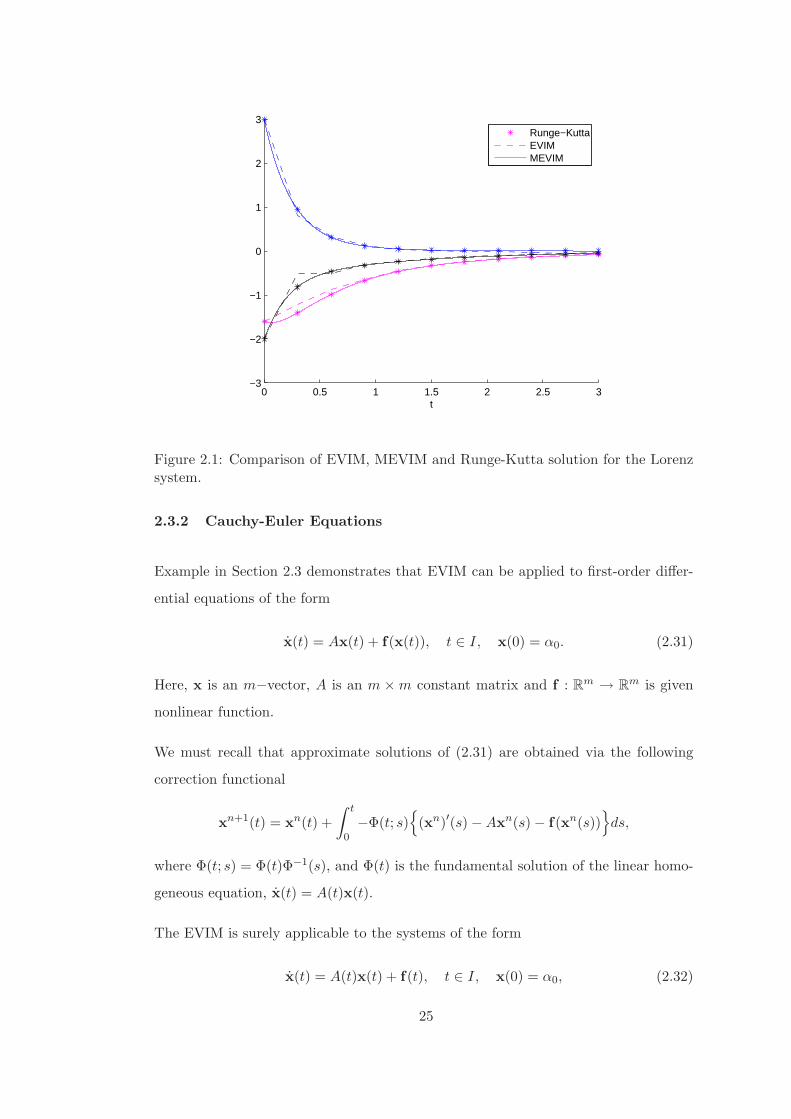
Figure 2.1 illustrates the results of Runge Kutta solution, EVIM, MEVIM for the fifth

order approximate solution. Further, we use the following notations in Table 2.1

εEV IMi (t) =

∣∣xEi (t) − xEV IM

i (t)∣∣ , εMEV IM

i (t) =∣∣xE

i (t) − xMEV IMi (t)

∣∣ ,

for i = 1, 2, 3, where xEi (t) denotes Runge-Kutta solution of xi and xEV IM

i (t), xMEV IMi (t),

denote the fifth-order approximate solutions of xi obtained by EVIM, MEVIM, respec-

tively.

Table 2.1: Comparison of the EVIM and MEVIM for the fifth-order approximationfor (2.26).

t εEV IM1

εMEV IM1

εEV IM2

εMEV IM2

εEV IM3

εMEV IM3

0 0 0 0 0 0 00.3 0.1882 0.0005 0.3152 0.0004 0.1382 0.00010.6 0.1064 0.0001 0.0494 0.0003 0.0229 0.00040.9 0.0342 0.0001 0.0061 0.0002 0.0003 0.00021.2 0.0178 0.0001 0.0110 0.0001 0.0060 0.00001.5 0.0092 0.0001 0.0161 0.0001 0.0125 0.00001.8 0.0075 0.0001 0.0181 0.0001 0.0160 0.00002.1 0.0095 0.0001 0.0185 0.0001 0.0215 0.00002.4 0.0122 0.0001 0.0172 0.0001 0.0344 0.00002.7 0.0143 0.0001 0.0099 0.0000 0.0574 0.0000

3 0.0333 0.0001 0.0208 0.0000 0.0762 0.0000

24

0 0.5 1 1.5 2 2.5 3−3

−2

−1

0

1

2

3

t

Runge−KuttaEVIMMEVIM

Figure 2.1: Comparison of EVIM, MEVIM and Runge-Kutta solution for the Lorenzsystem.

2.3.2 Cauchy-Euler Equations

Example in Section 2.3 demonstrates that EVIM can be applied to first-order differ-

ential equations of the form

x(t) = Ax(t) + f(x(t)), t ∈ I, x(0) = α0. (2.31)

Here, x is an m−vector, A is an m × m constant matrix and f : Rm → R

m is given

nonlinear function.

We must recall that approximate solutions of (2.31) are obtained via the following

correction functional

xn+1(t) = xn(t) +

∫ t

0−Φ(t; s)

(xn)′(s) − Axn(s) − f(xn(s))

ds,

where Φ(t; s) = Φ(t)Φ−1(s), and Φ(t) is the fundamental solution of the linear homo-

geneous equation, x(t) = A(t)x(t).

The EVIM is surely applicable to the systems of the form

x(t) = A(t)x(t) + f(t), t ∈ I, x(0) = α0, (2.32)

25

in particular. The difference between (2.31) and (2.32) is that in the former A is a

constant matrix while in the latter it is an m × m matrix of functions defined on I.

However, (2.32) is linear, but (2.31) is in general nonlinear.

In Chapter 2, it is seen that EVIM obtains the exact solution of x(t) = Ax(t) with only

a single iteration. This example shows that when the initial approximation satisfies

the initial condition then the first approximation obtained via EVIM is the exact

solution of (2.32). This fact will be proved in Theorem 2.6.

Consider the following Cauchy-Euler equation,

t2x − 3tx + 4x = t, t ∈ [1,∞), (2.33)

subject to the initial condition x(1) = 2, x(1) = 2. By using the transformation

x1 = x, x2 = x, equation (2.33) and the initial conditions can be rewritten as

x(t) = A(t)x(t) + f(t), x(1) = (2, 2)T , (2.34)

where

A(t) =

0 1

−4/t2 3/t

, f(t) =

0

1/t

.

The fundamental matrix Φ(t) of the homogeneous system x = A(t)x(t) is

Φ(t) =

t2 t2 ln(t)

2t 2t ln(t) + t

,

and hence, the solution of (2.34) is found to be

x(t) =(t2 − t2 ln(t) + t, t − 2t ln(t) + 1

)T.

Classical: For an approximate solution using VIM in literature so far, the following

correction functionals are used:

xn+11 (t) = xn

1 (t) +

∫ t

1λ1

(xn

1 )′(s) − xn2 (s)

ds,

xn+12 (t) = xn

2 (t) +

∫ t

1λ2

(xn

2 )′(s) +4xn

1 (s)

s2− 3xn

2 (s)

s+

1

s

ds.

(2.35)

Here, λ1 = λ1(s; t), λ2 = λ2(s; t) are the Lagrange multipliers and xn1 (s), xn

2 (s) are the

restricted variations and that δxn1 (1) = δxn

2 (1) = 0 holds for all n ∈ N.

26

The Lagrange multipliers considered in the classical approach are in general

λ1(s; t) = −1, λ2(s; t) = −1,

and the initial approximations for (2.35) are in general x01(t) = 2, x0

2(t) = 2.

Extended: Having generalised the Lagrange multipliers, the new approach used in

this thesis gives the following correction functional:

xn+1(t) = xn(t) +

∫ t

1ΛA(s; t)

(xn)′(s) − A(s)xn(s) − f(s)ds

,

where f(s) denotes the restricted variation, and the Lagrange multiplier, in this setting,

is given by

ΛA(s; t) = −

t2

s2

(1 − 2 ln

(t

s

))t2

sln

(t

s

)

−4t

s2ln

(t

s

)t

s

(1 + 2 ln

(t

s

))

.

Starting with the initial approximation x0(t) = (2, 2)T we immediately obtain the

exact solution

x1(t) =(t2 − t2 ln(t) + t, t − 2t ln(t) + 1

)T

of (2.34). Consequently, the solution x(t) of (2.33) is the first component of x1(t);

namely,

x(t) = t2 − t2 ln(t) + t.

Table 2.2 shows the absolute error of the fifth-order iteration obtained by the VIM

for t ∈ [1, 4]:

εV IMi (t) =

∣∣xEi (t) − xV IM

i (t)∣∣ ,

for i = 1, 2, where xV IMi (t) denotes the approximate solutions obtained by VIM for

the fifth-order iteration and xEi (t) denotes the exact solution obtained by EVIM at

the point t for i = 1, 2.

Furthermore, by

εV IM (t) =∥∥xE(t) − xV IM (t)

∥∥2,

we define the errors in the two-norm.

It must be noted that while EVIM obtains the exact solution at the single step,

however, error in VIM is accumulated when t gets relatively large.

27

Table 2.2: Comparison of the classical VIM and EVIM for the fifth-order approxima-tion for (2.34).

t εV IM1

εV IM2

εV IM

1 0 0 01.5 0.0002 0.0005 0.00062 0.0084 0.0105 0.0134

2.5 0.0626 0.0417 0.07523 0.2399 0.0914 0.2567

3.5 0.6468 0.1445 0.66284 1.4081 0.1802 1.4195

2.3.3 Bernoulli Equations

In Cauchy-Euler equation, we apply the method to the system of the form

x(t) = A(t)x(t) + f(t), t ∈ I, x(0) = α0. (2.36)

In general, the method is also applicable to the systems of the form

x(t) = A(t)x(t) + f(t,x(t)), t ∈ I, x(0) = α0. (2.37)

where f : I ×Rm −→ R

m is a given function, A is m×m matrix and x is an m-vector.

In this part, extended multistage variational iteration method is used for solving a

Bernoulli differential equation. The results are compared with the modified variational

iteration method for solving Riccati differential equations proposed by Geng [13].

Bernoulli equation is a first-order nonlinear differential equation of the form

x(t) + P (t)x(t) = Q(t)xq(t), x(0) = α0, (2.38)

where P and Q are continuous functions on I = [0, T ] and q 6∈ 0, 1. For this specific

example we let P (t) = Q(t) = t and q = 2 so that (2.38) takes the following form

x(t) + tx(t) = tx2(t), x(0) = α0 (2.39)

and the exact solution of which is easily found to be

x(t) =1

1 − et2/2(1 − 1/α0).

According to the extended multistage variational iteration method, we construct the

following correction functional

xn+1(t) = xn(t) +

∫ t

t∗λ

(xn)′(s) + sxn(s) − s(xn)2(s)

ds, (2.40)

28

where λ = λ(s; t) is the Lagrange multiplier, xn(s) is the restricted variation. The

initial approximation is x0(t) = α0. Here, the interval [0, T ] is divided into m + 1

subintervals, [t0, t1), [t1, t2),. . . , [tm, tm+1), with the convention that t0 = 0 and tm+1 =

T . In (2.40), t∗ is chosen to be the left boundary points of the subintervals, and within

each subinterval [t∗, tk) with 1 ≤ k ≤ m + 1, the initial approximate solution is xn(t∗)

which is obtained from the preceding subinterval or the initial condition x(0) = α0.

Either by using calculus of variations, but including all linear terms and that δxn(t∗) =

0, or directly from Theorem 2.1, we obtain

λ(s; t) = −e(s2−t2)/2.

Then, the Lagrange multiplier yields the following correction functional

xn+1(t) = xn(t) +

∫ t

t∗−e(s2−t2)/2

(xn)′(s) + sxn(s) − s(xn)2(s)

ds,

with the initial approximation x0(t) = α0.

In [13], Geng proposed a modification of VIM for equations of the type

x(t) = R(t) + P (t)x(t) + Q(t)x2(t), 0 ≤ t ≤ T,

x(0) = α(2.41)

where R(t), P (t), Q(t) are continuous functions in [0, T ]. Geng defined the following

iteration formula to solve the system (2.41)

xn+1(t) = xn(t) − γ

∫ t

0

(xn)′(s) − R(s) − P (s)xn(s) − Q(s)(xn)2(s)

ds,

for 0 ≤ t ≤ T , where x0(t) = α and |γ| is chosen to be relatively “small”, generally

less than unity [13].

In Table 2.3, we compare both methods for the system (2.41) for the fifth and the tenth

iterations with α0 = 1/2, T = 4 and γ = 0.001. It can be seen that the multistage

version of the new approach (MEVIM) is more effective than the method proposed

in [13], without the need for searching a (best) value for the artificial parameter γ.

One might have observed that the extended VIM can solve certain problems exactly in

one step. In fact, this is not a coincidence: the newly extended version of the method

solves linear equations in just a single step as long as the initial approximation satisfies

the initial condition. Of course, it cannot solve nonlinear ones within a single iteration.

29

Table 2.3: Comparison of the extended multistage variational iteration method and theproposed approach in [13] for γ = 0.001 for the fifth- and tenth-order approximations.

5th-order 10th-order

t Exact Error MEVIM Error VIM [13] Error MEVIM Error VIM [13]0 0.5000 0 0 0 0

0.5 0.4688 0.0000 0.0310 0.0000 0.03091 0.3775 0.0017 0.1218 0.0000 0.1212

1.5 0.2451 0.0267 0.2535 0.0043 0.25202 0.1192 0.0890 0.3782 0.0375 0.3757

2.5 0.0421 0.1431 0.4539 0.0811 0.45003 0.0110 0.1680 0.4833 0.1036 0.4776

3.5 0.0022 0.1756 0.4901 0.1106 0.48244 0.0003 0.1772 0.4896 0.1122 0.4795

Thus, before the convergence analysis of such a functional iteration scheme, we close

this section by stating and proving the theorem on that solution to linear systems can

be solved by a single step of the extended version of VIM.

Theorem 2.6. Consider the following linear initial value problem

x(t) = A(t)x(t) + f(t), x(0) = α0, t ∈ I := [0, ℓ], (2.42)

where x is an m-vector, A(t) = (aij(t)), aij ∈ C(I) is an m × m matrix. Let x0(t) ∈C1(I) such that x0(0) = α0 be a given initial approximation. Then, x1(t) defined by

the correction functional

x1(t) = x0(t) −∫ t

0Φ(t; s)

(x0)′(s) − A(s)x0(s) − f(s)

ds. (2.43)

is the exact solution of (2.42).

Proof. It is obvious that using the correction functional (2.43) we have

x1(0) = x0(0) = α0.

Upon calculating the derivative x1 as

x1(t) = x0(t) − Φ(t; t)

(x0)(t) − A(t)x0(t) − f(t)

−∫ t

0

∂

∂tΦ(t; s)

(xn)′(s) − A(s)xn(s) − f(s)

ds

and using the fact that∂Φ(t; s)

∂t= A(t)Φ(t; s),

Φ(t; t) = E,

30

we obtain

x1(t) = A(t)x0(t) + f(t) − A(t)

∫ t

0Φ(t; s)

(x0)′(s) − A(s)x0(s) − f(s)

ds.

Hence,

x1(t) = A(t)x1(t) + f(t)

completes the proof.

2.4 Convergence Analysis of EVIM

Variational iteration method has been used to approximate the solutions of different

problems. The method gives convergent successive approximations without using

neither linearisation nor perturbation techniques; and hence, the method reduces the

computational time in many applications.

The convergence of the method have been studied by researchers from different areas

and for different problems. For example; Torvattanabun and Koonprasert [55] studied

the convergence of the method for solving a first-order linear system of PDEs with

constant coefficients. Salkuyeh proposed a theorem for the convergence of the method

in solving linear system of ODEs with constant coefficients in [49]. Tatari and Dehghan

[54] investigated the sufficient conditions to prove the convergence of the method.

In [48], Ramos considered the first and second order time differentials and proved

that the iterative process of VIM can be obtained by using adjoint operators, Green’s

function, integration by parts and the method of weighted residuals. Ramos also

claimed that VIM is a specialised version of the Picard-Lindelof iterative process for

initial-value problems in ODE; the use of the Banach’s fixed point theory for initial-

value problems in PDE ensures the convergence of the method when the mapping is

Lipschitz continuous and contractive.

In this section of the present work we will investigate the conditions which guarantees

the convergence of EVIM and see the close relationship between the iterative process

obtained by EVIM and variations of parameters formula.

Now, let us consider the following system:

x = A(t)x(t) + f(t,x), t ∈ I := [0, ℓ] (2.44)

31

subject to the initial condition

x(0) = α0,

where x is an m−vector, A(t) = (aij(t)), aij ∈ C(I) is an m × m matrix and f :

I × Rm → R

m for m ∈ N.

Applying EVIM gives us the following iterative process:

xn+1(t) = xn(t) +

∫ t

0ΛA(s; t)

(xn)′(s) − A(s)xn(s) − f(s, xn(s))

ds, (2.45)

where xn(t) denotes the nth-order approximate solution and ΛA(s; t) is the m × m

matrix valued Lagrange multiplier. In Section 2.1, we have proved that

ΛA(s; t) = −Φ(t)Φ−1(s) = −Φ(t; s),

where Φ(t) denotes the fundamental matrix of the corresponding homogeneous differ-

ential equation x(t) = A(t)x(t).

Then, the correction functional (2.45) can be rewritten as follows

xn+1(t) = xn(t) −∫ t

0Φ(t; s)

(xn)′(s) − A(s)xn(s) − f(s,xn(s))

ds (2.46)

and the integration by parts yields

xn+1(t) = Φ(t; 0)xn(0) +

∫ t

0

Φ′(t; s)xn(s) + Φ(t; s)A(s)xn(s) + Φ(t; s)f(s,xn(s))

ds.

Hence, by using the fact that Φ′(t; s) = −Φ(t; s) A(s), we obtain

xn+1(t) = Φ(t; 0)xn(0) +

∫ t

0

Φ(t; s)f(s,xn(s))

ds. (2.47)

This formula is nothing else but the fixed point iteration for the variation of parameters

formula. However, f , in general, is a nonlinear function of the components of x.

Meanwhile, in the case when f is independent of x, but depends only on t, then

Theorem 2.6 becomes an obvious fact of (2.47).

To prove that the sequence xn∞n=1 converges to the exact solution of (2.44), we state

the following theorem.

Theorem 2.7. Let x(t) ∈ C1(I) for t ∈ I = [0, ℓ] be the exact solution of (2.44)

and xn(t) ∈ C1(I) be the nth order approximate solution obtained by the correction

functional (2.47) with x0(t) = α0, xn(0) = α0 for all n ∈ N. Let f ∈ (C(I), Lip); that

32

is f is a continuous function and it satisfies Lipschitz condition (with respect to x) in

I, with Lipschitz constant k > 0. Furthermore, ‖Φ(t; s)‖ ≤ F , and ‖f(s,x(s))‖ ≤ M

for all s ∈ I. Then, the sequence xn∞n=1 ∈ C1(I) converges uniformly to x.

Proof. It is a known fact that the unique solution of (2.44) has the following form

x(t) = Φ(t; 0)x(0) +

∫ t

0Φ(t; s)f(s,x(s))ds. (2.48)

The proof of the theorem is based on three steps. Firstly, we will find an error bound

for∥∥xn+1(t) − xn(t)

∥∥. Secondly, we will prove that xn(t) is a Cauchy sequence via

error bound obtained in the first step. Thirdly, we will show that xn(t) converges to

x(t).

Let n = 0, then the subtraction of first and zeroth approximation is

∥∥x1(t) − x0(t)∥∥ ≤ ‖(Φ(t; 0) − E)α0‖ +

∥∥∥∥∫ t

0Φ(t; s)f(s,x0(s))ds

∥∥∥∥ ,

where E denotes the m × m identity matrix. Since we have Φ(t; s) is bounded, the

(Φ(t; 0) − E) is also bounded, that is, ‖Φ(t; 0) − E‖ ≤ C. As a result, we obtain

∥∥x1(t) − x0(t)∥∥ ≤ C ‖α0‖ + FMt.

For n ≥ 0,

xn+1(t) − xn(t) = Φ(t; 0)xn(0) +

∫ t

0Φ(t; s)f(s,xn(s))ds

− Φ(t; 0)xn−1(0) −∫ t

0Φ(t; s)f(s,xn−1(s))ds

(2.49)

By using the fact that xn(0) = xn−1(0), we get

∥∥xn+1(t) − xn(t)∥∥ =

∥∥∥∥∫ t

0Φ(t; s)

(f(s,xn(s)) − f(s,xn−1(s))

)ds

∥∥∥∥

≤ Fk

∫ t

0

∥∥xn(s) − xn−1(s)∥∥ ds.

(2.50)

Now, iteratively we obtain

∥∥x2(t) − x1(t)∥∥ ≤ Fk

∫ t

0

∥∥x1(s) − x0(s)∥∥ ds ≤ Fk

(C ‖α0‖ t + FM

t2

2!

)

∥∥x3(t) − x2(t)∥∥ ≤ Fk

∫ t

0

∥∥x2(s) − x1(s)∥∥ ds ≤ (Fk)2

(C ‖α0‖

t2

2!+ FM

t3

3!

)

∥∥x4(t) − x3(t)∥∥ ≤ Fk

∫ t

0

∥∥x3(s) − x2(s)∥∥ ds ≤ (Fk)3

(C ‖α0‖

t3

3!+ FM

t4

4!

)

...∥∥xn+1(t) − xn(t)

∥∥ ≤ Fk

∫ t

0

∥∥xn(s) − xn−1(s)∥∥ ds ≤ (Fk)n

(C ‖α0‖

tn

n!+ FM

tn+1

(n + 1)!

).

(2.51)

33

Now, we obtain an error bound for∥∥xn+1(t) − xn(t)

∥∥, completing step one.

The second step is to show that xn(t) is a Cauchy sequence. Suppose that m < n,

‖xn(t) − xm(t)‖ =∥∥(

xn(t) − xn−1(t))

+(xn−1(t) − xn−2(t)

)+ . . . +

(xm+1(t) − xm(t)

)∥∥

≤n−1∑

j=m

∥∥xj+1(s) − xj(s)∥∥ ds

≤n−1∑

j=m

(Fk)j

(C ‖α0‖

tj

j!+ FM

tj+1

(j + 1)!

)

=n−1∑

j=m

(Fk)j

(C ‖α0‖

tj

j!

)+

n−1∑

j=m

(Fk)j

(FM

tj+1

(j + 1)!

)

These sums are parts of Taylor series for eFkt. By taking m sufficiently large it is

possible to make ‖xn(t) − xm(t)‖ less than any ǫ > 0. This shows that the sequence

xn(t) is Cauchy sequence.

Since xn(t) is a Cauchy sequence of continuous functions and I = [0, ℓ] is a compact

interval, then xn(t) converges uniformly to a continuous function x(t), that is

x(t) = limn→∞

xn+1(t)

= limn→∞

Φ(t; 0)xn(0) +

∫ t

0Φ(t; s)f(s,xn(s))ds

= Φ(t; 0)α0 + limn→∞

∫ t

0Φ(t; s)f(s,xn(s))ds

(2.52)

Now,

limn→∞

∫ t

0Φ(t; s)f(s,xn(s))ds =

∫ t

0Φ(t; s)f(s,x(s))ds

+

∫ t

0Φ(t; s) (f(s,xn(s)) − f(s,x(s))) ds.

(2.53)

Since xn(t) − x(t) converges uniformly to 0, then

∥∥∥∥∫ t

0Φ(t; s) (f(s,xn(s)) − f(s,x(s))) ds

∥∥∥∥ ≤ Fℓk ‖xn(s) − x(s)‖ −→ 0.

Finally,

limn→∞

xn+1(t) = Φ(t; 0)α0 +

∫ t

0Φ(t; s)f(s,x(s))ds.

which is the exact solution of (2.44).

For more details of the convergence properties of successive approximations, we re-

fer [8].

34

CHAPTER 3

SOLUTION OF INITIAL VALUE AND BOUNDARY

VALUE PROBLEMS BY THE VARIATIONAL

ITERATION METHOD

In this chapter of the present work, we will consider the mth order linear nonhomoge-

neous ordinary differential equations as well as nonlinear ones. We will mainly show

the existence of a close relation between the Lagrange multipliers and the adjoint

equations.

By using these relations, we will prove the basic properties of Lagrange multipliers

and show that it is also possible to obtain the solution of linear equations with only

a single variational iteration.

In the sequel, VIM represents the variational iteration method which does not use any

restricted variation while obtaining the scalar-valued Lagrange multiplier for an mth

order differential equations and EVIM represents the extended variational iteration

method which obtains the matrix-valued Lagrange multiplier for the corresponding

first-order differential equation.

3.1 Solution of Initial Value Problems

Let us consider the following higher order differential equation:

p0(t)x(m)(t) + p1(t)x

(m−1)(t) + p2(t)x(m−2)(t) + · · · + pm(t)x(t) = 0, (3.1)

35

for t ∈ I = [a, b] and subject to the initial conditions

x(a) = xa, x(a) = xa, x(2)(a) = x(2)a , . . . , x(m−1)(a) = x(m−1)

a ,

where pi ∈ Cm−i(I, R) , p0(t) > 0 for all t ∈ I, and x(i) represents the ith derivative

dix(t)/dti for all i = 1, 2, . . . , m.

Let Lm,t denotes the following differential operator:

Lm,t = p0(t)dm

dtm+ p1(t)

dm−1

dtm−1+ p2(t)

dm−2

dtm−2+ · · · + pm(t). (3.2)

By using the VIM, we can construct the following correction functional for equation

(3.1)

xn+1(t) = xn(t) +

∫ t

aλ

p0(s)x(m)n (s) + p1(s)x

(m−1)n (s)

+p2(s)x(m−2)n (s) + · · · + pm(s)xn(s)

ds.

(3.3)

Here, λ = λ(s; t) is the Lagrange multiplier, xn(t) represents the nth order approxi-

mate solution, and x(j)n (s) is the derivative djxn(s)/dsj for j = 1, 2, . . . , m.

By using integration by parts, it is easy to obtain the following equality [42]

∫ t

aλpm−r(s)x

(r)n (s)ds = λpm−r(s)x

(r−1)n (s) |s=t

s=a

−(λpm−r(s))′x

(r−2)n (s) |s=t

s=a + . . .

+(−1)r−1(λpm−r(s))(r−1)xn(s) |s=t

s=a

+(−1)r

∫ t

ax(s)(λpm−r(s))

(r)ds,

(3.4)

for all r = 1, 2, . . . , m. Taking the variation of both parts of the correction functional

yields

δxn+1(t) = δxn(t) + δ

∫ t

aλLm,sxn(s)ds

= δxn(t) +

∫ t

aλLm,sδxn(s)ds.

(3.5)

36

Using the equality in (3.4) and δxn(a) = 0, we obtain

δxn+1(t) =

(−1)m−1(λp0)(m−1) + (−1)m−2(λp1)

(m−2)

+ · · · + λpm−1 + 1

δxn(s)∣∣∣s=t

+

(−1)m−2(λp0)(m−2) + (−1)m−3(λp1)

(m−3)

+ · · · + λpm−2

δ(xn)′(s)

∣∣∣s=t

+

(−1)m−3(λp0)(m−3) + (−1)m−4(λp1)

(m−4)

+ · · · + λpm−3

δ(xn)′′(s)

∣∣∣s=t

...

+p0λδ(xn)(m−1)∣∣∣s=t

+

∫ t

aδxn(s)L†

m,sλds

where we have used λ = λ(s; t) and pi = pi(s) for all i = 0, 1, . . . , m − 1. Here, L†m,s

is given by

L†m,s(·) = (−1)m dm

dsm(p0(s)·) + (−1)m−1 dm−1

dsm−1(p1(s)·) + (−1)m−2 dm−2

dsm−2(p2(s)·)

+ · · · + (pm(s)·),

and hence,

L†m,sλ(s; t) = (−1)m(p0(s)λ(s; t))(m) + (−1)m−1(p1(s)λ(s; t))(m−1)

+(−1)m−2(p2(s)λ(s; t))(m−2) + · · · + pm(s)λ(s; t),

The operator L†m,s is called the adjoint of Lm,s in (3.2). Thus, the following conditions

makes the correction functionals stationary:

0 =

(−1)m−1(λ(s; t)p0(s))(m−1) + (−1)m−2(λ(s; t)p1(s))

(m−2)

+ · · · + λ(s; t)pm−1(s) + 1∣∣∣

s=t,

0 =

(−1)m−2(λ(s; t)p0(s))(m−2) + (−1)m−3(λ(s; t)p1(s))

(m−3)

+ · · · + λ(s; t)pm−2(s)∣∣∣

s=t,

0 =

(−1)m−3(λ(s; t)p0(s))(m−3) + (−1)m−4(λ(s; t)p1(s))

(m−4)

+ · · · + λ(s; t)pm−3(s)∣∣∣

s=t,

...

0 = p0(s)λ(s; t)∣∣∣s=t

,

(3.6)

Consequently, we have

L†m,sλ(s; t) = 0, (3.7)

37

and using the fact that λ(t, t) = 0, by backward substitution in (3.6), we obtain

∂jλ(s; t)

∂sj

∣∣∣s=t

= 0, forj = 0, 1, 2, . . . , m − 1,

∂m−1λ(s; t)

∂sm−1

∣∣∣s=t

=(−1)m

p0(t)

(3.8)

Without loss of generality we assume p0(t) = 1 and write

Lm,tx =dmx

dtm+ p1(t)

dm−1x

dtm−1+ p2(t)

dm−2x

dtm−2+ . . . + pm(t)x = 0, (3.9)

for which the associated system of first order equations is

x = A(t)x, (3.10)

where x = (x1, x2, . . . , xm)T = (x, x(2), . . . , x(m−1))T and A(t) is the companion matrix

with the following form:

A =

0 1 0 · · · 0

0 0 1 · · · 0...

......

. . . 1

−pm −pm−1 −pm−2 · · · −p1

. (3.11)

Initial conditions turn out to be

x(a) = (xa, xa, x(2)a , . . . , x(m−1)

a )T .

If we apply EVIM to system (3.10), we obtain the following functional

xn+1(t) = xn(t) +

∫ t

aΛ

(xn(s))′ − A(s)xn(s)

ds, (3.12)

where the Lagrange multiplier Λ = Λ(s; t) satisfies the following matrix differential

equation:

Λ′(s; t) = −Λ(s; t)A(s),

Λ(t; t) = −E.(3.13)

Here, we recall that ′ denotes the derivative with respect to s and ˙ denotes the

derivative with respect to t.

In Section 2.1, it is proven that the solution of (3.12) satisfies Λ(t; s) = −ΨT (t; s)

where Ψ(t) denotes the fundamental matrix of the adjoint equation

y = −AT (t)y, (3.14)

38

with

−AT =

0 0 · · · 0 pm

−1 0 · · · 0 pm−1

0 −1 · · · 0 pm−2

......

. . ....

...

0 0 · · · −1 p1

. (3.15)

The components of (3.14) give

y1 = pmym, yk = −yk−1 + pm−k+1ym, k = 2, 3, . . . , m,

by using (3.15). By differentiating the kth relation (k − 1) times we observe that ym

satisfies the adjoint differential equation

L†m,tym = (−1)m dm

dtmym + (−1)m−1 dm−1

dtm−1(p1ym)

+(−1)m−2 dm−2

dtm−2(p2ym) + · · · + pmym

= 0.

Since the Lagrange multiplier λ(s; t) of (3.3) will also satisfy L†m,sλ(s; t) = 0, it is

obvious that λ(s; t) and ym(t) solve the same differential equation but written with

respect to different variables: s and t, respectively.

If the fundamental solution of (3.14) is Ψ(t) then the components of the last row of

this matrix will be the linearly independent solutions of ym(t). By using this fact, we

can write

λ(t; s) = eTmΨ(t; s)c, (3.16)

where em = (0, 0, . . . , 1)T1×m and c = (c1, c2, . . . , cm)T where ci ∈ R for i = 1, 2, . . . , m.

By changing the roles of s and t we get

λ(s; t) = eTmΨ(s; t)c. (3.17)

Using the relation Ψ(s; t) = ΛT (s; t), we obtain the following relation for the Lagrange

multiplier of the VIM and that of the EVIM

λ(s; t) = eTmΛT (s; t)c. (3.18)

This result can be reduced to the following summation:

λ(s; t) =m∑

i=1

ciΛim(s; t), (3.19)

39

with Λ = (Λim) , 1 ≤ i ≤ m as the Lagrange multiplier. Using (3.13) we can write

Λ′ij(s; t) = −(Λi(j−1)(s; t) − pm−j+1Λim(s; t)), i, j = 1, 2, . . . , m, (3.20)

with Λi0 = 0. Equations (3.8) and (3.20) show that

c1 = 1, ci = 0, i = 2, 3, . . . , m.

Hence,

λ(s; t) = Λ1m(s; t).

Now, it is easy to find the derivatives of λ(s; t) with respect to t. Firstly, we remember

Λ(s; t) = −Φ(t; s) so that

Λ(s; t) = A(t)Λ(s; t),

Λ(s; s) = −E.(3.21)

This yields immediately that

Lm,tλ(s; t) = 0 (3.22)

holds. In fact, equation (3.20) gives the derivative of the components Λ(s; t) as follows

Λij(s; t) = Λ(i+1)j(s; t), Λmj(s; t) = −m∑

i=1

piΛ(m+1−i)j(s; t), Λjj(s; s) = −1.

By using the result λ(s; t) = Λ1m(s; t) and the derivative components of Λ(s; t), we

get

Lm,tλ(s; t) = 0,

subject to the initial conditions

∂jλ(s; t)

∂tj

∣∣∣t=s

= 0,∂m−1λ(s; t)

∂tm−1

∣∣∣t=s

= −1, j = 0, 1, . . . , m − 2.

Recall that we have obtained that Lagrange multiplier λ(s; t) satisfies adjoint equation

with respect to variable s; that is, L†m,sλ(s; t) = 0, and the values of the derivatives of

λ(s; t) with respect to s when s = t were given in (3.8).

By using the previous discussions, we can prove the following theorem which states

that if the initial approximation satisfies the initial condition then the solution of mth

order linear nonhomogenous ordinary differential equation can be obtained by a single

step of VIM. A similar result for EVIM was presented in Theorem 2.6.

40

Theorem 3.1. Let

Lm,tx =dmx

dtm+ p1(t)

dm−1x

dtm−1+ p2(t)

dm−2x

dtm−2+ · · · + pm(t)x = f(t) (3.23)

subject to the initial conditions

x(a) = xa, x(a) = xa, x(2)(a) = x(2)

a , . . . , x(m−1)(a) = x(m−1)a ,

where t ∈ I = [a, b], pi ∈ Cm−i(I, R), for all t ∈ I, and x(i) represents the derivative

dix(t)/dti for all i = 1, 2, . . . , m. Construct x0 ∈ C(I, R) which satisfies the initial

conditions. Then,

x1(t) = x0(t) +

∫ t

aλ(s; t)

Lm,sx0(s) − f(s)

ds

is the solution of (3.23).

Proof. By using the previous discussions, it is easy to prove that

x(j)1 (t) = x

(j)0 (t) +

∫ t

a

∂jλ(s; t)

∂tj

Lm,sx0(s) − f(s)

ds, j = 1, 2, . . . , m − 1,

and

x(m)1 (t) = x

(m)0 (t) +

∂m−1λ(s; t)

∂tm−1

∣∣∣s=t

Lm,tx0(t) − f(t)

+

∫ t

a

∂m−1λ(s; t)

∂tm−1

Lm,sx0(s) − f(s)

ds.

Hence,

Lm,tx1(t) = Lm,tx0(t) −

Lm,tx0(t) − f(t)

+

∫ t

aLm,tλ(s; t)

Lm,sx0(s) − f(s)

ds.

Since Lm,tλ(s; t) = 0 from (3.22), then we obtain

Lm,tx1(t) = f(t)

and also x(j)1 (a) = x

(j)0 (a) for j = 0, 1, . . . , m − 1. This completes the proof.

In order to illustrate the results of Theorem 3.1, we will consider the following example.

Example 3.2. Let us reconsider the following Cauchy-Euler differential equation

t2x − 3tx + 4x = t, with x(1) = 2, x(1) = 2. (3.24)

By dividing t2, equation (3.24) can be reduced to

x − 3

tx +

4

t2x =

1

t. (3.25)

41

In Section 2.3.2, this system is solved by EVIM and the Lagrange multiplier of the

extended version of the method is obtained as

ΛA(s; t) = −

t2

s2

(1 − 2 ln

(t

s

))t2

sln

(t

s

)

−4t

s2ln

(t

s

)t

s

(1 + 2 ln

(t

s

))

.

Classical VIM constructs the following recursive functional

xn+1(t) = xn(t) +

∫ t

1λ(s; t)

(xn)′′(s) − 3

s(xn)′(s) +

4

s2xn(s) − 1

s

ds.

By using the previous discussions, we obtain

λ(s; t) = Λ12(s; t) = − t2

sln

(t

s

).

It is also possible to obtain λ(s; t) via (3.7) and (3.8), that is

λ′′(s; t) +

(3λ(s; t)

s

)′

+4λ(s; t)

s2= 0,

λ(t; t) = 0,∂λ(s; t)

∂s

∣∣∣s=t

= 1,

(3.26)

which has the solution

λ(s; t) =−t2

sln

(t

s

).

Let x0(t) = 2t that satisfies x0(1) = 2, x0(1) = 2. Then,

x(t) = x1(t) = t − t2 ln t + t2

is the exact solution of (3.24).

3.2 Solutions of Linear Boundary Value Problems

In Section 3.1, the following type of problems are considered

Lm,tx = f(t), (3.27)

subject to the initial conditions

x(a) = xa, x(a) = xa, x(2)(a) = x(2)a , . . . , x(m−1)(a) = x(m−1)

a . (3.28)

It is proved that if the zeroth approximation of VIM satisfies the initial conditions

(3.28), then the first approximation of the VIM will be the (exact) solution of initial

value problem.

42

In this section, we will propose an algorithm for the following type of systems

Sx = f(t) (3.29)

where S is a differential operator generated by

Lm,tx = p0(t)x(m)(t) + p1(t)x

(m−1)(t) + p2(t)x(m−2)(t) + . . . + pm(t)x(t) (3.30)

and the boundary conditions

Uv(x) =m∑

j=1

Mvjx(j−1)(a) + Nvjx

(j−1)(b) = 0, v = 1, 2, . . . , m, (3.31)

where I = [a, b], a, b ∈ R, pj : I → R, and pj ∈ Cm−j(I, R) and f : I → R is a

continuous function.

Before launching into the new algorithm, we will state some basic theory of nonho-

mogenous boundary value problems of type (3.29). For the definitions and theorems

given in the section, we refer [8, 9, 42].

Using matrices and column vectors to analyse the system (3.31) will simplify the

discussions throughout the section. Let x denotes the column vector with components,

x, x, x(2), . . . , x(m−1). Namely,

x(t) = (x(t), x(t), x(2)(t), . . . , x(m−1)(t))T for t ∈ [a, b].

Then, the boundary conditions

Uv(x) =m∑

j=1

Mvjx(j−1)(a) + Nvjx

(j−1)(b) = 0, v = 1, 2, . . . , m, (3.32)

form the following system

U(x) = Mx(a) + Nx(b),

where U = (U1, U2, . . . , Um)T and M, N are m×m matrices with components Mvj , Nvj ,

respectively.

Unless stated otherwise, we assume that M, N forms a matrix with property that

rank(M : N) = m,

43

where (M : N) is defined by the matrix

(M : N) =

M11 · · · M1m N11 · · · N1m

.... . .

......

. . ....

Mm1 · · · Mmm Nm1 · · · Nmm

.

The former condition, rank(M : N) = m, implies that the homogeneous boundary

value problem

Lm,tx = 0, U(x) = 0,

has m linearly independent boundary conditions and hence, the problem has only

the trivial solution. In that case, the solution of nonhomogenous boundary value

problem (3.29) is determined by means of the Green’s function:

The Green’s function of the operator S is the function which has the following prop-

erties:

• G(t, s) is continuous and has continuous derivatives with respect to t up to order

(m − 2) inclusive for all values of t and s in the interval [a, b],

• For any fixed value of s in the interval (a, b) the function G(t, s) has continuous

derivatives of orders (m − 1) and m with respect to t in each of the intervals

[a, s) and (s, b]; the (m − 1)th derivative is discontinuous at t = s with a jump

of1

p0(s),

∂m−1G

∂tm−1(s + 0, s) − ∂m−1G

∂tm−1(s − 0, s) =

1

p0(s).

• In each of the intervals [a, s) and (s, b], G(t, s), considered as a function of t,

satisfies the function ℓ(G) = 0 and the boundary conditions Uv(G) = 0 for

v = 1, 2, . . . , m.

Theorem 3.3. If the boundary value problem Sx = 0 has only the trivial solution,

then the operator S has one and only one Green’s function.

Then, the solutions of systems (3.29) for any continuous function f(t), t ∈ I can be

obtained via following theorem.

44

Theorem 3.4. If the equation Sx = 0 has only the trivial solution, namely, x(t) = 0

for all t ∈ I, then for any function f(t) which is continuous in the interval I, then

there exists a solution of the equation Sx = f ; this solution is expressed by the formula

x(t) =

∫ b

aG(t, s)f(s)ds,

where G(t, s) denotes the Green’s function for the operator S.

We have seen that the solution of nonhomogenous boundary value problems (3.29)

can be obtained with Green’s function.

Now, using the results of Section 3.1, we will prove the following theorem for boundary

value problems (3.29). Following the theorem, we will propose an algorithm to obtain

the solution of boundary value problem (3.29) without any need of Green’s function,

by an example.

Theorem 3.5. Let

Sx = f(t) (3.33)

that is

Lm,tx =dmx

dtm+ p1(t)

dm−1x

dtm−1+ p2(t)

dm−2x

dtm−2+ . . . + pm(t)x = f(t),

subject to the boundary conditions

U(x) = 0,

where t ∈ I = [a, b], a, b ∈ R, f : I → R is a continuous function. Let x0 ∈ C(I, R)

which satisfies the boundary conditions. Then,

x1(t) = x1(t) − y1(t), (3.34)

will be the solution of (3.33). Here, x1(t) is the approximation obtained by the following

correction functional of VIM

x1(t) = x0(t) +

∫ t

aλ(s; t)

Lm,sx0(s) − f(s)

ds.

Moreover, y1 : I −→ R is a function satisfies the following equations

Lm,ty1 = 0,

U(y1) = U(x1).(3.35)

45

Proof. In previous section, it was shown that

Lm,tx1(t) = f(t).

Therefore,

Lm,t (x1 − y1) = Lm,t(x1) − Lm,t(y1) = f(t),

and

U (x1(t) − y1(t)) = U (x1(t)) − U (y1(t)) = 0.

Hence, the proof is completed.

This theorem shows that for systems of the type (3.33), it is possible to obtain the

solution of boundary value problem via a modified algorithm for the VIM. Moreover,

the proposed method does not need Green’s function [42].

In order to illustrate the results of the theorem and to forecast the basics of the

modified algorithm in the next section, we consider the following boundary value

problem

x + x = t2, with x(0) = 0, x(π) = 0 (3.36)

Let

x0(t) = cos(t) − 1

be the initial approximation that satisfies boundary conditions, namely x0(0) = 0,

x0(π) = 0. The VIM constructs the following approximation

x1(t) = x0(t) +

∫ t

0λ(s; t)

(x0)

′′(s) + x0(s) − s2

ds.

By using the previous discussions, we obtain the following equations for Lagrange

multiplier λ(s; t):

λ′′(s; t) + λ(s; t) = 0,

λ(t; t) = 0, λ′(s; t) |s=t = 1.(3.37)

Solving this gives

λ(s; t) = sin(s − t)

so that

x1(t) = cos(t) − 1 +

∫ t

0sin(s − t)

− 1 − s2

ds = 2 cos(t) + t2 − 2.

46

However,

x1(0) = 0, ˙x1(π) = 2π.

Thus, our aim is to find a function y1 that satisfies

y1 + y1 = 0, y1(0) = 0 and y1(π) = 2π.

This is an easy task, and

y1(t) = −2π sin(t)

will suffice. Consequently,

x1(t) = x(t) − y1(t) = 2 cos(t) + t2 − 2 + 2π sin(t)

is the exact solution of the boundary value problem in (3.36).

3.3 A New Algorithm for Boundary Value Problems

In the previous section, we analysed the nonhomogenous boundary value problems of

the type

Lm,tx = f(t), U(x) = 0, (3.38)

where t ∈ I = [a, b], a, b ∈ R, f : I → R is a continuous function. It is proved that

the solution of such systems can be expressed by an approximate solution of VIM and

a function determined by the boundary conditions.

In this section of the current work, we will propose an algorithm for the systems of

the following form

Lm,tx = f(t, x(t), x(t), x(2)(t), . . . , x(m−1)(t)), U(x) = 0, (3.39)

where t ∈ I and f is a continuous function with respect to all its components. Al-

though the theory of (linear) boundary value problems of the type (3.38) is widely

known, the corresponding theory of nonlinear systems, such as (3.39), has not been

studied as much. Herewith, we shall introduce a new approach for solving such non-

linear boundary value problems.

Now, let’s consider the following boundary value problem

Lm,ty = 0, U(y) = u (3.40)

47

where u is a given m-vector. Let φ1, φ2, . . . , φm be linearly independent solutions of

differential equation Lm,ty = 0 and Φ is the fundamental matrix for Lm,ty = 0 in the

following:

Φ = [φ1, φ2, . . . , φm] =

φ1 φ2 · · · φm

φ1 φ2 · · · φm

......

. . ....

φ(m−1)1 φ

(m−1)2 · · · φ

(m−1)m

.

Further, the boundary conditions of (3.39) can be extended as follows [9]:

U Φ = M Φ(a) + N Φ(b).

Before going back to the problem, finally, let us consider the solution of Lm,ty = 0 in

the form

y = c1φ1 + c2φ2 + · · · + cmφm,

where c1, c2, . . . , cm are parameters identified by boundary conditions U(y) = u.

By using the fundamental matrix, it is possible to write

U(y) = U Φc = u

where c is the column vector c = (c1, c2, . . . , cm)T . We must recall that we have m

linearly independent boundary conditions, that is, the nonsingularity of U Φ. Hence,

the unknown parameter c can be determined uniquely as

c = (U Φ)−1u.

Now, it is time to go back to our original problem (3.39). We will propose the new

algorithm to approximate the solutions of the (nonlinear) boundary value problems

in (3.39).

For systems (3.39), the VIM constructs the following correction functional

xn+1(t) = xn(t) +

∫ t

aλ

Lm,s(xn(s)) − f

ds, (3.41)

where λ = λ(s; t) is the Lagrange multiplier and

f = f(s, xn(s), (xn)′(s), (xn)′(2)(s), . . . , (xn)′(m−1)(s))

48

with x′(i) = dix/dsi for i = 1, 2, . . . , (m − 1). In our algorithm, we will modify

correction functional (3.41) as follows

xn+1(t) = xn(t) +

∫ t

aλLm,s(xn(s)) − f

ds. (3.42)

Here, xn shows the nth approximate solution that satisfies the boundary conditions

and xn+1 is the solution that does not necessarily satisfy the boundary conditions

U(x) = 0. So without loss of generality we assume

U(xn+1) = un+1.

By the preceding discussions it is possible to construct a function yn+1 so that

Lm,tyn+1 = 0, U(yn+1) = un+1.

Then, our proposed algorithm gives the (n + 1)th approximate solution as follows

xn+1(t) = xn+1(t) − yn+1(t).

It must be noted that

Lm,txn+1 = Lm,txn+1 − Lm,tyn+1 = f ,

U(xn+1) = U(xn+1) − U(yn+1) = 0.

where f = Lm,txn+1. Recursive application of the procedure for n = 0, 1, 2, . . . will

yield the result.

As an illustrative example of the algorithm, consider the following system

x = −(x)2 − 1 (3.43)

subject to the boundary conditions

x(0) = 0, x(1) = 0.

The exact solution of (3.43) subject to the boundary conditions is

x(t) = ln(cos(t) + tan(1) sin(t)).

Let x0 = 0 where x0(0) = 0, x0(1) = 0. The modified correction functional will give

x1 as follows:

x1(t) = x0(t) +

∫ t

0(s − t)

1ds,

= −t2/2

(3.44)

49

with x1(0) = 0, ˙x1(1) = −1. Clearly, φ1 = 1 and φ2 = t are the fundamental solutions

of y = 0. Therefore,

y1(t) = c0 + c1t

is also a solution of the homogeneous system y = 0 where c0, c1 are constants to be

determined from the relations y1(0) = 0 and y1(1) = −1. Hence, we obtain c0 = 0,

c1 = −1 and thus y1(t) = −t. So, the first variational iterate x1 turns to be

x1(t) = x1(t) − y1(t) = − t2

2+ t

that also satisfies the boundary conditions. Carrying out this recursive algorithm, we

approximate the solution to the boundary value problem.

Table 3.1 and Figure 3.1 show the approximate solutions xi(t) for i = 1, 3, 5, 7. There,

xE(t) denotes the exact solution at t. Namely, xE(t) = ln(cos(t) + tan(1) sin(t)). One

can see that the proposed method gets very close results to the exact solution at the

7th variational iterate.

Table 3.1: The results of the proposed algorithm for (3.43).

t x1(t) x3(t) x5(t) x7(t) xE(t)0 0 0 0 0 0

0.1 0.0950 0.1352 0.1399 0.1402 0.14020.2 0.1800 0.2472 0.2539 0.2542 0.25420.3 0.2550 0.3398 0.3472 0.3475 0.34750.4 0.3200 0.4156 0.4233 0.4236 0.42370.5 0.3750 0.4769 0.4847 0.4850 0.48500.6 0.4200 0.5253 0.5330 0.5333 0.53340.7 0.4550 0.5618 0.5695 0.5699 0.56990.8 0.4800 0.5873 0.5951 0.5954 0.59550.9 0.4950 0.6025 0.6102 0.6105 0.6106

1 0.5000 0.6075 0.6152 0.6155 0.6156

50

0 0.2 0.4 0.6 0.8 10

0.1

0.2

0.3

0.4

0.5

0.6

0.7

x1(t)

x3(t)

x5(t)

x7(t)

xE(t)

Figure 3.1: Comparison of the approximate solutions obtained by the proposed algo-rithm and the exact solution of (3.43).

51

CHAPTER 4

APPLICATIONS

In this chapter, we implement the variational iteration method to solve various types

of problems. In the first section, we will apply the method to linear Sturm-Liouville

eigenvalue problems. In the second section, we will apply the method to Brusselator

model, and in the third one, we will use the method to solve the Chemical Master

Equation (CME).

4.1 Variational Iteration Method for Sturm-Liouville Differential Equa-

tions

A linear Sturm-Liouville operator has the form,

Tx(t) := Lx(t) = λr(t)x(t), (4.1)

where L = − d

dt

[p(t)

d

dt

]+ q(t), t ∈ I := [a, b]. Associated with the differential

equation (4.1) are the separated homogeneous boundary conditions

α1x(a) + β1x(a) = 0,

α2x(b) + β2x(b) = 0,

where α1, α2, β1 and β2 are arbitrary constants provided that α2i +β2

i 6= 0 for i = 1, 2.

The values of λ for which the boundary value problem has a nontrivial solution are

called eigenvalues of L. A nontrivial solution corresponding to an eigenvalue is called

an eigenfunction. We will assume that p(t), p(t), q(t) and r(t) are continuous functions

such that p(t) > 0 and r(t) > 0 for all t ∈ I [8, 53], for simplicity.

52

The main objective of this section is to implement VIM for computing eigenvalues of

Sturm-Liouville problems.

Example 4.1. Consider the Sturm-Liouville system

−x(t) − λx(t) = 0, t ∈ I = (−ℓ, ℓ), ℓ > 0, (4.2)

with homogeneous boundary conditions

x(−ℓ) = 0, x(ℓ) = 0. (4.3)

The correction functional of differential equation (4.2) has the following form:

xn+1(t, λ) = xn(t, λ) +

∫ t

−ℓµ− x′′

n(s, λ) − λxn(s, λ)

ds, (4.4)

where µ = µ(s; t, λ) is the Lagrange multiplier [26, 30]. Then, we have

δxn+1(t, λ) = δxn(t, λ) + δ

∫ t

−ℓµ (s; t, λ)

− x′′

n(s, λ) − λxn(s, λ)

ds.

Note that δxn(−ℓ, λ) = 0. Calculus of variations and integration by parts give the

stationary conditions

µ′′(s; t, λ) + λµ(s; t, λ) = 0,

1 + µ′(s; t, λ) |s=t = 0,

µ (s; t, λ) |s=t = 0,

for which the Lagrange multiplier µ should satisfy. Solving this system of equations

for µ yields

µ(s; t, λ) = − 1√λ

sin(√

λ(s − t)).

Thus, by inserting the Lagrange multiplier into (4.4) we obtain

xn+1(t, λ) = xn(t, λ)

+

∫ t

−ℓ− 1√

λsin(

√λ(s − t))

− x′′

n(s, λ) − λxn(s, λ)

ds. (4.5)

As an initial approximating solution, let us choose

x0(t, λ) = A + Bt,

where A and B are constants that are going to be defined by imposing the boundary

conditions (4.3) on the iterates and normalisation of the corresponding eigenfunctions.

Substituting x0(t, λ) in (4.5) gives

x1(t, λ) = A cos(√

λt) +B√λ

sin(√

λt).

53

If the function x1(t, λ) is now forced to satisfy the boundary conditions at t = −ℓ and

t = ℓ, then we get

x1(−ℓ, λ) = A cos(√

λℓ) − B√λ

sin(√

λℓ) = 0,

x1(ℓ, λ) = A cos(√

λℓ) +B√λ

sin(√

λℓ) = 0.

In order to have a nontrivial solution x1(t, λ), the system yields two infinite sequences

of eigenvalues λn,

λn =

((2n + 1)π

2ℓ

)2

, n = 0, 1, 2, . . . ,

λn =(nπ

ℓ

)2, n = 1, 2, . . . .

The corresponding linearly independent eigenfunctions un and vn are

un(t) = A cos

((2n + 1)π

2ℓt

), n = 0, 1, 2, . . . ,

vn(t) = Bℓ

nπsin

(nπ

ℓt)

, n = 1, 2, . . . .

Here un(t), vn(t) ∈ C(I, R); that is un(t) and vn(t) are continuous real valued functions

on I = (−ℓ, ℓ). The usual inner product on C(I, R) is defined by

〈un, vn〉 =

∫ ℓ

−ℓun(s)vn(s)ds, un, vn ∈ C(I, R),

and the norm induced by the inner product is

‖un‖2 = 〈un, un〉12 =

(∫ ℓ

−ℓ|un(s)|2ds

) 12

.

Consequently, we obtain

A =1√ℓ, B =

nπ

ℓ32

.

Therefore, the normalised eigenfunctions tn(t) =un(t)

‖un‖2and zn(t) =

vn(t)

‖vn‖2have the

forms

tn(t) =1√ℓ

cos(√

λnt)

with λn =

((2n + 1)π

2ℓ

)2

, n = 0, 1, 2, . . . ,

zn(t) =1√ℓ

sin(√

λnt)

with λn =(nπ

ℓ

)2, n = 1, 2, . . . .

These eigenvalues and eigenfunctions are the exact eigen-pairs of the Sturm-Liouville

system in (4.2).

54

Example 4.2. As another example consider the eigenvalue problem

−x(t) − λx(t) = 0, t ∈ I = (−ℓ, ℓ), ℓ > 0, (4.6)

with Neumann boundary conditions,

x(−ℓ) = 0, x(ℓ) = 0. (4.7)

Using variational iteration method, we can construct the correction functional of (4.6)

as follows:

xn+1(t, λ) = xn(t, λ)

+

∫ t

−ℓµ− x′′

n(s, λ) − λxn(s, λ)

ds, (4.8)

where µ = µ (s; t, λ) is the Lagrange multiplier. Note that δxn(−ℓ, λ) = 0.

The Lagrange multiplier can be identified as

µ(s; t, λ) = − 1√λ

sin(√

λ(s − t)),

so that the iterations in (4.8) can be written as follows:

xn+1(t, λ) = xn(t, λ)

+

∫ t

−ℓ− 1√

λsin(

√λ(s − t))

− x′′

n(s, λ) − λxn(s, λ)

ds. (4.9)

We begin with an initial approximation x0(t, λ) = A+Bt where A and B are constants

to be determined as before. By the correction functional (4.9), we get

x1(t, λ) = A cos(√

λt) +B√λ

sin(√

λt). (4.10)

Then,

x′1(−ℓ, λ) = A

√λ sin(

√λℓ) + B cos(

√λℓ) = 0,

x′1(ℓ, λ) = −A

√λ sin(

√λℓ) + B cos(

√λℓ) = 0.

Thus, the eigenvalues of this system have the form

λn =

((2n + 1)π

2ℓ

)2

, n = 0, 1, 2, . . .

λn =(nπ

ℓ

)2, n = 1, 2, . . . .

55

Corresponding linearly independent nontrivial solutions are

un(t) = B2ℓ

(2n + 1)πsin

(√λnt

)with λn =

((2n + 1)π

2ℓ

)2

, n = 0, 1, 2, . . . ,

vn(t) = A cos(√

λnt)

with λn =(nπ

ℓ

)2, n = 1, 2, . . . .

So, the normalisation constants are

A =1√ℓ, B =

(2n + 1)π

2ℓ32

.

Let tn(t) =un(t)

‖un‖2and zn(t) =

vn(t)

‖vn‖2, then

tn(t) =1√ℓ

sin

((2n + 1)π

2ℓt

)n = 0, 1, 2, . . . ,

zn(t) =1√ℓ

cos(nπ

ℓt)

, n = 1, 2, . . . .

Example 4.3. Now consider the following equation [53],

−x(t) + (t2 − λ)x(t) = 0, t ∈ I = (−∞,∞). (4.11)

The solutions of the system (4.11) are in the following form

x∞n = Ane−t2/2Hn(t), λ∞

n = 2n + 1, n = 0, 1 . . . .

where Hn(x) denotes the Hermite polynomials and An are normalisation constants

[53].

Let us consider system (4.11) in a truncated domain, −ℓ ≤ t ≤ ℓ for all ℓ > 0. The

new system is,

−x + (t2 − λ)x(t) = 0, (4.12)

with Dirichlet boundary conditions x(−ℓ) = 0, x(ℓ) = 0. To find the approximate

solution of equation (4.12) by means of variational method, the following correction

functional can be constructed as

xn+1(t, λ) = xn(t, λ)

+

∫ t

−ℓµ− x′′

n(s, λ) + s2xn(s, λ) − λxn(s, λ)

ds,

where µ = µ(s; t, λ) is the Lagrange multiplier and xn denotes restricted variation that

is δxn = 0. Following the discussions presented in the previous examples, we obtain

56

the iteration formula

xn+1(t, λ) = xn(t, λ)

+

∫ t

−ℓ− 1√

λsin(

√λ(s − t))

− x′′

n(s, λ) + s2xn(s, λ) − λyn(s, λ)

ds.

Let us start again with an initial approximation x0(t, λ) = A + Bt, where A and B

are real unknown constants. Then,

x1(t, λ) = A + Bt

+

∫ t

−ℓ− 1√

λsin(

√λ(s − t))

s2(A + Bs) − λ(A + Bs)

ds.

In Table 4.1, we present the eigenvalues of system (4.12) for different values of ℓ and

they are compared with the exact values λ∞n = 2n + 1 for n = 0, 1 . . ..

Table 4.1: Eigenvalues of equation (4.12) obtained by the variational iteration methodfor ℓ = 2, π and 4.5.

n ℓ Number of iterations λ |λ − λ∞n| λ∞

n

0 2 3 1.0823 0.0823 15 1.0749 0.07506 1.0749 0.07497 1.0749 0.0749

π 3 1.3952 0.3952 15 1.0177 0.01776 1.0030 0.00307 1.0006 0.0006

4.5 3 NaN 15 NaN6 1.2771 0.27717 1.1007 0.1007

1 2 3 1.0823 1.9177 35 1.9177 1.92516 1.0749 1.92517 1.0749 1.9251

π 3 3.1665 0.1665 35 4.8576 1.85766 1.0030 1.99707 1.0030 1.9970

4.5 3 NaN 35 NaN6 3.2916 0.29167 4.0764 1.0764

57

4.2 Variational Iteration Method for Brusselator Reaction-Diffusion

System

In this section of the present work, we will investigate the dynamical behaviour of

Brusselator reaction system which was proposed by Prigogine and Lefever as a model

for chemical dynamics [47]. The mechanism of Brusselator system is as follows [3,35,

44,47,58,61]

A −→ X, (4.13a)

B + X −→ Y + D, (4.13b)

2X + Y −→ 3X, (4.13c)

X −→ E. (4.13d)

Here, A and B denote the input chemicals, D and E are output chemicals and X, Y

are intermediates. It is a known fact that the reaction step (4.13c) can be observed in

the formation of ozone by atomic oxygen, inenzymatic reactions, in plasma and laser

physics [3, 57, 61]. The differential equations associated with (4.13) are given [47]:

∂X

∂t= c1A − c2BX + c3X

2Y − c4Dx∇2X

∂Y

∂t= c2BX − c3X

2Y Dy∇2Y,(4.14)

where c1, c2, c3, c4 denote the reaction constants of (4.13a), (4.13b), (4.13c), (4.13d),

respectively.

Let u = u(x, y, t) and v = v(x, y, t) denote the concentration of products at time

t, A, B are the constant concentrations of two input chemicals and α is a constant

represents Dx, Dy and L is the reactor length.

Then, the partial differential equations that represents the Brusselator model is as

follows [3, 57]:

∂u

∂t= A + u2v − (B + 1)u + α

(∂2u

∂x2+

∂2u

∂y2

),

∂v

∂t= Bu − u2v + α

(∂2v

∂x2+

∂2v

∂y2

),

(4.15)

for 0 < x, y < L, 0 < t < T . Then, we impose the Dirichlet boundary conditions of

58

the following type:

u(t, x, 0) = 0, v(t, x, 0) = 0, for 0 < x < L, 0 < t < T,

u(t, x, 1) = 0, v(t, x, 1) = 0, for 0 < x < L, 0 < t < T,

u(t, 0, y) = 0, v(t, 0, y) = 0, for 0 < y < L, 0 < t < T,

u(t, 1, y) = 0, v(t, 1, y) = 0, for 0 < y < L, 0 < t < T,

(4.16)

and initial conditions

u(0, x, y) = x, v(0, x, y) = xy2 0 < x, y < L. (4.17)

Semi-discrete methods which discretise in space and leave time variable continuous is

a way to approximate solutions of system (4.15).

Let the discretisation of the domain be such that xi = i∆x, yj = j∆y, i = 0, 1,. . .,n+1,

j = 0, 1, . . . , m + 1 with ∆x =1

n + 1, ∆y =

1

m + 1. Then, the second derivatives

uxx, uyy and vxx, vyy can be replaced, respectively, with the following differences:

uxx(t, xi, yj) ≈ u(t, xi+1, yj) − 2u(t, xi, yj) + u(t, xi−1, yj)

(∆x)2,

vxx(t, xi, yj) ≈ v(t, xi+1, yj) − 2v(t, xi, yj) + v(t, xi−1, yj)

(∆x)2,

and

uyy(t, xi, yj) ≈ u(t, xi, yj+1) − 2u(t, xi, yj) + u(t, xi, yj−1)

(∆y)2,

vyy(t, xi, yj) ≈ v(t, xi, yj+1) − 2v(t, xi, yj) + v(t, xi, yj−1)

(∆y)2,

for i = 1, 2, . . . , n and j = 1, 2, . . . , m.

Let ui,j and vi,j denote the u(t, xi, yj) and v(t, xi, yj), respectively. It is possible to

obtain a system of ODEs at mesh points xi, yj for i = 1, 2, . . . , n, j = 1, 2, . . . , m; such

as,

ui,j = A + u2i,jvi,j − (B + 1)ui,j

+ α

(ui+1,j − 2ui,j + ui−1,j

(∆x)2+

ui,j+1 − 2ui,j + ui,j−1

(∆y)2

),

vi,j = Bui,j − u2i,jvi,j

+ α

(vi+1,j − 2vi,j + vi−1,j

(∆x)2+

vi,j+1 − 2vi,j + vi,j−1

(∆y)2

).

(4.18)

Here,ui,j , vi,j denote dui,j/dt, dvi,j/dt. From boundary conditions we know that

ui,0 = 0, vi,0 = 0, i = 0, 1, . . . , n + 1,

ui,m+1 = 0, vi,m+1 = 0, i = 0, 1, . . . , n + 1,

u0,j = 0, v0,j = 0, j = 0, 1, . . . , m + 1,

un+1,j = 0, vn+1,j = 0, j = 0, 1, . . . , m + 1.

(4.19)

59

and the initial conditions

u(0, xi, yj) = xi, i = 1, 2, . . . , n, j = 1, 2, . . . , m,

v(0, xi, yj) = xiy2j , i = 1, 2, . . . , n, j = 1, 2, . . . , m.

(4.20)

To simplify the notation, let us write the system (4.18) as follows:

z = Sz + f(z), (4.21)

where z = (ui,j , vi,j),

S =

−(B + 1) − 2α

(∆x)2− 2α

(∆y)20

B − 2α

(∆x)2− 2α

(∆y)2

,

and

f(z) =

α

(ui+1,j + ui−1,j

(∆x)2+

ui,j+1 + ui,j−1

(∆y)2

)+ A + u2

i,jvi,j

α

(vi+1,j + vi−1,j

(∆x)2+

vi,j+1 + vi,j−1

(∆y)2

)− u2

i,jvi,j

.

Let, now, A = 0.5, B = 1, α = 1/64, ∆x = 0.25, ∆y = 0.25, L = 1 and T = 1 so that

(4.21) can be rewritten as

z =

−3 0

1 −1

z +

0.25 (ui+1,j + ui−1,j + ui,j+1 + ui,j−1) + 0.5 + u2

i,jvi,j

0.25 (vi+1,j + vi−1,j + vi,j+1 + vi,j−1) − u2i,jvi,j

.

Transforming the variable z to w by setting w = Pz, we obtain a diagonalised system

in w as

w = Jw + P−1f(Pz), (4.22)

where

P =

0 0.89

1 −0.45

, P−1 =

0.5 1

1.12 0

, and J =

−1 0

0 −3

.

Correction functional of the transformed system is

wn+1(t) = wn(s) +

∫ t

0ΛJ(s, t)

(wn)′(s) − Jwn(s) + P−1f(wn(s))

for t ∈ [0, 1], and with wn(s) being the restricted variation. It must be noted that

initial conditions (4.20) and boundary conditions (4.19) are transformed to the new

60

variable w, and initial condition of new variable is used as the zeroth approximate

solution. The Lagrange multiplier ΛJ(s, t) is

ΛJ(s, t) = −e−J(s−t) =

−e(s−t) 0

0 −e3(s−t)

.

If we divide [0, 1] time interval into subintervals [0, t1), [t1, t2), . . . , [t9, 1) where ti = i∆ℓ

with ∆ℓ = 0.1, for every i = 1, 2, . . . , 9, then we can construct the following correction

functional of MEVIM:

wn+1(t) = wn(s) +

∫ t

t∗−e−J(s−t)

(wn)′(s) − Jwn(s) + P−1f(wn(s))

,

where t∗ ∈ 0, t1, t2, . . . , t9 and

w(t∗) = wn(t∗), (4.23)

where w at the right hand-side of (4.23) denotes the nth order approximate solution

in [tk, t∗) where k ∈ 0, 1, . . . , t9.

In Table 4.2, we compare the fifth order approximate solutions of MEVIM and EVIM

with results obtained by Runge-Kutta methods for solving system (4.18). We use the

notation

εEV IMui,j

(t) =∣∣uEV IM

i,j (t) − uEi,j(t)

∣∣ , εMEV IMui,j

(t) =∣∣uMEV IM

i,j (t) − uEi,j(t)

∣∣ ,

εEV IMvi,j

(t) =∣∣vEV IM

i,j (t) − vEi,j(t)

∣∣ , εMEV IMvi,j

(t) =∣∣vMEV IM

i,j (t) − vEi,j(t)

∣∣ .

Here, uEV IMi,j (t), uMEV IM

i,j (t), uEi,j(t) denote the approximate solutions of u at points

xi, yj , t obtained by EVIM, MEVIM, and Runge-Kutta, respectively. Similarly,

vEV IMi,j (t), vMEV IM

i,j (t), and vEi,j(t) denote the approximate solutions of v at points

xi, yj , t obtained by EVIM, MEVIM and Runge-Kutta, respectively.

Now, let us consider the Brusselator system (4.15) with α = 0 so that we have an

ODE case. Then, we get the following system

u = A − (B + 1)u + u2v,

v = Bu − u2v,(4.24)

where u and v denote the concentrations of two reactants at time t and a, b ∈ R with

A, B > 0. It is easy to observe that (u∗, v∗) = (A, BA ) is an equilibrium point of the

61

Table 4.2: Absolute errors for the fifth-order approximation of EVIM and MEVIM.

t εEV IMu2,2

εMEV IMu2,2

εEV IMv4,4

εMEV IMv4,4

0 0 0 0 00.1 0.0198 0.0202 0.7727 0.82320.2 0.0320 0.0327 0.5856 0.24070.3 0.0379 0.0261 0.1699 0.14880.4 0.0392 0.0138 0.2272 0.03640.5 0.0370 0.0110 0.5621 0.18460.6 0.0325 0.0104 0.8188 0.02680.7 0.0266 0.0062 0.9857 0.12510.8 0.0200 0.0043 1.0656 0.15980.9 0.0132 0.0042 1.0731 0.19091 0.0065 0.0022 1.0228 0.1705

system. It is known that when 1 − B + A2 ≥ 0, the equilibrium point is a stable

one [57].

Classical: Let us suppose that A = 3 and B = 1, so that the equilibrium point is

stable; and let (u(0), v(0))T = (1, 2)T be the initial state of the system. To find the

approximate solution of system (4.24) by means of variational iteration method, we

can construct the following correction functionals

un+1(t) = un(t) +

∫ t

0µ1

(un)′(s) + 2u(s) − (un(s))2vn(s) − 3

ds,

vn+1(t) = vn(t) +

∫ t

0µ2

(vn)′(s) − un(s) + (un(s))2vn(s)

ds,

where µ1 = µ1(s; t), µ2 = µ2(s; t) are the general Lagrange multipliers and un(s) and

vn(s) are restricted variations, i.e., δun(s) = δvn(s) = 0. We therefore calculate the

Lagrange multipliers as

µ1(s; t) = −e2(s−t), µ2(s; t) = −1.

By substituting the multipliers into the correction functionals, we obtain the following

formulae for the approximate solutions:

un+1(t) = un(t) +

∫ t

0(−e2(s−t))

(un)′(s) + 2u(s) − (un(s))2vn(s) − 3

ds,

vn+1(t) = vn(t) +

∫ t

0(−1)

(vn)′(s) − un(s) + (un(s))2vn(s)

ds,

with initial approximations u0(t) = 1 and v0(t) = 2.

Extended: Using matrices and vectors, x = (u, v)T , system (4.24) can be rewritten

62

as follows

x = Mx + f(t,x), x(0) = (1, 2)T , (4.25)

where

M =

−2 0

1 0

and f(t,x) =

3 + x2

1x2

−x21x2

.

It must be noted that same as the classical VIM, we choose a = 1 and b = 3. Setting

x = Py, the transformed equation turns to be

y = Jy + f(t,y) =

0 0

0 −2

y1

y2

+

3/2 − 2y2

2(y1 − y2)

3/2 + 2y22(y1 − y2)

, (4.26)

together with the initial value

y(0) = (5/2, 1/2)T ,

where P =

0 2

1 −1

and P−1 =

1/2 1

1/2 0

. The correction functional of sys-

tem (4.26) can be written as

yn+1(t) = yn(t) +

∫ t

0ΛJ(s; t)

(yn)′(s) − Jyn(s) − f(s, yn(s))

ds,

with initial approximation y0(t) = y(0), where yn(s) denotes the restricted variation

vector. Hence, we obtain the Lagrange multiplier ΛJ(s; t) as

ΛJ(s, t) = −

1 0

0 e2(s−t)

.

Then, by using the transformation x = Py one can construct an approximate solution

of original system (4.25).

Table 4.3 shows the absolute errors of the nth order approximations obtained from

the application of the classical and the extended approach. Henceforth, we define

εV IMi =

∣∣xV IMi − xE

i

∣∣ , εEV IMi =

∣∣xEV IMi − xE

i

∣∣ , i = 1, 2,

where xEi is the Runge-Kutta solution, and xV IM

i and xEV IMi are the solutions ob-

tained by VIM and EVIM at t = 0.5, respectively.

Figure 4.1 illustrates a comparison between the two approaches for the tenth-order

approximation.

63

Table 4.3: Comparison of the classical and the proposed approach to VIM for theBrusselator system at point t = 0.5.

n εV IM1

εEV IM1

εV IM2

εEV IM2

1 0.969744 0.969744 0.899420 1.1753302 0.171587 0.045379 0.062814 0.0788163 0.034040 0.046744 0.004173 0.0465314 0.011708 0.008104 0.006337 0.0085725 0.001194 0.001062 0.000142 0.0010556 0.000402 0.000083 0.000199 0.0000877 0.000042 0.000006 0.000004 0.0000068 0.000008 0.000000 0.000003 0.0000009 0.000001 0.000000 0.000000 0.00000010 0.000000 0.000000 0.000000 0.000000

In the previous applications, we have applied EVIM to the differential systems of the

form

x(t) = Ax(t) + f(t,x(t)), t ∈ I, x(0) = α0.

where A is 2×2 matrix, f : I×R2 → R

2 is a given nonlinear function and x is 2-vector.

In the next example, we will illustrate that EVIM and MEVIM is more suitable than

the classical VIM and MVIM for systems where A is an n×n matrix, where n is larger

than 2.

To prove the efficiency of the method for such systems, we will use the Brusselator

model which was proposed by Tyson [58] in 1972. This system is constructed by using

two Brusselators. In this model the outputs of the first Brusselator model are used as

the inputs of the second one. The reactions of the new models are given by [61]:

A −→ X, B + X −→ Y + D, 2X + Y −→ 3X, X −→ E,

D + E −→ F + G, 2E + F −→ 3H, H −→ K.(4.27)

The differential equation associated by (4.27) are [58,61]

z1 = f1(z, A, B) = A − Bz1 + (z1)2z2 − z1,

z2 = f2(z, A, B) = Bz1 − (z1)2z2,

z3 = f3(z, A, B) = z1 − z3z4,

z4 = f4(z, A, B) = Bz1 − z3z4 + (z4)2z5 − z4,

z5 = f5(z, A, B) = z3z4 − (z4)2z5,

(4.28)

where z = (z1, z2, z3, z4, z5)T = (X, Y, D, H, F )T , A and B are real constants and

64

2.9179 2.9179 2.9179 2.9179 2.9179 2.9179 2.9179 2.9179 2.9179

0.6006

0.6006

0.6006

0.6006

0.6006

0.6006

u

v

ExactVIMEVIM

Figure 4.1: Comparison between the classical and the proposed approach to VIM forthe tenth-order approximation.

t ∈ [0, T ], T > 0. Let A = 1, B = 0.5. Then, (4.28) can be written

z = Mz + f(z) (4.29)

where

M =

−1.5 0 0 0 0

0.5 0 0 0 0

1 0 0 0 0

0.5 0 0 −1 0

0 0 0 0 0

and f(z) =

(z1)2z2 + 1

−(z1)2z2

−(z3)z4

−z3z4 + (z4)2z5

z3z4 − (z4)2z5

.

Let us impose the initial conditions to be

z(0) = (0.8, 0.4, 1.8, 0.4, 3.75)T .

Since the matrix A is a constant matrix, it is possible to introduce w = Pz transfor-

65

mation where

P =

0 0 0 0.6255 0

1 1 0 −0.2085 0

0 0 1 −0.4170 0

1 0 0 −0.6255 0

0 0 0 0 1

.

Then, (4.29) is transformed to

w = Jw + f(w), (4.30)

with w(0) = (1.2000, 0.6667, 2.3333, 1.2789, 3.7500)T . To obtain the approximate so-

lutions of system (4.30) by means of EVIM, the following correction functional will

be constructed

wn+1(t) = wn(s) +

∫ t

0−e−J(s−t)

(wn)′(s) − Jwn(s) + f(wn(s))

(4.31)

for t ∈ [0, 1]. If we want to apply MEVIM, correction functional (4.31) takes the

following form,

wn+1(t) = wn(s) +

∫ t

t∗−e−J(s−t)

(wn)′(s) − Jwn(s)f(wn(s))

(4.32)

where t∗ ∈ t1, t2, . . . , tn where [0, 1) = [0, t1) ∪ [t1, t2) . . . [tn, 1). It must be noted

that for both cases w0 = w(0) = (1.2000, 0.6667, 2.3333, 1.2789, 3.7500)T and the nth

approximate solution of the original system (4.28) is obtained using the transformation

zn = Pwn. In our application we divide [0, 1] interval into subintervals with same

width, ∆t = 1/10.

In Table 4.2 one can see absolute errors of EVIM, VIM, MEVIM, MVIM for the fifth

iteration for z3, respectively. Here

εV IM (t) =∣∣zV IM

3 (t) − zE3 (t)

∣∣ , εEV IM (t) =∣∣zEV IM

3 (t) − zE3 (t)

∣∣ ,

εMV IM (t) =∣∣zMV IM

3 (t) − zE3 (t)

∣∣ , εMEV IM (t) =∣∣zMEV IM

3 (t) − zE3 (t)

∣∣(4.33)

where zV IM3 (t), zEV IM

3 (t), zMV IM3 (t),zMEV IM

3 (t) denotes the fifth approximate so-

lution for VIM, EVIM, MVIM, MEVIM respectively and zE3 (t) denotes the solution

obtained by Runge-Kutta methods at point t for z3.

66

Table 4.4: Absolute errors for the fifth-order approximation by VIM, EVIM, MVIM,MEVIM.

t εV IM εEV IM εMV IM εMEV IM

0 0 0 0 00.1 0.010190 0.005771 0.012240 0.0000670.2 0.038577 0.001077 0.044447 0.0000790.3 0.081152 0.003066 0.090494 0.0000740.4 0.136741 0.006963 0.146617 0.0000620.5 0.204848 0.014039 0.210261 0.0000490.6 0.285255 0.025837 0.279576 0.0000370.7 0.377684 0.044410 0.353155 0.0000270.8 0.482068 0.071853 0.429895 0.0000190.9 0.595540 0.110339 0.508911 0.0000131 0.722966 0.156493 0.589486 0.000008

4.3 Variational Iteration Method for the Chemical Master Equation

There are two popular approaches for modelling the biological and chemical processes:

deterministic and stochastic. Deterministic approach assumes the dynamics of these

processes are continuous and deterministic [18].

This traditional approach defines the dynamical behaviour of reactions by using system

of ODEs called Reaction Rate Equations (RRE) [41]. A reaction system includes d

active species and r reactions; deterministic approach obtains the following RREs:

dy1/dt = f1(y1, y2, . . . , yd),

dy2/dt = f2(y1, y2, . . . , yd),...

dyd/dt = fd(y1, y2, . . . , yd),

with the initial conditions

y1(0) = ξ1, y2(0) = ξ2, . . . , yd(0) = ξd. (4.34)

Here, yj denotes the concentration of each species, fi are given nonlinear functions

constructed by the reaction rates ci for i = 1, 2, . . . , r, and concentrations of species

are denoted by yj for j = 1, 2, . . . , d.

Although this approach is valid for many systems, it is not appropriate when the

concentrations of some species are low and stochastic fluctuations may also effect the

dynamical behaviour of the system, for instance, gene expression [6,10,39], separation

of infectious [33,51].

67

Therefore, stochastic approach is proposed by Gillespie [17–19, 21]. This model as-

sumes the dynamics of processes are discrete and stochastic [18]. Stochastic approach

assumes a Markov process modelled by the Chemical Master Equation (CME) which

is a single differential equation of probability function in which time and population

of molecules are independent variables [17, 19]. For a system with d species and r

reactions, stochastic approach produces the following CME

∂

∂ tP (x, t|x0, t0) =

r∑

µ=1

(αµ(x − vµ)P (x − vµ, t|x0, t0) − αµ(x)P (x, t|x0, t0))

with initial condition

P (x, t = t0|x0, t0) =

1, if x = x0

0, if x 6= x0.(4.35)

Here, x = (x1, x2, . . . , xd)T where the components xj denotes the number of jth

species, and αµ(x) is the propensity function which represents the probability that

one Rµ reaction will occur in the infinitesimal time interval [t, t+dt). The vector vµ is

the stoichiometric vector that vµj is the change in the number of jth species produced

by one Rµ reaction for µ = 1, 2, . . . , r and j = 1, 2, . . . , d.

Although the deterministic and stochastic approach are based on the different ideas.

In certain special cases the time derivative of expected value of CME is as the same

as the one in the RRE [59]. In this section of the present work, we will apply EVIM

to Chemical Master Equation (CME). In our application, we consider the reactions in

Table 4.3.

Table 4.5: Reactions, propensity functions and stoichiometric vectors.

Reactions Propensity function Stoichiometric vector

R1 : S1

c1−→ S2 α1(x) = c1x1 v1 = (−1, 1)T

R2 : S2

c2−→ S1 α2(x) = c2x2 v2 = (1,−1)T

R3 : ∗ c3−→ S1 α3(x) = c3 v3 = (1, 0)T

R4 : S2

c4−→ ∗ α4(x) = c4x2 v1 = (0,−1)T

The stochastic approach obtains the following CME for reaction system in Table 4.3

∂

∂ tP (t, x1, x2) = c1(x1 + 1)P (t, x1 + 1, x2 − 1) − c1x1P (t, x1, x2)

+ c2(x2 + 1)P (t, x1 − 1, x2 + 1) − c2x2P (t, x1, x2)

+ c3P (t, x1 − 1, x2) − c3P (t, x1, x2)

+ c4(x2 + 1)P (t, x1, x2 + 1) − c4x2P (t, x1, x2).

(4.36)

68

In this part of the application, rather than using stochastic approaches [16,17,20], we

will use EVIM to obtain the solution of CME in (4.36). Hence, we rewrite equation

(4.36) as an equivalent matrix-vector form as follows [38]:

p(t) = Ap(t), (4.37)

subject to the initial condition

p(0) = p0.

In this setting we assume that we have a restricted domain Ωm+1,n+1, meaning that

there can be maximum m numbers of species S1 and n numbers of species S2. In

(4.37), p(t) represents a column vector

p(t) = (P (t, 0, 0), P (t, 0, 1), . . . , P (t, 0, n), . . . , P (t, m, 0), P (t, m, 1), . . . , P (t, m, n))T .

The matrix A = (aij) is called the infinitesimal generator matrix or the transition

rate matrix for i, j = 1, 2, . . . , mn. If i 6= j then, aij denotes the propensity where

state of the system i is changing to j. In case when i = j, we have ajj = −∑

i6=j

aij .

See, for instance, [43, 52,59].

Hence, EVIM gives the following correction functional for system (4.37).

pn+1(t) = pn(t) +

∫ t

0ΛA(s; t)

pn′(s) −Apn(s)

ds,

with

p0(t) = p0.

Let there be exactly one S1 molecule and no S2 molecule initially so that the initial

state of the system is x(0) = (1, 0)T and the initial probability function is

P (x, 0) =

1, if x = (1, 0)T

0, if x 6= (1, 0)T .(4.38)

Let our truncated domain be Ω10,10 and the reaction rates are given as c1 = 1, c2 =

0.02, c3 = 0.3, and c4 = 0.4.

It must be noted that system (4.36) is a linear system. Therefore, EVIM will yield

the exact solution at the first step. In our specific example we have a very small

domain, Ω10,10 and we have only monomolecular reactions which is the reason for

69

obtaining linear system. Although we construct such an example, in many cases

domain can be very big and all reactions cannot be monomolecular. In order to cover

such cases, many algorithms are proposed to obtain realisations of Chemical Master

Equation [16,17,20,31].

Figure 4.2 shows the expected number of species S1 and S2 obtained by EVIM and by

the method in [31] with Strang splitting. One can easily see that the results are very

close to each other, however, the proposed approach (EVIM) yields the exact solution

at a single iterate without the need for a stochastic method.

0 0.5 1 1.50

0.1

0.2

0.3

0.4

0.5

0.6

0.7

0.8

0.9

1

Expected number of S1EVIM

Expected number of S2EVIM

Expected number of S1Strang

Expected number of S2Strang

Figure 4.2: Expected number of species obtained by EVIM and the method in [31]with Strang splitting.

In [31], Jahnke and Altintan proposed an efficient simulation algorithm. The authors

divide the system into subsystems. Since the reaction channels in some subsystems

are monomolecular, their realisations are obtained by convolution of Multinomial and

Poisson distributions [32]. If it is not possible to reduce the reactions into monomolec-

ular ones, then SSA [17, 18] is used to obtain realisations of such subsystems. The

state of the system is then updated by using Strang and Trotter Splitting.

70

CHAPTER 5

CONCLUSION

In this thesis, we introduced a new approach to Variational Iteration Method which

generalises the Lagrange multipliers and computes approximate solutions of system

of differential equations more rapidly when compared with the classical variational

iteration method.

The Variational Iteration Method is a modification of the Lagrange multiplier method.

It is based on the splitting differential operator into linear and nonlinear parts and

constructing the correction functional. The key element of the correction functional is

the Lagrange multiplier which is obtained via variational theory. If the system is cou-

pled, restricted variations are used to make the system uncoupled, and unfortunately

the accuracy of the approximate solution depends on these restricted variations. Less

usage of restricted variations gives better approximate solutions which causes faster

convergence.

In this study, we propose a new approach for the first order differential equations.

Since higher order differential equations can be reduced to first order systems, the

method is applicable to higher order differential equations, too. In the method, by

using matrices and vectors we rewrite differential equations and construct correction

functional for this new system. Restricted variations are only used for nonlinear terms.

Also, the Lagrange multipliers are defined as matrix-valued functions. It has also been

proved that there is a close relation between the Lagrange multipliers and fundamental

matrices of homogeneous system. This relation leads to obtaining Lagrange multipliers

rather easily.

71

There are two main advantages of the new approach to the classical one: The first is

that the proposed approach defines the Lagrange multipliers as matrix-valued func-

tions while the classical approach defines them as scalar-valued. The second, as a

consequence of the first, is that the new approach uses restricted variations only for

the nonlinear terms while the classical one uses also the linear terms, beside the non-

linear ones, as restricted variations.

Meanwhile, to speed up calculations, we showed that the Jordan canonical forms can

also be used to obtain the Lagrange multipliers for systems with constant coefficients.

Although the Lagrange multiplier of such systems are obtained via calculus of vari-

ations and side conditions, the proposed method presents an alternative, but easier

way to compute them by using eigenvalues of the coefficient matrix.

Not only the case when the coefficient matrix is constant, but also the case when the

system has variable coefficients is illustrated by several examples within the context.

Particularly, the Cauchy-Euler and Bernoulli differential equations are easily solved

via the proposed approach accurately.

The proposed method is shown to have a close relation with the variation of parameters

formula. Hence, the convergence of the method is analysed via convergence of fixed

point iteration for variation of parameters formula.

It is also proved that Lagrange multiplier of the classical VIM and extended approach

are related to each other. Moreover, it is shown that for higher order differential

equations, VIM obtains the solutions of initial value problems with a single iteration

whenever the initial approximation satisfies the initial conditions. By realising this

fact, VIM is modified to obtain the solutions of linear nonhomogeneous boundary

value problems. Similar to the initial value problems, it is shown that when the initial

approximation satisfies the boundary conditions the exact solution of the problem

is obtained via the first approximation. The advantage here is that the proposed

approach does not use the theory of Green’s functions. Naturally, the algorithm is

also extended to the nonlinear boundary value problems.

As a consequence of boundary value problems, the method is applied to Sturm-

Liouville eigenvalue and boundary problems, including the harmonic oscillator. For

72

such type of problems, an initial approximation is constructed that includes parame-

ters to be determined from the boundary conditions with just a single iteration cor-

responding eigenvalues and eigenfunctions of Sturm-Liouville problem can be found.

However, due to unbounded domain of the harmonic oscillator, this is not the case.

In order to show the validity of the method for huge matrices, the method is applied to

Brusselator equation that models the Brusselator reaction system and chemical mas-

ter equation that models the real-life problems with stochastic approach. Numerical

results show that the method is very powerful and easily applicable to different type

of problems from different research areas.

73

REFERENCES

[1] T. A. Abassy, Modified variational iteration method (nonlinear homogeneousinitial value problem), Comput. Math. Appl., 59, pp. 912–918, 2010.

[2] T. A. Abassy, M. El-Tawil, and H. E. Zohiery, Toward a modified variationaliteration method, J. Comput. Appl. Math., 207, pp. 137–147, 2007.

[3] G. Adomian, The diffusion-Brusselator equation, Comput. Math. Appl., 29, pp.1–3, 1995.

[4] G. Adomian, Solutions of nonlinear P.D.E., Applied Mathematics Letters, 11, pp.121–123, 1998.

[5] D. Altıntan and O. Ugur, Variational iteration method for Sturm-Liouville dif-ferential equations, Comput. Math. Appl., 58, pp. 322–328, 2009.

[6] A. Arkin, J. Ross, and H. H. McAdams, Stochastic kinetic analysis of develop-mental pathway bifurcation in phage l-infected escherichia coli cells, Genetics,149, pp. 1633–1648, 1998.

[7] B. Batiha, M. S. M. Noorani, I. Hashim, and E. S. Ismail, The multistage vari-ational iteration method for a class of nonlinear system of ODEs, Phys. Scripta,76, pp. 388–392, 2007.

[8] E. A. Coddington and R. Carlson, Linear Ordinary Differential Equations, Soci-ety for Industrial and Applied Mathematics, Philadelphia, 1997.

[9] E. A. Coddington and N. Levinson, Theory of ordinary differential equations,New York, McGraw-Hill, 1955.

[10] M. B. Elowitz, M. J. Levine, E. D. Siggia, and P. S. Swain, Stochastic geneexpression in a single cell, Science, 297, pp. 1183–1186, 2002.

[11] L. Elsgolts, Differential equations and the calculus of variations [by] L. Elsgolts.Translated from the Russian by George Yankovsky., Moscow, Mir Publishers,1970.

[12] B. A. Finlayson, The method of weighted residuals and variational principles,with application in fluid mechanics, heat and mass transfer, Academic Press,New York, 1972.

[13] F. Geng, A modified variational iteration method for solving Riccati differentialequations, Comput. Math. Appl., 60, pp. 1868–1872, 2010.

[14] F. Geng, Y. Lin, and M. Cui, A piecewise variational iteration method for Riccatidifferential equations, Comput. Math. Appl., 58, pp. 2518–2522, 2009.

74

[15] A. Ghorbani and J. S. Nadjafi, An effective modification of He’s variational iter-ation, Nonlinear Anal.-Real., 10, pp. 2828–2833, 2009.

[16] M. A. Gibson and J. Bruck, Efficient exact stochastic simulation of chemicalsystems with many species and many channels, Journal of Physical Chemistry A,104(9), pp. 1876–1889, 2000.

[17] D. T. Gillespie, A general method for numerically simulating the stochastic timeevolution of coupled chemical reactions, J. Comput. Phys., 22, pp. 403–434, 1976.

[18] D. T. Gillespie, Exact stochastic simulation of coupled chemical reactions, J.Phys. Chem, 81, pp. 2340–2361, 1977.

[19] D. T. Gillespie, A rigorous derivation of the chemical master equation, PhysicaA, 188, pp. 404–425, 1992.

[20] D. T. Gillespie, Approximate accelerated stochastic simulation of chemically re-acting systems, Journal of Chemical Physics, 115(4), pp. 1716–1733, 2001.

[21] D. T. Gillespie, Stochastic simulation of chemical kinetics, Annu. Rev. Phys.Chem., 58, pp. 35–55, 2007.

[22] S. M. Goh, M. S. M. Noorani, and I. Hashim, Efficacy of variational iterationmethod for chaotic Genesio system Classical and multistage approach, ChaosSoliton. Fract., 40, pp. 2152–2159, 2009.

[23] S. M. Goh, M. S. M. Noorani, and I. Hashim, Introducing variational iterationmethod to a biochemical reaction model, Nonlinear Anal. Real. World Appl., 14,pp. 2264–2272, 2010.

[24] J.-H. He, A new approach to nonlinear partial differential equations, Commun.Nonlinear Sci. Numer. Simul., pp. 230–235, 1997.

[25] J.-H. He, Variational iteration method for delay differential equations, Commun.Nonlinear Sci. Numer. Simul., 2(4), pp. 235–236, 1997.

[26] J.-H. He, Variational iteration method -a kind of non-linear analytical technique:some examples, Int. J. Non. Linear Mech., 34, pp. 699–708, 1999.

[27] J.-H. He, Variational iteration method for autonomous ordinary differential sys-tems, Appl. Math. Comput., 114, pp. 115–123, 2000.

[28] J.-H. He, Variational iteration method Some recent results and new interpreta-tions, Journal of Computational and Applied Mathematics, 207, pp. 3–17, 2007.

[29] J.-H. He, An elementary introduction to the homotopy perturbation method,Comput. Math. Appl., 57, pp. 410–412, 2009.

[30] M. Inokuti, H. Sekine, and T. Mura, General use of the Lagrange multiplier innonlinear mathematical physics, in S. Nemat-Nasser, editor, Variational Meth-ods in the Mechanics of Solids, Proceedings of the IUTAM Symposium held atNorthwestern University, pp. 156–162, Pergamon Press, Oxford, 1978.

[31] T. Jahnke and D. Altıntan, Efficient simulation of discrete stochastic reactionsystems with a splitting method, BIT, 50, pp. 797–822, 2010.

75

[32] T. Jahnke and W. Huisinga, Solving the chemical master equation for monomolec-ular reaction systems analytically, J. Math. Biol., 54, pp. 1–26, 2007.

[33] A. R. Jilbert, D. S. Miller, C. A. Scougall, H. Turnbull, and C. J. Burrell, Kineticsof duck hepatitis b virus infection following low dose virus inoculation: One virusDNA genome is infectious in neonatal ducks, Virology, 226, pp. 338–345, 1996.

[34] A. R. Kanth and K. Aruna, He’s variational iteration method for treating non-linear singular boundary value problems, Comput. Math. Appl., 60, pp. 821–829,2010.

[35] R. Lefever and G. Nicolis, Chemical instabilities and sustained oscillations, J.Theor. Biol., 30, pp. 267–284, 1971.

[36] E. N. Lorenz, Deterministic nonperiodic flow, J. Atmos. Sci., 20, pp. 130–141,1963.

[37] J. Lu, Variational iteration method for solving two-point boundary value prob-lems, J. Comput. Appl. Math., 207, pp. 92–95, 2007.

[38] S. Macnamara, K. Burrage, and R. B. Sidje, Multiscale modeling of chemicalkinetics via the master equation, Multiscale Model. Simul., 6, pp. 1146–1168,2008.

[39] H. H. McAdams and A. Arkin, Stochastic mechanisms in gene expression, Proc.Natl. Acad. Sci., 94, pp. 814–819, 1997.

[40] S. Momani, S. Abuasad, and Z. M. Odibat, Variational iteration method forsolving nonlinear boundary value problems, Appl. Math. Comput., 183, pp. 1351–1358, 2006.

[41] J. D. Murray, Mathematical biology, New York : Springer, 2003.

[42] M. A. Naimærk, Linear differential operators [by] M.A. Naimark. Translated byE.R. Dawson. English translation edited by W.N. Everitt., volume 1, New York,F. Ungar Pub. Co., 1967.

[43] N. Napp, S. Burden, and E. Klavins, Setpoint regulation for stochastically inter-acting robots, Auton. Robot., 30, pp. 57–71, 2011.

[44] G. Nicolis and I. Prigogine, Self-organizations in Non-equilibrium Systems, NewYork:Wiley-Interscience, 1977.

[45] Z. M. Odibat, Reliable approaches of variational iteration method for nonlinearoperators, Math. Compt. Model., 48, pp. 222–231, 2008.

[46] W. F. Osgood, Advanced calculus, by William F. Osgood, New York, The Macmil-lan Company, 1925.

[47] I. Prigogine and R. Lefever, Symmetry breaking instabilities in dissipative sys-tems, J. Chem. Phys., 48, pp. 1965–1970, 1968.

[48] J. I. Ramos, On the variational iteration method and other iterative techniquesfor nonlinear differential equations, Appl. Math. Comput., 199, pp. 39–69, 2008.

76

[49] D. K. Salkuyeh, Convergence of the variational iteration method for solving linearsystems of ODEs with constant coefficients, Comput. Math. Appl., 56, pp. 2027–2033, 2008.

[50] L. A. Soltani and A. Shirzadi, A new modification of the variational iterationmethod, Comput. Math. Appl., 59, pp. 2528–2535, 2010.

[51] R. Srivastava, L. You, J. Summers, and J. Yin, Stochastic vs. deterministic mod-eling of intracellular viral kinetics, J. Theor. Biol., 218, pp. 309–321, 2002.

[52] W. J. Stewart, Introduction to the numerical solution of Markov chains, Prince-ton, N.J. : Princeton University Press, 1994.

[53] H. Taseli, Accurate numerical bounds for the spectral points of singular Sturm-Liouville problems over −∞ < x < ∞, J. Comput. Appl. Math., 115, pp. 535–546,2000.

[54] M. Tatari and M. Dehghan, On the convergence of He’s variational iterationmethod, J. Comput. Appl. Math., 207, pp. 121–128, 2007.

[55] M. Torvattanabun and S. Koonprasert, Convergence of the variational iterationmethod for solving a first-order linear system of PDEs with constant coefficients,Thai J. Math., pp. 1–13, 2009.

[56] M. Turkyilmazoglu, An optimal variational iteration method, Appl. Math. Lett.,24, pp. 762–765, 2011.

[57] E. H. Twizell, A. B. Gumel, and Q. Cao, A second-order scheme for the Brusse-lator reaction-diffusion system, J. Math. Chem., 26, pp. 297–316, 1999.

[58] J. Tyson, Some further studies of non-linear oscillations in chemical systems, J.Chem. Phys., 58, pp. 3919–3930, 1972.

[59] D. J. Wilkinson, Stochastic modelling for systems biology, Chapman & Hall/CRCmathematical and computational biology series, Boca Raton, FL : Taylor & Fran-cis, 2006.

[60] L. Xu, Variational iteration method for solving integral equations, Comput. Math.Appl., 54, pp. 1071–1078, 2007.

[61] P. Yu and A. B. Gumel, Bifurcation and stability analyses for a coupled brusse-lator model, J. Sound. Vib., 244, pp. 795–820, 2001.

[62] E. Yusufoglu and B. Erbas, He’s variational iteration method applied to thesolution of the prey and predator problem with variable coefficients, Phys. Lett.A, 372, pp. 3829–3835, 2008.

77

VITA

PERSONAL INFORMATION

Surname, Name : Altıntan, Derya

Nationality : Turkish (T.C.)

Date and Place of Birth : August 19, 1980, Ankara

Phone : +90 312 2105610

Fax : +90 312 2102985

e-mail : altintan@metu.edu.tr

ACADEMIC DEGREES

Ph.D. Department of Scientific Computing, 2011, June

Institute of Applied Mathematics

Middle East Technical University, Ankara

Supervisor: Assoc. Prof. Dr. Omur Ugur

Thesis Title: An Extension to the Variational Iteration Method for Systems and

Higher-Order Differential Equations

M.Sc. Department of Scientific Computing, 2006, July

Institute of Applied Mathematics

Middle East Technical University, Ankara

Supervisor: Prof. Dr. Marat Akhmet

Cosupervisor: Prof. Dr. Tanıl Ergenc

Thesis Title: Equations of the Logistic Equation with Piecewise Constant Ar-

gument

78

B.Sc. Department of Mathematics, 2003, June

Ankara University, Ankara

FOREIGN LANGUAGES

Turkish (native), English (High level)

WORKING EXPERIENCE & TRAINING

2004–Present Research Assistant, Institute of Applied Mathematics, Department

of Scientific Computing, Middle East Technical University, Ankara

RESEARCH VISITS

20 April 2009– 20 March 2010: Karlsruhe Institute of Technology, Germany, Super-

vised by JProf.Dr. Tobias Jahnke

PUBLICATIONS

A. Papers published in International Journals:

A1. D. Altıntan, O. Ugur; Generalisation of the Lagrange multipliers for variational

iterations applied to systems of differential equations, Mathematical and Com-

puter Modelling, 54, pp. 2040-2050, 2011.

A2. T. Jahnke, D. Altıntan; Efficient simulation of discrete stochastic reaction sys-

tems with a splitting method, BIT Numerical Mathematics, 50, pp. 797–822,

2010.

A3. D. Altıntan, O. Ugur; Variational iteration method for Sturm-Liouville differen-

tial equations, Computers & Mathematics with Applications, 58, pp. 322–328,

2009.

B. Presentations in International Conferences:

79

B1. D. Altıntan, O. Ugur; Generalized Multistage Variational Iteration Method. 8th

ENUMATH 2009, 29 June–3 July 2009, Uppsala, Sweden.

B2. D. Altıntan, O. Ugur; How to solve boundary value problems by using Variational

Iteration Method. 24th Biennial Conference on Numerical Analysis, 28 June– 1

July 2011, Glasgow, United Kingdom.

C. Presentations in National Conferences:

C1. M. Akhmet, D. Altıntan, T. Ergenc; Parcalı sabit fonksiyonlar iceren Lojistik

denklemlerin kaotik yapısı, 23. Ulusal Matematik Sempozyumu, 04–07 Agustos

2010, Kayseri.

C2. T. Jahnke, D. Altıntan; Stokastik reaksiyon sistemlerinin ayrıstırma metodu ile

simulasyonu, 24. Ulusal Matematik Sempozyumu, 07–10 Eylul 2011, Bursa.

80