AN EXPLICIT FORMULA FOR THE CUBIC SZEGO … EXPLICIT FORMULA FOR THE CUBIC SZEGO EQUATION} PATRICK...

AN EXPLICIT FORMULAFOR THE CUBIC SZEGO EQUATION

PATRICK GERARD AND SANDRINE GRELLIER

Abstract. We derive an explicit formula for the general solu-tion of the cubic Szego equation and of the evolution equationof the corresponding hierarchy. As an application, we prove thatall the solutions corresponding to finite rank Hankel operators arequasiperiodic.

1. Introduction

This paper is a continuation of the study of dynamical propertiesof an integrable system introduced by the authors in [2], [3]. As anevolution equation, the cubic Szego equation is a simple model of nondispersive dynamics. More precisely, it can be identified as a first orderBirkhoff normal form for a certain nonlinear wave equation, see [4]. Asan Hamiltonian equation, it was proved in [2] to admit a Lax pairand finite dimensional invariant submanifolds corresponding to somefinite rank conditions. In [3], action angle variables were introducedon generic subsets of the phase space, and on open dense subsets ofthe finite rank submanifolds. However, unlike the KdV equation or theone dimensional cubic nonlinear Schrodinger equation, this integrablesystem displays some degeneracy, since the collection of its conservationlaws do not control the high regularity of the solution, as observedin [2]. An important consequence of this instability phenomenon isthat the action angle variables cannot be extended to the whole phasespace, even when restricted to one of the finite rank submanifolds. Ourpurpose in this paper is to prove a formula for the general solution of theinitial value problem for this equation. In the case of generic data, thisformula reduces to the one given by the action angle variables above.However, the formula enables to study the non generic case too, andallows in particular to establish the quasiperiodicity of all solutionslying in one of the above finite rank submanifolds, despite the already

Date: April 9, 2013.2010 Mathematics Subject Classification. 37K15 primary, 47B35 secondary.Key words and phrases. Cubic Szego equation, inverse spectral transform,

quasiperiodicity, energy transfer to high frequencies, instability.Part of this work was made while the authors were visiting CIRM in Luminy.

They are grateful to this institution for its warm hospitality. Moreover, this paperbenefited from discussions with several colleagues, in particular T. Kappeler, H.Koch, S. Kuksin and M. Zworski. We wish to thank them deeply.

1

arX

iv:1

304.

2619

v1 [

mat

h.A

P] 9

Apr

201

3

EXPLICIT FORMULA FOR THE CUBIC SZEGO EQUATION 2

mentioned lack of a global system of action–angle variables. Finally,this formula is also very useful to revisit the instability phenomenondisplayed in [2]. We now introduce the general setting of this equation.

1.1. The setting. Let T = R/2πZ, endowed with the Haar integral∫T

f :=1

2π

2π∫0

f(x) dx .

On L2(T), we use the inner product

(f |g) :=

∫T

fg .

The family of functions (eikx)k∈Z is an orthonormal basis of L2(T), onwhich the components of f ∈ L2(T) are the Fourier coefficients

f(k) := (f |eikx) .We introduce the closed subspace

L2+(T) := u ∈ L2(T) : ∀k < 0, u(k) = 0 .

Notice that elements u ∈ L2+(T) identify to traces of holomorphic func-

tions u on the unit disc D such that

supr<1

2π∫0

|u(reix)|2dx <∞ ,

via the correspondence

u(z) :=∞∑k=0

u(k)zk , z ∈ D , u(x) = limr→1

u(reix) ,

which establishes a bijective isometry between L2+(T) and the Hardy

space of the disc.

We denote by Π the orthogonal projector from L2(T) onto L2+(T),

known as the Szego projector,

Π

(∞∑

k=−∞

f(k)eikx

)=∞∑k=0

f(k)eikx .

On L2+(T), we introduce the symplectic form

ω(h1, h2) = Im(h1|h2) .

The densely defined energy functional

E(u) :=1

4

∫T

|u|4 ,


formally corresponds to the Hamiltonian evolution equation,

(1) iu = Π(|u|2u) ,

which we called the cubic Szego equation. In [2], we solved the initialvalue problem for this equation on the intersections of Sobolev spaceswith L2

+(T). More precisely, define, for s ≥ 0,

Hs+(T) := Hs(T) ∩ L2

+(T) = u ∈ L2+(T) :

∞∑k=0

|u(k)|2(1 + k2)s <∞ .

Then equation (1) defines a smooth flow on Hs+(T) for s > 1

2, and a

continuous flow on H12+(T). The main result of this paper provides an

explicit formula for the solution of this initial value problem.

1.2. Hankel operators and the explicit formula. Let u ∈ H12+(T).

We denote by Hu the C–antilinear operator defined on L2+(T) as

Hu(h) = Π(uh) , h ∈ L2+(T) .

In terms of Fourier coefficients, this operator reads

Hu(h)(n) =∞∑p=0

u(n+ p)h(p) .

In particular, its Hilbert–Schmidt norm is finite since u ∈ H12+(T). We

call Hu the Hankel operator of symbol u. Notice that this definitionis different from the standard ones used in references [9], [11], whereHankel operators are rather defined as linear operators from L2

+ intoits orthogonal complement. The link between these two definitions canbe easily established by means of the involution

f ](x) = e−ixf(x) .

Notice that, with our definition, Hu satisfies the following self adjoint-ness identity,

(2) (Hu(h1)|h2) = (Hu(h2)|h1) , h1, h2 ∈ L2+(T) .

A fundamental property of Hankel operators is their connection withthe shift operator S, defined on L2

+(T) as

Su(x) = eixu(x) .

This property reads

S∗Hu = HuS = HS∗u ,

where S∗ denotes the adjoint of S. We denote by Ku this operator,and call it the shifted Hankel operator of symbol u. Notice that Ku


is Hilbert–Schmidt and self adjoint as well. As a consequence, opera-tors H2

u and K2u are C–linear trace class positive operators on L2

+(T).Moreover, they are related by the following important identity,

(3) K2u = H2

u − (·|u)u .

Theorem 1. Let u0 ∈ H12+(T), and u ∈ C(R, H

12+(T)) be the solution

of equation (1) such that u(0) = u0. Then

u(t, z) = ((I − ze−itH2u0eitK

2u0S∗)−1e−itH

2u0u0 | 1) .

The proof of this theorem will be given in section 3. It is a non trivialconsequence of the Lax pair structure recalled in section 2. Our secondresult concerns the special case of data u0 such that Hu0 is of finite rank.In this case, operators S∗, H2

u0, K2

u0act on a finite dimensional space

containing u0, and the implementation of the above formula reduces todiagonalization of matrices.

1.3. Finite rank manifolds and quasiperiodicity. Let d be a pos-

itive integer. We denote by V(d) the set of u ∈ H12+(T) such that

rkHu =

[d+ 1

2

], rkKu =

[d

2

],

where [x] denotes the integer part of x ∈ R. Using Kronecker’s theorem[6], one can show that V(d) is a complex Kahler submanifold of L2

+(T)of dimension d — see the appendix of [2] —, consisting of rationalfunctions of eix. More precisely, V(d) consists of functions of the form

u(x) =A(eix)

B(eix),

where A,B are polynomials with no common factors, B has no zero inthe closed unit disc, B(0) = 1, and

• If d = 2N is even, the degree of A is at most N − 1 and thedegree of B is exactly N .• If d = 2N + 1 is odd, the degree of A is exactly N and the

degree of B is at most N .

Using the Lax pair structure recalled in section 2, V(d) is invariantthrough the flow of (1).

Theorem 2. For every u0 ∈ V(d), the map

t ∈ R 7→ u(t) ∈ V(d)

is quasiperiodic. More precisely, there exist a positive integer n, realnumbers ω1, · · · , ωn, and a smooth mapping

Φ : Tn → V(d)

such that, for every t ∈ R,

u(t) = Φ(ω1t, · · · , ωnt) .


In particular, for every s > 12,

(4) supt∈R‖u(t)‖Hs < +∞ .

Notice that property (4) was established in Theorem 7.1 of [2] underthe additional generic assumption that u0 belongs to V(d)gen, namelythat the vectors H2n

u0(1), n = 1, . . . , N =

[d+1

2

], are linearly indepen-

dent. Our general formula allows us to extend property (4) to all datain V(d). However, it should be emphasized that, while it is clear fromthe arguments of Lemma 5 in [2] that estimate (4) is uniform if u0

varies in a compact subset of V(d)gen, (4) does not follow from an apriori estimate on the whole of V(d), in the sense that one can findfamilies of data (uε0) in V(d), belonging to a compact subset of V(d),in particular bounded in all Hs, and such that

supε

supt∈R‖uε(t)‖Hs =∞ , s >

1

2,

see corollary 5 of [2]. We shall revisit this phenomenon in section 4thanks to the explicit formula of Theorem 1.

Finally, let us mention that the generalization of property (4) to nonfinite rank solutions is an open problem.

1.4. Organization of the paper. Section 2 is devoted to recalling thecrucial Lax pair structure attached to equation (1). As a fundamentalconsequence, Hu(t) and Ku(t) remain unitarily equivalent to their re-spective initial data. In section 3, we take advantage of this structureto derive Theorem 1. In section 4, we apply this theorem to the par-ticular case of data u0 belonging to V(3), which sheds a new light onthe instability phenomenon. The next two sections are devoted to theproof of Theorem 2. As a preparation, we first generalize the explicitformula to Hamiltonian flows associated to energies

Jy(u) := ((I + yH2u)−1(1)|1) ,

where y is a positive parameter. The quasi periodicity theorem thenfollows by observing, through an interpolation argument, that the mapΦ in the statement of Theorem 2 can be defined as the value at time 1of the Hamiltonian flow corresponding to a suitable linear combinationof energies Jy.

2. The Lax pair structure

In this section, we recall the Lax pairs associated to the cubic Szegoequation, see [2], [3]. First we introduce the notion of a Toeplitz oper-ator. Given b ∈ L∞(T), we define Tb : L2

+ → L2+ as

Tb(h) = Π(bh) , h ∈ L2+ .


Notice that Tb is bounded and T ∗b = Tb. The starting point is thefollowing lemma.

Lemma 1. Let a, b, c ∈ Hs+, s > 1

2. Then

HΠ(abc) = TabHc +HaTbc −HaHbHc .

Proof. Given h ∈ L2+, we have

HΠ(abc)(h) = Π(abch) = Π(abΠ(ch)) + Π(ab(I − Π)(ch))

= TabHc(h) +Ha(g) , g := b(I − Π)(ch) .

Since g ∈ L2+,

g = Π(g) = Π(bch)− Π(bΠ(ch)) = Tbc(h)−HbHc(h) .

This completes the proof.

Using Lemma 1 with a = b = c = u, we get

(5) HΠ(|u|2u) = T|u|2Hu +HuT|u|2 −H3u .

Theorem 3. Let u ∈ C∞(R, Hs+), s > 1

2, be a solution of (1). Then

dHu

dt= [Bu, Hu] , Bu :=

i

2H2u − iT|u|2 ,

dKu

dt= [Cu, Ku] , Cu :=

i

2K2u − iT|u|2 .

Proof. Using equation (1) and identity (5),

dHu

dt= H−iΠ(|u|2u) = −iHΠ(|u|2u) = −i(T|u|2Hu +HuT|u|2 −H3

u) .

Using the antilinearity of Hu, this leads to the first identity. For thesecond one, we observe that

(6) KΠ(|u|2u) = HΠ(|u|2u)S = T|u|2HuS +HuT|u|2S −H3uS .

Moreover, notice that

Tb(Sh) = STb(h) + (bSh|1) .

In the case b = |u|2, this gives

T|u|2Sh = ST|u|2h+ (|u|2Sh|1) .

Moreover,(|u|2Sh|1) = (u|uSh) = (u|Ku(h)) .

Consequently,

HuT|u|2Sh = KuT|u|2h+ (Ku(h)|u)u .

Coming back to (6), we obtain

KΠ(|u|2u) = T|u|2Ku +KuT|u|2 − (H2u − (·|u)u)Ku .

Using identity (3), this leads to

(7) KΠ(|u|2u) = T|u|2Ku +KuT|u|2 −K3u .


The second identity is therefore a consequence of antilinearity and of

dKu

dt= −iKΠ(|u|2u) .

Observing that Bu, Cu are linear and antiselfadjoint, we obtain, fol-lowing a classical argument due to Lax [7],

Corollary 1. Under the conditions of Theorem 3, define U = U(t),V = V (t) the solutions of the following linear ODEs on L(L2

+),

dU

dt= BuU ,

dV

dt= CuV , U(0) = V (0) = I .

Then U(t), V (t) are unitary operators and

Hu(t) = U(t)Hu(0)U(t)∗ , Ku(t) = V (t)Ku(0)V (t)∗ .

3. Proof of the formula

In this section, we prove Theorem 1. Our starting point is the fol-lowing identity, valid for every v ∈ L2

+,

(8) v(z) = ((I − zS∗)−1v|1) , z ∈ D .

Indeed, the Taylor coefficient of order n of the right hand side at z = 0is

((S∗)nv|1) = (v|Sn1) = v(n) ,

which coincides with the Taylor coefficient of order n of the left handside. Let u ∈ C∞(R, Hs

+) be a solution of (1), s > 12. Applying (8) to

v = u(t) and using the unitarity of U(t), we get

u(t, z) = ((I − zS∗)−1u(t)|1) = (U(t)∗(I − zS∗)−1u(t)|U(t)∗1) ,

which yields

(9) u(t, z) = ((I − zU(t)∗S∗U(t))−1U(t)∗u(t)|U(t)∗1) .

We shall identify successively U(t)∗1, U(t)∗u(t), and the restriction ofU(t)∗S∗U(t) on the range of Hu0 . We begin with U(t)∗1,

d

dtU(t)∗1 = −U(t)∗Bu(1) ,

and

Bu(1) =i

2H2u(1)− iT|u|2(1) = − i

2H2u(1) .

Henced

dtU(t)∗1 =

i

2U(t)∗H2

u(1) =i

2H2u0U(t)∗1 ,

where we have used corollary 1. This yields

(10) U(t)∗1 = eit2H2

u0 (1) .


Consequently,

U(t)∗u(t) = U(t)∗Hu(t)(1) = Hu0U(t)∗(1) = Hu0ei t2H2

u0 (1) ,

and therefore

(11) U(t)∗u(t) = e−it2H2

u0 (u0) .

Finally,

U(t)∗S∗U(t)Hu0 = U(t)∗S∗Hu(t)U(t) = U(t)∗Ku(t)U(t) ,

and therefore

(12) U(t)∗S∗U(t)Hu0 = U(t)∗V (t)Ku0V (t)∗U(t) .

On the other hand,

d

dtU(t)∗V (t) = −U(t)∗Bu(t)V (t) + U(t)∗Cu(t)V (t) = U(t)∗(Cu(t) −Bu(t))V (t)

=i

2U(t)∗(K2

u(t) −H2u(t))V (t) =

i

2(U(t)∗V (t)K2

u0−H2

u0U(t)∗V (t)) .

We infer

U(t)∗V (t) = e−it2H2

u0eit2K2

u0 .

Plugging this identity into (12), we obtain

U(t)∗S∗U(t)Hu0 = e−it2H2

u0eit2K2

u0Ku0e−i t

2K2

u0eit2H2

u0

= e−it2H2

u0eitK2u0Ku0e

i t2H2

u0

= e−it2H2

u0eitK2u0S∗Hu0e

i t2H2

u0

= e−it2H2

u0eitK2u0S∗e−i

t2H2

u0Hu0 .

We conclude that, on the range of Hu0 ,

(13) U(t)∗S∗U(t) = e−it2H2

u0eitK2u0S∗e−i

t2H2

u0 .

It remains to plug identities (10), (11), (13) into (9). We finally obtain

u(t, z) = ((I − ze−it2H2

u0eitK2u0S∗e−i

t2H2

u0 )−1e−it2H2

u0 (u0)|eit2H2

u0 (1))

= ((I − ze−itH2u0eitK

2u0S∗)−1e−itH

2u0 (u0)|1) ,

which is the claimed formula in the case of data u0 ∈ Hs+, s >

12. The

case u0 ∈ H12+ follows by a simple approximation argument. Indeed, we

know from [2], Theorem 2.1, that, for every t ∈ R, the mapping u0 7→u(t) is continuous on H

12+. On the other hand, the maps u0 7→ Hu0 , Ku0

are continuous from H12+ into L(L2

+). Since H2u0, K2

u0are selfadjoint, the

operator

e−itH2u0eitK

2u0S∗

has norm at most 1. Hence, for z ∈ D, the right hand side of the

formula is continuous from H12+ into C.


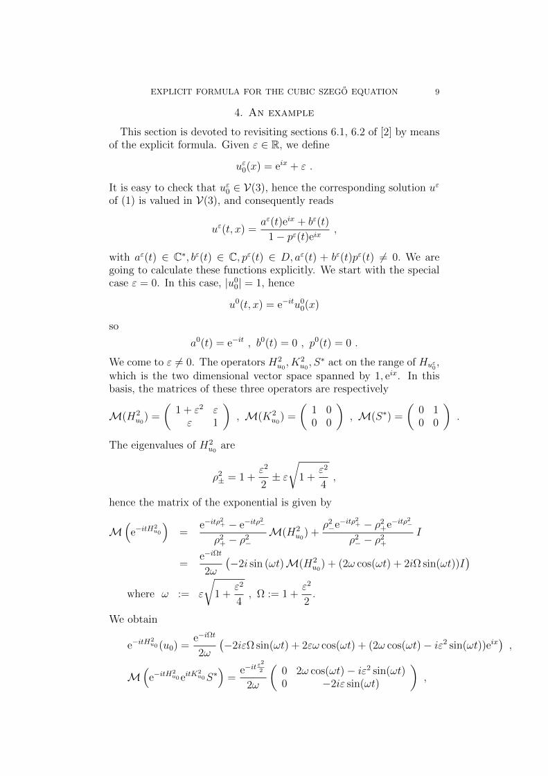
4. An example

This section is devoted to revisiting sections 6.1, 6.2 of [2] by meansof the explicit formula. Given ε ∈ R, we define

uε0(x) = eix + ε .

It is easy to check that uε0 ∈ V(3), hence the corresponding solution uε

of (1) is valued in V(3), and consequently reads

uε(t, x) =aε(t)eix + bε(t)

1− pε(t)eix,

with aε(t) ∈ C∗, bε(t) ∈ C, pε(t) ∈ D, aε(t) + bε(t)pε(t) 6= 0. We aregoing to calculate these functions explicitly. We start with the specialcase ε = 0. In this case, |u0

0| = 1, hence

u0(t, x) = e−itu00(x)

so

a0(t) = e−it , b0(t) = 0 , p0(t) = 0 .

We come to ε 6= 0. The operators H2u0, K2

u0, S∗ act on the range of Huε0

,which is the two dimensional vector space spanned by 1, eix. In thisbasis, the matrices of these three operators are respectively

M(H2u0

) =

(1 + ε2 εε 1

), M(K2

u0) =

(1 00 0

), M(S∗) =

(0 10 0

).

The eigenvalues of H2u0

are

ρ2± = 1 +

ε2

2± ε√

1 +ε2

4,

hence the matrix of the exponential is given by

M(

e−itH2u0

)=

e−itρ2+ − e−itρ

2−

ρ2+ − ρ2

−M(H2

u0) +

ρ2−e−itρ

2+ − ρ2

+e−itρ2−

ρ2− − ρ2

+

I

=e−iΩt

2ω

(−2i sin (ωt)M(H2

u0) + (2ω cos(ωt) + 2iΩ sin(ωt))I

)where ω := ε

√1 +

ε2

4, Ω := 1 +

ε2

2.

We obtain

e−itH2u0 (u0) =

e−iΩt

2ω

(−2iεΩ sin(ωt) + 2εω cos(ωt) + (2ω cos(ωt)− iε2 sin(ωt))eix

),

M(

e−itH2u0eitK

2u0S∗

)=

e−itε2

2

2ω

(0 2ω cos(ωt)− iε2 sin(ωt)0 −2iε sin(ωt)

),


Figure 4.1. The trajectory of pε for small ε.

and finally

aε(t) = e−it(1+ε2) , bε(t) = e−it(1+ε2/2)

(ε cos(ωt)− i 2 + ε2

√4 + ε2

sin(ωt)

)pε(t) = − 2i√

4 + ε2sin(ωt) e−itε

2/2 , ω :=ε

2

√4 + ε2 .

The important feature of such dynamics concerns the regime ε → 0.Though p0(t) ≡ 0, pε(t) may visit small neighborhoods of the unitcircle at large times. Specifically, at time tε = π/(2ω) ∼ π/(2ε), wehave |pε(t)| ∼ 1− ε2. A consequence is that the momentum density,

µn(tε) := n|uε(tε, n)|2 = n|aε(tε) + bε(tε)pε(tε)|2|pε(tε)|2(n−1)

= nε4

(4 + ε2)2

(1− ε2

4 + ε2

)n−1

,

which satisfies∞∑n=1

µn(tε) = Tr(K2uε(tε)) = Tr(K2

uε0) = 1 ,

becomes concentrated at high frequencies

n ' 1

ε2.

This induces the following instability of Hs norms

‖uε(tε)‖Hs ' 1

ε2s−1, s >

1

2,

a phenomenon of the same nature as the one displayed by Colliander,Keel, Staffilani, Takaoka and Tao in [1]. This proves in particular that


conservation laws do not control Hs regularity for s > 12. Notice that,

as already mentioned at the end of subsection 1.3 of the introduction,the family (uε0) approaches u0

0, which is a non generic element of V(3),since H2

u0admits 1 as a double eigenvalue.

This example naturally leads to the question of large time behavior ofthe Hs norm of individual solutions for s > 1

2. We are going to answer

this question in the special case of finite rank solutions by proving thequasi periodicity theorem in the next two sections.

5. Generalization to the Szego hierarchy

The Szego hierarchy was introduced in [2] and used in [3]. For theconvenience of the reader, and because our notation is slightly different,

we shall recall the main facts here. For y > 0 and u ∈ H12+, we set

Jy(u) = ((I + yH2u)−1(1)|1) .

Notice that the connection with the Szego equation is made by

E(u) =1

4(∂2yJ

y|y=0 − (∂yJ

y|y=0)2) .

For every s > 12, Jy is a smooth real valued function on Hs

+, and itsHamiltonian vector field is given by

XJy(u) = 2iywyHuwy , wy := (I + yH2

u)−1(1) ,

which is a Lipschitz vector field on bounded subsets of Hs+. This fact is

a consequence of the following lemma, where we collect basic estimates.We recall that the Wiener algebra W is the space of f ∈ L2

+ such that

‖f‖W :=∞∑k=0

|f(k)| <∞ .

Lemma 2. Let f, u, v ∈ L2+.

‖Huf‖W ≤ ‖u‖W‖f‖W ,

‖Huf‖Hs− 12≤ ‖u‖Hs‖f‖L2 , s ≥ 1

2,

‖Huf‖Hs ≤ ‖u‖Hs‖f‖W , s ≥ 0 ,

‖wy‖Hs ≤ (1 + y‖u‖2Hs) , s > 1 ,

‖fg‖Hs ≤ Cs(‖f‖W‖g‖Hs + ‖g‖W‖f‖Hs) ,

‖XJy(u)−XJy(v)‖Hs ≤ Cs(R, y)‖u− v‖Hs , s > 1 , ‖u‖Hs + ‖v‖Hs ≤ R .

Proof. The first three estimates are straightforward consequences ofthe formula

Huf(k) =∞∑`=0

u(k + `)f(`) .


The fourth estimate comes from these estimates and the fact that

wy = 1− yH2uw

y , ‖wy‖L2 ≤ 1 .

The fifth estimate is obtained by decomposing

f g(k) =∞∑`=0

f(k − `)g(`) =∑|k−`|≤`

f(k − `)g(`) +∑|k−`|>`

f(k − `)g(`) .

As for the last estimate, we set

wy[u] := (I + yH2u)−1(1) .

We write

‖wy[u]−wy[v]‖L2 = y‖(I+yH2u)−1(H2

v−H2u)(I+yH2

v )−1(1)‖L2 ≤ yR‖u−v‖Hs .

Then, by using again the first two inequalities,

wy[u]− wy[v] = y(H2v (wy[v])−H2

u(wy[u]))

leads to

‖wy[u]− wy[v]‖Hs ≤ C(R, y)‖u− v‖Hs .

Using moreover the fact that Hs is an algebra, this yields the desiredestimate.

By the Cauchy–Lipschitz theorem, the evolution equation

(14) u = XJy(u)

admits local in time solutions for every initial data in Hs+ for s > 1,

and the lifetime is bounded from below if the data are bounded in Hs+.

We shall see that this evolution equation admits a Lax pair structuresimilar to the one in section 2.

Theorem 4. For every u ∈ Hs+, we have

HiXJy (u) = HuFyu + F y

uHu ,

KiXJy (u) = KuGyu +Gy

uKu ,

Gyu(h) := −ywy Π(wy h) + y2Huw

y Π(Huwy h) ,

F yu (h) := Gy

u(h)− y2(h|Huwy)Huw

y .

If u ∈ C∞(I, Hs+) is a solution of equation (14) on a time interval I,

then

dHu

dt= [By

u, Hu] ,dKu

dt= [Cy

u, Ku] ,

Byu = −iF y

u , Cyu = −iGy

u .

Proof.

Lemma 3. We have the following identity,

HaHu(a)(h) = Hu(a)Ha(h) +Hu(aΠ(ah)− (h|a)a) .


Proof.

HaHu(a)(h) = Π(aHu(a)h) = Hu(a)Ha(h) + Π(Hu(a)(I − Π)(ah)) .

On the other hand,

(1− Π)(ah) = Π(ah)− (a|h) .

The lemma follows by plugging the latter formula into the former one.

Let us complete the proof. Using the identity

wy = 1− yH2uw

y,

and Lemma 3 with a = Hu(wy), we get

Hwy Hu(wy)(h) = HHu(wy)(h)− yHHu(wy)H2u(wy)(h)

= HHu(wy)(h)− yH2u(wy)HHu(wy)(h)− yHu

(Hu(w

y)Π(Hu(wy)h)− (h|Hu(wy))Hu(w

y))

= wyHHu(wy)(h)− yHu

(Hu(w


y))

= wy Π(wyHuh)− yHu

(Hu(w


y)).

We therefore have obtained

Hwy Hu(wy) = LyuHu +HuRyu

where Lyu and Ryu are the following self adjoint operators,

Lyu(h) = wy Π(wy h) , Ryu(h) = −y

(Hu(w


y)).

Consequently, since Hwy Hu(wy) is self adjoint,

Hwy Hu(wy) =1

2(Lyu +Ry

u)Hu +Hu1

2(Lyu +Ry

u) .

Multiplying by −2y, we obtain the desired formula, since

F yu = −y(Lyu +Ry

u) .

We now come to the second identity. From the first one, we get

(15) KiXJy (u) = HiXJy (u)S = HuFyuS + F y

uKu .

For every h, v ∈ L2+, we use

Π(vSh) = SΠ(vh) + (Sh|v)

and infer

F yuSh = −ywy Π(wy Sh) + y2Huw

y Π(Huwy Sh)− y2(Sh|Huwy)Huw

y

= SGyuh− y(Sh|wy)wy = SGy

uh+ y2(Sh|H2uw

y)wy

= SGyuh+ y2(Hu(w

y)|Ku(h))wy ,

where we have used wy = 1− yH2uw

y again. Plugging this identity into(15), we obtain the claim.


The last formulae are straightforward consequences of the antilinearityof Hu and Ku.

Using Theorem 4 in a similar way to section 2, we derive

Corollary 2. Under the conditions of Theorem 4, assuming moreover0 ∈ I, define Uy = Uy(t), V y = V y(t) the solutions of the followinglinear ODEs on L(L2

+),

dUy

dt= By

u Uy ,

dV y

dt= Cy

u Vy , Uy(0) = V y(0) = I .

Then Uy(t), V y(t) are unitary operators and

Hu(t) = Uy(t)Hu(0)Uy(t)∗ , Ku(t) = V y(t)Ku(0)V

y(t)∗ .

At this stage, we are going to generalize slightly the setting, for theneeds of the next section. Let y1, . . . , yn be positive numbers, anda1, . . . , an be real numbers. We consider the functional

J(u) =n∑k=1

akJyk(u) = (f(H2

u)1|1) , f(s) :=n∑k=1

ak1 + yks

,

and the evolution equation

(16) u = XJ(u) .

By linearity from Theorem 4, it is clear that the solution of (16) satisfies

(17)dHu

dt= [Bu, Hu] ,

dKu

dt= [Cu, Ku] ,

with

(18) Bu =n∑k=1

akByku , Cu =

n∑k=1

akCyku .

Corollary 3. Let u be a solution of equation (16) on some time in-

terval I containing 0, define U = U(t), V = V (t) the solutions of thefollowing linear ODEs on L(L2

+),

dU

dt= Bu U ,

dV

dt= Cu V , U(0) = V (0) = I .

Then U(t), V (t) are unitary operators and

Hu(t) = U(t)Hu(0)U(t)∗ , Ku(t) = V (t)Ku(0)V (t)∗ .

As a consequence of this corollary, if we start from an initial datumu(0) such that Hu(0) is a trace class operator, then Hu(t) is trace classfor every t, with the same trace norm. By Peller’s theorem [11], Chap.6, Theorem 1.1, the trace norm of Hu is equivalent to the norm of uin the Besov space B1

1,1, which is contained into W and contains Hs+

for every s > 1. Consequently, if u(0) ∈ Hs+ for some s > 1, then u(t)

stays bounded in W . We claim that, if u(0) is in V(d), the evolution


can be continued for all time. Moreover, since the ranks of Hu(t) andKu(t) are conserved in view of Corollary 3, this evolution takes place inV(d) if u(0) ∈ V(d).

Corollary 4. The equation (16) defines a smooth flow on Hs+ for every

s > 1 and on V(d) for every d.

In view of the Gronwall lemma, the statement is an easy consequenceof the following estimate.

Lemma 4. Let R, y ≥ 0, s > 1 be given. There exists C(d,R, y, s) > 0such that, for every u ∈ V(d) with ‖u‖W ≤ R,

‖XJy(u)‖Hs ≤ C(d,R, y, s)(1 + ‖u‖Hs) .

Proof. By using Lemma 2, we are reduced to prove

‖wy‖W ≤ B(d,R, y) .

We set N =[d+1

2

]. The above estimate is an easy consequence of

(I +H2u)−1 =

N∑k=0

akH2ku ,

with |ak| ≤ 1 for k = 0, . . . , N . In fact, the Cayley–Hamilton theoremyields

(H2u)N+1 =

N∑k=1

(−1)k−1Sk(H2u)N−k+1 , Sk :=

∑`1<···<`k

ρ2`1. . . ρ2

`k,

and one can easily check that

ak = (−1)k

1 +N−k∑j=1

Sj

1 +N∑j=1

Sj

, k = 0, . . . , N .

where ρ21 ≥ · · · ≥ ρ2

N are the positive eigenvalues of H2u, listed with

their multiplicities.

Remark 1. For general data u(0) ∈ Hs+, one can prove similarly that

the solution can be continued for all time if y‖u(0)‖Hs is small enough,or just if yTr|Hu(0)| is small enough.

Our next step is to derive an explicit formula for the solution of(16) along the same lines as in section 3. The starting points are theformulae

Byu(1) = iyJy(u)wy

Cyu −By

u = −iy2(·|Huwy)Huw

y

= iyJy(u)((I + yH2u)−1 − (I + yK2

u)−1) ,


where we have used the identity K2u = H2

u − (·|u)u . This leads to

Bu(1) = ig(H2u)(1) , g(s) :=

n∑k=1

akykJyk(u)

1 + yks,

Cu − Bu = i(g(H2u)− g(K2

u)) .

Arguing exactly as in section 3, we obtain the following formula.

Theorem 5. The solution u of equation (16) with initial data u(0) =u0 ∈ Hs

+, s > 1, is given by

(19) u(t, z) = ((I − ze2itg(H2u0

)e−2itg(K2u0

)S∗)−1e2itg(H2u0

)u0 | 1) , z ∈ D ,

where

g(s) :=n∑k=1

akykJyk(u)

1 + yks.

6. Proof of the quasiperiodicity theorem

In this section, we prove Theorem 2. Let u0 ∈ V(d) be given. Firstlywe show that t 7→ u(t) is a quasi periodic function valued into V(d).Denote by Σ the union of the spectra of H2

u0and K2

u0. We claim that

it is enough to prove that, for any function ω : Σ→ T, the formula

Φ(ω)(z) = ((I − ze−iω(H2u0

)eiω(K2u0

)S∗)−1e−iω(H2u0

)u0 | 1) , z ∈ D ,

defines an element Φ(ω) ∈ V(d). Indeed, if this is established, Theorem1 exactly claims that u(t) = Φ(tω), where, for every s ∈ Σ, ω(s) =s mod 2π . Moreover, it is clear from the above formula that Φ(ω) is arational function with coefficients smoothly dependent on ω ∈ TΣ, sothat Φ is smooth as a map from TΣ to V(d).

Let ω ∈ TΣ. For each s ∈ Σ, we represent ω(s) by some elementof [0, 2π), still denoted by ω(s). Fix n = |Σ| and let y1, . . . , yn be npositive numbers pairwise distinct. Then the matrix(

1

1 + yks

)k=1,...,n,s∈Σ

is invertible, hence the linear system

ω(s) = −2n∑k=1

akykJyk(u0)

1 + yks, s ∈ Σ

has a unique solution a1, . . . , an. Using Theorem 5, Φ(ω) is the valueat time t = 1 of the solution u of equation (16) with parametersa1, . . . , an, y1, . . . , yn. By Corollary 4, it belongs to V(d). This provesquasi periodicity.

Since Φ is a continuous mapping, Φ(TΣ) is a compact subset of V(d).On the other hand, for every s, the Hs norm is continuous on V(d). It is


therefore bounded on this compact subset, which contains the integralcurve issued from u0. This completes the proof of Theorem 2.

Remark 2. It is tempting to adapt the above proof of quasi periodicityto non finite rank solutions. However, even assuming that one candefine a flow on Hs

+ for all y with convenient estimates for large y,this strategy meets a serious difficulty. Indeed, on the one hand, theconstruction of a Hamiltonian flow on Hs

+ for

J(u) = (f(H2u)1|1)

requires a minimal regularity for f , say C1, which, if f is representedas

f(s) =

∞∫0

a(y)

1 + ysdµ(y)

for some positive measure µ and some function a on R+, imposes adecay condition as

∞∫0

y|a(y)| dµ(y) .

On the other hand, Σ is made of a sequence of positive numbers con-verging to 0 and of its limit, and the interpolation problem

ω(s) = −2

∞∫0

ya(y)Jy(u0)

1 + ysdµ(y)

would have a solution only if ω : Σ → T is continuous on Σ. Un-fortunately, the space C(Σ,T) is not compact, neither for the simpleconvergence, nor for the uniform convergence. Therefore the questionof large time dynamics of non finite rank solutions of the cubic Szegoequation remains widely open.

References

[1] Colliander J., Keel M., Staffilani G., Takaoka H., Tao, T., Transfer ofenergy to high frequencies in the cubic defocusing nonlinear Schrodingerequation, Inventiones Math.181 (2010), 39–113.

[2] Gerard, P., Grellier, S., The cubic Szego equation , Ann. Scient. Ec. Norm.Sup. 43 (2010), 761-810.

[3] Gerard, P., Grellier, S., Invariant Tori for the cubic Szego equation, In-vent. math. 187 (2012), 707–754.

[4] Gerard, P., Grellier, S., Effective integrable dynamics for a certain non-linear wave equation, Analysis and PDEs, 5 (2012), 1139–1155.

[5] Kappeler, T., Poschel, J. : KdV & KAM, A Series of Modern Surveys inMathematics, vol. 45, Springer-Verlag, 2003.

[6] Kronecker, L. : Zur Theorie der Elimination einer Variabeln auszwei algebraischen Gleichungen Monatsber. Konigl. Preuss. Akad. Wiss.(Berlin), 535-600 (1881). Reprinted in Leopold Kronecker’s Werke, vol. 2,113–192, Chelsea, 1968.


[7] Lax, P. : Integrals of Nonlinear equations of Evolution and SolitaryWaves, Comm. Pure and Applied Math. 21, 467-490 (1968).

[8] Lax, P. : Periodic solutions of the the KdV equation. Comm. Pure Appl.Math. 28 , 141–188 (1975).

[9] Nikolskii, N. K. : Operators, functions, and systems: an easy reading.Vol. 1. Hardy, Hankel, and Toeplitz. Translated from the French by An-dreas Hartmann. Mathematical Surveys and Monographs, 92. AmericanMathematical Society, Providence, RI, 2002.

[10] Novikov, S. P. : The periodic problem for the Korteweg-de Vries equation.Funkt. Anal. i Prilozhen. 8 (1974), 54-66.

[11] Peller, V. V.: Hankel operators and their applications. Springer Mono-graphs in Mathematics. Springer-Verlag, New York, 2003.

[12] Zakharov, V. E., Shabat, A. B.: Exact theory of two-dimensional self-focusing and one-dimensional self-modulation of waves in nonlinear me-dia. Soviet Physics JETP 34 (1972), no. 1, 62–69.

Universite Paris-Sud XI, Laboratoire de Mathematiques d’Orsay,CNRS, UMR 8628, et Institut Universitaire de France

E-mail address: [email protected]

Federation Denis Poisson, MAPMO-UMR 6628, Departement de Mathematiques,Universite d’Orleans, 45067 Orleans Cedex 2, France

E-mail address: [email protected]

AN EXPLICIT FORMULA FOR THE CUBIC SZEGO … EXPLICIT FORMULA FOR THE CUBIC SZEGO EQUATION} PATRICK...

Documents

Transcript of AN EXPLICIT FORMULA FOR THE CUBIC SZEGO … EXPLICIT FORMULA FOR THE CUBIC SZEGO EQUATION} PATRICK...