An experimental study of ber suspensions between counter ...278629/FULLTEXT01.pdf · An...
87
An experimental study of fiber suspensions between counter-rotating discs by Charlotte Ahlberg November 2009 Technical Reports from Royal Institute of Technology KTH Mechanics SE-100 44 Stockholm, Sweden
Transcript of An experimental study of ber suspensions between counter ...278629/FULLTEXT01.pdf · An...

An experimental study of fiber suspensionsbetween counter-rotating discs
by
Charlotte Ahlberg
November 2009Technical Reports from
Royal Institute of TechnologyKTH Mechanics
SE-100 44 Stockholm, Sweden

Akademisk avhandling som med tillstand av Kungliga Tekniska Hogskolan iStockholm framlagges till offentlig granskning for avlaggande av teknologielicentiatexamen fredagen den 4 december 2009 kl 10.15 i Sundbladsalen,Drottning Kristinas vag 61, Innventia AB, Stockholm.
c©Charlotte Ahlberg 2009Universitetsservice US–AB, Stockholm 2009

An experimental study of fiber suspensions between counter-rotating discs
Charlotte Ahlberg 2009,KTH MechanicsSE-100 44 Stockholm, Sweden
Abstract
The behavior of fibers suspended in a flow between two counter-rotating discshas been studied experimentally. This is inspired by the refining process in thepapermaking process where cellulose fibers are ground between discs in orderto change performance in the papermaking process and/or qualities of the finalpaper product.
To study the fiber behavior in a counter-rotating flow, an experimental set-up with two glass discs was built. A CCD-camera was used to capture imagesof the fibers in the flow. Image analysis based on the concept of steerable filtersextracted the position and orientation of the fibers in the plane of the discs.Experiments were performed for gaps of 0.1 − 0.9 fiber lengths, and for equalabsolute values of the angular velocities for the upper and lower disc. Theaspect ratios of the fibers were 7, 14 and 28.
Depending on the angular velocity of the discs and the gap between them,the fibers were found to organize themselves in fiber trains. A fiber train is aset of fibers positioned one after another in the tangential direction with a closeto constant fiber-to-fiber distance. In the fiber trains, each individual fiber isaligned in the radial direction (i.e. normal to the main direction of the train).
The experiments show that the number of fibers in a train increases as thegap between the discs decreases. Also, the distance between the fibers in atrain decreases as the length of the train increases, and the results for shorttrains are in accordance with previous numerical results in two dimensions.Furthermore, the results of different aspect ratios imply that there are three-dimensional fiber end-effects that are important for the forming of fiber trains.
Descriptors: Fiber suspension flow, rotating discs, shear flow, self-organizationof fibers.

Enjoy!
iv

Preface
Parts of this work has been presented at
• APS (American Physics Society) Division of Fluid Dynamics annualconference November 25–27, 2008 in San Antonio, Texas, USA.
• SIAMUF (Swedish Industrial Association for Multiphase Fluids) con-ference May 13–14, 2009 in Alvkarleby, Sweden.
• SNM (Swedish National Committee for Mechanics) Svenska Mekanik-dagarna June 15–17, 2009 in Sodertalje, Sweden.
• ASME (American Society of Mechanical Engineering) Fluid EngineeringDivision Summer Meeting August 3–6, 20091 in Vail, Colorado, USA.
The supervisors have been L. D. Soderberg2 and F. Lundell3.
November 2009, StockholmCharlotte Ahlberg
1Written contribution to the conference proceedings: ”Self-organization of fibers in flow
between two counter-rotating discs”, C. Ahlberg, F. Lundell and L. D. Soderberg.2at Innventia AB and KTH Mechanics.3at KTH Mechanics.
v

vi

Contents
Abstract iii
Preface v
Chapter 1. Introduction 11.1. Short description of the papermaking process 11.2. Aim and scope of this thesis 5
Chapter 2. Background and previous work 92.1. Non-dimensional numbers 92.2. Similarity solution for flow between rotating discs 102.3. Characteristics of flow between rotating discs 142.4. Settling velocity 152.5. Fiber suspensions 162.6. Orientation of fibers in shear flow 172.7. Cylinders in shear flow 202.8. Pattern formations of particles in shear flow 22
Chapter 3. Experimental set-up, methods and data evaluation 253.1. Experimental set-up 253.2. Evaluation techniques 293.3. Experimental procedures and parameters 313.4. Characteristics of the flow 343.5. A note on statistical reliability of the data 35
Chapter 4. Results and discussion 394.1. Flow conditions 394.2. Orientation and position of fibers 404.3. Behavior and occurrence of fiber trains 45
vii
4.4. Distance between fibers in trains 514.5. Angle deviation of fibers in trains 554.6. Effect of fiber length 56
Chapter 5. Conclusions and outlook 59
Acknowledgements 61
References 63
Appendix A. Measurement data 67
Appendix B. Position-orientations pictures 71
viii
CHAPTER 1
Introduction
This licentiate thesis deals with the orientation and behavior of fibers suspendedin the shear flow between two rotating, closely spaced and parallel flat discs.Experiments have been performed and show a complicated interaction betweenthe flow, the solid walls and the solid fibers, where the fibers are seen to formpatterns. The results have been analyzed and compared to other publishedstudies.
This research has been inspired by the papermaking industry, where therefining stage in the papermaking process includes fiber suspension flow innarrow conduits. The work can also be related to other areas where pattern-forming of rod-like particles are in focus. For example, lubrication of bearingsis one area where pattern formation of particles can be of importance. There,minimization of energy loss due to friction is the goal and present researchconcerns liquid crystals forming patterns that improve lubrication and minimizethe friction, see Abrahamson (2008).
1.1. Short description of the papermaking process
In order to be able to view this thesis as part of a greater whole, a briefdescription of the pulp and papermaking process follows. A simplified andschematic picture of the papermaking process is shown in Fig. 1.1.
First, the pulp is produced and the process starts with removing the outerinsulating and protective layer on the tree trunk, i.e. the bark, which is donein a debarker. The wood is then chopped into chips and treated in order toliberate the individual cellulose fibers. For mechanical pulp this is done bygrinding and heat treatment, and for chemical pulp, chemicals are used insteadof grinding. There can also be a combination of these treatments. At this pointin the manufacturing process, the pulp, i.e. the suspension, consists of cellulosefibers and water that can be delivered to the papermaking plant.
In the papermaking process, Fig. 1.1, the delivered pulp is worked up to apulp suspension. Chemicals are added in order to modify the fibers to improvedesired qualities, e.g. the dewatering ability within the paper process or tensileindex and light-scattering abilities of the product, see e.g. Norman & Fellers(1998). The suspension is then ground in a refiner to nap the surfaces of the
1

2 1. INTRODUCTION
Figure 1.1. Overview of the pulp and paper making process.
(a) (b)
Figure 1.2. Chemical pulp fibers (a) before and (b) after therefining process.
fibers. There are two types of refiners, high consistency (HC) and low consis-tency (LC) refiners, where the pulp concentration in a HC refiner is typically25−35% and 2−6% in a LC refiner. When the refining and fractionation stepshave produced a satisfactory suspension, it is jetted out, through a headboxand out onto a wire, as a thin suspension sheet. The dewatering on the wiremakes the fibers form a network on it, giving a fiber mat that starts to looklike paper. Mechanical dewatering squeezes out the remaining water throughpressing and after that, water still trapped in the fibers is evaporated in thedrying section. After the dewatering stages, the surface of the paper can beimproved in mainly two ways, either by calendering, where the surface is im-proved mechanically by being pressed between several cylinders, or by coating,where a coat is added onto the paper surface. The final stage is the winding ofthe finished paper onto a reel at the reel-up.
1.1. SHORT DESCRIPTION OF THE PAPERMAKING PROCESS 3
(a) (b)
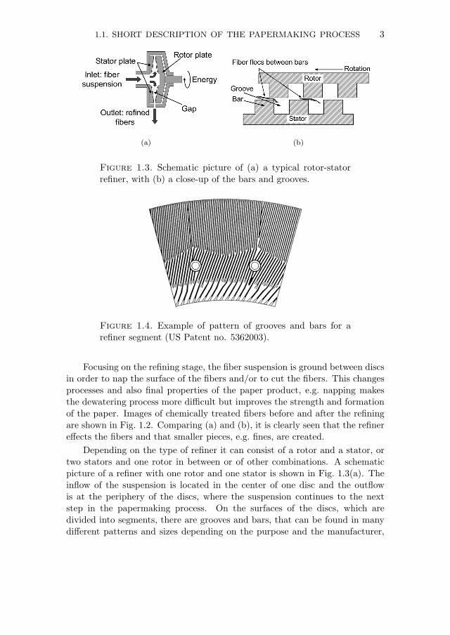
Figure 1.3. Schematic picture of (a) a typical rotor-statorrefiner, with (b) a close-up of the bars and grooves.
Figure 1.4. Example of pattern of grooves and bars for arefiner segment (US Patent no. 5362003).
Focusing on the refining stage, the fiber suspension is ground between discsin order to nap the surface of the fibers and/or to cut the fibers. This changesprocesses and also final properties of the paper product, e.g. napping makesthe dewatering process more difficult but improves the strength and formationof the paper. Images of chemically treated fibers before and after the refiningare shown in Fig. 1.2. Comparing (a) and (b), it is clearly seen that the refinereffects the fibers and that smaller pieces, e.g. fines, are created.
Depending on the type of refiner it can consist of a rotor and a stator, ortwo stators and one rotor in between or of other combinations. A schematicpicture of a refiner with one rotor and one stator is shown in Fig. 1.3(a). Theinflow of the suspension is located in the center of one disc and the outflowis at the periphery of the discs, where the suspension continues to the nextstep in the papermaking process. On the surfaces of the discs, which aredivided into segments, there are grooves and bars, that can be found in manydifferent patterns and sizes depending on the purpose and the manufacturer,
4 1. INTRODUCTION
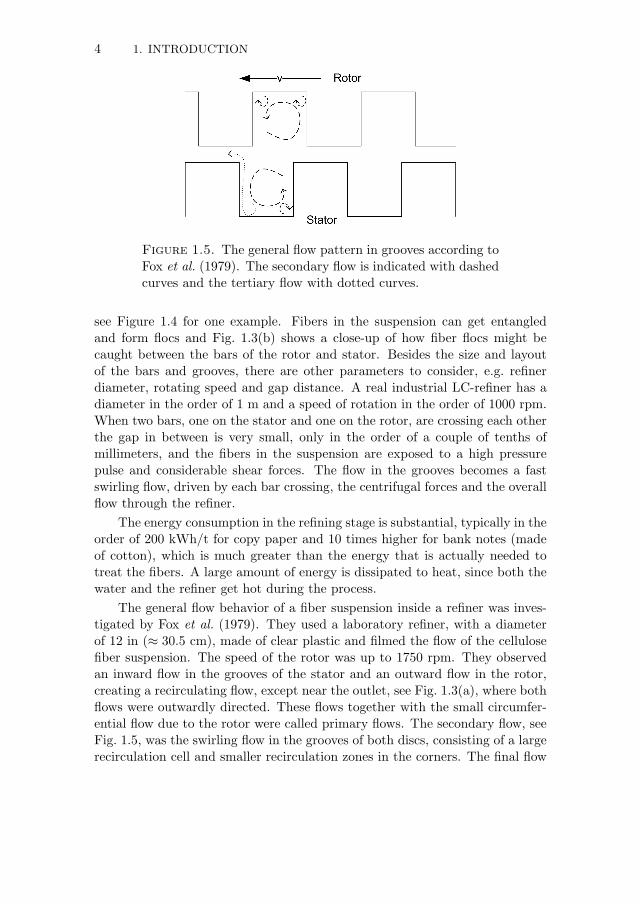
Figure 1.5. The general flow pattern in grooves according toFox et al. (1979). The secondary flow is indicated with dashedcurves and the tertiary flow with dotted curves.
see Figure 1.4 for one example. Fibers in the suspension can get entangledand form flocs and Fig. 1.3(b) shows a close-up of how fiber flocs might becaught between the bars of the rotor and stator. Besides the size and layoutof the bars and grooves, there are other parameters to consider, e.g. refinerdiameter, rotating speed and gap distance. A real industrial LC-refiner has adiameter in the order of 1 m and a speed of rotation in the order of 1000 rpm.When two bars, one on the stator and one on the rotor, are crossing each otherthe gap in between is very small, only in the order of a couple of tenths ofmillimeters, and the fibers in the suspension are exposed to a high pressurepulse and considerable shear forces. The flow in the grooves becomes a fastswirling flow, driven by each bar crossing, the centrifugal forces and the overallflow through the refiner.
The energy consumption in the refining stage is substantial, typically in theorder of 200 kWh/t for copy paper and 10 times higher for bank notes (madeof cotton), which is much greater than the energy that is actually needed totreat the fibers. A large amount of energy is dissipated to heat, since both thewater and the refiner get hot during the process.
The general flow behavior of a fiber suspension inside a refiner was inves-tigated by Fox et al. (1979). They used a laboratory refiner, with a diameterof 12 in (≈ 30.5 cm), made of clear plastic and filmed the flow of the cellulosefiber suspension. The speed of the rotor was up to 1750 rpm. They observedan inward flow in the grooves of the stator and an outward flow in the rotor,creating a recirculating flow, except near the outlet, see Fig. 1.3(a), where bothflows were outwardly directed. These flows together with the small circumfer-ential flow due to the rotor were called primary flows. The secondary flow, seeFig. 1.5, was the swirling flow in the grooves of both discs, consisting of a largerecirculation cell and smaller recirculation zones in the corners. The final flow

1.2. AIM AND SCOPE OF THIS THESIS 5
or tertiary flow, see Fig. 1.5, was directed from the corner of a groove (wherethe smaller recirculation zones are) in the stator towards and past the cornerof the nearest bar. In addition to this qualitative description of the flow of thesuspension, the behavior of the fibers was also qualitatively described by Foxet al. (1979). They observed that at a specific radius, the fibers were stapledto the bars of either the rotor or the stator, and concluded that the tertiaryflow held the fibers to the bars and it was mainly these stapled fibers that wererefined.
Later, Koskenhely et al. (2005) studied the effects of different ways ofrefining different fractions of bleached softwood kraft pulp; a 56/44% mixtureof pine/spruce fibers. Fiber length, fiber cross-sections, fines content, amount ofwater in the cell wall of the cellulose fiber and cell wall thickness were measuredfor the different pulp fractions. Several connections between paper propertiesand selective refining could be seen, e.g. that the fiber shortening was mostsevere for higher intensities. However, it was not clear whether the cuttingwas due to high tension or to the bar edges, or if it was a fatigue process or asingle-event phenomenon.
Though there are many more studies with cellulose fibers and refiners, theydeal mainly with the material (pulp) input contra the material output of therefiner and not the treatment inside it. At this point in the review it canbe concluded that it is not known what physical events that treat the fibersnor the details of how the fiber suspension behaves inside a refiner. It is acomplex environment with many parameters. Due to this, the refining processin industry can, at the present time, be considered to be an art, based onknowledge and experience. The refiner at a plant is adjusted based on theinformation of the input pulp and by knowing the behavior of the refiner atthat particular plant. Then, the output of the refiner becomes the desired,perhaps after some iterative adjustments.
1.2. Aim and scope of this thesis
The aim of this thesis is to investigate what the flow looks like and how thefibers behave in a basic geometry, similar to what can be found inside a refiner,but at lower velocities. The vision is of course to completely understand the flowinside the real refiner and more important the treatment of the fibers. Then,it would be possible not only to predict the result of the refining without trialand error, but also to improve the process and to save energy. One can alsohypothesize that improved understanding of the refining process will revealthe physical reasons behind the effects. With such knowledge, the desiredphysical fiber treatments might be possible to achieve more efficiently in somecompletely different device.
6 1. INTRODUCTION
As described in the previous section, a real refiner with all its parametersis a very complicated environment. In order to increase the knowledge andunderstanding, it is necessary to start with a basic case with few parametersthat can be controlled. Only then is it possible to introduce more parametersone after another and gradually build up a more complicated environment andto understand it. However, there seem to be a lack of fundamental research offibers in shear and rotating flows in the literature.
In order to approach our vision we proceed according to the followingstrategy regarding the experimental set-up and parameter range:
1. Basic geometry, low Reynolds numbers1
2. More complex geometry, low Reynolds numbers3. More complex geometry, increasing Reynolds numbers
This thesis is the first step of the strategy, where the basic geometry of theexperimental set-up consists of two coaxial flat discs, exactly counter-rotating2
and separated by a small gap distance. The gap between the two flat discsare often simply called ‘the gap’. Single phase flow in this geometry has beenstudied extensively. Thus, the flow in the present study is well established andwill be described in the review in section 2.2. To understand the behavior offibers in a suspension, parts dealing with a falling fiber in quiescent fluid, char-acteristics of fiber suspensions, cylinders in shear flow and pattern formationsare included in this work.
Furthermore and concerning the fibers in the suspension, real cellulosefibers would have shown too large deviations in length, thickness and stiffness,which in turn would have introduced too many unknown parameters. There-fore, artificial fibers with a well-defined length and thickness have been used inthis work.
During the initial observations of the fiber behavior in this thin and rotatingenvironment, we discovered that the fibers tend to form patterns, and the latterpart of this work came to focus on the occurrence and structure of these fiberpatterns.
This thesis continues with a review of relevant fluid mechanical studiesof flow between rotating discs and particles in shear flow in chapter 2. Theexperimental apparatus and methods, including data evaluation, are describedin chapter 3. In chapter 4 the results are presented and discussed before theconclusions are stated in chapter 5 together with an outlook. Two appendices
1Using Reynolds number is one way to characterize the flow and is the ratio between the
inertial and viscous terms in the Navier-Stokes equations for an incompressible fluid.2with exactly counter-rotating is meant that the absolute values of the angular velocities of
the upper and lower disc are the same.

1.2. AIM AND SCOPE OF THIS THESIS 7
are included: the first is a complete overview of all parameter combinationsstudied and the second is the complete data on fiber position and orientation.

8

CHAPTER 2
Background and previous work
This review chapter starts with single-phase flow between counter-rotating discsand continues with fiber suspensions and orientations of slender bodies in con-fined shear flow. Finally, work concerning pattern formation of particles inshear flow are reviewed.
2.1. Non-dimensional numbers
In order to study the problem of a fiber suspension in between counter-rotatingdiscs, schematically illustrated in Fig. 2.1, we define the following set of non-dimensional numbers:
• ReH = 2hR∆Ω/ν as a gap Reynolds number, where 2h is the verticalgap distance between the discs, R is the radial coordinate, ∆Ω = |Ωup|+|Ωlow| is the difference between the angular velocity of the upper disc,Ωup(> 0), and the angular velocity of the lower disc, Ωlow(< 0). ν isthe kinematic viscosity of the fluid.
• R = h2Ω/ν as a second gap Reynolds number, where Ω = ∆Ω/2.• Reφ = ∆ΩR2/ν as a rotational Reynolds number.• Rep = γ a2/ν as a particle Reynolds number, where a is the radius of a
fiber and γ is the shear rate, γ = R Ω/h.• G = 2h/R2 as a gap ratio, where R2 is the radius of the upper disc.• λ = 2h/L as the ratio between the gap and the length of a fiber, L.• α = L/d as the aspect ratio for a fiber, where d = 2a.• ξ = ρp/ρf as the ratio between the density of the particles, ρp and the
density of the fluid, ρf .
Having a two disc problem with a gap in between, we also define
s =ΩupΩlow
(2.1)
Hence, s = −1 in the case of exactly counter-rotating discs, i.e. when |Ωup| =|Ωlow|, and s = 1 is the case of equally rotating discs, i.e. the case whereΩup = Ωlow and we would obtain a solid body rotation as the steady statesolution.
9

10 2. BACKGROUND AND PREVIOUS WORK
Figure 2.1. Schematic drawing of the problem.
2.2. Similarity solution for flow between rotating discs
The flow between two counter-rotating discs is assumed steady and rotation-ally symmetric and the dimensional cylindrical coordinates are (R,φ, Z). Thecenters of the discs are at Z = h and Z = −h, respectively. If we denote thedimensional velocity vector u = uer + veφ +wez, the Navier-Stokes equationsare:
u∂u
∂R+ w
∂u
∂Z− v2
R= −1
ρ
∂p
∂R+ ν
(∇2u− u
R2
)(2.2)
u
R
∂
∂R(Rv) + w
∂v
∂Z= ν
(∇2v − v
R2
)(2.3)
u∂w
∂R+ w
∂w
∂Z= −1
ρ
∂p
∂Z+ ν∇2w (2.4)
The continuity equation is:
∂
∂R(Ru) +
∂
∂Z(Rw) = 0 (2.5)
and the Laplace operator is:
∇2 =1R
∂
∂R
(R∂
∂R
)+
∂2
∂Z2(2.6)
The pressure can be eliminated by cross-differentiation of eqs. (2.2) and(2.4), giving:
∂
∂Z
u∂u
∂R+ w
∂u
∂Z− v2
R− ν
(∇2u− u
R2
)=
=∂
∂R
(u∂w
∂R+ w
∂w
∂Z− ν∇2w
)(2.7)

2.2. SIMILARITY SOLUTION FOR FLOW BETWEEN ROTATING DISCS 11
The continuity equation will be satisfied if we take:
u =1R
∂Ψ∂Z
(2.8)
w = − 1R
∂Ψ∂R
(2.9)
Putting eqs. (2.8) and (2.9) into eqs. (2.7) and (2.3), gives us two equationswith two unknowns; v and Ψ.
Assuming that both discs are of radius R2 and that the gap ratio G 1, wecan assume that the edge effects can be neglected, i.e. assuming that the discsare infinitely large in the sense that G ≈ 0. The radial and vertical coordinatesare non-dimensionalized with the length h, i.e. r = R/h and z = Z/h wherer and z are non-dimensional coordinates. The velocities are scaled with hΩ,i.e. u = u/hΩ, v = v/hΩ and w = w/hΩ. One can now assume that thenon-dimensional velocity field u = uer + veφ + wez) is of the following form,using the similarity ansatz of von Karman (1921), see e.g. Greenspan (1990) orHoffman (1974):
u = −12Rr
dHdz
(z) (2.10)
v = rG(z) (2.11)
w = RH(z) (2.12)
where G(z) and H(z) are non-dimensional functions and eqs. (2.10)–(2.12) au-tomatically satisfies the non-dimensional continuity equation, which is eq. (2.5),that after substitution to the non-dimensional variables becomes the same butwith the non-dimensional coordinates and velocities.
Substituting eqs. (2.10)–(2.12) into the Navier-Stokes equations gives thefollowing expressions for G and H:
d4Hdz4
= 4G dGdz
+ R2Hd3Hdz3
(2.13)
d2Gdz2
= R2
(HdGdz− G dH
dz
)(2.14)
The no-slip condition at the discs (z = ±1) in terms of G and H becomes, forexactly counter-rotating discs:
G(±1) = ±1, H(±1) = 0,dHdz
(±1) = 0 (2.15)
The algorithm for solving this system of equations was outlined by Hoff-man (1974), but has here been solved using spectral collocation method and
12 2. BACKGROUND AND PREVIOUS WORK
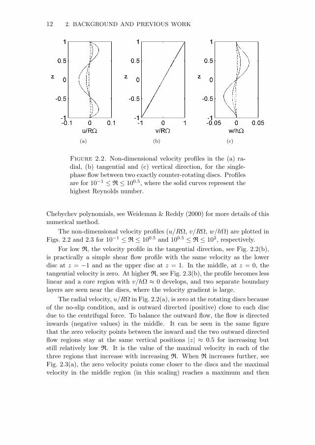
(a) (b) (c)
Figure 2.2. Non-dimensional velocity profiles in the (a) ra-dial, (b) tangential and (c) vertical direction, for the single-phase flow between two exactly counter-rotating discs. Profilesare for 10−1 ≤ R ≤ 100.5, where the solid curves represent thehighest Reynolds number.
Chebychev polynomials, see Weideman & Reddy (2000) for more details of thisnumerical method.
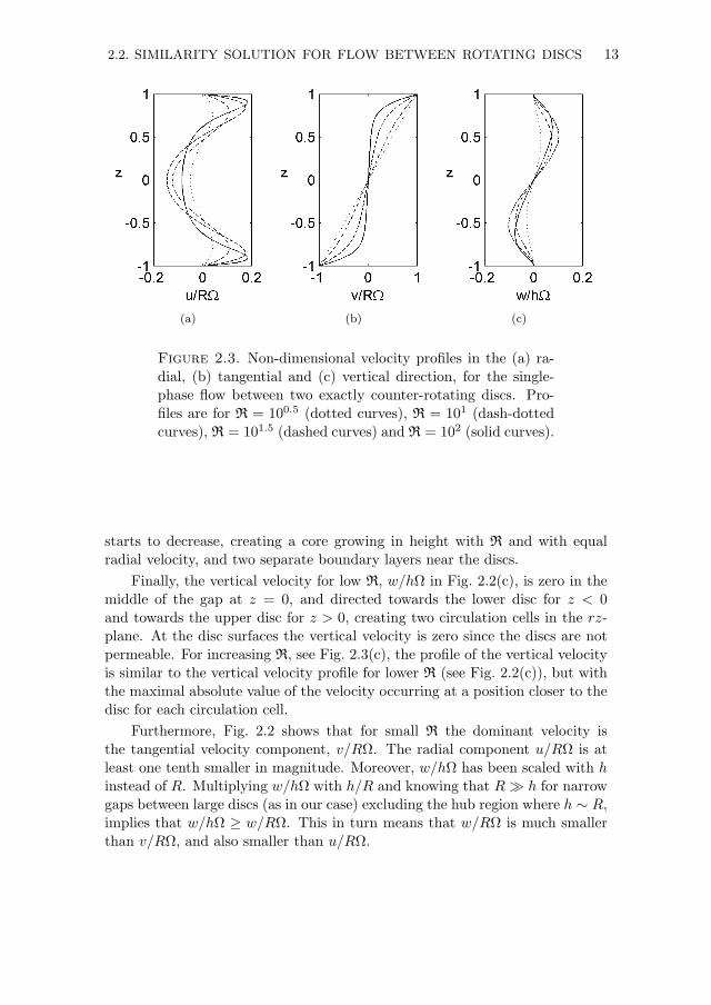
The non-dimensional velocity profiles (u/RΩ, v/RΩ, w/hΩ) are plotted inFigs. 2.2 and 2.3 for 10−1 ≤ R ≤ 100.5 and 100.5 ≤ R ≤ 102, respectively.
For low R, the velocity profile in the tangential direction, see Fig. 2.2(b),is practically a simple shear flow profile with the same velocity as the lowerdisc at z = −1 and as the upper disc at z = 1. In the middle, at z = 0, thetangential velocity is zero. At higher R, see Fig. 2.3(b), the profile becomes lesslinear and a core region with v/hΩ ≈ 0 develops, and two separate boundarylayers are seen near the discs, where the velocity gradient is large.
The radial velocity, u/RΩ in Fig. 2.2(a), is zero at the rotating discs becauseof the no-slip condition, and is outward directed (positive) close to each discdue to the centrifugal force. To balance the outward flow, the flow is directedinwards (negative values) in the middle. It can be seen in the same figurethat the zero velocity points between the inward and the two outward directedflow regions stay at the same vertical positions |z| ≈ 0.5 for increasing butstill relatively low R. It is the value of the maximal velocity in each of thethree regions that increase with increasing R. When R increases further, seeFig. 2.3(a), the zero velocity points come closer to the discs and the maximalvelocity in the middle region (in this scaling) reaches a maximum and then
2.2. SIMILARITY SOLUTION FOR FLOW BETWEEN ROTATING DISCS 13
(a) (b) (c)
Figure 2.3. Non-dimensional velocity profiles in the (a) ra-dial, (b) tangential and (c) vertical direction, for the single-phase flow between two exactly counter-rotating discs. Pro-files are for R = 100.5 (dotted curves), R = 101 (dash-dottedcurves), R = 101.5 (dashed curves) and R = 102 (solid curves).
starts to decrease, creating a core growing in height with R and with equalradial velocity, and two separate boundary layers near the discs.
Finally, the vertical velocity for low R, w/hΩ in Fig. 2.2(c), is zero in themiddle of the gap at z = 0, and directed towards the lower disc for z < 0and towards the upper disc for z > 0, creating two circulation cells in the rz-plane. At the disc surfaces the vertical velocity is zero since the discs are notpermeable. For increasing R, see Fig. 2.3(c), the profile of the vertical velocityis similar to the vertical velocity profile for lower R (see Fig. 2.2(c)), but withthe maximal absolute value of the velocity occurring at a position closer to thedisc for each circulation cell.
Furthermore, Fig. 2.2 shows that for small R the dominant velocity isthe tangential velocity component, v/RΩ. The radial component u/RΩ is atleast one tenth smaller in magnitude. Moreover, w/hΩ has been scaled with hinstead of R. Multiplying w/hΩ with h/R and knowing that R h for narrowgaps between large discs (as in our case) excluding the hub region where h ∼ R,implies that w/hΩ ≥ w/RΩ. This in turn means that w/RΩ is much smallerthan v/RΩ, and also smaller than u/RΩ.

14 2. BACKGROUND AND PREVIOUS WORK
2.3. Characteristics of flow between rotating discs
A lot of research has been done concerning two rotating discs with a large gapand at high Reynolds numbers. At these high Reynolds numbers fully devel-oped boundary layers can be assumed on both discs, but for small distancesthe two boundary layers are joined as was shown in Fig. 2.2.
small clearance large clearancelow Reφ Regime I Regime II
high Reφ Regime III Regime IV
Table 2.1. Flow classification according to Daily & Nece(1960). Regimes I and III have merged boundary layers,whereas they are separate in Regimes II and IV. Low Rey-nolds numbers indicate laminar flow.
A useful classification of these types of flow was done by Daily & Nece(1960), who carried out experiments in a liquid-filled rotor-stator configuration.The flow was classified into four regions according to the size of the gap distanceand Reφ, see table 2.1. Regime I is a laminar flow with merged boundary layersexisting for all Reφ if the gap is sufficiently small. Regime II is also laminar butwith separate boundary layers and may never exist for very small gaps, whereasRegime III and IV are turbulent, with merged and separated boundary layers,respectively. Regime III may never exist for very large gaps and Regime IVexists for all gaps if Reφ is large enough. The transition to Regime IV occursat lower Reφ as the gap size increases.
Szeri et al. (1983) studied the velocity profiles of a rotor-stator systemfor a gap ratio of G = 0.050, where they used water as fluid and carried outmeasurements by Laser Doppler Velocimetry. The results were compared withinfinite-disc solutions and they found the results to be in good agreement forReφ ≤ 2500, with a gap size of 2h = 1.26 cm (0.5 in). They also studiedthe end-effects for exactly counter-rotating discs with and without boundarymodifications in the form of flow-straightener devices. For Reφ ≈ 105 thetangential velocity profiles for the two cases coincided for R/R2 ≤ 0.7, butit was less apparent to draw a conclusion regarding the effects of boundarymodifications on the radial velocities.
In order to see the influence of the boundary effects, Brady & Durlofsky(1987) studied the flow between two large but finite (G 1) rotating discs bya combined asymptotic-numerical analysis. They compared their results withthe similarity solutions associated with infinite discs and concluded that, to afirst approximation, for R < 29.95, it does not matter whether the enclosure
2.4. SETTLING VELOCITY 15
at the periphery rotates or not, since the end-effects are important only to aregion of O(G), corresponding to a very small portion of the disc area if thegap is small. Their results obtained with an open boundary show that forR = 2.5 the end-effects are important only for R/R2 ≥ 0.92 and therefore,the similarity solutions in Fig. 2.2 are valid throughout the bulk of the flowdomain. By valid it is meant that the solution agree for all axial positions ata given radial position with an error of at most 2%. Results obtained witha closed boundary showed that end-effects were important for R/R2 ≥ 0.8 atR = 10. Thus, when R increases the end-effects increase and the area wherethe similarity solutions are valid is reduced.
Djikstra & van Heijst (1983) did experiments for G = 0.036, where 2h =35 mm, and measured the velocity fields by tracing polystyrene spheres of adiameter of 0.3 mm. They covered 50 ≤ R ≤ 250 and several values of s,but never s = −1 (counter-rotating discs). They did however see a tendencytowards symmetric flow solutions for s = −0.825.
Gauthier et al. (2002) studied instability patterns in a rotating two-disc-system and for different values of the gap distance, down to G ≈ 0.048, whichin their case implied h = 3.4 mm. Anisotropic flakes were added to the water-glycerin mixture to visualize the instabilities, appearing as spiral patterns.They concluded that the threshold for these instabilities depended on the dif-ference in absolute angular velocities between the discs, and therefore wouldbe non-existent for the exactly counter-rotating case at low Reynolds numbers.
Some years later, Moisy et al. (2004) investigated experimentally the onsetof instability for counter-rotating discs with a gap ratio of 0.048 ≤ G ≤ 0.5.The flow field was visualized with anisotropic flakes in the fluid, and theyalso carried out measurements using Particle Image Velocimetry and sphericaltracer particles. It was found that in the limit of very small G, the cell radiusR2 has vanishingly small influence on the flow, leading to the conclusion thatthe relevant Reynolds number was the gap Reynolds number, R.
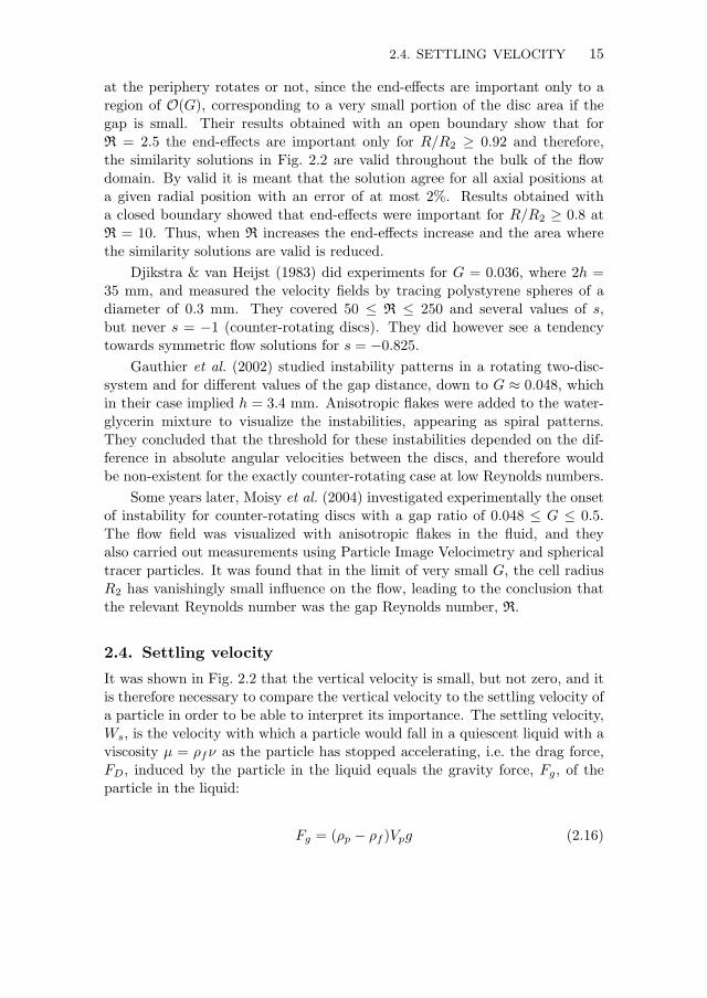
2.4. Settling velocity
It was shown in Fig. 2.2 that the vertical velocity is small, but not zero, and itis therefore necessary to compare the vertical velocity to the settling velocity ofa particle in order to be able to interpret its importance. The settling velocity,Ws, is the velocity with which a particle would fall in a quiescent liquid with aviscosity µ = ρfν as the particle has stopped accelerating, i.e. the drag force,FD, induced by the particle in the liquid equals the gravity force, Fg, of theparticle in the liquid:
Fg = (ρp − ρf )Vpg (2.16)
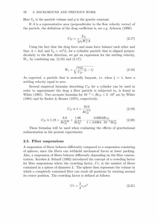
16 2. BACKGROUND AND PREVIOUS WORK
Here Vp is the particle volume and g is the gravity constant.If A is a representative area (perpendicular to the flow velocity vector) of
the particle, the definition of the drag coefficient is, see e.g. Acheson (1990):
CD =FD
12ρfW
2sA
(2.17)
Using the fact that the drag force and mass force balance each other andthat A = 2aL and Vp = πa2L, for a cylindric particle that is aligned perpen-dicularly to the flow direction, we get an expression for the settling velocity,Ws, by combining eqs. (2.16) and (2.17):
Ws =√πag
CD(ξ − 1) (2.18)
As expected, a particle that is neutrally buoyant, i.e. when ξ = 1, have asettling velocity equal to zero.
Several empirical formulas describing CD for a cylinder can be used inorder to approximate the drag a fiber particle is subjected to, is found inWhite (1991). Two accurate formulas for 10−4 < ReD < 2 · 105 are by White(1991) and by Sucker & Brauer (1975), respectively:
CD ≈ 1 +10.0
Re2/3D
(2.19)
CD ≈ 1.18 +6.8
Re0.89D
+1.96Re0.5D
− 0.0004ReD1 + 3.6364 · 10−7Re2D
(2.20)
These formulas will be used when evaluating the effects of gravitationalsedimentation in the present experiments.
2.5. Fiber suspensions
A suspension of fibers behaves differently compared to a suspension consistingof spheres, since the fibers can withhold mechanical forces at lower packing.Also, a suspension of fibers behaves differently depending on the fiber concen-tration. Kerekes & Schnell (1992) introduced the concept of a crowding factorfor fibre suspensions where the crowding factor, Cr, is the number of fiberscontained in a sphere of diameter L. The sphere then represents the volume inwhich a completely contained fiber can reach all positions by rotating aroundits center position. The crowding factor is defined as follows:
Cr =23cvα
2 (2.21)

2.6. ORIENTATION OF FIBERS IN SHEAR FLOW 17
Cr Characteristics< 1 Dilute suspension, rare collisions of fibers
1− 60 Semi-dilute suspension, frequent collisions of fibers> 60 Concentrated suspension, continuous contact between fibers
Table 2.2. Characterization of a fiber suspension flowregimes by the crowding factor, Cr, according to Kerekes &Schnell (1992).
where cv is the volume concentration of fibers and α is the aspect ratio of thefibers. Sometimes it is more convenient to start from the mass concentrationof the suspension, cm = mf/ml where mf is the mass of dry fibers and ml isthe mass of liquid. Equation (2.21) can then be rewritten, with σ being thecoarseness [mass/length] of the fibers:
Cr =π
6cm
L2
σ(2.22)
The level of collisions of fibers in a suspension, and thus the tendency toform flocs, can therefore be characterized by the crowding factor, as specifiedin table 2.2.
Moreover, the presence of fibers has rheological implications, which arebeyond the scope of the present thesis. The interested reader can find a reviewon this topic in Petrie (1999).
2.6. Orientation of fibers in shear flow
Consider a slender body or fiber, as sketched in Fig. 2.4, in a shear flow in theXY -plane. In this figure, Φ is the angle between the projection of the fiber inthe XY -plane and the X-axis, and β is the angle between the fiber and theZ-axis. The origin of the coordinate system is always at the center of the fiber,and hence, the coordinate system moves with the translation velocity of thefiber.
The equations of motion of a solitary ellipsoid suspended in an unboundedlaminar simple shear flow, as in Fig. 2.4 with the shear flow in the XY -plane,were first solved theoretically by Jeffery (1922), and therefore the orbits, inwhich the slender body will move are called Jeffery orbits. In the solutionby Jeffery (1922), the orbits are characterized by a constant C, where C = 0represents a rolling fiber with its long axis aligned with the Z-axis in Fig. 2.4.A large value of C corresponds to the angle β being close to 90, and hence thefiber is almost in the XY -plane. In Fig. 2.5(a) the trace of one end of the fiberis plotted for C =0.05, 0.25, 1 and 25, where C = 0.05 is the smallest orbit.

18 2. BACKGROUND AND PREVIOUS WORK
Figure 2.4. Definition of angles for a slender body that hasits center at the origin.
The orbits, except the rolling one, performs a flipping motion, since the angleΦ changes rapidly with time as soon as it deviates from the X-direction. Theevolution of Φ as a function of time is plotted in Fig. 2.5. For intermediateC-values, the orbit motion is referred to as a kayaking motion, since the fibermotion is similar to the motion of a kayak paddle. For the highest C-value,the motion is pure flipping when no walls are present. If a wall is presentand the end of the fiber touches it, the motion is modified and referred to aspole-vaulting.
Stover & Cohen (1990) observed neutrally buoyant rodlike particles withaspect ratio of α = 12 and suspended in a pressure-driven flow in a Hele-Shawcell, i.e. between two flat plates, with λ = 3, 6 and 20, and at low Reynoldsnumbers. Both the orientation and position of the particles were recorded inthree dimensions by combining pictures from two different cameras. It wasobserved that particles oriented close to their vorticity axis and placed lessthan L/2 from the wall, remained close to the wall and had a somewhat longerperiod of rotation than predicted by theory with no wall present. Furthermore,the flipping particles also had a longer period of rotation and were forced by theinteraction of the wall to a position of L/2 from the wall after a pole-vaultingmotion.
Later, Carlsson et al. (2007) carried out experimental studies of orientationof fibers suspended in shear flow near a wall. In this study, the fibers situatedclose to a smooth wall mostly oriented themselves perpendicularly to the flow,and fibers positioned more than L/2 from the wall were oriented in the directionof the flow.

2.6. ORIENTATION OF FIBERS IN SHEAR FLOW 19
(a)
(b)
Figure 2.5. In (a): Jeffery orbits for C = 0.05, 0.25, 1 and25. In (b): the angle Φ showing the flipping behavior of a fiberin shear flow.
Holm & Soderberg (2007) experimentally studied a laminar fiber suspen-sion flow down an inclined plane, and the fiber orientation was extracted. Fiberswere found to be mostly oriented perpendicularly to the flow direction near thewall. Moreover, it was found that the number of such fibers decreased as the
20 2. BACKGROUND AND PREVIOUS WORK
Figure 2.6. Sketch of rotating cylinders in linear shear flow.
fiber aspect ratio increased. Fibers far from the wall were mostly aligned inthe flow direction.
Slender bodies are here interpreted as fibers, which are the interest for thepapermaking industry, but slender bodies are also of interest to other researchareas, e.g. geology. Ventura et al. (1996) investigated the orientation of pla-gioclase crystals in high-viscosity lava flows. The lava flow is similar to a pipeflow and plagioclase are crystals with a blade shape and rectangular with anapproximate length-to-width ratio of 3.5 − 4. The investigation was carriedout by taking photos of thin sections of the solidified lava and analyzing thesepictures. It was found that the angle between the crystal and the ground inthe flow direction (corresponding to Φ in Fig. 2.4) was close to zero in theproximity of the lower boundary (the ground), and increased quickly with thedistance. This relationship was seen to an angle of approximately 40 beforea random distribution was seen for crystals in the middle between the groundand the upper boundary (crust). Near the crust, the angle between the crys-tal and the crust decreased as the distance between the crystal and the crustdecreased. Ventura et al. (1996) concluded that the crystal alignments couldbe used to identify different deformation zones in the lava flow and that thetextural features of the lava could be explained by the flow profile. However,it should be noted that a lava flow is complicated, e.g. the final deformationevent modifies the previous crystal alignment and the pressure increases in themiddle as the lava solidifies.
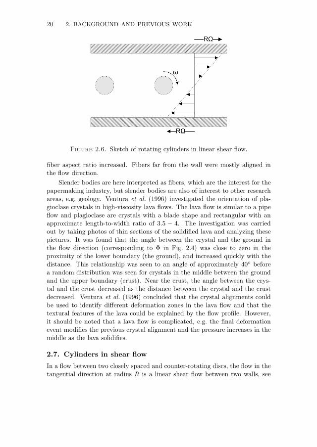
2.7. Cylinders in shear flow
In a flow between two closely spaced and counter-rotating discs, the flow in thetangential direction at radius R is a linear shear flow between two walls, see

2.7. CYLINDERS IN SHEAR FLOW 21
Fig. 2.6, where the upper and lower walls have the velocities RΩ and −RΩ,respectively. Radially aligned fibers can then be viewed as rotating cylinders,as illustrated in the figure. Studies can be found regarding one rotating cylinderin a linear shear flow, but the torque in the literature is not always zero, i.e.the cylinder is not necessarily rotating freely. Other properties to take intoconsideration is whether the flow is bounded by walls or not and how far awaythese walls are positioned. Also, if the flow is co- or counter-flowing and if thereare one or several cylinders and finally if the cylinders are neutrally buoyant(if not fixed) or not.
Zhao et al. (1998) studied a freely rotating and translating cylinder witha diameter d in a pipe flow in a 2D channel with a height of 2h = 10 d.A volume-based finite-element method was used and the results (consideringonly Z ≤ 0) showed that, for Rez = 2hU/ν = 1 (U is the mean velocity inthe channel), the lift was positive for Z/h < −0.7 but negative for other values(−0.7 < Z/h < 0), except in the middle of the channel Z/h = 0 where it alsowas zero. For increasing Reynolds numbers, up to 50, the zero lift point movedsomewhat closer to the wall.
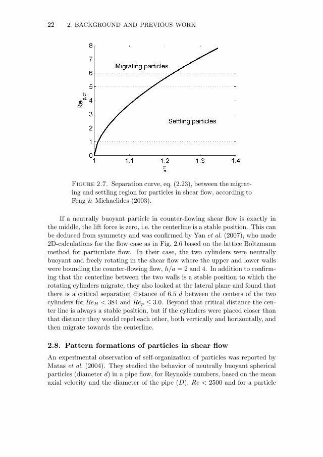
For particles heavier than the fluid, the gravity force have to be balanced bya lift force in order for the particles to find stable positions where their verticalvelocity is zero. This was studied, with cylindrical particles of diameter d in a2D co-flowing linear shear flow by Feng & Michaelides (2003) They used thelattice Boltzmann method and did calculations for particle Reynolds numbers0.5 ≤ Rep ≤ 5 and for density ratios 1.001 ≤ ξ ≤ 1.1. The channel used hada height of 10 d and a width of 20 d, and the shear rate was γ = UW /(2h).The upper wall moved with velocity UW and the lower wall was stationary.They calculated the equilibrium positions when both the lift created by theshear and by the proximity of the wall were balanced by the gravity force ofthe particle. If the gravity force was too large, the cylinders were not able tomigrate away from the wall but settled instead. A settled particle is definedas having a clearance of < 0.2 d to the lower wall. Feng & Michaelides (2003)proposed the following equation:
Rep,cr =584
(ξ − 1)0.59 (2.23)
in order to describe the curve separating the two regions of settling and migrat-ing particles. It is plotted in Fig. 2.7 for a larger range of ξ than investigatedin the study by Feng & Michaelides (2003). In this figure, it can be seen thatlighter particles, but still heavier than the fluid, need a smaller Rep in order toovercome its weight and start migrating. In their study it was also observedthat lighter particles migrates to a higher equilibrium position, compared toheavier particles.
22 2. BACKGROUND AND PREVIOUS WORK
Figure 2.7. Separation curve, eq. (2.23), between the migrat-ing and settling region for particles in shear flow, according toFeng & Michaelides (2003).
If a neutrally buoyant particle in counter-flowing shear flow is exactly inthe middle, the lift force is zero, i.e. the centerline is a stable position. This canbe deduced from symmetry and was confirmed by Yan et al. (2007), who made2D-calculations for the flow case as in Fig. 2.6 based on the lattice Boltzmannmethod for particulate flow. In their case, the two cylinders were neutrallybuoyant and freely rotating in the shear flow where the upper and lower wallswere bounding the counter-flowing flow, h/a = 2 and 4. In addition to confirm-ing that the centerline between the two walls is a stable position to which therotating cylinders migrate, they also looked at the lateral plane and found thatthere is a critical separation distance of 6.5 d between the centers of the twocylinders for ReH < 384 and Rep ≤ 3.0. Beyond that critical distance the cen-ter line is always a stable position, but if the cylinders were placed closer thanthat distance they would repel each other, both vertically and horizontally, andthen migrate towards the centerline.
2.8. Pattern formations of particles in shear flow
An experimental observation of self-organization of particles was reported byMatas et al. (2004). They studied the behavior of neutrally buoyant sphericalparticles (diameter d) in a pipe flow, for Reynolds numbers, based on the meanaxial velocity and the diameter of the pipe (D), Re < 2500 and for a particle

2.8. PATTERN FORMATIONS OF PARTICLES IN SHEAR FLOW 23
Reynolds number, Rep = Re(d/D)2, of approximately up to 10. By takingpictures of the flow and by identifying and counting the particles by eye, theyobserved long-lived trains of spheres aligned with the flow. The mean surfaceseparation distance between the particles decreased with increasing Rep. Thetrains could be very long and were observed to form at a position 0.6 timesthe radius of the pipe, known as the Segre-Silberberg equilibrium annulus, fordetails see Segre & Silberberg (1962).
Similar effects as those of Matas et al. (2004) has also been observed in anumerical simulation by Chun & Ladd (2006). They used a square duct flowin which they simulated neutrally buoyant spherical particles and their migra-tion, by using the lattice-Boltzmann method. The particle diameter was about1/10 of the channel dimension and trains were observed to form at equilib-rium positions if the suspension was dilute and if the Reynolds number, basedon the width of the channel and the mean velocity, was in the range 100 to1000. At higher Reynolds numbers the trains broke up and the particles mi-grated towards an equilibrium position in the middle (Re ∼ 1000) and formedclusters.
Di Carlo et al. (2007) investigated positioning of particles with different ge-ometries by doing experiments in laminar flow in microchannels, and unexpect-edly observed pattern formations both longitudinally (along the streamlines)in regular chains and rotationally for discoidal red blood cells. By changingthe symmetry of the channel, they then succeeded in ordering spherical parti-cles of diameter 9 µm with good accuracy in three spatial dimensions. Theyconcluded that the ordering was independent of particle density for their cases,0.85 < ξ < 1.35, and that the migration was due to lift forces on the parti-cles. The experiments of blood cells were done within a 50 µm square channel(width w and height H). For a Reynolds number of 60, based on the hydraulicdiameter (Dh = 2wH/(w+H)) and maximum velocity of the channel, the cellsformed trains at the bottom and top of the channel with their disc axis, aroundwhich they rotated, parallel to the wall. This motion would look somethinglike a rolling tyre on the ground.
Self-organization of particles is also found when a thermally convectingfluid interacts with particles, as Liu & Zhang (2008) have investigated by exper-iments in a Rayleigh-Benard convection cell. They observed a cyclic behaviorof particles reorganizing from one side of the convection cell to the other.

24
CHAPTER 3
Experimental set-up, methods and data evaluation
3.1. Experimental set-up
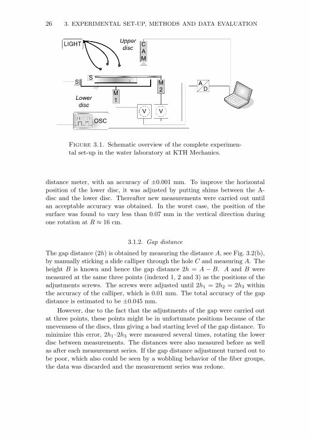
An experimental apparatus has been set up in order to study the flow of afiber suspension between two perfectly counter-rotating discs and a schematicoverview of the complete experimental set-up in the water laboratory at KTHMechanics is shown in Fig. 3.1. The laptop computer controls the camera(CAM) as well as the power generators (V), that give voltage to the motorsM1 and M2. Two sensors (S) read the speed of the discs and their signals aremonitored by the oscilloscope (OSC) and sent to the computer via an A/D-converter. The light source is also indicated, with its three-headed goosenecklamp.
3.1.1. The discs
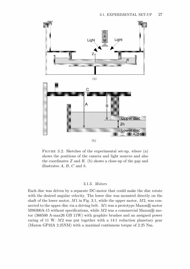
A sketch of the main parts of the experimental apparatus is shown in Fig. 3.2(a)with a close-up in Fig. 3.2(b). The apparatus consists of two flat and horizontaldiscs made of glass, mounted inside a cylindrical acrylic container with an innerdiameter of 45 cm. The upper disc is hanging under a flat 5 mm-thick aluminumring, which fits into the acrylic container and has an inner diameter of 26 cm.The aluminum ring is in turn hanging on the brim of the acrylic container bylong screws and hooks at three points and thus, there is no central axis goingthrough the gap between the discs.
The upper glass disc has a diameter of 30 cm and can be moved vertically byadjusting the long screws, in order to obtain the desired gap distance betweenthe discs. The lower disc is fixed vertically and at the edge of the lower disc,i.e. at radius 20 cm, there is a small wall to prevent the suspension (light grayarea in Fig. 3.2(a)) from escaping. Both discs have a thickness of 1 cm. Thesurface of the upper disc was measured with high-accuracy-shims (accuracy of0.001 mm) and was found to not vary more than 0.01 mm during one rotation.This variation was mostly due to a small play of the track, in which the discslides by the aid of a belt connected to the motor. The lower disc is fixedto another disc, denoted A-disc in Fig. 3.2(b) that is mounted on the centralaxis. The position of the surface of the lower disc was measured with a laser
25
26 3. EXPERIMENTAL SET-UP, METHODS AND DATA EVALUATION
Figure 3.1. Schematic overview of the complete experimen-tal set-up in the water laboratory at KTH Mechanics.
distance meter, with an accuracy of ±0.001 mm. To improve the horizontalposition of the lower disc, it was adjusted by putting shims between the A-disc and the lower disc. Thereafter new measurements were carried out untilan acceptable accuracy was obtained. In the worst case, the position of thesurface was found to vary less than 0.07 mm in the vertical direction duringone rotation at R ≈ 16 cm.
3.1.2. Gap distance
The gap distance (2h) is obtained by measuring the distance A, see Fig. 3.2(b),by manually sticking a slide calliper through the hole C and measuring A. Theheight B is known and hence the gap distance 2h = A − B. A and B weremeasured at the same three points (indexed 1, 2 and 3) as the positions of theadjustments screws. The screws were adjusted until 2h1 = 2h2 = 2h3 withinthe accuracy of the calliper, which is 0.01 mm. The total accuracy of the gapdistance is estimated to be ±0.045 mm.
However, due to the fact that the adjustments of the gap were carried outat three points, these points might be in unfortunate positions because of theunevenness of the discs, thus giving a bad starting level of the gap distance. Tominimize this error, 2h1–2h3 were measured several times, rotating the lowerdisc between measurements. The distances were also measured before as wellas after each measurement series. If the gap distance adjustment turned out tobe poor, which also could be seen by a wobbling behavior of the fiber groups,the data was discarded and the measurement series was redone.
3.1. EXPERIMENTAL SET-UP 27
(a)
(b)
Figure 3.2. Sketches of the experimental set-up, where (a)shows the positions of the camera and light sources and alsothe coordinates Z and R. (b) shows a close-up of the gap andillustrates A, B, C and h.
3.1.3. Motors
Each disc was driven by a separate DC-motor that could make the disc rotatewith the desired angular velocity. The lower disc was mounted directly on theshaft of the lower motor, M1 in Fig. 3.1, while the upper motor, M2, was con-nected to the upper disc via a driving belt. M1 was a prototype Maxonr motorM98300A-15 without specifications, while M2 was a commercial Maxonr mo-tor (366500 A-max26 GB 11W) with graphite brushes and an assigned powerrating of 11 W. M2 was put together with a 14:1 reduction planetary gear(Maxon GP32A 2.25NM) with a maximal continuous torque of 2.25 Nm.

28 3. EXPERIMENTAL SET-UP, METHODS AND DATA EVALUATION
3.1.4. Angular velocity control
The rotational velocity of each disc was measured with an optical system. Theside walls of the discs were striped black and white and two reflective objectsensors (Photologicr OPB715), S in Fig. 3.1, were used to obtain square wavesignals, generated by the stripes when the discs were rotating, from which theangular velocities were calculated.
The upper disc rotated counter clockwise and the lower one clockwise whenviewed from above, and the absolute values of the angular velocities were thesame for each measured case, with an accuracy of ±0.015 rad/s. This gave anaccuracy of 2% at the lowest speed, 0.75 rad/s. The angular velocities were setby the voltage generated by the power generators, which in turn were controlledby the laptop. Once the preset velocities were obtained, the camera was usedto obtain images.
3.1.5. Camera and light source
The CCD-camera (Basler PiA1900, 32 fps, 1080×1920, 8 bit/pixel) was mountedabove the discs and captured images of the fibers in the suspension through theupper glass disc. The captured area included the radius from approximately 3to 12 cm. The exposure time was set to 1 ms and for illumination a cold lightsource (Schott KL2500LCD) was used at 3000 − 3200 K equivalent tempera-ture. The light source had a three-headed gooseneck that made it possible toilluminate from three directions at the same time. The captured images weretransferred to a laptop computer.
3.1.6. Fiber suspension
The fibers in the suspension between the discs were white cellulose acetatefibers with a nominal length of L = 1 mm with small deviations from thisvalue. They were stiff, straight and had a density, ρp ≈ 1.3. The fiber lengthwas measured using the FiberMaster at Innventia AB (former STFI-Packforsk)where the mean length was measured to be 1.061 mm and where 91.6% of thefibers were in the length interval 0.9 ≤ L ≤ 1.2 mm. Also, the mean diameterwas measured to be d = 69.7µm for 88.2% of the fibers in the length interval0.5 < L < 1.5 mm.
Experiments with fibers of nominal length L = 0.5 mm and L = 2 mmwere also performed. These fibers have not been measured with FiberMaster,but were considered to have the same diameter and density as the 1 mm fibers,because they came from the same thread which was cut in different lengths.They were also supposed to have the same accuracy regarding their respectivelengths. The aspect ratios for the fibers L = 0.5 mm, L = 1 mm and L = 2 mmwere α = 7, 14 and 28, respectively.
3.2. EVALUATION TECHNIQUES 29
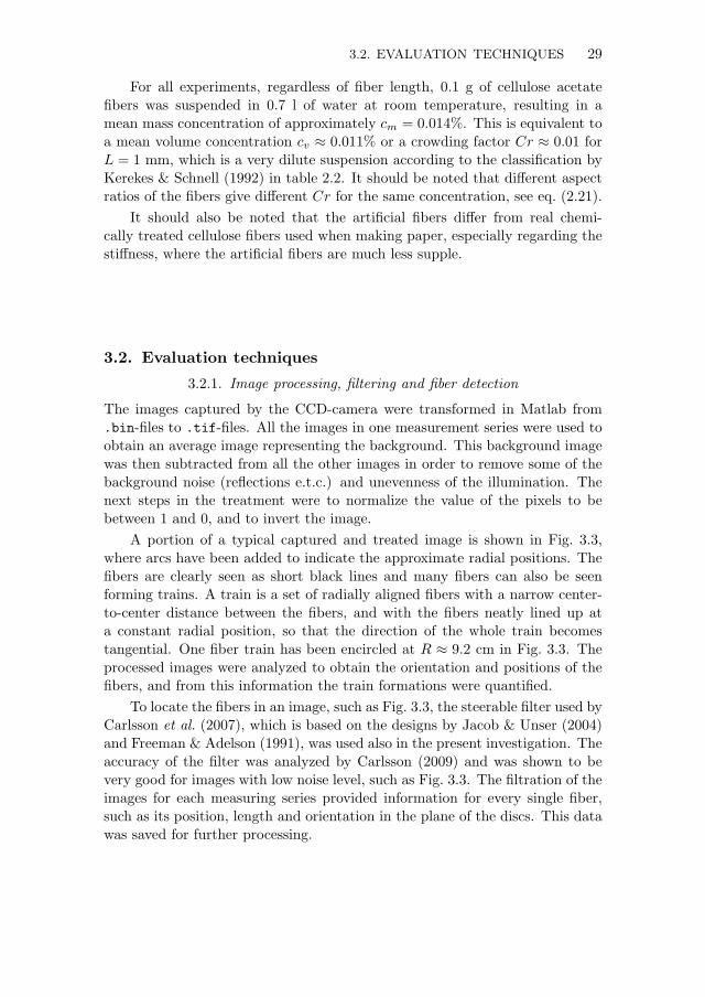
For all experiments, regardless of fiber length, 0.1 g of cellulose acetatefibers was suspended in 0.7 l of water at room temperature, resulting in amean mass concentration of approximately cm = 0.014%. This is equivalent toa mean volume concentration cv ≈ 0.011% or a crowding factor Cr ≈ 0.01 forL = 1 mm, which is a very dilute suspension according to the classification byKerekes & Schnell (1992) in table 2.2. It should be noted that different aspectratios of the fibers give different Cr for the same concentration, see eq. (2.21).
It should also be noted that the artificial fibers differ from real chemi-cally treated cellulose fibers used when making paper, especially regarding thestiffness, where the artificial fibers are much less supple.
3.2. Evaluation techniques
3.2.1. Image processing, filtering and fiber detection
The images captured by the CCD-camera were transformed in Matlab from.bin-files to .tif-files. All the images in one measurement series were used toobtain an average image representing the background. This background imagewas then subtracted from all the other images in order to remove some of thebackground noise (reflections e.t.c.) and unevenness of the illumination. Thenext steps in the treatment were to normalize the value of the pixels to bebetween 1 and 0, and to invert the image.
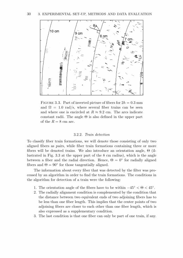
A portion of a typical captured and treated image is shown in Fig. 3.3,where arcs have been added to indicate the approximate radial positions. Thefibers are clearly seen as short black lines and many fibers can also be seenforming trains. A train is a set of radially aligned fibers with a narrow center-to-center distance between the fibers, and with the fibers neatly lined up ata constant radial position, so that the direction of the whole train becomestangential. One fiber train has been encircled at R ≈ 9.2 cm in Fig. 3.3. Theprocessed images were analyzed to obtain the orientation and positions of thefibers, and from this information the train formations were quantified.
To locate the fibers in an image, such as Fig. 3.3, the steerable filter used byCarlsson et al. (2007), which is based on the designs by Jacob & Unser (2004)and Freeman & Adelson (1991), was used also in the present investigation. Theaccuracy of the filter was analyzed by Carlsson (2009) and was shown to bevery good for images with low noise level, such as Fig. 3.3. The filtration of theimages for each measuring series provided information for every single fiber,such as its position, length and orientation in the plane of the discs. This datawas saved for further processing.
30 3. EXPERIMENTAL SET-UP, METHODS AND DATA EVALUATION
Figure 3.3. Part of inverted picture of fibers for 2h = 0.3 mmand Ω = 1.0 rad/s, where several fiber trains can be seenand where one is encircled at R ≈ 9.2 cm. The arcs indicateconstant radii. The angle Θ is also defined in the upper partof the R = 8 cm arc.
3.2.2. Train detection
To classify fiber train formations, we will denote those consisting of only twoaligned fibers as pairs, while fiber train formations containing three or morefibers will be denoted trains. We also introduce an orientation angle, Θ (il-lustrated in Fig. 3.3 at the upper part of the 8 cm radius), which is the anglebetween a fiber and the radial direction. Hence, Θ = 0 for radially alignedfibers and Θ = 90 for those tangentially aligned.
The information about every fiber that was detected by the filter was pro-cessed by an algorithm in order to find the train formations. The conditions inthe algorithm for detection of a train were the following:
1. The orientation angle of the fibers have to be within −45 < Θ < 45.2. The radially alignment condition is complemented by the condition that
the distance between two equivalent ends of two adjoining fibers has tobe less than one fiber length. This implies that the center points of twoadjoining fibers are closer to each other than one fiber length, which isalso expressed as a supplementary condition.
3. The last condition is that one fiber can only be part of one train, if any.

3.3. EXPERIMENTAL PROCEDURES AND PARAMETERS 31
To explain the algorithm figuratively, fibers belonging to a train are calledpassengers and fibers lying close to each other are called neighbors. To beginwith, the information about all the fibers detected in one image was consideredand all the relative distances were calculated. The fibers with neighboring fibersclose enough, in accordance with the conditions, were filtered out as possibletrain passengers, or candidates. The first passenger of a train, i.e. the fiber atone end of the train, must be a candidate with only one neighbor and whensuch a fiber is found, it is marked with a train identification number and thesearch for the rest of the passengers begins. The next step is to investigate theneighbors of this first passenger in order to see which fiber that is the closest oneand not being one already marked with a train identification number. Whenthe next passenger is found, it is marked with the same train identificationnumber as the first fiber and the algorithm focuses on the neighbors of thisnew passenger. One of its neighbors is evidently the first passenger in thetrain, but since it is already marked with a train identification number it willbe ignored. The algorithm then continues in the same way until the end ofthe train is reached, i.e. when no more unmarked neighbors exist. Informationabout the train, such as train identification number, center position, numberof fibers and mean and median distance between fibers, is saved. Thereafterthe algorithm looks for a new and unmarked first-passenger to the next train,which will be assigned a new train identification number.
The success rate of the algorithm to find the fiber trains is high, due to thegenerous conditions. The disadvantage of the generous conditions is the factthat short trains, with only a couple of fibers, should sometimes not have beenclassified as a train by eye, but are just fibers happening to be close to eachother in an almost-like-train formation. This effect is considerable for pairs,but smaller for trains containing three or more fibers. It is worth mentioningthat pairs were also detected and saved by the algorithm.
3.3. Experimental procedures and parameters
The camera was mounted and adjusted to capture an appropriate area of thedisc, that covered the radius from approximately 2–11 cm. The aim was to haveone radial line along the long centerline of the image, see Fig. 3.4. In order todo this calibration, a ruler was placed on the upper disc along a line with itszero position at the center of the disc. A picture was taken with the camera andthis image was imported to Matlab, where the positions (in pixels) of all visiblecentimeter markings of the ruler were recorded by hand, the number of pixelsper centimeter was calculated as well as the hub position. This procedure wascarried out every time the camera’s position was adjusted.
Long series of triplets of images were captured, where the time betweenstarts of triplets was 10 s and the time between pictures in one triplet was

32 3. EXPERIMENTAL SET-UP, METHODS AND DATA EVALUATION
Figure 3.4. Sketch of the camera’s area of coverage (grayarea) of the upper disc. The arrow indicates the direction ofthe ruler.
10 ms. For this study, the first image of each triplet is the one that has beenanalyzed. The reason for taking triplets was to get information about velocitiesof fibers and trains within a short range of time, but this has not yet beenperformed and is subject to future research.
Ω 2h Non-dim. numbersrad/s rpm mm d ReH R Reφ Rep G
min 0.75 7 0.1 1.4 9 0.01 0 0.25 0.0007max 2.50 24 0.9 12.9 540 0.5 1.1 · 105 3.9 0.006
Table 3.1. The maximal investigated ranges for the angularvelocity, gap distances, and the corresponding ranges for thenon-dimensional numbers.
The numbers of triplets taken for each case involving 0.5 mm fibers typi-cally were 100 or 150 triplets. For 1 mm fibers, which is the most thoroughlyinvestigated fiber length, typically 300 triplets were taken for each case. Fi-nally, typical numbers for L = 2 mm are 67 or 150 triplets. The maximalvariation of parameters are shown in table 3.1. The exact parameter variationsand numbers of triplets taken for each series are shown in tables in appendix A.The measurements were performed during a period of approximately 7 months.
Between the measurement series the fiber suspension was mixed in orderto achieve an even initial distribution of the fibers in the gap. The mixing

3.3. EXPERIMENTAL PROCEDURES AND PARAMETERS 33
procedure was performed by manually adjusting the rotating speeds of theupper and lower disc until the fiber distribution was uniform, as observed bythe eye. For smaller gap distances this took longer time than for larger gaps,where the fibers could move more freely.
Figure 3.5. General migration behavior of fibers.
The cases were not run in any specific order, but as one gap distance hadbeen set, all the cases for that gap were run. The order of the cases for thatgap was then alternated between high and low values of the angular velocity.The reason for this was the fact that fibers tended to gather at different radiiand the mixing process could somewhat be shortened by this procedure. Thegeneral migration behavior of the fibers depending on size of gap and magnitudeof angular velocity is sketched in Fig. 3.5. This behavior of the fibers can berelated to the radial velocity profile in Fig. 2.2 where the velocity is directedinward for vertical positions near the middle of the gap and directed outwardfor positions near the lower disc. It can be seen in Fig. 3.5 that for small gapsand/or higher angular velocities the fibers are positioned near the middle ofthe gap, since they are migrating inwards towards the hub of the discs, i.e. thesame direction as the radial velocity. For large gaps and/or lower velocitiesit can be deduced that the fibers are closer to the lower disc, since they areheavier than the fluid and because of the outward migration direction.
A captured series of 300 images took about 50 min to run if no problemsarose. However, it can be seen in the tables in appendix A, that some of theseries are shorter than others and the reasons for this are mainly three. Onebeing that problems with the camera-computer transfer occurred, which led toa stop of the capturing process. This was quite common for the first sets ofmeasurements series. Another reason is that the fibers in some cases, mostlythose of larger gap distances, were quickly transported inwards or outwardscausing either flocculation in the center, or fibers moving out of sight. At thesepoints it was not sensible to take long series. The third reason is that forsome cases, especially at high angular velocities and large gaps, no trains were

34 3. EXPERIMENTAL SET-UP, METHODS AND DATA EVALUATION
formed. As might be expected, analysis of the images series has been correctedaccording to the number of images taken, if pertinent.
3.4. Characteristics of the flow
With our maximal value of the gap ratio, G = 0.006, being half of the smallestgap ratio that Daily & Nece (1960) used, in their experiments to classify theflow, and with our maximum rotational Reynolds number Reφ ≈ 1.1 · 105,the flow will always belong to Regime I and thus be laminar according totable 2.1. The study by Gauthier et al. (2002), concerning instability patterns,also implies that the flow in our parameter domain should be laminar.
The qualitative behavior of the single-phase flow in the apparatus was alsoinvestigated with Iriodin1 added to water. For the investigated combinations ofangular velocities and gap distances, there were no instability patterns visible.The gap distance was increased beyond the investigated range, in order to see ifinstabilities occurred. The gap distance had to be increased to approximately3 mm for this to happen at high angular velocities. For small gaps turbulentflow was not achievable with the existing motors.
According to Brady & Durlofsky (1987), the edge-effects would only influ-ence an area of O(2h/R2), which would be very small in our case. It wouldalso be outside the camera view. The image reaches at most to R ≈ 0.8R2.Furthermore, the study by Szeri et al. (1983) shows that the infinite-disc solu-tions are valid for R/R2 < 0.7 for a relatively large gap ratio, G = 0.05. Also,according to Moisy et al. (2004), the influence of the disc radius, R2, is reducedwhen G decreases and is vanishingly small when G 1.
It can thus be established that the flow field, in absence of fibers, betweenthe two rotating discs is laminar, without edge-effects in the camera view andthat the single-phase flow follows the similarity solutions in section 2.2.
The vertical velocity w/RΩ in Fig. 2.2 is small, but must be compared tothe settling velocity in order to understand its importance. We choose a fiberpositioned perpendicularly to the settling direction, thus having a represen-tative area of 2aL, since such a fiber would have the lowest settling velocity.By iterating eq. (2.18) and eq. (2.20), we get a dimensionless settling velocityUs = U/(hΩ) of order O(101) − O(102), which is much larger than the verti-cal flow velocity, w/(hΩ) that is approximately of order O(10−2), see Fig. 2.2.Therefore, it can be concluded that for z > 0, the vertical velocity in the flowfield is not large enough (by several orders of magnitude) to overcome the set-tling velocity giving lift to fibers. For z < 0, w/(hΩ) and Us are both actingin the same direction, i.e. down towards the lower disc.
1Iriodin is here 120 Lustre Satin from Merck, consisting of small flakes that orient themselves
according to the flow and that can reflect light. They give an image of flow field structures.

3.5. A NOTE ON STATISTICAL RELIABILITY OF THE DATA 35
Figure 3.6. Number of fibers found per filtered image asfunction of clock time, for the case with gap distance 2h =0.2 mm and different angular velocities as indicated in the leg-end. Period 1 is the first 5 minutes of measurements, Period 3is the last 5 min for a full series of 300 triplets. Period 2 is thetime in between.
3.5. A note on statistical reliability of the data
As mentioned earlier, long series of images were captured even though thedistribution of the number of fibers in the gap became stabilized very quickly.By stabilization we do not imply that the number of fibers found remainsconstant, but that the number of fibers and their general behavior are fairlyconstant and only changes slowly with time.
Graphs showing the number of detected fibers in the first image of eachtriplet, as a function of clock time, can be seen in Fig. 3.6, where all thegraphs are for the case where 2h = 0.2 mm and the fiber length is L = 1 mm.Ignoring the high frequency oscillations for the time being, it can be seen thatif there are significant changes in the number of detected fibers, e.g. for thecurve where Ω = 1.25 rad/s, they take place in the beginning, and that thenumber of detected fibers then becomes approximately constant or only slowlychanging with time. If the concentration of fibers would be uniform, onlyabout 20 fibers would be in the field of view of the camera. If instead, the

36 3. EXPERIMENTAL SET-UP, METHODS AND DATA EVALUATION
fibers were evenly distributed right on the lower disc, such an idealized surfacemean concentration [fibers/m2] of fibers would imply about 630 fibers in viewof the camera. 630 fibers in the smallest gap implies a Cr ≈ 0.33 for thewhole volume, which still is a very dilute suspension according to table 2.2.It is relevant to look at the surface mean concentration since the fibers areheavier than the fluid and will settle, especially for low angular velocities. Thismost probable vertical position of the fibers near the lower disc was mentionedin section 3.3 when discussing the migration behavior. Therefore, it is notsurprising to see that the number of fibers in Fig. 3.6 for the lowest angularvelocity, Ω = 0.75 rad/s, stays at a high value around 700 identified fibers perimage, which can be linked to the surface mean concentration.
Now considering the rapid variations in Fig. 3.6, they are due to the factthat the surfaces of the discs are not exactly horizontal and thus makes thefibers favor a specific tangential position. This can be deduced by the factthat the peaks appear periodically and when a new image has been taken aftera number of full rotations. For example, there are exactly 10 full rotationsbetween the peaks for 0.75 rad/s and about 30 full rotations between peaks for1.75 rad/s, which are the two angular velocities with the largest rapid variationsin number of fibers found.
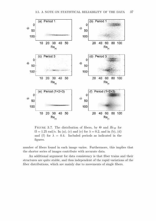
After analyzing the position and orientation of each fiber found, they couldbe sorted and summed up into a matrix, ReH × Θ. The values in the matrixwere then divided by the largest number in order to normalize the values tothe range 0–1. The resulting position-orientation matrix for the case whereΩ = 1.25 rad/s and λ = 0.2 is shown in Fig. 3.7(e) where black areas indicatewhere most fibers are and white ones where there are no fibers detected. Inthis figure, there are thus a lot of radially aligned fibers (Θ = 90), in the range20 < ReH < 55, whereas there are no tangentially aligned fibers.
Since this case (Ω = 1.25 rad/s and λ = 0.2) showed the largest declinein number of detected fibers in Fig. 3.6, position-orientation matrices for thefirst 30 images (Period 1) and the last 30 images (Period 3), respectively, wereextracted. They are showed in Fig. 3.7(a) and (c) and it can be seen that thedistributions do not vary significantly in appearance, even though the num-bers of fibers found are not the same. They are also similar to (e), where all300 images have been summed up to create the position-orientation matrix.
Figures (b), (d) and (f) show the same kind of distributions, but for thecase where λ = 0.4 and Ω = 1.25 rad/s. In these figures, both radially andalmost tangentially (Θ ≈ 0) aligned fibers are present. It can also be seen thatthe distributions for the different periods are, as in the previous case, similar.It can therefore be assumed that the results concerning fiber positions andorientations are not notably influenced by the initial effects when summarizingover a whole series of images. Thus, the data is consistent even though the
3.5. A NOTE ON STATISTICAL RELIABILITY OF THE DATA 37
Figure 3.7. The distribution of fibers, by Θ and ReH forΩ = 1.25 rad/s. In (a), (c) and (e) for λ = 0.2, and in (b), (d)and (f) for λ = 0.4. Included periods as indicated in thefigures.
number of fibers found in each image varies. Furthermore, this implies thatthe shorter series of images contribute with accurate data.
An additional argument for data consistency is that fiber trains and theirstructures are quite stable, and thus independent of the rapid variations of thefiber distributions, which are mainly due to movements of single fibers.

38

CHAPTER 4
Results and discussion
This chapter begins with a discussion about the flow as deduced from theparameter range, §4.1. Then the results concerning the orientation of individualfibers are presented in §4.2, followed by the behavior and occurrence of fibertrains in §4.3. In the latter section, qualitative observations concerning theforming, destruction and movement of trains are described. Furthermore, thelength of trains and their radial position are presented. Finally, the resultsfrom closer investigations of the structure of the trains are presented, §4.4-4.5.It should be noted that all results shown to this point are based on data fromfibers of with α = 14. The last section, §4.6, presents results obtained frominvestigations with α = 7, 14 and 28.
4.1. Flow conditions
As concluded in section 3.4 the flow field between the two discs is laminar, ifno fibers are present. In order to interpret and understand the results to come,it is worthwhile to discuss the interaction between fibers and such a flow field.
In section 3.4 in was also concluded that for z > 0, the vertical velocity,see Fig. 2.2(c), in the flow field is not large enough to overcome the settlingvelocity and to lift the fibers, and for z < 0, w/(hΩ) and the settling velocity(Us) are both acting in the same direction, i.e. down towards the lower disc.Thus, all vertical positions of the fibers, other than on the lower disc, are notdue to the vertical flow profile between the discs.
The velocity direction with the largest magnitude is the tangential one, seev/RΩ in Fig. 2.2(b), where the flow shows a linear shear profile for the relevantrange of the Reynolds number, i.e. 10−1 < R < 100.5.
The radial velocity is also important and the fibers are observed to migrateradially according to Fig. 3.5, which might be possible to explain by the verticalpositions of the fibers. The vertical positions are not possible to record directlyin the present set-up. Nevertheless, a comparison between the migration di-rection and the radial velocity profile indicates that for small gaps, when thefibers are almost stationary in the radial direction, the fibers are believed tobe located just below the middle z = 0, at the zero velocity point of u/RΩ, seeFig. 2.2(a). Their rotational speed, the wall effect and the fiber end-effects are
39

40 4. RESULTS AND DISCUSSION
very likely large enough to create a lift force that makes the particles migrate tothat point. Migration of particles was also investigated by Feng & Michaelides(2003), but in their study, the density ratio between particle and fluid was lessthan in our case, and using their formula for separation between migrating andsettling particles, eq. (2.23), we would in fact have a settling particle.
In addition to this, the tangential velocity of a fiber can be an indication ofits vertical position. It was seen in Fig. 2.2 that the tangential velocity profileis linear and a fiber following the fluid at a certain z-position would travelwith the corresponding velocity. Since we do not have quantitative data on thevertical position it is not possible to conclude this discussion at this point.
Still, for increasing gaps the lift force is not strong enough to transport theparticle to or above the lower zero velocity point, u = 0 in Fig. 2.2(a), and thefibers remain in the region below where the flow is directed outwards. Hence,outward migration of fibers is dominant for large gaps, which is seen in Fig. 3.5.
4.2. Orientation and position of fibers
The positions and orientations of the fibers depend on the angular velocities ofthe discs and the gap distance. Each detected fiber has a radial position, whichcan be translated to the Reynolds number, ReH , which includes the angularvelocity difference, ∆Ω, between the discs. The fiber also has an orientationand according to these two properties the fiber is placed in a matrix. All fibersfound, for one case, are added to the matrix at their appropriate position. Thematrix is then divided by the highest number in order to have values between 0and 1. This is now the distribution of fibers in the ReH–Θ plane. The accuracyof the angle was ±0.5 and the radial position of the fiber was determined withan accuracy of approximately ±0.4 mm.
Such distributions are seen in Figs. 4.1 and 4.2 for two different gaps andvarying Ω. In Fig. 4.3 results for Ω = 1.75 rad/s and varying gap distances areshown. In these figures, black areas indicate where most fibers are. It can beseen that the radially aligned fibers seemed to be dominating for approximatelyReH < 70 in the case where λ = 0.4, see Fig. 4.1. As the angular velocity isincreased the Reynolds number range increases, but high amount of radiallyaligned fibers (Θ = 0) around ReH = 60 remains. Furthermore, tangentiallyaligned fibers (Θ = 90) appear at higher ReH .
An interesting feature in Fig. 4.1 is that the tangentially aligned fibers tendto have an orientation angle, Θ, of either a little higher or a little lower than90 for the intermediate ReH , i.e. before ReH becomes high enough for all suchfibers to be almost exactly tangentially aligned, Θ = 90. This phenomenonproduces the rocket-like shape in the images for Ω = 1.75 rad/s and Ω =2.00 rad/s. For a larger gap, λ = 0.6 in Fig. 4.2, the rocket-like shape of the

4.2. ORIENTATION AND POSITION OF FIBERS 41
Figure 4.1. Position, ReH , and orientation, Θ, of fiberswhere black areas represent areas where most fibers are. λ =0.4 and Ω = (a) 0.75, (b) 1.0, (c) 1.25, (d) 1.5, (e) 1.75, (f)2.0, (g) 2.25 and (h) 2.5 rad/s.
distribution of the tangential fibers (Θ = 90) is less distinct, but is still thickertowards low ReH .
In Fig. 4.3, the effect of increasing gap distance is seen for Ω = 1.75 rad/s.Most fibers are radially aligned for the smallest gap, see (a), and as the gapincreases, more fibers are tangentially oriented.

42 4. RESULTS AND DISCUSSION
Figure 4.2. Position, ReH , and orientation, Θ, of fiberswhere black areas represent areas where most fibers are. λ =0.6 and Ω = (a) 0.75, (b) 1.0, (c) 1.25, (d) 1.5, (e) 1.75, (f) 2.0and (g) 2.25 rad/s.
The portion of radially and tangentially aligned fibers divided with the totalnumber of fibers found, versus the dimensionless gap λ is plotted in Figs. 4.4(a)and 4.4(b), respectively, for fibers with an aspect ratio α = 14. Radially alignedfibers are fibers with an orientation of Θ = 0 ± 5 and tangentially alignedfibers have Θ = 90 ± 5. Figure 4.4(a) shows that for small gaps, λ < 0.5, a
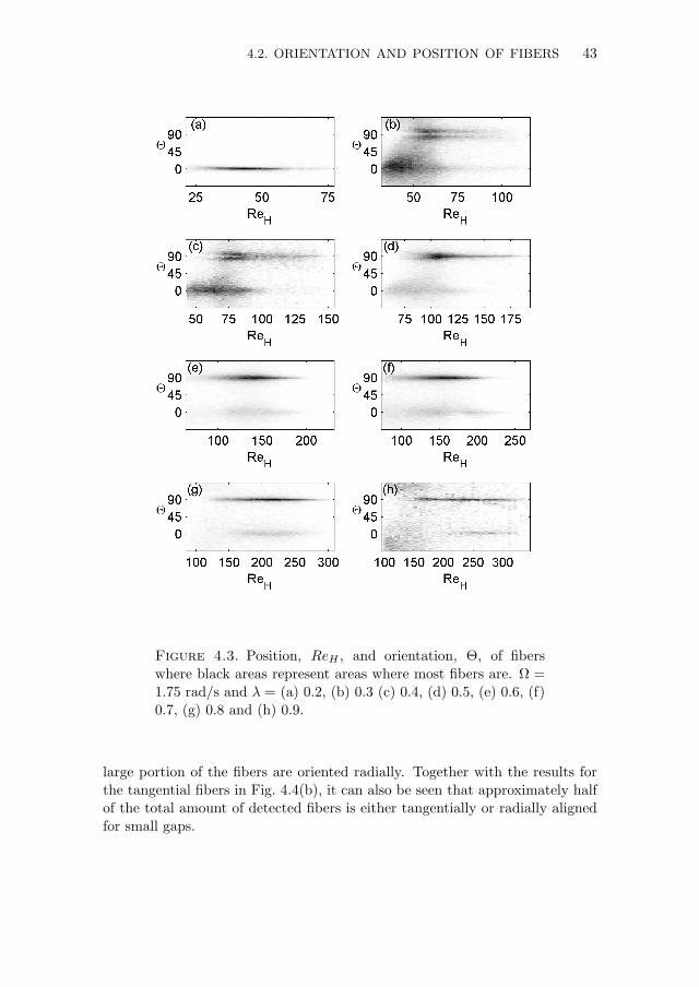
4.2. ORIENTATION AND POSITION OF FIBERS 43
Figure 4.3. Position, ReH , and orientation, Θ, of fiberswhere black areas represent areas where most fibers are. Ω =1.75 rad/s and λ = (a) 0.2, (b) 0.3 (c) 0.4, (d) 0.5, (e) 0.6, (f)0.7, (g) 0.8 and (h) 0.9.
large portion of the fibers are oriented radially. Together with the results forthe tangential fibers in Fig. 4.4(b), it can also be seen that approximately halfof the total amount of detected fibers is either tangentially or radially alignedfor small gaps.
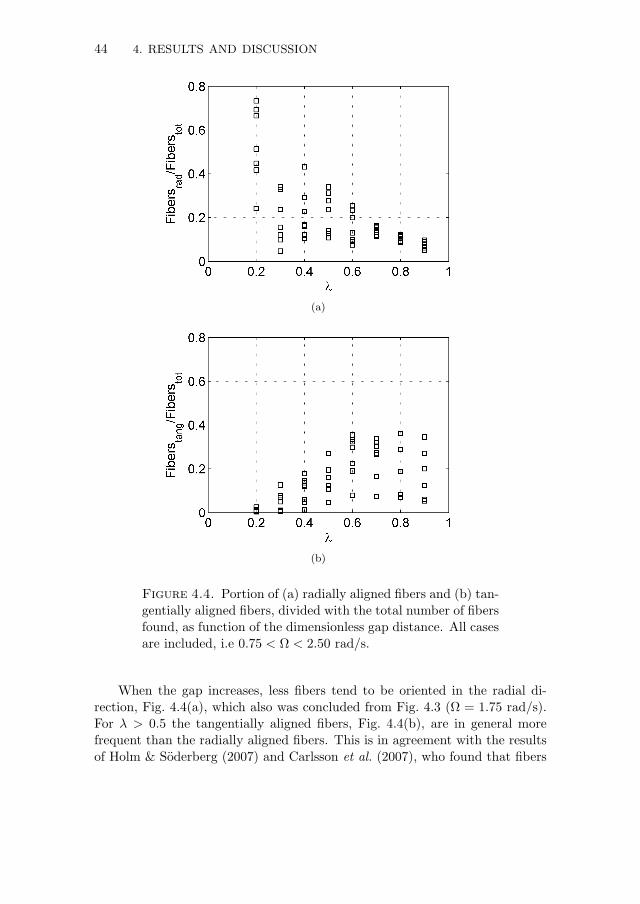
44 4. RESULTS AND DISCUSSION
(a)
(b)
Figure 4.4. Portion of (a) radially aligned fibers and (b) tan-gentially aligned fibers, divided with the total number of fibersfound, as function of the dimensionless gap distance. All casesare included, i.e 0.75 < Ω < 2.50 rad/s.
When the gap increases, less fibers tend to be oriented in the radial di-rection, Fig. 4.4(a), which also was concluded from Fig. 4.3 (Ω = 1.75 rad/s).For λ > 0.5 the tangentially aligned fibers, Fig. 4.4(b), are in general morefrequent than the radially aligned fibers. This is in agreement with the resultsof Holm & Soderberg (2007) and Carlsson et al. (2007), who found that fibers
4.3. BEHAVIOR AND OCCURRENCE OF FIBER TRAINS 45
were aligned with the flow direction for large distances from the wall (> L/2),and perpendicularly aligned with the flow direction close to the wall (< L/8).Since each disc is a wall, one would thus expect the majority of the fibers tobe perpendicular to the flow direction (fibers oriented radially in the presentexperiments) if
2h <L
8+L
8=L
4⇔ λ <
2hL< 0.25 (4.1)
This can be seen in Fig. 4.4, since it is at λ < 0.25 that the portion of radiallyaligned fibers is very large. The tangentially aligned fibers becomes dominatingwhen λ > 0.5.
Since the gap distance is less than one fiber length in all experimental cases,the fibers cannot flip around vertically, i.e. the pure flipping motion describedin section 2.6. Instead, they are mainly oriented in the horizontal plane, wherethey can do a resemblance of a kayaking motion of a solid ellipsoid in simpleshear flow or be rolling around their own axis. A selection of these motions(i.e. Jeffery orbits) were shown in Fig. 2.5(a).
The majority of the fibers appear to prefer either to be tangentially alignedor to be radially aligned in the horizontal plane. The fact that the radiallyaligned fibers rotate around their own axis can be seen by the eye for fibers thatare slightly bent. For tangentially aligned fibers, it has not been investigatedwhether the fibers rotate or not around their own axis, due to the difficulty ofvisualizing this. However, the shear of the radial velocity is non-zero, exceptat z = 0 and at the maxima of the velocity near each discs (see Fig. 2.2), andthat shear is probably strong enough to start rotating a tangentially alignedfiber around its own axis.
4.3. Behavior and occurrence of fiber trains
4.3.1. Qualitative observations
4.3.1a. Train forming and destruction. As already shown in Fig. 3.3, the fibersform regular patterns, here called fiber trains, in a similar manner as reportedfrom the experiments by Matas et al. (2004) for spheres in pipe flow and byDi Carlo et al. (2007) for spheres and oblate spheroids in pipe flow, and fromthe computations by Chun & Ladd (2006) for spheres in square pipe flow. Thephenomenon of pattern forming is similar, even though there are differencesregarding the geometries of the particles, density ratios, ambient flow fieldand the influence by walls. Fibers creating a fiber train are radially alignedand hence most fiber trains form when the portion of radially aligned fibers islarge. A qualitative observation of the fiber trains is that both the number oftrains and their lengths decrease as the gap increases. Also, there seem to bea preferred radial position where most of the trains form. When the angular

46 4. RESULTS AND DISCUSSION
(a) (b)
(c) (d)
Figure 4.5. Sequence of pictures showing the evolution of atrain crash and its reforming for Ω = 1.5 rad/s and λ = 0.2.The time between pictures is 0.5 s, and arrows are pointing atthe small fiber cluster causing the crash.
velocities are increased this radial position migrates a little outwards and thenbifurcates into two preferred radial positions for high velocities and large gaps.
For very small gaps, the trains are preferable formations for the fibers tobe in and they are very stable. As a consequence, there are few fast-movingfibers (tangentially aligned or doing a kayaking motion) that can collide witha train, causing it to be destroyed. If a train does get destroyed (crashes) in anarrow gap it quickly reforms into one or several (shorter) trains.
A sequence of pictures showing the evolution of a train crash is shownin Fig. 4.5. In this figure, trains are moving slightly with the lower disc, i.e.upwards. A small fiber cluster, at which the arrows point, causes the train tocrash and moves in the opposite direction, except between (c) and (d), wherethe cluster has moved in the same direction as the lower disc, hence having alower vertical position. In (a) the cluster touches a long train, and disturbsits side alignment. In (b), this disturbance has caused the train to completely
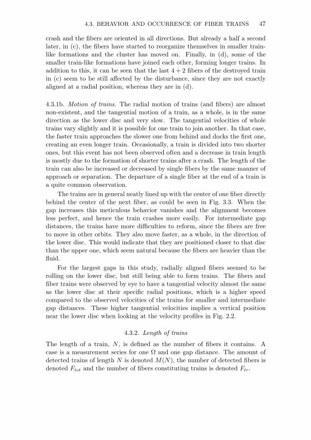
4.3. BEHAVIOR AND OCCURRENCE OF FIBER TRAINS 47
crash and the fibers are oriented in all directions. But already a half a secondlater, in (c), the fibers have started to reorganize themselves in smaller train-like formations and the cluster has moved on. Finally, in (d), some of thesmaller train-like formations have joined each other, forming longer trains. Inaddition to this, it can be seen that the last 4 + 2 fibers of the destroyed trainin (c) seem to be still affected by the disturbance, since they are not exactlyaligned at a radial position, whereas they are in (d).
4.3.1b. Motion of trains. The radial motion of trains (and fibers) are almostnon-existent, and the tangential motion of a train, as a whole, is in the samedirection as the lower disc and very slow. The tangential velocities of wholetrains vary slightly and it is possible for one train to join another. In that case,the faster train approaches the slower one from behind and docks the first one,creating an even longer train. Occasionally, a train is divided into two shorterones, but this event has not been observed often and a decrease in train lengthis mostly due to the formation of shorter trains after a crash. The length of thetrain can also be increased or decreased by single fibers by the same manner ofapproach or separation. The departure of a single fiber at the end of a train isa quite common observation.
The trains are in general neatly lined up with the center of one fiber directlybehind the center of the next fiber, as could be seen in Fig. 3.3. When thegap increases this meticulous behavior vanishes and the alignment becomesless perfect, and hence the train crashes more easily. For intermediate gapdistances, the trains have more difficulties to reform, since the fibers are freeto move in other orbits. They also move faster, as a whole, in the direction ofthe lower disc. This would indicate that they are positioned closer to that discthan the upper one, which seem natural because the fibers are heavier than thefluid.
For the largest gaps in this study, radially aligned fibers seemed to berolling on the lower disc, but still being able to form trains. The fibers andfiber trains were observed by eye to have a tangential velocity almost the sameas the lower disc at their specific radial positions, which is a higher speedcompared to the observed velocities of the trains for smaller and intermediategap distances. These higher tangential velocities implies a vertical positionnear the lower disc when looking at the velocity profiles in Fig. 2.2.
4.3.2. Length of trains
The length of a train, N , is defined as the number of fibers it contains. Acase is a measurement series for one Ω and one gap distance. The amount ofdetected trains of length N is denoted M(N), the number of detected fibers isdenoted Ftot and the number of fibers constituting trains is denoted Ftr.
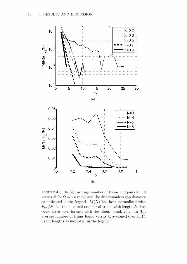
48 4. RESULTS AND DISCUSSION
(a)
(b)
Figure 4.6. In (a): average number of trains and pairs foundversus N for Ω = 1.5 rad/s and the dimensionless gap distanceas indicated in the legend. M(N) has been normalized withFtot/N , i.e. the maximal number of trains with length N thatcould have been formed with the fibers found, Ftot. In (b):average number of trains found versus λ, averaged over all Ω.Train lengths as indicated in the legend.

4.3. BEHAVIOR AND OCCURRENCE OF FIBER TRAINS 49
A plot of the number of pairs and trains, M(N ≥ 2), found versus the trainlength, N , for Ω = 1.5 rad/s and with a separate curve for each gap distance,is seen in Fig. 4.6(a). The horizontal axis has been limited to N ≤ 30 forbetter visualization and the number of pairs and trains on the vertical axis hasbeen normalized by the sum of fibers found for each gap and Ω = 1.5, dividedby N , i.e. normalization by the maximal number of N -trains that could havebeen formed with Ftot fibers. The curve over the number of pairs and trainssteepens as the gap distance increases which means that the maximum trainlength decreases when λ increases and that long trains only occur for smallergap distances.
A closer view at the number of trains, containing exactly N = 3, 4, 5and 8 fibers as function of the dimensionless gap can be seen in Fig. 4.6(b).The number of trains has been normalized by the sum of fibers found dividedby N , and averaged over all cases with equal λ. The number of N -fiber-trains decreases as the gap increases and shorter trains are more common forlarger gaps, which is in line with the qualitative observations in section 4.3.1.The decrease can be divided into a primary decrease at 0.2 < λ < 0.3 anda secondary decrease at 0.5 < λ < 0.6. For M(N = 3) a primary decreasecannot be seen and the reason for this may be that 3-fiber-trains at smallgaps are primarily waiting for another train, with which it may form a longertrain. The chance of joining another train and creating an even longer onedecreases as N increases. For larger gaps, 3-fiber-trains are primarily waitingto get destroyed, as are the longer trains. Hence, a secondary decrease can beseen for all N when λ > 0.5, which is when the tangentially aligned fibers aredominating, see section 4.2.
To quantify the maximum train lengths for our cases, a typical longesttrain length, L90, can be defined as the lowest L90 for which
L90∑N=3
pN > 0.90 (4.2)
where pN is the probability that an identified train has the length N and wherethe series pN is normalized so that
∞∑N=3
pN = 1 (4.3)
A plot of L90 versus λ is shown in Fig. 4.7 and it can be seen that for λ = 0.2there are lots of longer trains, which was also seen in Fig. 4.6(a). When thegap increases, L90 directly decreases to 4 − 6 fibers, and a final decrease hasoccurred at λ = 0.7 to 3− 4 fibers, which is the shortest possible train length.
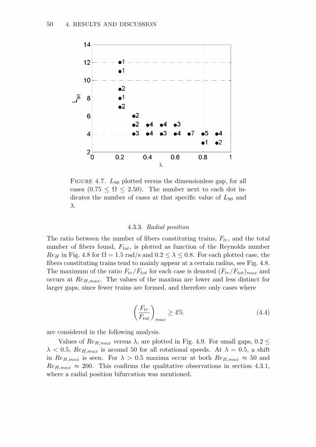
50 4. RESULTS AND DISCUSSION
Figure 4.7. L90 plotted versus the dimensionless gap, for allcases (0.75 ≤ Ω ≤ 2.50). The number next to each dot in-dicates the number of cases at that specific value of L90 andλ.
4.3.3. Radial position
The ratio between the number of fibers constituting trains, Ftr, and the totalnumber of fibers found, Ftot, is plotted as function of the Reynolds numberReH in Fig. 4.8 for Ω = 1.5 rad/s and 0.2 ≤ λ ≤ 0.8. For each plotted case, thefibers constituting trains tend to mainly appear at a certain radius, see Fig. 4.8.The maximum of the ratio Ftr/Ftot for each case is denoted (Ftr/Ftot)max andoccurs at ReH,max. The values of the maxima are lower and less distinct forlarger gaps, since fewer trains are formed, and therefore only cases where
(FtrFtot
)max
≥ 4% (4.4)
are considered in the following analysis.Values of ReH,max versus λ, are plotted in Fig. 4.9. For small gaps, 0.2 ≤
λ < 0.5, ReH,max is around 50 for all rotational speeds. At λ = 0.5, a shiftin ReH,max is seen. For λ > 0.5 maxima occur at both ReH,max ≈ 50 andReH,max ≈ 200. This confirms the qualitative observations in section 4.3.1,where a radial position bifurcation was mentioned.

4.4. DISTANCE BETWEEN FIBERS IN TRAINS 51
(a) (b)
(c) (d)
Figure 4.8. Ftr/Ftot versus ReH for Ω = 1.5 rad/s and (a)λ = 0.2, (b) λ = 0.4, (c) λ = 0.6 and (d) λ = 0.8.
However, since the discs in the present study are finite, large ReH cannotbe obtained for small gaps and there is a possibility that there might be asecond maximum of Ftr/Ftot at ReH ≈ 200 for small λ. The approximate limitof ReH is plotted as a dashed line in Fig. 4.9.
4.4. Distance between fibers in trains
The fibers in a train are lying next to each other and the distance from center-to-center point between fiber i and fiber i+ 1 is denoted δcc,i. We will presentthe mean distance between the surfaces of two adjacent fibers, denoted surfaceseparation distance, δss,i = δcc,i− d. Furthermore, δss is the mean value of the(N − 1) values of δss,i that exist for each train of length N :
δss =∑N−1i=1 δss,iN − 1
(4.5)
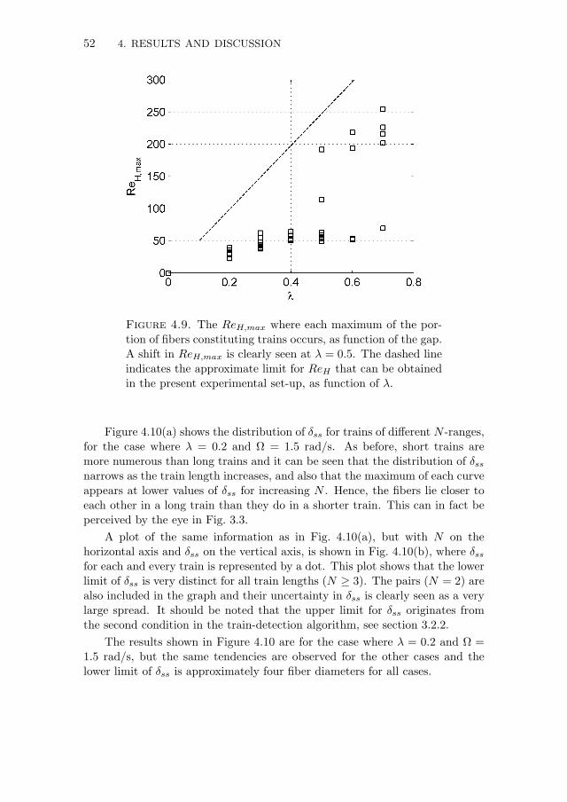
52 4. RESULTS AND DISCUSSION
Figure 4.9. The ReH,max where each maximum of the por-tion of fibers constituting trains occurs, as function of the gap.A shift in ReH,max is clearly seen at λ = 0.5. The dashed lineindicates the approximate limit for ReH that can be obtainedin the present experimental set-up, as function of λ.
Figure 4.10(a) shows the distribution of δss for trains of different N -ranges,for the case where λ = 0.2 and Ω = 1.5 rad/s. As before, short trains aremore numerous than long trains and it can be seen that the distribution of δssnarrows as the train length increases, and also that the maximum of each curveappears at lower values of δss for increasing N . Hence, the fibers lie closer toeach other in a long train than they do in a shorter train. This can in fact beperceived by the eye in Fig. 3.3.
A plot of the same information as in Fig. 4.10(a), but with N on thehorizontal axis and δss on the vertical axis, is shown in Fig. 4.10(b), where δssfor each and every train is represented by a dot. This plot shows that the lowerlimit of δss is very distinct for all train lengths (N ≥ 3). The pairs (N = 2) arealso included in the graph and their uncertainty in δss is clearly seen as a verylarge spread. It should be noted that the upper limit for δss originates fromthe second condition in the train-detection algorithm, see section 3.2.2.
The results shown in Figure 4.10 are for the case where λ = 0.2 and Ω =1.5 rad/s, but the same tendencies are observed for the other cases and thelower limit of δss is approximately four fiber diameters for all cases.
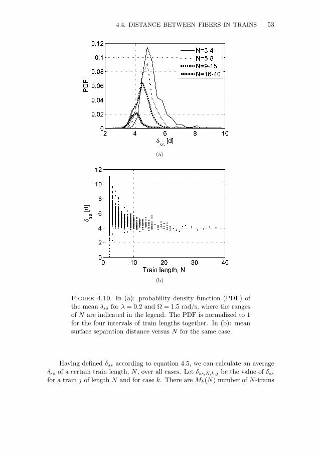
4.4. DISTANCE BETWEEN FIBERS IN TRAINS 53
(a)
(b)
Figure 4.10. In (a): probability density function (PDF) ofthe mean δss for λ = 0.2 and Ω = 1.5 rad/s, where the rangesof N are indicated in the legend. The PDF is normalized to 1for the four intervals of train lengths together. In (b): meansurface separation distance versus N for the same case.
Having defined δss according to equation 4.5, we can calculate an averageδss of a certain train length, N , over all cases. Let δss,N,k,j be the value of δssfor a train j of length N and for case k. There are Mk(N) number of N -trains
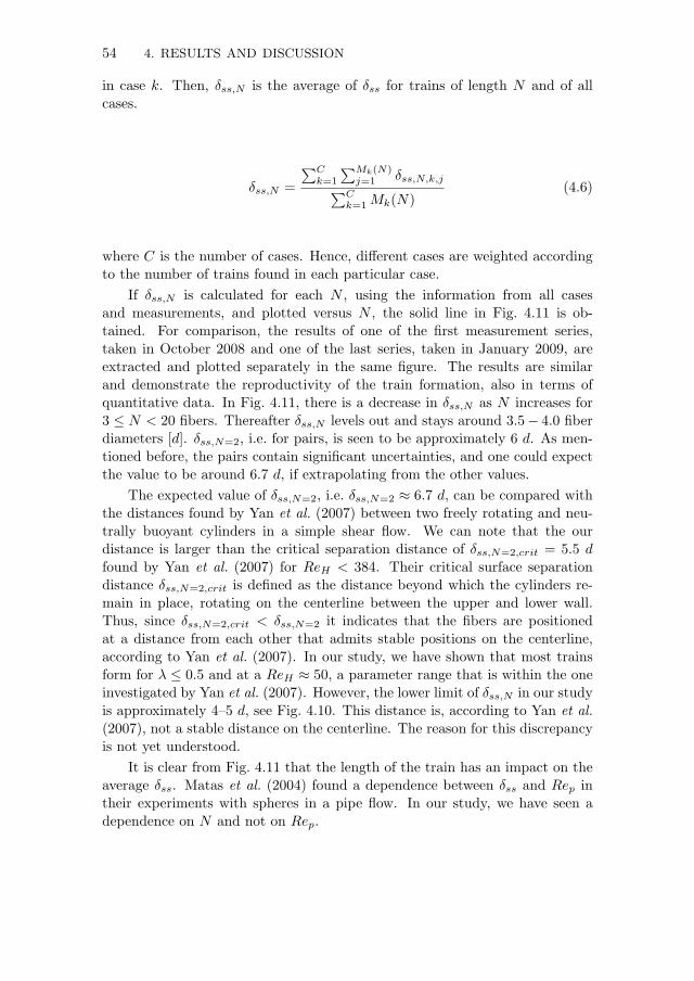
54 4. RESULTS AND DISCUSSION
in case k. Then, δss,N is the average of δss for trains of length N and of allcases.
δss,N =
∑Ck=1
∑Mk(N)j=1 δss,N,k,j∑C
k=1Mk(N)(4.6)
where C is the number of cases. Hence, different cases are weighted accordingto the number of trains found in each particular case.
If δss,N is calculated for each N , using the information from all casesand measurements, and plotted versus N , the solid line in Fig. 4.11 is ob-tained. For comparison, the results of one of the first measurement series,taken in October 2008 and one of the last series, taken in January 2009, areextracted and plotted separately in the same figure. The results are similarand demonstrate the reproductivity of the train formation, also in terms ofquantitative data. In Fig. 4.11, there is a decrease in δss,N as N increases for3 ≤ N < 20 fibers. Thereafter δss,N levels out and stays around 3.5− 4.0 fiberdiameters [d]. δss,N=2, i.e. for pairs, is seen to be approximately 6 d. As men-tioned before, the pairs contain significant uncertainties, and one could expectthe value to be around 6.7 d, if extrapolating from the other values.
The expected value of δss,N=2, i.e. δss,N=2 ≈ 6.7 d, can be compared withthe distances found by Yan et al. (2007) between two freely rotating and neu-trally buoyant cylinders in a simple shear flow. We can note that the ourdistance is larger than the critical separation distance of δss,N=2,crit = 5.5 dfound by Yan et al. (2007) for ReH < 384. Their critical surface separationdistance δss,N=2,crit is defined as the distance beyond which the cylinders re-main in place, rotating on the centerline between the upper and lower wall.Thus, since δss,N=2,crit < δss,N=2 it indicates that the fibers are positionedat a distance from each other that admits stable positions on the centerline,according to Yan et al. (2007). In our study, we have shown that most trainsform for λ ≤ 0.5 and at a ReH ≈ 50, a parameter range that is within the oneinvestigated by Yan et al. (2007). However, the lower limit of δss,N in our studyis approximately 4–5 d, see Fig. 4.10. This distance is, according to Yan et al.(2007), not a stable distance on the centerline. The reason for this discrepancyis not yet understood.
It is clear from Fig. 4.11 that the length of the train has an impact on theaverage δss. Matas et al. (2004) found a dependence between δss and Rep intheir experiments with spheres in a pipe flow. In our study, we have seen adependence on N and not on Rep.
4.5. ANGLE DEVIATION OF FIBERS IN TRAINS 55
Figure 4.11. The average surface separation distance for allcases with L = 1 mm versus N ≥ 2. The extracted results ofmeasurements taken in October 2008 and in January 2009 arealso plotted as separate curves.
4.5. Angle deviation of fibers in trains
As explained before in section 3.2.2, the condition for the angle deviation fromthe radial direction is set very generously in the algorithm for finding trains.The reason for this is to be sure to find fibers that might be part of a train.The candidate fibers of course have to be more numerous than the actualfibers belonging to trains. The algorithm described in section 3.2.2 searches forfiber train structures among the candidate fibers and the rest of the fibers arediscarded.
Figure 4.12 shows the distribution of orientation for the fibers found intrains for different ranges of N , where the sum of the distributions has beennormalized to 1. It is seen that fibers, identified as being passengers in a train,only deviate a few degrees from the radial direction. A fiber with a largedeviation is in most cases a fiber at one end of the train, thus in the process ofleaving or joining the train. This explains the large spread for shorter trains,where the end fibers constitute a large portion of the whole train.
An interesting feature in Fig. 4.12 is that the peaks of the PDF’s are notexactly at Θ = 0 but at higher values.

56 4. RESULTS AND DISCUSSION
Figure 4.12. Probability density function (PDF) of the an-gle deviation from the radial direction for λ = 0.2 and Ω =1.5 rad/s. Different ranges of train lengths are indicated in thelegend. The PDF is normalized to 1 for the four graphs to-gether.
4.6. Effect of fiber length
As mentioned earlier, two other fiber lengths (0.5 mm and 2 mm) with aspectratios α = 7 and α = 28, respectively, have been investigated. Here, the resultsof those will be compared to the results for α = 14 (L = 1 mm). This sectionwill highlight some interesting observations and results, related to fiber lengthvariation.
4.6.1. General observations
The general migration behavior, described in section 4.1, was modified accord-ing to Fig. 4.13 when the fiber aspect ratio changed. Fibers with lower aspectratio tend to migrate inwards to a larger extent, thus moving the border linebetween the two areas (i.e. outward and inward migration) down and to theleft. This implies that the fibers of lower aspect ratio, to a larger extent, are po-sitioned at z-values where the radial velocity is directed inward, see Fig. 2.2(a).Thus, the fibers experience a stronger lift force, possibly due to fiber end-effects.
The opposite migration behavior was seen for fibers with a higher aspectratio, which explains Fig. 4.13 for all three fiber lengths.

4.6. EFFECT OF FIBER LENGTH 57
Figure 4.13. General migration behavior of fibers of differentaspect ratios.
4.6.2. Ability to form trains
The shorter fibers required a smaller gap distance to form long trains, whichis consistent with the results of e.g. Carlsson et al. (2007) where the fibersmainly orient themselves perpendicularly to the flow if their center is locatedless than L/8 from the wall. It was seen that the shorter fibers formed trainswhen λ = 0.5 or less. The second condition in the algorithm for finding trains,described in section 3.2.2, were modified for the 0.5 mm fibers, where thedistances between two neighboring fibers and their ends were extended to 1.5 L.The reason for this is that δcc became too close to the value of L and fibersshould not be discarded as train passenger because of their length.
For the longer 2 mm fibers a new difficulty arose because of the fact thatthey were not completely straight, but often a little bent. Bent fibers easilycaused its own train or the train they were joining to crash since the fibers arerotating, and therefore there were few long trains for long fibers.
4.6.3. Surface separation distance
Calculations for the average surface separation distance, δss,N , were done forthe shorter and longer fiber lengths and the results can be seen in Fig. 4.14together with the results for α = 14. The results for pairs have been omittedbecause of the large errors of those results. The trend of decreasing δss,N forincreasing N can be seen for all fiber lengths, and it is interesting to see thatthe graphs for α = 14 and α = 28 almost coincide, but that the graph for theshorter fibers is moved downward to smaller δss,N , still having the same slope.This implies that for α < 14, end-effects and 3D effects become important andlead to shorter δss,N . A typical case where 3D effects cannot be neglected istrain forming of spheres. For such a case, Matas et al. (2004) found that thesurface separation distance was much shorter (0.5–3.5 d). For α = 7 the δss,N=2
is extrapolated to be approximately 5.5 d (i.e. δcc = 6.5 d), which is the value
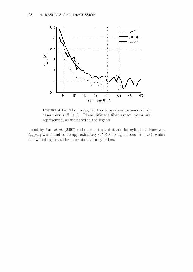
58 4. RESULTS AND DISCUSSION
Figure 4.14. The average surface separation distance for allcases versus N ≥ 3. Three different fiber aspect ratios arerepresented, as indicated in the legend.
found by Yan et al. (2007) to be the critical distance for cylinders. However,δss,N=2 was found to be approximately 6.5 d for longer fibers (α = 28), whichone would expect to be more similar to cylinders.
CHAPTER 5
Conclusions and outlook
The behavior of fibers suspended in a liquid flow between two flat and counter-rotating discs has been studied experimentally. The fibers had aspect ratiosα = 7, 14 and 28. The investigated range of the dimensionless gap distance,λ, between the discs was 0.2 ≤ λ ≤ 0.9 and the gap Reynolds number rangewas 9 < ReH < 540. The position and orientation of fibers in the plane ofthe discs were measured. Train formations, i.e. self-organization of a set ofradially oriented fibers at a constant radial position, with short fiber-to-fiberdistance in between, were observed to be a common feature in this set-up. Thebehavior, occurrence and structure of these train formations have been studiedand discussed.
Train formations require fibers to be aligned in the radial direction and ithas been observed that a larger portion of the fibers are radially aligned forgaps less than half of a fiber length. Most trains were also formed at smallgaps, with exceptionally long ones (up to 70 fibers) for a dimensionless gap ofλ = 0.2.
The surface separation distance, δss,N , between two adjacent fibers in atrain decreases as the length of the train, N , increases, i.e contains more fibers.The surface separation distance for a pair of α = 14 fibers is extrapolated toapproximately 6.7 fiber diameters. The distance decreases with increasing trainlength to around 4 fiber diameters for trains of approximately 20 fibers. Theresults for fibers with α = 28 were approximately the same, though the amountof data was less, and δss,N=2 was extrapolated to approximately 6.5 d.
The surface separation distance for fibers with α = 7 were found to besmaller for all values of N , compared to δss,N for longer fibers. Pairs of theshorter fibers have δss,N=2 ≈ 5.5 d. However, the surface separation distancedecreases with the same slope as the other fiber lengths with increasing N .
The results for a pair of fibers are in agreement with Yan et al. (2007), whofound that if δss ≥ 5.5 d between cylinders in a 2D flow, then the cylinders willremain in their positions.
59

60 5. CONCLUSIONS AND OUTLOOK
As mentioned in the beginning this study is the first undertaking in aneffort aimed at understanding what happens inside a refiner, used in the pa-permaking process. We have seen several interesting features, which deservemore attention and that will be investigated further, e.g. the velocities of wholetrains in an effort of determining their vertical positions. The work will thencontinue according to the strategy in section 1.2 with a more complex geometryof the experimental set-up, where it will be possible to have a throughflow offiber suspension and/or bars and grooves on the surfaces of the discs.

Acknowledgements
This project has been financially supported by the Swedish Energy Agency(Energimyndigheten) and is greatly acknowledged. Bengt Ingestroms stipendie-fond is also acknowledged for funding participation at international conferences.
I would like to thank my supervisors Daniel Soderberg and Fredrik Lundell forsupport and guidance.
I would also like to thank my colleagues at the Department of Mechanics,who have supported me and who create a good working atmosphere. Amongthese, I would like to mention Fredrik, Fritz, Goran, Ingunn, Kim, Lisa, Monika,Olle, Ramis and Shiho. Thanks also to my office mate Gabriele Bellani forpatience and good laughs.
Moreover, I would like to thank the people at Innventia AB, who kindlyhave supported me.
Huge thanks to my brother Mikael Ahlberg for enlightening me on many com-puter mysteries and for always being supportive. Finally, I very much thankmy friends and family for love and encouragement.
61

62
References
Abrahamson, H. 2008 Flytande kristaller smorjer battre an olja. News item in Ny
Teknik, 4 November 2008.
Acheson, D. J. 1990 Elementary Fluid Dynamics. Oxford University Press Inc., New
York.
Brady, J. F. & Durlofsky, L. 1987 On rotating disk flow. Journal of Fluid Me-
chanics 175, 363–394.
Carlsson, A. 2009 Near wall fibre orientation in flowing suspensions. PhD thesis,
Royal Institute of Technology, KTH Mechanics, Stockholm, Sweden.
Carlsson, A., Lundell, F. & Soderberg, L. D. 2007 Fibre orientation control re-
lated to papermaking. Journal of Fluids Engineering, Transactions of the ASME
129, 457–465.
Chun, B. & Ladd, A. J. C. 2006 Inertial migration of neutrally bouyant particles
in a square duct: An investigation of multiple equilibrium positions. Physics of
fluids 18, 031704.
Daily, J. W. & Nece, R. E. 1960 Chamber dimension effects on induced flow and
frictional resistance of enclosed rotating disks. Journal of Basic Engineering 82,
217–232.
Di Carlo, D., Irimia, D., Tompkins, R. G. & Toner, M. 2007 Continuous inertial
focusing, ordering, and separation of particles in microchannels. PNAS 104,
18892–18897.
Djikstra, D. & van Heijst, G. J. F. 1983 The flow between two finite rotating
disks enclosed by a cylinder. Journal of Fluid Mechanics 128, 123–154.
Feng, Z.-G. & Michaelides, E. E. 2003 Equilibrium position for a particle in a
horizontal shear flow. International Journal of Multiphase Flow 29, 943–957.
Fox, T. S., Brodkey, R. S. & Nissan, A. H. 1979 High-speed photography of
stock transport in a disk refiner. Tappi 62, 55–58.
Freeman, W. T. & Adelson, E. H. 1991 The design and use of steerable filters.
IEEE T. Pattern Anal. 13, 891–906.
Gauthier, G., Gondret, P., Moisy, F. & Rabaud, M. 2002 Instabilities in the
flow between co- and counter-rotating disks. Journal of Fluid Mechanics 473,
1–21.
63
64 REFERENCES
Greenspan, H. P. 1990 The Theory of Rotating Fluids. Breukelen Press, MA, USA.
Hoffman, G. H. 1974 Extension of perturbation series by computer: Viscous flow
between two infinite rotating discs. Journal of Comp. Phys. 16, 240–258.
Holm, R. & Soderberg, D. 2007 Shear influence on fibre orientation. Rheologica
Acta 46, 721–729.
Jacob, M. & Unser, M. 2004 Design of steerable filters for feature detection using
canny-like criteria. IEEE T. Pattern Anal. 26, 1007–1019.
Jeffery, G. B. 1922 The motion of ellipsoidal particles immersed in a viscous fluid.
Proc. Roy. Soc. London A 102, 161–179.
von Karman, T. 1921 Uber laminare und turbulente Reibung. Z. angew. Math.
Mech. 1, 233–251.
Kerekes, R. J. & Schnell, C. 1992 Characterization of fibre flocculation regimes
by a crowding factor. Journal of Pulp and Paper Science 18, 32–38.
Koskenhely, K., Ammala, A., Jokinen, H. & Paulapuro, H. 2005 Refining char-
acteristics of softwood fibre fractions. In 13th Fundamental Research Symposium,
Cambridge.
Liu, B. & Zhang, J. 2008 Self-induced cyclic reorganization of free bodies through
thermal convection. Physical Review Letters 100, 244501.
Matas, J.-P., Glezer, V. & Guazzelli, E. 2004 Trains of particles in finite
Reynolds-number pipe flow. Physics of Fluids 16, 4192–4195.
Moisy, F., Doar, O., Pasutto, T., Daub, O. & Rabaud, M. 2004 Experimental
and numerical study of the shear layer instability between two counter-rotating
disks. Journal of Fluid Mechanics 507, 175–202.
Norman, B. & Fellers, C. 1998 Pappersteknik . Institutionen for Pappersteknik,
KTH, Stockholm.
Petrie, C. 1999 The rheology of fibre suspensions. Journal of Non-Newtonian Fluid
Mechanics 87, 369–402.
Segre, G. & Silberberg, A. 1962 Behavior of macroscopic rigid spheres in poiseuille
flow part 2. Experimental results and interpretation. Journal of Fluid Mechanics
14, 136–157.
Stover, C. A. & Cohen, C. 1990 The motion of rodlike particles in the pressure-
driven flow between two flat plates. Rheologica Acta 29, 192–203.
Sucker, D. & Brauer, H. 1975 Fluiddynamik bei quer angestromten Zylindern.
Warme- und Stoffubertragung 8, 149–158.
Szeri, A. Z., Schneider, S. J., Labbe, F. & Kaufman, H. N. 1983 Flow between
rotating disks. part 1. basic flow. Journal of Fluid Mechanics 134, 103–131.
Ventura, G., Rosa, R. D., Colletta, E. & Mazzuoli, R. 1996 Deformation
patterns in high-viscosity lava flow inferred from the crystal preferred orientation
and imbrication structures: an example from Salina (Aeolian Islands, southern
Tyrrhenian Sea, Italy). Bull Volcanol 57, 555–562.
Weideman, J. A. C. & Reddy, S. C. 2000 A matlab differentiation matrix suite.
ACM Transactions on Mathematical Software 26, 465–519.
White, F. M. 1991 Viscous Fluid Flow . McGraw-Hill Inc.

REFERENCES 65
Yan, Y., Morris, J. F. & Koplik, J. 2007 Hydrodynamic interaction of two par-
ticles in confined linear shear flow at finite Reynolds number. Physics of fluids
19 (113305).
Zhao, Y., Sharp, M. K. & James, K. 1998 Finite-element analysis of transverse
lift on circular cylinder in 2d channel flow. Journal of Engineering Mechanics
124, 1152–1164.

66

APPENDIX A
Measurement data
Tables over the number of triplets for each measurement series, with theiridentification numbers indicated in the captions. The measurements were takenin the water laboratory at KTH, Stockholm, over a period of approximately7 months, from October 2008 to April 2009.
67

68 A. MEASUREMENT DATA
gap [mm]→ 0.9 0.8 0.7 0.6 0.5 0.4 0.3 0.2 0.1Ω [rad/s]↓
2.502.25 100 50 50 502.001.75 100 100 100 100 100 1501.50 150 150 150 150 80/150 801.25 100 150 50 150 150 150/1501.00 150 150 150 150 80/1500.75 100 150 150 150 150 80/150
Table A.1. Number of triplets taken for 0.5 mm fibers (seriesnos. 05mm0902 and 05mm0903). 10 s between triplets and1 ms between pictures in one triplet.
gap [mm]→ 0.9 0.8 0.7 0.6 0.5 0.4 0.3 0.2 0.1Ω [rad/s]↓
2.502.25 300 200 37 2002.00 300 300 263 2001.75 300 300 300 200 34 241.50 300 300 300 300 56 100 481.25 300 300 300 200 100 100 481.00 300 200 160 300 100 100 820.75 300 300 300 200 49 100
Table A.2. Number of triplets taken for 1 mm fibers (seriesno. 1mm1008). 10 s between triplets and 1 ms between picturesin one triplet.

A. MEASUREMENT DATA 69
gap [mm]→ 0.9 0.8 0.7 0.6 0.5 0.4 0.3 0.2 0.1Ω [rad/s]↓
2.50 1502.25 200 300 300 300 300 2372.00 250 300 300 300 300 300 300 3001.75 300 300 300 300 300 300 300 2791.50 300 300 300 300 300 300 300 3001.25 300 300 300 300 300 300 300 3001.00 300 300 300 300 300 300 300 3000.75 300 300 300 300 300 300 300 300
Table A.3. Number of triplets taken for 1 mm fibers (seriesno. 1mm0901). 10 s between triplets and 1 ms between picturesin one triplet.
gap [mm]→ 0.9 0.8 0.7 0.6 0.5 0.4 0.3 0.2 0.1Ω [rad/s]↓
2.50 672.25 67 67 67 672.00 150 150 1501.75 67 150 67 150 67 150 671.50 150 150 67 150 671.25 67 150 67 150 67 150 671.00 150 150 150 670.75 67 150 67 150 67 150 67
Table A.4. Number of triplets taken for 2 mm fibers (seriesnos. 2mm0902 and 2mm0904). 10 s between triplets and 1 msbetween pictures in one triplet.

70

APPENDIX B
Position-orientations pictures
Pictures over the positions and orientations of fibers (α = 14) for gaps 0.2 ≤λ ≤ 0.9 and angular velocities 0.75 ≤ Ω ≤ 2.50. The pictures for λ = 0.4 andλ = 0.6 were shown in section 4.2, but are also included here in order to havethe complete set of figures in the appendix.
71

72 B. POSITION-ORIENTATIONS PICTURES
Figure B.1. Positions and orientation distribution of fibersfor λ = 0.2 and Ω = (a) 0.75, (b) 1.0, (c) 1.25, (d) 1.5, (e)1.75, (f) 2.0 and (g) 2.25 rad/s.
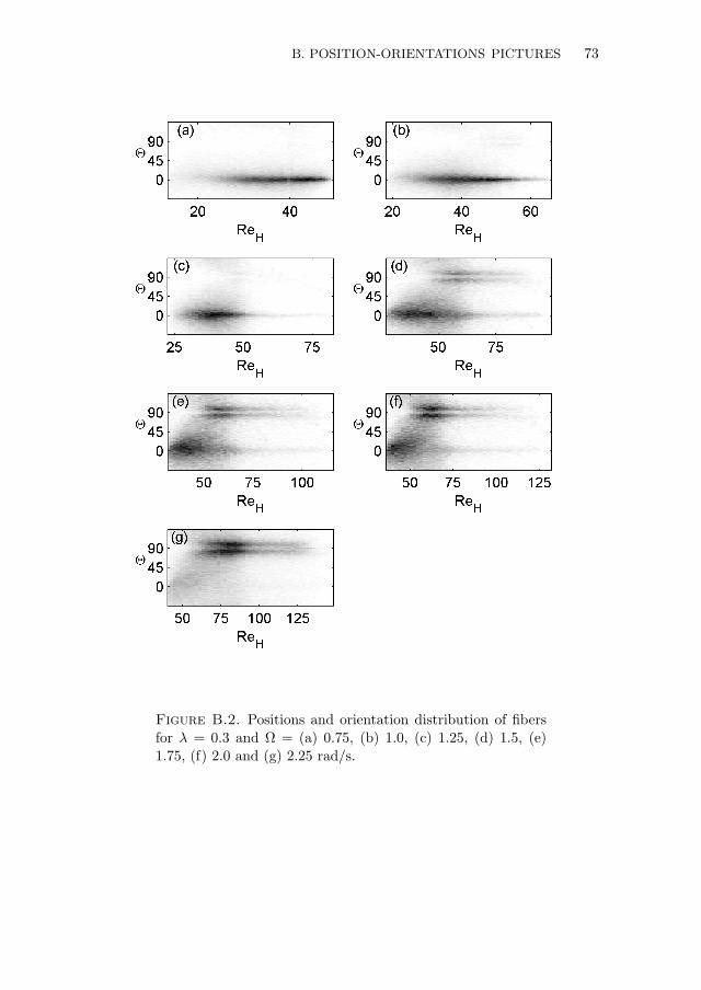
B. POSITION-ORIENTATIONS PICTURES 73
Figure B.2. Positions and orientation distribution of fibersfor λ = 0.3 and Ω = (a) 0.75, (b) 1.0, (c) 1.25, (d) 1.5, (e)1.75, (f) 2.0 and (g) 2.25 rad/s.

74 B. POSITION-ORIENTATIONS PICTURES
Figure B.3. Positions and orientation distribution of fibersfor λ = 0.4 and Ω = (a) 0.75, (b) 1.0, (c) 1.25, (d) 1.5, (e)1.75, (f) 2.0, (g) 2.25 and (h) 2.5 rad/s.
B. POSITION-ORIENTATIONS PICTURES 75
Figure B.4. Positions and orientation distributions of fibersfor λ = 0.5 and Ω = (a) 0.75, (b) 1.0, (c) 1.25, (d) 1.5, (e)1.75, (f) 2.0 and (g) 2.25 rad/s.
76 B. POSITION-ORIENTATIONS PICTURES
Figure B.5. Positions and orientation distributions of fibersfor λ = 0.6 and Ω = (a) 0.75, (b) 1.0, (c) 1.25, (d) 1.5, (e)1.75, (f) 2.0 and (g) 2.25 rad/s.

B. POSITION-ORIENTATIONS PICTURES 77
Figure B.6. Positions and orientation distributions of fibersfor λ = 0.7 and Ω = (a) 0.75, (b) 1.0, (c) 1.25, (d) 1.5, (e)1.75, (f) 2.0 and (g) 2.25 rad/s.
78 B. POSITION-ORIENTATIONS PICTURES
Figure B.7. Positions and orientation distributions of fibersfor λ = 0.8 and Ω = (a) 0.75, (b) 1.0, (c) 1.25, (d) 1.5, (e) 1.75and (f) 2.0 rad/s.

B. POSITION-ORIENTATIONS PICTURES 79
Figure B.8. Positions and orientation distribution of fibersfor λ = 0.9 and Ω = (a) 0.75, (b) 1.0, (c) 1.25, (d) 1.5, (e) 1.75and (f) 2.0 rad/s.