An Experimental Study into Spectral and Geometric Approaches to Data Clustering

Prashant Sridhar

October 2015

CMU-CS-15-149

School of Computer Science Carnegie Mellon University

Pittsburgh, PA 15289 Thesis Committee:

Dr. Gary Miller, Chair Dr. Alex Smola

Submitted in partial fulfillment of the requirements for the degree of Masters in Computer Science.

Copyright @ Prashant Sridhar

Keywords: Geometry, Nonparametric, Clustering

For my parents

AcknowledgmentsI would like to thank my advisor, Dr. Gary Miller, for allowing me to work with

him through this project.

vi

AbstractCommon clustering techniques involve assumptions on the distribution that the

data is drawn from, with linearity often being a standard assumption. These tech-niques work poorly on irregular data sets or on rare clusters. Non-parametric solu-tions are often inefficient to use in practice and still fail to find rare clusters. Thisthesis explores geometric approaches to non-parametric clustering that should bemuch better at identifying these rare clusters. The first approach explores how theGabriel graph can be used to compute density based distance metrics and how theGabriel graph itself might be used to cluster data. The second approach views theprobability density function as a heat distribution over a metal plate. Traditionally,finite element or control volume methods construct graphs over meshes on the metalplate. This approach explores how these meshes could be used to partition space.Finally, we present the results of running these clustering algorithms on flow cytom-etry data and compare these to present state of the art non-parametric methods onthe field.

viii

Contents

1 Introduction 1

2 Historical Spectral clustering 5

3 Density based distance metrics and clustering 93.1 Approximation of density based distance metrics . . . . . . . . . . . . . . . . . 93.2 Gabriel graphs and approximate Gabriel graphs . . . . . . . . . . . . . . . . . . 113.3 Weakly Gabriel graph and fast linear spanner . . . . . . . . . . . . . . . . . . . 163.4 Results and Discussion . . . . . . . . . . . . . . . . . . . . . . . . . . . . . . . 19

4 Geometric non-parametric clustering 254.1 Control volume methods . . . . . . . . . . . . . . . . . . . . . . . . . . . . . . 274.2 Constructing the mesh graph . . . . . . . . . . . . . . . . . . . . . . . . . . . . 28

5 Results 33

Bibliography 43

ix

x

List of Figures

3.1 Quadratic size Gabriel graph example . . . . . . . . . . . . . . . . . . . . . . . 133.2 Gabriel edges with small angle . . . . . . . . . . . . . . . . . . . . . . . . . . . 143.3 Candidate hyperplane elimination . . . . . . . . . . . . . . . . . . . . . . . . . 173.4 Barcode data clustered with a Gabriel graph . . . . . . . . . . . . . . . . . . . . 223.5 Barcode data clustered with a K-means . . . . . . . . . . . . . . . . . . . . . . . 23

4.1 3D slivers . . . . . . . . . . . . . . . . . . . . . . . . . . . . . . . . . . . . . . 284.2 Delauny triangulation of Barcode data with Steiner points added . . . . . . . . . 294.3 Voronoi diagram of Barcode data with Steiner points added . . . . . . . . . . . . 304.4 Kite between two points in three dimensions . . . . . . . . . . . . . . . . . . . . 31

5.1 Small data set . . . . . . . . . . . . . . . . . . . . . . . . . . . . . . . . . . . . 345.2 Barcode data set . . . . . . . . . . . . . . . . . . . . . . . . . . . . . . . . . . . 355.3 K-means on toy data set . . . . . . . . . . . . . . . . . . . . . . . . . . . . . . . 375.4 SamSPECTRAL on toy data set . . . . . . . . . . . . . . . . . . . . . . . . . . 385.5 Geometry based clustering on toy data set . . . . . . . . . . . . . . . . . . . . . 395.6 SamSPECTRAL on Barcode data . . . . . . . . . . . . . . . . . . . . . . . . . 405.7 Geometric approach on Barcode data . . . . . . . . . . . . . . . . . . . . . . . . 41

xi

xii

Chapter 1

Introduction

Clustering of data points is a problem that has existed in machine learning literature for quitesome time now. The general definition is to partition a data set into ”clusters” based on theirsimilarity. Clustering techniques have several applications to fields like computational biology,computer vision, robotics, and others. The defining characteristic of clustering that also makes itso powerful is that it is traditionally defined in the unsupervised sense. This means that data ispresented to the algorithms without any prior labels designating clusterings. This unsupervisednature is part of the appeal since unlabeled data is often easy to collect and quite plentiful, whilelabeling data is often laborious, requiring a human to hand label the data set. However, whileunsupervised learning is often easy to collect data for, it is notoriously difficult to judge whenthe algorithm has produced a good clustering.Parametric clustering methods often have a welldefined statistical interpretation, but perform poorly on data sets that do not satisfy the modelassumptions. Non-parametric methods, on the other hand, are either very slow to implementin practice or not very well defined statistically. This thesis provides a statistical basis for anon-parametric clustering method that is efficient in practice.

Spectral methods [21] are a popular way to cluster data sets non-parametrically. The datapoints are connected together to form a graph with heavy weight edges between similar pointsand light edges between dissimilar points. This graph can then be cut in order to generate theappropriate clustering. Strong edges will rarely be cut because they would greatly decrease thecut quality. Conversely, weak edges are encouraged to be cut in order to keep the cut valuelow. This leaves similar nodes in the same cluster while separating dissimilar nodes. As a non-parametric method, it is resistant to non-linearities in the data set, however, it is often quite slowto run in practice. If a complete graph of the data is constructed, storing the graph itself willrequire O(N2) space. While quadratic time algorithms are slow to run in practice on larger datasets, quadratic space algorithms are completely infeasible even on smaller samples. Storing thegraph itself will require several gigabytes of memory in data sets larger than a few ten thousandsof points preventing most computers from even loading the graph into RAM. Further, if the graphis to be partitioned into k clusters, algorithm will require finding the k largest eigenvalues ofgraph laplacian. If the graph is very near complete, and consequently the laplacian is very dense,this operation will be very expensive making it infeasible to run on anything but the smallestdata sets. Finally, deciding exactly how to weight the edges of the graph is still a matter of trialand error. The most common method is to use a Gaussian kernel to decide the edge weights, but

1

there is little statistical basis to this. It is merely a way to handle non-linearity of the input data.Choosing the bandwidth of this Gaussian kernel, again, must be done with grid search and crossvalidation.

The method of clustering proposed in this thesis solves all the problems mentioned above.Our method also relies on partitioning a graph, however, we provide some statistical explanationfor the edge weights. Additionally, our method constructs a graph with only a linear numberof edges in O(nlogn) time. This linear size graph is feasible to store and results in a sparselaplacian, which can also be solved easily. We view clustering of data points as a partitioning ofthe probability space. Our interpretation of a good partition is one separating two high densityregions while having a low cross-sectional cut volume. This encourages splitting up maximaacross lines drawn through density troughs. This idea is also very similar to sparsest cuts ongraphs and lends itself very easily to graphical interpretations. The goal is to construct a sparsegraph wherein cut quality is similar to that of the distribution generating the data. The probabilitydistribution can be viewed as a heat distribution over a metal plate. Such heat distributions canbe modelled by triangular meshes over the data with added Steiner points and can be solved bycontrol volume methods. Since the mesh is a triangulation, it will only have a linear number ofedges. The triangular mesh can then be cut with standard spectral methods in order to retrievethe clustering. More specifically, the mesh approximates second nearest neighbour distancesfor the distribution, but these distances can easily be used as an estimate of the density function.Since we are only concerned with clusters and not the point-wise estimation of density, we do notface the traditional problems faced by other knn approaches of having non-convergent variance[9]. Integrated over finite measure sets, variance of the estimator drops off with the size of thesample. Further, clusters of at least O(logn) elements should be identified by our approach sinceby Chernoff bounds, enough points will be sampled from these clusters to determine the cut.This gives provides a guarantee that small clusters will be identified by our approach. Finally,as a spectral, non-parametric method, this algorithm is insulated against non-linearities in thedata allowing it to identify clusters with non elliptical shapes. Thus, the approach overcomes theshortcomings of previous clustering algorithms.

This thesis serves mostly as an experimental exploration into the idea of sparse graphs fordata clustering since much of the theory is still being developed. Primarily, this paper focuseson data with ”rare” cluster populations and highly non-elliptical clusters that are difficult tocluster with standard methods like gaussian mixture modeling [7] or k-means. Specifically, wewill deal with flow cytometry data. Flow cytometry is a laser based approach to differentiatingbetween populations of cells based on certain bio markers on the cells surface or inside its body.Cytometers can take measurements from several thousands of cells per second leading to largedatasets. Flow cytometry is often used in the diagnosis of several health disorders includingvarious types of cancers. It is also used in clinical trials including research to autonomouslycompute prognoses for HIV patients. Many of these applications require clustering cell typesas a primitive before prediction can take place, and at present, such clustering is often done byhand. Several model based clustering algorithms have been developed for this problem such as,FLAME, flowClust, flowMerge. These methods are all mixture models over t-distributions orskew t-distributions. Skew t-distributions, in theory, should be able to account for eccentricitiesin the data, but the time complexity scales to the fourth power with dimension rendering it uselessin practice beyond 5 dimensions. Further, these model based methods often fail to find rare cell

2

populations which are of particular interest to biological applications. Non-parametric methodshave also been tried in this space and mostly rely on spectral clustering. SAMSpectral solves theissue of quadratic space by heuristically sampling data, which the authors call faithful sampling,to form a representative population. As with all heuristics, there is no theoretical basis to thisapproach and it provides no provable guarantees. Our geometric spectral clustering methodoutperforms SAMSpectral while being able to produce guarantees on quality and run time.

3

4

Chapter 2

Historical Spectral clustering

Given a set of data points x1, x2, . . . , xn and a notion of similarity sij , the goal of any clusteringalgorithm is to assign points of low similarity to different clusters while keeping high similaritypoints grouped together. Spectral clustering builds on the notions of graph cuts in order to achieveour goal of clustering. To do this, we build a similarity graph, G = (V,E). In this graph, eachvertex vi corresponds to a data point xi. Two vertices vi, vj are connected by an edge eij withweight equal to the similarity between the corresponding data points, sij . Clustering data pointscan now be rewritten to split the similarity graph into groups such that edges running betweendifferent clusters are weak while those running within a cluster are strong.

To begin with, we go over basic terminology and notation used in this chapter. Let G =(V,E) be the affinity graph defined on the data points with vertex set V = v1, v2, . . . , vn. G isan undirected graph with weighted edges such that the edge weight eij between vertices vi, vjis equal to then similarity function of the two data points sij ≥ 0. The degree di of vertex vi isdefined to be

di =∑j

eij

The graph has a corresponding weighting adjacency matrix A whose entries aij are definedas follows

aij =

0 if i = jsij otherwise

Finally, the degree matrix D of the graph, with entries dij , can be defined as follows

dij =

di if i = j0 otherwise

Consider a set of vertices A and its corresponding inverse set, V/A, the set of all vertices notin A. As shorthand, let A′ = V/A, and i ∈ A mean that vi ∈ A. Define the volume of A, |A| asfollows,

5

|A| =∑i∈A

eij

A serves as a partition of the vertices and there is a cut separating A from A′. Let cut(A,A′)be the surface area of the cut defined as follows,

cut(A,A′) =∑

i∈A,j∈A′eij

Therefore, |A| is the sum of edge weights such that both edge end points lie within A whilecut(A,A′) is the sum of edge weights such that only one end point is within A.

For data drawn from Rd, the similarity between two vertices can be defined in terms of theEuclidean distance between the corresponding points. We define sij = k(xi, xj) for some func-tion k based on only the distance between the two points. This function k must be monotonicallydecreasing on the distance to ensure that near by points are very similar while points far awayare very dissimilar. Traditionally, a Gaussian kernel is used for k.

k(xi, xj) = exp

(−||xi − xj||22

2σ2

)Where σ is a parameter(width) controlling the diameter of the clusters. Other methods of

constructing the similarity graph include only connecting each point to its k nearest neighbours,or only connecting it to points within an ε ball around it.

Given a similarity graph with an adjacency matrix A, and degree matrix D, define the graphlaplacian L as

L = D − A

The main tool of spectral clustering is the graph laplacian and its eigenvalues and eigenvec-tors. For example the number of connected components in a graph is equal to the number of 0eigenvalues in its graph laplacian. As discussed earlier, clustering on a graph can be phrased aspartitioning the vertex set so that the volume of each vertex cluster is large while the surface areaof the cut is small. This can be formalized in the Normalized cut. Let A1, A2, . . . Ak be the kpartitions of the vertices. Define NCut(A1, A,2, . . . Ak) as follows.

NCut(A1, . . . , Ak) =1

2

k∑i=1

cut(Ai, A′i)

|Ai|

Before detailing how to minimize the Normalized cut, define the normalized graph laplacianas follows

L = D−1L

The traditional spectral clustering algorithm proceeds as follows,

6

• Compute similarity graph G.• Compute normalized graph laplacian L.• Compute Λk, the matrix of the k smallest eigen vectors of L.• Run k-means on the columns of Λk.• Return the result as the cluster assignment for the data set.

It can be shown that this algorithm solves a relaxed version of the NCut problem. The prob-lem with spectral clustering is that results vary widely based on the type of similarity metricused and how points are connected to form a similarity graph. The rest of this thesis discussesprincipled approaches to solving this problem.

7

8

Chapter 3

Density based distance metrics andclustering

Our initial approach to combating the non-linearity of cytometry data, was to try non-euclideandistance metrics. Under a density based metric, two points are closer together if joined by apath through high density space, and farther apart if only connected through low density space.This should allow cluster detection even for clusters with highly non-elliptical shape. However,density based metrics are often intractable to compute exactly leading most such approaches touse reliable approximations. A recent approximation method developed by Choen et. al., [2],provides a graph based method to approximate a density based metric by computing shortestpaths on a Gabriel graph over the points. The final graph has a linear(in the points) number ofedges leading to quick single source shortest path queries. However, naive implementations ofk-means replacing Euclidean distance with density based distance will still run into the problemof having to store all pairs shortest paths. This will still require O(n2) space rendering theapproach infeasible. While, straightforward applications of the distance metric might not befeasible, spectrally cutting the Gabriel graph itself intuitively leads to a good clustering. Thissection of the thesis does not contain fully reasoned theory. Instead, it is an intuitive explorationof the usefulness of the Gabriel graph. While it is hard to arrive at provable bounds for clusterquality, Gabriel graphs are not as prone to the curse of dimension. While the number of edgesgrows exponentially with dimension, it is still upper bounded by O(n2), or the complete graph.On the other hand, the main method presented in this paper is based on Delauny triangulationsand require time exponential in the dimension to construct. Therefore, the Gabriel graph mayprovide a clue on how to deal with high dimensional data sets. Before explaining how to clusterusing the Gabriel graph, this thesis will first go over the work of Cohen et. al. to provide somebackground for the discussion and define relevant terms.

3.1 Approximation of density based distance metrics

If Rd space is Endowed with a distance metric, we can define the length of an arbitrary path γthrough this space as follows. Let the length function of a path under Euclidean distance be `e,and let γ begin at the point x at time 0 and end at the point y at time 1.

9

`e(γ) =

∫γ

ds

=

∫ 1

0

∣∣∣∣dγ(t)

dt

∣∣∣∣ dtWhich is simply the path integral of γ in Rd. Here,

∣∣∣dγ(t)dt

∣∣∣ is the velocity of trajectory at timet. Note that this integral is minimized by using the straight line path between the two points.Using this formulation for the length of a path, we can define the Euclidean distance, de betweenthe points x and y to be,

de(x, y) = infγ`e(γ)

This is merely a mathematical precise way of saying that the Euclidean distance between twopoints is the length of straight line shortest path between the points.

With Euclidean distance formally defined, this can now be extended to more general distancemetrics. By adding a cost function based on location in the space, segments of a path throughdifferent regions are priced differently thereby contorting the shortest path away from the straightline path between the points. Let the cost function for a certain metric k be c(x). We can nowdefine the length of a path γ for this metric, `k, as follows.

`k(γ) =

∫γ

c(s)ds

=

∫ 1

0

c(s)

∣∣∣∣dγ(t)

dt

∣∣∣∣ dtThere is also an analogous definition for distance, dk, for this metric.

dk(x, y) = infγ`k(γ)

Density based distance metrics penalize paths through low density regions and reward pathsthrough high density regions. Therefore, when used as a similarity metric, it will cluster togetherpoints belonging to the same high density regions. Let P be the probability distribution over Rd,and f(x) be its density function at point x. Define cp(x) = f(x)

2(1−p)d to be the cost function

used for the density based distance metric. Also define `p(γ) and (d)p(x, y) to be the associatedpath length function and distance metric. Note that p = 1 returns the Euclidean metric.

The problem with using density based metrics is that for p 6= 1, computing `p(γ) is near in-tractable for many distributions and paths. Often the true distribution is not even known and musttherefore be estimated. Worse, computing dp(x, y) involves finding an infimum over an infinitenumber of paths. Hence, the distance can never be exactly computed and must be approximated.

10

Assume that n points are uniformly randomly sampled from P to form the training data set D.We can now define an undirected graph G over these points such the edge length, exy;x, y ∈ D,is equal to the pth power of the Euclidean distance between the points, exy = de(x, y)p. DefinedG(x, y) to be the shortest path distance from x to y in the complete graph G. The followingtheorem from Hwang et. al., [12] proves a strong connection between dG(x, y) and dp(x, y) atthe price of a few assumptions on the sample space and the density function. Assume that P isinstead defined over a manifold M , the same manifold that D is drawn from.Theorem 3.1.1. Assume M is compact, and that f is continuous and supported everywhere overM . There exists a constant C(d, p) > 0, which only depends on d and p, satisfying the following.Let ε > 0 and b > 0, then there exists θ > 0 such that

P

(supx,y

∣∣∣∣∣ dG(x, y)

n(1−p)d dp(x, y)

− C(d, p)

∣∣∣∣∣ > ε

)< e−θn

1(d+2p)

for all sufficiently large n where x, y ∈M and de(x, y) ≥ b.In the case whereM is closed instead of compact, the paper presents a second theorem giving

an almost surely limit relating the two metrics.Theorem 3.1.2. Assume M is closed and that f is continuous and supported everywhere overM . There exists a constantC(d, p) > 0, which only depends on d, and p, satisfying the following.

limn→inf

np−1d dG(x, y) = C(d, p)dp(x, y)

for fixed x, y ∈M .The assumptions of note here are that M is either compact or closed. This means that the

theorems do not work in the general case where data can be drawn from anywhere in Rd. Inpractice, however, this assumption is not a problem because the set of valid data to be clusteredcan often be bounded between some finite intervals. The density function is also assumed to becontinuous and supported everywhere over its domain. This can be achieved by simply shrinkingits domain to only contain space in which f is supported. Since points cannot be drawn from0 probability regions, this assumption is easily met in practice. What these assumptions buythough, are strong bounds relating dp and dg thereby giving a way to approximate density baseddistance metrics. However, while computing shortest paths on G is tractable, computing G itselfrequires quadratic space rendering this approach useless on larger data sets. This problem can beavoided by considering the special case of p = 2, as is done by Cohen et. al.

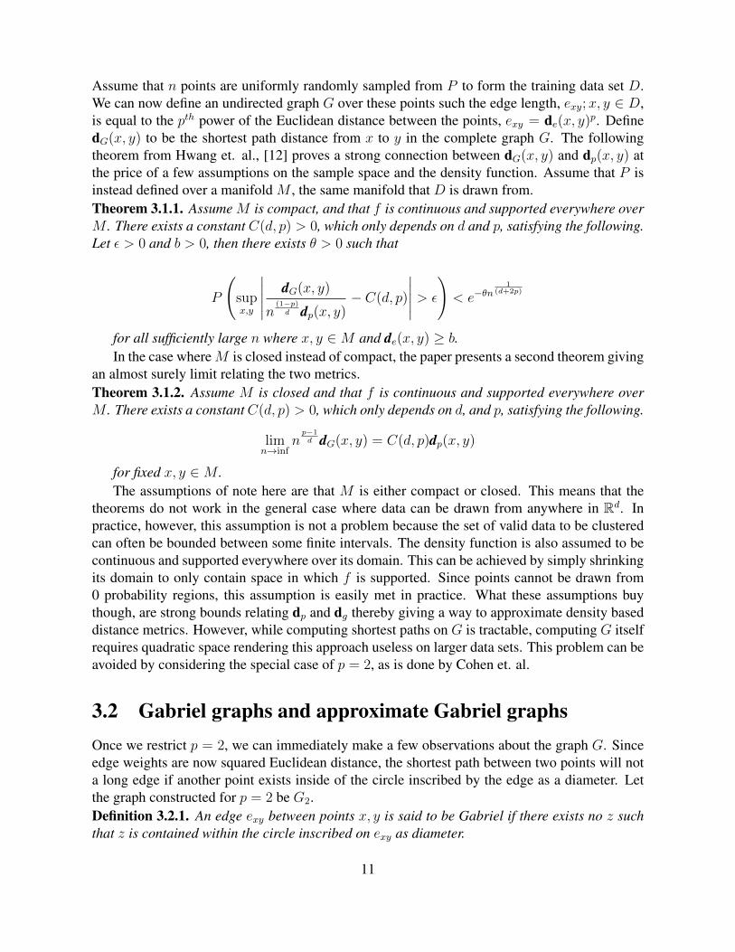
3.2 Gabriel graphs and approximate Gabriel graphsOnce we restrict p = 2, we can immediately make a few observations about the graph G. Sinceedge weights are now squared Euclidean distance, the shortest path between two points will nota long edge if another point exists inside of the circle inscribed by the edge as a diameter. Letthe graph constructed for p = 2 be G2.Definition 3.2.1. An edge exy between points x, y is said to be Gabriel if there exists no z suchthat z is contained within the circle inscribed on exy as diameter.

11

Lemma 3.2.1. For all x, y ∈ G2, the shortest path from x to y will only contain edges that areGabriel.

Proof. Assume for the sake of contradiction that the shortest path from x to y contains an edgeeuv that is not Gabriel. By 3.2.1, there exists a point z inside the circle formed using euv asdiameter. Consider the triangle formed by u, v, z. By the properties of triangles, the angle formedat z will be at least 90. Therefore, euv ≥ euz + evz by the Pythagorean theorem. Therefore wehave found a shorter path and have arrived at a contradiction.

Definition 3.2.2. The graph GG2, with V = D and E = ∪exy, exy is said to be the Gabrielgraph over the points in D.

Note that the set of Gabriel edges is a subset of Delauny edges since the Gabriel requirementis a stricter form of the Delauny requirement over edges.

The Gabriel graph serves as a possibly sparse graph that can be used to compute the densitymetric. Because the Gabriel graph is a subset of the Delauny triangulation, it serves as a linearspanner for d = 2. This is because the Delauny triangulation in the 2D case forms a planar graphwhich necessarily has a linear number of edges. However, even in 3 dimensions, examples can beconstructed where the Gabriel graph has O(n2) edges. Consider the unit sphere in 3 dimensionsand two small arcs on along this sphere on the XY plane and the Y Z plane with both arcscentered around Y = 0. Arrange n/2 points equally spaced on each arc. By construction,every edge between a pair of points on different arcs will be Gabriel since each of those edgesis approximately a diametric chord for the sphere. Therefore, this example leads to at least n2/4edges. This example can be seen in 3.1.

This prompts the need for spanners on the Gabriel graph. It is worth noting that even inhigher dimensional cases where the Gabriel graph is linear, there is no fast algorithm to computeit. The naive approach of checking if each edge is Gabriel requires O(n3) time even when onlya linear number of edges are Gabriel.

While very efficient algorithms [5], [3], working in O(nlogn), time exist for computingEuclidean spanners, these algorithms are still exponential in dimension because they rely onspace partitioning trees. In practice, these algorithms do not work well for d > 10. For thisreason, other approaches that do not scale so poorly with dimension are desirable.

While the original paper did not present a way to compute the Gabriel graph quickly, they dopresent an algorithm to produce a linear, (1 + ε) spanner given the Gabriel graph. The simpleconstruction involves constructing a conflict graph for each node p based on the angles formedby its neighbours. For any node p, construct a graph, Hp by connecting p to all its neighbours,and connect any pair of neighbours a, b if the angle formed by epa and epb is sufficiently small,say, smaller than θ. Define Ip to be the set of edges in the maximal independent set Hp. Thelinear spanner of the Gabriel graph is the graph Hθ such that

EHθ = (p, q)|epq ∈ (Ip ∪ Iq)

Before presenting the proof of quality for the spanner Hθ, we must first prove two supportinglemmas. We show that if two edges make a sufficiently small angle, then the length of the pathdoes not change by much depending on which we pick.

12

Figure 3.1: Quadratic size Gabriel graph example

13

Figure 3.2: Gabriel edges with small angle

Theorem 3.2.2. Consider a point p with neighbours q, r such that epq, epr are both Gabriel andmake an angle of at mot θ. Let A be the Euclidean length of epq and B be the Euclidean lengthof epr. Then it is the case that for any path through the graph containing epq, its length would notchange by more than (1 + 2tan2θ)|A|2 if epr were traversed instead.

Proof. Begin by noticing that we can assume eqr exists in the graph. If eqr is not in the graph,then it is not Gabriel, implying that there exists a point s within the circle with qr as diameter.Then, traversing eqs followed by esr would be shorter than directly traversing eqr. Therefore,eqr’s existence serves as an upper bound assumption for the stretch generated by not traversingepq and does not weaken the proof.

Let C be the Euclidean length of eqr. We want to show that |B|2 + |C|2 ≤ (1 + 2tan2θ)|A|2.

Without loss of generality, assume that p is at the origin, q is at (a, 0) and r is at (1, e). Thisis shown in 3.2

|C|2 + |B|2

|A|2=

(1− a)2 + e2 + 1 + e2

a2

=2− 2a+ a2 + 2e2

a2

This ratio is at its worst when a = 1, or when A and C are perpendicular. To see this,differentiate the above ratio with respect to a. The derivative is negative for 1 ≤ a ≤ 1 + e2. Fora outside of this range, either q or r will encroach on the ball of the other. Therefore, if the anglebetween A and B is less than θ,

14

|B|2 + |C|2

|A|2≤ |B|

2 + |B|2sin2θ

|B|2cos2θ

=1 + sin2θ

cos2θ= 1 + 2tan2θ

=⇒ |B|2 + |C|2 ≤ (1 + 2tan2θ)|A|2

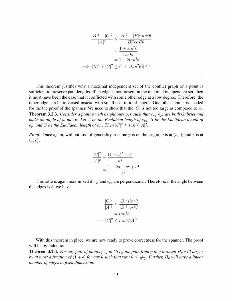
This theorem justifies why a maximal independent set of the conflict graph of a point issufficient to preserve path lengths. If an edge is not present in the maximal independent set, thenit must have been the case that it conflicted with some other edge at a low degree. Therefore, theother edge can be traversed instead with small cost to total length. One other lemma is neededfor the the proof of the spanner. We need to show that the |C| is not too large as compared to A.Theorem 3.2.3. Consider a point p with neighbours q, r such that epq, epr are both Gabriel andmake an angle of at mot θ. Let A be the Euclidean length of epq, B be the Euclidean length ofepr and C be the Euclidean length of eqr. Then |C|2 ≤ tan2θ|A|2.

Proof. Once again, without loss of generality, assume p is on the origin, q is at (a, 0) and r is at(1, e).

|C|2

|A|2=

(1− a)2 + e2

a2

=1− 2a+ a2 + e2

a2

This ratio is again maximized if eqr and epq are perpendicular. Therefore, if the angle betweenthe edges is θ, we have

|C|2

|A|2≤ |B|

2sin2θ

|B|2cos2θ= tan2θ

=⇒ |C|2 ≤ tan2θ|A|2

With this theorem in place, we are now ready to prove correctness for the spanner. The proofwill be by induction.Theorem 3.2.4. For any pair of points p, q in GG2, the path from p to q through Hθ will largerby at most a fraction of (1 + ε) for any θ such that tan2 θ ≤ ε

2+ε. Further, Hθ will have a linear

number of edges in fixed dimension.

15

Proof. This theorem will be proved using induction over the length of the longest edge in a path.For the base case, consider (p, q) the closest pair in the data set. Since they are the closest pair,p is q’s nearest neighbour. Nearest neighbour edges are always Gabriel because if they were not,a point would lie within the circumscribing circle thereby generating a nearer neighbour. epq isalso in Hθ because if it were not, then it must conflict with another edge, say, epr. By 3.2.3, eqrmust be shorter still meaning p, q is not the closest pair.

For the inductive step, assume that for all paths between pairs (p, q) with longest edges shorterthan |A|, Hθ is a (1 + ε) spanner. Now consider all path with a longest edge of length |A|. If thisedge is in Hθ, then the above theorem holds. If the edge is not in Hθ, then it must conflict withsome neighbour. Let the endpoints of the longest edge be p, q, and the end points of the edge itconflicts with be p, r. Let B be the length of epr be |B| and the length of eqr be |C|. Let P bethe path from q to r in Hθ. Since |C|2 ≤ tan2θ|A|2, the shortest path from q to r in GG2 cannothave any edges as long as |A|. Therefore by the inductive hypothesis,

|P | ≤ (1 + ε)|C|2

Again, note that if eqr is not in GG2, the length of the path would be even shorter. Hence theassumption that eqr is in GG2 is an overestimate.

We now want to bound |B|2 + |P | since that is the path from p to q in Hθ.

|B|2 + |P | ≤ |B|2 + |C|2 + ε|C|2

≤ (1 + 2tan2θ)|A|2 + εtan2θ|A|2

≤ (1 + (2 + ε)tan2θ)|A|2

≤ (1 + ε)|A|2

Finally, Hθ must have a linear number of edges in a fixed dimension because in any fixeddimension, each node may only have a constant out degree when constrained to only have neigh-bours separated by a minimum degree.

3.3 Weakly Gabriel graph and fast linear spanner

The last section went over how to construct Gabriel graphs to compute density based distancemetrics and how to sparsify these graphs. This section weakens the conditions on Gabriel graphsto allow for faster algorithms to construct them. Further, we show that we can sparsify these moregeneral Gabriel graphs to still retain linear sized graphs. To begin with, we define the notion ofan edge being weakly Gabriel. The edge to a neighbour is said to be weakly Gabriel if there areno other neighbours within the dihedral ball of the edge. However, other, non-neighbours arestill allowed to encroach the ball. Formally, we define weakly Gabriel as follows,

16

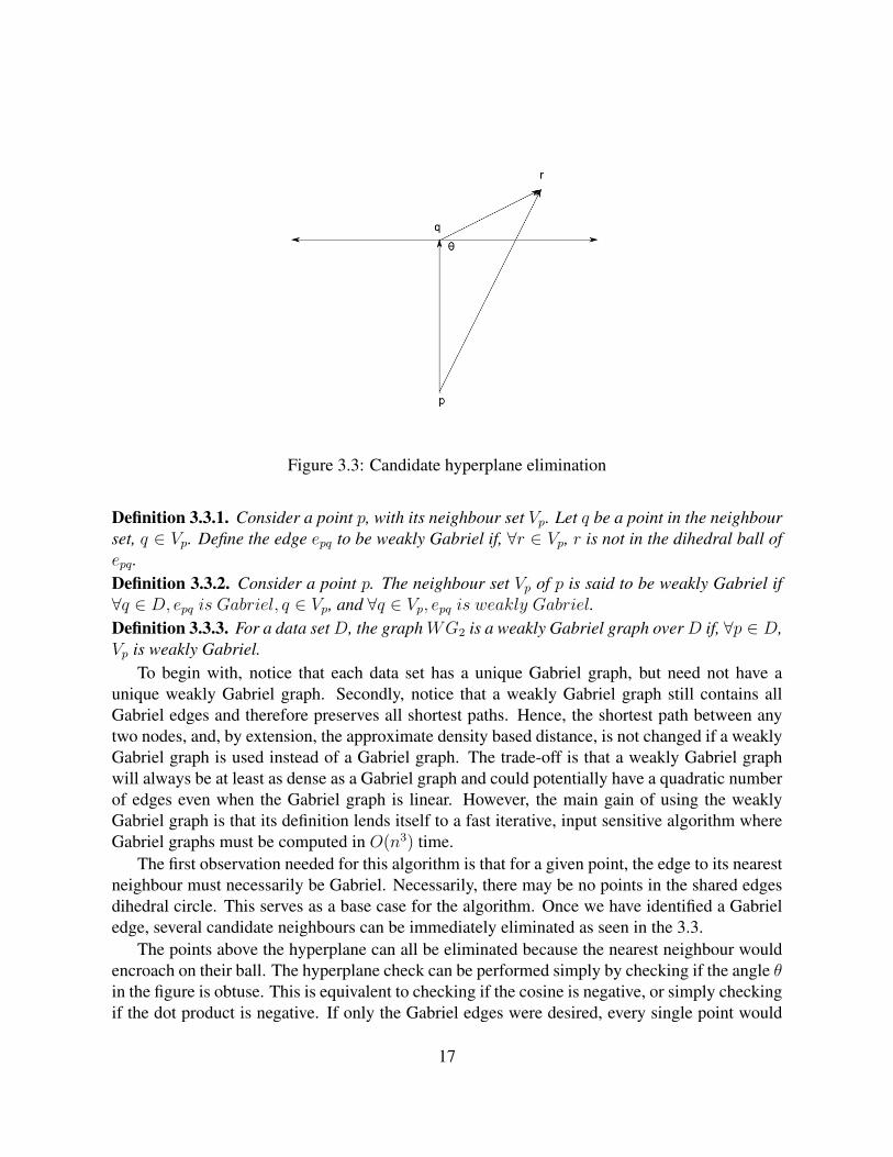
Figure 3.3: Candidate hyperplane elimination

Definition 3.3.1. Consider a point p, with its neighbour set Vp. Let q be a point in the neighbourset, q ∈ Vp. Define the edge epq to be weakly Gabriel if, ∀r ∈ Vp, r is not in the dihedral ball ofepq.Definition 3.3.2. Consider a point p. The neighbour set Vp of p is said to be weakly Gabriel if∀q ∈ D, epq is Gabriel, q ∈ Vp, and ∀q ∈ Vp, epq is weakly Gabriel.Definition 3.3.3. For a data setD, the graphWG2 is a weakly Gabriel graph overD if, ∀p ∈ D,Vp is weakly Gabriel.

To begin with, notice that each data set has a unique Gabriel graph, but need not have aunique weakly Gabriel graph. Secondly, notice that a weakly Gabriel graph still contains allGabriel edges and therefore preserves all shortest paths. Hence, the shortest path between anytwo nodes, and, by extension, the approximate density based distance, is not changed if a weaklyGabriel graph is used instead of a Gabriel graph. The trade-off is that a weakly Gabriel graphwill always be at least as dense as a Gabriel graph and could potentially have a quadratic numberof edges even when the Gabriel graph is linear. However, the main gain of using the weaklyGabriel graph is that its definition lends itself to a fast iterative, input sensitive algorithm whereGabriel graphs must be computed in O(n3) time.

The first observation needed for this algorithm is that for a given point, the edge to its nearestneighbour must necessarily be Gabriel. Necessarily, there may be no points in the shared edgesdihedral circle. This serves as a base case for the algorithm. Once we have identified a Gabrieledge, several candidate neighbours can be immediately eliminated as seen in the 3.3.

The points above the hyperplane can all be eliminated because the nearest neighbour wouldencroach on their ball. The hyperplane check can be performed simply by checking if the angle θin the figure is obtuse. This is equivalent to checking if the cosine is negative, or simply checkingif the dot product is negative. If only the Gabriel edges were desired, every single point would

17

have to draw its hyperplane and eliminate potentially offending points. However, this will againrequire O(n3) time. Instead, we need only eliminate points with successive nearest neighboursin order to obtain a weakly Gabriel neighbour set. This is formalized in 1

Algorithm 1: Compute Weakly Gabriel GraphData: Data set DResult: Weakly Gabriel Graph, WGG = V, Vp over DWGG←− for p ∈ D do

Vp ←− for p ∈ D do

dp ←− [ ]for q ∈ D − p do

append(dp, (q,d2e(p, q))

sp ←− sort(dp) ascending by distancewhile sp is not empty do

r ←− pop(sp) for s ∈ sp doif cos(rp, rs) > 0 then

remove(sp, s)

add(Vp, r)

add(WGG, p, Vp)for q ∈ Vp do

if p /∈ Vq thenadd(Vq, p)

The run time of this algorithm is O(n2logn) for the sorting step, and O(n2e) for the elimina-tion steps, where e is the maximum out degree of a point. In practice, this algorithm works wellat building a sparse graph on which to run shortest path queries because many real world datasets have linear size Gabriel graphs. For those applications, The weakened Gabriel graph algo-rithm produces only a small fraction of non-Gabriel edges. For example, in one flow cytometrydata-set consisting of roughly 70,000 points in 16 dimensions, only 2% of the edges generatedwere non-Gabriel. This highlights the algorithms input sensitivity. In most practical use cases,the bottle-neck in runtime is the sorting step giving an overall complexity of O(n2logn) sincee is often a constant. However, it is possible to construct edge cases with a linear number ofGabriel edges for which 1 produces a quadratic number of edges leading to a O(n3) time andO(n2) space complexity.

The good news is that sparsifying based on angle will continue to work on weakly Gabrielgraphs. If a non-Gabriel edge is ever picked in favour of a Gabriel edge, the stretch will stillremain small because the edges must be comparable in length. If this were not the case, onewould encroach on the dihedral ball of the other violating the requirement that both edges be atleast weakly Gabriel. This preserves lemmas, 3.2.2 and 3.2.3. With these lemmas in place, themain proof carries through very similarly.

18

Instead of first running 1 and then sparsifying the resultant graph, the two steps can be com-bined into one. When a point is added to the neighbour set and used to prune potential neigh-bours, the only check performed is the hyperplane check. Instead, the neighbour can prune pointsby its hyperplane and also by the angle made with p. Finally, because the resultant graph willhave constant(in dimension) out degree from each node by virtue of being a linear spanner, thesorting step can be removed in favour of picking the closest neighbour each time. Since we willonly have to pick a linear number of neighbours, this reduces the runtime from O(n2logn+n2e)to O(n2e), which is the same as O(n2). This algorithm is formally represented in 2

Algorithm 2: Compute Sparse Weakly Gabriel GraphData: Data set DData: Error threshold εResult: Weakly Gabriel Graph, WGG = V, Vp over DWGG←− for p ∈ D do

Vp ←− for p ∈ D do

dp ←− [ ]for q ∈ D − p do

append(dp, (q,d2e(p, q))

while dp is not empty dor ←− findmin(dp)remove(dp, r)for s ∈ dp do

if cos(rp, rs) > 0 || tan2(pr, ps) > ε2+ε

thenremove(sp, s)

add(Vp, r)

add(WGG, p, Vp)for q ∈ Vp do

if p /∈ Vq thenadd(Vq, p)

3.4 Results and Discussion

While asymptotically we can achieve O(n2), in practice it is often faster to perform the sortingstep and run atO(n2logn). It can be shown that for a point placed on the origin and surrounded byneighbours drawn uniformly from the unit ball, the expected number of Gabriel edges is O(2d).It can also be empirically observed that the average angle between edges is 90. Therefore, eachnode often has a large out degree making repeatedly picking the nearest neighbour very slow if2d exceeds logn. This also demonstrates that for data with no irregularities, sparsification is notnecessary and constructing a weakly Gabriel graph is sufficient. Also, the number of non-Gabriel

19

edges added by 2 is a very small percentage of the total edges. For the applications discussed inthis paper, no more than 5% of the edges generated are non-Gabriel. Therefore, 2 is a significantimprovement in computing approximations to density based distance.

Clustering with non-Euclidean distance metrics poses a challenge because computing themean of a cluster is difficult thereby rendering k-means impossible to use. The solution is toassume that the cluster center will be a point in the data set. This gives rise to the k-medioidsalgorithm [13]. The most common realization of the idea is Partitioning Around Mediods (PAM)[22] which proceeds as follows.

• Select k random points without repetition to serve as cluster medioids.• Assign each point to a cluster based on medioid distance.• Compute total cost of clustering and repeat until cost converges

For each medioid m and non-medioid o

− Swap m and o and recompute cost.

− Keep swap if cost decreases.

Other medioid based algorithms also exist such as the following based on Voronoi iterations[16].

• Select k random points without repetition to serve as cluster medioids.• Assign each point to a cluster based on medioid distance.• Compute total cost of clustering and repeat until cost converges

For each cluster, select m as medioid if m minimizes the sum of distance to all otherpoints.

Reassign points to the closest medioid.

If the number of iterations required to converge is assumed to be t and that pairwise distancesare stored in a Gram Matrix G, then the runtime of PAM is O(tkn2). Each internal step re-quire O(n2) time to swap a medioid with each non-medioid point and recompute the cost. Thesecond method also has a similar runtime of O(tkn2) since it take O(n2) time to find the opti-mal medioid for each cluster. The advantage of the second approach is it more closely mirrorsthe more familiar k-means algorithm and is this easier to reason about. The main drawback toboth of these approaches is that when the distance metric is density based distance, computingthe distance between two points requires a shortest path computation using Dijkstra’s algorithm,which will cost O(enlogn) where e is the maximum out degree. This makes computing distanceon the fly infeasible. The other alternative is to precompute all pairs shortest paths and store theresult in a Gram matrix. However, computing and storing the Gram matrix will have a O(n2)space complexity. While this approach is not further explored in this thesis, a solution to thisproblem might arise from the graph structure used to compute density based metrics. To begin,let us define the notion of closeness centrality [19] in a graph. The closeness centrality C(x) of agraph is defined as follows, C(x) = 1∑

y de(y,x)2 . The reciprocal of the closeness centrality is thedistance from a node to all the other nodes in the graph. This is very similar to the k-medioidsrequirement of computing the distance from the medioid to every other node in the cluster. Sev-eral algorithms such as [23][17][6] deal with computing closeness centrality or a related metric

20

called betweenness centrality [8] which is often considered harder to compute than closenesscentrality. These algorithms rely on sampling to build approximations to closeness and the meth-ods therein could significantly speed up medioid computation. Sampling techniques could alsobe useful in cluster assignment since the subsampled paths or nodes could build approximationsto the distance to different medioids for each point.

The other alternative is to cluster directly based on the properties of the Gabriel graph. Insteadof setting the edge weight exy to be the squared Euclidean distance, exy = de(x, y)2, set the edgeweight to be the reciprocal, exy = 1

de(x,y)2 . Geometrically close points in this graph are usuallyconnected by a single Gabriel edge or a series of short hops. In either of those cases, short edgeswill have very high weights leading the cut between the points to be very expensive. On the flipside, long edges on the graph are not very common since they are very likely to have some otherpoint encroach on them. They mostly arise from the boundaries of clusters. These long edges arealso much cheaper to cut than short edges, thereby incentivising cuts between clusters. In non-sparsified Gabriel graphs, there is some chance that there many connecting edges between twoclusters if the clusters are sufficiently compact and far away. This is similar to the scenario whereO(n2) Gabriel edges exist in the graph. These dense inter cluster connections are problematic forclustering because they drive up the cost of cutting the two clusters with several nearly identicaledges. Sparsified Gabriel graphs fix this issue by removing such ”duplicate” edges. If severaledges arise from and end with similar nodes, the edges will make small angles with each otherand will hence be pruned. This makes sparsified Gabriel graphs very good to cluster over. Notethat instead of the reciprocal of the squared Euclidean distance, a gaussian kernel could havebeen used for edge length. While results vary, they do not change significantly by altering thekernel. The weights that are mentioned in this section are used because they tie in to ideas ofeffective resistance and conductance of the edges. The experimental results section will go intomore detail but for now consider figure 3.4 of a clustering constructed by partitioning Gabrielgraphs.

The data set used here is called the Barcode data [11] set and it captures the difficulty ofclustering rare populations. The Barcode data set also provides an easily verified correct answerthat is not available for other flow cytometry applications(where experts often also disagree onclusterings). If we contrast the quality of this clustering with K-means, we see that cutting theGabriel graph performs much better. The primary win of this approach is that the Gabriel graphis still fast to construct in high dimensions. While the runtime will depend on the dimensionalityof the data, the number of edges in the graph is bounded by O(n2) and since 2 is an input sen-sitive algorithm, the runtime of that algorithm is also bounded. On the other hand, the approachmentioned later in this thesis requires computing the Delauny triangulation, a procedure thatscales exponentially with dimension. The primary downside of Gabriel graphs is that clusteringon them is not based soundly in theory while this is not true for the approach to be discussedin the next chapter. However, our algorithm grounded in theory still calls upon the Delauny tri-angulation, and since Gabriel edges are a subset of the Delauny edges, the Gabriel graph mightserve as an approximation to the more principled clustering approach in high dimension.

21

Figure 3.4: Barcode data clustered with a Gabriel graph

22

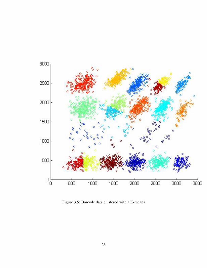
Figure 3.5: Barcode data clustered with a K-means

23

24

Chapter 4

Geometric non-parametric clustering

In this section we present a statistical framework to clustering and a geometric approach to solvethe resulting optimization problem. The goal of this section is to quickly compute linear graphswith which to cluster. Further, we ground the graphs built in theory in order to prove bounds onthe quality of the clusters obtained.Traditionally, spectral clustering does not have a statisticalinterpretation behind it. However, spectral clustering relies on notions of graph cuts. Define theNormalized cut (NCut) [21] as follows,

NCut(A1, . . . , Ak) =1

2

k∑i=1

cut(Ai, A′i)

|Ai|

Here, A1, . . . , Ak are the k partitions of the node set of the graph. |Ai| is the volume of acluster and is equal to

∑j,k ejk such that xj or xk ∈ Ai. A′i is the set of nodes in the graph that do

not belong to Ai. Finally, cut(Ai, A′i) is the surface area of the cut separating Ai from the rest ofthe graph. cut(Ai, A′i) =

∑j,k ejk such that xj ∈ Ai, xk ∈ A′i. Note that the quantity is divided

by 2 so as to not double count the edges.The most common definition of graph cuts is defined as follows,

cut(A1, . . . , Ak) =1

2

∑i

cut(Ai, A′i)

However this definition does not provide good clusters because there is strong incentive toremove single nodes with small out degree. The normalized cut circumvents this problem bynormalizing by cluster volume thereby encouraging larger clusters. The NCut quality would beminimized by ensuring that |Ai is the same for all i, i.e. equal volume clusters. As explainedin the section on spectral clustering, the spectral clustering algorithm solves a relaxed version ofthe normalized cut problem.

In this thesis, we extend the notion of normalized cuts to probability distributions. Define theNormalized Distribution cut (NDCut) as follows,

25

NDCut(A1, . . . , Ak) =1

2

k∑i=1

∮γ(Ai.A′i)

dA∫AidV

At this point it is important to note the k-way expansion cut [14]. Let the cut, Kcut, be definedas follows.

Kcut = max

(cut(Ai, A

′i)

|Ai|, i = 1, . . . , k

)This k-way expansion cut more closely resembles the isoparametric cut for which Cheeger

bounds exist [1]. Cheeger bounds bound the quality of this cut by the second eigenvalue of thegraph laplacian. Unfortunately, similar bounds do not exist for the normalized cut. While the k-way expansion cut has good theoretic properties, practitioners still use normalized cuts for theirlink to spectral clustering. In this thesis, we will continue to do the same.

In this context, letAi be a closed subspace of Ω corresponding to a cluster. A′i is the conjugatespace of Ai, A′i = Ω − Ai.

∫AidV is the volume integral of Ai and γ(Ai, A

′i) is the surface

seperating Ai from A′i. This means∮γ(Ai,A′i)

dA is the surface integral of the cut seperatingout Ai. The intuition behind the normalized distribution cut is very similar to that of the vanillanormalized cut. The formulation encourages cutting the probability space into maximum volumeclusters such that the surface area separating them is minimized. Since this formulation makesno assumptions on the underlying distribution, it remains non-parametric. Further, in order toprove effectiveness on small clusters, it only needs to be shown that volume and surface areaestimates are close even if only a few points from the cluster are sampled. As we do not haveaccess to the true density distribution, the density function must be approximated from the data.For this purpose, we will use a second nearest neighbour approximator.

Density approximation is traditionally done in two forms, k nearest neighbours and kernelmethods. Both methods involve measuring the number of points in a region as an approximationof density. KNN typically constrains the number of points in the region to be fixed (k) and adjuststhe radius until a large enough volume in covered. Conversely, kernel methods hold the regionvolume constant while counting the number of points in the space. For the purposes of the paper,we will use a second nearest neighbour estimator. For both approaches, say we are interested ina density approximation of points X , f(X). Let L(X) be a small neighbourhood of X . If L(X)is sufficiently small, the probability mass of L(X) can be approximated by f(X)v where v isthe volume of the local neighbourhood. The probability mass of the empirical region can alsobe approximated by sampling a large number of points from the distribution and counting thenumber that fall within L(X). Let n points be sampled and let k of them fall within L(X). Letf(X) be the desired empirical estimate of density at X .

f(X)v =k

N

f(X) =k

Nv

26

As was mentioned, KNN estimators work by varying v until k points fall in the local neigh-bourhood of X . However, the form of the estimator must be slightly modified as follows. Let vrbe the distance of the kth nearest neighbour to X . Let vr be the volume of the d dimensional ballof radius r. Again, let f(X) be the empirical density estimate.

f(X) =k − 1

Nvr

As shown in [10], the reason k − 1 is used instead of k in the numerator is that the formerleads to an unbiased estimator. With this modified form, it can be shown that the bias of the KNNestimator goes to 0 as n goes to infinity. However, the variance of the estimator remains constantas n increases and only reduces by increasing k. If accurate pointwise estimates are required,it can be shown that k must be some function of n. Our needs do not face this shortcomingbecause we are not interested in accurate pointwise estimates; rather, we are interested in accurateintegrals of the pdf over volumes of clusters or surface areas of cuts. While the proofs have not yetbeen completed rigourously, we believe that the large variance will integrate out as we considerlarger spaces. For any clusters of non-zero measure, it should be possible to invoke Chernoffbounds and claim that if it had a sufficiently large probability mass, sufficient points must fall inthe area to generate an accurate estimate.

4.1 Control volume methodsWith a pointwise estimate of density in place, we are ready to construct a graph to partition inorder to derive our clusters. For this purpose, a probability density distribution can be thoughtof as analogous to a heat distribution over a metal plate of varying conductivity. Regions ofhigh density can be thought of as parts of the metal plate with high conductivity. Solving theheat equation over a space is hard to do exactly but can be approximated well by finite elementmethods. Finite element methods solve partial differential equations over closed sets by splittingthe set into small units and solving the equation on unit boundaries. The total solution can thenbe extracted from these boundary solutions. In the 2D case, space is usually quantized by atriangulation.

In order to ensure an accurate approximation, it is important that the triangles be close toequilateral in some sense. This condition is achieved by bounding the aspect ratio for each tri-angle in the mesh. The aspect ratio of a triangle is defined to be the ratio of the radius of thecircumcircle to the smallest edge in the triangle. Ruppert’s algorithm [18] provides a mesh com-posed entirely of these high quality triangles. The algorithm consits of the following operationsand invokes the Delauny Triangulation [4] as a subroutine.

1. Compute the Delauny Triangulation of the points.

2. Repeat the following two steps until convergence.

3. For each segment such that its dihedral ball is non-empty, add its midpoint to the triangu-lation.

4. For each triangle with bad aspect ratio, add its circumcenter to the triangulation.

27

Figure 4.1: 3D slivers

In 3D, the mesh is generated by covering space with tetrahedrons. This, however, is plaguedby ”sliver” tetrahedrons in which the four points are nearly coplanar. Finite element methodsperform poorly in meshes containing these slivers despite their having good aspect ratio. Animage of these slivers can be found in, [15]. The image is reproduced here in 4.1. [15] showsthat the control volume method has a low error even in the presence of these slivers. There-fore, extensions of Ruppert’s algorithm can be used to solve estimation problems even in threedimensions.

4.2 Constructing the mesh graph

The problem remains to construct a graph over the input data as opposed to simply over a bound-ing box. In order for the control volume method to be applicable, it is still necessary for theVoronoi cells in the mesh to have good aspect ratio. In lower dimensions, this implies good as-pect ratio Delauny triangles. This is ensured by adding extra points to the data set called Steinerpoints. The Steiner points added can be shown to have the following properties.Theorem 4.2.1. For any data set D with n points, Steiner points D′ added to ensure the trian-gulation only has good aspect ratio triangles will increase the size of the data set by at most aconstant fraction.Theorem 4.2.2. For any data set D with n points, Steiner points D′ added to ensure the tri-angulation only has good aspect ratio triangles will not increase the second nearest neighbour

28

Figure 4.2: Delauny triangulation of Barcode data with Steiner points added

29

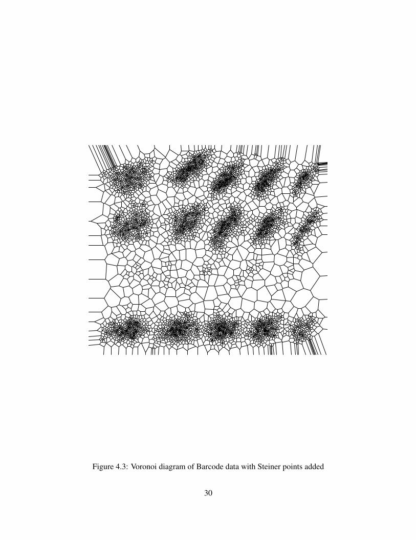
Figure 4.3: Voronoi diagram of Barcode data with Steiner points added

30

Figure 4.4: Kite between two points in three dimensions

distance of any point by at most a constant fraction.

Theorem 4.2.3. For any data set D, consider any point x. Let Steiner points D′ be added toenforce quality of the triangulation. Then the edge length from x to any of its neighbours will notdiffer by more than constant fraction.

These theorems allow us to triangulate the data set and ensure that all triangles have goodquality. The resulting triangulation graph is used as the affinity graph in order to cluster the dataset. In order to estimate the cut, boundary conditions on this graph must be solved. Considerthe figure 4.4 from [15]. This figure represents the connection between two neighbouring pointsin the triangulation, also known as a kite. The points are, without loss of generality, positionedalong the z-axis.Let the points be xi and xj and the Delauny edge between then be hij . K+ andK− refer to sections of the Voronoi space of each point. Aij is the Voronoi face between thetwo points. Let eij denote the weight of the edge in the affinity graph and h and A denote thelength of the edge and surface area of the Voronoi face respectively. Let Cij be the conductanceat the mean of the Voronoi face. The Control volume method dictates that the edge weight of theDelauny edge is as follows.

31

eij =A

hCij

=A

h

k − 1

nvh

= CA

h(d+1)

For some constant C. This is because the conductance on the Voronoi face is simply thedensity estimate at that point. This estimate is equal to k−1

nvh. Note here that k = 2 since we use

second nearest neighbour distance. In d dimensional space, vh = C ′hd for some other constantC ′. Combining these observations and separating the constants into a single term gives us theabove form. Because this constant is independent of position and therefore edge independent, itmay simply be dropped in assigning edge weights.

32

Chapter 5

Results

In this paper, we apply our clustering approaches to flow cytometry data. Cytometry refers tothe measurement of cell characteristics such as size, count, DNA content, or the existence ofcertain bio markers. Flow cytometry in particular refers to the measurement of cell characteris-tics by aligning cells using flow techniques. Cytometry data provides valuable insight into cellpopulations and is used often in medical research and diagnostics. Its applications include pro-viding diagnosis and prognosis information on diseases like HIV or leukemia. Clustering thesecell populations is a standard first step in many pipelines using cytometry data. However, thesedata clusters tend to be highly irregular in shape. Further, rare cell populations are often vitalto perform diagnostics. Therefore, traditional clustering methods such as K-means or GaussianMixture Models fail to produce satisfactory results.

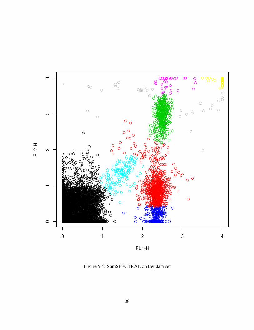
The state of the art non-parametric clustering approach on this data is SamSPECTRAL [24].SamSPECTRAL is also based around spectral clustering but constructs a complete graph overthe data. Rather than attempt to reduce the size of the graph, the algorithm relies on a heuristicto sample a ”representative” subset of the data points. The graph is then built only over theserepresentatives. The edge weight between points in the graph depend on the pairwise distancebetween all points assigned to each representative. This graph is then cut in order to cluster thedata set. Finally, clusters with low separation are combined. While SamSPECTRAL performswell on cytometry tasks, it relies heavily on heuristics and provides no theoretical bounds onquality.

Flow cytometry data poses another challenge and that is that the output of a clustering al-gorithm is hard to judge. Typically, cytometry data is somewhat high dimensional. Standardcytometry data sets contain 70,000-150,000 cells per person with 16-20 different measurementsper cell. Therefore, clusters must be judges in 20 dimensions. Even if dimensionality reductiontechniques are used, the problem is sufficiently hard that expert judgements are required. Cy-tometry data is nuanced enough that non-experts cannot easily determine the number of clustersor the cluster positions while expert annotated data sets are hard to come by. For this reason,much of the research is done on ”toy” data sets to demonstrate feasibility of the approach. Wepresent our approaches on two toy data sets. The first is a small set of non-linear data with afew rare populations. The second is a so called ”Barcode” data set that was presented in Section3.4. The data is reproduced here without clustering labels. This data has been built by experts toresemble problems faced in clustering true cytometry data and is presented here [11]. However,

33

0 1 2 3 4

01

23

4

FL1-H

FL2-H

Figure 5.1: Small data set

34

Figure 5.2: Barcode data set

35

the barcode data is easy for a non-expert to cluster on inspection.In the small toy example, both SamSPECTRAL and our clustering approaches vastly outper-

form K-means. Geometric clustering performs about as well as SamSPECTRAL (depending onthe designation of clusters) but is far less dependent on external parameters being set to the rightvalues. In order for SamSPECTRAL to perform well, several parameters must be tuned throughan exhaustive grid search.

The following pages contain the different clusterings for the toy data set and the barcodedata set. 5.3 is the figure showing the results of K-means on the toy data set. 5.4 presents howSamSPECTRAL clusters the set, while 5.5 shows the clustering produced through a geometrybased approach.

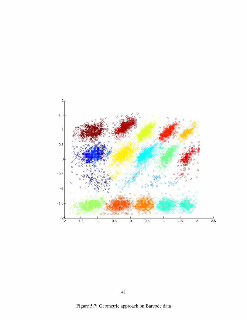
Similarly, ?? is the result of applying K-means to the Barcode data, 5.6 is the clustering pro-duced by SamSPECTRAL and 5.7 is the clustering produced by the geometry based approach.Finally, ??

For the Barcode data, we immediately notice that all approaches make mistakes. K-meansperforms the worst with several split clusters. SamSPECTRAL provides clear clusters but cannotdifferentiate between the several rare groups. It only detects the presence of 16 clusters instead of20. Both Gabriel clustering and Geometric clustering give similar results. Geometric clusteringhas a huge win on speed in low dimensions because computing a good quality triangulation isvery fast while computing the Gabriel graph is still super-quadratic time. Triangulation is donewith the help of the Triangle package. [20].

These results show that, in 2D, a geometry based approach is both very fast and decentlyperformant at identifying rare clusters. Spectrally clustering a mesh with Steiner points addedperforms similarly to SamSPECTRAL, a highly tuned, heuristic method. Further, meshing datasets in low dimensions is computationally cheap and produces only a linear sized graph. Inhigher dimensional problems, Gabriel graphs are cheaper to construct while still yielding goodclustering results and a linear graph. Further, the geometric approach has a strong theoreticalfoundation from which proofs of quality could be derived. This is a good avenue for futureexploration.

36

0 1 2 3 4

01

23

4

FL1-H

FL2-H

Figure 5.3: K-means on toy data set

37

0 1 2 3 4

01

23

4

FL1-H

FL2-H

Figure 5.4: SamSPECTRAL on toy data set

38

−1.5 −1 −0.5 0 0.5 1 1.5 2 2.5 3 3.5−1.5

−1

−0.5

0

0.5

1

1.5

2

2.5

3

3.5

Figure 5.5: Geometry based clustering on toy data set

39

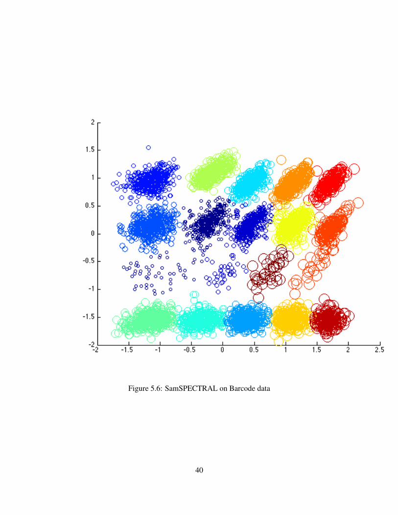
Figure 5.6: SamSPECTRAL on Barcode data

40

−2 −1.5 −1 −0.5 0 0.5 1 1.5 2 2.5−2

−1.5

−1

−0.5

0

0.5

1

1.5

2

Figure 5.7: Geometric approach on Barcode data

41

42

Bibliography

[1] Jeff Cheeger. A lower bound for the smallest eigenvalue of the laplacian. Problems inanalysis, 625:195–199, 1970. 4

[2] Michael B. Cohen, Brittany Terese Fasy, Gary L. Miller, Amir Nayyeri, Donald Sheehy,and Ameya Velingker. Approximating nearest neighbor distances. CoRR, abs/1502.08048,2015. URL http://arxiv.org/abs/1502.08048. 3

[3] Gautam Das and Giri Narasimhan. A fast algorithm for constructing sparse euclidean span-ners. International Journal of Computational Geometry & Applications, 7(04):297–315,1997. 3.2

[4] B Delaunay. Sur la sphere vide. a la memoire de george voronoi, 1934. 4.1

[5] Michael Elkin and Shay Solomon. Optimal euclidean spanners: really short, thin and lanky.CoRR, abs/1207.1831, 2012. URL http://arxiv.org/abs/1207.1831. 3.2

[6] David Eppstein and Joseph Wang. Fast approximation of centrality. J. Graph AlgorithmsAppl., 8:39–45, 2004. 3.4

[7] Mario AT Figueiredo and Anil K Jain. Unsupervised learning of finite mixture models.Pattern Analysis and Machine Intelligence, IEEE Transactions on, 24(3):381–396, 2002. 1

[8] Linton C Freeman. A set of measures of centrality based on betweenness. Sociometry,pages 35–41, 1977. 3.4

[9] Jerome Friedman, Trevor Hastie, and Robert Tibshirani. The elements of statistical learn-ing, volume 1. Springer series in statistics Springer, Berlin, 2001. 1

[10] Keinosuke Fukunaga. Introduction to statistical pattern recognition. Academic press, 2013.4

[11] Yongchao Ge and Stuart C Sealfon. flowpeaks: a fast unsupervised clustering for flowcytometry data via k-means and density peak finding. Bioinformatics, 28(15):2052–2058,2012. 3.4, 5

[12] Sung Jin Hwang, Steven B Damelin, and Alfred O Hero III. Shortest path through randompoints. arXiv preprint arXiv:1202.0045, 2012. 3.1

[13] L. Kaufman and P.J. Rousseeuw. Clustering by means of medoids. in statistical data analy-sis based on the l1–norm and related methods. 1987. 3.4

[14] James R Lee, Shayan Oveis Gharan, and Luca Trevisan. Multiway spectral partitioning andhigher-order cheeger inequalities. Journal of the ACM (JACM), 61(6):37, 2014. 4

43

[15] Gary L Miller, Dafna Talmor, Shang-Hua Teng, and Noel Walkington. On the radius-edgecondition in the control volume method. SIAM Journal on Numerical Analysis, 36(6):1690–1708, 1999. 4.1, 4.1, 4.2

[16] Hae-Sang Park and Chi-Hyuck Jun. A simple and fast algorithm for k-medoids clustering.Expert Systems with Applications, 36(2):3336–3341, 2009. 3.4

[17] Matteo Riondato and Evgenios M Kornaropoulos. Fast approximation of betweenness cen-trality through sampling. In Proceedings of the 7th ACM international conference on Websearch and data mining, pages 413–422. ACM, 2014. 3.4

[18] Jim Ruppert. A new and simple algorithm for quality 2-dimensional mesh generation. InSODA, volume 93, pages 83–92, 1993. 4.1

[19] Gert Sabidussi. The centrality index of a graph. Psychometrika, 31(4):581–603, 1966. 3.4

[20] Jonathan Richard Shewchuk. Triangle: Engineering a 2d quality mesh generator and delau-nay triangulator. In Applied computational geometry towards geometric engineering, pages203–222. Springer, 1996. 5

[21] Jianbo Shi and Jitendra Malik. Normalized cuts and image segmentation. Pattern Analysisand Machine Intelligence, IEEE Transactions on, 22(8):888–905, 2000. 1, 4

[22] Sergios Theodoridis and Konstantinos Koutroumbas. Pattern Recognition, Third Edition.Academic Press, Inc., Orlando, FL, USA, 2006. ISBN 0123695317. 3.4

[23] Vladimir Ufimtsev and Sanjukta Bhowmick. An extremely fast algorithm for identifyinghigh closeness centrality vertices in large-scale networks. In Proceedings of the FourthWorkshop on Irregular Applications: Architectures and Algorithms, IA3 ’14, pages 53–56,Piscataway, NJ, USA, 2014. IEEE Press. ISBN 978-1-4799-7056-8. doi: 10.1109/IA3.2014.12. URL http://dx.doi.org/10.1109/IA3.2014.12. 3.4

[24] Habil Zare, Parisa Shooshtari, Arvind Gupta, and Ryan R Brinkman. Data reduction forspectral clustering to analyze high throughput flow cytometry data. BMC bioinformatics,11(1):403, 2010. 5

44