An Experimental Approach to MergerEvaluation ∗

Christopher T. Conlon†

Julie Holland Mortimer‡

October 29, 2013

Abstract

The 2010 Department of Justice and Federal Trade Commission Horizontal MergerGuidelines lay out a new standard for assessing proposed mergers in markets withdifferentiated products. This new standard is based on a measure of “upward pric-ing pressure,” (UPP) and the calculation of a “gross upward pricing pressure index”(GUPPI) in turn relies on a “diversion ratio,” which measures the fraction of consumersof one product that switch to another product when the price of the first product in-creases. One way to calculate a diversion ratio is to estimate own- and cross-priceelasticities. An alternative (and more direct) way to gain insight into diversion is toexogenously remove a product from the market and observe the set of products towhich consumers actually switch. In the past, economists have rarely had the abilityto experiment in this way, but more recently, the growth of digital and online markets,combined with enhanced IT, has improved our ability to conduct such experiments. Inthis paper, we analyze the snack food market, in which mergers and acquisitions havebeen especially active in recent years. We exogenously remove six top-selling prod-ucts (either singly or in pairs) from vending machines and analyze subsequent changesin consumers’ purchasing patterns, firm profits, diversion ratios, and upward pricingpressure. Using both nonparametric analyses and structural demand estimation, wefind significant diversion to remaining products. Both diversion and the implied up-ward pricing pressure differ significantly across manufacturers, and we identify casesin which the GUPPI would imply increased regulatory scrutiny of a proposed merger.

∗We thank Mark Stein, Bill Hannon, and the drivers at Mark Vend Company for implementing theexperiments used in this paper, providing data, and generally educating us about the vending industry. TomGole, Adam Kapor and Sharon Traiberman provided exceptional research assistance. Financial support forthis research was generously provided through NSF grant SES-0617896. Any remaining errors are our own.†Department of Economics, Columbia University, 420 W. 118th St., New York City, NY 10027. email:

cconlon@columbia.edu‡Department of Economics, Boston College, 140 Commonwealth Ave., Chestnut Hill, MA 02467, and

NBER. email: julie.mortimer.2@bc.edu

1 Introduction

Since 1982, one of the primary tools in evaluating the potential anticompetitive effects of

horizontal mergers has been the Herfindahl Index (HHI) which measures both the level of

concentration in a particular market, as well as how a proposed merger would change the

level of concentration. The Herfindahl Index relates marketshares to markups when firms

are engaged in a symmetric Cournot game. Because HHI requires marketshares as inputs,

one practical challenge has been defining the relevant market in terms of both geography

and competitors. The 2007 merger between Whole Foods and Wild Oats highlighted the

problems with the black-and-white distinction of market definitions. In that case, the FTC

argued that the proposed merger was essentially a merger to monopoly in the market for

“premium organic groceries,” while Whole Foods argued they faced competition from tradi-

tional grocery stores, and thus the merger represented little change in concentration.

In 2010, the Department of Justice (DOJ) and the Federal Trade Commission (FTC)

released a major update to the Horizontal Merger Guidelines which shifted the focus away

from traditional concentration measures like HHI, and towards methods that better ac-

counted for product differentiation and the closeness of competition, utilizing intuition from

the differentiated products Bertrand framework. Rather than use a full structural equilib-

rium simulation of post-merger prices and quantities such as in Nevo (2001), the guidelines

instead hold all post-merger quantities fixed, as well as the prices of all goods outside the

merger, and consider the unilateral effects of the merger on the prices of the merged entity’s

products. This exercise produces the two key measures: Upward Pricing Pressure (UPP) and

Generalized Upward Pricing Pressure Index (GUPPI). Both of these depend on the prices

and costs of merged products, and are monotonic functions of the “Diversion Ratio” between

the products of the two merged firms. In general, one expects prices and profit margins to

be directly observed, leaving only the Diversion Ratio to be estimated. In this sense, the

Diversion Ratio serves as a sufficient statistic to determine whether or not a proposed merger

is likely to increase prices (and be contested by the antitrust authorities).

This sentiment is captured in the Guidelines’ definition of the diversion ratio:

In some cases, the Agencies may seek to quantify the extent of direct compe-

tition between a product sold by one merging firm and a second product sold by

the other merging firm by estimating the diversion ratio from the first product to

the second product. The diversion ratio is the fraction of unit sales lost by the

first product due to an increase in its price that would be diverted to the second

1

product. Diversion ratios between products sold by one merging firm and products

sold by the other merging firm can be very informative for assessing unilateral

price effects, with higher diversion ratios indicating a greater likelihood of such

effects. Diversion ratios between products sold by merging firms and those sold

by non-merging firms have at most secondary predictive value.

There is a growing literature that examines the potential advantages and disadvantages

of the use of diversion ratios as the primary input into merger evaluation. Many of these

advantages are discussed in Farrell and Shapiro (2010), and similar to those found in the

literature on sufficient statistics (Chetty 2009). One benefit is that the Diversion Ratio does

not require data from all firms in an industry, but rather only those firms engaged in a

potential merger. Another benefit is that the diversion ratio need not be measured with

reference to a specific demand system, nor does it necessarily assume a particular type of

conduct within the industry. Some potential disadvantages include the fact that GUPPI and

UPP may not always correctly predict the sign of the price effect of a merger, and that these

measures may either overpredict and undepredict pricing effects; in general this will depend

on the nature of competition among non-merging firms, and whether prices are strategic

substitutes or strategic complements. Cheung (2011) provides empirical evidence comparing

UPP with econometric merger simulation and finds evidence of both type I and type II

errors. There is a growing literature that examines the theoretical conditions under which

the predictions of UPP and GUPPI accurately predict merger effects, including Carlton

(2010), Schmalensee (2009), Willig (2011).

A limitation of the UPP/Diversion approach is that it ignores how mergers change the

incentives of non-merging firms, as well as the equilibrium quantities. This has led some

to consider more complicated (and accurate) alternatives based on pass-through rates (i.e.,

Jaffe and Weyl (Forthcoming)), with recent empirical work by Miller, Remer, Ryan, and Sheu

(2012). This paper remains silent on whether or not Diversion, UPP, and GUPPI accurately

capture the price effects of mergers, but instead focuses on how the Diversion Ratio might

be measured by empirical researchers and antitrust practitioners. Farrell and Shapiro (2010)

suggest that firms themselves track diversion in their normal course of business, Reynolds

and Walters (2008) examine the use of consumer surveys in the UK. Alternatively, diversion

could be measured as an outcome of a parametric demand estimation exercise, and Hausman

(2010) argues this is the only acceptable method of measuring diversion. We explore an

experimentally motivated identification argument for diversion, and then design and conduct

a series of field experiments.

2

Diversion measures the fraction of consumers who switch from product 1 to product 2 as

product 1 becomes less attractive (often by raising its price). While it would be impossible

(or at least a very bad idea) to randomize whether or not mergers take place, we show that

an unintended benefit of the ceteris parabis approach embedded in the diversion ratio is

that it lends itself to experimental sources of identification. it is relatively straightforward to

consider an experiment increasing the price of a single good and measuring sales to substitute

goods. Another option would be to eliminate product 1 from the choice set and measure

substitution directly. By narrowing the focus to the diversion ratio, rather than a full merger

simulation, it is now possible to employ an additional set of tools that have become common

in the economics literature on field experiments and randomized controlled trials.

In this paper we design a series of experiments in order to measure diversion. However,

even though experimental approaches to identification allow treating the diversion ratio as a

“treatment effect” of an experiment, we must be careful in considering which treatment effect

our experiment measures. We show that the measure of diversion required in UPP analysis

represents a marginal treatment effect (MTE), but our experimental design measures an

average treatment effect (ATE). We derive an expression for the variance of the diversion

ratio, and show that a tradeoff exists. For small price increases, an assumption of constant

diversion may be a reasonable assumption, but small changes in the sales of product 1 imply

more variable estimates of diversion. At the same time, large changes in p1 imply a more

efficient estimate of diversion, but introduce the possibility for bias if the diversion ratio is

not constant. We also derive expressions for diversion under several parametric models of

demand, and show how diversion varies over a range of price increases. For example, we

show that both the linear demand model and the IIA logit model exhibit constant diversion

(treatment effects) for any price increase.

While removing products from consumers’ choice sets (or changing prices) may be difficult

to do on a national scale, one might be able to measure diversion accurately using smaller,

more targeted experiments. In fact, many large retailers such as Target and Wal-Mart

frequently engage in experimentation, and online retailers such as Amazon.com and Ebay

have automated platforms in place for “A/B-testing.” As information technology continues

to improve in retail markets, and as firms become more comfortable with experimentation,

one could imagine antitrust authorities asking the parties in a proposed merger to submit

to an experiment executed by an independent third party. One could even imagine both

parties entering into an ex ante binding agreement that mapped experimental outcomes into

a decision on the proposed merger.

3

Our paper considers several hypothetical mergers within the single serving snack foods

industry, and demonstrates how to design and conduct experiments to measure the diver-

sion ratio. We measure diversion by exogenously removing one or two top-selling products

from each of three leading manufacturers of snack food products and observing substitution

patterns. We use a set of sixty vending machine in secure office sites as our experimental

“laboratory” for the product removals. We then compare our estimated experimental diver-

sion ratio to those found using structural econometric models, such as a random-coefficients

logit model, and a nested logit model. We document cases where these different approaches

agree, and where they disagree, and analyze what the likely sources of disagreement are.

In general we show that while all approaches generate qualitatively similar predictions, the

parametric models tend to under predict substitution to the very closest substitute, and

over-predict substitution to non-substitute products when compared to the experimentally-

measured treatment effects.

The paper also contributes to a recent discussion about the role of different methods in

empirical work going back to Leamer (1983), and discussed recently by Heckman (2010),

Leamer (2010), Keane (2010), Sims (2010), Nevo and Whinston (2010), Stock (2010), and

Einav and Levin (2010). A central issue in this debate is what role experimental or quasi-

experimental methods should play in empirical economic analyses in contrast to structural

methods. Angrist and Pischke (2010) complain about the general lack of experimental or

quasi-experimental variation in many IO papers. Nevo and Whinston (2010)’s response

highlights that most important IO questions, such as prospective merger analysis and coun-

terfactual welfare calculations are not concerned with measuring treatment effects and do not

lend themselves to experimental or quasi-experimental identification strategies. Of course,

as screening of potential mergers shifts towards diversion-based measures, this may open the

door towards more experimentally-motivated identification strategies.

Several of these recent papers essentially argue that both types of approaches have ad-

vantages and drawbacks. Our setting provides the opportunity to examine empirically the

trade-offs to which these papers refer. For example, while our experimental estimates are

quite informative in many respects, there are cases in which we would not want to infer

causality (e.g., when sales of substitute goods decrease in response to a focal good’s removal

from the market). The structural demand models use economic theory to rule out such an

effect, but cannot fully capture the degree of substitution that occurs from a focal product to

other goods. This is especially true when a product’s most important characteristics are less

easy to measure (e.g., packaging differences, or possibly unobserved advertising campaigns).

4

The paper proceeds as follows. Section 2 lays out a theoretical framework, section 3

describes the snack foods industry, our data, and our experimental design. We describe our

calculation of the treatment effect under various models in section 4, and present the results

of the analyses in section 5. Section 6 concludes.

2 Theoretical Framework

The first part of this section is purely expositional and does not introduce new results beyond

those presented in Farrell and Shapiro (2010) and closely follows Cheung (2011).

For simplicity, consider a single market composed of f = 1, . . . , F multi-product firms

and j = 1, . . . , J products, where firm f sets the prices of products in set Jf to maximize

profits:

πf =∑j∈Jf

(pj − cj)sj(p)− Cj

Under the assumption of constant marginal costs cj the FOC for firm f becomes

sj(p) +∑j∈Jf

(pk − ck)∂sk(p)

∂pj= 0

Let the superscripts (0) and (1) denote pre- and post merger quantities respectively. Consider

the pre- and post-merger FOC of a single product firm who owns product j and is acquiring

product k:

sj(p(0)) + (p

(0)j − cj)

∂sj(p(0))

∂pj= 0

sj(p(1)) + (p

(1)j − (1− ej) · cj)

∂sj(p(1))

∂pj+ (p

(1)k − ck)

∂sk(p(1))

∂pj= 0

Then UPPj represents the change in the price of j : p(1)j − p

(0)j that comes about from the

difference in the two FOCs, where all other quantities are held fixed at the pre-merger values

(i.e.: p(1) = p(0) and p(1)k = p

(0)k ) and the merger results in cost savings ej. That is:

5

UPPj = (p(0)k − ck) ·

(∂sj(p

(0))

∂pj

)−1

· ∂sk(p(0))

∂pj︸ ︷︷ ︸Djk(p(0))

−ej · cj (1)

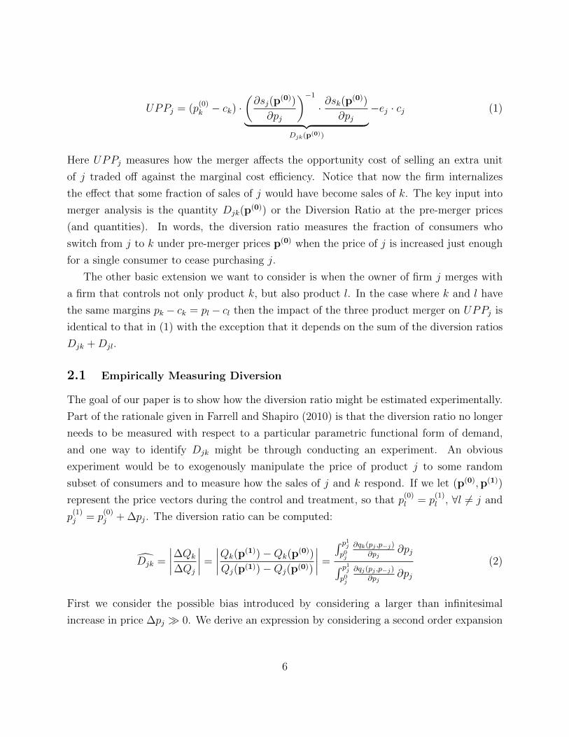
Here UPPj measures how the merger affects the opportunity cost of selling an extra unit

of j traded off against the marginal cost efficiency. Notice that now the firm internalizes

the effect that some fraction of sales of j would have become sales of k. The key input into

merger analysis is the quantity Djk(p(0)) or the Diversion Ratio at the pre-merger prices

(and quantities). In words, the diversion ratio measures the fraction of consumers who

switch from j to k under pre-merger prices p(0) when the price of j is increased just enough

for a single consumer to cease purchasing j.

The other basic extension we want to consider is when the owner of firm j merges with

a firm that controls not only product k, but also product l. In the case where k and l have

the same margins pk − ck = pl − cl then the impact of the three product merger on UPPj is

identical to that in (1) with the exception that it depends on the sum of the diversion ratios

Djk +Djl.

2.1 Empirically Measuring Diversion

The goal of our paper is to show how the diversion ratio might be estimated experimentally.

Part of the rationale given in Farrell and Shapiro (2010) is that the diversion ratio no longer

needs to be measured with respect to a particular parametric functional form of demand,

and one way to identify Djk might be through conducting an experiment. An obvious

experiment would be to exogenously manipulate the price of product j to some random

subset of consumers and to measure how the sales of j and k respond. If we let (p(0),p(1))

represent the price vectors during the control and treatment, so that p(0)l = p

(1)l , ∀l 6= j and

p(1)j = p

(0)j + ∆pj. The diversion ratio can be computed:

Djk =

∣∣∣∣∆Qk

∆Qj

∣∣∣∣ =

∣∣∣∣Qk(p(1))−Qk(p

(0))

Qj(p(1))−Qj(p(0))

∣∣∣∣ =

∫ p1jp0j

∂qk(pj ,p−j)

∂pj∂pj∫ p1j

p0j

∂qj(pj ,p−j)

∂pj∂pj

(2)

First we consider the possible bias introduced by considering a larger than infinitesimal

increase in price ∆pj � 0. We derive an expression by considering a second order expansion

6

of demand at p(0):

qk(p + ∆pj) ≈ qk(p) +∂qk∂pj

∆pj +∂2qk∂p2

j

(∆pj)2 +O((∆pj)

3)

qk(p + ∆pj)− qk(p)

∆pj≈ ∂qk

∂pj+∂2qk∂p2

j

∆pj +O(∆pj)2 (3)

This allows us to compute an expression for the bias in Djk:

Bias(Djk) ≈Djk

∂2qj∂p2j− ∂2qk

∂p2j

∂qj∂pj

+∂2qj∂p2j

∆pj∆pj (4)

Our expression in (4) shows that the bias of our diversion estimate depends on two things:

one is the magnitude of the price increase ∆pj, the second is the curvature of demand∂2qk∂p2j

. This suggests that bias is minimized by experimental designs that consider small price

changes. However, small changes in price may lead to noisy measures of ∆q. More formally

we assume constant diversion ∆qk ≈ Djk∆qj and construct a measure for the variance of the

diversion ratio:

V ar(Djk) ≈ V ar

(∆qk|∆qj|

)≈ 1

∆q2j

(D2jkσ

2∆qj

+ σ2∆qk− 2Djkρσ∆qjσ∆qk

)(5)

This implies a bias-variance tradeoff when estimating diversion. If our primary concern is

that the curvature of demand is steep, it suggests considering a small price increase. However,

if our primary concern is that sales are highly variable, we should consider a larger price

increase.

Instead of viewing our experiment as a biased measure of the marginal treatment effect,

we can instead ask: “What quantity does our experimental diversion measure estimate?”

We can derive an approximate relationship for our experimental diversion measure EDjk:

EDjk =1

∆qj

∫ p0j+∆p1

p0j

∂qk∂qj︸︷︷︸Djk(p)

∣∣∣∣∂qj∂pj

∣∣∣∣ ∂pj (6)

Thus an experiment varying the price pj measures the weighted average of diversion ratio,

where the weights correspond to the lost sales of j at a particular pj as a fraction of all lost

sales of j.

7

The experiments in our empirical example do not employ actual price changes, instead

the focal product is removed from the consumer’s choice set. This is equivalent to increasing

the price pj to the choke price where qj(pcj,p

(0)−j ) = 0. This has the advantage that it

minimizes the variance expression in (5). The other derivations in this section provide

insight in to when a product removal provides an accurate measure of diversion: (a) when

the curvature of demand is small (∂2qk∂p2j≈ 0), (b) when the true diversion ratio is constant

(or nearly constant) Djk(p) = Djk, or (c) when demand for j is steepest near the market

price

∣∣∣∣∂qj(pj ,p(0)−j )

∂pj

∣∣∣∣ � ∣∣∣∣∂qj(pj+δ,p(0)−j )

∂pj

∣∣∣∣.In our example, it might seem reasonable that customers who substitute away from a

Snickers bar after a five cent price increase switch to Reese’s Peanut Butter Cup at the

same rate as after a 25 cent price increase, where the only difference is the number of overall

consumers leaving Snickers. However in a different industry, this may no longer seem as

reasonable. For example, we might expect buyers of a Toyota Prius to substitute primarily

to other cheap, fuel-efficient cars when faced with a small price increase (from the market

price of $25,000 to $25,500), but we might expect substitution to luxury cars when facing

a larger price increase (from $45,000 to $45,500). Again, if demand (in units) for the Prius

falls rapidly with a small price increase, so that residual demand (and the potential impact

of further price increases) are small, then an experiment that considers removing it from the

choice set may provide an accurate measure of diversion, even though the diversion ratio

itself is not constant.

In the Appendix we derive explicit relationships for the Diversion Ratio for several well

known parametric demand functions. The important result is that both linear demand, and

the IIA logit demand model exhibit constant diversion ratios that do not vary with prices.

We also show that random coefficients logit demand, and CES demands (including log-linear

demand) do not generally exhibit constant diversion.

3 Description of Data and Industry

Globally, the snack foods industry is a $300 Billion a year business, compromised of a

number of large well-known firms and some of the most heavily advertised global brands.

Mars Incorporated reported over $50 Billion in Revenue in 2010, and represents the third

largest privately held firm in the US; other substantial players include Hershey, Nestle, Kraft,

Kellogg, Frito-Lay division of PepsiCo. While the snack-food industry as a whole might not

appear highly concentrated, sales within product categories can be very concentrated. For

8

example, Frito-Lay comprises around 40% of all savory snack sales in the United States,

and reported over $13 Billion in US revenues last year, but it’s sales outside the salty-snack

category are minimal, coming mostly through parent PepsiCo’s Quaker Oats brand and the

sales of Quaker Chewy Granola Bars.1

Over the last 25 years, the industry has been characterized by a large amount of merger

and acquisition activity, both on the level of individual brands and entire firms. For exam-

ple, the Famous Amos cookie brand has been owned by the Kellogg Company since 2001.

Between 1985 and 2001, Famous Amos cookies were owned by at least seven firms, including

the Keebler Cookie Company (acquired by Kellogg in 2001), Presidential Baking Company

(acquired by Keebler in 1998), as well as by other snack food makers and private equity firms.

Zoo Animal Crackers have a similarly complicated history owned by cracker manufacturer

Austin Quality Foods; before they too were acquired by the Keebler Cookie Co. (who in

turn was acquired by Kellogg).2

Our study measures diversion through the lens of a single medium-sized retail vending

operator in Chicago metropolitan area, MarkVend. Each of MarkVend’s machines internally

records price and quantity information. The data track total vends and revenues since the

last service visit on an item-level basis (but do not include time-stamps for each sale). Any

given machine can carry roughly 35 products at one time, depending on configuration. We

observe retail and wholesale prices for each product at each service visit during our 38-month

panel. There is relatively little price variation within a site, and almost no price variation

within a category (e.g., chocolate candy) at a site. This is helpful from an experimental

design perspective, but can pose a challenge to demand estimation. Very few “natural”

stock-outs occur at our set of machines.3 Most changes to the set of products available

to consumers are a result of product rotations, new product introductions, and product

retirements. Over all sites and months, we observe 185 unique products. We consolidate

some products with very low levels of sales using similar products within a category produced

by the same manufacturer, until we are left with the 73 ‘products’ that form the basis of the

1Most analysts believe Pepsi’s acquisition of Quaker Oats in 2001 was unrelated to its namesake businessbut rather for Quaker Oats’ ownership of Gatorade, a close competitor in the soft drink business.

2A landmark case in market definition was brought by Tastykake in attempt to block the acquisitionof Drake (the maker of Ring-Dings) by Ralston-Purina’s Hostess brand (the maker of Twinkies). Thatcase established the importance of geographically significant markets, as Drake’s had only 2% marketsharenationwide but a much larger share in the Northeast (including 50% of the New York market). Tastykakealso successfully argued that the relevant market was single-serving snack cakes rather than a broad categoryof snack foods involving cookies, candy bars. [Tasty Baking Co. v. Ralston Purina, Inc., 653 F. Supp. 1250- Dist. Court, ED Pennsylvania 1987]

3Mark Vend commits to a low level of stock-out events in its service contracts.

9

rest of our exercise.4

In addition to the data from Mark Vend, we also collect data on the characteristics of

each product online and through industry trade sources.5 For each product, we note its

manufacturer, as well as the following set of product characteristics: package size, number

of servings, and nutritional information.6

3.1 Experimental Design

We ran four experimental treatments with the help of the Mark Vend Company. These

represent a subset of a larger group of experiments we have used in other projects, such as

Conlon and Mortimer (2013). Our experiments followed a subset of Mark Vend’s operation,

60 snack machines located in professional office buildings, for which demand was historically

quite stable.7 Most of the customers at these sites are ‘white-collar’ employees of law firms

and insurance companies. Our goal in selecting the machines was to choose machines that

could be analyzed together, in order to be able to run each experiment over a shorter period

of time across more machines.8 Finally, we selected machines on routes that were staffed by

experienced drivers, so that the implementation of the experiments would be successful. The

60 machines used for each experiment were distributed across five of Mark Vend’s clients,

which had between 3 and 21 machines each. The largest client had two sets of floors serviced

on different days, and we divided this client into two sites. Generally, each site is spread

across multiple floors in a single high-rise office building, with machines located on each

floor.

For each experiment, we removed a product from all machines at a client site for a period

of 2.5 to 3 weeks. We conducted four experiments. In two of the experiments we removed

the two best-selling products from chocolate maker Mars Incorporated (Snickers and Peanut

M&Ms’), in another we removed the two best-selling products from the salty snack category

(PepsiCo’s: Doritos Nacho Cheese and Cheetos Crunchy); and for our third and fourth

4For example, we combine Milky Way Midnight with Milky Way, and Ruffles Original with Ruffles SourCream and Cheddar.

5For consolidated products, we collect data on product characteristics at the disaggregated level. Thecharacteristics of the consolidated product are computed as the weighted average of the characteristics ofthe component products, using vends to weight. In many cases, the observable characteristics are identical.

6Nutritional information includes weight, calories, fat calories, sodium, fiber, sugars, protein, carbohy-drates, and cholesterol.

7More precisely, demand at these sites is “relatively” stable compared to the population of sites servicedby the vending operator.

8Many high-volume machines are located in public areas (e.g., museums or hospitals), and have demand(and populations) that varies enormously from one day to the next, so we did not use machines of thisnature. In contrast, the work-force populations at our experimental sites are relatively homogenous.

10

experiment we removed two products owned by Kellogg’s: Famous Amos Chocolate Chip

Cookies, and Zoo Animal Crackers. We chose to run these two experiments separately in

part because the Animal Crackers are a difficult to categorize product; and close substitutes

are less obvious.

Whenever a product was experimentally stocked-out, poster-card announcements were

placed at the front of the empty product column. The announcements read “This product is

temporarily unavailable. We apologize for any inconvenience.” The purpose of the card was

two-fold: first, we wanted to avoid dynamic effects on sales as much as possible, and second,

the firm wanted to minimize the number of phone calls received in response to the stock-out

events. The dates of the interventions range from June 2007 to September 2008, with all

removals run during the months of May - October. We collected data for all machines for

just over three years, from January of 2006 until February of 2009. During each 2-3 week

experimental period, most machines receive service visits about three times. However, the

length of service visits varies across machines, with some machines visited more frequently

than others.

The cost of the experiment consisted primarily of driver costs. Drivers had to spend

extra time removing and reintroducing products to machines, and the driver dispatcher had

to spend time instructing the drivers, tracking the dates of each experiment, and reviewing

the data as they were collected. Drivers are generally paid a small commission on the

sales on their routes, so if sales levels fell dramatically as a result of the experiments, their

commissions could be affected. Tracking commissions and extra minutes on each route for

each driver would have been prohibitively expensive to do, and so drivers were provided with

$25 gift cards for gasoline during each week in which a product was removed on their route

to compensate them for the extra time and the potential for lower commissions. With the

exception of an individual site in one treatment, implementation was successful.9

Our experiment differs somewhat from an ideal experiment. Ideally, we would be able to

randomize the choice set on an individual level, though technologically that is difficult in both

vending and traditional brick and mortar contexts. In contrast, online retailers are capable

of showing consumers different sets of products and prices simultaneously. This leaves our

design susceptible to contamination if for example, Kraft runs a large advertising campaign

for Planters Peanuts that corresponds to the timing of one of our experiments. Additionally,

because we remove all of the products at an entire client site for a period of 2.5 to 3 weeks,

9In the unsuccessful run, the driver at one site forgot to remove the focal product, so no intervention tookplace.

11

we lack a contemporaneous group of untreated machines. We chose this design, rather than

randomly staggering the product removals, because we (and the participating firms) were

afraid consumers might travel from floor to floor searching for stocked out products. This

design consideration prevents us from using control machines in the same building, and

makes it more difficult to capture weekly variation in sales due to unrelated factors, such as

a law firm taking a big case to trial, or accountants during quarterly reporting season. In

balance, we thought that people traveling from floor to floor was a larger concern. It also

has the additional benefit that we can aggregate over all machines at a client site, and treat

the entire site as if it were a single machine.

4 Analyses of the Experimental Outcomes

4.1 Paired Differences

One goal of our experiment is to determine how sales are diverted away from best-selling

products. All of these data are recorded at the level of a service visit to a vending machine.

Because machines are serviced on different schedules it is sometimes more convenient to

organize observations by week, rather than by visit. When we do this, we assume that

sales are distributed uniformly among the business days in a service interval, and assign

those to weeks. Because different experimental treatments start on different days of the

week, we allow our definition of when weeks start and end to depend on the client site

and experiment.10 The next step we take is to aggregate our data to the level of a client

site-week rather than a machine-week. We do this for two reasons, the first is that sales

at the individual machine level are quite small and can vary quite a bit over time. This

would make it hard to measure any kind of effect. The second is that we don’t want to

worry about consumers going from machine to machine searching for missing products, or

additional noise in demand created by a long meeting on a particular floor, etc.

Let’s begin by defining some basic quantities. We let qjt denote the sales of product j in

site-week t, and we use a superscript 1 to denote sales when a focal product(s) is removed,

and a superscript 0 to denote sales when a focal product(s) is available. We denote the set of

available products as A, and F as the set of products we remove for our experiment. Then

Q1t =

∑j∈A\F q

1jt and Q0

s =∑

j∈A q0js are the overall sales during a treatment week, and

control week respectively. It is also convenient to write the sales of the removed products

q0fs =

∑j∈F q

0js. Our goal is to compute ∆qkt = q1

kt−E[q0kt], the treatment effect on the sales

10At some site-experiment pairs, weeks run Tuesday to Monday, while others run Thursday to Wednesday.

12

of product k of the experiment, and the diversion ratio Dfs,k = ∆qktq0fs

. In the context of our

experiment, the diversion ratio has a simple interpretation: the change in sales for product k

during our experiment as a fraction of sales of the focal product(s) during the control period.

In principle, this calculation is straightforward. In practice, however, there are two

challenges in implementing the experiments and interpreting the data generated by them.

The first challenge is that there is a large amount of variation in overall sales at the weekly

level independent of our experiments. This weekly variation in overall sales is common in

retail environments. It is not uncommon for week over week sales to vary by over 20%, while

no single product enjoys more than 4.5% market share. This can be seen in Figure 1 which

plots the overall sales of all machines from one of the sites in our sample on a weekly basis.

For example, a law firm may have a large case going to trial in a given month, and vend

levels will increase at the firm during that period. In our particular setting, many of the

experiments were run during the summer of 2007, which was a high-point in demand at these

sites, most likely due to macroeconomic conditions. In this case, using a simple measure like

previous weeks’ sales, or overall average sales for E[q0jt] could result in unreasonable treatment

effects, such as sales increasing due to stock-out events, or sales decreasing by more than the

sales of the focal products.

We deal with this challenge by imposing a simple restriction born out of consumer theory.

After we have aggregated our data across machines to the level of a client-week observation,

we restrict the set of possible control weeks, so that aggregate sales do not increase as the

result of our experiment. Likewise, we also impose that aggregate sales do not decline by

more than the sales of the product we removed. Mathematically the set of control weeks s

corresponding to treatment week t is defined by:

{s : s 6= t, Q0t −Q1

s ∈ [0, q0fs]} (7)

Notice that this is the same as placing a restriction on the sum of the diversion ratios:∑j∈A\F

Dfs,j ∈ [0, 100%] (8)

While this has the nice property that it imposes the restriction on our selection of control

weeks that all products are weak-substitutes, it has the disadvantage that it introduces the

potential for selection bias. The bias results from the fact that weeks with unusually high

sales of the focal product q0fs are now more likely to be included in our control. Because it

13

would make the denominator too large, the bias would likely understate the diversion ratio.

We propose a slight modification of (7) which removes the bias. That is, we can replace

q0fs with q0

fs = E[q0fs|Q0

s]. An easy way to obtain the expectation is to run an OLS regression

of q0fs on Q0

s (for the subsample where focal products are available), at the machine level and

use the predicted value. This has the nice property that the error is orthogonal to Q0s, which

ensures that our choice of weeks is now unbiased. We run one regression for each client-site

and report the results for one of the client-sites in Table 1.

We use our definition of control weeks s to compute the expected control sales that

correspond to treatment week t as:

St = {s : s 6= t, Q0t −Q1

s ∈ [0, b0 + b1Q0s]} (9)

The second challenge is that, although the experimental design is relatively clean, the product

mix presented in a machine is not necessarily fixed across machines, or within a machine

over long periods of time because we rely on observational data for the control weeks. For

example, manufacturers may change their product lines, or Mark Vend may change its

stocking decisions over time). Thus while our experiments intend to isolate the treatment

effect of removing Snickers and M&M Peanut, we might instead compute the treatment

effect of removing the Mars products jointly with changing pretzel suppliers. There are two

possible options to mitigate this problem. The first would be to further restrict the set of

potential control weeks so that control weeks had similar availability to our experimental

weeks (at least among some subset of products). If we were considering one specific merger,

it would make sense to focus our attention so that the set of available products was the

same during treatment and control for the two merging firms. For example, if 3 Musketeers

was unavailable during our Mars experiment, we would restrict our control weeks only to

weeks where 3 Musketeers was also unavailable. This removes some contamination where

substitution from 3 Musketeers to Reese’s Peanut Butter Cups is also attributed to diversion

from Snickers and M&M Peanut. The disadvantage of this approach is that as we want to

control more carefully for the set of available products, we reduce the number of potential

control weeks.

An alternative approach is to adjust the product assortment from the control period to

correspond to the product assortment in the treatment period. We do this by computing

the percentage of consumers who would have seen the product available when making their

purchase for the treatment and control period. For each machine, and each week we deter-

mine which products were available and then weight each week by it’s corresponding sales at

14

the machine-level to form a consumer-weighted average level of availability at the site-week

level. Thus busier machines and busier weeks are given more weight than less busy ones.

This should roughly correspond to the probability that a randomly sampled consumer sees a

product available for purchase. We construct this measure which we call “% Availability” for

both treatment and control periods.11. We then use the ratio %Avail1%Avail0

to rescale the control

vends to correspond to the availability during the treatment period.

The basic idea of the approach is as follows. If during the treatment period Reese’s

Peanut Butter Cups was available during 75% of sales-weighted machine-weeks, and during

the control it was available during 25% of sales-weighted machine weeks, then even without

any change in the availability of the focal products, we might expected a threefold increase in

the sales of Reese’s Peanut Butter Cups ; therefore we multiply our observed control vends by%Avail1%Avail0

= 3 and use that to compute the change in vends. Likewise, a product that had 25%

availability during the treatment period, but was available for 50% of the time during the

control period would be adjusted so that V ends0 was half as large. This avoids the problem of

computing negative diversion just because products were less likely to be available during the

treatment than during the control. This adjustment only addresses changes in “own product”

availability. It does not account for the fact that sales of Reese’s Peanut Butter Cups might

increase because availability of a close competitor such as 3 Musketeers was reduced during

the control period, and still attributes all of those sales to the effect of the experiment. The

results of these adjustments are reported in Table 3 for the subset of products with positive

diversion for the Mars experiment.12. While this adjustment addresses changes in availability

of substitute products, it no longer gets the aggregate diversion patterns correct. Even with

our restriction on control weeks in (9), after the adjustments we can get diversion ratios

that are less than zero or greater than 100% in aggregate. Therefore we rescale the adjusted

change in vends for products with positive diversion by a constant (experiment-specific)

factor, γ, for all products so that the aggregate diversion ratio is the same before and after

our availability adjustment. This is demonstrated in Table 2.

When we review Table 3 we see that the adjustments are generally quite small, as avail-

ability is roughly the same during the treatment and control weeks. Though in a few cases

the adjustment is crucial. For example, Reese’s Peanut Butter Cups is a close competitor

to the two Mars products Snickers and Peanut M&M’s and sees the largest change in un-

adjusted sales. After the adjustment, the change in sales is considerably smaller (33.4 units

11When we compute % Availability for control periods, we use the sales at the corresponding treatmentweeks as determined by (9), rather than the sales at the control weeks themselves.

12The full set of adjustments for all product and all experiments are available in an online appendix.

15

instead of 118.2 units) but still quite substantial. Similarly, Salty Other shows a negative

change in sales as a result of the Mars experiment implying that it is a complement rather

than a substitute, but after adjusting for declining availability the sign changes.

And for each treatment week t we can compute the treatment effect and diversion ratio

as:

∆qkt = q1kt −

AV(1)k

AV(0)k

· γ

#St

∑s∈St

q0ks (10)

Djk =∆qkt

q(0)jt

(11)

Once we have constructed our restricted set of treatment weeks and the set of control weeks

that corresponds to each, inference is fairly straightforward. We use (10) to construct a set

of pseudo-observations for the difference, and employ a t-test for differences.

4.2 Regression Based Approach

An alternative to the paired differences specification presented above, is to consider a re-

gression based identification strategy for measuring diversion. Begin with data on the sales

of each product j in week t and machine m:

qjmt = αjm + βj × treatmentmt + εjmt (12)

In this specification αjm is a product-machine specific intercept, and βj is the effect the

experiment has on the sales of j. Just like in the paired-differences setup we face two major

challenges when identifying βj. The first is that the level of overall sales varies quite a

bit within machines from week to week. The second is that the availability of other (non-

experimental) products may be correlated with our treatment. To deal with the second

problem, we can include indicator variables for the availability of other products as controls,

we label these coefficients γjk. To control for the overall sales level, we might like to include

week specific fixed effects, however those would be collinear with our treatment. Instead we

could consider interacting all of our right hand side variables with the a control for the size

of the market at machine m in week t, Mmt. We can just rescale qjmt by Mmt and work with

the marketshare sjmt instead of the quantity:

sjmt ≡qjmtMmt

= αjm + βj × treatmentmt +∑k

γjk × availkmt + εjmt (13)

16

Under this specification we construct the expected change in sales of k, and the corresponding

diversion ratio implied by the experiment:

E[∆qk] = βk × I[βk ≥ 0]×∑

(m,t):k∈Am,t

Mmt (14)

Djk =E[∆qk]

E[∆qj]

In words, after computing the treatment effect βk in marketshare terms, we compute diver-

sion by predicting the change in quantity for each machine-week for which k is available,

and divide that by the overall sales of the focal product across our dataset. We use the

historical maximum weekly sales at the machine level as the market size. We can construct

our diversion measure over just the treatment weeks (which corresponds to the paired dif-

ferences result of the previous section), or all of the weeks in our observational data (which

corresponds to the parametric models of the next section). One advantage that this regres-

sion based approach may have over the paired differences is that we are able to incorporate

controls for βk while still utilizing the entire dataset.

4.3 Parametric Specifications

In addition to computing treatment effects, we also specify two parametric models of de-

mand: nested logit and random-coefficients logit, which are estimated from the full dataset

(including weeks of observational data that do not meet any of our control criteria).

We consider a model of utility where consumer i receives utility from choosing product

j in market t of:

uijt = δjt + µijt + εijt (15)

The parameter δjt is a product-specific intercept that captures the mean utility of product

j in market t, and µijt captures individual-specific correlation in tastes for products.

In the case where (µijt + εijt) is distributed generalized extreme value, the error terms

allow for correlation among products within a pre-specified group, but otherwise assume no

correlation. This produces the well-known nested-logit model of McFadden (1978) and Train

(2003). In this model consumers first choose a product category l composed of products gl,

and then choose a specific product j within that group. The resulting choice probability for

17

product j in market t is given by the closed-form expression:

pjt(δ, λ, at) =eδjt/λl(

∑k∈gl∩at e

δkt/λl)λl−1∑∀l(∑

k∈gl∩at eδkt/λl)λl

(16)

where the parameter λl governs within-group correlation, and at is the set of available prod-

ucts in market t.13

The random-coefficients logit allows for correlation in tastes across observed product char-

acteristics. This correlation in tastes is captured by allowing the term µijt to be distributed

according to f(µijt|θ). A common specification is to allow consumers to have independent

normally distributed tastes for product characteristics, so that µijt =∑

l σlνiltxjl where

νilt ∼ N(0, 1) and σl represents the standard deviation of the heterogeneous taste for prod-

uct characteristic xjl. The resulting choice probabilities are a mixture over the logit choice

probabilities for many different values of µijt, shown here:

pjt(δ, θ, at) =

∫eδjt+

∑l σlνiltxjl

1 +∑

k∈at eδkt+

∑l σlνiltxkl

f(ν)d ν (17)

Estimation then proceeds by full information maximum likelihood (FIML) in the case of

nested logit or maximum simulated likelihood (MSL) in the case of the random coefficients.

The log-likelihood is:

θMLE = arg maxθ

∑j,t

qj,t log(pjt(δ, θ; at))

In both the nested-logit and random-coefficient models we let δjt = dj+ξt, that is we separate

mean utility into a product intercept and a market specific demand shifter. We include an

additional ξt for each of our 15,256 machine-visits, or 2710 unique choice sets. For the

nested-logit model, we allow for heterogeneous tastes across five major product categories

or nests: chocolate candy,non-chocolate candy, cookie, salty snack, and other.14 For the

random-coefficients specification, we allow for three random coefficients, corresponding to

13Note that this is not the IV regression/‘within-group share’ presentation of the nested-logit model inBerry (1994), in which σ provides a measure of the correlation of choices within a nest. Roughly speaking,in the notation used here, λ = 1 corresponds to the plain logit, and (1 − λ) provides a measure of the‘correlation’ of choices within a nest (as in McFadden (1978)). The parameter λ is sometimes referred to asthe ‘dissimiliarity parameter.’

14The vending operator defines categories in the same way. “Other” includes products such as peanuts,fruit snacks, crackers, and granola bars.

18

consumer tastes for salt, sugar, and nut content.15

We provide information on how to calculate diversion ratios under these parametric

models in the Appendix. An important decision is how to determine the choice set used

in the counterfactual prediction exercise. We use a single choice set based on the most

commonly available products during our treatment period. An alternative would be to

consider a representative choice set based on some other period, or to predict the change

in vends for each market observed in the data and then aggregate to obtain a choice-set

weighted diversion prediction (similar to how we construct the OLS prediction). We choose

the simpler representative choice set, because we believe it better approximates the approach

likely to be taken by empirical researchers.

4.4 Identification and Parameter Estimates

The treatment effects approach and the parametric model rely on two different sources of

identification. Formal nonparametric identification results for random utility models such

as Berry and Haile (2010) or Fox and Gandhi (2012) often rely on variation across markets

in continuous characteristics such as price. This is unavailable in the vending setting, since

there is little to no price variation. Instead, the parametric models are identified through

discrete changes in the choice set, primarily through product rotations. The intuition is

that Snickers and Milky Way may look similar in terms of observable characteristics (a

Snickers is essentially a Milky Way with peanuts), but have different marketshares. In fact,

Snickers often outsells Milky Way 3:1 or better, this leads us to conclude that Snickers offers

higher mean utility to consumers. At the same time, sales may respond differently to the

availability of a third product. For example, if Planters Peanuts is introduced to the choice

set, and it reduces sales of Snickers relatively more than Milky Way we might conclude there

are heterogeneous preferences for peanuts. One challenge of this approach, is that while we

might observe many differences in relative substitution patterns across products, we must

in essence project them onto a lower dimensional basis of random coefficients. Thus if our

model did not include a random parameter for peanuts, we would have to explain those

15We do not allow for a random coefficient on price because of the relative lack of price variation in thevending machines. We also do not include random coefficients on any discrete variables (such as whetheror not a product contains chocolate). As we discuss in Conlon and Mortimer (Forthcoming), the lack ofvariation in a continuous variable (e.g., price) implies that random coefficients on categorical variables maynot be identified when product dummies are included in estimation. We did estimate a number of alternativespecifications in which we include random coefficients on other continuous variables, such as carbohydrates,fat, or calories. In general, the additional parameters were not significantly different from zero, and theyhad no appreciable effect on the results of any prediction exercises.

19

tastes with something else, like “salt”.

In the absence of experimental variation, many of the best-selling products are essentially

always stocked by the retailer. Therefore we learn about how closely popular products

compete primarily through how marketshares respond to the availability of a third often much

less popular product. The identifying variation comes through the fact that we observe 2,710

different choice sets in 15,256 service visits. If for example, all machines stocked exactly the

same set of products every week, we would only have a single choice set, and would struggle

to identify nonlinear parameters.16

While the product rotations are crucial to the identification of the parametric models,

they are somewhat of a nuisance to the identification of the treatment effects model. Product

rotations introduce additional heterogeneity that must either be specifically controlled for,

or risks introducing bias into the estimated treatment effect. The ideal identification setting

for the treatment effect would be if there were no non-experimental variation in either prices

or the set of available products. Thus the treatment effect estimator should perform best

precisely when we worry the parametric demand model may not be identified and vice versa.

This creates an inherent problem in any setting where the two approaches are pitted head

to head in a “horse race” scenario.

Both the treatment effects approach and the discrete choice models benefit from exper-

imental variation in the choice set. Because we consider diversion from popular products,

there are very few cases “in the wild” where these items are not in stock. Thus, in the absence

of experimental variation, the parametric model forecasts the effect of removing Snickers

from how its sales are reduced when Reese’s Peanut Butter Cups (or some other substitute)

were present. Obviously, with experimental variation this becomes an “in-sample” prediction

exercise for the parametric model.

In Tables 4 and 5, we report the parameter estimates for our preferred specification of

the random coefficients and nested logit models. We considered a large number of alterna-

tive models, but presented the results selected by the Bayesian Information Crtieria (BIC).

All of our estimates included 73 product-specific intercepts. In the case of the nested logit

model, this included 5 nests (Chocolate, Non-Chocolate Candy, Cookie/Pastry, SaltySnack,

and Other). For the random coefficients model, this included only three normally distributed

random coefficients (Salt, Sugar, and Nut Content), though we considered additional specifi-

cations including coefficients on Fat, Calories, Chocolate, Protein, Cheese, and other product

characteristics. Additionally we estimated both sets of models with both choice set fixed

16Typically this problem could be alleviated by seeing variation in prices within a product over time.

20

demand shifters ξt and machine-visit level demand shifters. While the extra demand shifters

improved the fit, BIC preferred the smaller set of fixed effects.

To further explore the identification issues, we estimated each specification excluding the

data from different experiments one at a time, and another where excluded all treatment

periods. The results are clearest in the nested logit model. In that model all of the non-

linear parameters λ increase in magnitude. As λ represents the dissimilarity parameter of

McFadden (1978), where 0 is perfect correlation within the nest and λ→ 1 implies IIA logit

substitution; this implies that without experimental variation there is less within nest cor-

relation and the nested logit behaves more logit-like. This means that without experimental

variation, the nested logit model would predict diversion patterns that would be explained

mostly by ex-ante marketshares and less by the grouping of products. The results for the

random coefficient model are less obvious, as withholding experimental variation leads to

more heterogenous tastes for nuts but no statistically significant heterogeneous tastes for

sugar.

5 Results

Our primary goal has been both to show how to measure diversion ratios experimentally, but

also to understand how those experimentally measured diversion ratios compare to diversion

ratios obtained from common parametric models of demand.

Table 6 shows the diversion computed for the top 5 substitutes under the treatment

effects approach and the diversion computed under random coefficients, and nested logit

models for each experiment. There is a general pattern that emerges. The logit-type models

and the treatment effects approach predict a similar order for substitutes (i.e.: the best

substitute, the second best substitute, and so on). Also, they tend to predict similar di-

version ratios for the third, fourth and fifth best substitute. For example in the Snickers

and M&M Peanut experiment, the treatment effects approach and the random coefficients

logit approach predict around 4% diversion to Reese’s Peanut Butter Cups and M&M Milk

Chocolate. However, there tends to be a big discrepancy across all experiments for the diver-

sion to the best-substitute product. The treatment effect predicts nearly 14.2% of consumers

substituting to Twix, while the random coefficients model predicts only 6.4%. This effect is

large enough that it could lead to incorrect conclusions about upward pricing pressure or a

potential merger.

It is important to point out that our results should not be interpreted as showing that

the treatment effects approach is always preferred to the parametric demand estimation

21

approach. In the Famous Amos Cookie experiment, the treatment effect shows that 20.7%

of consumers switch from Famous Amos Chocolate Chip Cookies to Sun Chips, while the

random coefficient model predicts diversion < 1% (the products quite dissimilar). While this

effect appears large in the raw data, it represents an effect that most industry experts would

be unlikely to believe. Moreover, the effect is not precisely estimated as indicated by table

7. In part this may be because we have imperfectly adjusted for increased availability of Sun

Chips, or because we have failed to adjust for some close competitor of Sun Chips, or that

overall sales levels of Sun Chips are highly variable.17 While the parametric demand models

observe the reduced availability of Smartfood Popcorn and use that to improve its estimates

of parameters, the treatment effects model is now faced with confounding variation.

Table 7 shows diversion ratios aggregated to the level of a manufacturer. The results

exhibit the same pattern as before where the treatment effects predict much more substi-

tution to the closest substitutes than the random coefficients and nested logit models do.

In some sense, for merger analysis, correctly predicting diversion to one or two closest sub-

stitutes might be the most important feature of a model or identification strategy, since

those are the potential mergers we should be most concerned about. The other potential

anomaly is that after adjusting for product availability, the aggregate diversion measures

from the paired differences approach can be unrealistically high (> 240%). In the columns

labeled “Adj. Differences” and “Adj. OLS” we re-scale all of the diversion estimates, so that

the aggregate diversion (among manufacturers with positive diversion) matches the original

aggregate diversion in the paired (but unadjusted for availability) data. Much of the differ-

ences between the parametric models and the treatment effects approach can be attributed

to substitution to the outside good. The parametric models predict that consumers will be

diverted to some other product at rate of approximately 30-45%, while the paired and OLS

approaches predict that consumers will be diverted at a rate of 65-75%. All of the models

broadly predict the same relative magnitudes, but the parametric models predict smaller

aggregate magnitudes. A different parametrization of the outside share, might lead to more

similar estimates.

In table 8 we compute the gross upward pricing pressure index (GUPPI). Guppi is

GUPPIj = Djkpk−ckpj

. Here we exploit the fact that we observe the wholesale contracts

17Imagine that our treatment weeks at our largest location are correlated with reduced availability ofSmartfood Popcorn for reasons unrelated to our experiment, such as supply problems at the warehouse (Itis!). In that case we could think about the actual experiment as removing Famous Amos Cookies andSmartfood Popcorn simultaneously, but the one we measure as attributing the entire effect to the FamousAmos Cookies.

22

between the retailer and the manufacturer, and let the wholesale price serve as pj, pk in the

above expression. We assume that all products have a manufacturing cost of $0.15, and

exploit the fact that within manufacturer-category there is no wholesale price variations:

(Snickers and 3 Musketeers have the same wholesale price even though one is much more

popular than the other). Under a symmetry assumption (not true in our example) the crit-

ical value for GUPPI is generally 10%, because it corresponds to SSNIP of 5% under the

hypothetical monopolist test. If we apply the same 10% threshold to our results we find

that a Mars-Hershey merger would likely attract further scrutiny, but not a Mars-Nestle

merger (at least not for the prices of Snickers and M&M Peanut). Meanwhile the acquisi-

tion of the Mars or Pepsi product portfolio might place upward pricing pressure on either

the Animal Crackers, as they exhibit large point estimates for GUPPI under the treatment

effects approach, though diversion is not statistically significant from zero, and the effects

are imprecise. Similarly the Famous Amos cookies show a large but imprecise point estimate

for the acquisition of the Pepsi portfolio (driven by an inexplicable rise in the sales of Sun

Chips).

6 Conclusion

Under the revised 2010 Horizontal Merger Guidelines, the focus on the diversion ratio and the

“single product merger simulation” approach in UPP and GUPPI where all other prices and

quantities are held fixed, imply that the diversion ratio serves as a single sufficient statistic

for at least the initial screening stage of merger evaluation. We show that the diversion

ratio has the attractive empirical property that it can be estimated via experimental or

quasi-experimental techniques in a relatively straightforward manner. Our hope is that this

makes a well-developed set of tools available both to IO researchers, and also to antitrust

practitioners.

At the same time, we are quick to point out that while the diversion ratio can be ob-

tained experimentally, it is not trivial, and researchers should think carefully about which

treatment effect their experiment (or quasi-experiment) is actually identifying; as well as

what identifying assumptions required for estimating the diversion ratio implicitly assume

about the structure of demand. An important characteristic of many retail settings is that

even category level sales are much more variable than most product level market shares.

We partially alleviate this problem by employing full removal of the product, rather than

marginal price increases, and derive conditions under which this may provide a reasonable

approximation to the marginal diversion ratio. Even under our design, the overall variabil-

23

ity in the sales levels can make diversion ratios difficult to measure. If the agencies were

to requires that firms submit to similar experiments as part of the merger review process,

they would likely incorporate prior information and focus experiments on a narrower set of

potential products than we considered in our setting.

Perhaps someday soon, potential mergers could even be evaluated by agreeing to an

experiment in lieu of lengthy and costly court proceedings.

24

References

Angrist, J., and J.-S. Pischke (2010): “The Credibility Revolution in Empirical Eco-nomics: How Better Research Design is Taking the Con out of Econometrics,” The Journalof Economic Perspectives, 24(2), 3–30.

Berry, S. (1994): “Estimating discrete-choice models of product differentiation,” RANDJournal of Economics, 25(2), 242–261.

Berry, S., and P. Haile (2010): “Nonparametric Identification of Multinomial ChoiceDemand Models with Heterogeneous Consumers,” Working Paper.

Carlton, D. W. (2010): “Revising the Horizontal Merger Guidelines,” Journal of Com-petition Law and Economics, 6(3), 619–652.

Chetty, R. (2009): “Sufficient Statistics for Welfare Analysis: A Bridge Between Structuraland Reduced-Form Methods,” Annual Review of Economics, 1(1), 451–488.

Cheung, L. (2011): “The Upward Pricing Pressure Test for Merger Analysis: An EmpiricalExamination,” Working Paper.

Conlon, C., and J. H. Mortimer (2013): “All Units Discount: Experimental Evidencefrom the Vending Industry,” Working Paper.

(Forthcoming): “Demand Estimation Under Incomplete Product Availability,”American Economic Journal: Microeconomics.

Einav, L., and J. Levin (2010): “Empirical Industrial Organization: A Progress Report,”The Journal of Economic Perspectives, 24(2), 145–162.

Farrell, J., and C. Shapiro (2010): “Antitrust Evaluation of Horizontal Mergers: AnEconomic Alternative to Market Definition,” The B.E. Journal of Theoretical Economics,10(1), 1–41.

Fox, J., and A. Gandhi (2012): “Nonparametric Identification and Estimation of RandomCoefficients in Nonlinear Economic Models,” Working Paper.

Fox, J. T., K.-i. Kim, S. P. Ryan, and P. Bajari (2011): “A Simple Estimator for theDistribution of Random Coefficients,” Quantitative Economics, 2(3), 381–418.

Hausman, J. A. (2010): “2010 Merger Guidelines: Empirical Analysis,” Working Paper.

Heckman, J. J. (2010): “Building Bridges Between Structural and Program EvaluationApproaches to Evaluating Policy,” Journal of Economic Literature, 48(2), 356–398.

Jaffe, S., and E. G. Weyl (Forthcoming): “The First Order Approach to Merger Anal-ysis,” American Economic Journal: Microeconomics.

25

Keane, M. (2010): “A Structural Perspective on the Experimentalist School,” The Journalof Economic Perspectives, 24(2), 47–58.

Leamer, E. (1983): “Let’s Take the Con Out of Econometrics,” American Economic Re-view, 75(3), 308–313.

(2010): “Tantalus on the Road to Asymptopia,” The Journal of Economic Per-spectives, 24(2), 31–46.

McFadden, D. (1978): “Modelling the Choice of Residential Location,” in Spatial Inter-action Theory and Planning Models, ed. by A. Karlqvist, L. Lundsqvist, F. Snickars, and

J. Weibull. North-Holland.

Miller, N. H., M. Remer, C. Ryan, and G. Sheu (2012): “Approximating the PriceEffects of Mergers:Numerical Evidence and an Empirical Application,” Working Paper.

Nevo, A. (2001): “Measuring Market Power in the Ready-to-Eat Cereal Industry,” Econo-metrica, 69, 307–342.

Nevo, A., and M. Whinston (2010): “Taking the Dogma out of Econometrics: StructuralModeling and Credible Inference,” The Journal of Economic Perspectives, 24(2), 69–82.

Reynolds, G., and C. Walters (2008): “The use of customer surveys for market defini-tion and the competitive assessment of horizontal mergers,” Journal of Competition Lawand Economics, 4(2), 411–431.

Schmalensee, R. (2009): “Should New Merger Guidelines Give UPP Market Definition?,”Antitrust Chronicle, 12, 1.

Sims, C. (2010): “But Economics Is Not an Experimental Science,” The Journal of Eco-nomic Perspectives, 24(2), 59–68.

Stock, J. (2010): “The Other Transformation in Econometric Practice: Robust Tools forInference,” The Journal of Economic Perspectives, 24(2), 83–94.

Train, K. (2003): Discrete Choice Methods with Simulation. Cambridge University Press.

Willig, R. (2011): “Unilateral Competitive Effects of Mergers: Upward Pricing Pressure,Product Quality, and Other Extensions,” Review of Industrial Organization, 39(1-2), 19–38.

26

600

800

1000

1200

1400

1600

0 50 100 150Week

TotalVends (mean) totalvends

Figure 1: Total Sales by Week, Site 93

27

Focal Sales β0 βtotalsales R2

Zoo Animal Cracker 6.424 0.039 0.503Famous Amos Cookie 6.937 0.025 0.395Doritos and Cheetos -16.859 0.078 0.628Snickers and Peanut M&Ms -1.381 0.127 0.704

Table 1: Selection of Control Weeks: Regression for Focal Sales at Site 93

Experiment Unadjusted Adjusted Adjusted (> 0) Rescaling FactorZoo Animal Cracker 77.35 84.58 246.11 0.31Famous Amos Cookie 65.30 -178.83 181.98 0.36Cheetos and Doritos 66.22 -7.57 101.62 0.65Snickers and Peanut M&M 66.47 17.69 79.00 0.84

Table 2: Selection of Control Weeks: Regression for Focal Sales at Site 93

28

Manufacturer Product V ends0 V ends1 (% Avail0) (% Avail1) Adjusted Control

Hershey Payday 1.2 6.6 1.3 2.5 2.3Hershey Reeses Peanut Butter Cups 56.5 174.7 29.0 72.5 141.3Hershey Twizzlers 24.3 57.3 17.7 37.0 50.7Hershey Choc Herhsey (Con) 37.2 65.9 29.9 35.5 44.2Kellogg Brown Sug Pop-Tarts 5.9 5.9 4.6 3.7 4.7Kellogg Strwbry Pop-Tarts 127.6 139.6 77.7 78.7 129.2Kellogg Cheez-It Original SS 190.0 206.2 84.6 82.3 184.8Kellogg Choc Chip Famous Amos 189.7 209.5 99.9 100.0 189.9Kellogg Rice Krispies Treats 26.1 82.7 30.7 60.8 51.7Kraft Ritz Bits Chs Vend 21.9 27.1 37.0 45.3 26.8Kraft 100 Cal Oreo Thin Crisps 32.4 46.9 25.3 33.5 42.8Mars M&M Milk Chocolate 113.2 144.6 61.0 57.6 106.7Mars Milky Way 17.0 64.3 17.9 26.9 25.5Mars Twix Caramel 182.7 301.4 78.6 80.0 186.0Mars Nonchoc Mars (Con) 33.3 44.5 26.1 25.2 32.2Nestle Butterfinger 41.3 61.8 31.3 31.8 41.9Nestle Raisinets 149.2 199.3 80.8 83.1 153.5Pepsi Frito LSS 160.7 187.1 75.6 78.9 167.8Pepsi Grandmas Choc Chip 78.9 83.7 55.3 52.0 74.2Pepsi Lays Potato Chips 1oz SS 117.8 181.2 53.5 78.8 173.5Pepsi Baked Chips (Con) 208.1 228.0 91.7 97.5 221.3Snyders Snyders (Con) 367.6 418.6 82.6 87.2 387.9Sherwood Ruger Wafer (Con) 116.6 151.9 63.7 80.9 148.1Kar’s Nuts Kar Sweet&Salty Mix 2oz 111.2 134.9 61.5 66.9 121.1Misc Rasbry Knotts 63.7 72.4 82.5 77.9 60.1Misc Farleys Mixed Fruit Snacks 66.6 78.8 57.3 67.4 78.3Misc Other Pastry (Con) 0.5 10.5 1.6 5.0 1.5Misc Salty Other (Con) 35.7 29.1 20.4 15.4 27.1

Table 3: Adjustments of Control Weeks: Mars (Snickers, Peanut M&M’s) Experiment

29

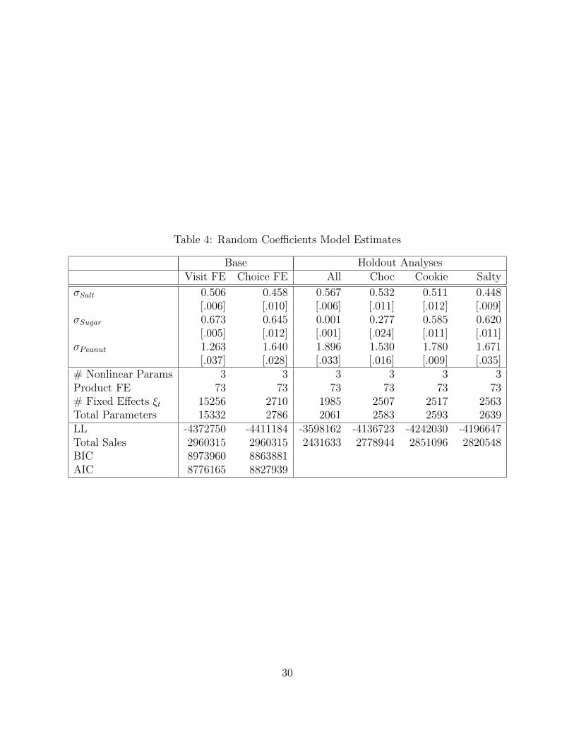
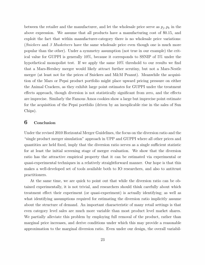
Table 4: Random Coefficients Model Estimates

Base Holdout AnalysesVisit FE Choice FE All Choc Cookie Salty

σSalt 0.506 0.458 0.567 0.532 0.511 0.448[.006] [.010] [.006] [.011] [.012] [.009]

σSugar 0.673 0.645 0.001 0.277 0.585 0.620[.005] [.012] [.001] [.024] [.011] [.011]

σPeanut 1.263 1.640 1.896 1.530 1.780 1.671[.037] [.028] [.033] [.016] [.009] [.035]

# Nonlinear Params 3 3 3 3 3 3Product FE 73 73 73 73 73 73# Fixed Effects ξt 15256 2710 1985 2507 2517 2563Total Parameters 15332 2786 2061 2583 2593 2639LL -4372750 -4411184 -3598162 -4136723 -4242030 -4196647Total Sales 2960315 2960315 2431633 2778944 2851096 2820548BIC 8973960 8863881AIC 8776165 8827939

30

Table 5: Nested Logit Model Estimates

Base Holdout AnalysesVisit FE Choice FE All Choc Cookie Salty

λChocolate 0.828 0.810 0.917 0.873 0.813 0.814[.003] [.005] [.006] [.005] [.005] [.005]

λCandyNon−Choc 0.908 0.909 0.947 0.916 0.918 0.910[.007] [.009] [.010] [.009] [.009] [.009]

λCookie/Pastry 0.845 0.866 0.933 0.901 0.869 0.874[.004] [.006] [.007] [.007] [.006] [.006]

λOther 0.883 0.894 0.937 0.926 0.895 0.897[.005] [.006] [.007] [.007] [.006] [.006]

λSaltySnack 0.720 0.696 0.767 0.729 0.702 0.704[.003] [.004] [.004] [.004] [.004] [.004]

# Nonlinear Params 5 5 5 5 5 5Product FE 73 73 73 73 73 73# Fixed Effects ξt 15256 2710 1985 2507 2517 2563Total Parameters 15334 2788 2063 2585 2595 2641LL -4372147 -4410649 -3597958 -4136342 -4241561 -4196159Total Sales 2960315 2960315 2431633 2778944 2851096 2820548BIC 8972783 8862840AIC 8774962 8826873

31

Manufacturer Product Adj. Diversion Estimate(RC) Estimate(NL) BlankZoo Animal Cracker Experiment

Mars M&M Peanut 11.9 1.9 1.5Mars M&M Milk Chocolate 4.2 1.0 0.8Mars Snickers 7.6 1.8 1.4Pepsi Sun Chip LSS 4.2 0.9 0.9Pepsi Rold Gold (Con) 10.0 2.2 1.4

Famous Amos ExperimentHershey Choc Herhsey (Con) 6.0 8.5 0.8Pepsi Sun Chip LSS 20.7 0.7 1.2Pepsi Rold Gold (Con) 9.1 1.3 1.8Planters Planters (Con) 10.5 0.6 1.8Misc Rasbry Knotts 3.9 0.3 1.3

Doritos and Cheetos ExperimentPepsi Frito LSS 15.4 1.2 5.0Pepsi Baked Chips (Con) 6.3 1.1 4.8Pepsi FritoLay (Con) 11.1 1.4 3.7Pepsi Ruffles (Con) 7.3 1.3 6.0General Mills Nature Valley Swt&Salty Alm 3.9 0.6 0.5

Snickers and Peanut M&Ms ExperimentHershey Reeses Peanut Butter Cups 4.1 4.1 3.1Mars M&M Milk Chocolate 4.7 4.0 3.6Mars Milky Way 4.8 2.4 2.5Mars Twix Caramel 14.2 6.4 4.3Nestle Raisinets 5.6 3.5 2.9

Table 6: Top 5 Substitutes by Experiment

32

Manufacturer Differences Adj. Differences Adj. OLS Nested Logit RC LogitAnimal Crackers Experiment

Misc 23.6 8.3 11.3 3.8 2.5General Mills .Kar’s Nuts 7.0 2.4 1.7 1.3 1.0Sherwood 28.7 10.0 4.5 3.5 0.6Snyders .Pepsi 82.6 28.9 23.3 8.2 8.9Nestle 0.2 0.1 4.4 1.1 1.5Mars 6.1 2.2 12.7 5.5 6.8Kraft 35.6 12.5 4.2 6.1 3.4Kellogg 1.0 0.4 2.6 5.9 1.7Hershey . 1.5 1.9Total 184.8 64.7 64.7 37.0 28.3

Famous Amos Cookie ExperimentMisc 23.3 6.3 20.0 8.3 6.4General Mills . 1.0 0.8Kar’s Nuts .Sherwood 19.2 5.2 .Snyders .Pepsi 150.0 40.3 35.3 8.5 8.0Nestle .Mars . 0.9 4.4Kraft 34.8 9.4 5.6 4.1 5.2Kellogg . 5.9 4.4Hershey 14.7 4.0 4.1 2.3 9.5Total 241.9 65.1 65.1 30.9 38.8

Cheetos and Doritos Nacho ExperimentMisc 8.2 4.1 13.0 6.0 3.6General Mills 0.3 0.2 8.6 0.5 0.6Kar’s Nuts .Sherwood 9.3 4.7 .Snyders 7.0 3.6 2.8Pepsi 94.4 47.7 37.8* 30.2 7.9Nestle .Mars . 2.7 3.7Kraft 8.2 4.1 1.9 1.3 1.8Kellogg . 0.7 0.9Hershey 23.8 12.0 12.2 2.7 4.8Total 151.2 76.4 76.4 44.1 23.4

Snickers and M&M Peanut ExperimentMisc 3.6 3.1 1.7 1.8 1.1General Mills .Kar’s Nuts 4.0 3.4 2.6 0.7 0.9Sherwood 5.0 4.3 . 0.7 0.6Snyders 0.6 0.6 2.3 2.0 1.5Pepsi 1.4 1.2 8.9 3.7 4.2Nestle 8.5 7.3 7.7** 4.9 5.9Mars 25.2 21.7 9.7 10.8 13.1Kraft 3.2 2.8 6.8* 1.4 3.3Kellogg 1.9 1.7 10.5* 3.2 5.3Hershey 20.6 17.8 13.8*** 6.8 8.7Total 74.1 63.9 63.9 36.1 44.6

Table 7: Diversion: Manufacturer Level Results

33

Manufacturer Adj. Differences Adj. OLS Nested Logit RC LogitAnimal Crackers Experiment

Pepsi 18.6 18.3 5.3 5.7Mars 2.3 16.6 5.9 7.3Sherwood 6.3 2.2 2.2 0.4Kraft 5.9 2.3 2.9 1.6Nestle 0.1 4.0 1.0 1.3

Famous Amos Cookie ExperimentPepsi 23.1 28.4 4.9 4.6Hershey 4.2 3.1 2.4 10.1Mars 0.9 4.2Kraft 3.9 3.2 1.7 2.2

Cheetos and Doritos Nacho ExperimentPepsi 23.8 24.9 15.1 4.0Hershey 11.1 7.7 2.5 4.5General Mills 0.1 3.2 0.2 0.2Mars 2.3 3.1

Snickers and M&M Peanut ExperimentMars 13.6 7.0 6.8 8.2Hershey 12.3 5.8 4.7 6.0Pepsi 0.4 3.9 1.4 1.6Nestle 3.7 3.8 2.5 3.0Kellogg 0.5 3.5 0.9 1.5

Table 8: Gross Upward Pricing Pressure Estimates

34

A Appendix:

A.1 Diversion Ratio under Parametric Demands

This section derives explicit formulas for the diversion ratio under common parametric forms for demand.The focus is whether or not a demand model implies that the diversion ratio is constant with respect to themagnitude of the price increase. It turns out that the IIA Logit and the Linear demand model exhibit thisproperty, while the log-linear model, and mixed logit model do not necessarily exhibit this property.

We go through several derivations below:

Linear DemandThe diversion ratio under linear demand has the property that it does not depend on the magnitude of theprice increase. To see this consider that the linear demand is given by:

Qk = αk +∑j

βkjpj

Which implies a diversion ratio corresponding to a change in price pj of ∆pj :

Djk =∆Qk

∆Qj=βkj∆pjβjj∆pj

=βkjβjj

(18)

This means that for any change in pj from an infinitesimal price increase, up to the choke price of j; thediversion ratio, Djk is constant. This also implies that under linear demands, divergence is a global property,under any initial set of prices, quantities, or any magnitude of price increase will result in the same diversion.

Log-Linear DemandThe log-linear demand model does not exhibit constant diversion with respect to the magnitude of the priceincrease. The log-linear model is specified as:

ln(Qk) = αk +∑j

εkj ln(pj)

If we consider a small price increase ∆pj the diversion ratio becomes:

∆ log(Qk)

∆ log(Qj)≈ ∆Qk

∆Qj︸ ︷︷ ︸Djk

·Qj(p)

Qk(p)=

εkj∆ log(pj)

εjj∆ log(pj)=εkjεjj

Djk ≈ Qk(p)

Qj(p)· εkjεjj

(19)

This holds for small changes in pj . However for larger changes in pj we can no longer use the simplification

that ∆ log(Qj) ≈ ∆Qj

Qj. So for a large price increase (such as to the choke price pj →∞, log-linear demand

can exhibit diversion that depends on the magnitude of the price increase.

IIA Logit DemandThe plain logit model exhibits IIA and proportional substitution. This implies that the diversion ratio doesnot depend on the magnitude of the price increase. Here we consider two price increases, an infinitesimalone and an increase to the choke price pj →∞.

Consider the derivation of the diversion ratio Djk under simple IIA logit demands. We have utilitiesand choice probabilities given by the well known equations, where at denotes the set of products available

35

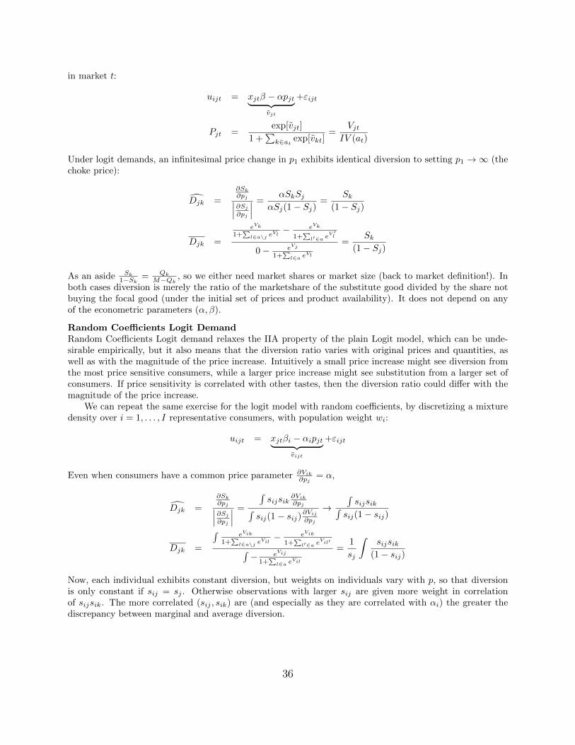
in market t:

uijt = xjtβ − αpjt︸ ︷︷ ︸vjt

+εijt

Pjt =exp[vjt]

1 +∑

k∈atexp[vkt]

=Vjt

IV (at)

Under logit demands, an infinitesimal price change in p1 exhibits identical diversion to setting p1 →∞ (thechoke price):

Djk =

∂Sk

∂pj∣∣∣∂Sj

∂pj

∣∣∣ =αSkSj

αSj(1− Sj)=

Sk

(1− Sj)

Djk =

eVk

1+∑

l∈a\j eVl− eVk

1+∑

l′∈a eV′l

0− eVj

1+∑

l∈a eVl

=Sk

(1− Sj)

As an aside Sk

1−Sk= Qk

M−Qk, so we either need market shares or market size (back to market definition!). In

both cases diversion is merely the ratio of the marketshare of the substitute good divided by the share notbuying the focal good (under the initial set of prices and product availability). It does not depend on anyof the econometric parameters (α, β).

Random Coefficients Logit DemandRandom Coefficients Logit demand relaxes the IIA property of the plain Logit model, which can be unde-sirable empirically, but it also means that the diversion ratio varies with original prices and quantities, aswell as with the magnitude of the price increase. Intuitively a small price increase might see diversion fromthe most price sensitive consumers, while a larger price increase might see substitution from a larger set ofconsumers. If price sensitivity is correlated with other tastes, then the diversion ratio could differ with themagnitude of the price increase.

We can repeat the same exercise for the logit model with random coefficients, by discretizing a mixturedensity over i = 1, . . . , I representative consumers, with population weight wi:

uijt = xjtβi − αipjt︸ ︷︷ ︸vijt

+εijt

Even when consumers have a common price parameter ∂Vik

∂pj= α,

Djk =

∂Sk

∂pj∣∣∣∂Sj

∂pj

∣∣∣ =

∫sijsik

∂Vik

∂pj∫sij(1− sij)∂Vij

∂pj

→∫sijsik∫

sij(1− sij)

Djk =

∫eVik

1+∑

l∈a\j eVil− eVik

1+∑

l′∈a eVil′∫− eVij

1+∑

l∈a eVil

=1

sj

∫sijsik

(1− sij)

Now, each individual exhibits constant diversion, but weights on individuals vary with p, so that diversionis only constant if sij = sj . Otherwise observations with larger sij are given more weight in correlationof sijsik. The more correlated (sij , sik) are (and especially as they are correlated with αi) the greater thediscrepancy between marginal and average diversion.

36