
An (exhaustive?) overview of optimization methodsdutangc.free.fr/pub/optim/optim_overview.pdf · 2...
25
An (exhaustive?) overview of optimization methods C. Dutang Summer 2010 1
Transcript of An (exhaustive?) overview of optimization methodsdutangc.free.fr/pub/optim/optim_overview.pdf · 2...

An (exhaustive?) overview of optimization methods
C. Dutang
Summer 2010
1

2 CONTENTS
Contents
1 Minimisation problems 3
1.1 Continuous optimisation, uncountable set X . . . . . . . . . . . . . . . . . . . . . . . . . . . . . . . . . . . . . . . . . . . 3
1.1.1 Unconstrained optimisation . . . . . . . . . . . . . . . . . . . . . . . . . . . . . . . . . . . . . . . . . . . . . . . . 3
1.1.2 Constrained optimisation . . . . . . . . . . . . . . . . . . . . . . . . . . . . . . . . . . . . . . . . . . . . . . . . . 8
1.1.3 Saddle point . . . . . . . . . . . . . . . . . . . . . . . . . . . . . . . . . . . . . . . . . . . . . . . . . . . . . . . . 11
2 Root problems 13
2.1 General equation, uncountable set X . . . . . . . . . . . . . . . . . . . . . . . . . . . . . . . . . . . . . . . . . . . . . . . 13
3 Fixed-point problems 17
4 Variational Inequality and Complementarity problems 18
4.1 Examples and problem reformulation . . . . . . . . . . . . . . . . . . . . . . . . . . . . . . . . . . . . . . . . . . . . . . . 18
4.1.1 Examples . . . . . . . . . . . . . . . . . . . . . . . . . . . . . . . . . . . . . . . . . . . . . . . . . . . . . . . . . . 18
4.1.2 Problem reformulation . . . . . . . . . . . . . . . . . . . . . . . . . . . . . . . . . . . . . . . . . . . . . . . . . . . 19
4.2 Algorithms for CPs . . . . . . . . . . . . . . . . . . . . . . . . . . . . . . . . . . . . . . . . . . . . . . . . . . . . . . . . . 20
4.3 Algorithms for VIPs . . . . . . . . . . . . . . . . . . . . . . . . . . . . . . . . . . . . . . . . . . . . . . . . . . . . . . . . 23
A Bibliography 24
B Websites 25

3
The following materials come mainly from Raydan & Svaiter (2001), Fletcher (2001), Madsen et al. (2004), Bonnans et al. (2006),Boggs & Tolle (1996), Dennis & Schnabel (1996), Conte & de Boor (1980), Ye (1996), Lange (1994) for optimization and root problems,Varadhan (2004), Roland et al. (2007) for fixed-point problems, and Facchinei & Pang (2003a,b) for variational inequality problems.
1 Minimisation problems
Minimisation problems consist in solving
minx∈X⊂Rn
f(x) such that cj(x) = 0, j ∈ E and cj(x) ≤ 0, j ∈ I.
Notations:– gradient vector g(x) = ∇f(x),– Hessian matrix H(x) = ∇2f(x),– Jacobian matrix of the function c Jc =
(∂ci∂xj
)ij
,
– positive and negative part of z, z+ = max(z, 0) and z− = −min(z, 0),– c(x)] is such that c(x)]i = ci(x) if i ∈ E or ci(x)+ if i ∈ I,– the superscript T denotes the transpose.
1.1 Continuous optimisation, uncountable set X
1.1.1 Unconstrained optimisation, E, I = ∅
1. Quadratic problems f(x) = 12x
TMx+ bTx+ c.Prop: unique solution if matrix M is symmetric positive and definite. Thus solve Mx+ b = 0.
(a) General descent scheme (xk+1 = xk + tkdk with stepsize tk and direction dk such that f(xk+1) < f(xk))
i. dk = −(Mxk + b): steepest descent method,
ii. dk = −(Mxk + b) and tk = (xk−xk−1)T (xk−xk−1)(xk−xk−1)TM(xk−xk−1)
: Barzilai-Borwein method,
iii. relaxed descent scheme (xk+1 = xk + tkθkdk with relaxation parameters 0 < θk < 2)
Assuming direction dk = −g(xk) and optimal stepsize tk = g(xk)T g(xk)g(xk)TMg(xk)
, the choice of relaxation parameters are– θk = 1 steepest descent method,– θk = 2 we get f(xk+1) = f(xk),– If the sequence (θk)k has an accumulation point θ? then the relaxed Cauchy method converges.

4 1 MINIMISATION PROBLEMS
(b) Conjugate gradient methods (xk+1 = xk + tkdk+1 given the full information at kth iteration):
i. classic CG method:– Init: x0, d1 = −g1
– Iter:gk+1 = gk + tkMdk with tk = − |gk|2
gTk Mdk
,
dk+1 = −gk+1 + ckdk with ck = |gk|2gT
k Mdk.
NB: all directions (d1, . . . , dk) are conjugate w.r.t. M .
ii. preconditioned conjugate gradient method,
(c) Gauss-Newton method for least square problems (f(x) =∑p
j=1 f2j (x))
Iteration is xk+1 = xk + dk with– dk = −G(xk)−1∇f(x),– gradient ∇f(x) =
∑pj=1 fj(x)∇fj(x),
– approximate Hessian G(x) =∑p
j=1∇fj(x)∇fj(x)T .
2. Smooth non linear problems f ∈ C1
(a) General descent scheme (xk+1 = xk + tkdk with stepsize tk and direction dk such that f(xk+1) < f(xk))Direction rule:
i. dk = arg min||d||<δ
g(xk)Td
– L1 norm, dk is the index of the largest component. Gauss Siedel?– L1 norm, dk = −g(xk): Steepest descent method.
Stepsize rule:
i. fixed: method of successive approximation,
ii. optimal tk = arg mint>0
f(xk + tdk) (useless in practice),
iii. Wolfe’s rule,
iv. Goldstein and Price,
v. Armijo.
Direction+Stepsize rule:
i. dk = −g(xk) and tk =dT
k−1dk−1
dTk−1(g(xk)−g(xk−1))
Barzilai-Borwein method,
ii. dk = −g(xk) and tk = arg mint>0
f(xk + tdk) Cauchy method,
(b) Conjugate gradient methods:

1.1 Continuous optimisation, uncountable set X 5
i. classic CG– Init: d1 = −g(x1)– Iter: dk = −g(xk) + βkdk−1 for k > 1
– βk = g(xk)T g(xk)g(xk−1)T g(xk−1)
: Fletcher-Reeves update,
– βk = g(xk)T (g(xk)−g(xk−1))g(xk−1)T g(xk−1)
: Polak-Ribiere update,– Beale-Sorenson,– Hestenses-Stiefel,– Conjugate-Descent,– . . .
NB: all directions (d1, . . . , dk) are conjugate to the Hessian matrix H(xk)?
ii. preconditionned CG
(c) Newton method (xk+1 = xk +dk with direction dk minimizes the quadratic function qf (d) = f(xk)+g(xk)Td+ 12d
T∇g(xk)d).
i. exact Newton method, dk solves g(xk) +∇g(xk)d = 0 i.e. minimizer of the local quadratic approximation qf .
ii. Quasi-Newton methods, dk approximates the exact minimizer of qfScheme:– Init: x0,W0
– Iter: while |g(xk)| > εapproximate Hessian inverse Wk = Wk−1 +Bkcompute direction dk = −Wkg(xk)line search for tk
Choice of W :– Constraints: symmetric, positive, definite and verified the quasi-Newton equation Wk(gk+1 − gk) = xk+1 − xk,– known methods for W : Davidon-Fletcher-Powell (DFP) or Broyden-Fletcher-Goldfarb-Shanno (BFGS).
iii. inexact Newton or truncated Newton methods:It requires that dk decreases the linear residual, ||H(xk)dk + g(xk)|| ≤ ηc||g(xk)||, where 0 < ηc < 1 is the forcing term.
NB: univariate case (n = 1), quasi-Newton has a unique equation: secant method or regula falsi method.
(d) Trust region algorithms (xk+1 = xk + hk with hk a local minimizer)Scheme:– hk(∆k) = arg min
||h||<∆k
f(xk) + g(xk)Th+ 12h
T Hkh with Hk is positive definite matrix,
– if f(xk + hk(∆k)) ≤ f(xk)−mhk(∆k) then terminates iteration,– otherwise decrease ∆k.NB: 0 < m < 1 a fixed coefficient.Choice of matrix Hk:

6 1 MINIMISATION PROBLEMS
– Hk is the Hessian H(xk): positive-definiteness is not guaranteed,– Hk = H(xk) + λIn with λ > 0: Levenberg-Marquardt algorithm (derived with KKT conditions),– quasi-Newton approximation,– Gauss-Newton approximationNB: Hk = 0 gives the steepest descent.
3. Non smooth problems
(a) direct search (derivative free) methods
i. Nelder-Mead algorithm
ii. Hooke-Jeeves algorithm
iii. multi-directional algorithm
iv. . . .
(b) metaheuristics
i. evolutionary algorithms
ii. stochastic algorithms– simulated annealing– Monte-Carlo method– ant colony
(c) regularizing techniques
i. filter algorithms
ii. noisy algorithms
(d) NSO methods
i. subgradient methods
ii. bundle methods
iii. gradient sampling methods
iv. hybrid methods
(e) special problems
i. piecewise linear
ii. minmax
iii. partially separable
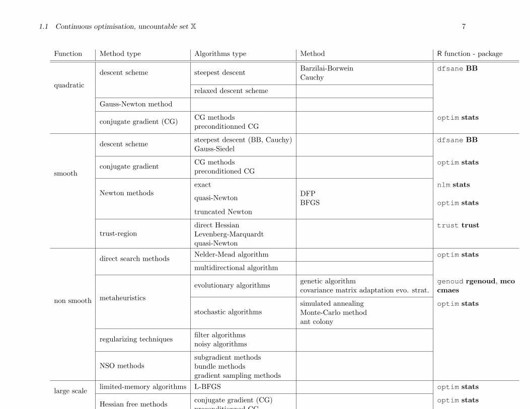
1.1 Continuous optimisation, uncountable set X 7
Function Method type Algorithms type Method R function - package
quadratic
descent scheme steepest descent Barzilai-Borwein dfsane BBCauchy
relaxed descent scheme
Gauss-Newton method
conjugate gradient (CG) CG methods optim statspreconditionned CG
smooth
descent scheme steepest descent (BB, Cauchy) dfsane BBGauss-Siedel
conjugate gradient CG methods optim statspreconditioned CG
Newton methodsexact nlm stats
quasi-Newton DFPBFGS optim stats
truncated Newton
trust-regiondirect Hessian trust trustLevenberg-Marquardtquasi-Newton
non smooth
direct search methods Nelder-Mead algorithm optim stats
multidirectional algorithm
metaheuristics
evolutionary algorithms genetic algorithm genoud rgenoud, mcocovariance matrix adaptation evo. strat. cmaes
stochastic algorithmssimulated annealing optim statsMonte-Carlo methodant colony
regularizing techniques filter algorithmsnoisy algorithms
NSO methodssubgradient methodsbundle methodsgradient sampling methods
large scale limited-memory algorithms L-BFGS optim stats
Hessian free methods conjugate gradient (CG) optim statspreconditionned CG

8 1 MINIMISATION PROBLEMS
1.1.2 Constrained optimisation (E, I 6= ∅), also known as nonlinear programming
The Lagrangian function is defined asL(x, λ) = f(x) + λT c(x),
with λ the Lagrange multiplier. The Karush-Kuhn-Tucker (KKT) conditions ∗ are– ∇xL(x, λ) = 0,– equality constraints ∀j ∈ E, cj(x) = 0 and λj ∈ R,– active inequality constraints j ∈ I, cj(x) = 0 and λj > 0,– inactive inequality constraints j ∈ I, cj(x) < 0 and λj = 0.
1. box constraints
(a) projected Newton method,
(b) limited-memory box-constraint BFGS method: L-BFGS-B,
2. linear constraints
(a) linear programming (f is linear)
i. simplex method,
ii. dual simplex method,
iii. Karmarkar algorithm,
(b) Interior point methods for linear constraintsConsider the problem min
xf(x) such that Ax = b and x ≥ 0. Let a log potential be π(x) = −
∑i log(xi). We want
to minimize the penalised function f(x) + µπ(x). A central path or path following algorithm is a sequence of points(x?µn
, λ?µn, s?µn
) solution of the problemx.s = µn11∇f(x) +ATλ = sAx = b
such that x ≥ 0, s ≥ 0,
for a sequence of decreasing (µn)n to 0.Main algorithms are
i. potential reduction algorithm,
ii. primal-dual symmetric algorithm,
∗. first order optimality conditions

1.1 Continuous optimisation, uncountable set X 9
iii. generic predictor-corrector algorithms or adaptive path-following algorithm,Generic predictor-corrector algorithms solve a linear complementarity reformulation of this problem with an iterativemethod:– a small-neighborhood algorithm,– a predictor-corrector algorithm with modified field,– a large-neighborhood algorithm.
3. general constraints
(a) Sequential linear programminglinearize both objective and constraint functions using Taylor series expansion.
(b) Sequential quadratic programming
i. Local methods for equality constraintsKKT conditions reduce to ∇f(x) + Jc(x)Tλ = 0 and c(x) = 0:– Newton method is an iterative method{
xk+1 = xk + dkλk+1 = λk + µk
computed from(∇2xxL(xk, λk) Jc(xk)T
Jc(xk) 0
)(dk
λk + µk
)= −
(∇f(xk)c(xk)
)– full Hessian approximation: replace ∇2
xxL with an approximated Hessian Bk (possible scheme PSB, BFGS),– augmented Lagrangian (add a constraint-penalty term) to guarantee positiveness,– reduced Hessian matrix: positiveness is only guaranteed on a subspace,
ii. Local methods for (in)equality constraintsThe SQP algorithm consists in solving a sequence of quadratic (Taylor) approximations of the Lagrangian.Scheme:– Init: x0, λ0
– Iterate while a termination criterionxk+1 = xk + dksolution of min
d∇f(xk)Td+ 1
2dT∇2
xxL(xk, λk)d
such that cE(xk) + JcE (xk)d = 0 and cI(xk) + JcI (xk)d ≤ 0Implementations:– active-set strategies,– interior-point algorithms,– dual approaches.
iii. Globalization of SQP methodA. trust region method:
Iterative method of a sequence of quadratic bounded sub-problem min||d||<∆k
∇f(xk)Td + 12d
TBkd, where the trust
region radius ∆k is updated at each stage.

10 1 MINIMISATION PROBLEMS
B. line search method:
Iterative method xk+1 = xk + tkdk, where direction dk is approximated by a solution of quadratic sub-problem andtk chosen to ensure a reasonable decrease of a merit function (e.g. f(x) + σ||c(x)]||p). NB: the penalty parameterhas to be updated (σk)k.
NB: for both those techniques, one particular approximation of the Hessian has to be chosen: quasi-Newton, reducedquasi-Newton, . . .
(c) Sequential unconstrained methods
i. Exterior point methods
The general idea is to minimize the merit function f(x) + p(x) where p is a. During the optimization process, anextertior-point method does not guarantee that all points are in the feasible region (hence the name).
Possible penalty terms are:
– quadratic penalty: p(x) = σ/2||c(x)]||22,– Lagrangian: p(x) = µT c(x),– augmented Lagrangian: p(x) = µT c(x) + σ/2||c(x)||22 with c(x)j = cj(x) if j ∈ E and max(−µj
σ , cj(x)) if j ∈ I,– non differentiable (exact) function: p(x) = σ||c(x)]||pThen we can either minimize of the associated Lagrangian function is carried out by an iterative method, or solve thedual problem arg max
u≥0θ(u) with θ(u) = min
xf(x) + up(x).
ii. Interior point methods (or adaptive barrier methods):
Barrier methods operates in the interior of the feasible region: adapting iteratively the barrier permits the convergenceto a boundary by lowering the strength of the corresponding barrier.
Let a log potential be π(x) = −∑
i log(xi). Using the convex property on f(x) + µπ(x), two majorants of f(x) can befound
– log surogate function: gl(x, y, µ) = f(x)− µ∑
j∈I cj(y) log cj(x) + µ∑
j∈I c′j(y)(x− y),
– power surogate function: gp(x, y, µ) = f(x) + µ∑
j∈I cj(y)α+β log cj(x)−α + µ∑
j∈I cj(y)βc′j(y)(x− y).
Then a MM algorithm can be used with an adaptive barrier constant µk:
– Init: x0, µ0,– Iterate while a termination criterionxk+1 = arg min
xgl(x, xk, µk) or arg min
xgp(x, xk, µk),
adapt µk+1.

1.1 Continuous optimisation, uncountable set X 11
Constraint type Method type Algorithm type Algorithms R function - package
box constraints projected Newton method
L-BFGS-B optim stats, Rvmmin
linear constraints
linear programsimplex method
dual simplex method
Karmarkar algorithm
interior-point methods
potential reduction algorithm
primal-dual symmetric algorithm
adaptive path-following algorithmsmall-neighborhood algorithm
predictor-corrector algorithm
large-neighborhood algorithm
general constraints
sequential linear program
sequential quadratic program trust-region SQP
line-search SQP
unconstrained program exterior-point algorithms
interior-point algorithms
1.1.3 Min-max saddle point
A saddle point x? satisfies the following inequality
∀u, v, φ(u?, v) ≤ φ(u?, v?) ≤ φ(u, v?),
with x = (uT vT )T . Grantham (2005) provide an unified way of most algorithms solving saddle points. If we see the iterative algorithmas a function of time, then iterative algorithm can be defined as the solution of partial differential equation (PDE). Let g be the
gradient of φ: g(x) = ∂φ∂x (x) =
(gu(x)gv(x)
). Then a general algorithm solve the PDE
∂x
∂t= −P (x)g(x),

12 1 MINIMISATION PROBLEMS
where P (x) denotes a matrix. Let H(x) be the Hessian matrix
H(x) =(Huu Huv
HTuv Hvv
)(x).
We have the following algorithms
1. steepest descent P (x) = diag(Iu,−Iv),2. Newton method P (x) = −H(x)−1,
3. gradient enhanced min-max
P (x) =(Huu + αuIu Huv
HTuv Hvv − αvIv
)(x)−1.

13
2 Root problems
Root problems consist in solvingf(x) = 0, x ∈ X ⊂ Rn.
2.1 General equation, uncountable set X
1. f linear: Ax = b
The solution is unique if A is invertible, i.e. det(A) 6= 0.
(a) direct inversionCompute A−1, then x = A−1b.
(b) Gaussian eliminationIf A is not upper triangular, transform A into a upper triangular matrix, and then compute ascendently the solution (if itexists). Note that it corresponds to a factorization PLU where L is a lower triangular matrix, U upper triangular and Ppermutation matrix.
i. Gauss pivot method
ii. Gauss Jordan method
iii. Grassman algorithm
(c) DecompositionDecompose A into three matrix D−E −F , with D the diagonal part, E the opposite lower part and F the opposite upperpart.
i. Jacobi iterations: xk+1 = D−1(E + F )xk +D−1b,
ii. Gauss-Siedel iterations: xk+1 = (D − E)−1Fxk + (D − E)−1b,
iii. Successive Over Relaxation: (D − ωE)xk+1 = (ωF + (1− ω)D)xk + ωb for ω ∈ [0, 1].
(d) projection methods for large scale problems
2. f univariate
(a) Newton methods
i. Newton-Raphson methodAssuming, we have the gradient f ′, the algorithm is– Init: x0
– Iter: xk+1 root of f(xk) + f ′(xk)(xk+1 − xk) = 0.

14 2 ROOT PROBLEMS
ii. the secant methodit consists in replacing f ′(xk) by a finite-difference approximation f(xk)−f(xk−1)
xk−xk−1in the Newton-Raphson method.
iii. the Muller methodIt consists in approximating the function by the quadratic function
q(x) = f(xk) + (x− xk)f [xk, xk−1] + (x− xk)(x− xk−1)f [xk, xk−1, xk−2],
where f [., .] denotes divided differences. Of course, analytical solution exists to find the next iterate xk+1.
(b) dichotomic search
i. bisection methodAssuming f is continuous, the procedure is– Init: a0 and b0 such that f(a0)f(b0) < 0,– Iter: let c = ak+bk
2 .If f(c)f(ak) > 0 then ak+1 = c, bk+1 = bk,otherwise bk+1 = c, ak+1 = ak.
ii. regula falsi or false position methoda hybrid combining dichotomic search and the secant method. Replace the c of the bissection method (middle of [ak, bk])by ck root of f(bk) + f(bk)−f(ak)
bk−ak(ck − bk) = 0.
3. f polynomial p
(a) Bairstow method:Consider a polynom with real coefficients. It consists in dividing succesively the polynom by a quadratic polynom. Thuswe get pairs of conjugate zeros.
(b) Bernoulli method:Iterative method that use the characteristic polynom to compute zero one after another, and deflate the polynom at eachstage.
(c) Muller method:Use a quadratic approximation of the polynom to find zeros.
(d) Newton method:Iterates the Newton method on the polynom. If combines with Muller method, it can be powerful to find zeros succesively.
(e) Laguerre method:It use the derivatives of log p, used in an iterative method.
(f) Durand-Kerner or Weierstrass method:Use a fixed-point iteration procedure to compute all roots at a time.
4. f smooth

2.1 General equation, uncountable set X 15
(a) Newton-Raphson method
Assuming, we have the gradient ∇f , the algorithm is
– Init: x0
– Iter: xk+1 root of f(xk) +∇f(xk)(xk+1 − xk) = 0.
(b) quasi-Newton methods
Approximate the gradient by Gk with an update scheme:
– Init: x0
– Iter: xk+1 root of f(xk) +Gk(xk+1 − xk) = 0.
Update schemes
– Broyden method : Gk = Gk−1 +(yk−1−Gk−1sk−1)sT
k−1
sTk−1sk−1
with yk−1 = f(xk)− f(xk−1) and sk = xk − xk−1.
– DFP or BFGS direct approximation of G−1k .

16 2 ROOT PROBLEMS
Function Methods Algorithms
linear
direct inversion
Gaussian eliminationGauss pivot methodGauss-Jordan methodGrassman method
decompositionJacobi iterationsGauss-Siedel iterationsSuccesive over relaxations
projection methods
univariateNewton method
Newton-Raphson methodsecant methodMuller method
dichotomic search bissection methodregula falsi
polynomial
BairstowBernoulliMullerNewtonLaguerreWeierstrass
smoothNewton-Raphson method
quasi-Newton BroydenBFGS
17
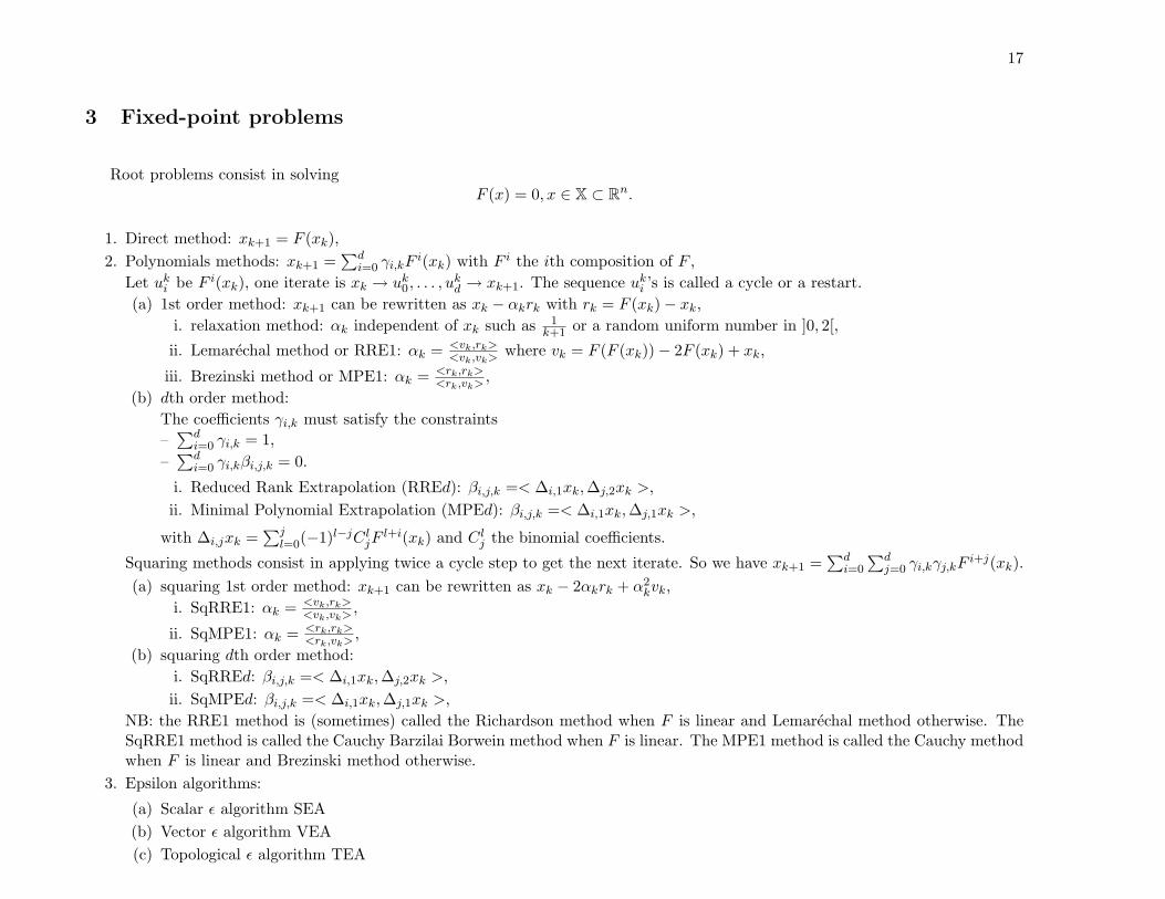
3 Fixed-point problems
Root problems consist in solvingF (x) = 0, x ∈ X ⊂ Rn.
1. Direct method: xk+1 = F (xk),2. Polynomials methods: xk+1 =
∑di=0 γi,kF
i(xk) with F i the ith composition of F ,Let uki be F i(xk), one iterate is xk → uk0, . . . , u
kd → xk+1. The sequence uki ’s is called a cycle or a restart.
(a) 1st order method: xk+1 can be rewritten as xk − αkrk with rk = F (xk)− xk,i. relaxation method: αk independent of xk such as 1
k+1 or a random uniform number in ]0, 2[,
ii. Lemarechal method or RRE1: αk = <vk,rk><vk,vk>
where vk = F (F (xk))− 2F (xk) + xk,
iii. Brezinski method or MPE1: αk = <rk,rk><rk,vk>
,(b) dth order method:
The coefficients γi,k must satisfy the constraints–∑d
i=0 γi,k = 1,–∑d
i=0 γi,kβi,j,k = 0.
i. Reduced Rank Extrapolation (RREd): βi,j,k =< ∆i,1xk,∆j,2xk >,ii. Minimal Polynomial Extrapolation (MPEd): βi,j,k =< ∆i,1xk,∆j,1xk >,
with ∆i,jxk =∑j
l=0(−1)l−jC ljFl+i(xk) and C lj the binomial coefficients.
Squaring methods consist in applying twice a cycle step to get the next iterate. So we have xk+1 =∑d
i=0
∑dj=0 γi,kγj,kF
i+j(xk).(a) squaring 1st order method: xk+1 can be rewritten as xk − 2αkrk + α2
kvk,i. SqRRE1: αk = <vk,rk>
<vk,vk>,
ii. SqMPE1: αk = <rk,rk><rk,vk>
,(b) squaring dth order method:
i. SqRREd: βi,j,k =< ∆i,1xk,∆j,2xk >,ii. SqMPEd: βi,j,k =< ∆i,1xk,∆j,1xk >,
NB: the RRE1 method is (sometimes) called the Richardson method when F is linear and Lemarechal method otherwise. TheSqRRE1 method is called the Cauchy Barzilai Borwein method when F is linear. The MPE1 method is called the Cauchy methodwhen F is linear and Brezinski method otherwise.
3. Epsilon algorithms:
(a) Scalar ε algorithm SEA(b) Vector ε algorithm VEA(c) Topological ε algorithm TEA

18 4 VARIATIONAL INEQUALITY AND COMPLEMENTARITY PROBLEMS
4 Variational Inequality and Complementarity problems
Variational inequality problems VI(K,F ) consist in finding x ∈ K such that
∀y ∈ K, (y − x)TF (x) ≥ 0,
where F : K 7→ Rn. We talk about quasi-variational inequality problems for the problem
∀y ∈ K(x), (y − x)TF (x) ≥ 0.
Complementarity problems CP(K,F ) consist in finding x ∈ K such that
x ∈ K,F (x) ∈ K?, xTF (x) = 0
where K? denotes the dual cone of K, i.e. K? = {d ∈ Rn,∀k ∈ K, kTd = 0}. Let us note xT y = 0 is equivalent to x is orthogonal toy, usually noted by x ⊥ y. Furthermore if K is a cone, then CP(K,F ) is equivalent to VI(K,F ).
4.1 Examples and problem reformulation
4.1.1 Examples
Here are few examples of VI problems.– classic complementary problems:
when K = Rn+, CP(K,F ) reduces to x ≥ 0 ⊥ F (x) ≥ 0, i.e. ∀i, xi ≥ 0, F (xi) ≥ 0, xiFi(x) = 0 ∗.
– mixed complementary problems:if K = Rm × Rm−n
+ and F (u, v) = (G(u, v)T , H(u, v)T )T , then G(u, v) = 0, v ≥ 0 ⊥ H(u, v) ≥ 0.– linear variational inequality problems:F (x) = q +Mx and K be a polyhedral set, a closed rectangle or the positive orthant.
– link with optimization problem:if we consider min
x∈Kθ(x) with K convex, then local minimizer must satisfy ∀y ∈ K, (y − x)T∇θ(x) ≥ 0, i.e. VI(K,∇θ). If
θ(x) = qTx+ 12x
TMx, then the VIP and the optimization are equivalent if M is symmetric and K is polyhedron.– extented KKT system:
Let K be {x ∈ Rn, h(x) = 0, g(x) ≤ 0} for h : Rn 7→ Rl and g : Rn 7→ Rm. If x solves VI(K,F ) then there exist µ ∈ Rl, λ ∈ Rm
such that
∗. Each composant of x and F (x) are complement.

4.1 Examples and problem reformulation 19
– L(x, µ, λ) = F (x) +∑
j µj∇hj(x) +∑
i λi∇gi(x) = 0,– h(x) = 0,– λ ≥ 0 ⊥ g(x) ≤ 0.
4.1.2 Problem reformulation
A necessary tool for VIP and CP is complementarity function. We say ψ : R2 7→ R is a complementarity function if ∀a, b ∈R2, ψ(a, b) = 0⇔ a ≥ 0, b ≥ 0, ab = 0. Here are some examples ψmin(x, y) = min(x, y), ψFB(x, y) =
√x2 + y2 − (x+ y).
A class of compl. function is the Mangasarian functions: ψMan(a, b) = ϕ(|a − b|) − ϕ(a) − ϕ(b) where ϕ is a strictly increasingfunction from R to R. Typically, we use ϕ(t) = t and ϕ(t) = t3.
Using this tool, we can reformulate the above extended KKT system as L(x, µ, λ)h(x)
ψmin(λ,−g(x))
= 0.
Another useful tool is the Euclidean projector on K, which for a point x find nearest on K according to the Euclidean distance.That is to say
ΠK : x 7→ arg miny∈K
12
(y − x)T (y − x).
There are two possibilities to reformulate VI(K,F ) problems:– natural mapping: x solves VI(K,F ) ⇔ FnatK (x) = 0 with FnatK (x) = x−ΠK(x− F (x)),– normal mapping: x solves VI(K,F ) ⇔ ∃z ∈ Rn, x = ΠK(z), FnorK (z) = 0 with FnorK (z) = F (ΠK(z)) + z −ΠK(z).
Example for CP(Rn+, F ), we have FnorK (z) = F (z+)− z−
The last tool we introduce is the merit functions. A merit function for VI(K,F ) is a function θ : X ⊂ K 7→ R+ such that x solvesVI(K,F ) ⇔ x ∈ X, θ(x) = 0⇔ x = arg min
y∈Xθ(y) for a closed set X and min
y∈Xθ(y) = 0.
Examples:– for VI(R+, F ) we have θψ(x) =
∑i ψ(xi, Fi(x))2 with ψ a compl. function,
– for VI(K,F ), we have θgap(x) = supy∈K
F (x)T (x− y). If K is a cone, then θgap(x) becomes xTF (x).
20 4 VARIATIONAL INEQUALITY AND COMPLEMENTARITY PROBLEMS
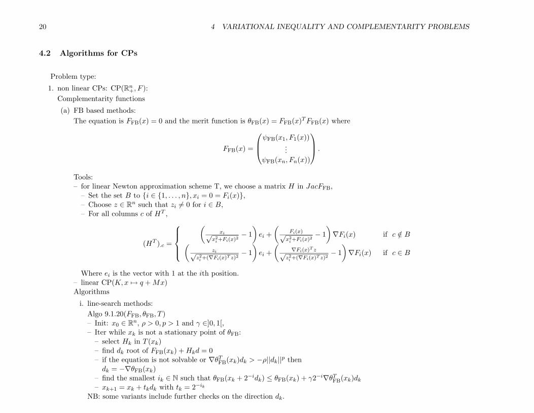
4.2 Algorithms for CPs
Problem type:
1. non linear CPs: CP(Rn+, F ):
Complementarity functions
(a) FB based methods:The equation is FFB(x) = 0 and the merit function is θFB(x) = FFB(x)TFFB(x) where
FFB(x) =
ψFB(x1, F1(x))...
ψFB(xn, Fn(x))
.
Tools:– for linear Newton approximation scheme T, we choose a matrix H in JacFFB,
– Set the set B to {i ∈ {1, . . . , n}, xi = 0 = Fi(x)},– Choose z ∈ Rn such that zi 6= 0 for i ∈ B,– For all columns c of HT ,
(HT ).c =
(
xi√x2
i +Fi(x)2− 1)ei +
(Fi(x)√x2
i +Fi(x)2− 1)∇Fi(x) if c /∈ B(
zi√z2i +(∇Fi(x)T z)2
− 1)ei +
(∇Fi(x)T z√
z2i +(∇Fi(x)T z)2− 1)∇Fi(x) if c ∈ B
Where ei is the vector with 1 at the ith position.– linear CP(K,x 7→ q +Mx)Algorithms
i. line-search methods:Algo 9.1.20(FFB, θFB, T )– Init: x0 ∈ Rn, ρ > 0, p > 1 and γ ∈]0, 1[,– Iter while xk is not a stationary point of θFB:
– select Hk in T (xk)– find dk root of FFB(xk) +Hkd = 0– if the equation is not solvable or ∇θTFB(xk)dk > −ρ||dk||p thendk = −∇θFB(xk)
– find the smallest ik ∈ N such that θFB(xk + 2−idk) ≤ θFB(xk) + γ2−i∇θTFB(xk)dk– xk+1 = xk + tkdk with tk = 2−ik
NB: some variants include further checks on the direction dk.

4.2 Algorithms for CPs 21
ii. trust region approachAlgo 9.1.35(FFB, θFB, T )– Init: x0 ∈ Rn, 0 < γ1 < γ2 < 1, ∆0,∆min > 0,– Iter:
– select Hk in T (xk)– find dk = arg min
||d||<∆k
qFB(d, xk) with qFB(d, x) = ∇θTFB(x)d+ 12d
THTk Hkd
– if qFB(dk, xk) = 0 then stops– if θFB(xk + dk) ≤ θFB(xk) + γ1qFB(dk, xk) then
xk+1 = xk + dk and ∆k ={
max(2∆k,∆min) if θFB(xk + dk) ≤ θFB(xk) + γ2qFB(dk, xk)max(∆k,∆min) otherwise
else xk+1 = xk and ∆k = ∆k/2NB: a variant includes an additional constraint on the direction dk.
iii. constrained methodsAlgo 9.1.39(FFB, θFB)– Init: x0 ∈ Rn, ρ > 0, p > 1 and γ ∈]0, 1[– Iter while xk is not a stationary point of θFB:
– find yk+1 solution of linear CP(qk, JacF (xk)) and dk = yk+1 − xk with qk = F (xk)− JacF (xk)xk,– if the equation is not solvable or ∇θTFB(xk)dk > −ρ||dk||p thendk = −min(xk,∇θFB(xk))
– find the smallest ik ∈ N such that θFB(xk + 2−idk) ≤ θFB(xk) + γ2−i∇θTFB(xk)dk– xk+1 = xk + tkdk with tk = 2−ik
NB: a variant consists in replacing the linear CP by a convex subprogram solved by a Levenberg-Marquardt method.
(b) min based methodsThe equation is Fmin(x) = 0 and the merit function is θmin(x) = Fmin(x)TFmin(x) where
Fmin(x) =
min(x1, F1(x))...
min(xn, Fn(x))
.
i. line-search methodIn the following, we use
φ(x, d) =∑
i,xi>Fi(x)
(Fi(x) +∇Fi(x)Td)2 +∑
i,xi≤Fi(x)
(xi + di)2 +ρ(θmin(x))
2dTd

22 4 VARIATIONAL INEQUALITY AND COMPLEMENTARITY PROBLEMS
andσ(x, d) =
∑i,xi>Fi(x)
Fi(x)∇Fi(x)Td+∑
i,xi≤Fi(x)
xidi.
Algorithm 9.2.2( Fmin, θmin, φ, σ)– Init: x0 ∈ Rn and γ ∈]0, 1[– Iter:
– find dk solution of arg minxk+d≥0
φ(xk, d)
– if dk = 0 then stops– find the smallest ik ∈ N such that θmin(xk + 2−idk) ≤ θmin(xk)− γ2−iσ(xk, dk)– xk+1 = xk + tkdk with tk = 2−ik
ii. trust region approachnot possible since min is not everywhere differentiable
iii. mixed compl. func. methodAlgorithm 9.2.3( FFB, θFB, Fmin)– Init: x0 ∈ Rn, ε > 0, p > 1, ρ > 0 and γ ∈]0, 1[– Iter while xk is not a stationary point of θFB:
– select Hk in Tmin(xk)– dk solves Fmin(xk) +Hkd = 0– if the system is solvable and ||Fmin(xk + dk)|| ≤ ||Fmin(xk)|| thenxk+1 = xk + tkdk with tk = 1
– else– if ∇θTFB(xk)dk > −ρ||dk||p thendk = −∇θFB(xk)
– find the smallest ik ∈ N such that θFB(xk + 2−idk) ≤ θFB(xk) + γ2−i∇θTFB(xk)dk– xk+1 = xk + tkdk with tk = 2−ik
(c) extension to other compl. functionsFB based methods can use with other complementarity functions. Here are some examples.– ψLT(a, b) = ||(a, b)||q − (a+ b) with q > 1
– ψKK(a, b) =√
(a−b)2+2qab−(a+b)
2−q with 0 ≤ q < 2– ψCCK(a, b) = ψFB(a, b)− qa+b+ with q ≥ 0.
2. finite lower VIs: CP(Rn+, F ):
3. finite upper VIs: CP(Rn+, F ):
4. mixed CPs
5. box constrained VIs

4.3 Algorithms for VIPs 23
4.3 Algorithms for VIPs

24 REFERENCES
A Bibliography
References
Boggs, P. T. & Tolle, J. W. (1996), ‘Sequential quadratic programming’, Acta Numerica . 3
Bonnans, J. F., Gilbert, J. C., Lemarechal, C. & Sagastizabal, C. A. (2006), Numerical Optimization: Theoretical and Practical Aspects,Second edition, Springer-Verlag. 3
Conte, S. D. & de Boor, C. (1980), Elementary numerical analysis: an algorithmic approach, Springer International series in pure andapplied mathematics. 3
Dennis, J. E. & Schnabel, R. B. (1996), Numerical methods for unconstrained optimization and nonlinear equations, SIAM. 3
Facchinei, F. & Pang, J.-S. (2003a), Finite-Dimensional Variational Inequalities and Complementary Problems. Volume I, Springer-Verlag New York, Inc. 3
Facchinei, F. & Pang, J.-S. (2003b), Finite-Dimensional Variational Inequalities and Complementary Problems. Volume II, Springer-Verlag New York, Inc. 3
Fletcher, R. (2001), ‘On the barzilai-borwein method’, Numerical Analysis Report 207. 3
Grantham, W. J. (2005), Gradient transformation trajectory following algorithms for determining stationary min-max saddle points.working paper. 11
Lange, K. (1994), Optimization, Springer-Verlag. 3
Madsen, K., Nielsen, H. B. & Tingleff, O. (2004), ‘Optimization with constraints’, Internet. 3
Raydan, M. & Svaiter, B. F. (2001), Relaxed steepest descent and cauchy-barzilai-borwein method. preprint. 3
Roland, C., Varadhan, R. & Frangakis, C. E. (2007), ‘Squared polynomial extrapolation methods with cycling: an application to thepositron emission tomography problem’, Numerical Algorithms 44(2), 159–172. 3
Varadhan, R. (2004), Squared extrapolation methods (squarem): a new class of simple and efficient numerical schemes for acceleratingthe convergence of the em algorithm. working paper. 3
Ye, Y. (1996), Interior-point algorithm: Theory and practice, online. 3

25
B Websites
– Applied mathematics: http://www.applied-mathematics.net,– Decision tree for optimization software: http://plato.asu.edu/guide.html,– Optimization online: http://www.optimization-online.org/cgi-bin/search.cgi,– Interior-point algorithms: http://www-user.tu-chemnitz.de/∼helmberg/sdp ip.html,