An Examination of Trip Generation and Travel Rate Indices for Alabama

Jointly Funded by The Alabama Department of Transportation and

The University Transportation Center for Alabama

By

Dr. Michael D. Anderson Department of Civil and Environmental Engineering

The University of Alabama in Huntsville Huntsville, Alabama 35899

Prepared by

UTCA

University Transportation Center for Alabama The University of Alabama, The University of Alabama in Birmingham, and

The University of Alabama at Huntsville

UTCA Report Number 01328 May 20, 2002

ii

Technical Report Documentation Page

1.Report No FHWA/CA/OR-

2.Government Accession No.

3.Recipient Catalog No.

4.Title and Subtitle An Examination Of Trip Generation And Travel Rate Indices For Alabama

5.Report Date May 20, 2002

7.Authors Michael Anderson

8. Performing Organization Report No. UTCA Report 01328 10.Work Unit No. 9.Performing Organization Name and Address

Civil and Environmental Engineering Department University of Alabama in Huntsville Huntsville, AL 35899 11.Contract or Grant No.

13.Type of Report and Period Covered Final Report/ 01/01/2001 – 04/30/2002

12.Sponsoring Agency Name and Address University Transportation Center for Alabama Box 870205, 271 H M Comer Mineral Industries Building Tuscaloosa, AL 35487-0205 14.Sponsoring Agency Code

15.Supplementary Notes

16.Abstract Transportation planning involves the decision-making process for potential improvements to a community’s roadway infrastructure. To aid in the decisions making process, several computer-based and manual tools have been developed. Two of these key tools are (1) travel demand forecasting models for implementing the four-step urban planning process, and (2) travel rate indices for providing congestion and delay information for a community. This report focuses on the trip generation step of the urban transportation planning process as well as the calculation of travel rate indices for the thirteen urban areas within Alabama. Among the major finding of this study of trip generation in Alabama was that several factors influence trip making behavior, not just income, however, the existing trip generation methodology employed by the Alabama communities is capable of accurately forecasting trip making behavior if updated properly to reflect current socio-economic conditions. 17.Key Words Travel forecasting, trip generation, travel rate indices

18.Distribution Statement

19.Security Class (of this report)

20.Security Class (of this page) 21.No. of pages 61

22.Price

iii

Contents

Contents…………………………………………………………………………………..... iii

Tables ……………………………………………………………………………………… iv

Figures …………………………………………………………………………………….. iv

Executive Summary……….……………………………………………………………….. v

1.0 Introduction……………………………………………………………………………. 1

2.0 Data Collection for Trip Distribution……………………………………………….…. 3

3.0 Recoding of the Trip Generation Software…………………………………………….. 7

4.0 Coding of an Alternate Trip Generation Software…………………………………….. 12

5.0 Travel Rate Indices for Alabama’s Urban Communities……………………………… 15

6.0 Analysis of Trip Generation in Alabama………………………………………………. 24

7.0 Conclusion …………………………………………………………………………….. 33

Appendix A: Trip Generation Software Technical Manual……………………………….. 35

Appendix B: Trip Generation Software Flowchart ……………………………………….. 46

iv

List of Tables

Number Page Table 2-1 Trip production values for the study communities…………………………. 6 Table 4-1 Production information from NCHRP 365…………………………………. 12 Table 5-1 Roadway categories………………………………………………………… 15 Table 5-2 Summary of the travel rate indices calculations……………………………. 23

List of Figures Number Page Fig 2-1 Zones studied in Birmingham………………………………………………. 4 Fig 2-1 Zones studied in Decatur…………………………………………………… 4 Fig 2-3 Zones studied in Huntsville………………………………………………… 5 Fig 3-1 Data entry screen from the existing software………………………………. 7 Fig 3-2 Output form the existing software showing the different trip purposes……. 8 Fig 3-3 Formatted output file from the existing software…………………………... 8 Fig 3-4 Input file for the program…………………………………………………… 9 Fig 3-5 Screen for finding necessary input files…………………………………….. 10 Fig 3-6 Summary of socio-economic data provided by the software………………. 10 Fig 3-7 Example of one screen used to update the internal parameters……………. 11 Fig 4-1 Start-up screen……………………………………………………………… 13 Fig 4-2 Summary of the trip generation run………………………………………… 14 Fig 4-3 Output form the software…………………………………………………… 14 Fig 5-1 Anniston, AL……………………………………………………………….. 17 Fig 5-2 Auburn, AL…………………………………………………………………. 17 Fig 5-3 Birmingham, AL……………………………………………………………. 18 Fig 5-4 Decatur, AL………………………………………………………………… 18 Fig 5-5 Dothan, AL…………………………………………………………………. 19 Fig 5-6 Gadsden, AL………………………………………………………………... 19 Fig 5-7 Huntsville, AL……………………………………………………………… 20 Fig 5-8 Mobile, AL…………………………………………………………………. 20 Fig 5-9 Montgomery, AL…………………………………………………………… 21 Fig 5-10 Opelika, AL………………………………………………………………… 21 Fig 5-11 Phoenix City, AL…………………………………………………………… 22 Fig 5-12 Shoals Area, AL…………………………………………………………….. 22 Fig 5-13 Tuscaloosa, AL……………………………………………………………... 23

v

Executive Summary Transportation planning involves the decision-making process for potential improvements to a community’s roadway infrastructure. To aid in the decisions making process, several computer-based and manual tools have been developed. Two of these key tools are (1) travel demand forecasting models for implementing the four-step urban planning process, and (2) travel rate indices for providing congestion and delay information for a community. This report focuses on the trip generation step of the urban transportation planning process as well as the calculation of travel rate indices for the thirteen urban areas within Alabama. There are five key tasks discussed in this report. First, a data collection study was performed by the University of Alabama in Huntsville to assess the trip generation rates within the urban communities of Alabama. The data collection efforts focused on Birmingham, Decatur, and Huntsville. Second, the existing QuickBasic software developed to perform trip generation within Alabama was rewritten in VisualBasic to provide a more user- friendly version of the software with improved updating capabilities. Third, a VisualBasic program was developed to implement the trip generation methodology of the National Cooperative Highway Research Program Report 365. The new program provides an alternative to the Alabama trip generation methodology. Fourth, travel rate indices and costs of congestion were calculated for the thirteen urban areas in the state. Finally, factors that contribute to trip generation behavior in Alabama were developed. This examination resulted from the data collected for Birmingham, Decatur, and Huntsville and information provided in the recently released census figures for these communities. The examination of factors also includes a comparison of Alabama’s trip generation methodology to a nationally recommended trip generation procedure.

The first task, data collection, was performed for three urban communities representing the three sizes of cities found in Alabama. The results of the data collection study were used to determine if the existing software was capable of explaining trip making characteristics within the urban areas. Results of this analysis proved that the existing software was capable of calculating trip productions tendencies, provided that the curves used in the software were updated on a regular basis, proposed to be approximately every five years. This conclusion reflects Birmingham’s recent data collection study and updating of its trip curves, whereas in Decatur and Huntsville the existing software curves were dated and were not able to provide an accurate determination of current trip production values. The second task, the recoding of the existing software into VisualBasic, was undertaken to make the program more user- friendly. As determined in the first task, the software has the ability to accurately calculate trip production rates, with updated curves. The VisualBasic implementation of the software hopefully provides a user- friendly interface for agencies to utilize during the trip generation step of the modeling process. It also provides several easy-to-understand screens that

vi

agencies can use to update their specific curves, making sure the software will be continuously capable of predicting trip making. The third task, coding of another trip generation model in VisualBasic, was performed as a method to determine the validity of the existing trip generation software model and to provide an alternative to communities within Alabama for performing trip generation. The method follows standard practices and is therefore presented as an alternative. The fourth task, the development of the travel rate indices, was presented as information for urban communities within Alabama as a metric to determine their level of congestion. The information calculated, including the travel rate index, cost of wasted fuel, and total cost of congestion, is intended to present a view of the existing roadway network and to serve as a baseline to determine optimum infrastructure decisions in the future. It is proposed that the methodology should be performed on a four to five year cycle, as a means to provide transportation planners within the urban communities some indication as to whether or not the decisions they are making are reducing the congestion within their communities. The fifth task was an analysis of the trip generation process for Alabama. It indicated that the existing trip generation software is reflective of the national trip generation procedure, and provided alternative regression equations (using different data sources) for performing trip generation within urban areas. One key conclusion from the analysis is that trip making is not a direct reflection of income for any of the communities studied. Others factors, such as median age of residents, distribution of ages of residents, and average household size have a larger influence of the number of trips made. This information is an important first step in the determination of a new trip generation model for Alabama, if one is so desired. Overall, this study of trip generation in Alabama concluded that several factors influence trip making behavior, not just income; however, the existing trip generation methodology employed by Alabama communities is capable of accurately forecasting trip making behavior if updated properly to reflect current socio-economic conditions.

1

Section 1 Introduction

Transportation planning involves the decision-making process for potential improvements to a community’s roadway infrastructure. To aid in the decision-making process, several computer-based and manual tools have been developed. Two of these key tools are (1) travel demand forecasting models for implementing the four-step urban planning process, and (2) travel rate indices for providing congestion and delay information for a community. The four-step urban planning process is comprised of the following: Trip Generation, Trip Distribution, Mode Split, and Traffic Assignment.

• Trip Generation uses mathematical models to determine the number of productions and attractions associated with each zone in the community

• Trip Distribution determines the allocation of trips between different zones in the community

• Mode Split identifies the number of trips that will use the various modes of transportation available within the community

• Traffic Assignment calculates the number of trips that are forecasted to use each of the different routes available.

Within Alabama, trip generation is performed using a QuickBasic program developed by the Alabama Department of Transportation. Trip distribution is performed using TRANPLAN, a popular commercial software package developed by the Urban Analysis Group that implements the travel demand forecasting process. Mode split is generally ignored in Alabama as the number of transportation alternatives is limited and transit usage represents a very small percentage of the total trips made. Traffic assignment is performed using TRANPLAN software. Travel rate indices were developed as part of an urban mobility study performed at Texas A&M University to assess congestion and delay. In the original study, several urban communities around the country were studied. However, the study did not include any Alabama communities. The calculation of these indices is performed using roadway traffic volumes and a series of tables and equations to determine the anticipated travel speed for the different roadways. These travel speeds are then used as a measure of the delay associated within the community. Travel indices calculations provide information regarding the amount of delay experienced within a community and cost estimates associated with that delay. This report focuses on the trip generation step of the urban transportation planning process, as well as the calculation of travel rate indices for the thirteen urban areas within Alabama. There are five key tasks discussed in this report. First, a data collection study was performed by the

2

University of Alabama in Huntsville to assess the trip generation rates within the urban communities of Alabama. The data collection efforts focused on Birmingham, Decatur, and Huntsville. Second, the existing QuickBasic software developed to perform trip generation within Alabama was rewritten in VisualBasic to provide a more user- friendly version with improved updating capabilities. Third, a VisualBasic program was developed to implement the trip generation methodology of National Cooperative Highway Research Program Report 365, presented as an alternative to the Alabama trip generation methodology. Fourth, calculations of the travel rate indices and costs of congestion in the thirteen urban areas in the state were provided. Finally, an examination was made of factors that contribute to trip generation behavior in Alabama. This examination concentrated on the data collected for Birmingham, Decatur, and Huntsville and on the information provided in the recently released census figures for these communities. The examination of factors also included a comparison of Alabama’s trip generation methodology to a nationally recommended trip generation procedure.

3

Section 2 Data Collection for Trip Generation

During the summer of 2001, students of the University of Alabama in Huntsville undertook an extensive data collection effort. The effort determined the number of trips made into and out of various zones in the community as well as the number of households in the zone that contributed to the traffic. Originally, the project was to collect a small sample of data from all of the urban areas within Alabama. However, members of the Alabama Transportation Planners Association suggested that better results would be obtained if three representative communities were selected and a more intensive data collection effort was performed in these areas. Within Alabama, three unique community sizes were identified, those around 50,000 (small), those between 75,000 and 200,000 (medium), and those greater than 250,000 (large). Members from the representative communities selected Decatur (similar to Anniston, Auburn, Dothan, Gadsden, Opelika, Phenix City, and the Shoals), Huntsville (similar to Mobile, Montgomery, and Tuscaloosa) and Birmingham (the only large city in Alabama). The selection of zones for the data collection effort was based on the ability to provide a variety of socio-economic characteristics as well as the ability to develop a captive group of households. By pre-screening the study zones and examining the census information, variety was ensured in the zones selected. Selection of locations within the zones where a large number of households were located with limited entry/exit points available ensured a captive population and made it possible for a limited number of student data collectors to cover a large zone. Figures 2-1, 2-2, and 2-3 show the locations of the zones studied for Birmingham, Decatur, and Huntsville.

4

Figure 2-1. Zones studied in Birmingham.

Figure 2-2. Zones studied in Decatur.

5

Figure 2-3. Zones studied in Huntsville. The data collected in the three communities consisted of trips into and out of each zone. These trip values were collected over a couple of hours of the day; they were then factored into daily trips using nationally published factors from the National Cooperative Highway Research Program Report 365. In addition, these trip rates were adjusted further based on the actual number of households from which the sample was collected and the actual number of households contained in the zone, as reported by the communities. These factored daily trips serve as actual trips made within the zone. The existing trip generation software was used to determine the projected number of productions and attractions that would be the calculated using the standard methodology. Table 2-1 shows the difference in values for the zones from the three study communities. A statistical analysis concluded that there was a significant difference between the actual trip production values collected and the production values calculated using the software for Decatur and Huntsville (at the 95% confidence level). For Birmingham, there was no significant difference between the production values developed by the data collection study and the trip generation software.

6

Table 2-1. Trip production values for the study communities Birmingham Decatur Huntsville Zone S/W Count Zone S/W Count Zone S/W Count 19 474 411 58 1285 2331 39 5754 7255 35 2299 3983 68 959 2511 50 2300 1985 39 3730 4876 78 677 661 60 1073 15994 151 1713 3857 86 1631 4758 64 2930 6252 290 6495 11084 111 3480 3865 69 3090 1110 169 1271 1451 128 8117 1176 82 5756 5991 211 473 203 150 1501 1467 89 3970 2488 258 14446 19187 156 4375 15592 100 16037 5555 274 1438 3732 169 530 724 113 1162 1193 381 2659 5136 206 1889 914 114 3271 45281 459 7366 7114 242 2345 2581 115 5365 58285 490 3673 15144 245 749 2001 153 1430 2257 497 3277 4538 252 3732 7185 173 243 291 575 8488 9864 264 3179 5211 197 1847 1234 576 6537 9406 265 3179 4899 214 315 1333 592 4243 2546 247 3100 2631 609 441 636 622 2040 5758 633 3329 2579 639 2499 2608

The evaluation of the trip generation software using the data collected in this research demonstrate that the existing program can be used to accurately determine the number of productions and attractions for a zone. This observation/conclusion was based on the analysis of Birmingham, where there was no statistical difference between the values predicted by the software and values obtained during our study. However, it is important to note that this result is probably due to a recent study undertaken by the Regional Council of Greater Birmingham to update internal parameters of their model. These improvements were not available to adjust the trip generation software parameters for Decatur and Huntsville. It is the conclusion of this work that the existing methodology is a viable approach if the appropriate measures are undertaken to ensure that community parameters are current.

7

Section 3 Recoding of the Trip Generation Software

The existing trip generation software program developed by the Alabama Department of Transportation is used to convert socio-economic data into production and attraction values, based on a series of “curves” which contain factors that include automobile ownership, trips per household, production and attraction factors, external trip factors, and income ranges. The existing program, written in QuickBasic, operates in a DOS window under the Windows operating system. The prompts for this program are all user entered and there is limited information provided by the program to assist the user in the operation of the program. Figures 3-1 and 3-2 show screens from the existing program.

Figure 3-1. Data entry screen from the existing software.

8

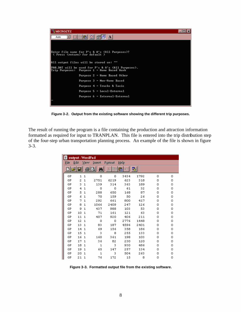
Figure 3-2. Output from the existing software showing the different trip purposes. The result of running the program is a file containing the production and attraction information formatted as required for input to TRANPLAN. This file is entered into the trip distribution step of the four-step urban transportation planning process. An example of the file is shown in figure 3-3.

Figure 3-3. Formatted output file from the existing software.

9

The recoded VisualBasic program was written to replicate the operation of the original QuickBasic program. The objective of the program remained constant even though the programming language changed, conversion of socio-economic data to production and attraction values for a community. Some of the key elements of the program include enhanced data entry screens, user assistance for data entry, and screens for modification of the internal parameters (a feature not available in the original program). To demonstrate the recoded program, figures 3-4, 3-5, 3-6, and 3-7 provide example screen shots.

Figure 3-4. Input file for the program.

10

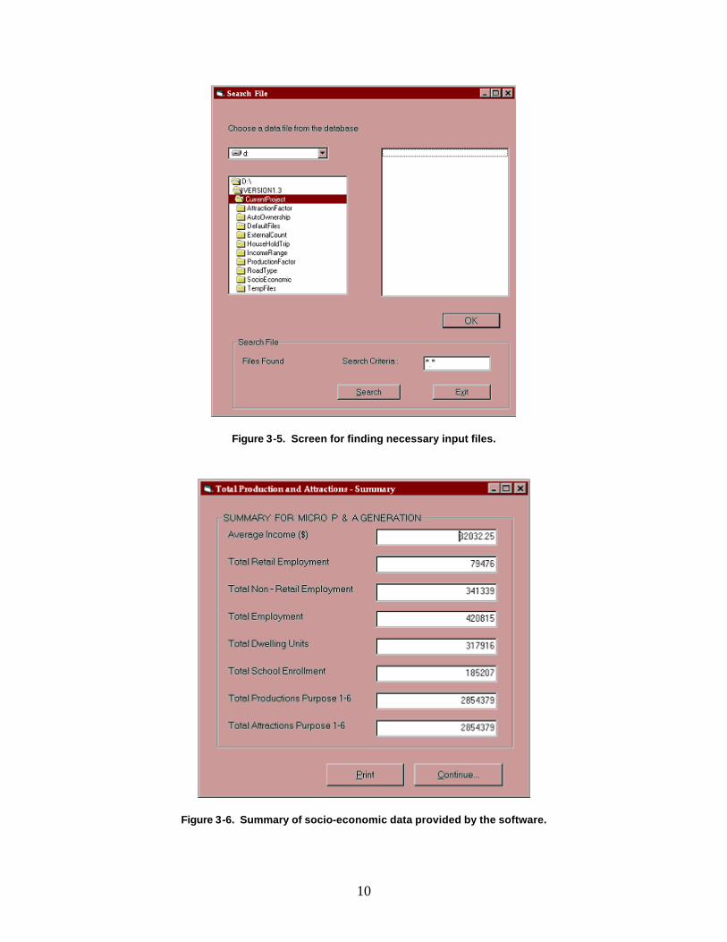
Figure 3-5. Screen for finding necessary input files.

Figure 3-6. Summary of socio-economic data provided by the software.

11

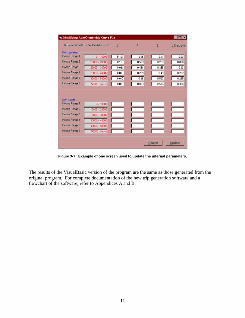
Figure 3-7. Example of one screen used to update the internal parameters. The results of the VisualBasic version of the program are the same as those generated from the original program. For complete documentation of the new trip generation software and a flowchart of the software, refer to Appendices A and B.

12

Section 4 Coding of an Alternate Trip Generation Program

The trip generation methodology used within Alabama, by no means represents the only methodology for performing trip generation. Another popular, national method was developed through the National Cooperative Highway Research Program (NCHRP). This methodology uses classification tables, similar to those used in the existing Alabama model, to calculate trip productions and regression equations to calculate trip attractions. The NCHRP procedure uses four different cross-classification tables for productions, based on the population of the community of interest. For Alabama, the three relevant tables are (NCHRP Report 365) shown below. Table 4-1. Production information from NCHRP 365 Urban Area = 50,000 – 199,999 % Average Daily Average Person Trips by Daily person Purpose Income Per Household HBW HBO NHB Low 6.7 16 60 24 Medium 10.0 21 56 23 High 12.8 20 55 25 Urban Area = 200,000 – 499,999 % Average Daily Average Person Trips by Daily person Purpose Income Per Household HBW HBO NHB Low 6.8 17 60 23 Medium 9.5 20 56 24 High 12.4 23 52 25 Urban Area = 500,000 – 999,999 % Average Daily Average Person Trips by Daily person Purpose Income Per Household HBW HBO NHB Low 6.6 18 59 23 Medium 8.8 23 55 22 High 11.6 22 54 24

The NCHRP procedure uses three different regression equations for attractions (NCHRP Report 365): HBW attractions = 1.45 * TE HBO attractions = 9.0 * RE + 1.7 * SE + 0.5 * OE + 0.9 * HH NHB attractions = 4.1 * RE + 1.2 * SE + 0.5 * OE + 0.5 * HH

13

Where: TE = Total Employment

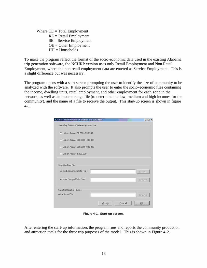
RE = Retail Employment SE = Service Employment OE = Other Employment HH = Households To make the program reflect the format of the socio-economic data used in the existing Alabama trip generation software, the NCHRP version uses only Retail Employment and Non-Retail Employment, where the non-retail employment data are entered as Service Employment. This is a slight difference but was necessary. The program opens with a start screen prompting the user to identify the size of community to be analyzed with the software. It also prompts the user to enter the socio-economic files containing the income, dwelling units, retail employment, and other employment for each zone in the network, as well as an income range file (to determine the low, medium and high incomes for the community), and the name of a file to receive the output. This start-up screen is shown in figure 4-1.

Figure 4-1. Start-up screen. After entering the start-up information, the program runs and reports the community production and attraction totals for the three trip purposes of the model. This is shown in Figure 4-2.

14

Figure 4-2. Summary of the trip generation run.

The result of running the program is a file containing the production and attraction information formatted as required by TRANPLAN. This file is entered into the trip distribution step of the four-step urban transportation planning process. An example of the file is shown in figure 4-3. The columns include the zone number, home based work productions, home based other productions, non-home based productions, home based work attractions, home based other attractions, and non-home based attractions.

Figure 4-3. Output from the software.

15

Section 5 Travel Rate Indices for Alabama’s Urban Communities

The trip generation indices calculation and results were developed following the methodology developed in the urban mobility study, originally performed by Texas A&M University. Within this section of the report, the methodology work steps and results are presented for the thirteen urban communities within the state. Special thanks are extended to the Alabama Department of Transportation for providing the traffic count information for the thirteen communities that allowed these calculations to be undertaken. The initial step of the methodology included data collection. For the study, roadway information and traffic count data were needed. The roadway data included the length of the roadway segment, the classification (arterial or freeway), and the number of lanes (taken to be 4 for an arterial and 6 for a freeway). The roadway data was collected and stored in a geographic information system (GIS) to ease in the data manipulation and update process. The Alabama Department of Transportation provided traffic counts for specific roadways within the thirteen urban areas. These counts and corresponding segment s of roadways where the traffic would remain relatively constant were digitized over the background roadway data, which was used for visual interpretation. The newly digitized roadway was updated, through database modifications, and attributed with the classification of the facility, the number of lanes, and the length of the facility (determined by the GIS program). Based on the traffic volume for the roadway, a table provided in the urban mobility study was used to classify each roadway into one of eight categories. Table 5-1. Roadway categories Arterial Freeway Moderate Congestion Moderate Congestion Heavy Congestion Heavy Congestion Severe Congestion Severe Congestion Extreme Congestion Extreme Congestion

Using the traffic count, length of the roadway, and classification for the facility, it was possible to determine the vehicle miles of travel (VMT) for the community for each roadway condition. Based on information from the urban mobility study, it was then possible to determine the operating speed for the facilities. This information was exported from the GIS to a spreadsheet program for the remainder of the analysis. Within the spreadsheet program, the VMT for each classification was determined through an aggregation process. The VMT were then adjusted by 45% to account for delay, as recommended by the Texas A&M study. Next, the recurring vehicle-hours of delay were

16

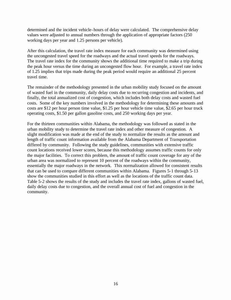
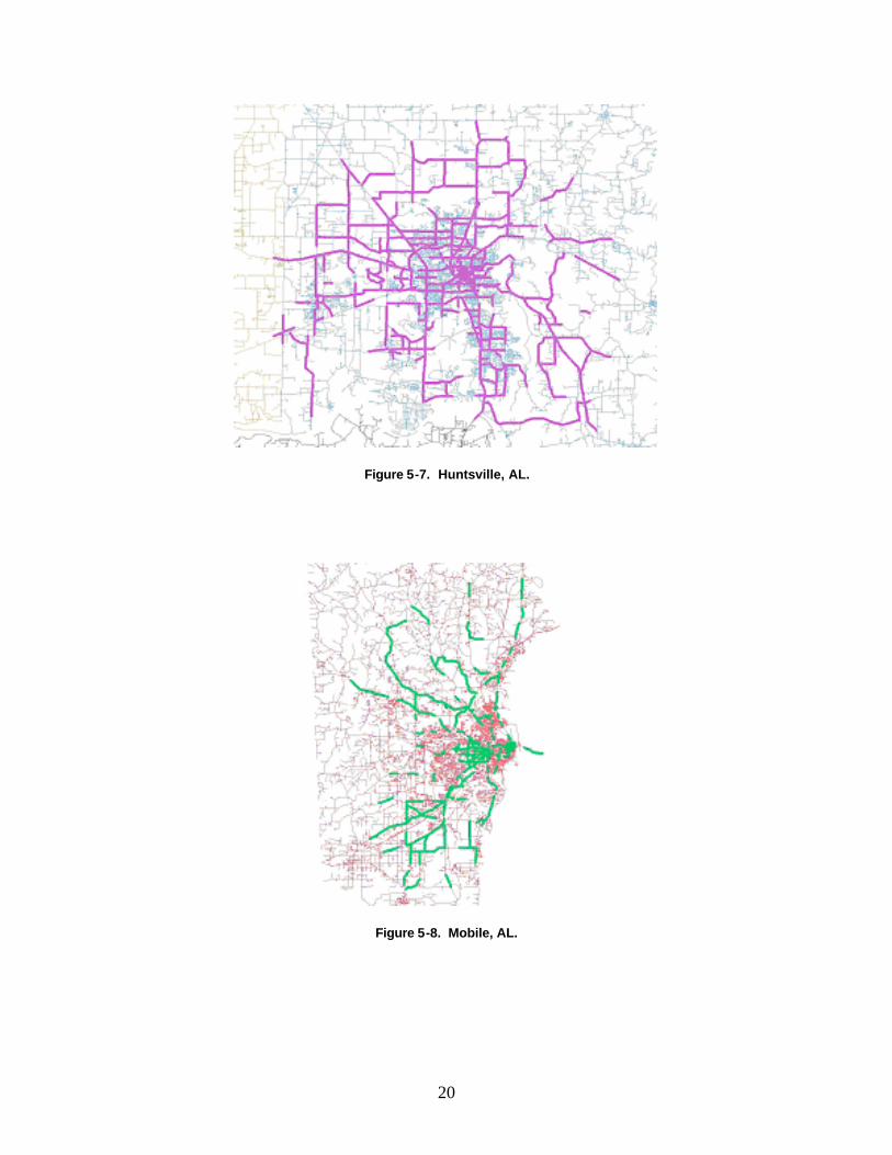
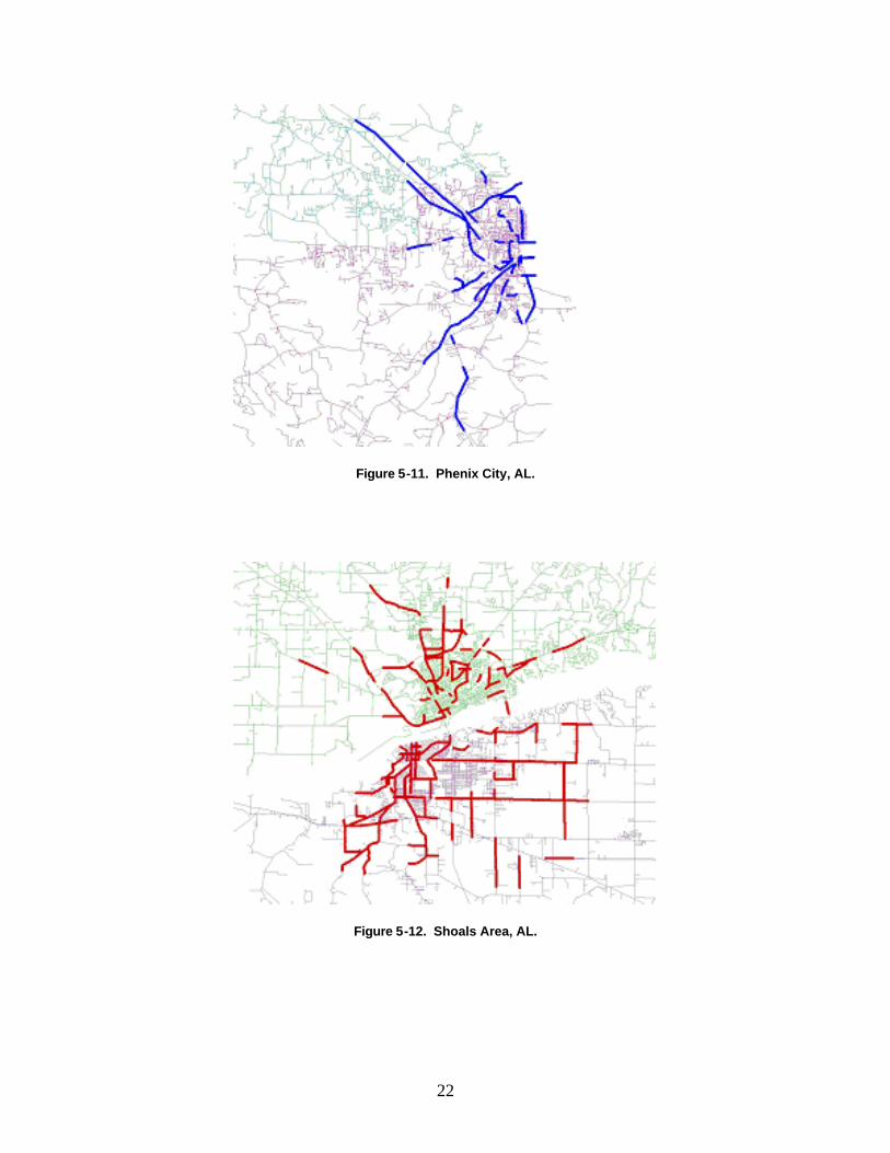
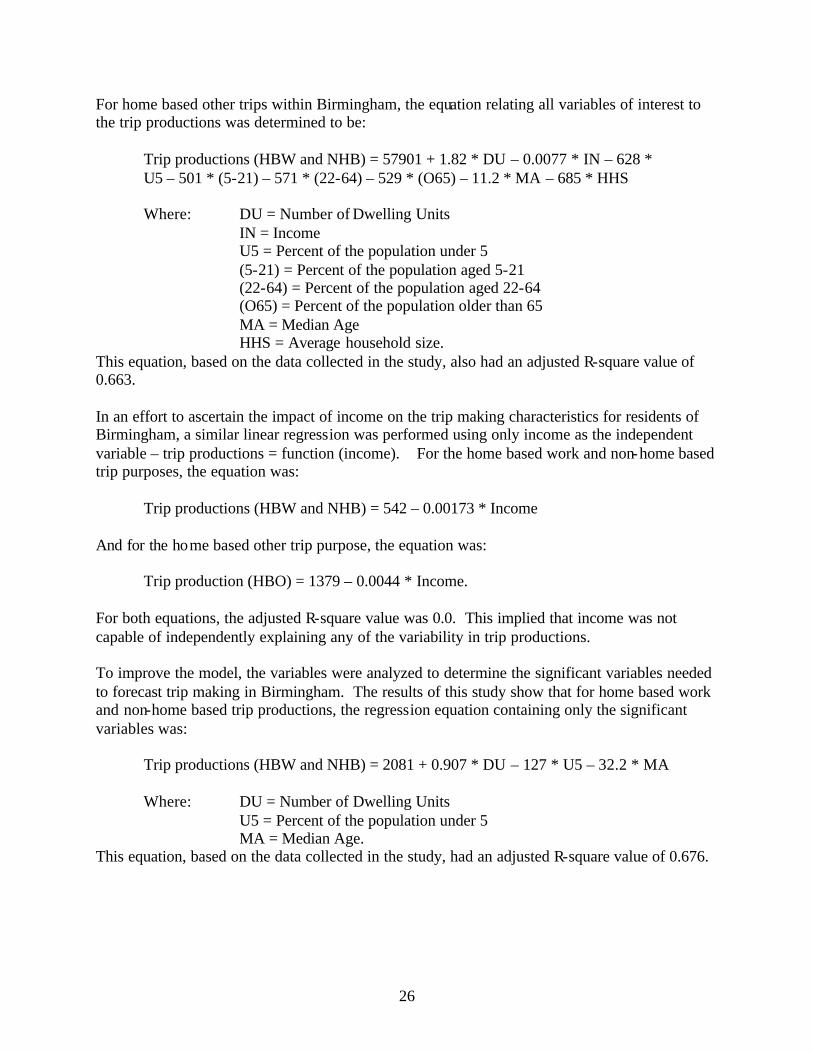
determined and the incident vehicle-hours of delay were calculated. The comprehensive delay values were adjusted to annual numbers through the application of appropriate factors (250 working days per year and 1.25 persons per vehicle). After this calculation, the travel rate index measure for each community was determined using the uncongested travel speed for the roadways and the actual travel speeds for the roadways. The travel rate index for the community shows the additional time required to make a trip during the peak hour versus the time during an uncongested flow hour. For example, a travel rate index of 1.25 implies that trips made during the peak period would require an additional 25 percent travel time. The remainder of the methodology presented in the urban mobility study focused on the amount of wasted fuel in the community, daily delay costs due to recurring congestion and incidents, and finally, the total annualized cost of congestion, which includes both delay costs and wasted fuel costs. Some of the key numbers involved in the methodology for determining these amounts and costs are $12 per hour person time value, $1.25 per hour vehicle time value, $2.65 per hour truck operating costs, $1.50 per gallon gasoline costs, and 250 working days per year. For the thirteen communities within Alabama, the methodology was followed as stated in the urban mobility study to determine the travel rate index and other measure of congestion. A slight modification was made at the end of the study to normalize the results as the amount and length of traffic count information available from the Alabama Department of Transportation differed by community. Following the study guidelines, communities with extensive traffic count locations received lower scores, because this methodology assumes traffic counts for only the major facilities. To correct this problem, the amount of traffic count coverage for any of the urban area was normalized to represent 10 percent of the roadways within the community, essentially the major roadways in the network. This normalization allowed for consistent results that can be used to compare different communities within Alabama. Figures 5-1 through 5-13 show the communities studied in this effort as well as the locations of the traffic count data. Table 5-2 shows the results of the study and includes the travel rate index, gallons of wasted fuel, daily delay costs due to congestion, and the overall annual cost of fuel and congestion in the community.

17

Figure 5-1. Anniston, AL.

Figure 5-2. Auburn, AL.

18

Figure 5-3. Birmingham, AL.

Figure 5-4. Decatur, AL.

19

Figure 5-5. Dothan, AL.

Figure 5-6. Gadsden, AL.

20

Figure 5-7. Huntsville, AL.

Figure 5-8. Mobile, AL.

21

Figure 5-9. Montgomery, AL.

Figure 5-10. Opelika, AL.

22

Figure 5-11. Phenix City, AL.

Figure 5-12. Shoals Area, AL.

23

Figure 5-13. Tuscaloosa, AL. Table 5-2. Summary of the travel rate index calculations Community Travel Rate Index Wasted Fuel (Gal) Total Delay Costs ($) Annual Delay Costs ($) Anniston 1.30 4,946,449 182,565 53,060,905 Auburn 1.29 1,177,086 43,592 6,582,100 Birmingham 1.39 33,534,398 1,300,863 375,517,256 Decatur 1.33 3,186,012 118,632 34,436,928 Dothan 1.28 2,055,519 75,339 21,918,044 Gadsden 1.33 6,762,709 252,218 73,198,557 Huntsville 1.36 11,177,383 421,011 63,633,185 Mobile 1.28 11,328,929 415,629 120,900,738 Montgomery 1.35 12,767,151 487,542 138,786,197 Opelika 1.21 468,046 16,966 4,943,604 Phenix City 1.28 1,278,937 47,066 13,684,875 Shoals Area 1.27 2,442,051 88,955 25,901,788 Tuscaloosa 1.43 7,896,293 305,035 88,103,101

24

Section 6 Analysis of Trip Generation in Alabama

The analysis of trip generation for Alabama was performed at two levels. First, the existing trip generation methodology and a commonly used national methodology were compared to determine if a significant difference existed between the two methods. The two methodologies were used to develop productions and attractions for all the zones of the three communities used in the data collection study. Secondly, the trip generation data collection results were analyzed using socio-economic data available from the communities of interest and the Census 2000 results to develop new trip generation equations for Alabama. The first analysis performed for the trip generation was a comparison of the two software packages and whether they produced similar results. This test was performed as a sanity check for the existing Alabama model to determine if it replicated national trends. The appropriate input files, the socio-economic file that contained all of the zones for the three case study cities and their respective curves (automobile ownership, trips per dwelling unit, production factors, attraction factors, and income ranges), were entered in both software packages. The outputs from the software packages were modified to account for the difference sin trip purposes, since the Alabama model calculates home based work, home based other, non-home based, and truck/taxi whereas the NCHRP model calculates only home based work, home based other, and non-home based. The modification involved summing all of the productions and attractions by purpose to test the total productions and attractions, by zone, calculated using the two methodologies. The tests for Birmingham, Decatur, and Huntsville showed that there was no significant difference encountered when comparing the total number of productions and attractions for each zone, tested at the 95% confidence level. This result provides confidence that the Alabama model that was recoded into VisualBasic has validity and is reflective of national results. The second analysis examinee the trip generation data collected for Birmingham, Decatur, and Huntsville, in combination with the demographic information from the recently completed Census 2000. This allowed identification of factors that were truly influencing trip generation and trip making behavior. To begin the analysis, the Census 2000 information was downloaded from the Internet at www.geographynetwork.com, a data clearinghouse for Census information. The information obtained through the Internet included the block-group definitions and attribute information. For the analysis, trip generation in the three communities was assumed to follow a linear relationship, taking the form:

25

Trip productions = Function (Dwelling Units, Income, Population Characteristics, and Household characteristics)

The communities provided the number of dwelling units and incomes for each zone. The other factors, population and household characteristics were obtained from the census, as follows:

o Percentage of resident under 5, o Percentage of residents between 5 and 21, o Percentage of residents between 22 and 64, o Percentage of resident 65 and older, o Median age of the zone, and o Average household size of the zone.

To allow the study to develop different regression equations based on trip purpose, the total productions determined from the data collection study were divided into three commonly used trip purposes: home based work, home based other, and non-home based. The division of total productions into the three trip purposes was performed following the procedure in the National Cooperative Highway Research Program Report 365. Birmingham, AL For Birmingham, using the nationally published trip purpose rates, 22% of the total trips are home based work, 56% of the total trips are home based othe r, and the remaining 22% of the trip are non-home based. As indicated, the total productions determined from the data collection effort were segmented into the three trip purposes. Since home based work and non-home based had the same number of trips, they had the same results. For home based work and non-home based trips, the equation relating all of the variables of interest to the trip productions was determined to be:

Trip productions (HBW and NHB) = 22751 + 0.716 * DU – 0.00303 * IN – 247 * U5 – 197 * (5-21) – 244 * (22-64) – 208 * (O65) – 4.4 * MA – 258 * HHS Where: DU = Number of Dwelling Units

IN = Income U5 = Percent of the population under 5

(5-21) = Percent of the population aged 5-21 (22-64) = Percent of the population aged 22-64 (O65) = Percent of the population older than 65 MA = Median Age HHS = Average household size. This equation, based on the data collected in the study, had an adjusted R-square value of 0.663.

26

For home based other trips within Birmingham, the equation relating all variables of interest to the trip productions was determined to be:

Trip productions (HBW and NHB) = 57901 + 1.82 * DU – 0.0077 * IN – 628 * U5 – 501 * (5-21) – 571 * (22-64) – 529 * (O65) – 11.2 * MA – 685 * HHS Where: DU = Number of Dwelling Units

IN = Income U5 = Percent of the population under 5

(5-21) = Percent of the population aged 5-21 (22-64) = Percent of the population aged 22-64 (O65) = Percent of the population older than 65 MA = Median Age HHS = Average household size. This equation, based on the data collected in the study, also had an adjusted R-square value of 0.663. In an effort to ascertain the impact of income on the trip making characteristics for residents of Birmingham, a similar linear regression was performed using only income as the independent variable – trip productions = function (income). For the home based work and non-home based trip purposes, the equation was: Trip productions (HBW and NHB) = 542 – 0.00173 * Income And for the home based other trip purpose, the equation was: Trip production (HBO) = 1379 – 0.0044 * Income. For both equations, the adjusted R-square value was 0.0. This implied that income was not capable of independently explaining any of the variability in trip productions. To improve the model, the variables were analyzed to determine the significant variables needed to forecast trip making in Birmingham. The results of this study show that for home based work and non-home based trip productions, the regression equation containing only the significant variables was:

Trip productions (HBW and NHB) = 2081 + 0.907 * DU – 127 * U5 – 32.2 * MA Where: DU = Number of Dwelling Units

U5 = Percent of the population under 5 MA = Median Age. This equation, based on the data collected in the study, had an adjusted R-square value of 0.676.

27

For home based other trips, the regression equation containing only the significant variables was:

Trip productions (HBO) = 5295 + 2.31 * DU – 322 * U5 – 82.2 * MA Where: DU = Number of Dwelling Units

U5 = Percent of the population under 5 MA = Median Age. This equation, based on the data collected in the study, had an adjusted R-square value of 0.677. Decatur, AL For Decatur, using the nationally published trip purpose rates, 20% of the total trips are home based work, 57% are home based other, and the remaining 23% are non-home based. As indicated, the total productions determined from the data collection effort were segmented into the three trip purposes. For home-based work trips, the equation relating all of the variables of interest to the trip productions was determined to be:

Trip productions (HBW) = 24269 + 0.587 * DU + 0.0002 * IN – 61 * U5 – 125 * (5-21) – 265 * (22-64) – 219 * (O65) + 29.3 * MA – 1553 * HHS Where: DU = Number of Dwelling Units

IN = Income U5 = Percent of the population under 5

(5-21) = Percent of the population aged 5-21 (22-64) = Percent of the population aged 22-64 (O65) = Percent of the population older than 65 MA = Median Age HHS = Average household size. This equation, based on the data collected in the study, had an adjusted R-square value of 0.407. For home based other trips within Decatur, the equation relating all variables of interest to the trip productions was determined to be:

Trip productions (HBO) = 69193 + 1.67 * DU + 0.0005 * IN – 173 * U5 – 356 * (5-21) – 754 * (22-64) – 624 * (O65) + 83 * MA – 4424 * HHS Where: DU = Number of Dwelling Units

IN = Income U5 = Percent of the population under 5

(5-21) = Percent of the population aged 5-21 (22-64) = Percent of the population aged 22-64 (O65) = Percent of the population older than 65

28

MA = Median Age HHS = Average household size. This equation, based on the data collected in the study, also had an adjusted R-square value of 0.408. For non-home based trips within Decatur, the equation relating all of the variables of interest to the trip productions was determined to be:

Trip productions (NHB) = 27921 + 0.675 * DU + 0.0002 * IN – 70 * U5 – 144 * (5-21) – 304 * (22-64) – 252 * (O65) + 33.6 * MA – 1785 * HHS Where: DU = Number of Dwelling Units

IN = Income U5 = Percent of the population under 5

(5-21) = Percent of the population aged 5-21 (22-64) = Percent of the population aged 22-64 (O65) = Percent of the population older than 65 MA = Median Age HHS = Average household size. This equation, based on the data collected in the study, also had an adjusted R-square value of 0.407. In an effort to ascertain the impact of income on the trip making characteristics for residents of Decatur, a similar linear regression was performed using only income as the independent variable – trip productions = function (income). For the home-based work trip purpose, the equation was: Trip productions (HBW) = 703 – 0.00739 * Income And for the home based other trip purpose, the equation was: Trip production (HBO) = 2005 – 0.0211 * Income And for the home based other trip purpose, the equation was: Trip production (NHB) = 809– 0.0085 * Income. For all three equations, the adjusted R-square value was 0.0. This implied that income was not capable of independently explaining any of the variability in trip productions. To improve the model, the variables were analyzed to determine the significant variables needed to forecast trip making in Decatur. The results of this study show that for home based work trip productions, the regression equation containing only the significant variables was:

29

Trip productions (HBW) = 1550 + 0.991 * DU + 32 * U5 + 51.1 * (5-21) – 29.5 * (22-64) - 471 * HHS Where: DU = Number of Dwelling Units U5 = Percent of the population under 5

(5-21) = Percent of the population aged 5-21 (22-64) = Percent of the population aged 22 to 64

HHS = Average household size. This equation, based on the data collected in the study, had an adjusted R-square value of 0.465. For home based other trips, the regression equation containing only the significant variables was:

Trip productions (HBO) = 61564 + 2.11 * DU - 307 * U5 - 348 * (5-21) – 645 * (22-64) – 520 * (O63) - 2941 * HHS Where: DU = Number of Dwelling Units U5 = Percent of the population under 5

(5-21) = Percent of the population aged 5-21 (22-64) = Percent of the population aged 22 to 64 (O65) = percent of the population older than 65

HHS = Average household size. This equation, based on the data collected in the study, had an adjusted R-square value of 0.536. For non-home based trips, the regression equation containing only the significant variables was:

Trip productions (NHB) = 1767 + 1.15 * DU – 0.00178 * IN + 29 * U5 + 55.1 * (5-21) – 32.1 * (22-64) – 499 * HHS Where: DU = Number of Dwelling Units IN = Income U5 = Percent of the population under 5 (5-21) = Percent of the population aged 5-21 (22-64) = Percent of the population aged 22-64

HHS = Average household size. This equation, based on the data collected in the study, had an adjusted R-square value of 0.401. All of the analysis performed for Decatur, AL resulted in relatively low R-square values. The result implies that there is not a strong linear relationship that can be developed between the independent variables and the number of trips generated by a zone. Huntsville, AL For Huntsville, using the na tionally published trip purpose rates, 21% of the total trips are home based work, 56% are home based other, and the remaining 23% are non-home based. As

30

indicated, the total productions determined from the data collection effort were segmented into the three trip purposes. For home-based work trips, the equation relating all of the variables of interest to the trip productions was determined to be:

Trip productions (HBW) = - 1700 + 0.707 * DU + 0.00094 * IN – 16.9 * U5 – 20.4 * (5-21) + 11.5 * (22-64) – 0.6 * (O65) + 11.1 * MA – 474 * HHS Where: DU = Number of Dwelling Units

IN = Income U5 = Percent of the population under 5

(5-21) = Percent of the population aged 5-21 (22-64) = Percent of the population aged 22-64 (O65) = Percent of the population older than 65 MA = Median Age HHS = Average household size. This equation, based on the data collected in the study, had an adjusted R-square value of 0.673. For home based other trips within Huntsville, the equation relating all variables of interest to the trip productions was determined to be:

Trip productions (HBO) = - 4498 + 1.89 * DU + 0.00248 * IN – 45.1 * U5 – 55 * (5-21) + 30.2 * (22-64) – 2.1 * (O65) + 29.8 * MA + 1262 * HHS Where: DU = Number of Dwelling Units

IN = Income U5 = Percent of the population under 5

(5-21) = Percent of the population aged 5-21 (22-64) = Percent of the population aged 22-64 (O65) = Percent of the population older than 65 MA = Median Age HHS = Average household size. This equation, based on the data collected in the study, had an adjusted R-square value of 0.673. For non-home based trips within Huntsville, the equation relating all of the variables of interest to the trip productions was determined to be:

Trip productions (NHB) = - 1853 + 0.775 * DU + 0.00101 * IN – 18.3 * U5 – 22.4 * (5-21) + 12.4 * (22-64) – 0.9 * (O65) + 12.4 * MA + 517 * HHS Where: DU = Number of Dwelling Units

IN = Income U5 = Percent of the population under 5

(5-21) = Percent of the population aged 5-21

31

(22-64) = Percent of the population aged 22-64 (O65) = Percent of the population older than 65 MA = Median Age HHS = Average household size. This equation, based on the data collected in the study, had an adjusted R-square value of 0.674. In an effort to ascertain the impact of income on the trip making characteristics for residents of Huntsville, a similar linear regression was performed using only income as the independent variable – trip productions = function (income). For the home-based work trip purpose, the equation was:

Trip productions (HBW) = 273 + 0.00150 * Income And for the home based other trip purpose, the equation was: Trip production (HBO) = 728 + 0.0040 * Income And for the home based other trip purpose, the equation was: Trip production (NHB) = 299 + 0.00164 * Income. For all three equations, the adjusted R-square value was 0.0. This implied that income was not capable of independently explaining any of the variability in trip productions. To improve the model, the variables were analyzed to determine the significant variables needed to forecast trip making in Huntsville. The results of this study show that for home based work trip productions, the regression equation containing only the significant variable was:

Trip productions (HBW) = - 262 + 0.579 * DU – 26.3 * U5 + 1.23 * (22-64) + 166 * HHS Where: DU = Number of Dwelling Units U5 = Percent of the population under 5

(22-64) = Percent of the population aged 22 to 64 HHS = Average household size. This equation, based on the data collected in the study, had an adjusted R-square value of 0.674. For home based other trips, the regression equation containing only the significant variables was:

Trip productions (HBO) = - 658 + 1.46 * DU + 9.4 * U5 + 19.4 * MA Where: DU = Number of Dwelling Units U5 = Percent of the population under 5 MA = Median Age.

This equation, based on the data collected in the study, had an adjusted R-square value of 0.677. For non-home based trips, the regression equation containing only the significant variables was:

32

Trip productions (NHB) = - 328 + 0.599 * DU + 4.02 * O65 + 143 * HHS Where: DU = Number of Dwelling Units O65 = Percent of the population over 65 HHS = Average Household Size.

This equation, based on the data collected in the study, had an adjusted R-square value of 0.670.

33

Section 7 Conclusions

This report documented a study undertaken to examine the existing trip generation procedure used in Alabama. The study was performed along five unique tracks: data collection, coding of the existing software in VisualBasic, coding a nationally used trip generation procedure in VisualBasic, development of urban area travel rate indices, and analysis of the trip generation process for Alabama. The first task, data collection, was performed for three urban communities representing three size groups of Alabama cities. The results of the data collection study were used to determine if the existing software was capable of explaining trip making characteristics within the urban areas. Results of this analysis proved that the existing software was capable of calculating trip productions tendencies, provided that the curves used in the software were updated on a regular basis, proposed to be approximately every five years. This conclusion reflects Birmingham’s study and recent update of its trip curves, whereas in Decatur and Huntsville the existing software curves were not able to provide an accurate determination of current trip production values. The second task, the recoding of the existing software into VisualBasic, was undertaken to make the program more user- friendly. As determined in the first task, the software has the ability to accurately calculate trip production rates, with updated curves. The VisualBasic implementation of the software hopefully provides a user- friendly interface for agencies to utilize for the trip generation step of the modeling process, as well as provides several easy to understand screens that agencies can use to update their specific curves, ensuring that the software will be continuously capable of predicting trip making. The third task, coding of another trip generation model in VisualBasic, was performed as a method to determine the validity of the existing trip generation software model and to provide an alternative for communities within Alabama for performing trip generation. The method follows standard practices and is therefore presented as an alternative. The fourth task, development of the travel rate indices, was presented as information for urban communities within Alabama as a metric to determine their level of congestion. The calculations were performed for the travel rate index, cost of wasted fuel, and total cost of congestion to present a view of the existing roadway network and to serve as a baseline to determine if optimum infrastructure decisions are made in the future. It is proposed that the methodology be performed on a four to five year cycle, as a means to provide transportation planners within urban communities with some indication as to whether their decisions are reducing the congestion within their communities.

34

The fifth task, analysis of the trip generation process for Alabama, indicated that the existing trip generation software is reflective of the nationally used trip generation procedure and provided alternative regression-based equations for performing trip generation in urban areas using different data sources. One key conclusion from the analysis is that trip making is not a direct reflection of income for any of the communities studied. Others factors, such as median age of residents, distribution of ages for residents, and average household size have a larger influence on the number of trips made. This information is an important first step in the determination of a new trip generation model for Alabama, if such a model is desired by transportation planners. Overall, this study of trip generation in Alabama concluded that several factors influence trip making behavior, not just income; however, the existing trip generation methodology employed by Alabama communities is capable of accurately forecasting trip making behavior if updated properly to reflect current socio-economic conditions.

35

Appendix A Trip Generation Software Technical Manual

Trip Generation Software Technical Manual To Accompany Version 1.2 By Michael Anderson

Introduction This documentation is intended to accompany Version 1.2 of the Trip Generation Software – Travel-Demand Forecasting Package. The goal of this documentation is to provide the user with sufficient information to operate the software and perform trip generation to support travel demand analysis within Alabama. This documentation is divided into four unique sections: Getting Started, Selecting Files, Editing Data, and Getting Results. Getting Started

The beginning of the software is to start the software application, , that will bring up the splash screen and open the application. After the splash screen, the main screen is displayed.

36

This is the screen where all menus and buttons are displayed and where the operation of the software will be performed. After starting the program, the user has to start a new project to perform a run of the software. To Start a New Project Selecting the FILE – NEW PROJECT menu option, begins the starting of a new project. The new project will be required to start using the program.

This operation will display a new screen where the user is required to input the project path where the output file is to be stored. In addition, the user will need to determine if the defaults will be used or if the user is intending to select individual files. After these decisions are made, the user will click the OK button and continue the program.

37

Using Default Files The following form is displayed when the user selects the default files option. If the user wants to use a different default file, he/she can enter the data file along with the file path from the root directory. Note: The user can also select PROJECT – SET DEFAULT FILES menu option.

After hitting the continue button, the following window appears and directs the user to press click the RUN button.

The RUN button is displayed as a ‘car on a slippery road’ as shown in the figure below.

Once the program is run, a progress bar will be displayed showing the operation currently underway by the program.

Using Select files option…

38

If the user does not want to use the default files, during the getting starting option, the user has the ability to select individual files. If this option is selected, the user is required to enter the data file along with the file path. If this option is selected, the following screen will be displayed.

Note: The user has the option to type in the path and filename directly, or the more convenient way is to use the Browse button to find the appropriate data file. If the BROWSE button is chosen, the follow screen will be displayed and the user will be required to navigate and find the appropriate file.

39

After the appropriate file is selected, the user needs to select OK. Note: This form has a Search File section that helps you in finding a misplaced data file. It works similar to a Search on Start Menu.

Note: The following message appears when the user selects an inappropriate data file. For example, selecting an Auto Ownership curve file for a Socio Economic Data file.

Since in most cases, as the Socio Economic data file and the External Count data file are the only files that change for successive runs, the user can choose to select only those two files and click Finish. The following window appears asking the user to confirm if he/she wants the remaining data files to be the default ones. Clicking Yes would initiate a run.

Results Every run produces a summary for all the zones collectively and a trip purpose level.

40

A TRANPLAN file is developed for the community and stored in the output directory with the file name provided by the user in the “getting started“ portion of this program. The existing results can be accessed by selection the Open Project option on the File Menu as shown below.

Modify Datafiles If the user wishes to modify the database and curves used to run the trip generation program, select EDIT-MODIFY DATABASE menu option.

41

This selection will then prompt the user as to which of the eight files the user wishes to modify. Using the Browse button allows the user to search the computer to select the data file to be modified.

After identifying the appropriate file, click OK to continue. Note: Click Close to exit from modifying data files. Depending on the type of data file selected, a different window is presented. Note: In any of the following forms, the row Existing refers to the existing data values in the data file and the row New refers to the modified data values. The following sections of the documentation show the modification windows for the different file types. Modifying a Socio Economic Data File If the user wishes to modify the socioeconomic file, a screen will appear prompting the user to select the zone to be modified. After this selection, the existing data will be displayed with a row of available entry locations where the new data can be entered. Clicking on the UPDATE button completes the modification.

42

WARNING! All the data items in the New row of the above form should be filled before clicking the Update button. If any of the data item is left empty, you might corrupt the existing data file. Note: Click Cancel to abort modifying the Socio Economic data file and return to the previous window. Modifying an Auto Ownership Curve file The values under the Existing values section represent the existing data values in the Auto Ownership Curve file. Enter the new values in the corresponding blocks under New values section. Note: You needn’t input the existing values that are not changed. Click the Update button to update the Auto Ownership Curve data file.

Modifying Household Trip Curve Data file The values under the Existing values section represent the existing data values in the Household Trip Curve file. Enter the new values in the corresponding blocks under New values section. Note: You needn’t input the existing values that are not changed. Click the Update button to update the Household Trip Curve data file.

43

Modifying Production/Attraction factors data file One form is presented to modify both the production and attraction values, although only one option will be shown as a changeable element in the program. Print the new values in the New row. Note: You needn’t print again the values that do not change. Click the Update button to update the corresponding Production/Attraction factors data file.

Modifying Road Type/External Count factors data files A single form is offered for the modification of the road type and external count factors. Again, the user selection will determine which of the two sections of the form are accessible. Print the new values in the New row. Note: You needn’t print again the values that do not change. Click the Update button to update the corresponding Road Type/External Count factors data file.

44

Modifying Income Range Data File The existing income ranges are displayed under the Existing Income Ranges section. New income ranges are entered in the appropriate location on the form. In general, we suggest that the income ranges be increments of $1000 dollars or greater to avoid any notion that we have the ability to model traffic at a finer level. Note: As soon as an upper limit of a particular income range is selected, it automatically updates the lower limit of the next income range. Click the Set All button to update the income range file.

45

Conclusion This concludes the documentation that accompanies the Trip Generation Software. The goal of trip generation is the ability to forecast zonal production and attraction values to make informed decisions regarding transportation infrastructure development. This software is intended to assist transportation modelers in developing accurate scenarios and in making informed decisions.

46

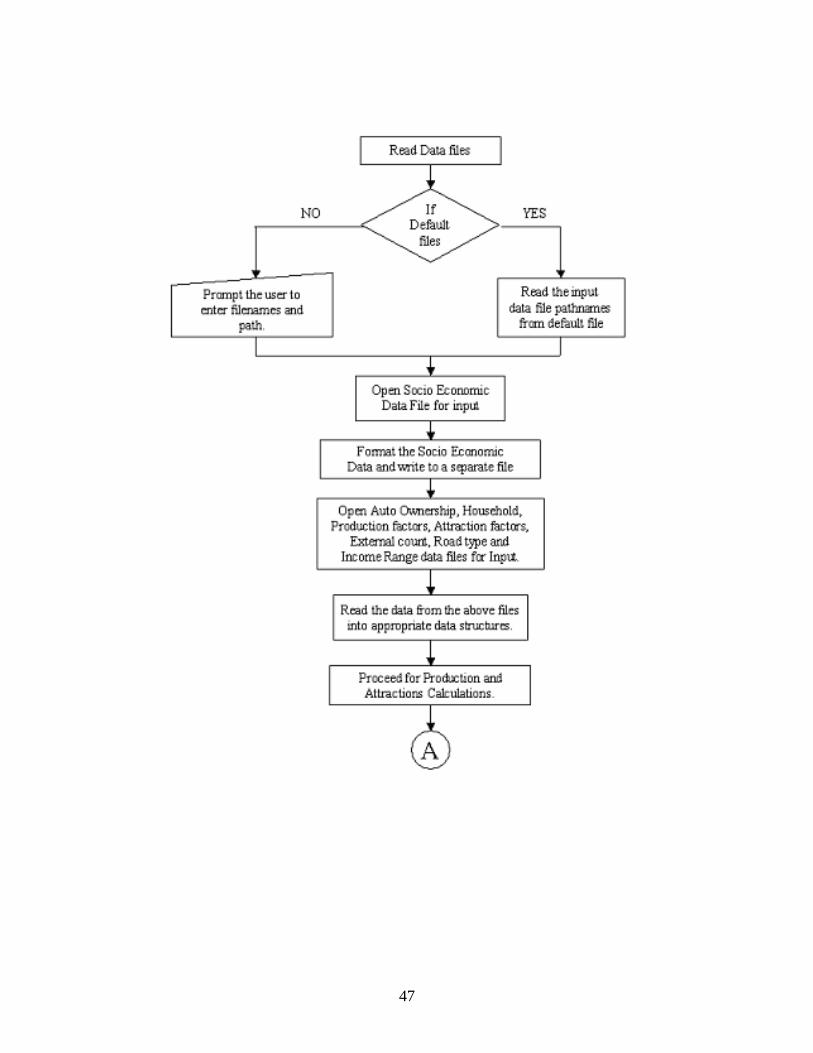
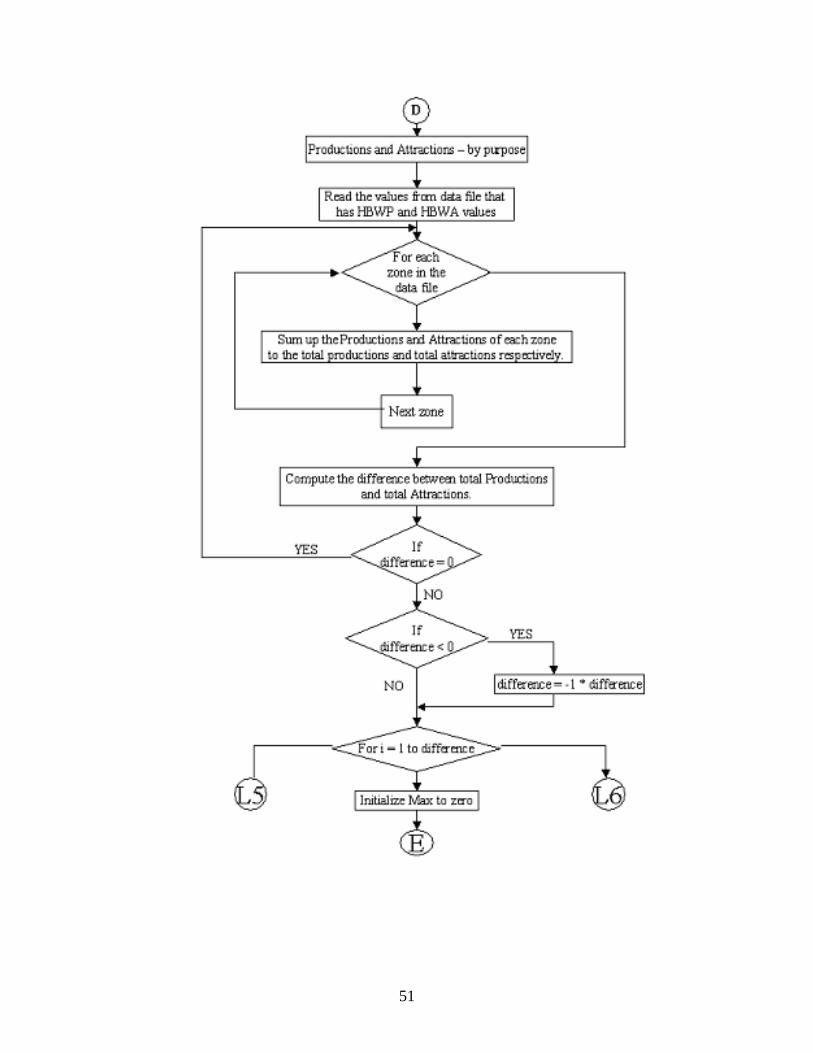
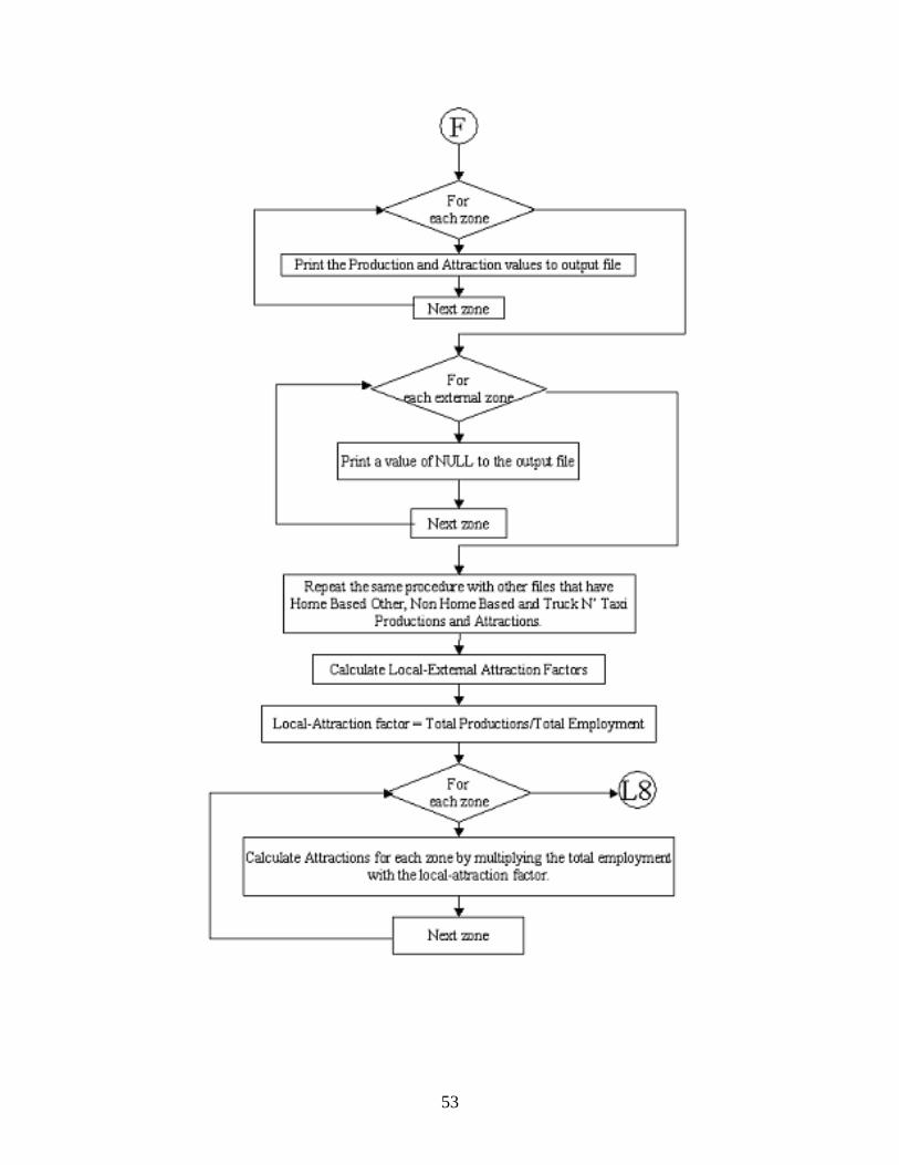
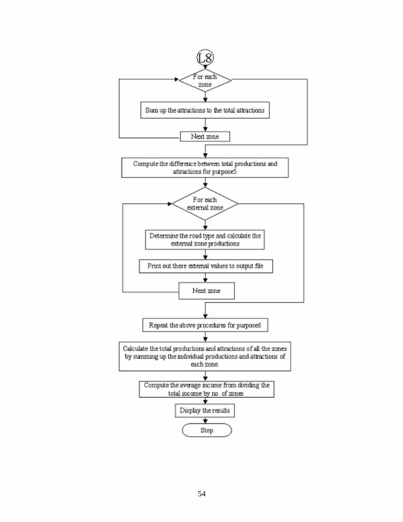
Appendix B Trip Generation Software Flowchart

47

48

49

50

51

52

53

54

55