an-examination-of-the-linkages-between-money-management-and-trading-goals-a-research-paper_by_giuseppe-basile...

An examination of the linkages between money

management and trading goals Research Paper

by Giuseppe Basile

Units for Fixed Amount

of CashNaive

Trading Rule(*)

Money Management Techniques(*)

Trading Goals

Monte Carlo

Simulator

Market Data(*)

Account SizeSub-Goal(*)

Trading Rule

application to

Market Data

MCS Method

Set Goals

Results to be

expected in

actual trading

Trading Simulator

MS Excel

3. Trading Simulations

1. Trading Data Generation

Trading Data Distribution

Calibration

Trading

Distribution

2. Trading Data Distribution Calibration

4. Comparison

Legend:

Data

Method

Input / Output

Process

Units for Fixed Amount of Cash

& Market’s Money

Learn to trade the Measured Moves trading method. Visit me at my blog: www.fibstalker.com.

Subscribe my free Newsletter to receive: weekly review videos, FibStalker View on Currencies,

Trading plans for the Euro-Dollar cross and the S&P500 index, articles on my trading method

and High Frequency Trading and Program Trading, from which I derive my trading edge.

WWW.FIBSTALKER.COM

© 2010-2012 [email protected] – all rights are reserved (find information on my biography at the end of this work)

https://elitefive.wordpress.com/trading-method/

http://www.fibstalker.com/

http://eepurl.com/pV6mL

http://www.fibstalker.com/

mailto:[email protected]

Blog: www.fibstalker.com

Twitter: @fibstalker

e-mail: [email protected]

2

An examination of the linkages between money

management and trading goals by Giuseppe Basile

© 2010-2012 [email protected] – all rights are reserved

Abstract This paper is a summary of a research study whose objective was to establish a linkage between money

management techniques (helping determine “how much” can be risked per trade) and trading goals.

Three money management techniques were examined and applied to the profitable “Turtle Soup”

trading system. Trading goals were split in three different sub-goals: downside protection, upside

potential and an opportunistic outcome. A uni-variate Monte Carlo simulation method was adopted

and a trading data distribution calibrated using known goodness-of-fit techniques and tests. The

study not only confirms that good money management techniques are able to modify the results of a

profitable trading system positively affecting trading performance, but it also demonstrates that, as a

result of such capability, money management techniques can be used to control achievement of trading

goals. In particular, different features of money management are able to separately affect the

achievement of different sub-goals. The paper concludes that a linkage between money management

techniques and trading goals exists, therefore selection of the latter is not disjoint from considerations

and choices made in the area of the former. This work also offers a generic, re-usable framework to

study the impact of money management techniques on trading performance, given any trading system.

Introduction

In trading two critical decisions must be made: the direction to trade (long or short) and the

amount to risk, strictly related to the size of the position. It has been already shown by

Lajbcygier and Lim (2007) that the “how much to risk” decision can affect trading

performance. This study builds on that result and introduces the concept of trading goals into

the picture. Particularly, it focuses on how money management links into, relates to and affects

the achievement of trading goals, which constitutes the main research question. Since money

management techniques affect trading performance intuitively they should also affect the

achievement of trading goals. Formal support for such seemengly straight forward observation

requires a thorough simulation as there are three aspects that must be taken into account: (1)

trading goals are more complex to characterize than a simple percentage return, and require the

use of event probabilities; (2) the role of the trading system in achieving goals; (3) how different

money management features can affect the achievement of specific sub-goals.

This study is organized around three main sections: Methodology, Methods and Empirical

Results. The methodology section presents the analytical framework created and used in the

study. The methods section presents information related to trading data, identification of

trading goals and sub-goals, trading system rules, a description of the money management

techniques adopted, trading data distribution to feed the Monte Carlo method and setups for

the trading simulations. A description of the empirical results obtained from the simulations

mailto:[email protected]




3

and related conclusions complete the study.

Methodology

Trading goals are defined by several sub-goals (or objectives) identified assuming a long-

term horizon. In implementing a trading strategy the traditional asset allocation approach was

not adopted, firstly because traditional strategies based on the portfolio selection theory and

practice frequently do not provide results aligned with traders’ goals; secondly, the intent of the

study was to focus on pure money management, i.e. sizing the position in trading, and studying

how it affects the achievement of traders’ goals, given a fixed trading system. The approach

selected in the study, similar to that found in (Lajbcygier and Lim, 2007) but employing

financial simulations, allowed the analysis of the effects of money management techniques on

trading performance, which can be directly linked back to traders’ goals. Trading goals can

directly be related to trading performance, because goals can be achieved, not achieved, or be

partially achieved based on the results, i.e. value of the account, during and at the end of the

trading horizon. Notice that trading goals are better defined in terms of probability of

“success”, i.e. the event of achieving a positive outcome, and “ruin”, i.e. the event of hitting a

negative, unwanted outcome. An approach that statically applies a trading system and money

management techniques to historical data would fail in producing information related to the

probability of meeting specific goals and would only allow gathering measures on what “has

happened” in the past, but not on what “could happen” in the future. Simple simulations on

past data are not capable to tackling the probability of events and not able to describe possible

“alternative futures” or outcomes. This is the reason Monte Carlo (MC) simulations were

adopted: they still rely on data from the past but used to dynamically generate possible future

scenarios.

Considering the context of the study and in recognition that proper money management is

as important or indeed more important than the entry or exit rules provided by the trading

system, the latter plays a secondary role. The minimal requirements for the adopted trading

system were to: (1) be profitable on the selected market data; (2) be based on TA; and (3) easy

to implement. An effective model to simulate real trading outcomes, dynamically using past

data, should produce trading results similar to those obtained in actual trading. The comparison

of the results of the simulation and the trading goals established in advance would then allow

gathering empirical results to help addressing the target of the investigation.

The adoption of the Monte Carlo (MC) simulations avoids substantial problems which

present in historical simulations, the most important being the fact they can only reflect the

range of observed historical outcomes, along with the related truncation bias. MC method

however is more complex and its results depend on the quality of the probability distribution

used to model trading outcomes. As only one market instrument, a US stock index ETF, was

referenced in the study a mono-dimensional or uni-variate distribution was adopted, considered

time-invariant. This is a limitation as markets could change in the future affecting the shape or

parameters of the distribution, but that could be mitigated using a different trading system,

maintaining the stability of the results of this study. Another limitation, which could not be

removed, was the assumption that samples drawn from the adopted distribution are

uncorrelated with the statistical variable’s past values. In the context of this study, this is

equivalent to assuming that any trade outcome can be drawn at any time, thus negating the

evidence that the underlying market could be in a particular state, in which certain outcomes




4

are more probable than others. One such states is a market trending for prolonged periods of

time, as witnessed in the 1982-2000 bull market or, more recently, in the period between March

2009 and May 2011. The extent to which the distribution calibration, i.e. the process of deriving

the probability distribution from the historical data series might, at least partially, reflect this

correlation is unknown. The assumption that samples are uncorrelated over time is known to

have the potential to distort the simulation to a variable extent depending on the type of asset,

frequency of observations, and the historical period examined.

The quality of the distribution obtained through the calibration process is critical for the

performance of the MC method and validity of results. The MC simulation method can

incorporate non-normal probability distributions and allows better estimates of downside risk

when compared to historical simulations. Macroeconomic indicators and related predictive

variables were not part of the study and improvements of MC simulations outcomes using

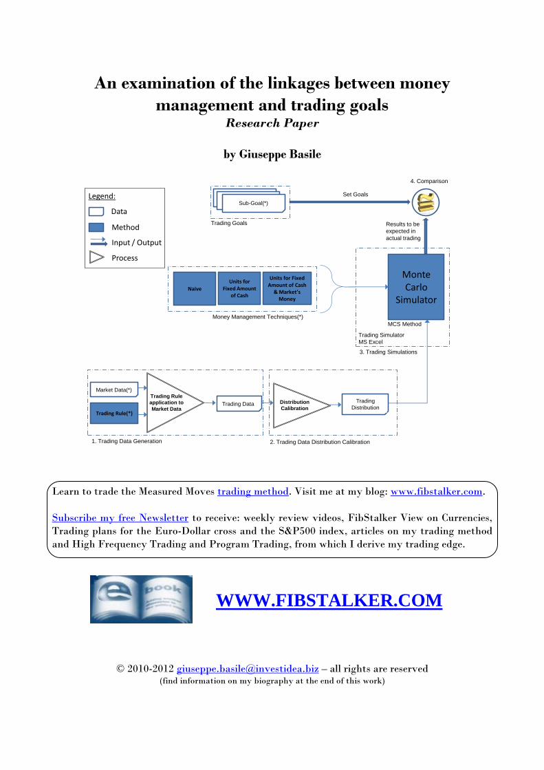
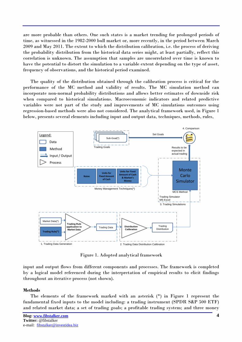
regression-based methods were also not considered. The analytical framework used, in Figure 1

below, presents several elements including input and output data, techniques, methods, rules,

Units for Fixed Amount

of CashNaive

Trading Rule(*)

Money Management Techniques(*)

Trading Goals

Monte Carlo

Simulator

Market Data(*)

Account SizeSub-Goal(*)

Trading Rule

application to

Market Data

MCS Method

Set Goals

Results to be

expected in

actual trading

Trading Simulator

MS Excel

3. Trading Simulations

1. Trading Data Generation

Trading Data Distribution

Calibration

Trading

Distribution

2. Trading Data Distribution Calibration

4. Comparison

Legend:

Data

Method

Input / Output

Process

Units for Fixed Amount of Cash

& Market’s Money

Figure 1. Adopted analytical framework

input and output flows from different components and processes. The framework is completed

by a logical model referenced during the interpretation of empirical results to elicit findings

throughout an iterative process (not shown).

Methods

The elements of the framework marked with an asterisk (*) in Figure 1 represent the

fundamental fixed inputs to the model including: a trading instrument (SPDR S&P 500 ETF)

and related market data; a set of trading goals; a profitable trading system; and three money




5

management techniques, to provide position sizing decisions for the trades generated by the

trading system. These elements are discussed in the following along with the statistical

distribution calibration and the setup for the trading simulations.

Market and Trading Data. Daily quotes of closing prices of the SPDR S&P 500 ETF fund

(symbol: SPY, AMEX) from January 1998 to January 2010 were used. In the tested period the

trading instrument moved within a wide range (low at $67.10 and a high at $157.52). The

period tested included the latter part of the great 1982-2000 bull market, the 2001-2002 bear

market, the 2003-2007 bull market, the 2008-2009 bear move and the latest market recovery

started in March 2009. This ensured that a wide set of market conditions, as well as,

participants’ behavior is represented by the selected market data.

Trading Goals. These are a significant input in the analytical framework (Figure 1) as they

are compared to the simulated trading results, i.e. the output from the MC method (Step 4).

Trading goals link trader objectives to risk management constraints and trading strategies. A

capital growth goal was selected and used throughout the study: this is made up of three sub-

goals (A, B and C), of which the first two (A and B) are mandatory and the third one (C) is

discretionary (optional). The first sub-goal A, deals with down-side protection, i.e. the

maximum amount of loss accepted by the trader with a specified probability, an event defined

as “ruin” with its likelihood, probability of “ruin”. This has been linked to the measure of the

worst final portfolio value using a 99% confidence interval, indicating a 1% probability that the

portfolio value will show a loss equal or smaller than the maximum amount of loss accepted.

This goal has the highest priority due to the importance of loss aversion behavioral bias showed

by traders.

Table 1. Sub-goals of targeted trading goals

The second sub-goal B deals with up-side potential, the very reason why financial resources

are put at risk. This corresponds to the minimum gain that can potentially be realized to

balance for the risks being taken. The event of reaching this minimum gain was defined

“success” and the related likelihood, probability of “success”. Sub-goal B is defined by two

objectives: (1) a minimal mean return; (2) a gain equal or greater than a defined threshold, with

a 20% probability of achieving it. A third, discretionary sub-goal C is related to the possibility

of gaining a “multiple” of the portfolio value at the end of the period, an opportunistic outcome

which could greatly improve performance results. Sub-goals are summarized in Table 1 above.




6

Sub-goals could not be defined without taking into account the efficiency of the trading

system, as well as, the actual opportunity represented by the intermediate-term price moves in

the selected market, during the referenced period of time. This information should only be based

on trading and market data, before any simulation is made. The 40% mean gain objective of

sub-goal B was arbitrarily set as double the amount risked, i.e. 20% of the initial account size,

as mentioned in sub-goal A. This is the expected outcome and a related probability was not

defined. The 60% upside potential sub-goal was also arbitrarily set to three times the amount

risked, along with an associated 20% probability. The opportunistic outcome has been defined

examining the “price potential” offered by the SPY market in the tested period, looking at the

monthly highs and lows. Table 2 below shows monthly low and high prices during the testing

period (January 1998 to January 2010) along with the returns of an hypothetical, “hindsight”

trading system capable of extracting the full potential of price moves in the selected market.

The total non-compound return is in the region of 355% and for its calculation a basic money

management (one share) was used, while transaction and tax costs were not taken into

consideration.

Table 2. Returns of a trading system capturing full SPY price potential

The ideal return of 355%, which it was assumed could potentially present in the future, has

been used to define the sub-goal C, the opportunistic outcome. Its probability of occurrence is

greater than zero, meaning that the goal is met if at least one trading simulation generates or

exceeds the ideal return.

Trading System. The “Turtle Soup” trading rule (Raschke and Connors, 1995), which trades

against the widely known Donchian 20-day channel breakout and aims at profiting from false

price breakouts, was adopted in the study. The trading system is simple and profitable on the

selected market data, it has only three rules, two entry rules and a timed exit rule; it generates a

sufficiently high number of trades, a requirement for the distribution calibration process; it

implements an effective, contrarian approach to a widely known system which has possibly

“stopped working” because of its diffusion among traders.

Figure 2 below provides the detailed rules of the “Turtle Soup” trading strategy, which take

trades both long and short. The strategy opens a long position if today’s closing price (CPt=0) is

below the minimum of low prices (LPi) of the last 20 days. Similarly, the strategy sells short if

today’s closing price is above the maximum of high prices (HPi) of the last 20 days. Entries are

always the next day, at market open price.




7

Figure 2. Entry and Exit rules of the “Turtle Soup” strategy

The number of shares, i.e. the position size (*), is always defined by the money management

technique that is “overlaid” on the trading strategy. The decision on “how much” is completely

independent from the decision on when to enter long/short or exit the market. To further

simplify the system, a timed exit rule was adopted which exits the current position at the close

of the 9th day after it is initiated, to complete a total of 10 days of duration. The two main

parameters are: (1) the channel days, cd=20; (2) the trade duration, td=10. The trading strategy

was not optimized in order to avoid data snooping.

Table 3. “Turtle Soup” strategy results on SPY market data

As showed by the report in the above Table 3, the trading strategy behaved well when

tested on the SPY market data, for the period January 1998 to January 2010, greatly

outperforming the buy and hold strategy. The strategy generated 178 trades (an average of

14.83 trades/year), had an overall reliability of 49.44%, an annual rate of return of 4.46% over

the 12-year period, with a return on capital of 71.29% outperforming the buy-and-hold return

of only 10.35%.

Money Management Techniques. Two main money management techniques, plus a

variation of the second one, were used: (1) Fixed Amount of Shares, a reference, naïve technique

trading a constant number of shares; (2) Units for Fixed Amount of Cash technique, suggested

in Tharp (2008), is based on the rule that one share is traded for every fixed amount of dollars in

the account; (3) Units for Fixed Amount of Cash and use of Market’s Money technique.

“Market’s money” is basically the profit extracted from the market at any moment, i.e. the

difference between the current account size and the initial account size, when positive or zero, if

negative. The idea is to use profits, when present, to proportionally increase risk. Making

reference to the Units for Fixed Amount of Cash technique, two different cash amounts can be

used in relation to the trading capital (own initial capital) and the market’s money (profits). In

this case, a smaller amount of cash per unit would be used with relation to profits, thus




8

increasing the position size (leveraging effect) by risking more than with technique (2), but only

in presence of profits. In absence of a profit the market’s money technique reverts to the Units

for Fixed Amount of Cash with no leverage effect. Although more complex money management

techniques could be used, including Optimal-f or LEED and others, imposing even more

emphasis on position sizing, simpler methods able to dynamically change the trade size were

deemed enough to show the linkages between money management and trading goals.

Trading Data Distribution Calibration. The Monte Carlo (MC) simulation of trading requires

finding the statistical distribution from which trades outcomes would be drawn. This was

obtained by finding the best fit for the sample of trades generated by the trading system on the

selected SPY ETF’s market data. The process to generate the data sample (called trading data)

for further calibration is represented by Step 1 (Trading Data Generation) in Figure 3 below.

Figure 3. Portion of the analytical framework for distribution calibration

Step 1 of the process applied the trading system rules to market data to obtain a sequence of

178 trades outcomes, expressed in positive (profits) and negative (losses) dollar amounts, the

trading data. Subsequently a technique known as distribution calibration (Step 2) was

employed to identify the statistical distribution that would best fit the trading data. Three

statistical tests called Chi-square goodness-of-fit, the Anderson-Darling and the Kolmogorov-

Smirnov tests were used. The Chi-square tests if the trading data comes from a population with

a specific univariate distribution (e.g. Normal, Logistic, Exponential, Triangular, Weibull,

Uniform, ect.), while the other two methods are employed to obtain confirmation. The outcome

of the calibration process is showed in Figure 4 below. A Normal distribution with parameters

mean=0.43253 and stddev=3.814 was the best fit for the trading data sample and the tests

confirmed the choice of the distribution shape with a 95% level of confidence, overall indicating

a model that would be wrong less than 25% of the times. Further confirmation was provided by

the study of the probability plot (Chambers et al., 1983), a graphical technique (not shown) for

visually assessing whether or not a data set follows a given distribution such as, for instance,

the Normal distribution. Samples withdrawn from the distribution identified represent trade

outcomes for one share traded, expressed in positive (gains) and negative (losses) dollar

amounts.

Trading Simulations Setup. Three models where created to simulate sequences of 178 trades,

the outcomes of a trading period 12 years long, represented by profits/losses figures withdrawn

from the calibrated Normal distribution. Results were obtained executing 100 runs of 10,000

simulations each, for each sequence of 178 trades. An initial account size of $100,000 was

assumed. Several simulation runs were executed with different techniques and parameters

relating to money management. Such parameters included the Fixed Number of Shares in the




9

naïve technique, the Fixed Amount of Cash/share in the Units per Fixed Amount of Cash

technique and the additional multiplier parameter for the Market’s Money variation.

Figure 4. Fit comparison between sample data (Input) and distribution (Normal)

In each simulation run the following measurements were produced and recorded: minimum

account value, mean account value, maximum account value, 1% percentile account value and

80% percentile account value. As each simulation produced 100 sets of results, one for each run,

two functions were applied to such sets to extract a meaningful figure for the account value

associated to the simulation: low(est) and high(est), chosen to correlate the simulation outcomes

with the trading goals. As a result the following measures were observed and recorded: lowest

minimum account value, lowest mean account value, highest maximum account value, lowest

1% percentile account value and lowest 80% percentile account value. Note that the lowest 1%

percentile account value relates to the downside protection sub-goal A; the lowest mean account

value and the lowest 80% percentile account value (corresponding to the 20% probability)

relates to the two objectives of the upside potential sub-goal B; and, finally, the highest

maximum account value relates to the opportunistic outcome sub-goal C. Only trading costs

($0.006 / share) and slippage ($0.01 /share) were considered in the simulations, while taxes were

not considered.




10

Empirical Results

In this section the results of the simulations are discussed. For the naïve money

management techniques only a summary of the results is provided due to its simplicity and

straightforwardness of related, expected outcomes.

Results of Fixed Amount of Shares technique (naïve technique). The parameter

corresponding to the Fixed Amount of Shares used in this trading simulation was iteratively

increased from 350 to 450, in increments of 10. Simulation showed that 420 shares is the highest

value offering the highest value for the mean and 80% percentile account value, while

guaranteeing a 1% percentile account value above $80,000 (thus satisfying sub-goal A). When

increasing the number of shares, however, observed results do not satisfy the downside

protection goal, producing a 1% percentile account value smaller than $80,000. As it can be

easily imagined, the naïve money management technique allows for a mild protection from

downside but it does not allow achieving the mandatory upside potential sub-goal B, and the

discretionary sub-goal C. On the upside, no simulation was able to reach the $250,000 mark.

Therefore it can be concluded that the use of this money management technique offered a

maximum return below 150%.

Results of Units for Fixed Amount of Cash technique. The parameter corresponding to the

Fixed Amount of Cash/unit used in this trading simulation was iteratively increased from $190

to $270, with $10 increments (meaning one share traded for every x dollars, with x being the

value of the parameter). In table 4 below that summarizes simulation’s results , $240/share was

the lowest figure offering the highest value for the mean and 80% percentile account value,

while guaranteeing a 1% percentile account value above $80,000 (thus satisfying sub-goal A).

Above $240/share, the money management technique facilitates meeting the downside

protection sub-goal A but does not satisfy either of the other two sub-goals (B and C). At

$230/share, the technique produces an 80% percentile account value above $160,000, partially

satisfying sub-goal B (i.e. gain 60% with a probability of 20%). Below $230 / share the

technique always achieves both objectives of sub-goal B (upside potential) and, below

$220/share also the discretionary sub-goal C. It is noteworthy that at $200/share the highest

account value generated was very close to meeting Sub-goal C. This is considered a simulation

run anomaly as Sub-goal C was satisfied with parameters of $210/share and $190/share.

Table 4. Simulation results for the Units for Fixed Amount of Cash technique

This money management technique can easily generate returns satisfying sub-goals B and C,

but it can only do it at the expense of risk management. When the downside protection sub-goal

A is enforced, the technique cannot generate the gains expected by the trader. The chart in

Figure 5 below shows the same data in Table 4 allowing a visual appreciation of the trend in the




11

main measures observed. As expected there is a negative relation between mean account value,

maximum account value, 80% percentile account value and the Fixed Amount of Cash

parameter, which is inversely related to the number of shares traded. As the amount of cash

increases, however, the drawdown decreases, as demonstrated by the increasing 1% percentile

and minimum account value lines.

Figure 5. Units for Fixed Amount of Cash technique: trends of main measures

Figure 6 below shows a summary trend chart for the trading scenario (178 trades) setting

the parameter to the $240/share value. The summary trend chart shows, in one place, the

collective outcomes of all 100 simulations.

Figure 6. Units for Fixed Amount of Cash technique: summary trend chart




12

For each simulation, the chart shows the lowest and highest account values (Min-Max,

green area) and the 1% and 99% percentile account values (1% - 99%, red area). The inner red

area (1% - 99%) shows that each simulation outcome respected the constraint imposed by sub-

goal A (downside protection), i.e. not generating 1% percentile account value smaller than

$80,000. The outer green area (Min-Max) shows potential minimum and maximum values for

the final account size. Notice that, on the downside, the final account value was never below

$50,000. On the upside, more than one simulation was able to exceed the $350,000 level and,

generally, all the simulations had a highest ending account value above $270,000, thus

generating a minimal return of 170%.

Results of Units for Fixed Amount of Cash and Market’s Money technique. The parameter

corresponding to the Fixed Amount of Cash/unit used in this trading simulation was arbitrarily

set to $240, the lowest value that guarantees sub-goal A (downside protection) in the previous

trading simulation. The second parameter, the shares multiplier, was iteratively increased from

0.9 to 1.9, with 0.1 increments. This parameter represents the amount of “leverage” allowed by

the presence of market’s money (i.e. profits), and it was used to calculate the overall number of

shares traded employing the formula: TRUNC{(account value/$240) x shares multiplier}.

Table 5 below shows the simulation observed results. It also shows that values existed for the

multiplier parameter enabling all the sub-goals (A, B and C) to be met, the lowest of such values

being 1.7.

Table 5. Simulation results: Units for Fixed Cash and Market’s Money technique

Values below 1.7 did not enable reaching the discretionary sub-goal C. Sub-goal B (upside

potential) could also be met for values equal or greater than 1.6. For values between 1.3 and 1.5

sub-goal B could only be partially met, with a probability of 20% of returns above 60%, i.e. an

80% percentile account value above $160,000. Thus the Units for Fixed Account of Cash and

Market’s Money technique was able to generate returns satisfying all the sub-goals, without

overlooking risk management.

The chart in Figure 7 below shows the data in Table 5 providing a way to visualize the trend

of the main measures for different values of the multiplier parameter. As expected there is a

positive relation between mean account value, maximum account value and 80% percentile

account value and the multiplier parameter, also positively related to the number of shares

traded. As the multiplier increases, however, the drawdown remains stable below the 20%

threshold, as demonstrated by the flat 1% percentile and minimum account value lines. This is

the result of having set a Fixed Amount of Cash parameter to $240, observed from the previous

simulation.




13

Figure 7. Units for Fixed Amount of Cash and Market’s Money: observed trends

Figure 8 below shows a summary trend chart for all 100 simulations in the trading scenario

using $240 for the Fixed Amount of Cash parameter and 1.7 for the multiplier parameter.

Figure 8. Units for Fixed Cash method and Market’s Money: summary trend chart

The inner red area (1% - 99%) shows that each simulation outcome respected the constraint

posed by the sub-goal A (downside protection), i.e. not generating 1% percentile account values

smaller than $80,000. The outer green area (Min-Max) shows potential minimum and maximum

values for the final account size. Notice that, on the downside, the final account value was never




14

below $60,000, similar to the case without use of market’s money. On the upside several

simulations showed results exceeding the $455,000 threshold (represented by the red line in

Figure 8), corresponding to the 355% opportunistic return related to sub-goal C. Generally all

the simulations had an ending account value above $350,000, thus generating a minimal return

of 250%.

Conclusions

The results show how different money management techniques are capable of affecting

trading performance, a confirmation of the findings of Laibcygier and Lim (2007). The choice of

the money management technique could greatly enhance the trading system performance

characteristics. Money management techniques could be used to control whether trading goals

were achieved, therefore a linkage between money management and trading goals could be

established, allowing a positive answer to the research question. In relation to the achievement

of trading goals, the study of the results of financial simulations provided evidence as to the

limitations of some of the money management techniques. This was despite the possibility to

partially modify their behavior using different values for their parameters. The study also

showed that some peculiar features of money management techniques were able to improve the

achievement of some of the sub-goals.

The first simulation showed that a simple money management technique was able to meet

the downside protection sub-goal A, related to the loss aversion behavioral trait (downside

protection), while it was unable to generate enough profits to reach the mandatory upside

potential B and the discretionary opportunistic outcome C sub-goals. Notice that, however,

such poor performance in achieving most of the goals is as indicative as the ability of achieving

all the goals, when establishing the existence of a link between the choice of the money

management technique and a set of trading goals. The second financial simulation showed that

using a variable position size (i.e. a variable number of shares) brought two main

improvements: firstly, it allowed the generation of much higher profits to meet the mandatory

upside potential B and the discretionary opportunistic outcome C sub-goals; secondly, it raised

the minimum account value obtained in the simulations, accomodating for better risk

management. However, increasing too much the number of shares traded would not allow

satisfying the all important downside protection sub-goal A. The study showed that when

adding the “market’s money” feature, accomodating for a variable, proportionally higher or

lower risk based on the portion of profits realized, the full set of trading goals could be achieved.

In particular, this feature allowed increasing the position size much more quickly than it would

have been possible with the basic technique. Trading this feature with a fixed amount of

cash/share able to meet the mandatory downside protection sub-goal A always allowed the

identification of an adequate multiplier parameter which would also help achieving the upside

potential B and the opportunistic outcome C sub-goals.

This study formally indicates that some relation does exist between the achievement of

trading goals and the money management technique and related parameters selected. In

particular, different features of the money management techniques are able to separately affect

the achievement of different sub-goals. For instance, a variable number of shares increasing or

decreasing with the size of the account can significantly boost performance while reducing risk.

Good money management techniques are able to modify the results of a profitable trading

system in order to positively affect trading performance. This implies that proper money




15

management is as important or even more important than the trading system itself, as also

demonstrated in other studies and practitioner’s works, including Laibcygier and Lim (2007),

Rayome and Jain (2008) and Tharp (2008).

Despite the assumptions and limitations illustrated in the work (assumptions on Monte

Carlo simulations, time-invariance, distribution calibration, trading goals definition, trading

system selection, ect.) some mitigations are believed to help preserving the validity of the

study’s results. Those include the use of a uni-variate distribution, absence of leverage – as the

use of margin was never assumed – that mitigates extreme negative outcomes (losing trades)

due to “fatter tails” reflected by empirical distributions or the inability of the trading system to

adapt to changing market conditions. The trading system can be considered a secondary aspect

to this study, not only because of the pursued objective, but especially in light of the evidence

that money management techniques can be considered more important than the system itself.

Finally, concerning the definition of some of the trading goals adopted, it could be safely

assumed that they sit somewhere in the broad spectrum of goals which can be linked back to

the variety of traders’ risk tolerances. Within the context of such a stronger assumption we can

conclude that a linkage between money management techniques and trading goals exists.

This study gives a different perspective to the importance of money management by linking

it directly to trading goals. Not a new perspective, in fact, but one investigated more by

practitioners than in the academic environment as highlighted by the limited work focusing on

the area of money management, also confirmed by Laibcygier and Lim (2007). The results can

be of interest to portfolio and wealth managers, professional and retail traders, brokers. Results

push for a better understanding of proper money management techniques, in conjunction with

the trading strategy adopted to meet established goals. The study might also be of interest to

financial planners who have the responsibility to explain to clients when their expectations

exceed the effectiveness of known trading strategies in the context of current market conditions,

or whereas they are not compatible with implied risk probabilities as evidenced by financial

simulations.

Bibliography

- Basile, Giuseppe (2010), “An Examination of The Linkages Between Money

Management and Investing Goals”, dissertation submitted for the degree of Master of

Arts in Finance, National College of Ireland, Oct 2010

- Chambers, John; William Cleveland; Beat Kleiner; Paul Tukey, (1983), Graphical

Methods for Data Analysis, Wadsworth.

- Lajbcygier, Paul and Lim, Eugene (2007), “How Important Is Money Management?”,

Institutional Investor; Jun 2007 Supplement, Vol. 41, p. 58-75 [Online] Available at:

http://wfxsearch.webfeat.org/wfsearch/search [Accessed 10 September 2009].

- Raschke Bradford, Linda and Connors, Laurence A. (1995), Street Smarts: High

Probability Short-Term Trading Strategies, M. Gordon Publishing Group, Inc.

Practictioner’s book.

- Rayome, David L. and Jain, Abhijit (2008), “Technical Trading: Donchian Channels

and Soybeans I”, Review of Business Research, Vol. 8, No. 4, 2008, pp. 187-198

- Tharp, Van (2008), Definitive Guide to Position Sizing. International Institute of

Trading Mastery, Inc. 102A Commonwealth Ct, Cary NC. Practitioner’s book




16

Who’s Giuseppe Basile

I earned a Masters in Computer Engineering in 1999 at the University "La Sapienza" of Rome,

Italy. Before I became a full-time futures and forex traderI worked at Accenture, a multi-

national management and IT consulting company, as an Information System Architect and IT

Project Manager. In a 10-year period of employment I travelled extensly in several Europena

countries. I developed an interest for the markets in 2001 but only in 2004 I have definitely

decided to get fully involved and become a trader and mentor. That decision required, of course,

a lot of preparation and a total change of my own psychology. I have studied tents of books,

executed thousands of trades and made an even higher number of mistakes. I have also studied

with several sucess traders and mentors in UK, Europe and US.

From 2006 to 2010 I lived in Dublin, Ireland where I entered the CFA program and, in October

2010, earned a Masters in Finance at the “National College of Ireland”. At the beginnng of 2009

I left my job at Accenture to become a full-time trader. Today I am an active trader specializing

on the Euro FX currency futures contract traded on the CME. In addition to this, I keep

studying the markets and testing continuosly new trading ideas and money management

techniques, run a Blog, complete reseach papers and statistics analysis, I write books and teach

courses on futures and stocks trading. I became SIAT member in 2012 and presented my work

at the TraderFest in June, as well as, at TraderLink/SIAT in October 2012.

Chi e’ Giuseppe Basile

Mi sono laureato in Ingegneria Informatica nel 1999 presso l’Università "La Sapienza" di Roma.

Prima di diventare trader di futures a tempo pieno ho lavorato presso Accenture, una delle

multinazionali della consulenza, in qualità di architetto di sistemi informativi e project

manager. Nei 10 anni di lavoro dipendente ho viaggiato estesamente in diversi paesi europei. Ho

sviluppato un interesse per i mercati nel 2001 ma solamente nel 2004 ho definitivamente deciso

di diventare trader e mentore. Quella decisione ha richiesto, naturalmente, molta preparazione

ed un cambiamento completo della mia psicologia. Ho studiato decine di libri, eseguito migliaia

di trade e fatto un numero anche maggiore di errori. Ho inoltre studiato con diversi traders e

mentori di successo in Inghilterra, Europa e USA.

Dal 2006 al 2010 ho vissuto in Irlanda, a Dublino, dove ho intrapreso il programma CFA e

nell’ottobre 2010 ho conseguito un Master in Finanza presso il “National College of Ireland”.

All’inizio del 2009 ho lasciato il lavoro ad Accenture per diventare un trader a tempo pieno.

Oggi sono un trader attivo e specializzato sul contratto CME Euro FX currency futures. In

aggiunta studio e testo continuamente nuove idee di trading e tecniche di money management,

compilo lavori di ricerca ed analisi statistica, scrivo libri e sono relatore in corsi sul trading di

azioni e futures. Sono diventato socio aggregato SIAT nel 2012 e hi presentato parte del mio

lavoro al TraderFest di Desenzano in Giugno, e anche all’evento TraderLink/SIAT in Ottobre

2012.

http://www.accenture.com/

http://www.traderfest.it/

http://www.accenture.com/

http://www.traderfest.it/

an-examination-of-the-linkages-between-money-management-and-trading-goals-a-research-paper_by_giuseppe-basile...

Documents

Transcript of an-examination-of-the-linkages-between-money-management-and-trading-goals-a-research-paper_by_giuseppe-basile...