An Exact Bayes Test of Asset Pricing Models with ...pluto.huji.ac.il/~davramov/paper3.pdf · An...

Doron AvramovUniversity of Maryland

John C. ChaoUniversity of Maryland

An Exact Bayes Test of AssetPricing Models with Applicationto International Markets*

I. Introduction

Financial economists have derived equilibrium as-set pricing models such as the Capital Asset Pric-ing Model (CAPM) of Sharpe (1964) and Lintner(1965) and the consumption-oriented CAPM ofBreeden (1979). Subsequent work (e.g., Black,Jensen, and Scholes 1972; Fama and MacBeth1973; Breeden, Gibbons, and Litzenberger 1989)examined the empirical performance of uncondi-tional versions of these asset pricing models. Theempirical tests met with mixed results. More re-cent work examined versions of pricing modelsthat incorporate lagged variables such as the div-idend yield. Studying conditional models has boththeoretical and empirical appeal. Theoretically,Hansen and Richard (1987) show that, even ifthe unconditional CAPM fails, the conditionalCAPM could be perfectly valid. In addition,Campbell (1996) shows that any instrument thatforecasts future market returns or labor income

(Journal of Business, 2006, vol. 79, no. 1)B 2006 by The University of Chicago. All rights reserved.0021-9398/2006/7901-0011$10.00

293

* We want to thank seminar participants at the Federal ReserveBank of Atlanta, the Global Finance Conference in Beijing,the 2002Western Finance Association (WFA) meetings, the 2003American Finance Association (AFA) meetings, Gurdip Bakshi,Bjorn Eraker (WFA discussant), Lubos Pastor, NagpurnanandPrabhala, Rob Stambaugh, and especially an anonymous refereefor very helpful comments and suggestions. The usual disclaim-ers apply. Contact the corresponding author, Doron Avramov, [email protected].

This paper develops andimplements an exactfinite-sample test ofasset pricing modelswith time-varying riskpremia using posteriorprobabilities. Thestrength of our approachis that it allows multipleconditional asset pricingspecifications, bothnested and nonnested, tobe tested and comparedsimultaneously. Weapply our procedure tointernational equitymarkets by testingand comparing theinternational CapitalAsset Pricing Model(ICAPM) andconditional ICAPMversions of Fama andFrench (1998). Theempirical evidencesuggests that the bestperforming modelis the ICAPM withthe value premiumconstructed basedon global earnings-to-price ratio.

growth could be a priced factor for asset returns. Empirically, Lettauand Ludvigson (2001), among others, demonstrate that asset pricingmodels with conditioning information explain a substantially larger frac-tion of the cross-sectional variation in average returns than unconditionalmodels.The asset pricing literature also proposed various econometric ap-

proaches to testing asset pricing models. In particular, a multivariatefinite-sample test was introduced by Gibbons, Ross, and Shanken (1989).In addition, Shanken (1987), Harvey and Zhou (1990), McCulloch andRossi (1991), and Geweke and Zhou (1996) all developed small-sampleBayesian tests. These tests, however, are designed to test unconditionalmodels and not models that incorporate conditioning information. Withconditioning information, asymptotically valid asset pricing tests are avail-able, such as the cross-sectional approach of Fama and MacBeth (1973),the generalized method of moments (GMM) of Hansen (1982), and thedistance measure of Hansen and Jagannathan (1997), but finite sampletests are yet to be developed. This paper fills a gap in developing and im-plementing an exact finite-sample test of asset pricing models with condi-tioning information. Our test allows risk premia and potential asset pricingmisspecification to vary predictably in response to changing economicconditions.To our knowledge, this work provides the first exact finite-sample

test of asset pricing models with conditioning information. The methodintroduced here allows one to simultaneously test and compare the per-formance of multiple-asset pricing specifications, both nested and non-nested. There are other advantages to using our approach. For example,the test can be applied without explicit knowledge of the long-run (low-frequency) properties of the stochastic processes that generate excessstock returns, underlying risk factors, and information variables. Thus,the decision rule for evaluating model performance is not affected bythe possible presence of a unit root in lagged variables such as the div-idend yield.Bayesian methods of hypothesis testing and model selection, such as

the one employed here, lead to a test statistic that comprises both an in-sample goodness-of-fit measure and a penalty term for model complexity(seeKass andRaftery 1995). Since a higher-dimensionalmodel that nestsa smaller model always fits the data at least as well, if not better, as thesmaller model, the presence of a penalty term in the test statistic guardsagainst overfitting the data, which may occur if models are evaluatedonly on the basis of goodness of fit. Thus, our Bayesian procedure that pe-nalizes model complexity helps prevent the inclusion of excess, uselessfactors in linear factor models. Indeed, implicit in the trade-off betweengoodness of fit and model complexity is the assertion that, since all equi-librium pricingmodels aremere approximations of the phenomenon understudy, the use of a larger, more complex pricing model is justified over a

294 Journal of Business

more parsimonious one only if the former can be shown to be significantlybetter at fitting the data than the latter.To illustrate the broad applicability of our finite-sample test, we apply

our procedure in an international asset pricing context. We study fivecompeting asset pricing specifications. These are the conditional versionsof the international CAPM (ICAPM) and four ICAPM’s of Fama andFrench (1998), each of which consists of the global market portfolio andthe global value premium. As in Fama and French, the global value pre-mium is formed as the return differential between (1) high and low book-to-market stocks, (2) high and low earnings-yield stocks, (3) high andlow cash-flow-to-price stocks, and (4) high and low dividend-yieldstocks. Whereas, under the CAPM, the global market portfolio is con-ditionally mean-variance efficient, under the Fama and French model,some combination of the global market and global value premium port-folio lies on the conditional minimum-variance boundary of risky assets(e.g., Roll 1977; Hansen and Richard 1987; and Huberman and Kandel1987).

In the empirical implementation, each of the 10 data generatingmodels,which consist of the restricted and unrestricted versions of the 5 assetpricing specifications noted earlier, are assigned equal prior probability.When such ‘‘neutral’’ initial beliefs are combined with the sample, theupdated beliefs strongly support the international CAPM and ICAPM. Inmost cases, the posterior probabilities in favor of specifications that allowfor asset pricing misspecification are substantially lower than those formodels where asset pricing restrictions are assumed to hold exactly. Aninteresting result coming out of the cross-model comparison is that thebest performing asset pricing specification is the Fama-French modelwith value premium constructed based on earnings yield. Remarkably,this model outperforms the other Fama-French models, even in somecases where the test assets are portfolios that are not sorted on earningsyield but on other equity characteristics, such as book-to-market, cash-flow-to-price, or dividend-to-price ratios, where a priori one would expectcompeting models to have a decisive advantage. In contrast to the earn-ings yield specification, the book-to-market-based ICAPM does not per-form nearly as well in our series of horse races, recording zero or near zeroposterior probabilities for all but a few of the test assets studied.The remainder of the paper proceeds as follows. Section II introduces

a generic form of conditional asset pricing models, discusses its testableimplications, and describes our Bayesian approach to hypothesis test-ing, model selection, and model combination. Section III presents exactformulae for both restricted and unrestricted factor model specificationsand states our decision rules for selecting among competing models.Section IV presents empirical results, and we offer some concludingremarks and ideas for future research in Section V. Unless otherwisenoted all derivations are presented in the appendix.

295Asset Pricing Models for International Markets

II. Evaluating Conditional Asset Pricing Models

A. Deriving Testable Restrictions

To evaluate asset pricing models with conditioning information, we firstspecify the dynamics of stock returns, underlying factors, and informa-tion variables. In particular, let rt denote an N-vector of returns on testassets in excess of the risk-free rate; let ft denote a K-vector of returns onportfolio-based factors, such as a claim to total wealth; and let zt denoteanM-vector of conditioning information, such as the dividend yield. Wedescribe the multivariate form of the data-generating process for excessreturns, factors, and predictive variables as

Y ¼ X Aþ U ; ð1Þ

where

Y ¼

r10; f1

0; z10

..

.

rT0; f T

0; zT0

2664

3775; ð2Þ

where X ¼ ½iT ;Z�1�;Z�1 ¼ ½z0; . . . ; zT�1�0; iT is a T�1 vector of ones, Tis the sample size, andU is a T � ðN þ K þMÞmatrix of the regressiondisturbances. It is assumed that the variance covariance matrix of the dis-turbances (denoted by S) is constant over time. For the analysis that fol-lows, we make the following partitions Y ¼ ½R;F; Z�; A¼ ½AR;AF ;AZ �;andU ¼ ½UR;UF ;UZ �;whereR¼ ½r1; . . . ; rt�0; F ¼ ½ f1; . . . ; fT �0; and Z ¼½z1; . . . ; zT �0. Asset pricing models impose testable restrictions on the mul-tivariate system in equation (1). Next, we derive those asset pricing re-strictions and develop a novel procedure for testing the restrictions.Consider now a beta factor model obeying the form

Eðrtjzt�1Þ ¼ aðzt�1Þ þ bEð ftjzt�1Þ; ð3Þ

where aðzt�1Þ is an N-vector of mispricing across assets with respect tobenchmark portfolios under consideration, and b is an N� K matrix offactor loadings. It is assumed that aðzt�1Þ linearly depends on informa-tion variables observed at time t � 1, thereby taking the form aðzt�1Þ ¼G 0xt�1; where G is an ðM þ 1Þ � N asset mispricing matrix and xt�1 ¼½1; z0t�1�0. The matrix of factor loadings is b ¼ ½Covfrt; ft 0jzt�1g� �½Covf ft; ft 0jzt�1g��1

. As noted earlier, the matrix S is assumed constantover time, thereby the conditional beta does not varywith time and is equalto the fixed quantity SRFS�1

FF ; where SRF ¼Covfrt; ft 0jzt�1g and SFF ¼Covf ft; ft 0jzt�1g. That is, the conditional beta can be directly com-puted from the distinct partitions of the covariance matrixS. In adopting


a constant beta framework, we follow the work of Campbell (1987) andothers. We note that, although treating the conditional beta as fixed haspotential costs, such a treatment has the advantage that it leads to a moreparsimonious specification that avoids the need to estimate additional setof parameters characterizing the evolution of beta variation. Moreover,Ghysels (1998) shows that, if the dynamics of beta are misspecified,serious pricing errors may result. Those pricing errors could be larger thanthose with a constant beta model.It should also be noted that, while this paper adopts a beta pricing

representation in conducting empirical analysis of asset pricing models,an alternative approach, the so-called stochastic discount factor (SDF)approach, instead takes a pricing kernel representation of pricing models.An example of an interesting recent paper that takes this approach isLettau and Ludvigson (2001), which documents the importance of scalingthe pricing kernel parameters by information variables. As has been ar-gued forcibly by Kan and Zhou (1999, 2003), a main advantage of thebeta pricing approach is that, because it incorporates a fully specifiedmodel, it is at least as efficient as the SDF approach, if not more so.Indeed, within a conditional framework, full specification of the dy-namics of asset returns and their dependence on information variables islikely to lead to rather substantial efficiency gains. In addition, we notethat the constant beta paradigm is not at odds with time-varying pricingkernel parameters. To illustrate this point, consider a pricing kernel obey-ing the linear form xtþ1 ¼ aðztÞ þ bðztÞ0 ftþ1. FollowingCochrane (1996),the equivalence between a beta pricing model and a pricing kernel speci-fication implies that

aðztÞ ¼ 1=rft½1þ lðztÞ0S�1FFlðztÞ�; ð4Þ

bðztÞ ¼ �1=rftS�1FFlðztÞ; ð5Þ

where rft is the 1-period conditionally riskless T-bill and lðztÞ ¼ aF þaFzt; and where theK�1 vectoraF and theK�Mmatrix aF are the cor-responding partitions of AF . Observe that time-varying risk premia lðztÞand time-varying riskless rate imply time-varying pricing kernel parame-ters, even when beta is fixed.When factors are portfolio based, one can obtain the following rela-

tionship between several blocks in the regression coefficients A and Sand the mispricing matrix G:

AR ¼ Gþ AFS�1FFSFR: ð6Þ

This relation is similar to that derived by Campbell (1987), except that,here, factors are prespecified as opposed to being latent, as in the frame-work of Campbell. Observe from equation (6) that, if expected return


variation is due to common risk factors (G = 0), the predictable com-ponent of returns is a linear transformation of the predictable componentof returns on factor-mimicking portfolios, with the transformation matrixbeing equal to beta. This relationship has an intuitive appeal. If all theassets in the economy are priced by a lower dimensional set of K bench-mark positions, then the problem of exploring the predictability of returnson N various securities having random payoffs boils down to exploringthe predictability of benchmark asset returns. Differences in predictabil-ity across assets, reflected through distinct columns in the matrix AR; areattributable to different loadings on the benchmark positions. The pres-ence of equity mispricing breaks this relationship, in that cross-sectionaldifferences in predictability are attributable not only to different factorloadings but also tomodelmispricing, whosemagnitude can differ acrossthe test assets.A hypothesis that favors the prevalence of an asset pricingmodel, such

as the CAPM or the Fama and French (1993, 1996, 1998) multifactormodels, restricts all elements of aðzt�1Þ to be equal to 0 at every timeperiod. In that case, the error terms obtained by regressing excess returnson factor-mimicking portfolio returns are not priced. To test the zero-intercept restrictions, we formulate asset pricing restrictions as a sharpnull hypothesis:

H0 : G ¼ 0 if and only if aðzt�1Þ ¼ 0 for all t;

H1 : G 6¼ 0 if and only if there is a t such that aðzt�1Þ 6¼ 0: ð7Þ

Under the null hypothesis, the time variation in expected returns is drivenby economywide risk factors only. Under the alternative, time-varying ex-pected returns can be explained, among others, by under- or overpric-ing. For example, DeBondt and Thaler (1987), Lakonishok, Shleifer, andVishny (1994), and Haugen (1995) attribute the value premium to over-reaction to corporate performance. The notion is that financial market par-ticipants undervalue distressed stocks and overvalue growth stocks.Whenmispricing is corrected, high-value stocks have high returns relative togrowth stocks. This correction governs stock return predictability.

B. A Bayesian Method for Hypothesis Testing and Model Selection

We evaluated the validity of the multivariate restrictions formulated inequation (7) using a hypothesis testing approach based on the Bayesianposterior odds (or, equivalently, the Bayes factor when prior model prob-abilities are taken to be equal, as explained later). To describe this ap-proach, we consider the case where there are L competing models (orhypotheses), denoted by

Mi : data has density f ðDjui;MiÞ; i ¼ 1; . . . ; L; ð8Þ


where D stands for the data and ui2Qi is the unknown parameter vectorof model Mi. Hypothesis testing from a Bayesian perspective proceedsby computing the posterior probabilities with each of the alternativemodels via Bayes’s theorem to yield the formula

PðMijDÞ ¼pðMiÞmðDjMiÞPL

i¼1

pðMlÞmðDjMlÞ; ð9Þ

where pðMlÞ gives the prior model probability of Ml and mðDjMlÞdenotes the marginal density (or the marginal likelihood) of the dataunder Ml. The marginal likelihood can be represented by the integralexpression

mðDjMlÞ ¼ZQl

f ðDjul;MlÞpðuljMlÞdul; ð10Þ

with pðul jMlÞ denoting the (proper) prior density of the parameter vec-tor ul under model Ml. Pairwise comparison between two models (say,Mi andMj for i 6¼ j) then can be conducted using the posterior odds ratio:

PðMijDÞPðMjjDÞ

¼ pðMiÞmðDjMiÞpðMjÞmðDjMjÞ

: ð11Þ

Looking at expression (11), we note that the factor pðMiÞ=pðMjÞ issimply the prior odds ratio ofMi toMj. We can also defineBij; the Bayesfactor for testingMi againstMj; as the posterior odds ratio over the priorodds ratio, so that in light of equation (11), the Bayes factor is simply theratio of the respectivemarginal likelihoods. Hence, the Bayes factor can beinterpreted as the odds forMi relative toMj after the prior odds ratio hasbeen updated by the information in the data. Note further that in the typicalempirical situation where the prior probability is taken to be the same foreach model, that is, where pðM1Þ ¼ pðM2Þ ¼ . . . ¼ pðMlÞ; the Bayesfactor is equivalent to the posterior odds ratio.A difficulty with computing the Bayesian factor is that, in the case

where the parameter space Ql is unbounded, one cannot take the priordensity pðuljMlÞ in the marginal likelihood expression (10) to be thatof a (improper) noninformative prior, such as the (improper) uniformprior (see Kass and Raftery 1995). To see the problem that the use of animproper prior creates, suppose we specify the uniform prior densitiespðuijMiÞ ¼ pi and pðujjMjÞ ¼ pj for modelsMi andMj; respectively.Then, the Bayes factor is

Bij ¼pi

pj

RQif ðDjui;MiÞduiR

Qif ðDjuj;MjÞduj

; ð12Þ


given that pi and pj are constants not depending on ui and uj. However,since the priors are improper (i.e., their densities integrate to infinityover the parameter spaces Qi and Qj), there are no unique normaliza-tion constants for these densities. Hence, we can just as well take as ourprior densities the alternative uniform densities pðuijMiÞ ¼ cipi andpðujjMjÞ ¼ cjpj; for constants ci and cj with ci 6¼ cj. The last prior spec-ifications lead to

Bij* ¼ cipi

cjpj

RQif ðDjui;MiÞduiR

Qif ðDjuj;MjÞduj

6¼ Bij; ð13Þ

for ci 6¼ cj. Thus, there is an indeterminacy with respect to the Bayesfactor specification.A common solution to the problem described previously, in the case

where the researcher does not wish to specify (proper) subjective priordensities for themodel parameters, is to split the total sample of dataD intotwo subsamples: a training sample, denoted D(t), and a primary sample,denotedD(�t). In the time series context we study here, there is a naturalordering of the data, so we can think of the training sample as compris-ing the first t observations of the data, or equivalently, comprising dataup to time t = t; whereas the primary sample comprises observationsfrom t = t þ 1 to T. The strategy commonly employed is to combinea (possibly improper) noninformative prior density, say, pN ðuijMiÞ;with data from the training sample to obtain a (proper) posterior density:

p½uijDðtÞ;Mi� ¼f ½DðtÞjui;Mi�pN ðuijMiÞR

Qif ½DðtÞjui;Mi�pN ðuijMiÞdui

; ð14Þ

where the size of the training sample must be chosen such that the den-sity p½uijDðtÞ; t;Mi� is indeed proper. This proper (posterior) densitythen is used as a prior density and combined with data from the primarysample to compute the posterior model probabilities for model compar-ison. Thus, analogous to expressions (9) and (10), we obtain

PtðMijDÞ ¼pðMiÞm½Dð�tÞjDðtÞ;Mi�P

l¼1

L

pðMlÞm½Dð�tÞjDðtÞ;Ml�; ð15Þ

where

m½Dð�tÞjDðtÞ;Ml� ¼ZQl

f ½Dð�tÞjul;DðtÞ;Ml�p½uljDðtÞ;Ml�dul;

ð16Þ


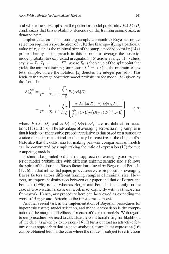
and where the subscript t on the posterior model probability PtðMijDÞemphasizes that this probability depends on the training sample size, asdenoted by t.Implementation of this training sample approach to Bayesian model

selection requires a specification of t. Rather than specifying a particularvalue of t, such as the minimal size of the sample needed to make (14) aproper density, our approach in this paper is to average the posteriormodel probabilities expressed in equation (15) across a range of t values,say, t ¼ T*; T* þ 1; . . . ; T *; where T* is the value of the split point thatyields theminimal training sample and T * ¼ ½T=2� is the midpoint of thetotal sample, where the notation [x] denotes the integer part of x. Thisleads to the average posterior model probability for modelMi given bythe formula

PAVGMi

¼ 1

T*� T* þ 1

XT*t¼T*

PtðMijDÞ

¼ 1

T*� T* þ 1

XT*t¼T*

pðMiÞm½Dð�tÞjDðtÞ;Mi�PLl¼1

pðMlÞm½Dð�tÞjDðtÞ;Ml�

8><>:

9>=>;; ð17Þ

where PtðMijDÞ and m½Dð�tÞjDðtÞ;Mi� are as defined in equa-tions (15) and (16). The advantage of averaging across training samples isthat it leads to a more stable procedure relative to that based on a particularchoice of t, since empirical results may be sensitive to the choice of t.Note also that the odds ratio for making pairwise comparisons of modelscan be constructed by simply taking the ratio of expression (17) for twocompeting models.It should be pointed out that our approach of averaging across pos-

terior model probabilities with different training sample size t followsthe spirit of the intrinsic Bayes factor introduced by Berger and Pericchi(1996). In that influential paper, procedures were proposed for averagingBayes factors across different training samples of minimal size. How-ever, an important distinction between our paper and that of Berger andPericchi (1996) is that whereas Berger and Pericchi focus only on thecase of cross-sectional data, our work is set explicitly within a time-seriesframework. Hence, our procedure here can be viewed as extending thework of Berger and Pericchi to the time series context.Another crucial task in the implementation of Bayesian procedures for

hypothesis testing, model selection, and model comparison is the compu-tation of the marginal likelihood for each of the rival models. With regardto our procedure, we need to calculate the conditional marginal likelihoodof the data, as given by expression (16). It turns out that an attractive fea-ture of our approach is that an exact analytical formula for expression (16)can be obtained both in the case where the model is subject to restrictions


of an asset pricing model, that is, G = 0 in equation (7), and where modelrestrictions are disregarded.The availability of exact formula for the marginal likelihoods is an

important advantage of our approach, since this allows exact posteriormodel probabilities to be computed without asymptotic approximation.In fact, growing evidence suggests that the asymptotically justified classi-cal hypotheses test performs poorly in finite samples. Ferson and Forester(1994), for example, providedMonte Carlo evidence suggesting that, withrespect to testing CAPMs, GMM-based tests may overreject for largesystemswithmany assets and suffer from low power for null models witha small number of risk factors. In contrast, finite sample tests of restric-tions of the form given in equation (7) within a multivariate linear systemcannot be readily implemented within a classical framework, even if theresiduals in the regression of excess returns on a constant intercept and aset of K factors are assumed to be Gaussian. In particular, note that theexact finite sample distribution of the classical likelihood ratio test fortesting the restriction (7) is complicated; and as far aswe know, no criticalvalues for such a test has ever been tabulated.Note also that, when the inference is conducted conditional on avail-

able data, one need not impose further conditions on the low-frequency(or long-run) behavior of the system given by equation (1). See Sims(1988), Sims and Uhlig (1991), and Phillips and Ploberger (1996) forfurther discussion on this point. In particular, we make no further as-sumptions about the order of integration of the time series variables rt; ft;and zt; so they may be either stationary processes or possibly unit rootprocesses. We believe this is an advantage of the approach taken here, aswe can proceed with inference about equilibrium asset pricing theorieswithout worrying about the difficult issues involved in pretesting the datafor unit roots and cointegration or possibly having to transform the data to‘‘induce’’ stationarity. Indeed, information variables such as dividendyield, term spread, and default spread are highly persistent and may in-volve a unit root.Furthermore, our approach could be attractive even from a sample the-

oretic or frequentist standpoint. It is well known that, given a fixed sig-nificance level, the classical approach to hypothesis testing (say, one basedon theWald or the likelihood ratio) is consistent only in the sense that theprobability of committing a Type II error vanishes as the sample size ap-proaches infinity; however, the probability of a Type I error for such a testdoes not approach zero, even in large samples. On the other hand, Bayesiantests based on the posterior odds or the Bayes factor can be shown undergeneral regularity conditions to be completely consistent, so that the prob-ability of both Type I and Type II errors vanishes asymptotically.Before leaving this section to discuss the explicit implementation of

our procedure, we want to note that, while many papers have tested assetpricingmodels, none pursues a framework similar to that developed here.


Shanken (1987), Harvey and Zhou (1990), and McCulloch and Rossi(1991) all developed posterior odds ratios to test the intercept restrictionas implied by factor based models. In addition, Geweke and Zhou (1996)entertained a finite-sample Bayesian approach for testing asset pricingmodels when factors are unobserved. However, these studies assumedthat expected returns are constant. In contrast, here, the intercept in theregression of excess returns on asset pricing factors and the price of betarisk could vary in response to changing economic conditions. Incorpo-rating time-varying expected returns is motivated on both theoretical andempirical grounds. Related to this work, Avramov (2002) derives pos-terior probability in a predictive regression framework but disregardingpricingmodel restrictions. In addition, Avramov (2004) exploits the assetpricing restrictions presented in equation (7) to form informative priorbeliefs about the extent of return predictability in an investment context.

III. An Exact Test of Asset PricingModels with Conditioning Information

Let MR denote the multivariate model (1) subject to the asset pricingrestrictions (7) and letMU denote the unrestricted version of (1). Then,in the case where pðMRÞ ¼ pðMU Þ ¼ 1=2;we obtain directly from ex-pression (17) the following formulas for PAVG

MRand PAVG

MU:

PAVGMR

¼ 1

q

� � X½T=2�t¼T*

m½Dð�tÞjDðtÞ;MR�m½Dð�tÞjDðtÞ;MR� þ m½Dð�tÞjDðtÞ;MU �

� �

ð18Þ

and

PAVGMU

¼ 1

q

� � X½T=2�t¼T*

m½Dð�tÞjDðtÞ;MR�m½Dð�tÞjDðtÞ;MR� þ m½Dð�tÞjDðtÞ;MU �

� �;

ð19Þ

where, in these expressions, q ¼ ½T=2� � T* þ 1 and where m½Dð�tÞjDðtÞ;MR� and m½Dð�tÞjDðtÞ;MU � denote the marginal likelihoodsunder MR and MU ; respectively.In the appendix, we give detailed derivations of exact expressions for

m½Dð�tÞjDðtÞ;MR� and m½Dð�tÞjDðtÞ;MU �. Specifically, the ap-pendix contains four propositions. Proposition 1 (3) derives informa-tive prior beliefs about unknown parameters pertaining to the restricted(unrestricted) specification. Proposition 2 (4) derives the marginal like-lihood of the restricted (unrestricted) specification. Following Harveyand Zhou (1990), McColluch and Rossi (1991), Kandel, McCulloch, andStambaugh (1995), and Geweke and Zhou (1996), we make the stan-dard Gaussian assumption on the errors of the multivariate regression


model (1). Of course, in light of the recent work by Tu and Zhou (2004), itwould be of interest to explore the robustness of the Gaussian assumptionhere by extending our approach to the case where the error distributionbelongs to the multivariate t family.Given analytic expressions for the marginal likelihoods, the average pos-

terior model probabilities PAVGMR

and PAVGMU

can be computed easily usingexpressions (18) and (19). It follows that a Bayesian test of asset pricingrestrictions can be implemented using either the odds ratio PAVG

MR=PAVG

MU

or its natural log transform ln ðPAVGMR

Þ � ln ðPAVGMU

Þ. Taking a loss func-tion that is symmetric with respect to Type I and II errors, the decision rulefor choosing the restricted model MR over the unrestricted model MU

can be stated as either

Choose MR over MU if PAVGMR

=P AVGMU

> 1 ð20Þ

or

Choose MR over MU if ln PAVGMR

� �.ln PAVG

MU

� �> 0: ð21Þ

Moreover, note that since PAVGMR and P

AVGMU

are (discrete) probabilities,satisfying the conditions PAVG

MR� 0; PAVG

MU� 0; and PAVG

MRþ PAVG

MU¼ 1;

we also have the decision rule:

Choose MR over MU if PAVGMR

>1

2: ð22Þ

(See Zellner 1971, pp. 294–97, for further discussion of Bayesian de-cision rules under symmetric loss function.)While expressions for the marginal likelihoods as given by equations

(A.15) and (A.25) in the appendix may appear to be cumbersome ourmethod, in fact, is easily implementable using a simple Matlab code,which is available from us on request.

IV. An Empirical Study: The Case of International Markets

To illustrate the broad applicability of our approach, we apply our pro-cedure in an international asset pricing context. We study five competingmodels, the international CAPM and four ICAPMs, which are the con-ditional versions of the unconditional models studied by Fama and French(1998). Inherent in the two-factor model is the assertion that the value pre-mium is compensation for a global risk factor missed by the global mar-ket portfolio. Under the CAPM restriction, the global market portfolio isconditionally mean-variance efficient. Under the two-factor model re-striction, some combination of the global market portfolio and the globalvalue premium lies on the conditional mean-variance frontier. In additionto testing each restricted model against its unrestricted counterpart, we


also conduct direct comparisons of all the models together on the basisof their posterior model probabilities. Note that such a comparison cannotbe done easily within a classical statistical framework, since the differentICAPM versions are mutually nonnested. In contrast, our procedure isespecially suitable for comparing both nested and nonnested models.In particular, the empirical analysis compares and evaluates asset pric-

ing models on the basis of their posterior probabilities. Any candidatemodel is represented by two competing return generatingmodels. One, thepricing model, implies zero intercepts in a multivariate regression of ex-cess returns on portfolio based factors. The other allows for the presence ofasset pricing misspecification, the extent of whichmay vary in response tochanging economic conditions. The appendix describes the derivation ofthe posterior probabilities for both the restricted and unrestricted specifi-cations. The posterior probability indicates the odds that stock returns aregenerated either by the restricted model underG = 0 in equation (7) or byits unrestricted counterpart. An interesting question is how to interpret themagnitude of the posterior odds ratio or the Bayes factor if the prior oddsratio is assumed to be unity. Jeffreys (1961) suggests a qualitative inter-pretation. According to him, the evidence against the alternative or in favorof the null is as follows. If the Bayes factor is between 1 and 3.2, the evi-dence does not justifymore than a baremention; if it is between 3.2 and 10,the evidence is substantial; if it is between 10 to 100, the evidence is strong;if it is greater than 100, the evidence is decisive.For the empirical implementation, we make three assumptions often

used in an international framework. First, world equity markets are per-fectly integrated, as in Korajczyk and Viallet (1989), Harvey (1991), andDumas and Solnik (1995). Second, investors are not concerned aboutdeviations from purchasing power parity (PPP). Otherwise, they wouldhedge against foreign exchange risk, and as a result, additional risk premiacorresponding to the covariances of returns with exchange rates wouldemerge. For example, Solnik (1974) shows that, when investors in inter-national markets face exchange risk, such risk should be priced, even in aworld otherwise similar to the unconditional CAPM. In our setting, for-eign exchange risk is not priced separately from the market risk, since thePPP assumption implies that investors do not perceive real changes inrelative prices. Third, as in Korajczyk and Viallet (1989), Harvey (1991),and Fama and French (1998), our empirical implementation takes theview of a global investor who cares about U.S. dollar returns.

A. Data

We study returns on market, value, and growth portfolios for the UnitedStates and 12major EAFE (Europe, Australia, and the Far East) countriesover the period 1975–2000. We adhere to the Fama and French’s (1998)portfolio definitions. HB/M and LB/M denote high and low book-to-market portfolios, respectively; HE/P and LE/P denote high and low


earnings yield portfolios, respectively; HC/P and LC/P denote high andlow cash-flow-to-price portfolios, respectively; and HD/P and LD/P de-note high and low dividend yield portfolios, respectively. All portfolioreturns are obtained from Ken French’s Web site.Following previous studies (e.g., Harvey 1991; Dumas and Solnik

1995), our list of instruments includes five variables: the excess rate ofreturn on the world index lagged 1 month, the January dummy, the U.S.term structure slope, the dividend yield on the U.S. value-weighted in-dex, and the 1-month rate of interest on a Eurodollar deposit. Indeed,some of the instruments used are local. This is due to Harvey (1991) andothers, who show that U.S. instruments have some power in predictingequity returns in foreign markets.Table 1 displays summary statistics across the 13 equity markets. We

report monthly excess returns on country-specific market, value, andgrowth portfolios. Excess returns are monthly in percent. Figures in

TABLE 1 Monthly Dollar Returns in Excess of U.S. T-Bill Rate for Market,Value, and Growth Portfolios: 1975–2000

Market HB/M LB/M HE/P LE/P HC/P LC/P HD/P LD/P

United States .80 1.08 .74 1.11 .69 1.03 .72 .90 .82(4.45) (4.32) (4.90) (4.66) (4.94) (4.28) (4.99) (3.82) (5.19)

Japan .61 1.07 .27 .96 .19 1.05 .20 .85 .36(6.67) (7.15) (7.09) (6.49) (7.27) (7.03) (6.76) (7.17) (7.01)

UnitedKingdom 1.09 1.27 .97 1.26 1.04 1.37 1.02 1.13 .96

(6.79) (7.28) (7.04) (7.00) (6.98) (7.17) (6.99) (6.71) (7.07)France .87 1.19 .77 1.09 .71 1.28 .76 1.15 .54

(6.66) (7.56) (6.76) (7.64) (6.93) (7.73) (6.88) (6.91) (7.23)Germany .68 1.09 .65 .73 .74 1.00 .37 .79 .64

(5.73) (6.08) (6.15) (6.00) (6.19) (5.79) (5.90) (5.67) (6.27)Italy .64 .61 .72 .60 .76 .88 .21 .90 .43

(7.80) (8.62) (7.79) (8.88) (7.99) (8.69) (8.05) (8.47) (8.02)Netherlands 1.01 1.07 .87 1.07 .79 .74 .87 1.10 .67

(5.13) (6.80) (5.40) (5.84) (5.79) (7.17) (5.60) (5.66) (6.18)Belgium .84 .97 .70 1.06 .79 1.12 .79 1.02 .70

(5.52) (6.42) (5.75) (5.69) (5.84) (6.21) (6.15) (5.91) (5.96)Switzerland .76 1.09 .68 .83 .73 .71 .69 .91 .67

(5.34) (5.87) (5.47) (5.78) (5.79) (6.05) (5.96) (5.81) (5.67)Sweden .98 1.20 1.00 1.32 1.04 1.08 1.09 1.26 1.00

(6.57) (7.93) (6.73) (7.29) (7.05) (7.73) (7.06) (7.27) (6.91)Australia .63 1.07 .39 1.10 .40 1.19 .27 .97 .46

(6.88) (6.91) (7.68) (6.42) (8.00) (7.11) (7.82) (6.36) (7.96)Hong Kong 1.44 1.52 1.25 1.71 1.36 1.76 1.35 1.76 1.52

(9.46) (11.46) (8.88) (10.36) (9.47) (9.72) (9.95) (9.60) (9.95)Singapore .84 1.34 .70 .98 .81 .93 .54 .67 .74

(8.22) (10.72) (7.93) (8.62) (9.00) (8.37) (8.22) (8.47) (9.25)

Note.—Value and growth portfolios are formed on book-to-market equity (B/M ), earnings to price(E/P), cash flow to price (C/ P), and dividend to price (D/P) in the same manner as described in Famaand French (1998). Also following Fama and French (1998), we denote value ( high) and growth ( low)portfolios using the letters H and L, respectively. The first number reported in each cell of table 1 is theannual average return of the given portfolio for each country, while the numbers in parentheses are thet-statistics for testing the null that the average return is no different from 0.


parentheses are the t-statistics for testing the null that the average return isno different from 0. Table 1 draws on table 3 in Fama and French (1998),except that the time series of returns spans the longer period 1975–2000.Table 1 shows some evidence in favor of the value premium in interna-tional returns. Firms with high ratios of book-to-market equity, earningsto price, cash flow to price, or dividend to price display higher averagereturns than firms with low ratios.

B. Results

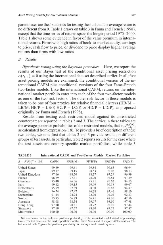
Hypothesis testing using the Bayesian procedure. Here, we report theresults of our Bayes test of the conditional asset pricing restrictionaðzt�1Þ ¼ 0 using the international data set described earlier. In all, fiveasset pricing models are examined: the conditional version of the in-ternational CAPM plus conditional versions of the four Fama-Frenchtwo-factor models. Like the international CAPM, returns on the inter-national market portfolio enter into each of the four two-factor modelsas one of the two risk factors. The other risk factor in these models istaken to be one of four proxies for relative financial distress (HB/M �LB/M, HE/P � LE/P, HC/P � LC/P, or HD/P � LD/P), as proposedoriginally by Fama and French (1998).Results from testing each restricted model against its unrestricted

counterpart are reported in tables 2 and 3. The entries in these tables arethe average posterior probabilities of the restricted models, that is, PAVG

MR;

as calculated from expression (18). To provide a brief description of thesetwo tables, we note first that tables 2 and 3 provide results on differentgroups of test assets. In particular, table 2 reports results for the casewherethe test assets are country-specific market portfolios, while table 3

TABLE 2 International CAPM and Two-Factor Models: Market Portfolios

R � F PAVGMR

� 100 CAPM FF(B/M) FF(E/P) FF(C/P) FF(D/P)

United States 99.69 99.61 99.84 99.63 96.94Japan 99.37 99.15 98.53 98.02 98.13United Kingdom 97.66 98.70 98.37 97.29 96.99France 98.29 97.61 98.20 97.84 97.39Germany 95.40 96.36 95.71 95.62 94.15Italy 99.12 99.15 99.09 99.18 99.07Netherlands 95.59 97.89 98.30 96.83 94.37Belgium 96.74 97.47 96.68 97.46 98.10Switzerland 91.14 94.24 92.90 92.02 92.33Sweden 55.95 56.29 66.41 47.26 42.56Australia 98.08 98.54 99.07 98.50 97.98Hong Kong 97.30 98.61 98.72 98.10 97.44Singapore 97.69 97.67 98.30 97.75 97.87Multivariate 100.00 100.00 100.00 100.00 100.00

Note.—Entries in the table are posterior probability of the restricted model stated in percentageterms. The test assets are the market portfolios of the United States and 12 major EAFE countries. Thelast row of table 2 gives the posterior probability for testing a multivariate system.


provides results where the test assets are global, as opposed to country-specific, characteristic-sorted portfolios. We also tested each restrictedmodel against its unrestricted counterpart for the cases where the testassets are taken to be various country-specific characteristic-sorted port-folios. However, we choose not to report these results here because theyare qualitatively very similar to the results reported in table 2, where thetest assets are country-specific market portfolios. These results, however,are available from us on request. Note also that, for both tables 2 and 3,the first column of each table gives results for the conditional version ofthe single-factor international CAPM;whereas the other four columns pro-vide results on the various two-factormodels, so that the numbers reportedin columns 2, 3, 4, and 5 correspond to results for the Fama-French modelwhose second factor is HB/M � LB/M, HE/P � LE/P, HC/P � LC/P,and HD/P � LD/P, respectively.Looking first at table 2, we see that, when the test assets employed are

country-specific market portfolios, our test results uniformly providestrong and unambiguous evidence in favor of conditional versions ofboth the international CAPM and the four Fama-French models relativeto models that allow for asset mispricing. Excluding Sweden, the smallestvalue of PAVG

MRrecorded across all countries and for the different asset

pricing models exceeds 91%, indicating strong evidence for the null hy-pothesis. Indeed, based on the decision rule (22), our Bayes procedurechooses the CAPM and the two-factor models over their unrestrictedcounterparts for each of the countries in table 2, with the exception ofSweden.In the case of Sweden, the posterior model probability PAVG

MRrecorded

for the Fama-French model whose second factor is HC/ P � LC/ P andthe Fama-French model whose second factor is HD/ P � LD/ P are bothunder 0.5 or 50%, indicating the possible inadequacy of these models inexplaining the market returns of Sweden. Moreover, PAVG

MRrecorded for

the CAPM, the Fama-French model whose second factor is HB/M�LB/M, and the Fama-Frenchmodel whose second factor isHE/ P�LE/ P

TABLE 3 International CAPM and Two-Factor Models: Global Characteristics

CAPM FF(B/M) FF(E/P) FF(C/P) FF(D/P)

HB/M 71.64 99.45 97.25 95.97LB/M 83.72 96.96 96.85 97.85HE/P 80.00 98.98 95.03 95.60LE/P 49.72 90.40 91.84 64.84HC/P 58.06 91.06 91.56 78.01LC/P 97.66 94.02 97.22 96.98HD/P 86.92 97.98 98.22 94.77LD/P 71.18 97.80 93.55 90.32

Note.—Entries in this table are (average) posterior probabilities of the restricted models stated inpercentage terms. Test assets are global characteristics-sorted portfolios.


are, respectively, 55.95%, 56.29%, and 66.41%; all of which are sub-stantially lower than the posterior model probabilities for the variousrestricted models recorded for other countries, which, as noted earlier,exceed 90%. The last row of table 2 reports results for the case where allthe country-specific market returns are tested simultaneously in a multi-variate regression framework. Here, the posterior probability in favor ofany pricing model studied is 100%. Hence, simultaneous testing yieldsstronger evidence in favor of the five asset pricing models over theirunrestricted alternatives.Our results somewhat differ from those of Fama and French (1998).

Whereas they reject the null hypothesis that the international CAPM isan appropriate model for the excess returns on country-specific HB/Mportfolios using the Gibbons, Ross, and Shanken (1989) GRS test; wefind the international CAPM to be an adequate model for these returnswhen judged against an alternative, unrestricted specification that allowsfor time-varying asset mispricing. It should be noted, of course, that anycomparison of our results here with those of Fama and French (1998)should be done with care, not only because of the difference in themethodology employed (i.e., Fama and French 1998 used classical hy-pothesis testing methods, while we use Bayesian testing procedureshere) but also because Fama and French (1998) do not account forpotential stock return predictability and our sample is 5 years longer.Turning our attention now to table 3, where the test assets are various

global characteristic-sorted portfolios, we note that, while the results pre-sented in this table still find in favor of the various restricted specificationsover their unrestricted counterparts, the evidence in favor of the CAPMvis-a-vis an unrestricted alternative appears to be weaker here, as judgedby the smaller value of its posterior model probabilities. Indeed, compar-ing the results from this table with those of the previous tables, we seethat, in contrast with the cases where the test assets are country-specificportfolios, the posterior model probabilities recorded for the CAPMare less than 0.8 or 80% for half of the eight categories of test assetsexamined.

Model comparison. Tables 4 and 5 exhibit posterior probabilitiesfor 10 data-generating models under consideration, the restricted andunrestricted versions of the 5 pricing models studied here. We assigneda prior probability of 10% to each specification. Figures reported in thetables are useful for both comparing the pricing abilities of the CAPMand four ICAPMs and incorporating model uncertainty in investment-based experiments. In particular, consider an investor whomust allocatefunds among multiple securities. The investor is uncertain about whichspecification, if any, is useful in pricing. That investor can use modelposterior probabilities for averaging across the 10 data-generating spec-ifications. Investment decisions can then be made based on a generalmodel that optimally nests the individual specifications using posterior


probabilities as weights. In this paper, we attempt to compare the em-pirical performance of various asset pricing specifications. Analyzinginvestment decisions in the presence of uncertainty about the correctasset-pricing specification and the set of predictive variables provides adirection for future work.Observe from tables 4 and 5 that, when neutral initial beliefs about

the pricing abilities of the five factor models are combined with thedata, the best performing model is the Fama-French whose secondfactor is (global) HE/P � LE/P (denoted by the symbol ME=P

R). Fo-

cusing first on table 4, where the test assets are country-specific marketand characteristic-sorted portfolios, we note thatME=P

Ris found to be the

best model for five of the nine categories of test assets examined. Infact , it is a bit surprising that, as judged by posterior model probability,ME=P

Rdoes a better job of explaining the returns on country-specific

LB/M portfolios than MB=MR , the Fama-French model whose second

factor is (global) HB/M � LB/M. Moreover, ME=PR also has slightly

higher posterior model probability than MCPR ; the Fama-French model

whose second factor is (global) HC/P � LC/P when the test assets are

TABLE 4 Model Comparison with Country-Specific Test Assets:Multivariate Case

MCR MC

U MB=MR MB=M

U ME=PR ME=P

U MC=PR MC=P

U MD=PR MD=P

U

Market .00 .00 .02 .00 97.12 .00 .01 .00 2.86 .00HB/M .00 .00 100.00 .00 .00 .00 .00 .00 .00 .00LB/M .00 .00 .77 .00 98.37 .00 .00 .00 .87 .00HE/P .00 .00 .00 .00 100.00 .00 .00 .00 .00 .00LE/P .00 .00 .00 .00 99.75 .00 .00 .00 .25 .00HC/P .00 .00 .02 .00 51.26 .00 48.72 .00 .00 .00LC/P .00 .00 .00 .00 .02 .00 99.98 .00 .00 .00HD/P .00 .00 .00 .00 .00 .00 .00 .00 100.00 .00LD/P .00 .00 .00 .00 16.68 .00 .00 .00 83.32 .00

Note.—Entries are (average) posterior model probabilities stated in percentage terms. Test assets aremarket portfolios and country-specific characteristics.

TABLE 5 Model Comparison with Global Characteristic-Sorted Portfolios asTest Assets

MCR MC

U MB=MR MB=M

U ME=PR ME=P

U MC=PR MC=P

U MD=PR MD=P

U

HB/M .00 .00 100.00 .00 .00 .00 .00 .00LB/M .00 .00 100.00 .00 .00 .00 .00 .00HE/P .00 .00 100.00 .00 .00 .00 .00 .00LE/P .00 .00 1.15 .00 79.97 .00 18.88 .00HC/P .00 .00 .00 .00 100.00 .00 .00 .00LC/P .00 .00 .00 .00 88.44 .00 11.56 .00HD/P .00 .00 2.24 .00 10.49 .00 87.27 .00LD/P .00 .00 2.51 .00 97.49 .00 .00 .00

Note.—Entries are (average) posterior model probabilities stated in percentage terms.


country-specific HC/P portfolios. The CAPM, on the other hand, doesnot compare favorably with the Fama-French ICAPM’s as a model forany of the country-specific test assets examined. Note also that return-generating specifications that permit asset mispricing are not at all sup-ported by the data. Applying the intuition of Jeffreys (1961) to our results,we record decisive evidence in favor of the restricted specifications.Next, in table 5, the results are based on global characteristic-sorted

portfolios. Here, for each category of test assets, we exclude from thecomparison that Fama-French model whose second factor is constructedusing returns from that category of test assets. For example,ME=P

R is ex-cluded from the comparison when the test assets are either (global) HE/ Por (global) LE/ P. Again, we see that, overall,ME=P

Ris the best performer,

as it is the best model for all but one of the categories of test assets inwhich it is compared with other models. Moreover, note that the CAPMalso does not perform well vis-a-vis the Fama-French models with re-spect to returns on these global characteristic-sorted portfolios.In summary, both the CAPM and the four Fama-French models have

been found to perform well relative to their unrestricted counterparts formost test assets examined in this paper. The lone exception to this overallstatement is the case of Sweden, where there is some evidence of assetmispricing especially with regard to returns on growth portfolios for thatcountry. In addition, when all the models are compared directly in termsof their posterior model probability, the Fama-French model with valuepremium based on earnings yield is found to be the best model for ex-plaining returns on most test assets examined.

V. Conclusion

This paper develops and implements an exact multivariate procedure fortesting and selecting among alternative asset-pricing specifications withconditioning information using posterior probability. The finite-samplemultivariate test introduced by the seminal Gibbons et al. (1989) paper,while exact, is suitable for testing unconditional asset pricing models. Itcannot be readily extended for testing models where alpha is allowed,under the alternative hypothesis, to vary with the state of the economy.Moreover, the availability of an exact test in this context seems desirable,since the alternative GMM-based test, whose justification is based onasymptotic analysis, has been shown by variousMonte Carlo studies (seeAhn and Gadarowski 1999) to suffer from poor finite sample properties.In addition, our approach allows us to simultaneously compare the per-formance of multiple asset-pricing specifications, both nested and non-nested, and optimally combine those models into a one general weightedmodel that could be useful for making investment decisions under modeluncertainty.


We applied our procedure to testing international asset pricing modelsusing the Fama and French (1998) data set extended to the year 2000. Notonly did we test each asset pricing model individually against its unre-stricted counterpart, we ran a comprehensive horse race as well. Thathorse race simultaneously evaluated the relative performance of all assetpricing specifications considered in this paper in terms of their ability toexplain the excess returns of various test assets. The most interestingresult that arises from our horse race comparison is that, for most testassets, the conditional Fama-French model with a value premium con-structed based on earnings yield appears to be the best model. Overall,this model outperforms an alternative Fama-French specification whosevalue premium is constructed from portfolios sorted on the basis ofbook-to-market ratio, even though this latter specification, thus far, hasreceived greater attention in the literature.The research presented here can be extended in a number of directions.

First, although beta is assumed to be time invariant, beta variation canalso be incorporated within this testing framework. In this case, an exactanalytical expression for the marginal likelihood under the unrestrictedspecification can still be obtained. Gibbs sampling methods will beneeded to compute the marginal likelihood for the specification thatconforms to conditional pricing restrictions. Second, as explained earlier,the Bayesian framework of posterior odds ratios has important advan-tages both in testing nonnested hypotheses and the simultaneous compar-ison of multiple models. In particular, in comparing nonnested models,the method used here will not lead to problems of intransitivity, whichcan occur when classical tests of nonnested hypotheses are implemented.Thus, it seems worthwhile to extend our framework to implement aneven broader comparison of the wide array of asset pricing models pro-posed in the finance literature, including specifications whose factors arenot portfolio based. Finally, analyzing portfolio selection in the presenceof uncertainty about the pricing specification could be a worthy topic forfuture research.

Appendix

Exact Marginal Likelihood for the Pricing Restrictions

We first partition equation (1) into its components and obtain the three multivariateregressions:

R ¼ X AR þ UR; ðA:1Þ

F ¼ X AF þ UF ; ðA:2Þ

Z ¼ X AZ þ UZ : ðA:3Þ


Under the pricing restriction, we can rewrite the multivariate predictive regressiongiven by expression (A.1) in the alternative form:

R ¼ XAFS�1FFSFR þ UR ¼ FBFR þ VR; ðA:4Þ

where the second equality is obtained by setting BFR ¼ S�1FFSFR (note BFR ¼ b0Þ and

VR ¼ ðUR � UFS�1FFSFRÞ. Next, we write V ¼ ½VRVFVZ � and U ¼ ½URUFUZ � and

note that V ¼ UH ; where

H ¼IN 0 0

�S�1FFSFR IK 0

0 0 IM

0B@

1CA: ðA:5Þ

Since jHj ¼ 1; it follows that, under the Gaussian error assumption, the likelihoodfunction under the restricted model MR can be written as

LðAF ;AZ ;SjY ;X ;MRÞ

¼ ð2pÞ�12TðMþNþKÞjWðSÞj�

12 exp � 1

2Tr WðSÞ�1

V 0Vh i� �

; ðA:6Þ

where

WðSÞ ¼SRR:F 0 SRZ:F

0 SFF SFZ

S0RZ:F S0

FZ SZZ

0B@

1CA; ðA:7Þ

SRR:F ¼ SRR � SRFS�1RFSFR; and SRZ:F ¼ SRZ � SRFS�1

RFSFZ . Hence, if we startout with the diffuse prior p0ðAF ;AZ;SÞ / jSj�1=2h ¼ jWðSÞj1=2h and use the first tobservations as the training sample; then, the diffuse-prior posterior distributionfor the training sample takes the form

tðAF ;AZ ;SjDðtÞ;MRÞ

/ ð2pÞ�12tðMþNþKÞjWðSÞj�

12ðtþhÞ exp � 1

2Tr WðSÞ�1

V ðtÞ0V ðtÞh i� �

; ðA:8Þ

where DðtÞ ¼ ½Y ðtÞ;X ðtÞ� and Y ðtÞ;X ðtÞ; and V(t) denote matrices comprisingthe first t rows of Y ¼ ½R; F; Z �;X ; and V, respectively. Observe that (A.8) yields aproper (posterior) distribution on the elements of the parameter matrices AF ;AZ ;Swhen t is sufficiently large. As we use an appropriately normalized version of thisposterior to serve as the prior distribution in our construction of the marginal like-lihood under the restricted model; in subsequent discussion, we often refer to ex-pression (A.8) as the prior density under the restricted model MR.

To fix some additional notations, let L ¼ N þ K þM and M* ¼ M þ 1. Next,we define W ¼ ½X ; F; R� and partition R ¼ ½RðtÞ0;Rð�tÞ0�0; F ¼ ½FðtÞ0; Fð�tÞ0�0;Z ¼ ½ZðtÞ0;Zð�tÞ0�0;VR ¼ ½VRðtÞ0;VRð�tÞ0�0;UF ¼ ½UFðtÞ0;UFð�tÞ0�0; and W¼½WðtÞ0;Wð�tÞ0�0 and where RðtÞ; FðtÞ;ZðtÞ;VRðtÞ;UFðtÞ; andWðtÞ are matrices


of dimensions t� N ; t� K; t�M ; t� N ; t� K; and t� L; respectively, whileRð�tÞ;Fð�tÞ; Zð�tÞ;VRð�tÞ;UFð�tÞ; and W(�t) are matrices of dimensionsT1�N ; T1�K; T1�M ; T1�N ; T1�K; and T1� L; respectively, where T1 ¼ T �t. Also, we define BFZ ¼ S�1

FFSFZ ;BRZ:F ¼ S�1RR:FSRZ:F ; and SZZ:R:F ¼ SZZ �

SRZ:F0 S�1

RR:FSRZ:F �SFZ0 S�1

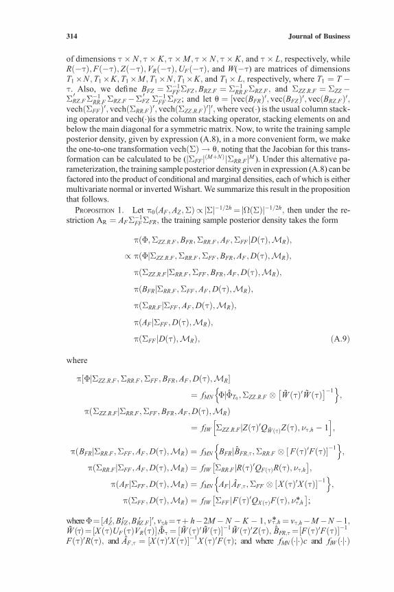
FFSFZ ; and let u ¼ ½vecðBFRÞ0; vecðBFZÞ0; vecðBRZ:FÞ0;vechðSFFÞ0; vechðSRR:FÞ0; vechðSZZ:R:FÞ0�0;where vec(�) is the usual column stack-ing operator and vech(�)is the column stacking operator, stacking elements on andbelow the main diagonal for a symmetric matrix. Now, to write the training sampleposterior density, given by expression (A.8), in a more convenient form, we makethe one-to-one transformation vechðSÞ ! u; noting that the Jacobian for this trans-formation can be calculated to be (jSFFjðMþNÞjSRR:FjM ). Under this alternative pa-rameterization, the training sample posterior density given in expression (A.8) can befactored into the product of conditional and marginal densities, each of which is eithermultivariate normal or invertedWishart. We summarize this result in the propositionthat follows.

Proposition 1. Let p0ðAF ;AZ ;SÞ / jSj�1=2h ¼jWðSÞj�1=2h; then under the re-striction AR ¼ AFS�1

FFSFR; the training sample posterior density takes the form

pðF;SZZ:R:F ;BFR;SRR:F ;AF ;SFFjDðtÞ;MRÞ;

/ pðFjSZZ:R:F ;SRR:F ;SFF ;BFR;AF ;DðtÞ;MRÞ;

pðSZZ:R:FjSRR:F ;SFF ;BFR;AF ;DðtÞ;MRÞ;

pðBFRjSRR:F ;SFF ;AF ;DðtÞ;MRÞ;

pðSRR:FjSFF ;AF ;DðtÞ;MRÞ;

pðAFjSFF ;DðtÞ;MRÞ;

pðSFF jDðtÞ;MRÞ; ðA:9Þ

where

p FjSZZ:R:F ;SRR:F ;SFF ;BFR;AF ;DðtÞ;MR½ �

¼ fMN FjFT0 ;SZZ:R:F � W ðtÞ0W ðtÞ� ��1

n o;

p SZZ:R:FjSRR:F ;SFF ;BFR;AF ;DðtÞ;MRð Þ

¼ fIW SZZ:R:FjZðtÞ0QW ðtÞZðtÞ; �t;h � 1h i

;

p BFRjSRR:F ;SFF ;AF ;DðtÞ;MRð Þ ¼ fMN BFRjBFR;t;SRR:F � FðtÞ0FðtÞ½ ��1n o

;

p SRR:FjSFF ;AF ;DðtÞ;MRð Þ ¼ fIW SRR:FjRðtÞ0QFðtÞRðtÞ; �t;h� �

;

p AFjSFF ;DðtÞ;MRð Þ ¼ fMN AFjAF;t;SFF � X ðtÞ0X ðtÞ½ ��1n o

;

pðSFF ;DðtÞ;MRÞ ¼ fIW SFFjFðtÞ0QX ðtÞFðtÞ; �t;h*� �

;

whereF¼½AZ0;BFZ

0 ;BRZ:F0 �0; vt;h¼tþ h�2M� N � K � 1; vt;h* ¼ vt;h�M�N�1;

W ðtÞ¼½X ðtÞUFðtÞVRðtÞ�;Ft ¼ ½W ðtÞ0W ðtÞ��1W ðtÞ0ZðtÞ; BFR;t¼½FðtÞ0FðtÞ��1

FðtÞ0RðtÞ; and AF;t ¼ ½X ðtÞ0X ðtÞ��1X ðtÞ0FðtÞ; and where fMN ð�j�Þc and fIW ð�j�Þ


denote, respectively, the probability density function of a matrix-normal distributionand that of an inverted Wishart distribution.

Proof. To begin, note that on making the transformation vechðSÞ ! u; whereu ¼ ½vecðBFRÞ0; vecðBFZÞ0; vecðBRZ:FÞ0; vechðSFFÞ0; vechðSRR:FÞ0; vechðSZZ:R:FÞ0�0;the density of the diffuse-prior posterior distribution based on the training sample canbe written as

pðF;SZZ:R:F;BFR;SRR:F ;AF ;SFFjDðtÞ;MRÞ /ð2pÞ�12tðMþNþKÞjSFFj�

12ðtþh�2M�2NÞ

jSRR:Fj�12ðrþh�2MÞjSZZ:R:Fj�

12t exp � 1

2Tr WðuÞ�1


; ðA:10Þ

where V ðtÞ ¼ ½VRðtÞUFðtÞUZðtÞ� and VRðtÞ;UFðtÞ; andUZðtÞ are matrices madeup of the first t rows of the partitioned error matrices VR ¼ ½VRðtÞ0;VRð�tÞ0�0;UF ¼ ½UFðtÞ0;UFð�tÞ0�0; and UZ ¼ ½UZðtÞ0;UZð�tÞ0�0; and where WðuÞ�1 de-notes the inverse of the error covariance matrix W(S) but expressed as a function ofthe new parameterization u. Moreover, applying the formula for the inverse of a 3�3matrix partition, we can write WðuÞ�1

in explicit form as follows:

WðuÞ�1 ¼W11 W12 W13

W21 W22 W23

W31 W32 W33

0B@

1CA; ðA:11Þ

where W11 ¼ S�1RR:F þ BRZ:FS�1

ZZ:R:FB0

RZ:F ;W12 ¼ BRZ:FS�1

ZZ:R:FBFZ ;W22 ¼ S�1FF þ

BFZS�1ZZ:R:FBFZ ;W 13 ¼ �BRZ:FS�1

ZZ:R:F;W23 ¼ �BFZS�1

ZZ:R:F ; andW33 ¼ S�1

ZZ:R:F andwhere W21 ¼ W120 ;W31 ¼ W130 ; and W32 ¼ W230 . It follows from (A.10) that thetraining sample posterior density depends on the parameters AF ;AZ ;BFR;BFZ ;and BRZ:F through the relationships VRðtÞ ¼ RðtÞ � FðtÞBFR;UFðtÞ ¼ FðtÞ �X ðtÞAF ; and UZðtÞ ¼ ZðtÞ � X ðtÞAZ and through the matrix function WðuÞ�1

.

Next, making use of expression (A.11) and some straightforward algebra, it is easyto show that the trace expression in the exponential term of equation (A.10) can berewritten as follows:

Tr½WðuÞ�1V ðtÞ0V ðtÞ� ¼ Tr

S�1

FF

�FðtÞ0QX ðtÞFðtÞ

þ AF � AF;t �0

X ðtÞ0X ðtÞ AF � AF;t ��

þ Tr S�1RR:FRðtÞ0QFðtÞRðtÞ þ BFR � BFR;t

�0FðtÞ0FðtÞ BFR � BFR;t

�� þ Tr S�1

ZZ:R:F ZðtÞ0QW ðtÞZðtÞ þ F� Ft �0

W ðtÞ0W ðtÞ F� Ft �h in o

; ðA:12Þ

whereAF;t; BF;t; Ft;FðtÞ;RðtÞ; and Z(t) are as previously defined.

Now, note that W ðtÞ ¼ W ðtÞH ; where W ðtÞ ¼ ½X ðtÞFðtÞRðtÞ� and

H ¼IMþ1 �AF 0

0 IK �BFR

0 0 IN

264

375; ðA:13Þ


and it is obvious that jH j ¼ 1; so H is nonsingular. It follows that, for each value ofBFR and AF ; we have that ZðtÞ0QW ðtÞZðtÞ ¼ ZðtÞ0QW ðtÞZðtÞ and jW ðtÞ0W ðtÞj ¼jW ðtÞ0W ðtÞj; so that, in particular, neither ZðtÞ0QW ðtÞZðtÞ nor jW ðtÞ0W ðtÞj de-pends on the unknown parametersAF andBR. Using these facts, we can factor (A.10)into a product of (unnormalized) conditional and marginal probability density func-tions, each of which is either the density of a matrix-variate normal distribution or thatof an inverted Wishart distribution. Hence, on appropriate renormalization, we obtainthe training sample posterior density given by expression (A.9). Q.E.D.

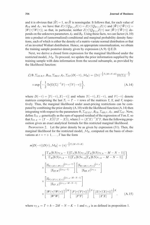
Next, we derive a closed form expression for the marginal likelihood under therestricted model,MR. To proceed, we update the prior information supplied by thetraining sample with data information from the second subsample, as provided bythe likelihood function:

LðF;SZZ:R:F ;BFR;SRR:F;AF ;SFFjDð�tÞ;MRÞ ¼ ð2pÞ�12T1ðMþNþKÞjWðSÞj�

T12

�exp � 1

2Tr½WðSÞ�1

V ð�tÞ0V ð�tÞ��

; ðA:14Þ

where Dð�tÞ ¼ ½Y ð�tÞ;X ð�tÞ� and where Y ð�tÞ;X ð�tÞ; and V ð�tÞ denotematrices comprising the last T1 ¼ T � t rows of the matrices Y, X, and V, respec-tively. Thus, the marginal likelihood under asset-pricing restrictions can be com-puted by combining the prior density (A.10) with the likelihood function (A.14) thenintegrating with respect to the parametersF,SZZ:R:F ;BFR;SRR:F ;AF ; andSFF . Now,define SYY :X generically as the sum of squared residual of the regression of Yon X, sothat SYY :X ¼ ðY � X bÞ0ðY � X bÞ;where b ¼ ðX 0X Þ�1

X 0Y ; then the following prop-osition gives an exact analytical formula for this restricted marginal likelihood.

Proposition 2. Let the prior density be as given by expression (31). Then, themarginal likelihood for the restricted model, MR; computed on the basis of obser-vations at t ¼ tþ 1; . . . ; T has the form

m½Dð�tÞjDðtÞ;MR� ¼ ðpÞ�12T1ðMþNþKÞ

� GM ½0:5ðvT ;h � 1Þ�GN ½0:5ðvT ;hÞ�GK ½0:5ðvT ;h �M � N � 1Þ�GM ½0:5ðvt;h � 1Þ�GN ½0:5vt;h�GK ½0:5ðvt;h �M � N � 1Þ�

� �

�jSZðtÞZðtÞ:W ðtÞj

12ð�t; h�1Þ

jSZZ:W j12ð�T ;h�1Þ

" #jSRðtÞRðtÞ:FðtÞj

12�t; h

jSRR :Fj12� T ; h

" #

�jSFðtÞFðtÞ:X ðtÞj

12ð�t; h�M�N�1Þ

jSFF:X j12ð�T ; h�M�N�1Þ

" #

� jW ðtÞ0W ðtÞjjW 0W j

�12M jFðtÞ0FðtÞj

jF 0Fj

�12N jX ðtÞ0X ðtÞj

jX 0X j

�12K

; ðA:15Þ

where vT ;h ¼ T þ h� 2M � N � K � 1 and vt;h is as defined in proposition 1.


Proof. Set T1 ¼ T� t and note that the likelihood function for the second partof the sample, as given by expression (A.14), can be factored as follows:

LðF;SZZ:R:F ;BFR;SRR:F;AF ;SFFjDð�tÞ;MRÞ ¼ ð2pÞ�12T1ðNþMþKÞjSRR:Fj�

12T1

exp

�� 1

2TrnS�1

RR:F

hSRð�tÞRð�tÞ:Fð�tÞ þðBFR� BFR;tÞ0Fð�tÞ0Fð�tÞðBFR� BFR;tÞ

io�

jSZZ:R:Fj�12T1 exp

�� 1

2TrnS�1

ZZ:R:F

hSZð�tÞZð�tÞ:W ð�tÞ

þ ðF� FT1Þ0W ð�tÞ0W ð�tÞðF� FT1Þio�

jSFFj�12T1 exp

�� 1

2TrnS�1

FF

hSFð�tÞFð�eÞ:X ð�tÞ

þ ðAF � AF;tÞ0X ð�tÞ0X ð�tÞðAF � AF;tÞio�

; ðA:16Þ

and where FT1¼ ½W ð�tÞ0W ð�tÞ��1W ð�tÞ0Zð�tÞ; BFR;T1 ¼ ½Fð�tÞ0Fð�tÞ��1�

Fð�tÞ0Rð�tÞ;AF;T1 ¼ ½X ð�tÞ0X ð�tÞ��1X ð�tÞ0Fð�tÞ; and W ð�tÞ ¼ ½X ð�tÞ;VR ð�tÞ;UFð�tÞ�.

Next, observe that, for each value of BFR and AF ; the following relationships hold:Z 0QWZ ¼ Z 0QWZ and jW ðtÞ0W ðtÞ þ W ð�tÞ0W ð�tÞ j¼ j W 0W j;where thematrixH is as defined in expression (A.13). Thus, neither Z 0QWZ nor jW 0W j depends on theunknown parameters AF and BFR. Making use of these facts, we can construct thejoint posterior density of F;SZZ:R:F ;BFR;SRR:F ;AF ; and SFF given the data by com-bining the likelihood function (A.16) with the prior density given in expression (A.9).The marginal likelihood given in expression (A.15) then can be obtained straight-forwardly by integrating this joint posterior density with respect to the param-eters F;SZZ:R:F ;BFR;SRR:F ;AF ; and SFF over their respective support.

Computing the Marginal Likelihood for the Unrestricted Model

Our point of departure is the linear system given by (A.1)–(A.3). Observe that, in theunrestricted case, we can rewrite equation (A.1) as

R ¼ X ðAR � AFBFRÞ þ FBFR þ VR; ðA:17Þ

where BFR ¼ S�1FFSFR and VR ¼ UR � UFS�1

FFSFR. Note, of course, that equa-tion (A.4) of the last subsection is nested within the more general equation givenby (A.17) here. Now, to specify a prior based on the training sample posterior dis-tribution, we start again with the diffuse prior p0ðAR;AF ;AZ ;SÞ/ jSj�1=2h ¼jWðSÞj�1=2h; with WðSÞ as defined in expression (A.7), and use the first t obser-vations as a training sample.


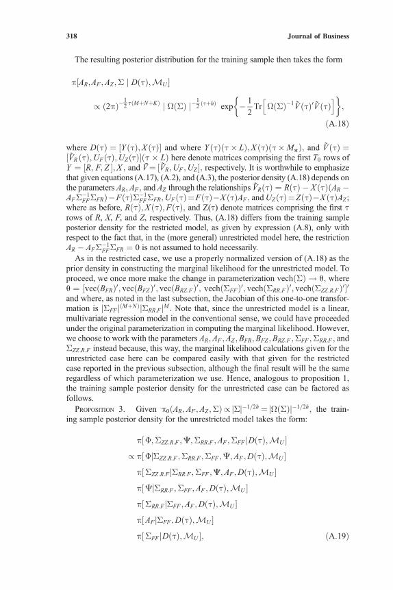
The resulting posterior distribution for the training sample then takes the form

p½AR;AF ;AZ ;S j DðtÞ;MU �

/ ð2pÞ�12tðMþNþKÞ j WðSÞ j�

12ðtþhÞ exp � 1

2Tr WðSÞ�1


;

ðA:18Þ

where DðtÞ ¼ ½Y ðtÞ;X ðtÞ� and where Y ðtÞðt� LÞ;X ðtÞðt�M*Þ; and V ðtÞ ¼

½VR ðtÞ;UFðtÞ;UZðtÞ�ðt � LÞ here denote matrices comprising the first T0 rows ofY ¼ ½R; F; Z �;X ; and V¼ ½VR;UF ;UZ �; respectively. It is worthwhile to emphasizethat given equations (A.17), (A.2), and (A.3), the posterior density (A.18) depends onthe parameters AR;AF ; and AZ through the relationships VRðtÞ ¼ RðtÞ � X ðtÞðAR �AFS�1

FFSFRÞ�FðtÞS�1FFSFR;UFðtÞ¼FðtÞ�X ðtÞAF ; andUZðtÞ¼ZðtÞ�X ðtÞAZ ;

where as before, RðtÞ;X ðtÞ;FðtÞ; and Z(t) denote matrices comprising the first trows of R, X, F, and Z, respectively. Thus, (A.18) differs from the training sampleposterior density for the restricted model, as given by expression (A.8), only withrespect to the fact that, in the (more general) unrestricted model here, the restrictionAR � AFS�1

FFSFR ¼ 0 is not assumed to hold necessarily.

As in the restricted case, we use a properly normalized version of (A.18) as theprior density in constructing the marginal likelihood for the unrestricted model. Toproceed, we once more make the change in parameterization vechðSÞ ! u; whereu ¼ ½vecðBFRÞ0; vecðBFZÞ0; vecðBRZ:FÞ0; vechðSFFÞ0; vechðSRR:FÞ0; vechðSZZ:R:FÞ0�0and where, as noted in the last subsection, the Jacobian of this one-to-one transfor-mation is jSFFjðMþNÞjSRR:FjM . Note that, since the unrestricted model is a linear,multivariate regression model in the conventional sense, we could have proceededunder the original parameterization in computing the marginal likelihood. However,we choose to work with the parameters AR;AF ;AZ ;BFR;BFZ ;BRZ:F ;SFF ;SRR:F ; andSZZ:R:F instead because, this way, the marginal likelihood calculations given for theunrestricted case here can be compared easily with that given for the restrictedcase reported in the previous subsection, although the final result will be the sameregardless of which parameterization we use. Hence, analogous to proposition 1,the training sample posterior density for the unrestricted case can be factored asfollows.

Proposition 3. Given p0ðAR;AF ;AZ ;SÞ / jSj�1=2h ¼jWðSÞj�1=2h; the train-ing sample posterior density for the unrestricted model takes the form:

p F;SZZ:R:F ;C;SRR:F ;AF ;SFFjDðtÞ;MU½ �

/ p FjSZZ:R:F ;SRR:F ;SFF ;C;AF ;DðtÞ;MU½ �

p SZZ:R:FjSRR:F ;SFF ;C;AF ;DðtÞ;MU½ �

p CjSRR:F ;SFF ;AF ;DðtÞ;MU½ �

p SRR:FjSFF ;AF ;DðtÞ;MU½ �

p AFjSFF ;DðtÞ;MU½ �

p SFFjDðtÞ;MU½ �; ðA:19Þ


where C ¼ ½AR0BFR

0 �0;F ¼ ½AZ0BFZ

0 BRZ:F0 �0; and

p FjSZZ:R:F ;SRR:F ;SFF ;C;AF ;DðtÞ;SFFjDðtÞ;MU½ �

¼ fMN FjFt;SZZ:R:F � W ðtÞ0W ðtÞ� ��1

n op SZZ:R:FjSRR:F ;SFF ;C;AF ;DðtÞ;SFF jDðtÞ;MU½ �

¼ fIW SZZ:R:FjZðtÞ0QW ðtÞZðtÞ; �t;h � 1h i

;

p CjSRR:F ;SFF ;AF ;DðtÞ;SFF jDðtÞ;MU½ �

¼ fMN CjCt;SRR:F � W ðtÞð1Þ0W ðtÞð1Þh i�1

� �p SRR:FjSFF ;AF ;DðtÞ;SFFjDðtÞ;MU½ �

¼ fIW SRR:FjR 00QW ð1ÞðtÞR0; �t;h �M � 1

h i;

p AFjSFF ;DðtÞ;SFFjDðtÞ;MUð Þ ¼ fMN AFjAF;t;SFF � X ðtÞ0X ðtÞ½ ��1n o

;

p SFFjDðtÞ;SFFjDðtÞ;MUð Þ ¼ fIW SFFjFðtÞ0QX ðtÞFðtÞ; �t;h*� �

;

where W ðtÞ ¼ ½X ðtÞ;UFðtÞ; VRðtÞ�; Ft ¼ ½W ðtÞ0W ðtÞ��1W ðtÞ0ZðtÞ; vt;h* ¼ vt;h �M � N � 1; Ct ¼ ½W ðtÞð1Þ0W ðtÞð1Þ��1

W ðtÞð1Þ0RðtÞ; and AF;t ¼ ½X ðtÞ0X ðtÞ��1�½X ðtÞ0FðtÞ.

Proof. Note that, on making the transformation vechðSÞ!u; where u ¼½vecðBFRÞ0; vecðBFZÞ0; vecðBRZ:FÞ0; vechðSFFÞ0; vechðSRR:FÞ0; vechðSZZ:R:FÞ0�0; thedensity of the diffuse-prior posterior distribution based on the training samplecan be written as

pðF;SZZ:R:F ;C;SRR:F ;AF ;SFFjDðtÞ;MU Þ / ð2pÞ�12tðMþNþKÞ

� jSFF j�12ðtþh�2M�2NÞjSRR:Fj�

12ðtþh�2MÞjSZZ:R:Fj�

12T0

� exp � 1

2Tr WðuÞ�1


; ðA:20Þ

where WðuÞ�1is as defined in expression (A.11) and where V ðtÞ ¼ ½VRðtÞ;UFðtÞ;

UZðtÞ�. The posterior density (A.20), thus, depends on the parameters AR;AF ;AZ

BFR;BFZ ; andBRZ:F through the relationships VRðtÞ ¼ RðtÞ � X ðtÞðAR � AFBFRÞ�FðtÞ;UFðtÞ ¼ FðtÞ� X ðtÞAF ; and UZðtÞ ¼ ZðtÞ� X ðtÞAZ and through the ma-trix function WðuÞ�1. Now, similar to the proof of proposition 1, one can show bystraightforward calculation that the trace expression in the exponential componentof (A.20) can be written in the form

Tr WðuÞ�1V ðtÞ0V ðtÞ

h i¼ Tr

nS�1

FF

hFðtÞ0QX ðtÞFðtÞ

þ AF � AF;t �0X ðtÞ0X ðtÞ AF � AF;t

�ioþ Tr S�1

RR:F RðtÞ0QW ðtÞð1ÞRðtÞ þ C� Ct

� �0W ðtÞð1Þ0W ðtÞð1Þ C� Ct

� �h in oþ Tr S�1

ZZ:R:F ZðtÞ0QW ðtÞZðtÞ þ F� Ft �0W ðtÞ0W ðtÞ F� Ft

�h in o; ðA:21Þ


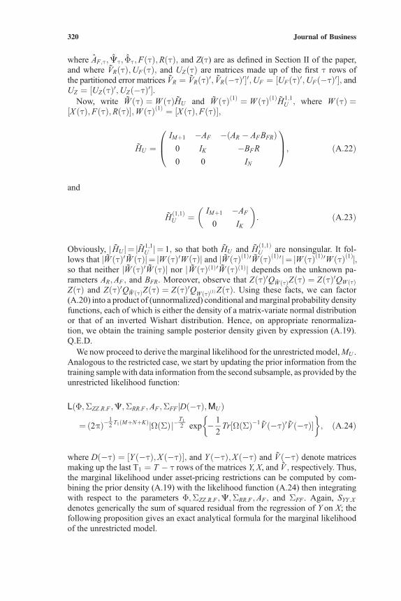
where AF;t; Ct; Ft;FðtÞ;RðtÞ; and Z(t) are as defined in Section II of the paper,and where VRðtÞ;UFðtÞ; and UZðtÞ are matrices made up of the first t rows ofthe partitioned error matrices VR ¼ VRðtÞ0; VRð�tÞ0�0;UF ¼ ½UFðtÞ0;UFð�tÞ0�; andUZ ¼ ½UZðtÞ0;UZð�tÞ0�.

Now, write W ðtÞ ¼ W ðtÞHU and W ðtÞð1Þ ¼ W ðtÞð1ÞH1;1U ; where W ðtÞ ¼

½X ðtÞ;FðtÞ;RðtÞ�;W ðtÞð1Þ ¼ ½X ðtÞ;FðtÞ�;

HU ¼IMþ1 �AF �ðAR � AFBFRÞ0 IK �BFR

0 0 IN

0B@

1CA; ðA:22Þ

and

Hð1;1ÞU ¼

IMþ1 �AF

0 IK

� �: ðA:23Þ

Obviously, | HU j¼ jH1;1U j¼ 1; so that both HU and H

ð1;1ÞU are nonsingular. It fol-

lows that jW ðtÞ0W ðtÞj¼ jW ðtÞ0W ðtÞj and jW ðtÞð1Þ0W ðtÞð1Þ0 j¼ jW ðtÞð1Þ0W ðtÞð1Þj;so that neither jW ðtÞ0W ðtÞj nor jW ðtÞð1Þ0W ðtÞð1Þj depends on the unknown pa-rameters AR;AF ; and BFR. Moreover, observe that ZðtÞ0QW ðtÞZðtÞ ¼ ZðtÞ0QW ðtÞZðtÞ and ZðtÞ0QW ðtÞZðtÞ ¼ ZðtÞ0Q

W ðtÞð1ÞZðtÞ. Using these facts, we can factor(A.20) into a product of (unnormalized) conditional andmarginal probability densityfunctions, each of which is either the density of a matrix-variate normal distributionor that of an inverted Wishart distribution. Hence, on appropriate renormaliza-tion, we obtain the training sample posterior density given by expression (A.19).Q.E.D.

We now proceed to derive the marginal likelihood for the unrestricted model,MU .Analogous to the restricted case, we start by updating the prior information from thetraining sample with data information from the second subsample, as provided by theunrestricted likelihood function:

LðF;SZZ:R:F ;C;SRR:F ;AF ;SFF jDð�tÞ;MU Þ

¼ ð2pÞ�12T1ðMþNþKÞjWðSÞj�

T12 exp � 1

2Tr½WðSÞ�1

V ð�tÞ0V ð�tÞ��

; ðA:24Þ

where Dð�tÞ ¼ ½Y ð�tÞ;X ð�tÞ�; and Y ð�tÞ;X ð�tÞ and V ð�tÞ denote matricesmaking up the last T1 ¼ T � t rows of the matrices Y, X, and V ; respectively. Thus,the marginal likelihood under asset-pricing restrictions can be computed by com-bining the prior density (A.19) with the likelihood function (A.24) then integratingwith respect to the parameters F;SZZ:R:F ;C;SRR:F ;AF ; and SFF . Again, SYY :Xdenotes generically the sum of squared residual from the regression of Y on X; thefollowing proposition gives an exact analytical formula for the marginal likelihoodof the unrestricted model.


Proposition 4. Let the prior density be as given by expression (A.19). Then, themarginal likelihood for the unrestricted model, MU ; computed on the basis of ob-servations at t ¼ tþ 1; . . . ; T has the form

m½Dð�tÞjDðtÞ;MU � ¼ ðpÞ�12T1ðMþNþKÞ

� GM ½0:5ðvT ;h � 1Þ�GN ½0:5ðvT ;h �M � 1Þ�GK ½0:5ðvT ;h �M � N � 1Þ�GM ½0:5ðvt;h � 1Þ�GN ½0:5ðvt;h �M � 1Þ�GK ½0:5ðvt;h �M � N � 1Þ�

� �

�jSZðtÞZðtÞ:W ðtÞj

12ð�t; h�1Þ

jSZZ:W j12ð�T ; h�1Þ

" #jS

RðtÞRðtÞ:W ðtÞð1Þ j12ð�t; h�M�1Þ

jSRR:W ð1Þ j12ð�T ; h�M�1Þ

" #

�jSFðtÞFðtÞ:X ðtÞj

12ð�t; h�M�N�1Þ

jSFF:X j12ð�T ; h�M�N�1Þ

" #

� jW ðtÞ0W ðtÞjjW 0W j

�12M jW ðtÞð1Þ0W ðtÞð1Þj

jW ð1Þ0W ð1Þj

" #12N

jX ðtÞ0X ðtÞjjX 0X j

�12K

; ðA:25Þ

where, as before, vt;h ¼ tþ h� 2M � N � K �1 and vT ;h ¼ T þ h� 2M � N �K � 1.

Proof. Note first that the unrestricted likelihood for the primary sample can befactored as follows:

L F;SZZ:R:F ;C;SRR:F ;AF ;SFFjDð�tÞ;MU½ � ¼ ð2pÞ�12T1ðMþNþKÞjSZZ:R:Fj�

12T1

ðA:26Þ

exp

�� 1

2TrnS�1

ZZ:R:F

hZð�tÞ0QW ð�tÞZð�tÞ

þ F� FT1

�0W ð�tÞ0W ð�tÞ F� FT1

�io��jSRR:Fj�

12T1

� exp

�� 1

2TrnS�1

RR:F

hRð�tÞ0Q

W ð�tÞð1ÞRð�tÞ

þ C� CT1

� �0W ð�tÞð1Þ0W ð�tÞð1Þ C� CT1

� �io��jSFF j�

12T1

� exp

�� 1

2TrnS�1

FF

hFð�tÞ0QX ð�tÞFð�tÞ

þ AF � AF;T1

�0X ð�tÞ0X ð�tÞ AF � AF;T1

�io�;

where FT1 ¼ ½W ð�tÞ0W ð�tÞ��1W ð�tÞ0Zð�tÞ; CT1 ¼ ½W ð�tÞð1Þ0W ð�tÞð1Þ��1

W ð�tÞð1Þ0Rð�tÞ; AF;T1 ¼ ½X ð�tÞ0X ð�tÞ��1X ð�tÞ0Fð�tÞ; and W ð�tÞ ¼ ½X ð�tÞ;

UFð�tÞ; VRð�tÞ�.Next, observe that, for each value of AR;AF ; and BFR; the following relationships

hold: Z 0QWZ ¼ Z 0QWZ;R0QW ð1ÞR¼R0QW ð1ÞR; jW 0W j¼ jW 0W j; and jW ð1Þ0W ð1Þj ¼jW ð1Þ0W ð1Þj; where the matrix HU and HU

ð1;1Þ are as defined in expressions (A.22)


and (A.23). It follows that, conditioned on the data, the expressions Z 0QWZ;R0QW ð1ÞR; jW 0W j; and jW ð1Þ0W ð1Þj do not depend on the unknown parametersAR;AF ;and BFR. Making use of these facts, we can construct the joint posterior density ofF;SZZ:R:F ;BFR;SRR:F ;AF ; and SFF given the data by combining the likelihoodfunction for the unrestricted model, expression (A.26) with the prior density given inexpression (A.19). The marginal likelihood for the unrestricted model as given byexpression (A.25) can then be obtained in a straightforward manner by integratingthis joint posterior density with respect to the parameters F;SZZ:R:F ;BFR;SRR:F ;AF ;and SFF over their respective support. Q.E.D.

References

Ahn, S. C., and C. Gadarowski. 1999. Small sample properties of the model specificationtest based on the Hansen-Jagannathan distance. Working paper, Arizona State University.

Avramov, D. 2002. Stock return predictability and model uncertainty. Journal of FinancialEconomics 64:423–58.

———. 2004. Stock return predictability and asset pricing models. Review of FinancialStudies 17:699–738.

Berger, J. O., and L. R. Pericchi. 1996. The intrinsic Bayes factor for model selection andprediction. Journal of the American Statistical Association 91:109–22.

Black, F., M. Jensen, and M. Scholes. 1972. The capital asset pricing model: Some empiricaltests. In Studies in the theory of capital markets, ed. M. C. Jensen. New York: Praeger.

Breeden, D. T. 1979. An intertemporal asset pricing model with stochastic consumption andinvestment opportunities. Journal of Financial Economics 7:265–296.

Breeden, D. T., M. Gibbons, and R. Litzenberger. 1989. Empirical tests of the consumptionoriented CAPM. Journal of Finance 44:231–62.

Campbell, J. 1987. Stock returns and the term structure. Journal of Financial Economics18:373–99.

———. 1996. Understanding risk and return. Journal of Political Economy 104:572–621.Cochrane, J. H. 1996. A cross-sectional test of an investment-based asset pricing model.

Journal of Political Economy 104:572–621.DeBondt, W., and R. Thaler. 1985. Does the stock market overreact? Journal of Finance

40:793–805.Dumas, B., and B. Solnik. 1995. The world price of foreign exchange risk. Journal of

Finance 50:445–79.Fama, E. F., and K. R. French. 1993. Common risk factors in the returns on stocks and

bonds. Journal of Financial Economics 33:3–56.———. 1996. Multifactor explanations of asset pricing anomalies. Journal of Finance 51:

55–84.———. 1998. Value versus growth: The international evidence. Journal of Finance 53:

1975–99.Fama, E. F., and J. D. MacBeth. 1973. Risk, return, and equilibrium: Empirical tests.

Journal of Political Economy 81:607–36.Ferson, W., and S. R. Forester. 1994. Finite sample properties of the generalized method of

moments in tests of conditional asset pricing models. Journal of Financial Economics36:29–56.

Geweke, J., and G. Zhou. 1996. Measuring the pricing errors of the arbitrage pricing theory.Review of Financial Studies 9:557–87.

Gibbons, M. R., S. A. Ross, and J. Shanken. 1989. A test of the efficiency of a givenportfolio. Econometrica 57:1121–52.

Ghysels, E. 1998. On stable factor structures in the pricing of risk: Do time-varying betashelp or hurt? Journal of Finance 53:549–73.

Hansen, L. P. 1982. Large sample properties of generalized method of moments estimators.Econometrica 50:1029–054.

Hansen, L. P., and R. Jagannathan. 1997. Assessing specification errors in stochastic dis-count factor models. Journal of Finance 52:557–90.


Hansen, L. P., and S. F. Richard. 1987. The role of conditioning information in deducingtestable. Econometrica 55:587–613.

Harvey, C. 1991. The world price of covariance risk. Journal of Finance 46:111–57.Harvey, C., and G. Zhou. 1990. Bayesian inference in asset pricing tests. Journal of Financial

Economics 26:221–54.Haugen, R. 1995. The new finance: The case against efficient markets. Englewood Cliffs, N.:

Prentice-Hall.Huberman, G., and S. Kandel. 1987.Mean variance spanning. Journal of Finance 42:873–88.Jeffreys, H. 1961. Theory of probability. New York: Oxford University Press.Kan, R., and G. Zhou. 1999. A critique of the stochastic discount factor methodology.

Journal of Finance 54:1221–48.———. 2003. Modeling non-normality using multivariate t: Implications for asset pricing.

Working paper, Washington University.Kass, R. E., and A. E. Raftery. 1995. Bayes factors. Journal of the American Statistical

Association 90:773–95.Kandel, S., R. McCulloch, and R. Stambaugh. 1995. Bayesian inference and portfolio

efficiency. Review of Financial Studies 8:1–53.Korajczyk, R. A., and C. J. Viallet. 1989. An empirical investigation of international asset

pricing. Review of Financial Studies 4:553–85.Lakonishok, J., A. Shleifer, and R. Vishny. 1994. Contrarian investment, extrapolation, and

risk. Journal of Finance 49:1541–78.Lettau, M., and S. Ludvigson. 2001. Resurrecting the (C)CAPM: A cross sectional test when

risk premia are time-varying. Journal of Political Economy 109:1238–87.Lintner, J. 1965. Security prices, risk, and maximal gains from diversification. Journal of

Finance 20:587–615.McCulloch, R., and P. E. Rossi. 1991. A Bayesian approach to testing the arbitrage pricing

theory. Journal of Econometrics 49: 141–168.Phillips, P. C. B., and W. Ploberger. 1996. An asymptotic theory of Bayesian inference for

time series. Econometrica 64:381–412.Roll, R. 1977. A critique of the asset pricing theory’s tests. Part I. On past and potential

testability of the theory. Journal of Financial Economics 4:129–76.Shanken, J. 1987. A Bayesian approach to testing portfolio efficiency. Journal of Financial

Economics 19:217–44.Sharpe, W. F. 1964. Capital asset prices: A theory of market equilibrium under conditions of

risk. Journal of Finance 19:425–42.Sims, C. A. 1988. Bayesian skepticism on unit root econometrics. Journal of Economic

Dynamics and Control 12:463–74.Sims, C. A., and H. Uhlig. 1991. Understanding unit root: A helicopter tour. Econometrica

59:1591–99.Solnik, B. 1974. An equilibrium model of the international capital market. Journal of

Economic Theory 8:500–24.Tu, J., and G. Zhou. 2004. Data-generating process uncertainty: What difference does it

make in portfolio decisions? Journal of Financial Economics 72:385–421.Zellner, A. 1971. An introduction to Bayesian inference in econometrics. New York: John

Wiley and Sons.


An Exact Bayes Test of Asset Pricing Models with ...pluto.huji.ac.il/~davramov/paper3.pdf · An...

Documents

Transcript of An Exact Bayes Test of Asset Pricing Models with ...pluto.huji.ac.il/~davramov/paper3.pdf · An...