An Evaluation of the Performance of Applied General Equilibrium Models of

the Impact of NAFTA

Timothy J. Kehoe University of Minnesota

and Federal Reserve Bank of Minneapolis

September 2003

www.econ.umn.edu/~tkehoe

Evaluate the performances of three of the most prominent multisectoral static applied general equilibrium models used to predict the impact of the North American Free Trade Agreement. Findings:

• Models drastically underestimated the impact of NAFTA on trade.

• Models failed to capture much of the relative impacts on different sectors.

Suggestions for future work:

• Develop mechanisms that generate large increases in trade in product categories with little or no previous trade.

• Explain changes in productivity.

What Went Wrong in Modeling the Impact of the North American Free Trade Agreement?

Applied general equilibrium models were the only analytical game in town when it came to analyzing the impact of NAFTA in 1992-1993. Typical sort of model: Static applied general equilibrium model with large number of industries and imperfect competition (Dixit-Stiglitz or Eastman-Stykolt) and finite number of firms in some industries. In some numerical experiments, new capital is placed in Mexico owned by consumers in the rest of North America to account for capital flows. Examples: Brown-Deardorff-Stern model of Canada, Mexico, and the United States Cox-Harris model of Canada Sobarzo model of Mexico

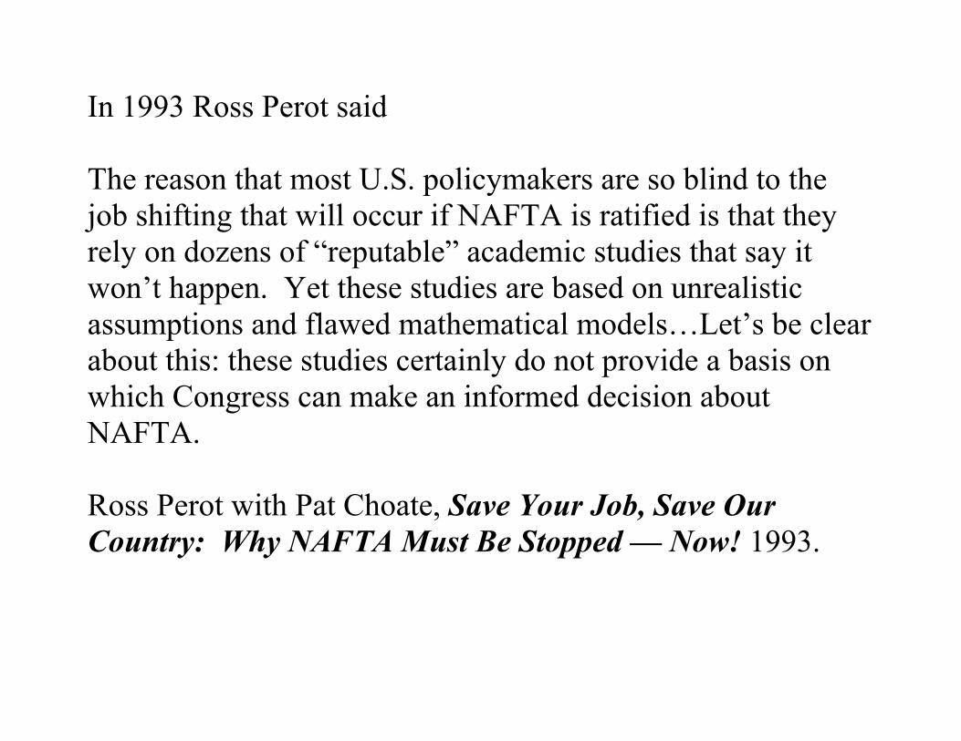
In 1993 Ross Perot said The reason that most U.S. policymakers are so blind to the job shifting that will occur if NAFTA is ratified is that they rely on dozens of “reputable” academic studies that say it won’t happen. Yet these studies are based on unrealistic assumptions and flawed mathematical models…Let’s be clear about this: these studies certainly do not provide a basis on which Congress can make an informed decision about NAFTA. Ross Perot with Pat Choate, Save Your Job, Save Our Country: Why NAFTA Must Be Stopped — Now! 1993.

In his comments, Timothy J. Kehoe observes that investment flows have generated a sharp increase in Mexican investment, GDP, and trade deficits. Policy makers have become concerned about the sustainability of this behavior, an issue not addressed by the CGE models. Kehoe also stresses that CGE remains at an early stage of development. He emphasizes the need for ex-post verification to achieve validation of these models. Kehoe also argues for more work on the impact of NAFTA on the behavior of financial intermediaries, policy credibility, demographic structures, and total factor productivity growth. Nora Lustig, Barry P. Bosworth, and Robert Z. Lawrence, editors, North American Free Trade: Assessing the Impact, 1992.

Research Agenda: • Compare results of numerical experiments of models with

data. • Determine what shocks — besides NAFTA policies — were

important. • Construct a simple applied general equilibrium model and

perform experiments with alternative specifications to determine what was wrong with the 1992-1993 models.

Applied GE Models Can Do a Good Job!

Spain: Kehoe-Polo-Sancho (1992) evaluation of the performance of the Kehoe-Manresa-Noyola-Polo-Sancho-Serra MEGA model of the Spanish economy: A Shoven-Whalley type model with perfect competition, modified to allow government and trade deficits and unemployment (Kehoe-Serra). Spain’s entry into the European Community in 1986 was accompanied by a fiscal reform that introduced a value-added tax (VAT) on consumption to replace a complex range of indirect taxes, including a turnover tax applied at every stage of the production process. What would happen to tax revenues? Trade reform was of secondary importance.

Canada-U.S.: Fox (1999) evaluation of the performance of the Brown-Stern (1989) model of the 1989 Canada-U.S. FTA.

Other changes besides policy changes are important!

Changes in Consumer Prices in the Spanish Model (Percent)

data model model model sector 1985-1986 policy only shocks only policy&shocks food and nonalcoholic beverages 1.8 -2.3 4.0 1.7 tobacco and alcoholic beverages 3.9 2.5 3.1 5.8 clothing 2.1 5.6 0.9 6.6 housing -3.3 -2.2 -2.7 -4.8 household articles 0.1 2.2 0.7 2.9 medical services -0.7 -4.8 0.6 -4.2 transportation -4.0 2.6 -8.8 -6.2 recreation -1.4 -1.3 1.5 0.1 other services 2.9 1.1 1.7 2.8

weighted correlation with data -0.08 0.87 0.94 variance decomposition of change 0.30 0.77 0.85 regression coefficient a 0.00 0.00 0.00 regression coefficient b -0.08 0.54 0.67

Measures of Accuracy of Model Results 1. Weighted correlation coefficient.

2. Variance decomposition of the (weighted) variance of the changes in the data:

( )( , )( ) ( )

modeldata model

model data modelvar yvardec y y

var y var y y=

+ −.

3, 4. Estimated coefficients a and b from the (weighted) regression

data modeli i ix a bx e= + + .

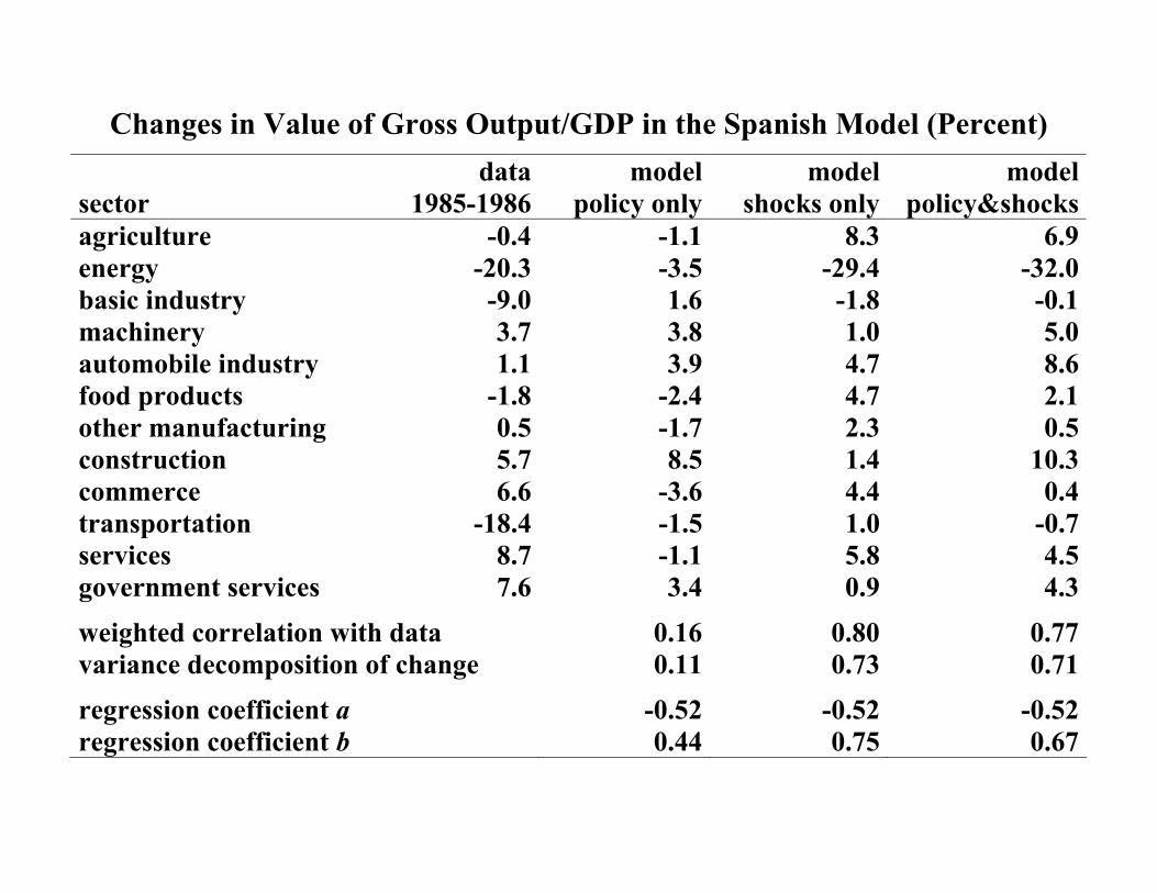
Changes in Value of Gross Output/GDP in the Spanish Model (Percent)

data model model model sector 1985-1986 policy only shocks only policy&shocks agriculture -0.4 -1.1 8.3 6.9 energy -20.3 -3.5 -29.4 -32.0 basic industry -9.0 1.6 -1.8 -0.1 machinery 3.7 3.8 1.0 5.0 automobile industry 1.1 3.9 4.7 8.6 food products -1.8 -2.4 4.7 2.1 other manufacturing 0.5 -1.7 2.3 0.5 construction 5.7 8.5 1.4 10.3 commerce 6.6 -3.6 4.4 0.4 transportation -18.4 -1.5 1.0 -0.7 services 8.7 -1.1 5.8 4.5 government services 7.6 3.4 0.9 4.3

weighted correlation with data 0.16 0.80 0.77 variance decomposition of change 0.11 0.73 0.71

regression coefficient a -0.52 -0.52 -0.52 regression coefficient b 0.44 0.75 0.67

Changes in Trade/GDP

in the Spanish Model (Percent)

data model model modeldirection of exports 1985-1986 policy only shocks only policy&shocksSpain to rest of E.C. -6.7 -3.2 -4.9 -7.8Spain to rest of world -33.2 -3.6 -6.1 -9.3rest of E.C. to Spain 14.7 4.4 -3.9 0.6rest of world to Spain -34.1 -1.8 -16.8 -17.7 weighted correlation with data 0.69 0.77 0.90variance decomposition of change 0.02 0.17 0.24 regression coefficient a -12.46 2.06 5.68regression coefficient b 5.33 2.21 2.37

Changes in Composition of GDP in the Spanish Model (Percent of GDP)

data model model modelvariable 1985-1986 policy only shocks only policy&shockswages and salaries -0.53 -0.87 -0.02 -0.91business income -1.27 -1.63 0.45 -1.24net indirect taxes and tariffs 1.80 2.50 -0.42 2.15

correlation with data 0.998 -0.94 0.99variance decomposition of change 0.93 0.04 0.96

regression coefficient a 0.00 0.00 0.00regression coefficient b 0.73 -3.45 0.85private consumption -0.81 -1.23 -0.51 -1.78private investment 1.09 1.81 -0.58 1.32government consumption -0.02 -0.06 -0.38 -0.44government investment -0.06 -0.06 -0.07 -0.13exports -3.40 -0.42 -0.69 -1.07-imports 3.20 -0.03 2.23 2.10

correlation with data 0.40 0.77 0.83variance decomposition of change 0.20 0.35 0.58

regression coefficient a 0.00 0.00 0.00regression coefficient b 0.87 1.49 1.24

Public Finances in the Spanish Model (Percent of GDP)

data model model model variable 1985-1986 policy only shocks only policy&shocks indirect taxes and subsidies 2.38 3.32 -0.38 2.98 tariffs -0.58 -0.82 -0.04 -0.83 social security payments 0.04 -0.19 -0.03 -0.22 direct taxes and transfers -0.84 -0.66 0.93 0.26 government capital income -0.13 -0.06 0.02 -0.04 correlation with data 0.99 -0.70 0.92 variance decomposition of change 0.93 0.08 0.86 regression coefficient a -0.06 0.35 -0.17 regression coefficient b 0.74 -1.82 0.80

Models of NAFTA Did Not Do a Good Job!

Ex-post evaluations of the performance of applied GE models are

essential if policy makers are to have confidence in the results

produced by this sort of model.

Just as importantly, they help make applied GE analysis a

scientific discipline in which there are well-defined puzzles and

clear successes and failures for alternative hypotheses.

Changes in Trade/GDP in Brown-Deardorff-Stern Model (Percent)

data modelvariable 1988-1999Canadian exports 52.9 4.3Canadian imports 57.7 4.2Mexican exports 240.6 50.8Mexican imports 50.5 34.0U.S. exports 19.1 2.9U.S. imports 29.9 2.3 weighted correlation with data 0.64variance decomposition of change 0.08 regression coefficient a 23.20regression coefficient b 2.43

Changes in Canadian Exports/ GDP in the Brown-Deardorff-Stern Model (Percent)

exports to Mexico exports to United States sector 1988–1999 model 1988–1999 model agriculture 122.5 3.1 106.1 3.4mining and quarrying -34.0 -0.3 75.8 0.4food 89.3 2.2 91.7 8.9textiles 268.2 -0.9 97.8 15.3clothing 1544.3 1.3 237.1 45.3leather products 443.0 1.4 -14.4 11.3footwear 517.0 3.7 32.8 28.3wood products 232.6 4.7 36.5 0.1furniture and fixtures 3801.7 2.7 282.6 12.5paper products 240.7 -4.3 113.7 -1.8printing and publishing 6187.4 -2.0 37.2 -1.6chemicals 37.1 -7.8 109.4 -3.1petroleum and products 678.1 -8.5 -42.5 0.5rubber products 647.4 -1.0 113.4 9.5nonmetal mineral products 333.5 -1.8 20.5 1.2glass products 264.4 -2.2 74.5 30.4iron and steel 195.2 -15.0 92.1 12.9nonferrous metals 38.4 -64.7 34.7 18.5metal products 767.0 -10.0 102.2 15.2nonelectrical machinery 376.8 -8.9 28.9 3.3electrical machinery 633.9 -26.2 88.6 14.5transportation equipment 305.8 -4.4 30.7 10.7miscellaneous manufactures 1404.5 -12.1 100.0 -2.1

weighted correlation with data -0.91 -0.43variance decomposition of change 0.003 0.02

regression coefficient a 249.24 79.20regression coefficient b -15.48 -2.80

Changes in Mexican Exports/GDP in the Brown-Deardorff-Stern Model (Percent)

exports to Canada exports to United States sector 1988–1999 model 1988–1999 model agriculture -20.5 -4.1 -15.0 2.5mining and quarrying -35.5 27.3 -22.9 26.9food 70.4 10.8 9.4 7.5textiles 939.7 21.6 832.3 11.8clothing 1847.0 19.2 829.6 18.6leather products 1470.3 36.2 618.3 11.7footwear 153.0 38.6 111.1 4.6wood products 4387.6 15.0 145.6 -2.7furniture and fixtures 4933.2 36.2 181.2 7.6paper products 23.9 32.9 70.3 13.9printing and publishing 476.3 15.0 122.1 3.9chemicals 204.6 36.0 70.4 17.0petroleum and products -10.6 32.9 66.4 34.1rubber products 2366.2 -6.7 783.8 -5.3nonmetal mineral products 1396.1 5.7 222.3 3.7glass products 676.8 13.3 469.8 32.3iron and steel 32.5 19.4 40.9 30.8nonferrous metals -35.4 138.1 111.2 156.5metal products 610.4 41.9 477.2 26.8nonelectrical machinery 570.6 17.3 123.6 18.5electrical machinery 1349.2 137.3 744.9 178.0transportation equipment 2303.4 3.3 349.0 6.2miscellaneous manufactures 379.4 61.1 181.5 43.2

weighted correlation with data 0.19 0.71variance decomposition of change 0.01 0.04

regression coefficient a 120.32 38.13regression coefficient b 2.07 3.87

Changes in U.S. Exports/GDP in the Brown-Deardorff-Stern Model (Percent)

exports to Canada exports to Mexico sector 1988–1999 model 1988–1999 model agriculture -24.1 5.1 6.5 7.9mining and quarrying -23.6 1.0 -19.8 0.5food 62.4 12.7 37.7 13.0textiles 177.2 44.0 850.5 18.6clothing 145.5 56.7 543.0 50.3leather products 29.9 7.9 87.7 15.5footwear 48.8 45.7 33.1 35.4wood products 76.4 6.7 25.7 7.0furniture and fixtures 83.8 35.6 224.1 18.6paper products -20.5 18.9 -41.9 -3.9printing and publishing 50.8 3.9 507.9 -1.1chemicals 49.8 21.8 61.5 -8.4petroleum and products -6.9 0.8 -41.1 -7.4rubber products 95.6 19.1 165.6 12.8nonmetal mineral products 56.5 11.9 55.9 0.8glass products 50.5 4.4 112.9 42.3iron and steel 0.6 11.6 144.5 -2.8nonferrous metals -20.7 -6.7 -28.7 -55.1metal products 66.7 18.2 301.4 5.4nonelectrical machinery 36.2 9.9 350.8 -2.9electrical machinery 154.4 14.9 167.8 -10.9transportation equipment 36.5 -4.6 290.3 9.9miscellaneous manufactures 117.3 11.5 362.3 -9.4

weighted correlation with data -0.01 0.50variance decomposition of change 0.14 0.02

regression coefficient a 37.27 190.89regression coefficient b -0.02 3.42

Changes in Canadian Trade/GDP in Cox-Harris Model (Percent)

data modelvariable 1988-2000total trade 57.2 10.0trade with Mexico 280.0 52.2trade with United States 76.2 20.0 weighted correlation with data 0.99variance decomposition of change 0.52 regression coefficient a 38.40regression coefficient b 1.93

Changes in Canadian Trade/GDP in the Cox-Harris Model (Percent)

total exports total imports sector 1988-2000 model 1988-2000 model agriculture -13.7 -4.1 4.6 7.2forestry 215.5 -11.5 -21.5 7.1fishing 81.5 -5.4 107.3 9.5mining 21.7 -7.0 32.1 4.0food, beverages, and tobacco 50.9 18.6 60.0 3.8rubber and plastics 194.4 24.5 87.7 13.8textiles and leather 201.1 108.8 24.6 18.2wood and paper 31.9 7.3 97.3 7.2steel and metal products 30.2 19.5 52.2 10.0transportation equipment 66.3 3.5 29.7 3.0machinery and appliances 112.9 57.1 65.0 13.3nonmetallic minerals 102.7 31.8 3.6 7.3refineries 20.3 -2.7 5.1 1.5chemicals and misc. manufactures 53.3 28.1 92.5 10.4

weighted correlation with data 0.49 0.85variance decomposition of change 0.32 0.08 regression coefficient a 41.85 22.00regression coefficient b 0.81 3.55

Changes in Mexican Trade/GDP in the Sobarzo Model (Percent)

exports to North America imports from North America sector 1988–2000 model 1988–2000 model agriculture -15.3 -11.1 -28.2 3.4mining -23.2 -17.0 -50.7 13.2petroleum -37.6 -19.5 65.9 -6.8food 5.2 -6.9 11.8 -5.0beverages 42.0 5.2 216.0 -1.8tobacco -42.3 2.8 3957.1 -11.6textiles 534.1 1.9 833.2 -1.2wearing apparel 2097.3 30.0 832.9 4.5leather 264.3 12.4 621.0 -0.4wood 415.1 -8.5 168.9 11.7paper 12.8 -7.9 68.1 -4.7chemicals 41.9 -4.4 71.8 -2.7rubber 479.0 12.8 792.0 -0.1nonmetallic mineral products 37.5 -6.2 226.5 10.9iron and steel 35.9 -4.9 40.3 17.7nonferrous metals -40.3 -9.8 101.2 9.8metal products 469.5 -4.4 478.7 9.5nonelectrical machinery 521.7 -7.4 129.0 20.7electrical machinery 3189.1 1.0 749.1 9.6transportation equipment 224.5 -5.0 368.0 11.2other manufactures 975.1 -4.5 183.6 4.2

weighted correlation with data 0.61 0.23variance decomposition of change 0.0004 0.002

regression coefficient a 495.08 174.52regression coefficient b 30.77 5.35

What Do We Learn from these Evaluations? The Spanish model seems to have been far more successful in predicting the consequences of policy changes than the three models of NAFTA, but

• Kehoe, Polo, and Sancho (KPS) knew the structure of their

model well enough to precisely identify the relationships between the variables in their model with those in the data;

• KPS were able to use the model to carry out numerical exercises

to incorporate the impact of exogenous shocks. • KPS had an incentive to show their model in the best possible

light.

Sectoral Detail: What Drives Increases In Trade?

Kehoe and Ruhl (2002) Data: four-digit SITC bilateral trade data (789 categories — source: OECD). Exercise:

• rank categories in order of base year exports.

• form sets of categories by cumulating exports the first 2 categories account for 10 percent of exports, for example; the next 4 categories account for 10 percent of exports; and so on.

• calculate the fraction of exports in subsequent years accounted for by each set of categories.

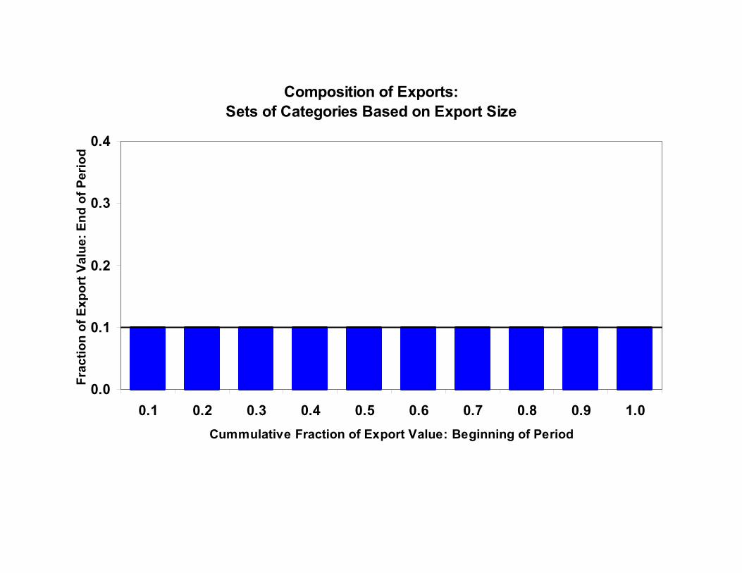
Composition of Exports: Sets of Categories Based on Export Size

0.0

0.1

0.2

0.3

0.4

0.1 0.2 0.3 0.4 0.5 0.6 0.7 0.8 0.9 1.0Cummulative Fraction of Export Value: Beginning of Period

Frac

tion

of E

xpor

t Val

ue: E

nd o

f Per

iod

Composition of Exports: Sets of Categories Based on Export Size

0.0

0.1

0.2

0.3

0.4

0.1 0.2 0.3 0.4 0.5 0.6 0.7 0.8 0.9 1.0Cummulative Fraction of Export Value: Beginning of Period

Frac

tion

of E

xpor

t Val

ue: E

nd o

f Per

iod

Composition of Exports: Canada to Mexico

0.9

1

1.11.31.5

2.45.29.9

24.4

741.3

0.0

0.1

0.2

0.3

0.4

0.1 0.2 0.3 0.4 0.5 0.6 0.7 0.8 0.9 1.0Cummulative Fraction of 1988 Export Value

Frac

tion

of 1

999

Expo

rt V

alue

number of categories in set

Composition of Exports: Mexico to Canada

737.8

24.7

11.8

6 3.3 2

1.30.8

0.7 0.6

0.0

0.1

0.2

0.3

0.4

0.1 0.2 0.3 0.4 0.5 0.6 0.7 0.8 0.9 1.0Cummulative Fraction of 1988 Export Value

Frac

tion

of 1

999

Expo

rt V

alue

number of categories in set

Finished Cars go from 0.8% of exports to 15.0% of exports.

Exports: Canada to Mexico

0.0

0.1

0.2

0.3

0.4

1988 1989 1990 1991 1992 1993 1994 1995 1996 1997 1998 1999

Year

Frac

tion

of T

otal

Exp

ort V

alue

least traded goods in 1988

Exports: Mexico to Canada

0.0

0.1

0.2

0.3

0.4

1988 1989 1990 1991 1992 1993 1994 1995 1996 1997 1998 1999

Year

Frac

tion

of T

otal

Exp

ort V

alue

least traded goods in 1988

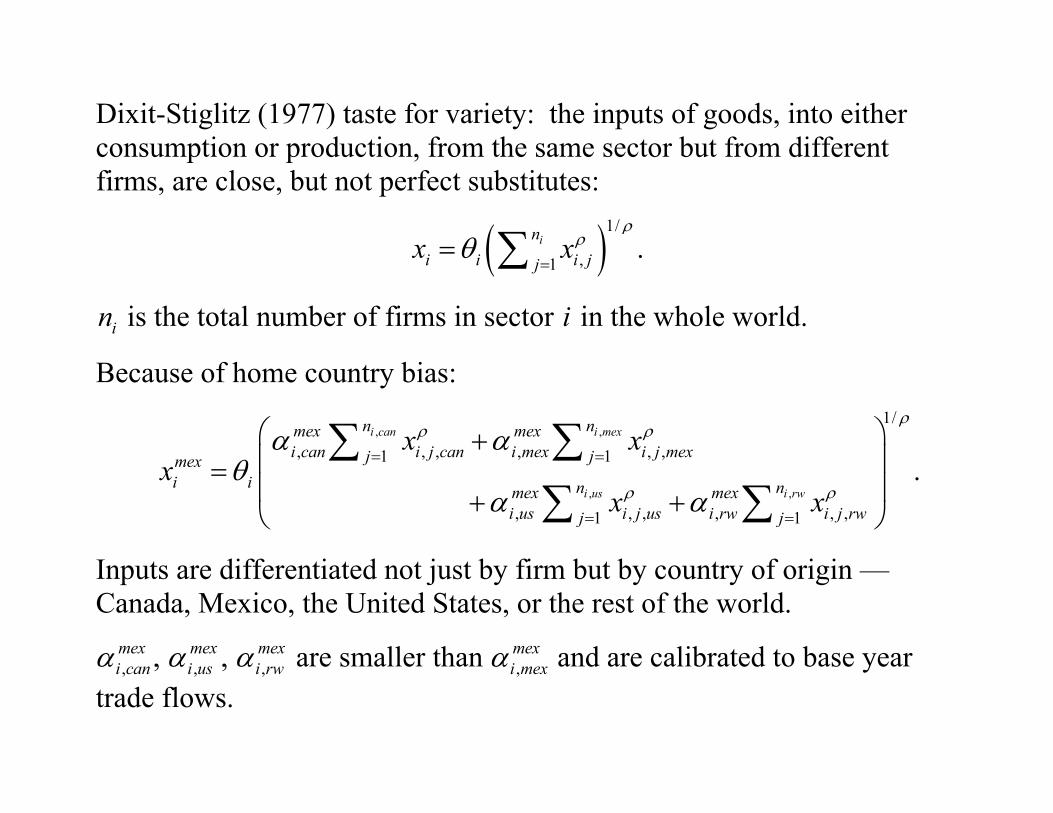
Dixit-Stiglitz (1977) taste for variety: the inputs of goods, into either consumption or production, from the same sector but from different firms, are close, but not perfect substitutes:

( )1/

,1in

i i i jjx x

ρρθ

== ∑ .

in is the total number of firms in sector i in the whole world.

Because of home country bias:

, ,

, ,

1/

, , , , , ,1 1

, , , , , ,1 1

i can i mex

i us i rw

n nmex mexi can i j can i mex i j mexj jmex

i i n nmex mexi us i j us i rw i j rwj j

x xx

x x

ρρ ρ

ρ ρ

α αθ

α α

= =

= =

+ = + +

∑ ∑∑ ∑

.

Inputs are differentiated not just by firm but by country of origin — Canada, Mexico, the United States, or the rest of the world.

,mexi canα , ,

mexi usα , ,

mexi rwα are smaller than ,

mexi mexα and are calibrated to base year

trade flows.

Ricardian model with a continuum of goods [0,1]x∈ production technologies ( ) ( ) / ( )y x x a x= , *( ) *( ) / *( )y x x a x= ad valorem tariffs , *τ τ

(1 *) ( ) * *( )wa x w a xτ+ < ⇔ ( ) **( ) (1 *)

a x wa x wτ

<+

⇒home country produces good and exports it to the foreign country.

( ) (1 ) **( )

a x wa x w

τ+>

⇒foreign country produces good and exports it to the home country.

* ( ) (1 ) *(1 *) *( )

w a x ww a x w

ττ

+< <

+

⇒good is not traded.

Lowering tariffs can generate trade in previously nontraded goods.

( )*( )

a xa x

(1 ) *wwτ+

*(1 *)

wwτ+

x

( )*( )

a xa x

*(1 *)

wwτ+

(1 ) *wwτ+

x

Great Depressions of the Twentieth Century Project

Use growth accounting and applied dynamic equilibrium models to reexamine great depression episodes: United Kingdom (1920s and 1930s) — Cole and Ohanian Canada (1930s) — Amaral and MacGee France (1930s) — Beaudry and Portier Germany (1930s) — Fisher and Hornstein Italy (1930s) — Perri and Quadrini Argentina (1970s and 1980s) — Kydland and Zarazaga Chile and Mexico (1980s) — Bergoeing, Kehoe, Kehoe, and Soto Japan (1990s) — Hayashi and Prescott

(Review of Economic Dynamics, January 2002 revised and expanded version

forthcoming as Minneapolis Fed volume)

Lessons from Great Depressions Project • The main determinants of depressions are not drops in the inputs of

capital and labor — stressed in traditional theories of depressions — but rather drops in the efficiency with which these inputs are used, measured as total factor productivity (TFP).

• Exogenous shocks like the deteriorations in the terms of trade and the

increases in foreign interest rates that buffeted Chile and Mexico in the early 1980s can cause a decline in economic activity of the usual business cycle magnitude.

• Misguided government policy can turn such a decline into a severe and

prolonged drop in economic activity below trend — a great depression.

Big Question: What Drives Changes in Productivity? one-sector growth model maximize [ ]1988

log (1 ) log( )tt t tt

C hN Lβ γ γ∞

=+ − −∑

subject to 1 (1 )( )t t t t t t t t t tC K K w L r K T Xτ δ++ − = + − − + − feasibility constraint

11 (1 ) t t t t t t tC K K X A K Lα αδ −++ − − + = .

tA and tX are treated as exogenous.

Growth Accounting

tY : real GDP (national income accounts)

tX : real investment (national income accounts)

tL : hours worked (labor surveys)

Construct Capital Stocks:

( )1 1t t tK K Xδ+ = − + Total factor productivity is the residual:

1t t t tA Y K Lα α−=

Real GDP per Working-Age Person and Total Factor Productivity in Mexico

90

95

100

105

110

115

1988 1990 1992 1994 1996 1998 2000 2002

year

inde

x (1

988=

100)

Y/N

TFP

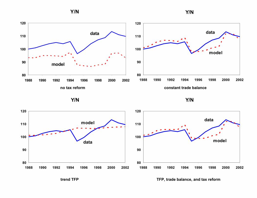
no tax reform constant trade balance

trend TFP TFP, trade balance, and tax reform

Y/N

80

90

100

110

120

1988 1990 1992 1994 1996 1998 2000 2002

data

model

Y/N

80

90

100

110

120

1988 1990 1992 1994 1996 1998 2000 2002

data

model

Y/N

80

90

100

110

120

1988 1990 1992 1994 1996 1998 2000 2002

data

model

Y/N

80

90

100

110

120

1988 1990 1992 1994 1996 1998 2000 2002

data

model

no tax reform constant trade balance

trend TFP TFP, trade balance, and tax reform

L/N

24

26

28

30

32

1988 1990 1992 1994 1996 1998 2000 2002

model

data

L/N

24

26

28

30

32

1988 1990 1992 1994 1996 1998 2000 2002

model

data

L/N

24

26

28

30

32

1988 1990 1992 1994 1996 1998 2000 2002

model

data

L/N

24

26

28

30

32

1988 1990 1992 1994 1996 1998 2000 2002

model

data

no tax reform constant trade balance

trend TFP TFP, trade balance, and tax reform

I/Y

0.00

0.10

0.20

0.30

0.40

1988 1990 1992 1994 1996 1998 2000 2002

data

model

I/Y

0.00

0.10

0.20

0.30

0.40

1988 1990 1992 1994 1996 1998 2000 2002

data

model

I/Y

0.00

0.10

0.20

0.30

0.40

1988 1990 1992 1994 1996 1998 2000 2002

data

model

I/Y

0.00

0.10

0.20

0.30

0.40

1988 1990 1992 1994 1996 1998 2000 2002

data

model

Conjecture: No plausible parameter changes can get the models of NAFTA built on the Dixit-Stiglitz specification to match what has happened in North America. Imposing large elasticities of substitution between different types of goods is capable of generating large increases in trade flows in response to tariff changes, but • it is likely to do so in the wrong sectors; • high elasticities of substitution imply that trade liberalization has very

small welfare consequences; • high elasticities imply implausibly large volatilities of the trade

balance.

If a modeling approach is not capable of reproducing what has

happened, then we should discard it.

Conjecture: The biggest effect of liberalization of trade and capital

flows is on productivity — through changing the distribution of

firms and encouraging technology adoption — rather than the

effects emphasized by the models used to analyze the impact of

NAFTA.