An Evaluation of Model Output Statistics for Subseasonal Streamflow Forecasting inEuropean Catchments

SIMON SCHICK, OLE RÖSSLER, AND ROLF WEINGARTNER

Institute of Geography, and Oeschger Centre for Climate Change Research, University of Bern, Bern, Switzerland

(Manuscript received 10 September 2018, in final form 10 May 2019)

ABSTRACT

Subseasonal and seasonal forecasts of the atmosphere, oceans, sea ice, or land surfaces often rely on Earth

system model (ESM) simulations. While the most recent generation of ESMs simulates runoff per land

surface grid cell operationally, it does not typically simulate river streamflow directly. Here, we apply the

model output statistics (MOS) method to the hindcast archive of the European Centre for Medium-Range

Weather Forecasts (ECMWF). Linear models are tested that regress observed river streamflow on surface

runoff, subsurface runoff, total runoff, precipitation, and surface air temperature simulated by ECMWF’s

forecast systems S4 and SEAS5. In addition, the pool of candidate predictors contains observed precipitation

and surface air temperature preceding the date of prediction. The experiment is conducted for 16 European

catchments in the period 1981–2006 and focuses onmonthly average streamflow at lead times of 0 and 20 days.

The results show that skill against the streamflow climatology is frequently absent and varies considerably

between predictor combinations, catchments, and seasons. Using streamflow persistence as a benchmark

model further deteriorates skill. This is most pronounced for a catchment that features lakes, which extend to

about 14% of the catchment area. On average, however, the predictor combinations using the ESM runoff

simulations tend to perform best.

1. Introduction

Subseasonal and seasonal forecasts of environmental

conditions are increasingly based on numerically cou-

pled models of the various Earth system components.

These include general circulation models of the atmo-

sphere and oceans and dynamical land surface or sea ice

models (National Academies 2016).

Such forecast systems represent diverse physical, chem-

ical, and biological processes and continuously progress to-

ward Earth system models (ESMs). However, not all

environmental variables of interest are resolved. For exam-

ple, current generation ESMs simulate runoff per land sur-

face grid cell operationally, but they donot typically simulate

river streamflow (Clark et al. 2015; Yuan et al. 2015).

To the best of our knowledge, ESM runoff simulations

have been virtually ignored for subseasonal and sea-

sonal streamflow forecasting with the exception of the

following studies:

d Yuan andWood (2012) predict seasonal streamflow in the

Ohio basin using hindcasts of theClimate Forecast System

version 2 (CFSv2). Besides forcing the VIC hydrological

model with CFSv2 climate predictions, the authors also

postprocess the CFSv2 runoff simulations with a linear

routing model and a statistical bias correction. The results

highlight the importance of the statistical bias correction

and show that the postprocessed runoff simulations pro-

vide a serious benchmark for the calibrated VIC model.d Emerton et al. (2018) introduce theGlobal FloodAware-

ness System (GloFAS) seasonal forecasting system. This

system builds upon the forecasting capabilities of the

European Centre for Medium-RangeWeather Forecasts

(ECMWF) and feeds runoff simulated by the ESM land

surface scheme to the LISFLOOD model: Subsurface

runoff enters a groundwater module and streamflow is

routed according to the kinematic wave equations.

A different approach to predict river streamflow with

ESM-based runoff simulations exists in the application of

the model output statistics (MOS) method. The MOS

method emerged in the context of weather prediction

(Glahn and Lowry 1972; Klein and Glahn 1974), where it

regressed the variable of interest against the output of a

numerical weather model. Today, the MOS method usu-

ally has to deal with an ensemble of model integrations,Corresponding author: Simon Schick, simon.schick@giub.unibe.ch

JULY 2019 S CH I CK ET AL . 1399

DOI: 10.1175/JHM-D-18-0195.1

� 2019 American Meteorological Society. For information regarding reuse of this content and general copyright information, consult the AMS CopyrightPolicy (www.ametsoc.org/PUBSReuseLicenses).

Unauthenticated | Downloaded 02/13/22 01:08 PM UTC

which accounts for uncertainties regarding the initial condi-

tions and model implementation (e.g., Schefzik et al. 2013).

Broadly speaking, the MOS method attempts to sta-

tistically model the correlation of dynamical forecasts

and corresponding observations. Besides the prediction

of variables not resolved by the dynamical model, the

MOS method also can target bias correction (Barnston

and Tippett 2017), model combination (Slater et al.

2017), and the modeling of the forecast’s probability

distribution (Zhao et al. 2017). Often, several of these

targets are addressed at the same time.

The MOS method is also sporadically used to predict

river streamflowat the subseasonal and seasonal time scales.

Early examples include Landman and Goddard (2002) and

Foster andUvo (2010), while more recently the approaches

of Sahu et al. (2017), Lehner et al. (2017), or Slater and

Villarini (2018) fall within the realm of the MOS method.

Inmost of these studies, the predictand consists of (sub)

seasonal streamflow volumes and the model formulation

is based on the assumption of linear predictor–predictand

relationships. However, the selected predictors vary

considerably and include ESM-simulated precipitation,

wind velocity, surface air temperature, the geopotential

height of atmospheric pressure levels, or time series of

land use cover and population density.

Here, we test the application of the MOS method to

ESM-based subseasonal forecasts of surface, subsurface,

and total runoff. In addition, models are formulated that

include precipitation and surface air temperature as pre-

dictors. The present implementation of the MOS method

relies on the linear regression model and is prototyped in

Schick et al. (2018). Tomature the prototypewe add an error

model and conduct a validation in 16European river systems

featuring a range of climatic and geographical conditions.

The hindcast experiment uses data from both the

former (S4) as well as current (SEAS5, or S5 in short)

seasonal forecast systems of ECMWF. To separate the

skill originating from the traditional weather forecasting

time scale and the potential skill at the subseasonal time

scale, the predictand is defined as mean streamflow of a

time window of 30 days with lead times of 0 and 20 days.

Below, section 2 introduces the dataset, section 3 de-

tails the MOS method and the hindcast verification,

sections 4 and 5 present and discuss the results, and

section 6 concludes the study.

2. Data

Thehydrometeorological data cover the timeperiod1981–

2006 and have a daily temporal resolution. Spatial fields get

aggregated by taking catchment area averages based on the

percent of grid cell coverage of the catchment polygon. In

addition, each grid cell is weighted by the cosine of its

latitude to account for the meridional variation of the grid

cell area.

a. Catchments

Table 1 and Fig. 1 show the set of the selected 16

catchments, which includes lowlands and mountainous

regions as well as subarctic, temperate, mediterranean,

and humid-continental climate types (Peel et al. 2007;

Mücher et al. 2010). The catchment areas approximately

range from 5000 to 285 600km2.

These river systems are subject to damming and

streamflow regulation of varying degree (Nilsson et al.

2005). However, human activities affecting river stream-

flow can hardly be avoided when it comes to streamflow

forecasting in large European river systems. Whether

these human activities lead to a pattern that can be

learned by the MOS method or instead are a source of

noise will be discussed later in more detail.

b. Observations

Daily mean streamflow observations (m3 s21) are

provided by the Global Runoff Data Centre (GRDC

2016), the SpanishMinistry ofAgriculture and Fisheries,

Food and Environment (MAFFE 2017), and the French

Ministry for an Ecological and Solidary Transition

(MEST 2017). Catchment polygons are either retrieved

from the GRDC (2016) or derived from the European

catchments and Rivers network system (ECRINS 2012).

Daily observations of surface air temperature (8C) andprecipitation (mm) are taken from the ENSEMBLES

gridded observational dataset in Europe, version 16.0 (E-

OBS). This dataset is based on a statistical interpolation

of weather station observations and is available on a 0.258regular grid (Haylock et al. 2008; E-OBS 2017).

c. Hindcast archive

ECMWF’s former (S4) and current (S5) seasonal fore-

cast systems consist of numerically coupled atmosphere–

ocean–land models; in addition, S5 includes the LIM2 sea

icemodel. The net horizontal resolution of the atmosphere

model equals about 80km (S4) and 35km (S5), whereas

the NEMO ocean model approximately operates on a 18(S4) and 0.258 (S5) grid (ECMWF 2017).

The HTESSEL land surface model, which is part of

both S4 and S5, dynamically divides each grid cell into

fractions of bare ground, low and high vegetation, inter-

cepted water, snow, and snow under high vegetation. The

partitioning into infiltration and surface runoff happens

according to the Arno scheme. Vertical water flow in the

soil, which is discretized into four layers with a total depth

of about 3m, follows the Richards equation. Total runoff

finally equals the sumof surface runoff and open drainage

at the soil bottom (Balsamo et al. 2009; ECMWF 2018).

1400 JOURNAL OF HYDROMETEOROLOGY VOLUME 20

Unauthenticated | Downloaded 02/13/22 01:08 PM UTC

For both S4 and S5 the hindcast spans back to 1981 with

initial conditions taken from ERA-Interim. Reforecasts

are initialized on the first day of each month and simulate

the subsequent 7 months. The number of hindcast en-

semble members equals 15 (S4) and 25 (S5), respectively.

Please note that this describes ECMWF’s standard hind-

cast configuration, that is, for certain dates of prediction

more ensemble members and a longer lead time are

available.

We downloaded the following variables on a regular

0.758 (S4) and 0.48 (S5) grid at a daily resolution: accu-

mulated precipitation (m), air temperature 2m above

ground (K), accumulated total runoff, surface runoff,

and subsurface runoff (m). Surface and subsurface

runoff is only available for the S5 system.

After taking catchment area averages as described

above, accumulated variables are first converted to daily

fluxes; in addition, total runoff, surface runoff, and sub-

surface runoff are converted from meters (m) to meters

cubed per second (m3 s21) and surface air temperature is

converted from kelvins (K) to degrees Celsius (8C). Fi-nally, the ensemble gets compressed to its mean value.

3. Method

The predictand yw,l denotes mean streamflow (m3 s21)

of a time window with length w5 30 days and lead time

l5 0, 20 days. Here, lead time is defined as the time dif-

ference between the date of prediction and the onset of

the actual prediction window w. The date of prediction is

set to the first day of the month in the period 1981–2006.

To predict with a 20-day lead time, we do not regress

y30,20, but instead predict y20,0 and y50,0, followed by in-

tegration in time and taking differences, that is,

y30,20

5 (y50,0

3 502 y20,0

3 20)/30 . (1)

Doing so allows us to center the model formulation

around the date of prediction without the need to ac-

count for the temporal gap introduced by the lead time l

(section 3a).

Thus, for the regressionwe effectively usew5 30, 30, 50

days and l5 0 days. Furthermore, the modeling procedure

is individually applied for each prediction window w and

TABLE 1. Selected catchments and corresponding sites of gauging stations, data providers, catchment areas, and average streamflows in

the period 1981–2006.

Name Site Provider Catchment area (km2) Average streamflow (m3 s21)

1 Angerman Sollefteå GRDC 30 900 532

2 Danube Bratislava GRDC 131 400 2072

3 Duero Herrera de Duero MAFFE 12 900 24

4 Elbe Neu-Darchau GRDC 131 100 691

5 Garonne Lamagistère MEST 32 300 386

6 Glama Langnes GRDC 39 900 702

7 Kemijoki Isohaara GRDC 53 900 577

8 Lower Bann Movanagher GRDC 5000 92

9 Neva Novosaratovka GRDC 285 600 2479

10 Oder Hohensaaten-Finow GRDC 110 500 492

11 Rhine Lobith GRDC 159 400 2335

12 Rhone Beaucaire MEST 95 800 1707

13 Seine Paris MEST 43 600 315

14 Tisza Senta GRDC 141 100 795

15 Torne Kukkolankoski GRDC 40 500 423

16 Trent Colwick GRDC 7500 84

FIG. 1. The hindcast experiment is conducted for 16 catchments

situated in Europe. Black crosses on a yellow background indicate

the sites of the gauging stations, light blue lines show some large

rivers, and the numbers refer to the entries in Table 1. The map is

produced with data from Natural Earth (2018).

JULY 2019 S CH I CK ET AL . 1401

Unauthenticated | Downloaded 02/13/22 01:08 PM UTC

date of predictionwithin the calendar year, leaving 26 years

to perform the regression. Having said this, we drop for the

following the subscripts w and l.

a. Regression model

1) TIME AGGREGATION SCREENING

The time aggregation of a particular predictor is de-

fined with respect to the date of prediction and involves

summation (precipitation) or averaging (surface air

temperature and runoff) in time. The time aggregation

period is not fixed in advance, but is individually selected

for each predictor based on the linear correlation with y.

It is constrained to the sets

d Apre 5 f10, 20, . . . , 720g days for predictors that carryinformation preceding the date of prediction (back-

ward in time; columns x1 and x2 in Table 2), andd Asub 5 f5, 10, . . . , 200g days for predictors that carry

information subsequent to the date of prediction

(forward in time; columns x3 and x4 in Table 2).

For the refRun model (introduced below) we set

Asub 5 f5, 10, . . . , w1 lg days.

In so doing the time window of the ESM-based pre-

dictors can differ from the actual forecast window. This

allows us to account for a delayed catchment response to

the atmospheric forcings or could help to better detect

skillfully predicted climate anomalies.

2) PREDICTOR COMBINATIONS

The regression equation is given by

y5c(x,D)1 «5 xTb1 « , (2)

with xT 5 [1x1x2x3x4] being the predictor vector and b

the coefficient vector. Both the time aggregation periods

of the entries in x as well as the ordinary least squares

estimate ofb are based on the training setD. Please note

that we do not make any distributional assumption

about the error term «.

Table 2 shows the different predictor combinations

that make up x. The models named refRun (reference

run) and preMet (preceding meteorology) are intended

to provide an upper and lower boundary of prediction

skill when using precipitation and surface air temperature

as predictors: For the refRun model we plug in observed

precipitation and surface air temperature preceding the

date of prediction (i.e., a proxy for the initial hydrological

conditions) as well as observed precipitation and surface

air temperature subsequent to the date of prediction (i.e.,

assuming perfect seasonal climate predictions). In con-

trast, the preMet model does not have any information

about the climate of the target period.

The remaining models contain predictors from the S4

and S5 hindcast archives, which all base on the ensemble

mean: besides precipitation and surface air temperature,

we test total runoff as well as surface and subsurface

runoff as individual predictors. Please see appendix A

for a technical note concerning the S5sro1ssro model.

3) BOOTSTRAP AGGREGATING

Bootstrap aggregating (bagging) dates back toBreiman

(1996a) and is a technique to reducemodel variance. For

the present prediction problem and modeling strategy,

bagging helps to stabilize model variance as introduced

by the small sample size and the sometimes weak re-

lationships (Schick et al. 2016). The bagged prediction

follows

y51

b�b

j51

c(x,Dj), (3)

where the subscript j indicates the jth nonparametric

bootstrap replicate ofD. Please note that the number of

TABLE 2. The predictor combinations consider the variables p: precipitation, t: surface air temperature, ro: total runoff, sro: surface

runoff, and ssro: subsurface runoff. Predictors get aggregated in time either preceding or subsequent to the date of prediction; the

subscripts indicate the data source, i.e., the E-OBS dataset and the S4 and S5 hindcast archives. Predictors derived from the S4 and S5

archives are based on the ensemble mean.

Preceding Subsequent

Name x1 x2 x3 x4 Description

refRun pE-OBS tE-OBS pE-OBS tE-OBS Precipitation and temperature from the E-OBS dataset

preMet pE-OBS tE-OBS — — Precipitation and temperature from the E-OBS dataset

S4PT pE-OBS tE-OBS pS4 tS4 Precipitation and temperature from the E-OBS dataset

and S4 archive

S5PT pE-OBS tE-OBS pS5 tS5 Precipitation and temperature from the E-OBS dataset

and S5 archive

S4ro — — roS4 — Total runoff from the S4 archive

S5ro — — roS5 — Total runoff from the S5 archive

S5sro1ssro — — sroS5 ssroS5 Surface and subsurface runoff from the S5 archive

1402 JOURNAL OF HYDROMETEOROLOGY VOLUME 20

Unauthenticated | Downloaded 02/13/22 01:08 PM UTC

bootstrap replicates b should not be regarded as a

tuning parameter, but is set to a value such that the

prediction error stabilizes. To guarantee the robustness

of the analysis we set b5 100, which can be consid-

ered as rather high [e.g., Breiman (1996a) recommends

b 2 f25, . . . , 50g].b. Error model

The error model employs the so-called ‘‘out-of-bag’’

prediction error estimate (Breiman 1996b), which avoids an

additional cross validation. In each of the b bootstrap rep-

licates we (most likely) miss some of the cases contained in

the full training set. Thus, for the ith case (yi, xi) 2 D we

can approximate its prediction error according to

«i5 y

i2

1

�b

j51

1(yi;D

j)

�b

j51

c(xi,D

j)3 1(y

i;D

j), (4)

with 1(�) denoting the indicator function that returns

one if its argument evaluates to true and zero otherwise.

Here, the indicator function excludes those models from

the model averaging in Eq. (3) that use (yi, xi) for the

time aggregation screening and estimation of b. For the

20-day lead time, Eq. (4) needs to be adapted according

to Eq. (1).

Having estimated the prediction error for each case in the

training set, we then use a kernel density estimate to specify

the probability density function f of a future prediction y

f (y)51

nh�n

i51

K

�y2 y2 «

i

h

�, (5)

with n being the sample size of the training setD and the

kernel K(z) the standard Gaussian density function

K(z)51ffiffiffiffiffiffi2p

p exp

�21

2z2�. (6)

The bandwidth parameter h. 0 is automatically se-

lected according to the method of Sheather and Jones

(1991) as implemented in the statistical software R

(R Core Team 2018). This method belongs to the ‘‘solve-

the-equation plug-in’’ approaches and relies on the mini-

mization of the asymptotic mean integrated squared error

(AMISE). The method seems to work well for a variety of

density shapes as it uses a bandwidth independent of h to

estimate the second derivative of the unknown density

function in the AMISE (Jones et al. 1996).

c. Verification

The modeling procedure outlined in sections 3a and

3b is subject to a buffered leave-one-out scheme. A

buffer of 2 years to the right and left of the left-out year

is used in order to avoid artificial skill due to hydrome-

teorological persistence (Michaelsen 1987).

The persistence benchmark model [section 3c(5) be-

low] requires streamflow observations preceding the date

of prediction. Since we do not have streamflow observa-

tions prior to January 1981, wemiss the predictions of the

persistence model in January 1981. Thus, we decide to

exclude January 1981 for the entire verification.

1) RELIABILITY

Reliable forecast distributions reproduce the observa-

tions’ frequency, that is, the forecast distribution is neither

too narrow (overconfident) nor toowide (underconfident).

Here, we follow Laio and Tamea (2007), who propose to

evaluate the probability integral transform (PIT) values

graphically via the empirical cumulative distribution

function. The PIT value of a forecasted cumulative distri-

bution function F i(y) and corresponding observation yi is

defined as the probability

PIT5 Fi(y

i) . (7)

If y is continuous and the forecasts are reliable, the PIT

values follow the uniform distribution U(0, 1).

2) ASSOCIATION AND ACCURACY

The following scoring rules are employed: the linear

correlation coefficient of the predictions and observa-

tions, the mean absolute error (MAE), the mean squared

error (MSE), and the continuous ranked probability

score (CRPS). The CRPS, averaged over n cases in the

hindcast period, is defined as (Hersbach 2000)

CRPS51

n�n

i51

ð‘2‘

[Fi(y)2H(y2 y

i)]2 dy , (8)

with H(�) denoting the Heaviside function

H(x)5

�0, x, 0,

1, x$ 0:(9)

3) SKILL

Having a model of interest m1 and benchmark model

m2, themean absolute error skill score (MAESS) is then

defined as

MAESS5 12MAEm1

MAEm2. (10)

The mean squared error skill score (MSESS) and the

continuous ranked probability skill score (CRPSS) are

defined analogously.

JULY 2019 S CH I CK ET AL . 1403

Unauthenticated | Downloaded 02/13/22 01:08 PM UTC

4) STATISTICAL SIGNIFICANCE

Statistical tests are conducted conditional on the date

of prediction within the calendar year (thus n5 26):

d To test the PIT values for uniformity, we report the

number of null hypothesis rejections of the Pearson’s

chi-squared test using four, five, and six equally sized

bins. In addition, we use confidence bands based on

the Kolmogorov–Smirnov test. In both cases the null

hypothesis assumes a uniform distribution, so we set

the significance level to 0.25 in order to have more

control on the type II error (that is not rejecting the

null hypothesis when it is in fact false). The value of

theKolmogorov–Smirnov test statistic at the 0.25 level

is taken from D’Agostino and Stephens (1986).d To test whether a model m1 and a benchmark m2

differ in terms of the MSE and CRPS, we use paired

differences of the individual squared errors and CRPS

values. The null hypothesis ‘‘the mean difference

equals zero’’ is then tested with the two-sided t test.

It must be noted that the paired differences do not

always follow a Gaussian distribution. However, a

comparison with a nonparametric bootstrap and the

Wilcoxon test showed that the t test leads to the most

conservative results, for that reason we only report the

p values of the t test.

5) ADDITIONAL MODELS

To help in the interpretation of the forecast quality

and to benchmark the MOS method, the following ad-

ditional models are used:

d climatology—the average of the predictand in the

period 1981–2006;d trend—a linear trend model for the predictand;d persistence—a linear regression of the predictand

against observed mean streamflow of the 30 days

preceding the date of prediction;d S4ro.lm, S5ro.lm, and S5sro1ssro.lm—a linear regres-

sion of the predictand against the runoff simulations of

the same time window (lm stands for linear model).

The S4ro.lm, S5ro.lm, and S5sro1ssro.lm models can

be considered as simpler versions of their counterparts

in Table 2 in that they neither employ Eq. (1) nor the

time aggregation screening and bagging; this resembles

the approach of Balsamo et al. (2015) to verify the ERA-

Interim/Land simulation with respect to river stream-

flow observations.

Identical to the models of Table 2, the above listed

models condition on the date of prediction within the

calendar year, they undergo the cross validation, and the

forecast distribution is based on the kernel density

estimate from Eq. (5). However, the residuals «i are the

in-sample prediction errors of the training set.

4. Results

To get an overview we first calculate the correlation,

MAESS, and MSESS using the complete time series of

observations and predictions. Based on this overview, we

decide at which models to look in more detail. This is

subsequently done by verifying the hindcast conditional

on the date of prediction within the calendar year, vali-

dating the reliability of the error model, and conducting a

probabilistic verification in terms of the CRPS.

Below, we frequently switch between scoring rules

in a seemingly unmotivated fashion. However, this helps

us in section 5f to put the hindcast results into context

with other studies. In addition, the usage of both de-

terministic and probabilistic scoring rules enables to

validate the regression model (section 3a) separately

from the error model (section 3b).

a. Overview

Figure 2 shows per catchment and model the linear

correlation coefficient of the predictions and correspond-

ing observations as well as the MAESS and MSESS with

the climatology as benchmark. In general, we can identify

four groups of models with a distinct performance:

d The correlation of the climatology can go up to about 0.8

with the median being around 0.5, showing that several

streamflow time series exhibit a pronounced periodic

component. The trend model does not show any im-

provement over the climatology, which consequently

manifests in a MAESS and MSESS around zero.d The persistence model shows a marked improvement

over the climatology and the trend model; it performs

often on a level close to the preMet model and the

models using the S4 and S5 simulations. This model

tends to have the largest performance variability, in

particular for the MSESS, where the positive outlier

belongs to the Neva and the negative outlier to the

Duero catchment. On average, the persistence model

reduces the MAE of the climatology by about 18%

(i.e., MAESS of 0.18) and the MSE of the climatology

by about 23% (i.e., MSESS of 0.23) at the 0-day lead

time. At the 20-day lead time, the corresponding

reductions amount to 8% (MAE) and 4% (MSE).d The preMet model and the models that use the S4 and

S5 simulations often end up with a similar perfor-

mance. However, it seems that the runoff-based

models score best. On average, the models in this

group reduce the MAE of the climatology by about

25% and the MSE of the climatology by about 40% at

the 0-day lead time. At the 20-day lead time, the

1404 JOURNAL OF HYDROMETEOROLOGY VOLUME 20

Unauthenticated | Downloaded 02/13/22 01:08 PM UTC

corresponding reductions amount to 9% (MAE) and

15% (MSE).d The refRun model scores on average a correlation of

about 0.85 and decreases the MAE of the climatology by

about 35%and theMSEof the climatologyby about 55%.

For the following, we take a closer look at the S4PT,

S5PT, S4ro, and S5ro models: the S4PT and S5PT models

are retained as they do not use the runoff simulations.

The S4ro and S5ro models are used to represent the

runoff-based models, which all perform on a similar level;

however, for the S5ro model we observe a negative

MSESS outlier at the 20-day lead time, which could be

interesting to investigate. In addition, the climatology,

trend, persistence, preMet, and refRun models are

retained for interpretation and benchmarking.

b. Linear correlation

The correlation coefficient per date of prediction

within the calendar year, pooled to seasons, is shown in

FIG. 2. Linear correlation, MAESS, and MSESS per model and catchment, based on the complete time series of predictions and

observations. Shown are the (top) 0-day lead time and (bottom) 20-day lead time. TheMAESS andMSESS are computed with respect to

the streamflow climatology; n 5 16.

FIG. 3. Linear correlation between predictions and observations for each catchment and date of prediction within the calendar year,

pooled to seasons. The dashed lines indicate the confidence intervals under the null hypothesis of zero correlation at the 0.05 and 0.01

significance level (t test for the correlation coefficient of a bivariate, normally distributed sample). Shown are the (top) 0-day lead time and

(bottom) 20-day lead time; n 5 48.

JULY 2019 S CH I CK ET AL . 1405

Unauthenticated | Downloaded 02/13/22 01:08 PM UTC

Fig. 3. The dashed lines indicate the statistical signifi-

cance at the 0.05 and 0.01 levels under the null hypoth-

esis of zero correlation (t test for the correlation

coefficient of a bivariate, normally distributed sample).

In general, we observe only little seasonal variation

both at the 0-day as well as the 20-day lead time, but

instead a large within-season variability. Aside from the

trend and refRun models, the correlation varies around

0.5 at the 0-day lead time and around 0.25 at the 20-day

lead time, the latter value no longer being statistically

significant. For the trend model, the correlation is

mostly negative, whereas the refRun model scores a

correlation around 0.7.

c. MSESS

Figures 4 and 5 show theMSESS conditional on the date

of prediction within the calendar year with the climatology

as benchmark. If the paired differences in the MSE can be

assumed to differ from zero according to the t test, a large

(small) cross is drawn in the case of the 0.01 (0.05) signifi-

cance level. The top rows correspond to the 0-day lead time

and the bottom rows to the 20-day lead time.

For the models using the S4 and S5 simulations (Fig. 4),

we observe in most cases positive skill at the 0-day lead

time, however, the statistical significance is frequently ab-

sent. Significant positive skill tends to cluster in spring,

though a clear overall pattern does not emerge. Instead skill

varies between catchments, dates of prediction, andmodels.

At the 20-day lead time skill gets drastically reduced.

Exceptions are the Oder, where the S4ro and S5ro

models are not much degraded compared to the 0-day

lead time, and the Neva, for which the S4PT and S5PT

models still score positive skill. Here, it is also visible

that the negative outlier produced by the S5ro model in

Fig. 2 belongs to the Lower Bann.

The Oder and Neva show some further features

(Figs. 4 and 5):

d For the Oder, we observe that the S4ro and S5ro

models perform well. On the other hand, the models

using the meteorological predictors, including the

refRun model, perform poorly.d The Neva seems to be the only catchment in which a

linear trend contributes to skill against climatology in

several months. Furthermore, the persistence, pre-

Met, S4PT, and S5PT models score above average,

while the S4ro and S5ro models instead show almost

no skill.

FIG. 4. MSESS at the (top) 0-day and (bottom) 20-day lead timewith the streamflow climatology as the benchmark. Themonths refer to

the date of prediction. The p values smaller than 0.01 (0.05) for the null hypothesis ‘‘no difference in the MSE value’’ are indicated with a

large (small) cross; n 5 26.

1406 JOURNAL OF HYDROMETEOROLOGY VOLUME 20

Unauthenticated | Downloaded 02/13/22 01:08 PM UTC

d. Reliability

Figure 6 shows the PIT values for those models that

get verified in terms of the CRPS in the next section.

Shown are the empirical cumulative distribution func-

tions of the PIT values at the 0-day lead time for each

date of prediction within the calendar year, but pooled

to seasons.

The distributions are accompanied by the Kol-

mogorov confidence bands at the 0.25 significance

level. The numbers in the top-left corner report

the number of rejected null hypotheses of the chi-

squared test based on four, five, and six bins, again at

the 0.25 level. The histograms at the bottom finally

pool all PIT values across seasons and catchments.

In general, we observe that the PIT distributions of

the S4ro and S5ro models tend to better align with the 1:

1 diagonal than the PIT distributions of the preMet,

S4PT, and S5PT models. Concerning the statistical sig-

nificance, the PIT values are almost never outside the

Kolmogorov confidence band. The chi-squared test re-

jects on average about four out of 48 distributions from

being reliable.

Persistent departures from uniformity are more clear in

the histograms at the bottom of Fig. 6. For all models we

observe a trend toward underconfidence, that is, the

tails of the forecast distributions are too heavy. For the

20-day lead time (not shown), the overall picture re-

mains the same.

e. CRPSS

Figure 7 is similar to Figs. 4 and 5, but employs the

CRPSS with the preMet model as the benchmark. Thus,

for the S4PT and S5PT models skill solely originates

from the S4 and S5-predicted precipitation and surface

air temperature.

Starting with the 0-day lead time (top row), we ob-

serve for the S4PT and S5PT models some positive skill

scattered among the catchments and dates of prediction.

The S4ro and S5ro models in general do a better job,

which is most evident for the Oder. On the other hand,

these models score some large negative CRPSS values.

At the 20-day lead time (bottom row), skill of the

S4PT and S5PT models virtually drops to zero, while

the S4ro and S5ro models are still able to outperform

the preMet model, most notably in the case of the

Oder.

FIG. 5. MSESS at the (top) 0-day and (bottom) 20-day lead time with the streamflow climatology as the benchmark. Themonths refer to

the date of prediction. The p values smaller than 0.01 (0.05) for the null hypothesis ‘‘no difference in the MSE value’’ are indicated with a

large (small) cross; n 5 26.

JULY 2019 S CH I CK ET AL . 1407

Unauthenticated | Downloaded 02/13/22 01:08 PM UTC

f. Persistence model

The results frequently indicate that the persistence

benchmark model is challenging to beat in several

catchments. Thus, appendix B contains Figs. 2, 4, 5,

and 7 using the persistence model as the bench-

mark in the calculation of the MAESS, MSESS, and

CRPSS (see Figs. B1–B4). The main results are as

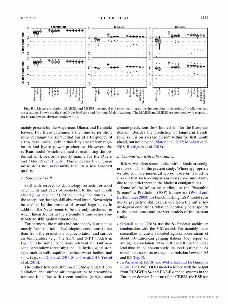
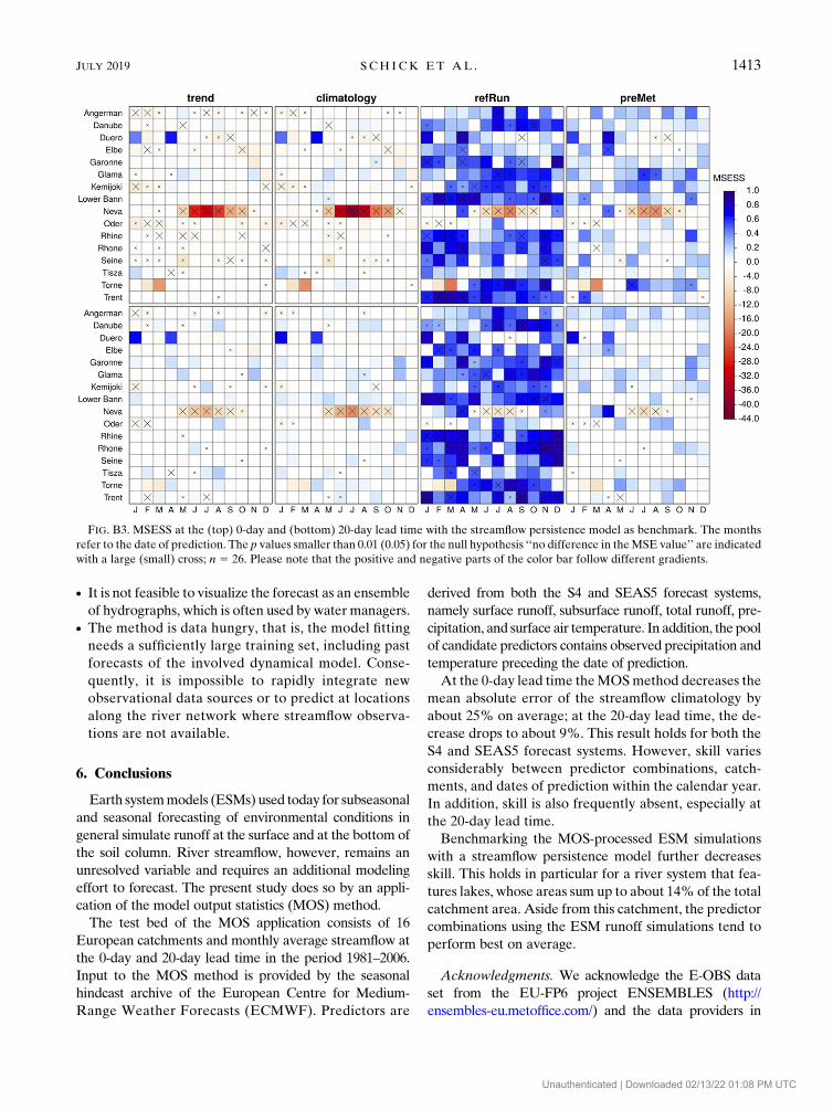
follows:

d One strong negative outlier is present for almost all

models (see Fig. B1). This outlier with MAESS and

MSESS values in the range from20.5 to22 belongs to

the Neva. Otherwise, the MAESS scatters around 0.1

(0-day lead time) and 0.0 (20-day lead time), and the

MSESS scatters around 0.25 (0-day lead time) and 0.1

(20-day lead time).d The Neva catchment stands out as well in the other

figures in appendix B (see Figs. B2, B3, and B4).MSESS

values range down to 244 and CRPSS values range

down to 25.5. Otherwise, positive skill is either ab-

sent (in particular at the 20-day lead time) or does not

follow an easy to interpret pattern.

5. Discussion

First, we discuss the validity of the regression and error

models from a technical point of view. Second, we contrast

the different predictor combinations. Third, we discuss the

role of anthropogenic signals in the streamflow time series

and potential sources of forecast skill. Finally, we compare

the present hindcast results with results reported in other

studies and gather the pros and cons of the MOS method.

a. Regression model

1) TIME AGGREGATION

The MOS method aims at modeling the correlation

between dynamical forecasts and observations of the

FIG. 6. Empirical cumulative distribution of the PIT values obtained at the 0-day lead time. The

distribution is individually plotted for each catchment and date of prediction within the calendar

year (n5 26) but pooled to seasons. The number of null hypothesis rejections of the chi-squared test

are reported in the top left corner (corresponding to four, five, and six bins at the 0.25 significance

level); the dashed red lines indicate the Kolmogorov 0.25 confidence band. The histograms at the

bottom pool all PIT values across seasons and catchments [n5 (263 122 1)3 165 4976].

1408 JOURNAL OF HYDROMETEOROLOGY VOLUME 20

Unauthenticated | Downloaded 02/13/22 01:08 PM UTC

target variable. Apart from long-term trends and sea-

sonal patterns, this correlation emerges at the (sub)

seasonal time scale only at a low temporal resolution, if

present at all (Troccoli 2010). The MOS method thus

depends on a suitable time averaging applied to the in-

volved variables and inevitably operates at a low tem-

poral resolution.

The S4ro.lm, S5ro.lm, and S5sro1ssro.lm benchmark

models do not apply a time aggregation screening, but

instead regress the predictand against the runoff simu-

lations of the same 30-day time window. The results

show that these benchmarks compete well against their

counterparts (i.e., S4ro, S5ro, and S5sro1ssro; Fig. 2).

Thus, for the predictors that carry the runoff simulations

the additional effort of the time aggregation screening

only leads to small improvements.

2) LINEARITY

The model formulation strictly assumes a linear re-

lationship between the predictors and the predictand.

From both an empirical as well as theoretical point of

view, the assumption of linearity gains validity with an

increasing time aggregation window length (Yuval and

Hsieh 2002; Hsieh et al. 2003).

The residual analysis (not shown) reveals that low flows

tend to be overpredicted and high flows tend to be

underpredicted, often leading to skewed residual distribu-

tions. In addition, the pooled time series of the residuals

sometimes exhibit autocorrelation. These issues could be

related to missing predictors or imply that the time aver-

aging windows of 20, 30, and 50 days are too short to

completely linearize the predictor–predictand relationship.

However, the assumption of linearity is a technical

constraint, too: Extrapolation beyond the domain covered

by the training set leads to a few poor predictions, espe-

cially as some outliers are present in the S4 and S5 runoff

simulations. For example, one of these outliers causes the

large negative MSESS of the S5ro model in Fig. 4 for

the Lower Bann. Subsequently, poor predictions become

disastrous predictions when introducing interactions or

higher-order terms due to overfitting orwhen transforming

the predictand due to the necessary backtransform (not

shown).

b. Error model

While the kernel density estimator is able to deal

with skewed residual distributions, it otherwise assumes

FIG. 7. CRPSS at the (top) 0-day and (bottom) 20-day lead time with the preMet model as the benchmark. The months refer to the date

of prediction. The p values smaller than 0.01 (0.05) for the null hypothesis ‘‘no difference in the mean CRPS value’’ are indicated with a

large (small) cross; n 5 26.

JULY 2019 S CH I CK ET AL . 1409

Unauthenticated | Downloaded 02/13/22 01:08 PM UTC

independent and identically distributed errors. The

validation of the PIT values (Fig. 6) reveals some minor

departures from uniformity. Given the model mis-

specifications reported above, the cross validation in

combination with a rather small sample size, and the

conservative significance level, we judge the reliability

of the forecast probability distribution as reasonable.

However, the presentMOSmethod uses the ensemble

mean on the side of the predictors and thus ignores the

ensemble spread–error relationship. This relationship is

included in approaches such as the Bayesian model av-

eraging (BMA) of Raftery et al. (2005) or the ensemble

MOS (EMOS) of Gneiting et al. (2005).

The BMA or EMOS could be used in combination

with the total runoff simulations analogously to the

S4ro.lm and S5ro.lm benchmark models of the pres-

ent study. Since the S4ro.lm and S5ro.lm benchmark

models perform close to the level of the more complex

model formulations, an application of the BMA and

EMOS to the total runoff simulations could be worth

an investigation.

c. Predictor combinations

Ignoring the trend and refRun models, the different

predictor combinations arrive on average at a similar

level of performance: The runoff-based models tend

to slightly outperform the models containing precip-

itation and surface air temperature, which in turn tend

to slightly outperform the persistence model (Figs. 2

and 3).

A notable exception that contrasts the different pre-

dictor combinations is provided by the Oder and the

Neva River. For the Oder, the models based on mete-

orological predictors fail, but the runoff-based models

score well, and vice versa for the Neva (Figs. 4 and 5).

These two cases are briefly discussed now.

1) THE ODER CATCHMENT

The Oder catchment differs from the other catch-

ments particularly in two features:

1) According to the International Hydrogeological

Map of Europe (IHME 2014), the lithology of the

Oder catchment is dominated by coarse and fine

sediments and the aquifer productivity is classified as

low to moderate for nearly the entire catchment.

2) The runoff efficiency (streamflow divided by pre-

cipitation, equals for the Oder about 0.28) and

total annual precipitation (about 500mm) belong

to the lowest values contained in the present set of

catchments.

The combination of high evapotranspiration and

the presumably low contribution of groundwater from

greater depths to streamflow might imply that the soil is

the controlling factor for the generation of streamflow.

If so, the model formulation based on the meteorological

predictors is too simplistic to account for temporal vari-

ations of the soil moisture content.

2) THE NEVA CATCHMENT

The preMet and refRun models score similar for

the Neva catchment both at the 0-day as well as the

20-day lead time. In addition, the persistence model

performs best among the tested predictor combina-

tions (e.g., Fig. 5). This indicates that the initial hy-

drological conditions strongly control the generation

of streamflow.

Besides its large catchment area, the Neva differs

from the other catchments in the presence of several

large lakes (e.g., Lake Ladoga, Lake Onega, and Lake

Saimaa; see also Fig. 1). According to the Global

Lakes and Wetlands Database (GLWD; Lehner and

Döll 2004), about 14% (39 000 km2) of the catchment

area is covered by lakes. Several of these lakes are

regulated, for example, two dams regulate the Svir

River, which connects Lake Onega with Lake Ladoga

(Global Reservoir and Dam database version 1.1;

Lehner et al. 2011).

While the S4 and S5 runoff simulations carry the

information of the soil moisture content and snow-

pack at the date of prediction, the predictors based on

preceding precipitation, temperature, or streamflow

aim to account for the sum of all hydrological storages.

Thus, we speculate that HTESSEL-based runoff is not

a sufficient predictor if lakes represent a substantial

fraction of the catchment area or if large artificial res-

ervoirs are present.

To make the runoff-based models lake-aware one

could experiment with additional predictors such as

preceding precipitation and surface air temperature

(similar to the preMet, S4PT, and S5PT models),

lagged streamflow (as in the persistence model), or

lake levels.

d. Streamflow regulation

As noted in section 2, the streamflow time series may

contain numerous anthropogenic artifacts introduced

by, for example, damming and regulation, water con-

sumption, and diversions. While the temporal aggrega-

tion most likely cancels some of these anthropogenic

signals, the potentially remaining human ‘‘noise’’ ends

up in the predictand. Subsequently, it is theoretically

possible that the MOS method learns anthropogenic

patterns in the streamflow series.

A visual inspection of the daily streamflow series (not

shown) reveals that obvious anthropogenic artifacts are

1410 JOURNAL OF HYDROMETEOROLOGY VOLUME 20

Unauthenticated | Downloaded 02/13/22 01:08 PM UTC

mainly present for the Angerman, Glama, and Kemijoki

Rivers. For these catchments the time series show

some rectangular-like fluctuations at a frequency of

a few days, most likely induced by streamflow regu-

lation and hydro power production. However, the

refRun model, which is aimed at estimating the po-

tential skill, performs poorly mainly for the Duero

and Oder River (Fig. 5). This indicates that human

noise does not necessarily lead to a low forecast

quality.

e. Sources of skill

Skill with respect to climatology restricts for most

catchments and dates of prediction to the first month

ahead (Figs. 2, 4, and 5). At the 20-day lead time skill is

the exception; the high skill observed for the Nevamight

be enabled by the presence of several large lakes. In

addition, the Neva seems to be the only catchment in

which linear trends in the streamflow time series con-

tribute to skill against climatology.

Furthermore, the results indicate that skill originates

mostly from the initial hydrological conditions rather

than from the predictions of precipitation and surface

air temperature (e.g., the S5PT and S4PT models in

Fig. 7). The initial conditions relevant for (sub)sea-

sonal streamflow forecasting include hydrological stor-

ages such as soils, aquifers, surface water bodies, and

snow (e.g., vanDijk et al. 2013; Shukla et al. 2013; Yossef

et al. 2013).

The rather low contribution of ESM-simulated pre-

cipitation and surface air temperature to streamflow

forecast is in line with recent studies: (sub)seasonal

climate predictions show limited skill for the European

domain. Besides the prediction of long-term trends,

some skill is on average present within the first month

ahead, but not beyond (Slater et al. 2017; Monhart et al.

2018; Rodrigues et al. 2018).

f. Comparison with other studies

Below, we select some studies with a hindcast config-

uration similar to the present study. Where appropriate

we also compare numerical scores, however, it must be

stressed that such a comparison bears some uncertainty

due to the differences in the hindcast configurations.

Some of the following studies use the Ensemble

Streamflow Prediction (ESP) framework (Wood and

Lettenmaier 2008) for benchmarking. ESPmodel runs

derive predictive skill exclusively from the initial hy-

drological conditions, what conceptually corresponds

to the persistence and preMet models of the present

study:

d Greuell et al. (2018) use the S4 hindcast archive in

combination with the VIC model. For monthly mean

streamflow forecasts validated against observations of

about 700 European gauging stations, they report on

average a correlation between 0.6 and 0.7 at the 0-day

lead time. In the present study, the models using the S4

simulations score on average a correlation between 0.5

and 0.6 (Fig. 3).d In Arnal et al. (2018) and Wetterhall and Di Giuseppe

(2018), the LISFLOODmodel is forcedwith the output

from ECMWF’s S4 and ENS-Extended systems in the

European domain. In terms of the CRPSS, the ESP run

FIG. B1. Linear correlation, MAESS, and MSESS per model and catchment, based on the complete time series of predictions and

observations. Shown are the (top) 0-day lead time and (bottom) 20-day lead time. TheMAESS andMSESS are computed with respect to

the streamflow persistence model; n 5 16.

JULY 2019 S CH I CK ET AL . 1411

Unauthenticated | Downloaded 02/13/22 01:08 PM UTC

is outperformed on average within the first month, but

not beyond. For monthly mean streamflow at the 0-day

lead time, the median CRPSS reaches in winter its

maximum (Arnal et al. 2018). Thus, the present study

agrees with the skillful lead time, but does not identify a

skill peak in winter (Fig. 7).d Monthly mean streamflow of the Elbe River at Neu-

Darchau is predicted in Meißner et al. (2017) with the

LARSIMmodel and the S4 hindcast archive. At the 0-

day lead time, the MSESS with respect to climatology

of the ESP run is for most months in the range of 0.4 to

0.7; for August, theMSESS is close to zero. Thus, both

the magnitude and seasonal variations are approxi-

mately reproduced by the preMet model (Fig. 5).

Benchmarking the LARSIM-S4 run with the ESP run

in terms of the CRPS leads to a CRPSS of 0.16 in May

and a CRPSS of 0.22 for June; otherwise the CRPSS

stays close to zero at the 0-day lead time. In the present

study, such high values for May and June are not

reproduced (S4PT and S4ro models in Fig. 7).

In summary, the MOS method seems to reproduce

several results of recent hindcast experiments, but tends

to score smaller skill. Thus, MOS-processed ESM sim-

ulations could provide a benchmark for more complex

(sub)seasonal streamflow forecast strategies to estimate

‘‘real’’ skill (Pappenberger et al. 2015).

g. Pros and cons of the MOS method

The MOS method features some generic advantages

and disadvantages. Some of these are inherent to the

data-driven approach, others are specific to the present

prediction problem.

Advantages include:

d TheESM simulations do not need to be bias corrected.d The predictor–predictand mapping might be able to

bridge different spatial scales or to implicitly account

for anthropogenic effects in the streamflow time series.d Putting aside overfitted models, the MOS method

should in principal fall back to climatology if the

predictors are not correlated with the predictand

(Zhao et al. 2017).d Compared to forecast approaches that use the ESM

output to force hydrological simulation models, the

MOS method could save computational costs.

Disadvantages include:

d The temporal resolution of the predictand inevitably

is low.

FIG. B2.MSESS at the (top) 0-day and (bottom) 20-day lead timewith the streamflow persistencemodel as the benchmark. Themonths

refer to the date of prediction. The p values smaller than 0.01 (0.05) for the null hypothesis ‘‘no difference in theMSE value’’ are indicated

with a large (small) cross; n 5 26. Please note that the positive and negative parts of the color bar follow different gradients.

1412 JOURNAL OF HYDROMETEOROLOGY VOLUME 20

Unauthenticated | Downloaded 02/13/22 01:08 PM UTC

d It is not feasible to visualize the forecast as an ensemble

of hydrographs, which is often used by water managers.d The method is data hungry, that is, the model fitting

needs a sufficiently large training set, including past

forecasts of the involved dynamical model. Conse-

quently, it is impossible to rapidly integrate new

observational data sources or to predict at locations

along the river network where streamflow observa-

tions are not available.

6. Conclusions

Earth systemmodels (ESMs) used today for subseasonal

and seasonal forecasting of environmental conditions in

general simulate runoff at the surface and at the bottom of

the soil column. River streamflow, however, remains an

unresolved variable and requires an additional modeling

effort to forecast. The present study does so by an appli-

cation of the model output statistics (MOS) method.

The test bed of the MOS application consists of 16

European catchments and monthly average streamflow at

the 0-day and 20-day lead time in the period 1981–2006.

Input to the MOS method is provided by the seasonal

hindcast archive of the European Centre for Medium-

Range Weather Forecasts (ECMWF). Predictors are

derived from both the S4 and SEAS5 forecast systems,

namely surface runoff, subsurface runoff, total runoff, pre-

cipitation, and surface air temperature. In addition, the pool

of candidate predictors contains observed precipitation and

temperature preceding the date of prediction.

At the 0-day lead time theMOSmethod decreases the

mean absolute error of the streamflow climatology by

about 25% on average; at the 20-day lead time, the de-

crease drops to about 9%. This result holds for both the

S4 and SEAS5 forecast systems. However, skill varies

considerably between predictor combinations, catch-

ments, and dates of prediction within the calendar year.

In addition, skill is also frequently absent, especially at

the 20-day lead time.

Benchmarking the MOS-processed ESM simulations

with a streamflow persistence model further decreases

skill. This holds in particular for a river system that fea-

tures lakes, whose areas sum up to about 14% of the total

catchment area. Aside from this catchment, the predictor

combinations using the ESM runoff simulations tend to

perform best on average.

Acknowledgments. We acknowledge the E-OBS data

set from the EU-FP6 project ENSEMBLES (http://

ensembles-eu.metoffice.com/) and the data providers in

FIG. B3. MSESS at the (top) 0-day and (bottom) 20-day lead time with the streamflow persistence model as benchmark. The months

refer to the date of prediction. The p values smaller than 0.01 (0.05) for the null hypothesis ‘‘no difference in theMSE value’’ are indicated

with a large (small) cross; n 5 26. Please note that the positive and negative parts of the color bar follow different gradients.

JULY 2019 S CH I CK ET AL . 1413

Unauthenticated | Downloaded 02/13/22 01:08 PM UTC

theECA&Dproject (www.ecad.eu) aswell as theEuropean

Centre forMedium-RangeWeather Forecasts for the access

to its data archive. We also acknowledge the European

Environmental Agency, the German Federal Institute for

Geosciences andNatural Resources, the Natural Earth map

data repository, and theWorldWildlife Fund, who provided

various geographical data. Streamflow observations were

provided by the Global Runoff Data Centre, the French

Ministry for an Ecological and Solidary Transition, and the

Spanish Ministry of Agriculture and Fisheries, Food and

Environment. Finally, we thank two anonymous reviewers

for their valuable feedback that improved the manuscript

substantially. The study was funded by the Group of Hy-

drology, which is part of the Institute of Geography at the

University of Bern, Bern, Switzerland.

APPENDIX A

Technical Note

After aggregation in time, winter surface runoff (sro,

used for the S5sro1ssromodel) can include years with zero

and near-zero values as well as years with larger values.

This is in particular the case for the Angerman, Kemijoki,

andTorne catchments. Selecting in the bootstrap by chance

only years with zero and near-zero values results in large

regression coefficients and subsequently leads to disastrous

overpredictions when applied to the out-of-sample cases.

As an empirical rule, we set all surface runoff values

(after aggregation in time) smaller than 1m3 s21 to

0m3 s21. These 0m3 s21 surface runoff values frequently

introduce singular covariance matrices. We set either of

the regression coefficients of collinear variables to zero.

The regression approach from section 3a is implemented

in anR packagemaintained on https://github.com/schiggo/

SSO.

APPENDIX B

Additional Figures

This appendix contains additional figures (Figs. B1–B4 ).

REFERENCES

Arnal, L., H. L. Cloke, E. Stephens, F. Wetterhall, C. Prudhomme,

J. Neumann, B. Krzeminski, and F. Pappenberger, 2018:

Skilful seasonal forecasts of streamflow over Europe?Hydrol.

Earth Syst. Sci., 22, 2057–2072, https://doi.org/10.5194/hess-22-

2057-2018.

FIG. B4. CRPSS at the (top) 0-day and (bottom) 20-day lead time with the streamflow persistence model as the benchmark. Themonths

refer to the date of prediction. The p values smaller than 0.01 (0.05) for the null hypothesis ‘‘no difference in the mean CRPS value’’ are

indicated with a large (small) cross; n 5 26. Please note that the positive and negative parts of the color bar follow different gradients.

1414 JOURNAL OF HYDROMETEOROLOGY VOLUME 20

Unauthenticated | Downloaded 02/13/22 01:08 PM UTC

Balsamo, G., A. Beljaars, K. Scipal, P. Viterbo, B. van den Hurk,

M. Hirschi, and A. K. Betts, 2009: A revised hydrology for the

ECMWF model: Verification from field site to terrestrial

water storage and impact in the Integrated Forecast System.

J. Hydrometeor., 10, 623–643, https://doi.org/10.1175/

2008JHM1068.1.

——, and Coauthors, 2015: ERA-Interim/Land: A global land

surface reanalysis data set. Hydrol. Earth Syst. Sci., 19, 389–

407, https://doi.org/10.5194/hess-19-389-2015.

Barnston, A. G., and M. K. Tippett, 2017: Do statistical pattern

corrections improve seasonal climate predictions in the North

American Multimodel Ensemble models? J. Climate, 30,

8335–8355, https://doi.org/10.1175/JCLI-D-17-0054.1.

Breiman, L., 1996a: Bagging predictors.Mach. Learn., 24, 123–140,

https://doi.org/10.1023/A:1018054314350.

——, 1996b: Out-of-bag estimation. University of California, 13 pp.,

https://www.stat.berkeley.edu/;breiman/OOBestimation.pdf.

Clark,M. P., and Coauthors, 2015: Improving the representation of

hydrologic processes in Earth System Models. Water Resour.

Res., 51, 5929–5956, https://doi.org/10.1002/2015WR017096.

D’Agostino, R. B., and M. A. Stephens, 1986: Goodness-of-Fit

Techniques. Marcel Dekker, 576 pp.

E-OBS, 2017: Daily temperature and precipitation fields in

EuropeV.16.ECA&D, http://www.ecad.eu/download/ensembles/

ensembles.php.

ECMWF, 2017: SEAS5 user guide. ECMWF, 43 pp., https://

www.ecmwf.int/sites/default/files/medialibrary/2017-10/System5_

guide.pdf.

——, 2018: IFS documentation. ECMWF, http://www.ecmwf.int/en/

forecasts/documentation-and-support/changes-ecmwf-model/ifs-

documentation.

ECRINS, 2012: European catchments and Rivers network system

v1.1. EEA, http://www.eea.europa.eu/data-and-maps/data/

european-catchments-and-rivers-network.

Emerton, R., and Coauthors, 2018: Developing a global opera-

tional seasonal hydro-meteorological forecasting system:

GloFAS-Seasonal v1.0. Geosci. Model Dev., 11, 3327–3346,

https://doi.org/10.5194/gmd-11-3327-2018.

Foster, K. L., and C. B. Uvo, 2010: Seasonal streamflow forecast: A

GCM multi-model downscaling approach. Hydrol. Res., 41,

503–507, https://doi.org/10.2166/nh.2010.143.

Glahn, H. R., and D. A. Lowry, 1972: The use of model output

statistics (MOS) in objective weather forecasting. J. Appl. Me-

teor., 11, 1203–1211, https://doi.org/10.1175/1520-0450(1972)

011,1203:TUOMOS.2.0.CO;2.

Gneiting, T., A. E. Raftery, A. H. Westveld III, and T. Goldman,

2005: Calibrated probabilistic forecasting using ensemblemodel

output statistics andminimum crps estimation.Mon.Wea. Rev.,

133, 1098–1118, https://doi.org/10.1175/MWR2904.1.

GRDC, 2016: The Global Runoff Data Centre. GRDC, http://

www.bafg.de/GRDC/EN/Home/homepage_node.html.

Greuell, W., W. H. P. Franssen, H. Biemans, and R. W. A. Hutjes,

2018: Seasonal streamflow forecasts for Europe – Part I:

Hindcast verification with pseudo- and real observations.

Hydrol. Earth Syst. Sci., 22, 3453–3472, https://doi.org/10.5194/

hess-22-3453-2018.

Haylock, M. R., N. Hofstra, A. M. G. Klein Tank, E. J. Klok, P. D.

Jones, and M. New, 2008: A European daily high-resolution

gridded data set of surface temperature and precipitation for

1950–2006. J. Geophys. Res., 113, D20119, https://doi.org/

10.1029/2008JD010201.

Hersbach, H., 2000: Decomposition of the continuous ranked

probability score for ensemble prediction systems. Wea.

Forecasting, 15, 559–570, https://doi.org/10.1175/1520-0434(2000)

015,0559:DOTCRP.2.0.CO;2.

Hsieh,W.W., Yuval J. Li, A. Shabbar, and S. Smith, 2003: Seasonal

prediction with error estimation of Columbia River stream-

flow in British Columbia. J. Water Res. Plann. Manage., 129,

146–149, https://doi.org/10.1061/(ASCE)0733-9496(2003)129:

2(146).

IHME, 2014: International Hydrogeological Map of Europe 1:

1,500,000 v1.1. IHME, https://www.bgr.bund.de/EN/Themen/Wasser/

Projekte/laufend/Beratung/Ihme1500/ihme1500_projektbeschr_en.html.

Jones, M. C., J. S. Marron, and S. J. Sheather, 1996: A brief survey of

bandwidth selection for density estimation. J. Amer. Stat. Assoc.,

91, 401–407, https://doi.org/10.1080/01621459.1996.10476701.

Klein, W. H., and H. R. Glahn, 1974: Forecasting local weather by

means of model output statistics.Bull. Amer. Meteor. Soc., 55,

1217–1227, https://doi.org/10.1175/1520-0477(1974)055,1217:

FLWBMO.2.0.CO;2.

Laio, F., and S. Tamea, 2007: Verification tools for probabilistic

forecasts of continuous hydrological variables. Hydrol. Earth

Syst. Sci., 11, 1267–1277, https://doi.org/10.5194/hess-11-1267-

2007.

Landman,W. A., and L. Goddard, 2002: Statistical recalibration of

GCM forecasts over southern Africa using model output sta-

tistics. J. Climate, 15, 2038–2055, https://doi.org/10.1175/1520-

0442(2002)015,2038:SROGFO.2.0.CO;2.

Lehner, B., and P. Döll, 2004: Development and validation of a

global database of lakes, reservoirs and wetlands. J. Hydrol.,

296, 1–22, https://doi.org/10.1016/j.jhydrol.2004.03.028.

——, and Coauthors, 2011: High-resolution mapping of the world’s

reservoirs and dams for sustainable river-flow management.

Front. Ecol. Environ., 9, 494–502, https://doi.org/10.1890/100125.Lehner, F., A. W. Wood, D. Llewellyn, D. B. Blatchford, A. G.

Goodbody, and F. Pappenberger, 2017:Mitigating the impacts

of climate nonstationarity on seasonal streamflow pre-

dictability in the U.S. Southwest. Geophys. Res. Lett., 44,

12 208–12 217, https://doi.org/10.1002/2017GL076043.

MAFFE, 2017: Spanish Ministry of Agriculture and Fisheries,

Food and Environment. MAFFE, http://sig.mapama.es/redes-

seguimiento/visor.html?herramienta5Aforos.

Meißner, D., B. Klein, and M. Ionita, 2017: Development of a

monthly to seasonal forecast framework tailored to inland

waterway transport in central Europe.Hydrol. Earth Syst. Sci.,

21, 6401–6423, https://doi.org/10.5194/hess-21-6401-2017.

MEST, 2017: French Ministry for an Ecological and Solidary

Transition. MEST, http://www.hydro.eaufrance.fr/.

Michaelsen, J., 1987: Cross-validation in statistical climate forecast

models. J. Climate Appl. Meteor., 26, 1589–1600, https://doi.org/

10.1175/1520-0450(1987)026,1589:CVISCF.2.0.CO;2.

Monhart, S., C. Spirig, J. Bhend, K. Bogner, C. Schär, and M. A.

Liniger, 2018: Skill of subseasonal forecasts in europe: effect of

bias correction and downscaling using surface observations.

J. Geophys. Res. Atmos., 123, 7999–8016, https://doi.org/

10.1029/2017JD027923.

Mücher, C. A., J. A. Klijn, D. M. Wascher, and J. H. J. Schaminée,2010: A new European Landscape Classification (LANMAP):

A transparent, flexible and user-oriented methodology to

distinguish landscapes.Ecol. Indic., 10, 87–103, https://doi.org/

10.1016/j.ecolind.2009.03.018.

National Academies, 2016: Next Generation Earth System Pre-

diction. 1st ed., National Academies Press, 350 pp., https://

doi.org/10.17226/21873.

Natural Earth, 2018: Free vector and raster map data. Natural

Earth, http://www.naturalearthdata.com/.

JULY 2019 S CH I CK ET AL . 1415

Unauthenticated | Downloaded 02/13/22 01:08 PM UTC

Nilsson, C., C. A. Reidy, M. Dynesius, and C. Revenga, 2005:

Fragmentation and flow regulation of the world’s large river

systems. Science, 308, 405–408, https://doi.org/10.1126/

science.1107887.

Pappenberger, F., M. H. Ramos, H. L. Cloke, F. Wetterhall,

L. Alfieri, K. Bogner, A. Mueller, and P. Salamon, 2015: How

do I know if my forecasts are better? Using benchmarks in

hydrological ensemble prediction. J. Hydrol., 522, 697–713,https://doi.org/10.1016/j.jhydrol.2015.01.024.

Peel, M. C., B. L. Finlayson, and T. A. McMahon, 2007: Updated

world map of the Köppen-Geiger climate classification. Hy-

drol. Earth Syst. Sci., 11, 1633–1644, https://doi.org/10.5194/hess-11-1633-2007.

R Core Team, 2018: R: A language and environment for statistical

computing. R Foundation for Statistical Computing, https://

www.R-project.org/.

Raftery, A. E., T. Gneiting, F. Balabdaoui, and M. Polakowski,

2005: Using Bayesian model averaging to calibrate forecast

ensembles. Mon. Wea. Rev., 133, 1155–1174, https://doi.org/10.1175/MWR2906.1.

Rodrigues, L. R. L., F. J. Doblas-Reyes, and C. A. S. Coelho, 2018:

Calibration and combination of monthly near-surface tem-

perature and precipitation predictions over Europe. Climate

Dyn., https://doi.org/10.1007/s00382-018-4140-4.

Sahu, N., A. W. Robertson, R. Boer, S. Behera, D. G. DeWitt,

K. Takara, M. Kumar, and R. B. Singh, 2017: Probabilistic

seasonal streamflow forecasts of the Citarum River, In-

donesia, based on general circulation models. Stochastic En-

viron. Res. Risk Assess., 31, 1747–1758, https://doi.org/10.1007/

s00477-016-1297-4.

Schefzik, R., T. L. Thorarinsdottir, and T. Gneiting, 2013: Un-

certainty quantification in complex simulation models using

ensemble copula coupling. Stat. Sci., 28, 616–640, https://

doi.org/10.1214/13-STS443.

Schick, S., O. Rössler, and R. Weingartner, 2016: Comparison of

cross-validation and bootstrap aggregating for building a sea-

sonal streamflow forecast model. Proc. IAHS, 374, 159–163.——, ——, and ——, 2018: Monthly streamflow forecasting at

varying spatial scales in the Rhine basin. Hydrol. Earth Syst.

Sci., 22, 929–942, https://doi.org/10.5194/hess-22-929-2018.

Sheather, S. J., and M. C. Jones, 1991: A reliable data-based

bandwidth selection method for kernel density estimation.

J. Roy. Stat. Soc. 53B, 683–690, http://www.jstor.org/stable/

2345597.

Shukla, S., J. Sheffield, E. F.Wood, andD. P. Lettenmaier, 2013: On

the sources of global land surface hydrologic predictability.

Hydrol. Earth Syst. Sci., 17, 2781–2796, https://doi.org/10.5194/

hess-17-2781-2013.

Slater, L. J., and G. Villarini, 2018: Enhancing the predictability of

seasonal streamflow with a statistical-dynamical approach.

Geophys. Res. Lett., 45, 6504–6513, https://doi.org/10.1029/

2018GL077945.

——, ——, and A. A. Bradley, 2017: Weighting of NMME tem-

perature and precipitation forecasts across Europe. J. Hydrol.,

552, 646–659, https://doi.org/10.1016/j.jhydrol.2017.07.029.

Troccoli, A., 2010: Seasonal climate forecasting.Meteor. Appl., 17,

251–268, https://doi.org/10.1002/met.184.

van Dijk, A. I. J. M., J. L. Peña Arancibia, E. F. Wood, J. Sheffield,

and H. E. Beck, 2013: Global analysis of seasonal streamflow

predictability using an ensemble prediction system and ob-

servations from 6192 small catchments worldwide. Water Re-

sour. Res., 49, 2729–2746, https://doi.org/10.1002/wrcr.20251.

Wetterhall, F., and F. Di Giuseppe, 2018: The benefit of seamless

forecasts for hydrological predictions over Europe. Hydrol.

Earth Syst. Sci., 22, 3409–3420, https://doi.org/10.5194/hess-22-3409-2018.

Wood, A.W., andD. P. Lettenmaier, 2008: An ensemble approach

for attribution of hydrologic prediction uncertainty.Geophys.

Res. Lett., 35, L14401, https://doi.org/10.1029/2008GL034648.

Yossef, N. C., H. Winsemius, A. Weerts, R. van Beek, and M. F. P.

Bierkens, 2013: Skill of a global seasonal streamflow fore-

casting system, relative roles of initial conditions and meteo-

rological forcing. Water Resour. Res., 49, 4687–4699, https://

doi.org/10.1002/wrcr.20350.

Yuan, X., and E. F.Wood, 2012: Downscaling precipitation or bias-

correcting streamflow? Some implications for coupled general

circulation model (CGCM)-based ensemble seasonal hydro-

logic forecast.Water Resour. Res., 48, W12519, https://doi.org/

10.1029/2012WR012256.

——, ——, and Z. Ma, 2015: A review on climate-model-based

seasonal hydrologic forecasting: Physical understanding and

system development. Wiley Interdiscip. Rev.: Water, 2, 523–

536, https://doi.org/10.1002/wat2.1088.

Yuval, and W. W. Hsieh, 2002: The impact of time-averaging

on the detectability of nonlinear empirical relations. Quart.

J. Roy. Meteor. Soc., 128, 1609–1622, https://doi.org/10.1002/

qj.200212858311.

Zhao, T., J. C. Bennett, Q. J.Wang,A. Schepen,A.W.Wood,D. E.

Robertson, and M.-H. Ramos, 2017: How suitable is quantile

mapping for postprocessing GCM precipitation forecasts?

J. Climate, 30, 3185–3196, https://doi.org/10.1175/JCLI-D-16-

0652.1.

1416 JOURNAL OF HYDROMETEOROLOGY VOLUME 20

Unauthenticated | Downloaded 02/13/22 01:08 PM UTC