Mach Learn (2017) 106:887–909DOI 10.1007/s10994-017-5631-y

An evaluation of linear and non-linear modelsof expressive dynamics in classical piano and symphonicmusic

Carlos Eduardo Cancino-Chacón1,2 · Thassilo Gadermaier1 ·Gerhard Widmer1,2 · Maarten Grachten1,2

Received: 4 May 2016 / Accepted: 17 November 2016 / Published online: 9 March 2017© The Author(s) 2017. This article is published with open access at Springerlink.com

Abstract Expressive interpretation forms an important but complex aspect of music, par-ticularly in Western classical music. Modeling the relation between musical expression andstructural aspects of the score being performed is an ongoing line of research. Prior work hasshown that some simple numerical descriptors of the score (capturing dynamics annotationsand pitch) are effective for predicting expressive dynamics in classical piano performances.Nevertheless, the features have only been tested in a very simple linear regression model.In this work, we explore the potential of non-linear and temporal modeling of expressivedynamics. Using a set of descriptors that capture different types of structure in the musicalscore, we compare linear and different non-linear models in a large-scale evaluation on threedifferent corpora, involving both piano and orchestral music. To the best of our knowledge,this is the first studywheremodels ofmusical expression are evaluated on both types ofmusic.We show that, in addition to being more accurate, non-linear models describe interactionsbetween numerical descriptors that linear models do not.

Keywords Musical expression · Non-linear basis models · Artificial neural networks ·Computational models of music performance

Editors: Nathalie Japkowicz and Stan Matwin.

B Carlos Eduardo Cancino-Chacóncarlos.cancino@ofai.at

Thassilo Gadermaierthassilo.gadermaier@ofai.at

Gerhard Widmergerhard.widmer@jku.at

Maarten Grachtenmaarten.grachten@ofai.at

1 Austrian Research Institute for Artificial Intelligence, Vienna, Austria

2 Department of Computational Perception, Johannes Kepler University, Linz, Austria

123

888 Mach Learn (2017) 106:887–909

1 Introduction

Performances of written music by humans are hardly ever exact acoustical renderings ofthe notes in the score, as a computer would produce. Nor are they expected to be: a naturalhuman performance involves an interpretation of the music, in terms of structure, but also interms of affective content (Clarke 1988; Palmer 1997), which is conveyed to the listener bylocal variations in tempo and loudness, and, depending on the expressive possibilities of theinstrument, the timing, articulation, and timbre of individual notes.

Musical expression is a complex phenomenon. Becoming an expert musician takes manyyears of training and practice, and rather than adhering to explicit rules, achieved performanceskills are to a large degree the effect of implicit, procedural knowledge. This is not to saythat regularities cannot be found in the way musicians perform music. Decades of empiricalresearch have identified a number of factors that jointly determine the way a musical pieceis rendered (Palmer 1996; Gabrielsson 2003). For example, aspects such as phrasing (Todd1992), meter (Sloboda 1983), but also intended emotions (Juslin 2001), all have an effect onexpressive variations in music performances.

A better understanding of musical expression is not only desirable in its own right, asscientific knowledge. The potential role of computers in music creation will also depend onaccurate computational models of musical expression. For example, music software suchas MIDI sequencers and music notation editors may benefit from such models in that theyenable automatic or semi-automatic expressive renderings of musical scores.

Several methodologies have been used to study musical expression, each with their ownmerits. Considerable contributions to our current knowledge onmusical expression have beenmade by works following the paradigm of experimental psychology, in which controlledexperiments are designed and executed, investigating a single aspect of performance, such asthe timing of grace notes (Timmers et al. 2002), or cyclic rhythms (Repp et al. 2013). Localvariations in tempo as a function of phrasing have also been explicitly addressed, usingcomputational models (Todd 1992; Friberg and Sundberg 1999). Complementary to suchapproaches, often testing a specific hypothesis about a particular aspect of expression, datamining andmachine learning paradigms set out to discover regularities in musical expressionusing data sets comprising musical performances (Widmer 2003; Ramirez and Hazan 2004).Given the implicit nature of expressive performance skills, an advantage of the latter approachis that it may reveal patterns that have gone as of yet unnoticed, perhaps because they do notrelate in any obvious way to existing scholarly knowledge about expressive performance, oreven because they are so self-evident to experts that they escape attention.

A computational framework has been proposed in Grachten andWidmer (2012), to modelthe effect of structural aspects of a musical score on expressive performances of that score,in particular expressive dynamics (the relative intensity with which the notes are performed).This framework, referred to as the basis function modeling (BM) approach, follows themachine learning paradigm in that it estimates the parameters of a model from a set ofrecordedmusic performances, forwhich expressive parameters such as local loudness, tempo,or articulation, can be measured or computed.

The essential characteristic of BM is its use of basis functions as a way to describestructural properties of a musical score, ranging from the metrical position of the notes, tothe presence and scope of certain performance directives. For instance, a basis function forthe performance directive forte (f ), may assign a value of 1 to notes that lie within the scope ofthe directive, and 0 to notes outside the scope. Another basis function may assign a value of 1to all notes that fall on the first beat of a measure, and 0 to all other notes. But basis functions

123

Mach Learn (2017) 106:887–909 889

are not restricted to act as indicator functions; They can be any function that maps notes ina score to real values. For example, a useful basis function proves to be the function thatmaps notes to (powers of) their MIDI pitch values. Given a set of such basis functions, eachrepresenting a different aspect of the score, the intensity of notes in an expressive performanceis modeled simply as a linear combination of the basis functions. The resulting model hasbeen used for both predictive and analytical purposes (Grachten andWidmer 2012; Grachtenet al. 2014).

The original formulation of the BM approach, referred to as the linear basis models(LBMs), used a least squares (LS) regression to compute the optimal model parameters. Sub-sequently, a probabilistic version of the LBMs usingBayesian linear regressionwas presentedin Grachten et al. (2014), where the prior distribution of the model parameters was assumedto be a zero-mean isotropic Gaussian distribution. This probabilistic version was expandedto Gaussian priors with arbitrary mean and covariance in Cancino Chacón et al. (2014).

Although the linear model produces surprisingly good results given its simplicity, a ques-tion that has not generally been answered is whether the same basis function framework canbenefit from a more powerful, non-linear model. Rather than score properties in isolation,it is conceivable that expressive variations depend on interactions between score properties.Moreover, musical expression may depend on score properties in ways that are not well-approximated by a linear relation. Therefore, in this paper, we propose two neural networkbased non-linear basis models (NBMs). Although there are many ways to model non-linearrelationships, artificial neural network (ANNs) modeling offers a flexible and conceptuallysimple approach, that has proven its merits over the past decades.

Thus, the purpose of this paper is to investigate whether the basis function modelingapproach to expressive dynamics benefits from non-linear connections between the basisfunctions and the targets to be modeled.

To this end, we run a comparison of the LBM and the NBM approaches on two data sets ofprofessional piano performances of Chopin piano music and Beethoven piano sonatas, and adata set of orchestral performances of Symphonies from the classical and romantic periods.Apart from the predictive accuracy of both models, we present a (preliminary) qualitativeinterpretation of the results, by way of a sensitivity analysis of the models.

The outline of this paper is as follows: in Sect. 2, we discuss prior work on computationalmodels of musical expression. In Sect. 3, the basis function modeling approach for musicalexpression is presented in some more detail. A mathematical formulation of the presentedmodels is provided in Sect. 4. In Sect. 5, we describe the experimental comparisonmentionedabove. The results of this experimentation are presented and discussed in Sect. 6. Conclusionsare presented in Sect. 7.

2 Related work

Musical performance represents an ongoing research subject that involves a wide diversityof scientific and artistic disciplines. On the one hand, there is an interest in understandingthe cognitive principles that determine the way a musical piece is performed (Clarke 1988;Palmer 1997) such as the effects of musical imagery in the anticipation and monitoring ofthe performance of musical dynamics (Bishop et al. 2014). On the other hand, computationalmodels of expressive music performance attempt to investigate the relationships betweencertain properties of the musical score and performance context with the actual performanceof the score (Widmer and Goebl 2004). These models can serve mainly analytical purposes

123

890 Mach Learn (2017) 106:887–909

(Widmer 2002; Windsor and Clarke 1997), mainly generative purposes (Teramura et al.2008), or both (Grindlay and Helmbold 2006; De Poli et al. 2001; Grachten and Widmer2012).

Computational models of music performance tend to follow two basic paradigms: rulebased approaches, where the models are defined through music-theoretically informed rulesthat intend to map structural aspects of a music score to quantitative parameters that describethe performance of amusical piece, and data-driven (ormachine learning) approaches, wherethe models try to infer the rules of performance from analyzing patterns obtained from (large)data sets of observed (expert) performances (Widmer 2003).

One of the most well-known rule-based systems for musical music performance wasdeveloped at the Royal Institute of Technology in Stockholm (referred to as the KTHmodel) (Friberg et al. 2006). This system is a top-down approach that describes expres-sive performances using a set of carefully designed and tuned performance rules that predictaspects of timing, dynamics and articulation, based on a local musical context.

Among the machine learning methods for musical expression is the model proposedby Bresin (1998). This model uses artificial neural networks (NNs) in a supervised fashionin two different contexts: (1) to learn and predict the rules proposed by the KTH model and(2) to learn the performing style of a professional pianist using an encoding of the KTHrules as inputs. Although similar in spirit, the NBM proposed in this paper uses a lower levelrepresentation of the score, andmakes less assumptions on how the different score descriptorscontribute to the expressive dynamics.

Grachten and Krebs (2014) and van Herwaarden et al. (2014) use unsupervised featurelearning as the basis for modeling expressive dynamics. These approaches learn featuresdescribing the local context of each note in a score from a piano roll representation of suchscore. These features are then combined in a linear model, which is trained in a supervisedfashion using LS to predict the loudness of each note in a performance. Although the unsuper-vised learning of representations of the musical score is clearly of interest in the discovery ofknowledge about musical expression, a drawback is that the piano roll encoding of the musi-cal score does not include performance directives written by the composer, such as dynamicsor articulation markings (such as piano, staccato, etc), nor potentially relevant aspects likethe metrical position of notes, or slurs. Both the KTH system and previous work on LBMshave shown that the encoding of dynamics/articulation markings plays an important role inthe rendering of expressive performances.

A broader overview of computational models of expressive music performance can befound in Widmer and Goebl (2004).

3 The basis function model of expressive dynamics

In this section, we describe the basis function modeling (BM) approach, independent of thelinear/non-linear nature of the connections to the expressive parameters. Firstwe introduce theapproach as it has been used to model expressive dynamics in solo piano performances. Afterthat, we briefly describe some extensions that are necessary to accommodate for modelingloudness measured from recorded ensemble performances, as proposed in Gadermaier et al.(2016).

As mentioned above, musical expression can be manifested by a variety of facets of aperformance, depending on the instrument. The BM approach described here can be used tomodel expressive variations in different dimensions, and accordingly, work onmodeling local

123

Mach Learn (2017) 106:887–909 891

tempo (Grachten and Cancino Chacón 2017), and joint modeling of different performanceaspects is ongoing. In the present study however, we focus on expressive dynamics, or localvariations in loudness over the course of a performance.

3.1 Modeling expressive dynamics in solo piano performances

We consider a musical score a sequence of elements (Grachten and Widmer 2012). Theseelements include note elements (e.g. pitch, duration) and non-note elements (e.g. dynamicsand articulation markings). The set of all note elements in a score is denoted by X . Musicalscores can be described in terms of basis functions, i.e. numeric descriptors that representaspects of the score. Formally, we can define a basis function ϕ as a real valued mappingϕ : X �→ R. The expressive dynamics of the performance are conveyedby theMIDIvelocitiesof the performed notes, as recorded by the instrument (see Sect. 5.1). By defining basisfunctions as functions of notes, instead of functions of time, the BM framework allowsfor modeling forms of music expression related to simultaneity of musical events, like themicro-timing deviations of note onsets in a chord, or the melody lead (Goebl 2001), i.e.the accentuation of the melody voice with respect to the accompanying voices by playing itlouder and slightly earlier.

Figure 1 illustrates the idea of modeling expressive dynamics using basis functionsschematically. Although basis functions can be used to represent arbitrary properties ofthe musical score (see Sect. 3.2), the BM framework was proposed with the specific aim ofmodeling the effect of dynamics markings. Such markings are hints in the musical score, toplay a passage with a particular dynamical character. For example, a p (for piano) tells theperformer to play a particular passage softly, whereas a passage marked f (for forte) should beperformed loudly. Such markings, which specify a constant loudness that lasts until anothersuch directive occurs, are modeled using a step-like function, as shown in the figure. Anotherclass of dynamics markings, such as marcato (i.e. the “hat” sign over a note), or textualmarkings like sforzato (sfz), or fortepiano (fp), indicate the accentuation that note (or chord).This class of markings is represented through (translated) unit impulse functions. Grad-ual increase/decrease of loudness (crescendo/diminuendo) is indicated by right/left-orientedwedges, respectively. Such markings form a third class, and are encoded by ramp-like func-tions. Note that the effect of a crescendo/diminuendo is typically persistent, in the sensethat the increase/decrease of loudness is not “reset” to the initial level at the end of thecrescendo/diminuendo. Rather, the effect persists until a new constant loudness directive occurs.Furthermore, note that although the expected effect of a diminuendo is a decrease in loudness,the basis function encoding of a diminuendo is an increasing ramp. The magnitude and sign ofthe effect of the basis function on the loudness are to be inferred from the data by the model.

In the BM approach, the expressive dynamics (i.e. theMIDI velocities of performed notes)are modeled as a combination of the basis functions, as displayed in the figure.

3.2 Groups of basis functions

As stated above, the BM approach encodes a musical score into a set of numeric descriptors.In the following, we describe various groups of basis functions, where each group represents adifferent aspect of themusical score. The information conveyed by the basis functions is eitherexplicitly available in the score (such as dynamics markings, and pitch), or can be inferredfrom it in a straight-forward manner (such as metrical position, and interonset-intervals).

1. Dynamics markingsBases that encode dynamicsmarkings, such as shown in Fig. 1. Basisfunctions that describe gradual changes in loudness, such as crescendo and diminuendo,

123

892 Mach Learn (2017) 106:887–909

Fig. 1 Schematic view of expressive dynamics as a function f (ϕ,w) of basis functions ϕ, representingdynamic annotations

are represented through a combination of a ramp function, followed by a constant (step)function, that continues until a new constant dynamics marking (e.g. f ) appears, asillustrated by ϕ2 in Fig. 1.

2. Pitch A basis function that encodes the pitch of each note as a numerical value. Morespecifically, this basis function simply returns the MIDI note value of the pitch of a note,normalized to the range [0, 1].

3. Vertical neighbors Two basis functions that evaluate to the number of simultaneous noteswith lower, and higher pitches, respectively, and a third basis function that evaluates tothe total number of simultaneous notes at that position.

4. IOI The inter-onset-interval (IOI) is the time between the onsets of successive notes. Fornote i , a total of six basis functions represent the IOIs between the three previous onsetsand the next three onsets, i.e., the onsets between (i − 2, i − 3), (i − 1, i − 2), (i, i − 1),(i, i + 1), (i + 1, i + 2), and (i + 2, i + 3). These basis functions provide some contextof the (local) rhythmical structure of the music.

5. Ritardando Encoding of markings that indicate gradual changes in the tempo of themusic; Includes functions for rallentando, ritardando, accelerando.

6. Slur A representation of legato articulations indicating that musical notes are performedsmoothly and connected, i.e. without silence between each note. The beginning andending of a slur are represented by decreasing and increasing ramp functions, respectively.The first (denoted slur decr) ranges from one to zero, while the second (denoted slurincr) ranges from zero to one over the course of the slur.

7. Duration A basis function that encodes the duration of a note. While the IOI describesthe time interval between two notes, the duration of a note refers to the time that suchnote is sounding. In piano music, particularly, the duration of a note describes the time

123

Mach Learn (2017) 106:887–909 893

between a key is pressed and released, while the IOI describes the time between pressingtwo keys.

8. Rest Indicates whether notes precede a rest.9. Metrical Representation of the time signature of a piece, and the (metrical) position

of each note in the bar. For each time signature ab, there are a + 1 basis functions: a

basis functions indicate notes starting at each beat and a single basis function indicatesnotes starting on aweakmetrical position. For example, the basis function labeled 4

4 beat 1evaluates to 1 for all notes that start on thefirst beat in a 44 time signature, and to 0 otherwise.Although in (western) music, most time signatures have common accentuation patterns,we choose not to hard-code these accentuation patterns in the form of basis functions.Instead, by defining the metrical basis functions as sets of indicator functions associatedto metrical positions, we leave it to the basis models to learn the accentuation patternsas they occur in the data.

10. Repeat Takes into account repeat and ending barlines, i.e. explicit markings that indicatethe structure of a piece by indicating the end of a particular section (which can berepeated), or the ending of a piece. The barlines are represented by an anticipating rampfunction leading up to the repeat/ending barline over the course of a measure.

11. Accent Accents of individual notes or chords, such as the marcato in Fig. 1.12. StaccatoEncodes staccatomarkings on a note, an articulation indicating that a note should

be temporally isolated from its successor, by shortening its duration.13. Grace notes Encoding of musical ornaments that are melodically and or harmonically

nonessential, but have an embellishment purpose.14. Fermata A basis function that encodes markings that indicate that a note should be

prolonged beyond its normal duration.15. Harmonic Two sets of indicator basis functions that encode a computer-generated har-

monic analysis of the score based on the probabilistic polyphonic key identificationalgorithm proposed in Temperley (2007). This harmonic analysis produces an estimateof the key and scale degree, i.e. the roman numeral functional analysis of the harmony ofthe piece, for each bar of the score. A set of basis functions encode all major and minorkeys while another set of basis functions encodes scale degrees.

Note that while some basis functions, notably those that encode dynamics markings, aresemantically connected to the expressive dynamics, others are not. In particular, ritardandoand fermata markings are semantically related to tempo, rather than dynamics. Nevertheless,we choose to include information about this kind ofmarkings, since they tend to coincidewiththe endings of phrases or other structural units, which are likely to be relevant for expressivedynamics, but not explicitly encoded in the musical score.

It should be noted that some of the above mentioned groups of basis functions candescribe a large number of individual basis functions. For example, the traditional binaryand ternary time signatures (encoded in the group of Metrical basis functions) generate morethan 50 basis functions with the 12

8 time signature alone generating 13 basis functions, namely128 beat 1 , 128 beat 2, 128 beat 3, . . . , 128 beat 11, 128 beat 12, and 12

8 beat weak.

3.3 From solo to ensemble performance

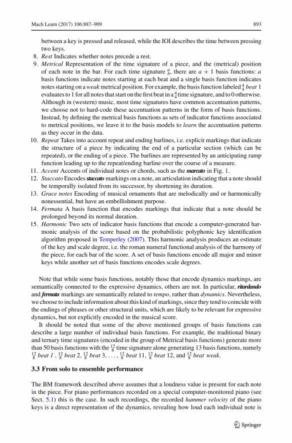
The BM framework described above assumes that a loudness value is present for each notein the piece. For piano performances recorded on a special computer-monitored piano (seeSect. 5.1) this is the case. In such recordings, the recorded hammer velocity of the pianokeys is a direct representation of the dynamics, revealing how loud each individual note is

123

894 Mach Learn (2017) 106:887–909

Fig. 2 Illustration of merging and fusion of score information of two different parts belonging to the sameinstrument class “Oboe”. The matrix on the left shows two example basis functions, ϕpitch and ϕdur, for thefirst notes of each of the two score parts. The matrix top right is the result of merging basis functions ofdifferent “Oboe” instantiations into a single set. The matrix on the bottom right is the result of fusion, appliedper basis function to each set of values occurring at the same time point

played. For acoustic instruments other than the piano, such precise recording techniques arenot available, and therefore the dynamics of music ensembles such as symphonic orchestrascannot be measured in a similar way. Another approach would be to record each instrumentof the orchestra separately, and measure the loudness variations in each of the instruments,but this approach is not feasible either, since apart from the financial and practical barriers,the live setting in which orchestras normally play prevents a clean separation of the recordingchannels by instrument. This means we are left with only a rudimentary representation ofdynamics, namely the overall variation of loudness over time, measured from the orchestralrecording.

The way dynamics is measured and represented has repercussions for the basis functionmodeling approach. In contrast to the digital grand piano setting, the overall loudness mea-sured from an orchestral recording does not provide a loudness value for each performed note,but one per time instant. Thus, basis function information describing multiple simultaneousnotes must be combined to account for a single loudness value. We do so by defining fusionoperators for subsets of basis functions. In most cases, the average operator is an adequateform of fusing basis function information. For some basis functions however, we use thesum operator, in order to preserve information about the number of instances that were fusedinto a single instrument. Future experimentation should provide more informed choices asto the optimal fusion operators to use, including the use of different weighting strategies andnonlinear aggregation of the basis functions.

Another significant changewith respect to the solo instrument setting is that in an ensemblesetting, multiple sets of basis functions are produced, each set describing the score part of aparticular instrument. In a symphonic piece, multiple instantiations of the same instrumentmay be present. Moreover, different pieces may have different instrumentations. This posesa challenge to an expression model, which should account for the influence of instrumentsconsistently fromone piece to the other.We address this issue by defining amerging operationthat combines the information of different sets of basis functions for each instance of aninstrument into a single set of basis functions per instrument class. Both the merging and thefusion operations are illustrated for a musical excerpt in Fig. 2.

The proposed description of orchestral music can easily generate a very large amountof basis functions, since each instrument has its own set of basis functions. For exam-

123

Mach Learn (2017) 106:887–909 895

ple, the metrical basis functions corresponding to the traditional binary and ternary timesignatures for the classical string section1 generate more than 250 basis functions (e.g.,Violin 3

4 beat 1, Viola 34 beat 1, etc.).

4 Linear, non-linear, and recurrent non-linear basis models

In the previous sectionwe have described how themusical scores of solo and ensemble piecescan be described bymeans of basis functions, and how expressive dynamics can bemeasured,but we have not yet described how to model the relation between expressive dynamics andthe basis functions. In this section we describe three models of increasing complexity.

In the following, X = {x1, . . . , xN } represents the set of N notes in a musical score.The values of the basis functions corresponding to note xi are denoted by a vector ϕ(xi ) =(ϕ1(xi ), . . . , ϕM (xi ))T ∈ R

M . In this way, we can represent a whole musical score as Φ ∈R

N×M , a matrix with elements Φi j = ϕ j (xi ). The values of the expressive parameters foreach note predicted by a BM model are represented by vector y = (y1, . . . , yN )T ∈ R

N . Wecan model the expressive parameters as a function of the input basis functions as

y = f (Φ;w), (1)

where f (·) is a function of Φ given parameters w.

4.1 Linear basis models (LBMs)

The simplest way to explore the influence of the basis functions in the expressive parametersis using a linear regression. The LBM models expressive dynamics of the i th note in a scorexi as a weighted sum of the basis functions as

yi = ϕ(xi )Tw, (2)

where w ∈ RM is a vector of weights.

4.2 Non-linear basis models (NBM)

The influence of the basis functions in the expressive parameter can be modeled in a non-linear way using feed forward neural networks (FFNNs). These neural networks can bedescribed as a series of (non-linear) transformations of the input data (Bishop 2006). Usingthis formalism, we can write the expressive parameter corresponding to the i th note as theoutput of a fully-connected FFNN with L hidden layers as

yi = f (L)(w(L)Th(L−1)

i + w(L)0

), (3)

where h(L−1)i ∈ R

DL−1 is the activation of the (L − 1)th hidden layer (with DL−1 units)corresponding to the i th note; f (L)(·) is an element-wise activation function and w(L) ∈R

DL−1 andw(L)0 ∈ R are the vector of weights and a scalar bias of the Lth layer, respectively.

The activation for the lth hidden layer corresponding to the i th note h(l)i ∈ R

Dl , where Dl isthe number of units in the layer, is given by

h(l)i = f (l)

(w(l)h(l−1)

i + w(l)0

), (4)

1 Violin, viola, violoncello and double bass.

123

896 Mach Learn (2017) 106:887–909

y1 y2 y3 y4 y5 y6

h(2)1 h(2)

2 h(2)3 h(2)

4 h(2)5 h(2)

6

h(1)1 h(1)

2 h(1)3 h(1)

4 h(1)5 h(1)

6

ϕ(x1) ϕ(x2) ϕ(x3) ϕ(x4) ϕ(x5) ϕ(x6)

Fig. 3 The architecture of the used NBM for modeling expressive dynamics. From bottom to top, the circlesrepresent the input layer, two successive hidden layers and the output layer, respectively. From left to right,advancing time steps are shown

where w(l) ∈ RDl×Dl−1 and w(l)

0 ∈ RDl are the matrix of weights and the bias vector

of the lth layer; and h(l−1)i ∈ R

Dl−1 is the activation of the (l − 1)th hidden layer. Theelement-wise activation function of the lth layer is represented by f (l). As a convention,the 0th layer represents the input itself, i.e. h(0)

i = ϕ(xi ). The set of all parameters is

w = {w(1)0 ,w(1), . . . , w

(L)0 ,w(L)}. Common activation functions for the hidden layers are

sigmoid, hyperbolic tangent, softmax and rectifier (ReLU (ξ) = max(0, ξ)). Since we areusing the FFNN in a regression scenario, the activation function of the last layer is set to theidentity function ( f (L)(ξ) = ξ ) (Bishop 2006).

Figure 3 schematically illustrates an NBM with 2 hidden layers.

4.3 Recurrent non-linear basis models (RNBMs)

Both the LBM and NBM models are static model that do not allow for modeling temporaldependencies within parameters. This problem can be addressed by using recurrent neuralnetworks (RNNs). The basic structure of an RNN is the recurrent layer. The output of onesuch layer at time t , can be written as

ht = fh(gϕ (ϕ(xt )) + gh (ht∗)

), (5)

where gϕ (ϕ(xt )) represents the contribution of the input of the network at time t , gh (ht∗) isthe contribution of other time steps (past or future, or a combination of both) of the state ofthe recurrent layer. As in the case of NBMs, fh(·) is an elementwise (non-linear) activationfunction. The output of the network can be computed in a similar fashion to traditionalFFNNs using Eq. (3), where the non-recurrent and recurrent hidden layers are computedusing Eqs. (4) and (5), respectively. For modeling expressive dynamics, we use BidirectionalRNNs (Schuster and Paliwal 1997). In this way, we combine information from the past andfuture score information to make a prediction of the dynamics of the current note.

While it is theoretically possible for large enough vanilla RNNs to predict sequences ofarbitrary complexity, it has been shown that numerical limitations of training algorithms donot allow them to properly model long temporal dependencies (Pascanu et al. 2013). Toaddress these problems, the Long Short Term Memory (LSTM) architecture were proposed

123

Mach Learn (2017) 106:887–909 897

y1 y2 y3 y4 y5 y6

h1;bw h2;bw h3;bw h4;bw h5;bw h6;bw

h1;fw h2;fw h3;fw h4;fw h5;fw h6;fw

ϕ(x1) ϕ(x2) ϕ(x3) ϕ(x4) ϕ(x5) ϕ(x6)

Fig. 4 Bidirectional RNBM for modeling expressive dynamics. The single hidden layer h is made up fromforward (fw) and backward (bw) recurrent hidden units. Left to right shows advancing time steps

in Hochreiter and Schmidhuber (1997). LSTMs include special purpose recurrent layers withmemory cells that allow for a better finding and exploiting long range dependencies in thedata. A more mathematical formulation of RNNs can be found in Graves (2013).

Figure 4 shows the scheme of an RNBM with a single bidirectional layer.

4.4 Learning the parameters of the model

Given T = {(Φ1, t1), . . . , (ΦK , tK )}, a set of training pairs of scores and their correspond-ing expressive targets, the parameters of the models presented above can be estimated in asupervised way by minimizing the mean squared error between predictions and targets, i.e.

w = argminw

1

K

∑k

‖ f (Φk;w) − tk‖2. (6)

4.5 A note on evaluation strategies for computational models of musicalexpression

It is important to emphasize that the mean squared error (or other derived measures) withrespect to a human performance is not necessarily a reliable indicator of the musical qualityof a generated performance. Firstly, a low error does not always imply that a performancesounds good—at crucial places, a few small errors maymake the performance sound severelyawkward, even if these error hardly affect the overall error measure. Secondly, the very notionof expressive freedom implies that music can often be performed in a variety of ways that arevery different, but equally convincing in their own right. In that sense, evaluating the modelsonly by their ability to predict the performance of a single performer is not sufficient in thelong run.

In spite of that, there are good reasons in favor of the mean squared error as a guidefor evaluating performance model. Firstly, music performance is not only about individualexpressive freedom. The works of Repp (e.g. Repp 1992, 1994) have shown that there aresubstantial commonalities in the variations of timing and dynamics across performers. Webelieve that assessing howwell the model predicts existing human performances numericallydoes tell us something about the degree to which it has captured general performance princi-

123

898 Mach Learn (2017) 106:887–909

ples. Secondly, model assessment involving human judgments of the perceptual validity ofoutput is a time-consuming and costly effort, not practicable as a recurring part of an iterativemodel development/evaluation process. For such a process, numerical benchmarking againstperformance corpora is more appropriate. Note however that anecdotal perceptual validationof the BMs has taken place on several occasions, in the form of concerts/competitions wherethe BM, along with competing models was used to perform musical pieces live in front ofan audience, on a computer-controlled grand piano.2

5 Experiments

To determine to what degree the different model types are able to account for expressivedynamics, we subject them to a comparative evaluation on different data sets. For each ofthree data sets, the accuracy of themodel predictions are tested using fivefold cross validation,where the set of instances belonging to a single musical piece was either entirely part of thetraining set, the validation set, or the test set, respectively. This is important since otherwise,repeated structures in the music that end up in different sets may cause an overly optimisticimpression of the generalizing capabilities of the models.

5.1 Data sets

Below, we describe the three different data sets used. The first two consist of classical solopiano performances, and the third of classical symphonic music.

5.1.1 Magaloff/Chopin

The Magaloff/Chopin corpus (Flossmann et al. 2010) consists of the complete Chopin pianosolo works performed by renown pianist Nikita Magaloff (1912–1992) during a series ofconcerts in Vienna, Austria in 1989. These performances were recorded using a BösendorferSE computer-monitored grand piano, and then converted into standard MIDI format.

The performances have been aligned to their corresponding machine-readable musicalscores inMusicXML format, which were obtained from hard-copies of the sheet music usingcommercial optical music recognition software3 and subsequent manual correction. Thescore-performance alignment step has also been performed semi-automatically, involvingmanual correction of automatic alignments.

The data set comprises more than 150 pieces and over 300,000 performed notes, addingup to almost 10h of music. The basis function extraction on this data produces 167 basisfunctions.

5.1.2 Zeilinger/Beethoven

This is another corpus of classical piano performances, very similar in form and modalitiesto the Magaloff/Chopin corpus. It consists of the performances of 31 different movements

2 Predecessors of the current BM approach have won awards at the 2008 and 2011 editions of the MusicPerformance Rendering Contest (Rencon) (Hashida et al. 2008), and have been evaluated favorably in a Turingtest-like concert organized as part of the 1st International Workshop on Computer and Robotic Systems forAutomatic Music Performance (SAMP14) (De Poli et al. 2015; Rodà et al. 2015).3 http://www.visiv.co.uk/.

123

Mach Learn (2017) 106:887–909 899

Table 1 Musical material contained in the RCO/Symphonic corpus

Composer Piece Movements Conductor

Beethoven Symphony no. 5 in C-Min. (op. 67) 1, 2, 3, 4 Fischer

Beethoven Symphony no. 6 in F-Maj. (op. 68) 1, 2, 3, 4, 5 Fischer

Beethoven Symphony no. 9 in D-Min. (op. 125) 1, 2, 3, 4 Fischer

Mahler Symphony no. 4 in G-Maj. 1, 2, 3, 4 Jansons

Bruckner Symphony no. 9 in D-Min. (WAB 109) 1, 2, 3 Jansons

from 9 different Beethoven Sonatas by Austrian concert pianist Clemens Zeilinger, recordedunder studio conditions at the Anton-Bruckner University in Linz (Austria), on January 3–5,2013. The pieces were performed on a Bösendorfer CEUS 290 computer-monitored grandpiano, and converted to standard MIDI format. Further preparation of the data, such as theproduction of machine-readable scores, and score to performance alignment were done in thesame way as for theMagaloff/Chopin corpus. This data set comprises over 70,000 performednotes, adding up to just over 3h of music. The basis function extraction on this data produces163 basis functions.

One of the unique properties of both the Zeilinger/Beethoven and the Magaloff/Chopincorpora is that the timing and hammer velocities of each performed note have been recordedwith precise measuring equipment directly in the piano, and are not based on manual anno-tation of audio-recordings.

5.1.3 RCO/Symphonic

The RCO/Symphonic corpus consists of symphonies from the classic and romantic period.It contains recorded performances (audio), machine-readable representations of the musicalscore (MusicXML) and automatically produced (using the method described in Grachtenet al. 2013), manually corrected alignments between score and performance, for each of thesymphonies. The manual corrections were made either at bar or at beat level (depending onthe tempo of the piece), and subsequently, the performance was re-aligned automatically,using the corrected positions as anchors.

The pieces were performed by the Royal Concertgebouw Orchestra, conducted by eitherIván Fischer orMariss Jansons, at the Royal Concertgebouw in Amsterdam, the Netherlands.The corpus amounts to a total of 20 movements from five pieces, listed in Table 1. Thecorresponding performances sum up to a total length of over 4, 5h of music. From the 20scores a total of 53,816 note onsets (post merging and fusion), and 1420 basis functions wereextracted.4

The loudness of the recordings was computed using the EBU-R 128 loudness mea-sure (EBU-R-128 2011) which is the recommended way of comparing loudness levels ofaudio content in the broadcasting industry. This measure takes into account human percep-tion, particularly the fact that signals of equal power but different frequency content are notperceived as being equally loud. To obtain instantaneous loudness values, we compute themeasure on consecutive blocks of audio, using a block size and hop size of 1024 samples,using a 44,100Hz samplerate. Through the score-performance alignment, the resulting loud-ness curve is indexed by musical time (such that we know the instantaneous loudness of the

4 A complete description of the basis functions can be found in the following technical report:http://lrn2cre8.ofai.at/expression-models/TR2016-ensemble-expression.pdf.

123

900 Mach Learn (2017) 106:887–909

recording at, say, the second beat of measure 64 in the piece), and is thus associated to thebasis function representation of the piece.

5.2 Model training

The LBM models were trained using LSMR, an iterative algorithm for solving sparse LSproblems (Fong and Saunders 2011).

All NBM and RNBM models were trained using RMSProp (Dauphin et al. 2015), amini batch variant of stochastic gradient descent that adaptively updates the learning rateby dividing the gradient by an average of its recent magnitude. In order to avoid overfitting,l2-norm weight regularization, dropout and early stopping were used. Regularization of thel2-norm encourages parameter values to shrink towards zero unless supported by the data. Ineach run of the fivefold cross-validation, 80% of the training data was used for updating theparameters and 20%was used as validation set. Early stopping was performed by monitoringthe loss function on the validation set. Dropout prevents overfitting and provides a way ofapproximately combining different neural networks efficiently by randomly removing unitsin the network, along with all its incoming and outgoing connections (Srivastava et al. 2014).

The network architectures used in this study are the following:

1. NBM (100, 20) FFNN with 2 hidden layers with 100 and 20 units, respectively.2. RNBM (20rec) vanilla bidirectional RNN with a single hidden layer with 20 units.3. RNBM (20lstm) bidirectional LSTM with a single hidden layer with 20 units.4. RNBM (100, 20rec) RNN consisting of a non-recurrent hidden layer with 100 units

followed by a vanilla bidirectional recurrent layer with 20 units.

The hidden layers of all the above described models have ReLU units. We used linearoutput layer with a single unit for all models.

The number of layers and units in the NBM (100, 20) architecture were empiricallyselected from a non-exhaustive search conducted while performing preliminary experimentson jointmodeling of expressive dynamics, timing and articulation. This searchwas performedusing fivefold cross-validations on smaller subsets of the classical piano datasets (around twothirds of the pieces for each dataset) and a larger subset of basis functions.5 The results ofthese experiments lie outside the scope of this paper and, therefore, are not reported here. TheRNBM (20rec) was previously used for modeling expressive timing in Grachten and CancinoChacón (2017). We decided to use the same architecture with the more sophisticated LSTMlayer, resulting in the RNBM (20lstm). Finally, the RNBM (100, 20rec) is a combination ofboth NBM (100, 20) and the RNBM (20rec). This architecture performs a low-dimensionalencoding of the information contained in the basis functions in its first hidden layer, whichthen is used as an input for the recurrent layer.

All NBMandRNBMmodels were trained for amaximum of 2000 epochs using a learningrate of 10−5, the probability of dropout set to 0.5 and the regularization coefficient equal to10−3. These parameters were selected empirically.

Therefore, it is important to emphasize that the results reported in this paper do notnecessarily correspond to the optimal architecture for each dataset.

5 The NBM (100, 20) architecture was neither the best for the Magaloff/Chopin dataset nor for theZeilinger/Beethoven dataset, but performed relatively well given its simplicity.

123

Mach Learn (2017) 106:887–909 901

Table 2 Predictive accuracy for expressive dynamics in terms of explained variance (R2) and Pearson’scorrelation coefficient (r ), averaged over a fivefold cross-validation on each of the three corpora

Model Magaloff/Chopin Zeilinger/Beethoven RCO/Symphonic

R2 r R2 r R2 r

LBM 0.171 0.470 0.197 0.562 −0.352 0.312

NBM (100, 20) 0.195 0.478 0.266 0.568 0.242 0.528

RNBM (20rec) 0.205 0.518

RNBM (20lstm) 0.271 0.590

RNBM (100, 20rec) 0.282 0.609

Due to the structure of the data, the RNBM models cannot be directly used to model expressive dynamics inthe Magaloff/Chopin and Zeilinger/Beethoven corpora (see text)

6 Results and discussion

In this section, we present and discuss the results of the cross-validation experiments.We firstpresent the predictive accuracies, and continue with a qualitative analysis of the results, inwhichwe use sensitivity analysismethods to revealwhat relations between the basis functionsand the expressive dynamics the LBM and NBMmodels have learned. A qualitative analysisof the recurrent models is beyond the scope of this paper. We conclude the Section with somegeneral remarks on the results.

6.1 Predictive accuracy

Table 2 shows the predictive accuracy of the LBM and the NBM Models in the fivefoldcross-validation scenario on all three corpora, and the results of the RNBM models for theRCO/Symphonic corpus. The reason for this asymmetry is that the RNBM model assumesthe data to be strictly sequential. This is the case for the RCO/Symphonic data, as a resultof the fusion operation performed on the values of the basis functions (see Sect. 3.3; Fig. 2),but not for the solo piano corpora. Since the piano recordings have MIDI velocity values pernote, rather than per time position, the data instances seen by the model also correspond tonotes. This means that simultaneous notes, as played in a chord, are processed sequentially,and violates the assumption that the data is strictly sequential in a temporal sense.

The R2 values in Table 2 quantify the proportion of variance in the target data that isexplained by the model. This quantity is defined as R2 = 1 − SSerr/SSy , where SSerr isthe sum of squared errors between the predictions and the target, and SSy is the total sum ofsquares of the target. Pearson’s correlation coefficient (r ) expresses how strongly predictionsand target are linearly correlated.

Both measures show a consistent improvement of the NBM model over the LBM model,in particular R2. This shows that the theoretical benefits of non-linear modeling (non-lineartransformations of the input, and interactions between inputs) have practical value in thecontext of modeling expressive dynamics.

Further improvements can be made by modeling temporal dependencies (as in the RNBMmodels), but the results also show that the model needs a significant capacity in order tocapture the relationship between the basis functions and expressive dynamics. In particular,RNBM (20rec) containing only 20 recurrent units performs worse than the non-recurrentNBM (100, 20) with two hidden layers of 100 and 20 units, respectively. RNBM (20lstm)does perform substantially better, but it should be noted that the LSTM units are compos-

123

902 Mach Learn (2017) 106:887–909

ite structures themselves, with additional parameters. The best observed results have beenproduced by the RNBM (100, 20rec).

Priorwork based on theMagaloff/Chopin data has revealed that amajor part of the varianceexplained by theLBMis accounted for by the basis functions that represent dynamicmarkingsand pitch, respectively, whereas other basis functions had very little effect on the predictiveaccuracy of the model (Grachten and Widmer 2012). To gain a better insight into the rolethat different basis functions play in each of the models, the learned models must be studiedin more detail. For the LBM this is straight-forward: each of the basis functions is linearlyrelated to the target using a single weight. Therefore, the magnitude of each weight is adirect measure of the impact of its corresponding basis function on the target. In a non-linearmodel such as the NBM, the weights of the model cannot be interpreted in such a straight-forward way. To accommodate for this, we use more generic sensitivity analysis methods toinvestigate the behavior of computational models.

6.2 Variance-based sensitivity analysis

In order to account for the effects of the different basis functions, a variance based sensitivityanalysis (Saltelli et al. 2010) was performed on the trained LBM and NBM models. In thissensitivity analysis, the model output y is treated as a function of the input basis functions ϕ

given the model parameters w. The sensitivity of y is explained through a decomposition ofits variance into terms depending on the input basis functions and their interactions with eachother. The first order sensitivity coefficient S1i measures the individual linear (additive) effectof the i th basis function ϕi in the model output. On the other hand, the total effect index STiaccounts for the additive effect plus all higher order effects of ϕi , including its interactionswith the rest of the basis functions. These sensitivity measures are given respectively by

S1i = Vϕi (Eϕ\ϕi (y | ϕi ))

V (y)and STi = Eϕ\ϕi

(Vϕi (y | ϕi )

)

V (y), (7)

where Vϕi is the variance with respect to the i th basis function, Eϕ\ϕi is the expected valuewith respect to all basis functions but ϕi and V (y) is the total variance of y. From thesedefinitions it is possible to show that

∑i S1i = 1 and

∑i STi ≥ 1. Furthermore, it can be

shown that for a model whose output depends linearly on its inputs, as is the case with LBMs,both S1i and STi are equal.

Both S1i and STi are estimated using a quasi-Monte Carlo method proposed by Saltelliet al. (2010). Thismethod generates a pseudo random (low-discrepancy) sequence of samplesto estimate the expected values and variances in the above equations.

Table 3 lists the basis functions that contribute the most to the variance of themodel, ordered according to S1 for the LBM models trained on Magaloff/Chopin andZeilinger/Beethoven, respectively. The columns labeled active specify the percentage ofinstances where a basis function is non-zero. This is relevant, since a high sensitivity to basisfunctions that are only very rarely active is a sign of overfitting. For this reason, we havegrayed out basis functions that are active in less than 5% of the instances.

Based on the linear model evaluated on Magaloff/Chopin it was concluded in Grachtenand Widmer (2012) that pitch and dynamics markings, are important factors for predictingexpressive dynamics. The results reported here, with amore diverse set of basis functions, andevaluated on a second corpus that is independent in terms of both performer and composer,roughly support this conclusion, since both pitch and a few of the most prominent dynamicsmarkings appear as (non-grayed-out) items in the lists. The finding that pitch is (positively)

123

Mach Learn (2017) 106:887–909 903

Table 3 Basis functions with the largest sensitivity coefficients for the LBM models

Magaloff/Chopin Zeilinger/Beethoven

Basis function Active (%) S1 Basis function Active (%) S1

pitch 100.00 0.168 sf 2.98 0.209

slur decr 63.06 0.067 smorzando 0.01 0.078

crescendo 42.71 0.067 calando 0.08 0.062

ff 39.12 0.059 crescendo 26.76 0.042

duration 100.00 0.035 ff 37.48 0.03628 beat 1 0.01 0.034 f 26.07 0.036

slur incr 62.13 0.033 fp 0.19 0.027

f 35.49 0.031 54 weak 0.01 0.026

smorzando 0.01 0.025 pitch 100.00 0.024

fff 12.86 0.023 54 beat 4 0.00 0.020

54 weak 0.12 0.022 sfp 0.06 0.018

fp 0.01 0.021 slur incr 35.92 0.018

fz 0.30 0.020 duration 100.00 0.01738 beat 1 0.07 0.020 slur decr 37.66 0.017128 beat 1 0.34 0.016 diminuendo 18.08 0.017

Averages are reported over the fivefolds of the cross-validation. Dynamics markings are in bold italic. Basisfunctions that are non-zero for less than 5% of the instances have been grayed out

correlated with expressive dynamics is in accordance both with theHigh Loud phrasing rule6

of the KTHmodel (Friberg et al. 2006), and with the unsupervised feature learning approachdescribed in Grachten and Krebs (2014).

Furthermore, the presence of the slur incr and slur decr basis functions (see Sect. 3.2)suggests that although the slur mark is strictly hint with respect to articulation, it may act as aproxy formusical grouping,which has been shown to be related to expressive dynamics (Todd1992).

Table 4 lists the bases to which the NBM model is most sensitive. Roughly speaking,the set of most important bases for the NBM model, conveys dynamics markings, pitch,slurs, and duration, as is the case of the LBM model. A notable difference is the high sen-sitivity of the NBM model to both crescendo and diminuendo markings, in both corpora. Aplausible explanation for this difference is that although crescendo/diminuendo informationin relevant for predicting expressive dynamics, the target cannot be well-approximated asa linear combination of the two basis functions. Comparing the total effect index ST andthe first order sensitivity coefficient S1 shows that the NBM model has learned interactionsinvolving diminuendo and crescendo. Although these values only indicate that diminuendo andcrescendo interact with some other bases, not necessarily with each other, in the following weshow that the latter is indeed the case.

Figure 5 shows how both the LBM and the NBMmodel behave in two different scenariosconcerning the occurrence of a crescendo. For each scenario, a score fragment is shown (takenfrom theMagaloff/Chopin corpus), that exemplifies the corresponding scenario. The left halfof the figure shows the scenario where a crescendo occurs (indicated by the ramp function in

6 See Table 1 in Friberg et al. (2006) for an overview of the rules of the KTH model.

123

904 Mach Learn (2017) 106:887–909

Table 4 Basis functions with the largest sensitivity coefficients for the NBM models

Magaloff/Chopin Zeilinger/Beethoven

Basis function Active (%) S1 ST Basis function Active (%) S1 ST

pitch 100.00 0.200 0.207 sf 2.98 0.289 0.300

crescendo 42.71 0.037 0.124 diminuendo 18.08 0.071 0.135

diminuendo 41.56 0.036 0.100 duration 100.00 0.056 0.126

slur decr 63.06 0.044 0.084 crescendo 26.76 0.046 0.096

ff 39.12 0.059 0.083 f 26.07 0.083 0.095

f 35.49 0.051 0.073 slur incr 35.92 0.046 0.080

slur incr 62.13 0.062 0.073 ff 37.48 0.052 0.068

duration 100.00 0.040 0.072 p 64.41 0.025 0.034

fff 12.86 0.016 0.028 slur decr 37.66 0.020 0.033

pp 23.18 0.006 0.020 pp 40.07 0.029 0.032

accent 1.37 0.020 0.020 pitch 100.00 0.032 0.032

fz 0.30 0.018 0.018 fp 0.19 0.013 0.014

mp 5.46 0.007 0.012 ritardando 31.09 0.005 0.010

p 41.94 0.007 0.012 fermata 0.08 0.001 0.004

tot neighbors 2.50 0.009 0.011 staccato 8.41 0.005 0.005

ppp 5.79 0.001 0.011 sfp 0.06 0.002 0.004

Averages are reported over the fivefolds of the cross-validation. Dynamics markings are in bold italic. Basisfunctions that are non-zero for less than 5% of the instances have been grayed out

the crescendo input) without the interference of a diminuendo (the diminuendo input is zero).The two graphs below the inputs depict the output of the LBMandNBMmodels, respectively,as a response to these inputs. Apart from a slight non-linearity in the response of the NBM,note that the magnitude of the responses of both model is virtually equal.7

In the same way, the right half of the figure shows the response of the models to a crescendowhen preceded by a diminuendo. Note that the basis function encodes the diminuendo by aramp from 0 to 1 over the range of the wedge sign, and stays at 1 until the next constantloudness annotation,8 such that over the range of the crescendo ramp shown in the plot, thediminuendo basis function is constant at 1.

This is a common situation, as depicted in the musical score fragment, where the musicalflow requires a brief (but not sudden) decrease in loudness. Note how the response of theNBMmodel to the crescendo in this case is much reduced, and also smoother. The response ofthe LBMmodel, which cannot respond to interactions between inputs, is equal to its responsein the first scenario.

6.3 General discussion

The experiments show that the BMmodels can be used tomodel expressive dynamics both fordifferent combinations of composers and performers in pianomusic, and for orchestral musicof different composers. A question that has not been explicitly addressed in the experimentsis to what degree a model trained on one combination of composer/performer is an accurate

7 The scale of the output is arbitrary, but has been kept constant when plotting the outputs of both the LBMand NBM, to enable visual comparison.8 This behavior is illustrated for the crescendo sign in Fig. 1.

123

Mach Learn (2017) 106:887–909 905

1

0

1

0

Diminuendobasis

Inpu

tO

utpu

t

Crescendobasis

LBM

NBM

Crescendo only(Diminuendo inactive)

1

0

1

0

Diminuendobasis

Inpu

tO

utpu

t

Crescendobasis

LBM

NBM

Crescendo following Diminuendo(Diminuendo basis function remains active)

Fig. 5 Example of the effect of the interaction of crescendo after a diminuendo for both LBM and NBMmodels

model of expressive dynamics in another combination of composer/performer. Although thisquestion is hard to answer in general, it is possible to make some general observations. Firstof all, along with musical style, also performance practice has evolved over the centuries.For example, a keyboard piece from the Baroque period is typically performed very dif-ferently than piano music from the Romantic period. Models trained on one musical styleshould therefore not be expected to generalize to other styles. Within a specific musical style,expressive styles can still vary substantially from one performer to the other. As mentionedin Sect. 4.5 however, there are substantial commonalities in the expressive dynamics acrossperformers (Repp 1992, 1994), taking the form of general performance principles. As thesensitivity analysis shows (Sect. 6.2), some of these principles are captured by the model,even if it is trained on the performances of a single performer. This suggest that at least tosome extent, within a musical style the models may generalize from one performer to theother. However, beyond the search for general performance principles, the BM approachmaybe used to characterize the individuality of celebrated performers. Preliminary work in thisdirection has been presented in Grachten et al. (2017).

7 Conclusions and future work

Expressive dynamics in classical music is a complex phenomenon, of which our understand-ing is far from complete. A variety of computational models have been proposed in the past,

123

906 Mach Learn (2017) 106:887–909

predominantly for classical pianomusic, as a way to gain a better understanding of expressivedynamics. In this paper we have extended a simple but state-of-the-art model for musicalexpression involving linear basis function modeling (Grachten and Widmer 2012), in orderto investigate whether expressive dynamics can be more accurately modeled using non-linearmethods. To that end we have carried out an extensive comparative evaluation of the linearand non-linear models, not only on different classical piano corpora, but also on a corpus ofsymphonic orchestra recordings.

The results show that non-linear methods allow for substantially more accurate modelingof expressive dynamics. A qualitative analysis of the trained models reveals that non-linearmodels effectively learn interaction-effects between aspects of the musical score that linearmodels cannot capture. Through this analysis we also find that the models reproduce severalregularities in expressive dynamics that have been individually found or hypothesized inother literature, such as that high notes should be played louder, or that musical grouping(as expressed by slur marks) is a determining factor for expressive dynamics. Thus, thecontribution of the present study is firstly that it provides evidence for these findings, whichare sometimes no more than a musical intuition or conjecture, based on two independent datasets. Secondly, we have shown that a qualitative analysis of the models can lead to musicallyrelevant insights such as the fact that a crescendo marking following a diminuendo tends toproduce a less intense loudness increase than when occurring in isolation. This regularity,although musically intuitive (to some perhaps even trivial), to the best of our knowledgehas not been formulated before. Thirdly, the models provide a unified framework in whichregularities in expressive dynamics may be represented, as opposed to models that representonly a single aspect of the expressive performance.

Furthermore, on a corpus of classical symphonic recordings we have shown that modelingtemporal dependencies, either using a standard bi-directional recurrent model or using a bi-directional LSTMmodel (Hochreiter and Schmidhuber 1997), leads to a further improvementof predictive accuracy. Although it is beyond the scope of the current paper, the temporalmodeling is a promising avenue for further investigation in musical expression. In particular,it may allow for a more parsimonious representation of musical events in the score (such asa slur being described by two instantaneous events for its start and end, respectively, ratherthan ramp functions), since the model can use information from non-contiguous future andpast events to make its current predictions.

Further prospective work is the combination of the current work with unsupervised fea-ture learning of musical score representations (using Deep Learning) (Grachten and Krebs2014; van Herwaarden et al. 2014). The benefit of this hybrid approach is that it combinesinformation about annotations in the musical score, that are not part of the representationlearning process but are definitely relevant for modeling expression, with the adaptivenessand malleability of representations learned from musical data.

As previously stated in Sect. 4.5, a model with high predictive accuracy might not nec-essarily render a good musical performance of a piece. Therefore, in addition to numericalevaluation of the model outputs, future evaluation will also involve listening tests. An inter-esting intermediate form between numerical evaluation and perceptual validation of modeloutputs is to define perceptually inspired objective functions. In the computer vision andimage processing communities there have been several efforts in this direction, includingthe definition of the structural similarity index (Wang et al. 2004). For musical expression, astarting point is the perceptual model described in Honing (2006).

One of the limitations of the variants of the BMs presented in this paper is that they do notaccount for different expressive interpretations of the same score. Future work might involveprobabilistic basis-models that can explicitly learn multi-modal predictive distributions over

123

Mach Learn (2017) 106:887–909 907

the target values. Such models are better suited to train on corpora consisting of multipleperformances of the same piece (possibly bymany different performers). A natural step in thisdirection would be the use of Mixture Density Networks (Bishop 2006; Graves 2013), whichuse the output of neural networks to parameterize a probability distribution. Additionally,these models allow for joint modeling of different expressive parameters (e.g. dynamics,timing and articulation) in a more ecological fashion.

Acknowledgements Open access funding provided by Johannes Kepler University Linz. This work is sup-ported by EuropeanUnion Seventh Framework Programme, through the Lrn2Cre8 (FETGrant Agreement No.610859) and by the European Research Council (ERC) under the EU’s Horizon 2020 Framework Programme(ERC Grant Agreement No. 670035, project CON ESPRESSIONE). We gratefully acknowledge the supportof NVIDIA Corporation with the donation of a Tesla K40 GPU that was used for this research. Special thanksto pianist Clemens Zeilinger for recording the Beethoven sonatas, and to the Bösendorfer piano company fortheir longstanding support.

Open Access This article is distributed under the terms of the Creative Commons Attribution 4.0 Interna-tional License (http://creativecommons.org/licenses/by/4.0/), which permits unrestricted use, distribution, andreproduction in any medium, provided you give appropriate credit to the original author(s) and the source,provide a link to the Creative Commons license, and indicate if changes were made.

References

Bishop, C. M. (2006). Pattern recognition and machine learning. New York, NY: Springer Science.Bishop, L., Bailes, F., & Dean, R. T. (2014). Performing musical dynamics. Music Perception, 32(1), 51–66.Bresin, R. (1998). Artificial neural networks based models for automatic performance of musical scores.

Journal of New Music Research, 27(3), 239–270.Cancino Chacón, C. E., Grachten, M., & Widmer, G. (2014). Bayesian linear basis models with gaussian

priors for musical expression. Technical report. Austrian Research Institute for Artificial Intelligence,Vienna, TR-2014-12.

Clarke, E. F. (1988). Generative principles in music. In J. Sloboda (Ed.), Generative processes in music: Thepsychology of performance, improvisation, and composition. Oxford: Oxford University Press.

Dauphin, Y. N., de Vries, H., Chung, J., & Bengio, Y. (2015). RMSProp and equilibrated adaptive learningrates for non-convex optimization. arXiv:1502.4390.

De Poli, G., Canazza, S., Rodà, A., & Schubert, E. (2015). The role of individual difference in judgingexpressiveness of computer-assisted music performances by experts. ACM Transactions on AppliedPerception, 11(4), 1–20.

De Poli, G., Canazza, S., Rodà, A., Vidolin, A., & Zanon, P. (2001). Analysis and modeling of expressiveintentions in music performance. In Proceedings of the international workshop on human supervisionand control in engineering and music. Kassel, Germany.

EBU-R-128. (2011). BU Tech 3341-2011, Practical Guidelines for Production and Implementation in Accor-dance with EBU R 128. https://tech.ebu.ch/docs/tech/tech3341.pdf.

Flossmann, S., Goebl, W., Grachten, M., Niedermayer, B., & Widmer, G. (2010). The Magaloff project: Aninterim report. Journal of New Music Research, 39(4), 363–377.

Fong, D. C. L., & Saunders, M. (2011). LSMR: An iterative algorithm for sparse least-squares problems. SIAMJournal on Scientific Computing, 33(5), 2950–2971.

Friberg, A., Bresin, R., & Sundberg, J. (2006). Overview of the KTH rule system for musical performance.Advances in Cognitive Psychology, 2(2–3), 145–161.

Friberg, A., & Sundberg, J. (1999). Does music performance allude to locomotion? Amodel of final ritardandiderived from measurements of stopping runners. Journal of the Acoustical Society of America, 105(3),1469–1484.

Gabrielsson, A. (2003). Music performance research at the millennium. The Psychology of Music, 31(3),221–272.

Gadermaier, T., Grachten, M., & Cancino Chacón, C. E. (2016). Modeling loudness variations in ensembleperformance. In Proceedings of the 2nd international conference on new music concepts (ICNMC 2016).ABEditore, Treviso, Italy.

Goebl, W. (2001). Melody lead in piano performance: Expressive device or artifact? Journal of the AcousticalSociety of America, 110(1), 563–572.

123

908 Mach Learn (2017) 106:887–909

Grachten, M., & Cancino Chacón, C. E. (2017). Temporal dependencies in the expressive timing of classicalpiano performances. In M. Lesaffre, M. Leman, & P. J. Maes (Eds.), The Routledge companion ofembodied music interaction (pp. 362–371).

Grachten, M., Cancino Chacón, C. E., Gadermaier, T., & Widmer, G. (2017). Towards computer-assistedunderstanding of dynamics in symphonic music. IEEE Multimedia, 24(1), 36–46.

Grachten, M., Cancino Chacón, C. E., & Widmer, G. (2014). Analysis and prediction of expressive dynamicsusing Bayesian linear models. In Proceedings of the 1st international workshop on computer and roboticsystems for automatic music performance (pp. 545–552).

Grachten, M., Gasser, M., Arzt, A., & Widmer, G. (2013). Automatic alignment of music performances withstructural differences. In Proceedings of the 14th international society for music information retrievalconference, Curitiba, Brazil.

Grachten, M., & Krebs, F. (2014). An assessment of learned score features for modeling expressive dynamicsin music. IEEE Transactions on Multimedia, 16(5), 1211–1218. doi:10.1109/TMM.2014.2311013.

Grachten, M., & Widmer, G. (2012). Linear basis models for prediction and analysis of musical expression.Journal of New Music Research, 41(4), 311–322.

Graves, A. (2013). Generating sequences with recurrent neural networks. arXiv:1308.0850.Grindlay, G., & Helmbold, D. (2006). Modeling, analyzing, and synthesizing expressive piano performance

with graphical models. Machine Learning, 65(2–3), 361–387.Hashida, M., Nakra, T., Katayose, H., Murao, T., Hirata, K., Suzuki, K., & Kitahara, T. (2008). Rencon:

Performance rendering contest for automated music systems. In Proceedings of the 10th internationalconference on music perception and cognition (ICMPC), Sapporo, Japan.

Hochreiter, S., & Schmidhuber, J. (1997). Long short-term memory. Neural Computation, 9(8), 1735–1780.Honing, H. (2006). Computational modeling of music cognition: A case study on model selection. Music

Perception, 23(5), 365–376.Juslin, P. (2001). Communicating emotion in music performance: A review and a theoretical framework. In P.

Juslin & J. Sloboda (Eds.),Music and emotion: Theory and research (pp. 309–337). New York: OxfordUniversity Press.

Palmer, C. (1996). Anatomy of a performance: Sources of musical expression.Music Perception, 13(3), 433–453.

Palmer, C. (1997). Music performance. Annual Review of Psychology, 48, 115–138.Pascanu, R., Mikolov, T., & Bengio, Y. (2013). On the difficulty of training recurrent neural networks. In

Proceedings of the 30th international conference on machine learning, Atlanta, GA, USA (pp. 1–9).Ramirez, R., & Hazan, A. (2004). Rule induction for expressive music performance modeling. In ECML

workshop advances in inductive rule learning.Repp, B. H. (1992). Diversity and commonality in music performance—An analysis of timing microstructure

in Schumann’s “Träumerei”. Journal of the Acoustical Society of America, 92(5), 2546–2568.Repp, B. H. (1994). Relational invariance of expressive microstructure across global tempo changes in music

performance: An exploratory study. Psychological Research, 56, 285–292.Repp, B. H., London, J., & Keller, P. E. (2013). Systematic distortions inmusicians’ reproduction of cyclic

three-intervalrhythms. Music Perception: An Interdisciplinary Journal, 30(3), 291–305. doi:10.1525/mp.2012.30.3.291. http://mp.ucpress.edu/content/30/3/291.

Rodà, A., Schubert, E., De Poli, G., & Canazza, S. (2015). Toward a musical Turing test for automatic musicperformance. In International symposium on computer music multidisciplinary research.

Saltelli, A., Annoni, P., Azzini, I., Campolongo, F., Ratto, M., & Tarantola, S. (2010). Variance based sensi-tivity analysis of model output. Design and estimator for the total sensitivity index. Computer PhysicsCommunications, 181(2), 259–270.

Schuster, M., & Paliwal, K. K. (1997). Bidirectional recurrent neural networks. IEEE Transactions on SignalProcessing, 45(11), 2673–2681.

Sloboda, J. A. (1983). The communication of musical metre in piano performance. Quarterly Journal ofExperimental Psychology, 35A, 377–396.

Srivastava, N., Hinton, G., Krizhevsky, A., Sutskever, I., & Salakhutdinov, R. (2014). Dropout: A simple wayto prevent neural networks from overfitting. Journal of Machine Learning Research, 15, 1929–1958.

Temperley, D. (2007). Music and probability. Cambridge, MA: MIT Press.Teramura, K., Okuma, H., Taniguchi, Y., Makimoto, S., & Maeda, S. (2008). Gaussian process regression for

rendering music performance. In Proceedings of the 10th international conference on music perceptionand cognition (ICMPC 10), Sapporo, Japan.

Timmers, R., Ashley, R., Desain, P., Honing, H., & Windsor, L. (2002). Timing of ornaments in the theme ofBeethoven’s Paisiello Variations: Empirical data and a model. Music Perception, 20(1), 3–33.

Todd, N. (1992). The dynamics of dynamics: Amodel of musical expression. Journal of the Acoustical Societyof America, 91, 3540–3550.

123

Mach Learn (2017) 106:887–909 909

van Herwaarden, S., Grachten, M., & de Haas, W. B. (2014). Predicting expressive dynamics using neuralnetworks. In Proceedings of the 15th conference of the international society for music informationretrieval (pp. 47–52).

Wang, Z., Bovik, A. C., Sheikh, H. R., & Simoncelli, E. P. (2004). Image quality assessment: From errorvisibility to structural similarity. IEEE Transactions on Image Processing, 13(4), 600–612.

Widmer, G. (2002). Machine discoveries: A few simple, robust local expression principles. Journal of NewMusic Research, 31(1), 37–50.

Widmer, G. (2003). Discovering simple rules in complex data: Ameta-learning algorithm and some surprisingmusical discoveries. Artificial Intelligence, 146(2), 129–148.

Widmer, G., & Goebl, W. (2004). Computational models of expressive music performance: The state of theart. Journal of New Music Research, 33(3), 203–216. doi:10.1080/0929821042000317804.

Windsor, W. L., & Clarke, E. F. (1997). Expressive timing and dynamics in real and artificial musical perfor-mances: Using an algorithm as an analytical tool. Music Perception, 15(2), 127–152.

123