Available online at www.sciencedirect.com

ScienceDirect

Comput. Methods Appl. Mech. Engrg. 287 (2015) 90–111www.elsevier.com/locate/cma

An enhanced AMLS method and its performance

Jin-Gyun Kima, Seung-Hwan Boob, Phill-Seung Leeb,∗

a Korea Institute of Machinery and Materials, 156, Gajeongbuk-ro, Yuseong-gu, Daejeon 305-343, Republic of Koreab Division of Ocean Systems Engineering, Korea Advanced Institute of Science and Technology, 291 Daehak-ro, Yuseong-gu, Daejeon, 305-701,

Republic of Korea

Received 4 July 2014; received in revised form 2 December 2014; accepted 6 January 2015Available online 13 January 2015

Abstract

In this paper, we present an effective new component mode synthesis (CMS) method based on the concept of the automatedmulti-level substructuring (AMLS) method. Herein, the original transformation matrix of the AMLS method is enhanced byconsidering the residual mode effect, and the resulting unknown eigenvalue in the formulation is approximated by employingthe idea of the improved reduced system (IRS) method. Using the newly defined transformation matrix, we develop an enhancedAMLS method by which original finite element (FE) models can be more precisely approximated by reduced models, and theirsolution accuracy is significantly improved. The formulation details of the enhanced AMLS method is presented, and its accuracyand computational cost is investigated through numerical examples.c⃝ 2015 Elsevier B.V. All rights reserved.

Keywords: Structural dynamics; Finite element method; Model reduction; Component mode synthesis; Dynamic substructuring; AMLS method

1. Introduction

While computation capability has increased rapidly, the demand for large scale finite element (FE) models hasincreased even more rapidly. Therefore, it has always been an important issue to reduce computational cost. A varietyof model reduction methods have been developed and widely used in many engineering fields [1–12]. The focus inmodel reduction is on reducing computational cost with the least possible loss in accuracy.

Within the structural dynamics community, component mode synthesis (CMS) is a popular and effective finiteelement (FE) model reduction method [5–12]. In CMS methods, an original (global) FE model is partitioned intosmaller substructures, substructural eigenvalue problems are solved, and a reduced model constructed by retainingonly dominant substructural modes is used for calculations, instead of the much larger original FE model. For thisreason, CMS methods can significantly reduce overall computational cost required for many applications (e.g., con-troller design for multi-body dynamics systems, structural health monitoring, structural design optimization, modelidentification).

∗ Corresponding author.E-mail address: phillseung@kaist.edu (P.-S. Lee).

http://dx.doi.org/10.1016/j.cma.2015.01.0040045-7825/ c⃝ 2015 Elsevier B.V. All rights reserved.

J.-G. Kim et al. / Comput. Methods Appl. Mech. Engrg. 287 (2015) 90–111 91

In the 1990s, the automated multi-level substructuring (AMLS) method, a computer-aided CMS method, was pro-posed in the field of applied mathematics [13–16]. Due to its computational efficiency, involving recursive partitioningand matrix reordering processes, the AMLS method has become popular for reduced-order modeling. Recently, Ben-nighof and Lehoucq [17] proposed a well-defined formulation of the AMLS method based on the concept of theCraig–Bampton (CB) method [6,17]. The AMLS method has been also used as a solver of eigenvalue problems inmany commercial FE software.

In the original CB and AMLS methods, a transformation matrix is constructed by retaining only dominant sub-structural modes. Using the transformation matrix, original FE models can be transformed into reduced models, whichapproximate the original models. With this procedure, residual substructural modes are simply truncated without fur-ther consideration. However, when the residual mode effect is considered, the accuracy of the original transformationmatrix can be improved. That is, the original (global) models can be more precisely approximated. This approachhas been used for flexibility based CMS methods, in which, unlike for the CB and AMLS methods, substructures areconnected with a free interface [7,10–12].

In this study, we derive a new transformation matrix for the AMLS method enhanced by considering the residualmode effect. One difficulty is the fact that the enhanced transformation matrix contains an unknown eigenvalue. Inorder to approximate the unknown eigenvalue, we adopt O’Callahan’s idea, which was originally proposed to developthe improved reduced system (IRS) method by improving Guyan reduction [18]. Finally, the enhanced transformationmatrix is defined without the unknown eigenvalue, and by using the newly defined transformation matrix, an enhancedAMLS method is proposed. The reduced FE models obtained from the enhanced AMLS methods have the same sizeas those obtained from the original AMLS method. However, compared to the original AMLS method, the enhancedAMLS method can provide significantly improved reduced-order models.

In the following sections, we present the general framework of CMS methods in Section 2, and briefly reviewthe original AMLS method in Section 3. In Section 4, the formulation details of the enhanced AMLS method arepresented, and its performance and computational cost are tested in Sections 5 and 6, respectively. The conclusionsare given in Section 7.

2. Component mode synthesis

In this section, the general framework of component mode synthesis (CMS) is briefly presented. In structuraldynamics, the linear dynamics equations of a global (non-partitioned) FE model can be expressed as

Mg ug + Kgug = fg, (1)

where Mg and Kg are the global mass and stiffness matrices, respectively, and ug and fg are the global displacementand force vectors, respectively. Subscript g denotes the global structure.

Considering a free harmonic vibration (fg = 0), from Eq. (1), the following eigenvalue problem of the globalmodel is obtained

Kg(ϕg)i = λi Mg(ϕg)i , i = 1, 2, . . . , Ng, with ug = 8gqg, (2)

in which λi and (ϕg)i are the global eigenvalue and eigenvector, respectively, and 8g and qg are the global eigenvec-tor matrix and its generalized coordinate vector, respectively. Ng is the number of DOFs in the global structure. Notethat λi is the square of the i th natural frequency (ωi ).

In CMS methods, the global structure is partitioned into substructures as shown in Fig. 1(a), and the eigenvalueanalyses of individual substructures are carried out to obtain the dominant substructural modes. Using the dominantsubstructural modes, the global mass and stiffness matrices in Eq. (2) can be approximated using reduced mass andstiffness matrices.

The eigenvalue problem of the reduced model (reduced eigenvalue problem) is defined as

Kp(ϕp)i = λi Mp(ϕp)i , i = 1, 2, . . . , Np, with ηp = 8pqp, (3)

where Mp and Kp are the reduced mass and stiffness matrices, respectively, and λi and (ϕp)i are the approximatedeigenvalue and eigenvector, respectively. The approximated eigenvector matrix 8p and its generalized coordinatevector qp are used to define the approximated global displacement vector ηp. The subscript p denotes the partitioned

92 J.-G. Kim et al. / Comput. Methods Appl. Mech. Engrg. 287 (2015) 90–111

a b

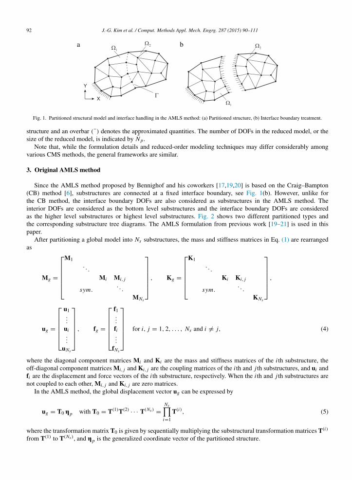
Fig. 1. Partitioned structural model and interface handling in the AMLS method: (a) Partitioned structure, (b) Interface boundary treatment.

structure and an overbar (¯) denotes the approximated quantities. The number of DOFs in the reduced model, or thesize of the reduced model, is indicated by Np.

Note that, while the formulation details and reduced-order modeling techniques may differ considerably amongvarious CMS methods, the general frameworks are similar.

3. Original AMLS method

Since the AMLS method proposed by Bennighof and his coworkers [17,19,20] is based on the Craig–Bampton(CB) method [6], substructures are connected at a fixed interface boundary, see Fig. 1(b). However, unlike forthe CB method, the interface boundary DOFs are also considered as substructures in the AMLS method. Theinterior DOFs are considered as the bottom level substructures and the interface boundary DOFs are consideredas the higher level substructures or highest level substructures. Fig. 2 shows two different partitioned types andthe corresponding substructure tree diagrams. The AMLS formulation from previous work [19–21] is used in thispaper.

After partitioning a global model into Ns substructures, the mass and stiffness matrices in Eq. (1) are rearrangedas

Mg =

M1

. . .

Mi Mi, j

sym.. . .

MNs

, Kg =

K1

. . .

Ki Ki, j

sym.. . .

KNs

,

ug =

u1...

ui...

uNs

, fg =

f1...

fi...

fNs

for i, j = 1, 2, . . . , Ns and i = j, (4)

where the diagonal component matrices Mi and Ki are the mass and stiffness matrices of the i th substructure, theoff-diagonal component matrices Mi, j and Ki, j are the coupling matrices of the i th and j th substructures, and ui andfi are the displacement and force vectors of the i th substructure, respectively. When the i th and j th substructures arenot coupled to each other, Mi, j and Ki, j are zero matrices.

In the AMLS method, the global displacement vector ug can be expressed by

ug = T0 ηp with T0 = T(1)T(2)· · · T(Ns ) =

Nsi=1

T(i), (5)

where the transformation matrix T0 is given by sequentially multiplying the substructural transformation matrices T(i)

from T(1) to T(Ns ), and ηp is the generalized coordinate vector of the partitioned structure.

J.-G. Kim et al. / Comput. Methods Appl. Mech. Engrg. 287 (2015) 90–111 93

a

b

Fig. 2. Substructure tree diagram: (a) Substructural levels 0 and 1, (b) Substructural levels 0, 1 and 2.

Due to the recursive transformation procedures in the AMLS method, the i th incompletely transformed mass andstiffness matrices, M(i ) and K(i), are defined by

M(i )=

T(1)T(2)

· · · T(i) T

Mg

T(1)T(2)

· · · T(i)

and

K(i)=

T(1)T(2)

· · · T(i) T

Kg

T(1)T(2)

· · · T(i)

, for i = 1, 2, . . . , Ns − 1.

(6)

In Eq. (6), T(i) is given by

T(i)=

I 0 0

0 8i 9 i,i+1 · · · 9 i, j · · · 9 i,Ns

0 0 I

, 8i =

8di 8r

i

,

9 i, j = −(K(i−1)i )−1 (K(i−1)

i, j ) with K(0)1, j = K1, j , for i = 1, 2, . . . , Ns and j = i + 1, i + 2, . . . , Ns, (7)

in which 8i and 9 i, j are the eigenvector matrix of the i th substructure and the constraint mode matrix to couple the

i th and j th substructures, respectively, and K(i−1)i and K(i−1)

i, j are the diagonal and off-diagonal component stiffness

matrices of the i th substructure in the (i − 1)th incompletely transformed stiffness matrix K(i−1) defined in Eq. (6).When the i th and j th substructures are not coupled to each other, 9 i, j is a zero matrix.

It is important to note that the eigenvector matrix 8i in Eq. (7) contains the dominant term 8di and the residual

term 8ri . The superscripts d and r denote the dominant and residual terms, respectively.

The eigenvector matrix 8i in Eq. (7) is calculated after solving the following substructural eigenvalue problems

K(i−1)i 8i = 3i M(i−1)

i 8i with K(0)1 = K1, M(0)

1 = M1 for i = 1, 2, . . . , Ns, (8)

where 3i is the eigenvalue matrix for the i th substructure, and M(i−1)i is the diagonal component mass matrix of

M(i−1) defined in Eq. (6). It should be noted that, to obtain the i th eigenvector matrix 8i , the (i − 1)th incompletelytransformed mass and stiffness matrices are used.

94 J.-G. Kim et al. / Comput. Methods Appl. Mech. Engrg. 287 (2015) 90–111

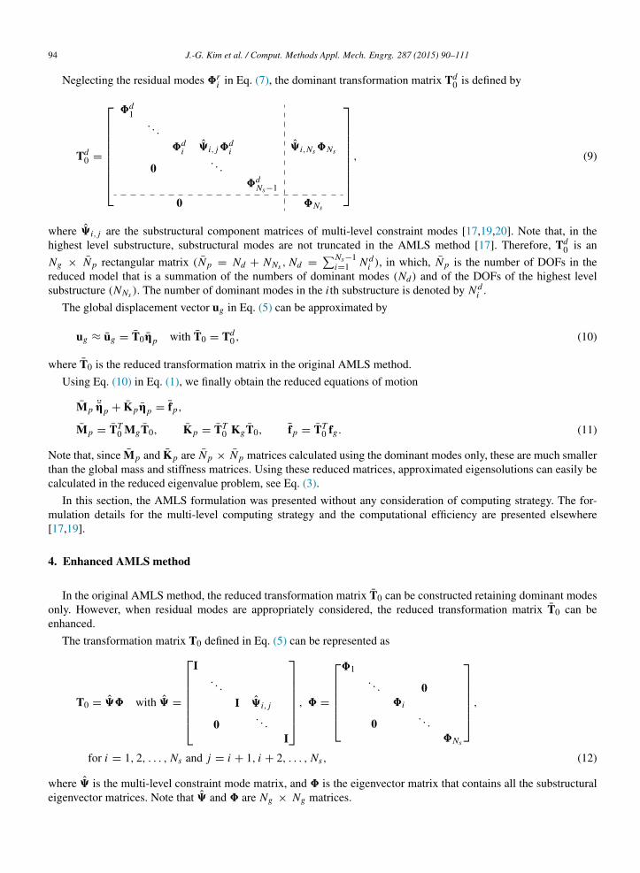
Neglecting the residual modes 8ri in Eq. (7), the dominant transformation matrix Td

0 is defined by

Td0 =

8d1

. . .

8di 9 i, j8

di 9 i,Ns 8Ns

0. . .

8dNs−1

0 8Ns

, (9)

where 9 i, j are the substructural component matrices of multi-level constraint modes [17,19,20]. Note that, in thehighest level substructure, substructural modes are not truncated in the AMLS method [17]. Therefore, Td

0 is an

Ng × Np rectangular matrix (Np = Nd + NNs , Nd =Ns−1

i=1 N di ), in which, Np is the number of DOFs in the

reduced model that is a summation of the numbers of dominant modes (Nd) and of the DOFs of the highest levelsubstructure (NNs ). The number of dominant modes in the i th substructure is denoted by N d

i .

The global displacement vector ug in Eq. (5) can be approximated by

ug ≈ ug = T0ηp with T0 = Td0 , (10)

where T0 is the reduced transformation matrix in the original AMLS method.

Using Eq. (10) in Eq. (1), we finally obtain the reduced equations of motion

Mp ¨ηp + Kpηp = fp,

Mp = TT0 MgT0, Kp = TT

0 KgT0, fp = TT0 fg. (11)

Note that, since Mp and Kp are Np × Np matrices calculated using the dominant modes only, these are much smallerthan the global mass and stiffness matrices. Using these reduced matrices, approximated eigensolutions can easily becalculated in the reduced eigenvalue problem, see Eq. (3).

In this section, the AMLS formulation was presented without any consideration of computing strategy. The for-mulation details for the multi-level computing strategy and the computational efficiency are presented elsewhere[17,19].

4. Enhanced AMLS method

In the original AMLS method, the reduced transformation matrix T0 can be constructed retaining dominant modesonly. However, when residual modes are appropriately considered, the reduced transformation matrix T0 can beenhanced.

The transformation matrix T0 defined in Eq. (5) can be represented as

T0 = 98 with 9 =

I. . .

I 9 i, j

0. . .

I

, 8 =

81

. . . 08i

0. . .

8Ns

,

for i = 1, 2, . . . , Ns and j = i + 1, i + 2, . . . , Ns, (12)

where 9 is the multi-level constraint mode matrix, and 8 is the eigenvector matrix that contains all the substructuraleigenvector matrices. Note that 9 and 8 are Ng × Ng matrices.

J.-G. Kim et al. / Comput. Methods Appl. Mech. Engrg. 287 (2015) 90–111 95

The multi-level constraint mode matrix 9 is given by sequentially multiplying the substructural constraint modematrices 9(i)

9 =

Ns−1i=1

9(i) with 9(i)=

I 0 0

0 I 9 i,i+1 · · · 9 i, j · · · 9 i,Ns

0 0 I

,

for i = 1, 2, . . . , Ns − 1 and j = i + 1, i + 2, . . . , Ns, (13)

in which 9(i) is Ng × Ng matrix. Note that 9(i) looks similar to T(i) in Eq. (7), except for the identity matrix in itsi th diagonal component.

In Eq. (12), the substructural eigenvector matrices 8i in the eigenvector matrix 8 can be represented by

8 =

[8d1 8r

1]

. . . 0[8d

i 8ri ] 0

. . .

0 [8dNs−1 8r

Ns−1]

0 8Ns

, (14)

in which 8di and 8r

i contain the dominant and residual modes in the i th substructure, respectively.

After reordering the eigenvector matrix 8 in Eq. (14), the reordered matrix 8 can be decomposed into dominantand residual parts

8 = [8d 8r ] with

8d =

8d1

8d2 0

. . .

8dNs−2

0 8dNs−1

8Ns

, 8r =

8r1

8r2 0

. . .

0 8rNs−2

8rNs−1

0

, (15)

in which 8d and 8r are the eigenvector matrices corresponding to dominant and residual substructural modes, re-spectively; 8d and 8r are Ng × Np and Ng × Nr matrices, respectively, in which the total number of residual modesNr =

Ns−1i=1 N r

i and N ri is the number of residual modes in the i th substructure.

Using Eq. (15) in Eq. (12), the global displacement vector ug in Eq. (5) can be rewritten as

ug = T0ηp =Td

0 Tr0

ηd

pηr

p

with Td

0 = 9 8d , Tr0 = 9 8r . (16)

Substituting Eq. (16) into Eq. (1) and considering a free harmonic vibration (fg = 0), we can obtain the followingequations

Kp − λMpηp = 0, (17a)

Mp = (T0)T Mg (T0), Kp = (T0)

T Kg (T0), (17b)

Kp − λMp =

3d −λMdr

−λMTdr 3r

, (17c)

96 J.-G. Kim et al. / Comput. Methods Appl. Mech. Engrg. 287 (2015) 90–111

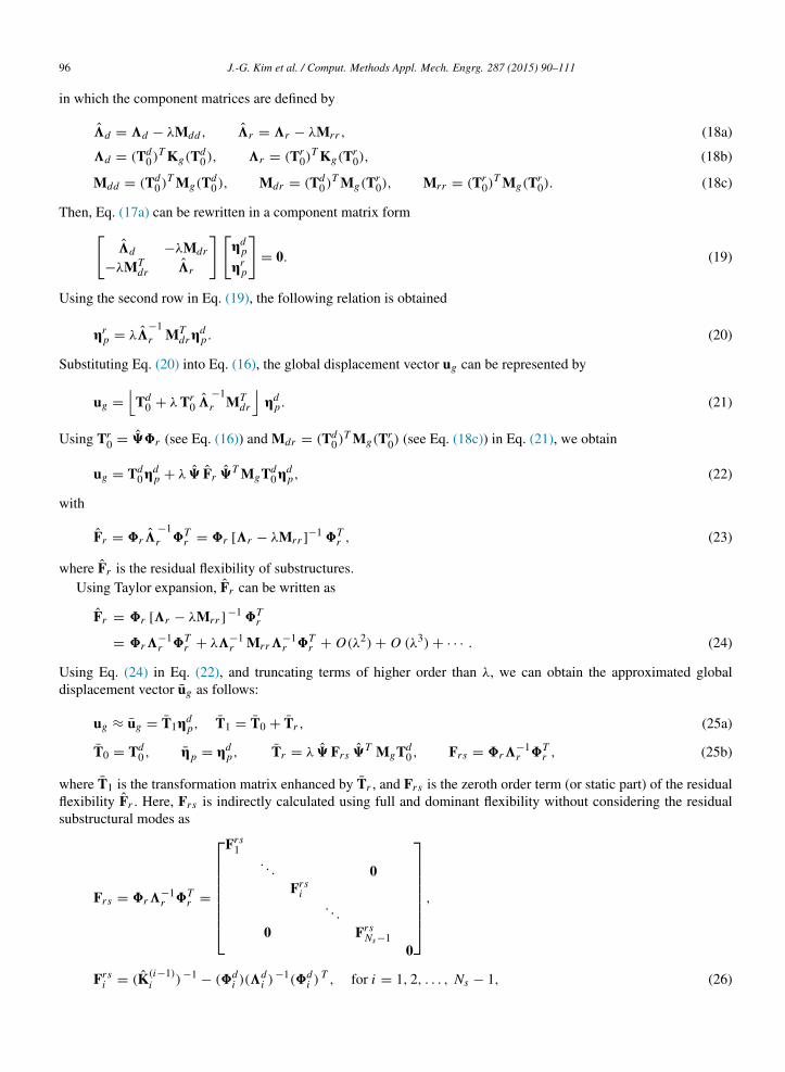
in which the component matrices are defined by

3d = 3d − λMdd , 3r = 3r − λMrr , (18a)

3d = (Td0)T Kg(Td

0), 3r = (Tr0)

T Kg(Tr0), (18b)

Mdd = (Td0)T Mg(Td

0), Mdr = (Td0)T Mg(Tr

0), Mrr = (Tr0)

T Mg(Tr0). (18c)

Then, Eq. (17a) can be rewritten in a component matrix form3d −λMdr

−λMTdr 3r

ηd

p

ηrp

= 0. (19)

Using the second row in Eq. (19), the following relation is obtained

ηrp = λ3

−1r MT

drηdp. (20)

Substituting Eq. (20) into Eq. (16), the global displacement vector ug can be represented by

ug =

Td

0 + λ Tr0 3

−1r MT

dr

ηd

p. (21)

Using Tr0 = 98r (see Eq. (16)) and Mdr = (Td

0)T Mg(Tr0) (see Eq. (18c)) in Eq. (21), we obtain

ug = Td0η

dp + λ 9 Fr 9T MgTd

0ηdp, (22)

with

Fr = 8r 3−1r 8T

r = 8r [3r − λMrr ]−1 8Tr , (23)

where Fr is the residual flexibility of substructures.Using Taylor expansion, Fr can be written as

Fr = 8r [3r − λMrr ] −1 8Tr

= 8r3−1r 8T

r + λ3−1r Mrr3

−1r 8T

r + O(λ2) + O (λ3) + · · · . (24)

Using Eq. (24) in Eq. (22), and truncating terms of higher order than λ, we can obtain the approximated globaldisplacement vector ug as follows:

ug ≈ ug = T1ηdp, T1 = T0 + Tr , (25a)

T0 = Td0 , ηp = ηd

p, Tr = λ 9 Frs 9T MgTd0 , Frs = 8r3

−1r 8T

r , (25b)

where T1 is the transformation matrix enhanced by Tr , and Frs is the zeroth order term (or static part) of the residualflexibility Fr . Here, Frs is indirectly calculated using full and dominant flexibility without considering the residualsubstructural modes as

Frs = 8r3−1r 8T

r =

Frs1

. . . 0Frs

i. . .

0 FrsNs−1

0

,

Frsi = (K(i−1)

i )−1− (8d

i )(3di )−1(8d

i ) T , for i = 1, 2, . . . , Ns − 1, (26)

J.-G. Kim et al. / Comput. Methods Appl. Mech. Engrg. 287 (2015) 90–111 97

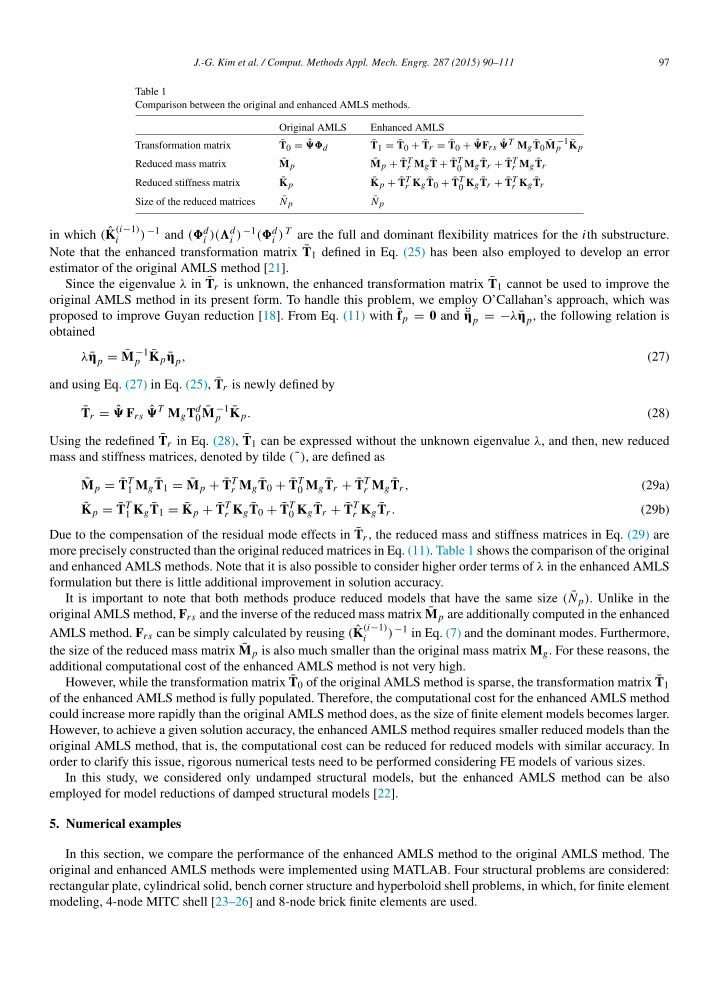
Table 1Comparison between the original and enhanced AMLS methods.

Original AMLS Enhanced AMLS

Transformation matrix T0 = 98d T1 = T0 + Tr = T0 + 9Frs 9T MgT0M −1p Kp

Reduced mass matrix Mp Mp + TTr MgT + TT

0 MgTr + TTr MgTr

Reduced stiffness matrix Kp Kp + TTr KgT0 + TT

0 KgTr + TTr KgTr

Size of the reduced matrices Np Np

in which (K(i−1)i )−1 and (8d

i )(3di )−1(8d

i ) T are the full and dominant flexibility matrices for the i th substructure.Note that the enhanced transformation matrix T1 defined in Eq. (25) has been also employed to develop an errorestimator of the original AMLS method [21].

Since the eigenvalue λ in Tr is unknown, the enhanced transformation matrix T1 cannot be used to improve theoriginal AMLS method in its present form. To handle this problem, we employ O’Callahan’s approach, which wasproposed to improve Guyan reduction [18]. From Eq. (11) with fp = 0 and ¨ηp = −ληp, the following relation isobtained

ληp = M −1p Kpηp, (27)

and using Eq. (27) in Eq. (25), Tr is newly defined by

Tr = 9 Frs 9T MgTd0M −1

p Kp. (28)

Using the redefined Tr in Eq. (28), T1 can be expressed without the unknown eigenvalue λ, and then, new reducedmass and stiffness matrices, denoted by tilde (˜), are defined as

Mp = TT1 MgT1 = Mp + TT

r MgT0 + TT0 MgTr + TT

r MgTr , (29a)

Kp = TT1 KgT1 = Kp + TT

r KgT0 + TT0 KgTr + TT

r KgTr . (29b)

Due to the compensation of the residual mode effects in Tr , the reduced mass and stiffness matrices in Eq. (29) aremore precisely constructed than the original reduced matrices in Eq. (11). Table 1 shows the comparison of the originaland enhanced AMLS methods. Note that it is also possible to consider higher order terms of λ in the enhanced AMLSformulation but there is little additional improvement in solution accuracy.

It is important to note that both methods produce reduced models that have the same size (Np). Unlike in theoriginal AMLS method, Frs and the inverse of the reduced mass matrix Mp are additionally computed in the enhanced

AMLS method. Frs can be simply calculated by reusing (K(i−1)i )−1 in Eq. (7) and the dominant modes. Furthermore,

the size of the reduced mass matrix Mp is also much smaller than the original mass matrix Mg . For these reasons, theadditional computational cost of the enhanced AMLS method is not very high.

However, while the transformation matrix T0 of the original AMLS method is sparse, the transformation matrix T1of the enhanced AMLS method is fully populated. Therefore, the computational cost for the enhanced AMLS methodcould increase more rapidly than the original AMLS method does, as the size of finite element models becomes larger.However, to achieve a given solution accuracy, the enhanced AMLS method requires smaller reduced models than theoriginal AMLS method, that is, the computational cost can be reduced for reduced models with similar accuracy. Inorder to clarify this issue, rigorous numerical tests need to be performed considering FE models of various sizes.

In this study, we considered only undamped structural models, but the enhanced AMLS method can be alsoemployed for model reductions of damped structural models [22].

5. Numerical examples

In this section, we compare the performance of the enhanced AMLS method to the original AMLS method. Theoriginal and enhanced AMLS methods were implemented using MATLAB. Four structural problems are considered:rectangular plate, cylindrical solid, bench corner structure and hyperboloid shell problems, in which, for finite elementmodeling, 4-node MITC shell [23–26] and 8-node brick finite elements are used.

98 J.-G. Kim et al. / Comput. Methods Appl. Mech. Engrg. 287 (2015) 90–111

a

b

Fig. 3. Rectangular plate problem: (a) Partition Type A, (b) Partition Type B.

The frequency cut-off mode selection method is used to select the dominant modes, and the following relativeeigenvalue error is used to measure the accuracy of the original and enhanced AMLS methods.

ξi =λ i− λi

λi, (30)

in which ξi denotes the relative eigenvalue error for the i th mode and the exact global eigenvalue λi is obtained fromthe eigenvalue problem of the global structure in Eq. (2). In the following numerical examples, rigid body modes arenot considered for the relative eigenvalue error.

5.1. Rectangular plate problem

We here consider a rectangular plate with free boundary as shown in Fig. 3. Length L is 20.0 m, width B is 12.0m, and thickness h is 0.08 m. Young’s modulus E is 206 GPa, Poisson’s ratio υ is 0.33, density ρ is 7850 kg/m3. Theplate is modeled by a 20 × 12 mesh of the 4-node MITC shell finite elements and the number of total DOFs for thisproblem is 1365. Two different partition types are considered as in Figs. 3(a) and (b):

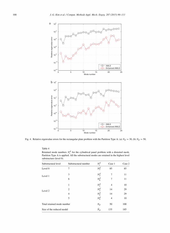
• Partition Type A: The global structure is partitioned into seven substructures with three substructural levels (levels0, 1 and 2), see Fig. 3(a). Retaining 30 and 50 dominant modes (Nd = 30 and Nd = 50), two numerical cases areconsidered.

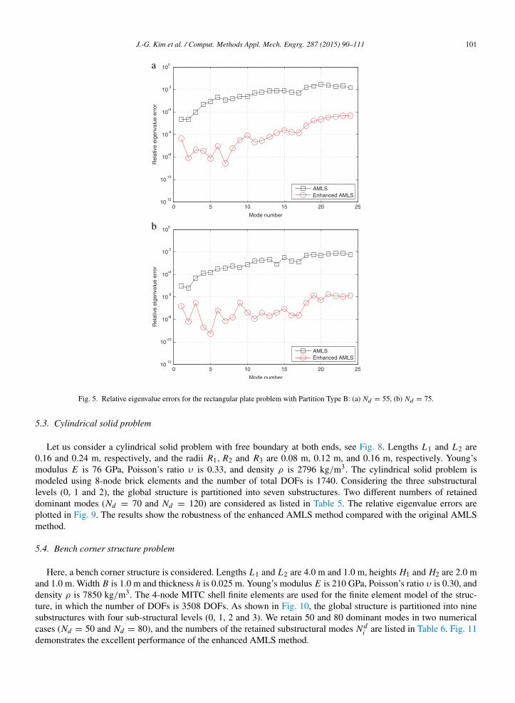
• Partition Type B: As shown in Fig. 3(b), the number of substructures is 13 and the number of substructural levelsis five (levels 0, 1, 2, 3 and 4). We retain 55 and 75 dominant modes for two numerical cases (Nd = 55 and Nd= 75).

The numbers of retained substructural modes N di in both partitioned types are listed in Tables 2 and 3 in detail. Figs. 4

and 5 present the relative eigenvalue errors obtained by the original and enhanced AMLS methods. The results showthat the enhanced AMLS method significantly outperforms the original AMLS method.

J.-G. Kim et al. / Comput. Methods Appl. Mech. Engrg. 287 (2015) 90–111 99

Table 2

Retained mode numbers N di for the rectangular plate problem with Partition Type A. All the

substructural modes are retained in the highest level substructure (level 0).

Substructural level Substructural number N di Case 1 Case 2

Level 0 7 N d7 65 65

Level 13 N d

3 3 5

6 N d6 3 5

Level 2

1 N d1 6 10

2 N d2 6 10

4 N d4 6 10

5 N d5 6 10

Total retained mode number Nd 30 50

Size of the reduced model Np 95 115

Table 3

Retained mode numbers N di for the rectangular plate problem with Partition Type B. All the

substructural modes are retained in the highest level substructure (level 0).

Substructural level Substructural number N di Case 1 Case 2

Level 0 13 N d13 65 65

Level 19 N d

9 10 13

12 N d12 4 5

Level 2

7 N d7 5 7

8 N d8 9 12

10 N d10 6 10

11 N d11 3 5

Level 33 N d

3 5 5

6 N d6 3 3

Level 4

1 N d1 4 6

2 N d2 2 3

4 N d4 3 4

5 N d5 1 2

Total retained mode number Nd 55 75

Size of the reduced model Np 120 140

5.2. Cylindrical panel problem

The performance of the proposed method is also tested in a cylindrical panel with free boundary, see Fig. 6. LengthL is 0.8 m, radius R is 0.5 m, and thickness h is 0.005 m. Young’s modulus E is 69 GPa, Poisson’s ratio ν is 0.35, anddensity ρ is 2700 kg/m3. The cylindrical panel is modeled by a 16 × 16 distorted mesh of shell finite elements andeach edge is discretized in the following ratio: L1 : L2 : L3 : . . . L16 = 16 : 15 : 14 : . . . 1 [25].

The global structure is partitioned into seven substructures with three substructural levels (levels 0, 1 and 2) asshown in Fig. 6. The numbers of retained substructural modes N d

i are listed in Table 4. The significant accuracyimprovement is observed in the enhanced AMLS method, see Fig. 7.

100 J.-G. Kim et al. / Comput. Methods Appl. Mech. Engrg. 287 (2015) 90–111

a

b

Fig. 4. Relative eigenvalue errors for the rectangular plate problem with the Partition Type A: (a) Nd = 30, (b) Nd = 50.

Table 4

Retained mode numbers N di for the cylindrical panel problem with a distorted mesh,

Partition Type A is applied. All the substructural modes are retained in the highest levelsubstructure (level 0).

Substructural level Substructural number N di Case 1 Case 2

Level 0 7 N d7 85 85

Level 13 N d

3 7 11

6 N d6 7 11

Level 2

1 N d1 4 10

2 N d2 14 29

4 N d4 14 29

5 N d5 4 10

Total retained mode number Nd 50 100

Size of the reduced model Np 135 185

J.-G. Kim et al. / Comput. Methods Appl. Mech. Engrg. 287 (2015) 90–111 101

a

b

Fig. 5. Relative eigenvalue errors for the rectangular plate problem with Partition Type B: (a) Nd = 55, (b) Nd = 75.

5.3. Cylindrical solid problem

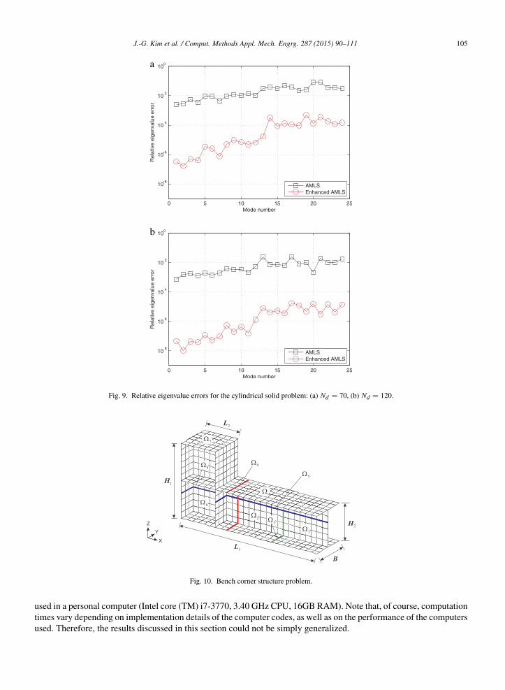
Let us consider a cylindrical solid problem with free boundary at both ends, see Fig. 8. Lengths L1 and L2 are0.16 and 0.24 m, respectively, and the radii R1, R2 and R3 are 0.08 m, 0.12 m, and 0.16 m, respectively. Young’smodulus E is 76 GPa, Poisson’s ratio υ is 0.33, and density ρ is 2796 kg/m3. The cylindrical solid problem ismodeled using 8-node brick elements and the number of total DOFs is 1740. Considering the three substructurallevels (0, 1 and 2), the global structure is partitioned into seven substructures. Two different numbers of retaineddominant modes (Nd = 70 and Nd = 120) are considered as listed in Table 5. The relative eigenvalue errors areplotted in Fig. 9. The results show the robustness of the enhanced AMLS method compared with the original AMLSmethod.

5.4. Bench corner structure problem

Here, a bench corner structure is considered. Lengths L1 and L2 are 4.0 m and 1.0 m, heights H1 and H2 are 2.0 mand 1.0 m. Width B is 1.0 m and thickness h is 0.025 m. Young’s modulus E is 210 GPa, Poisson’s ratio υ is 0.30, anddensity ρ is 7850 kg/m3. The 4-node MITC shell finite elements are used for the finite element model of the struc-ture, in which the number of DOFs is 3508 DOFs. As shown in Fig. 10, the global structure is partitioned into ninesubstructures with four sub-structural levels (0, 1, 2 and 3). We retain 50 and 80 dominant modes in two numericalcases (Nd = 50 and Nd = 80), and the numbers of the retained substructural modes N d

i are listed in Table 6. Fig. 11demonstrates the excellent performance of the enhanced AMLS method.

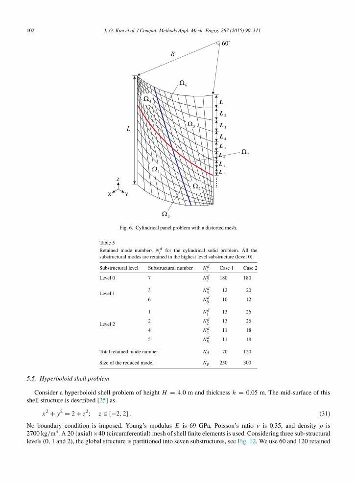
102 J.-G. Kim et al. / Comput. Methods Appl. Mech. Engrg. 287 (2015) 90–111

Fig. 6. Cylindrical panel problem with a distorted mesh.

Table 5

Retained mode numbers N di for the cylindrical solid problem. All the

substructural modes are retained in the highest level substructure (level 0).

Substructural level Substructural number N di Case 1 Case 2

Level 0 7 N d7 180 180

Level 13 N d

3 12 20

6 N d6 10 12

Level 2

1 N d1 13 26

2 N d2 13 26

4 N d4 11 18

5 N d5 11 18

Total retained mode number Nd 70 120

Size of the reduced model Np 250 300

5.5. Hyperboloid shell problem

Consider a hyperboloid shell problem of height H = 4.0 m and thickness h = 0.05 m. The mid-surface of thisshell structure is described [25] as

x2+ y2

= 2 + z2; z ∈ [−2, 2] . (31)

No boundary condition is imposed. Young’s modulus E is 69 GPa, Poisson’s ratio ν is 0.35, and density ρ is2700 kg/m3. A 20 (axial)×40 (circumferential) mesh of shell finite elements is used. Considering three sub-structurallevels (0, 1 and 2), the global structure is partitioned into seven substructures, see Fig. 12. We use 60 and 120 retained

J.-G. Kim et al. / Comput. Methods Appl. Mech. Engrg. 287 (2015) 90–111 103

a

b

Fig. 7. Relative eigenvalue errors for the cylindrical panel problem with a distorted mesh: (a) Nd = 50, (b) Nd = 100.

Table 6

Retained mode numbers N di for the bench corner structure problem. All the

substructural modes are retained in the highest level substructure (level 0).

Substructural level Substructural number N di Case 1 Case 2

Level 0 9 N d9 97 97

Level 15 N d

5 7 11

8 N d8 8 10

Level 2

3 N d3 5 6

4 N d4 11 14

6 N d6 2 7

7 N d7 11 18

Level 31 N d

1 4 9

2 N d2 2 5

Total retained mode number Nd 50 80

Size of the reduced model Np 147 177

dominant modes in two numerical cases (Nd = 60, Nd = 120), and the numbers of the retained sub-structural modesN d

i are listed in Table 7. Fig. 13 consistently demonstrates the excellent performance of the enhanced AMLS method.

104 J.-G. Kim et al. / Comput. Methods Appl. Mech. Engrg. 287 (2015) 90–111

Fig. 8. Cylindrical solid problem.

Table 7

Retained mode numbers N di for the hyperboloid shell problem. All the

substructural modes are retained in the highest level substructure (level 0).

Substructural level Substructural number N di Case 1 Case 2

Level 0 7 N d7 200 200

Level 13 N d

3 8 14

6 N d6 8 14

Level 2

1 N d1 11 23

2 N d2 11 23

4 N d4 11 23

5 N d5 11 23

Total retained mode number Nd 60 120

Size of the reduced model Np 260 320

6. Computational cost

In order to investigate the computational cost required for the enhanced AMLS method, computation times aremeasured, and compared with those of the original AMLS method. A sparse matrix computation with MATLAB is

J.-G. Kim et al. / Comput. Methods Appl. Mech. Engrg. 287 (2015) 90–111 105

a

b

Fig. 9. Relative eigenvalue errors for the cylindrical solid problem: (a) Nd = 70, (b) Nd = 120.

Fig. 10. Bench corner structure problem.

used in a personal computer (Intel core (TM) i7-3770, 3.40 GHz CPU, 16GB RAM). Note that, of course, computationtimes vary depending on implementation details of the computer codes, as well as on the performance of the computersused. Therefore, the results discussed in this section could not be simply generalized.

106 J.-G. Kim et al. / Comput. Methods Appl. Mech. Engrg. 287 (2015) 90–111

Fig. 11. Relative eigenvalue errors for the bench corner structure problem: (a) Nd = 50, (b) Nd = 80.

Table 8Computation times for calculating the lowest eigenvalues by the original and enhanced AMLS methods.

DOFs Computation time (s)Ng Np Original AMLS Enhanced AMLS

Rectangular plate (Freq. cut-off, Nd = 30) 1365 135 1.018E−01 1.182E−01Cylindrical solid (Freq. cut-off, Nd = 70) 1740 250 2.912E−01 3.001E−01Bench corner structure (Freq. cut-off, Nd = 50) 3508 147 2.216E−01 2.458E−01Hyperboloid shell (Freq. cut-off, Nd = 60) 4200 260 5.045E−01 5.248E−01

6.1. Reduced models with same size

When the size of the reduced model is the same, additional computation is required for the enhanced AMLSmethod, compared with the original AMLS method. Table 8 presents the computation times for calculating the lowesteigenvalues (mode number = 1) in the four numerical examples considered in Section 5. Note that the original andenhanced reduced transformation matrices in Eqs. (11) and (29) are used in the original and enhanced AMLS meth-ods, respectively. The results show that the additional computational cost for the enhanced AMLS method is not highcompared with the original AMLS method.

We investigate the additional computation times required for the enhanced AMLS method by increasing the numberof DOFs in the rectangular plate problem with Partition Type A in Fig. 3(a). We here consider six different meshes:20 × 12 (Ng = 1365, Np = 95), 30 × 18 (Ng = 2945, Np = 125), 40 × 24 (Ng = 5125, Np = 155), 48 × 30

J.-G. Kim et al. / Comput. Methods Appl. Mech. Engrg. 287 (2015) 90–111 107

Fig. 12. Hyperboloid shell problem.

(Ng = 7595, Np = 185), 54 × 32 (Ng = 9075, Np = 195), and 60 × 36 (Ng = 11285, Np = 215), see Fig. 14 for30 × 18 and 40 × 24 meshes.

To construct the reduced models, the number of retained dominant substructural modes is fixed as 30 in everynumerical case. Note that, as the number of DOFs increases, the size of reduced models also increases due to the DOFincrement in the highest level substructure. The computation times required for calculating the lowest eigenvalues bythe original and enhanced AMLS methods are presented in Fig. 15. This result also shows the good computationalefficiency of the enhanced AMLS method.

6.2. Reduced models with similar accuracy

For a fair comparison, the computation times of the original and enhanced AMLS methods are measured for thereduced models with similar accuracy. A turbine blade problem in Fig. 16 is considered. Length L is 35 m, thickness is0.05 m, Young’s modulus E is 210 GPa, Poisson’s ratio ν is 0.3, and density ρ is 7800 kg/m3. The detailed geometryis described in Ref. [27]. We use 10300 shell finite elements and 10100 nodes (51308 DOFs). Considering threesub-structural levels (0, 1 and 2), the global structure is partitioned into 19 substructures.

The following numerical cases are considered:

• The original AMLS method is used with the reduced model size of Np = 1260 (Nd = 60) and Np = 3100 (Nd =

1900).• The enhanced AMLS method is used with the reduced model size of Np = 1260 (Nd = 60).

Fig. 17 shows that the accuracy is similar for the reduced models using the original AMLS method with Np =

3100 (Nd = 1900) and using the enhanced AMLS method with Np = 1260 (Nd = 60). Table 9 lists the breakdownof computation time. It is observed that, with similar accuracy, the computation time required for the enhanced AMLSmethod is less than for the original AMLS method.

108 J.-G. Kim et al. / Comput. Methods Appl. Mech. Engrg. 287 (2015) 90–111

Fig. 13. Relative eigenvalue errors for the hyperboloid shell problem: (a) Nd = 60, (b) Nd = 120.

Table 9Computation times for calculating the lowest eigenvalues in the turbine blade problem. The computation times are normalized bythe total computation time required for the original AMLS method when Nd = 60.

Items Relatedequations

Normalized computation times

Original AMLS(Nd = 60)

Original AMLS(Nd = 1900)

Enhanced AMLS(Nd = 60)

Transformation procedures 11 and 270.0736 0.6272 0.0736

Solution of the substructuraleigenvalue problems

8

Calculation of the multi-levelconstraint mode matrix 9

13 0.9252 0.9252 0.9252

Solution of the reducedeigenvalue problem

3 0.0012 0.0599 0.0012

Calculation of the residualflexibility matrix Frs

a24 – – 0.0062

Inverse matrix of the reducedmass matrix Mp

a26 – – 0.0118

Total 1.0000 1.6123 1.0180

a Items only required for the enhanced AMLS method.

J.-G. Kim et al. / Comput. Methods Appl. Mech. Engrg. 287 (2015) 90–111 109

a

b

Fig. 14. Two different meshes for the rectangular plate problem with Partition Type A in Fig. 3(a): (a) 30 × 18 mesh, (b) 40 × 24 mesh.

Fig. 15. Computation times depending on the number of DOFs in the rectangular plate problem with Partition Type A in Fig. 3(a).

At this point, it is very important to note that, in this study, we tested the computational cost of the enhanced AMLSmethod for several FE models with up to 51308 DOFs using our own MATLAB implementation. Therefore, additionaltests are required considering various FE models with more than millions of DOFs. Note also that the computationalefficiency is crucial to use the enhanced AMLS method as a solver of eigenvalue problems with large DOFs. In orderto do that, much more effective computer codes and high performance computers are necessary.

110 J.-G. Kim et al. / Comput. Methods Appl. Mech. Engrg. 287 (2015) 90–111

Fig. 16. Turbine blade problem.

Fig. 17. Relative eigenvalue errors for the turbine blade problem.

7. Conclusions

In this paper, we presented a new component mode synthesis (CMS) method developed by improving the auto-mated multi-level substructuring (AMLS) method. Unlike for the original AMLS method, the residual mode effectis considered in constructing the transformation matrix. As a result, the original AMLS transformation matrix is en-hanced by the residual flexibility, in which the unknown eigenvalue is approximated using O’Callahan’s approachfrom the improved reduced system (IRS) method.

The enhanced AMLS method was then developed using this enhanced transformation matrix. As a result, global(original) structural models can be more precisely reduced, and the accuracy of reduced models is dramatically im-proved. The accuracy improvement of the enhanced AMLS method was demonstrated through numerical examples,and its computational cost was also investigated. However, as mentioned, additional numerical tests on the computa-tional cost of the enhanced AMLS method are necessary considering much larger FE models than those considered inthis study.

In order to effectively use the enhanced AMLS method as a solver of eigenvalue problems, it is important to in-crease its computational efficiency. An optimized algorithm for computer programming would be valuable, and thenefficient mode selection and error estimation techniques are essential [28–30]. In addition, the proposed method canbe used to reduce the size of system matrices in flexible multi-body systems [31–33].

J.-G. Kim et al. / Comput. Methods Appl. Mech. Engrg. 287 (2015) 90–111 111

Acknowledgments

This work was supported by the Basic Science Research Program through the National Research Foundation ofKorea (NRF) funded by the Ministry of Education, Science and Technology (No. 2014R1A1A1A05007219), and theHuman Resources Development (No. 20134030200300) of the Korea Institute of Energy Technology Evaluation andPlanning (KETEP) grant funded by the Korea government Ministry of Trade, Industry and Energy.

References

[1] R. Guyan, Reduction of stiffness and mass matrices, AIAA J. 3 (2) (1965) 380.[2] B.M. Irons, Structural eigenvalue problems: elimination of unwanted variables, AIAA J. 3 (1965) 961.[3] M.I. Friswell, S.D. Garvey, J.E.T. Penny, Model reduction using dynamic and iterated IRS techniques, J. Sound Vib. 186 (2) (1995) 311–323.[4] Y. Xia, R. Lin, A new iterative order reduction (IOR) method for eigensolutions of large structures, Internat. J. Numer. Methods Engrg. 59

(2004) 153–172.[5] W. Hurty, Dynamic analysis of structural systems using component modes, AIAA J. 3 (4) (1965) 678–685.[6] R.R. Craig, M.C.C. Bampton, Coupling of substructures for dynamic analysis, AIAA J. 6 (7) (1965) 1313–1319.[7] R.H. MacNeal, Hybrid method of component mode synthesis, Comput. Struct. 1 (4) (1971) 581–601.[8] W.A. Benfield, R.F. Hruda, Vibration analysis of structures by component mode substitution, AIAA J. 9 (1971) 1255–1261.[9] S. Rubin, Improved component-mode representation for structural dynamic analysis, AIAA J. 13 (8) (1975) 995–1006.

[10] K.C. Park, Y.H. Park, Partitioned component mode synthesis via a flexibility approach, AIAA J. 42 (6) (2004) 1236–1245.[11] D.J. Rixen, A dual Craig–Bampton method for dynamic substructuring, J. Comput. Appl. Math. 168 (1–2) (2004) 383–391.[12] K.C. Park, J.G. Kim, P.S. Lee, A mode selection criterion based on flexibility approach in component mode synthesis, in: Proceeding 53th

AIAA/ASME/ASCE/AHS/ASC Structures, Structural Dynamics, and Materials Conference Hawaii, USA, 2012.[13] F. Bourquin, Analysis and comparison of several component mode synthesis methods on one dimensional domains, Numer. Math. 58 (1)

(1990) 11–33.[14] F. Bourquin, Component mode synthesis and eigenvalues of second order operators: discretization and algorithm, Math. Model. Numer. Anal.

26 (3) (1992) 385–423.[15] F. Bourquin, F. d’Hennezel, Intrinsic component mode synthesis and plate vibrations, Comput. Struct. 44 (1–2) (1992) 315–324.[16] F. Bourquin, F. d’Hennezel, Numerical study of an intrinsic component mode synthesis method, Comput. Methods Appl. Mech. Engrg. 97 (1)

(1992) 49–76.[17] J.K. Bennighof, R.B. Lehoucq, An automated multi-level substructuring method for eigenspace computation in linear elastodynamics, SIAM

J. Sci. Comput. 25 (6) (2004) 2084–2106.[18] J. O’Callahan, A procedure for an improved reduced system (IRS) model, in: Proceeding of the 7th International Modal Analysis Conference,

CT, Bethel, 1989.[19] M.F. Kaplan, Implementation of automated multi-level substructuring for frequency response analysis of structures (Ph.D. thesis), Department

of Aerospace Engineering & Engineering Mechanics, University of Texas at Austin, Austin, TX, 2001.[20] J.K. Bennighof, M.F. Kaplan, Frequency sweep analysis using multi-level substructuring, global modes and iteration, in: Proceedings of the

39th Annual AIAA Structural Dynamics and Materials Conference, Long Beach, CA, 1998.[21] S.H. Boo, J.G. Kim, P.S. Lee, Error estimation for the automated multi-level substructuring method, Internat. J. Numer. Methods Engrg.

(2015) submitted for publication.[22] A. Ibrahimbegovic, H.C. Chen, E.L. Wilson, R.L. Taylor, Ritz method for dynamic analysis of linear systems with non-proportional damping,

Int. J. Earthq. Eng. Struct. Dyn. 19 (1990) 877–889.[23] E.N. Dvorkin, K.J. Bathe, A continuum mechanics based four-node shell element for general nonlinear analysis, Eng. Comput. 1 (1) (1984)

77–88.[24] K.J. Bathe, E.N. Dvorkin, A formulation of general shell elements-the use of mixed interpolation of tensorial components, Internat. J. Numer.

Methods Engrg. 22 (3) (1986) 697–722.[25] Y. Lee, K.H. Yoon, P.S. Lee, Improving the MITC3 shell finite element by using the Hellinger–Reissner principle, Comput. Struct. 110–111

(2012) 93–106.[26] Y. Lee, P.S. Lee, K.J. Bathe, The MITC3+ shell finite element and its performance, Comput. Struct. 138 (2014) 12–23.[27] K.H. Yoon, Y. Lee, P.S. Lee, A continuum mechanics based 3-D beam finite element with warping displacements and its modeling capabilities,

Struct. Eng. Mech. 43 (4) (2012) 411–437.[28] J.G. Kim, K.H. Lee, P.S. Lee, Estimating relative eigenvalue errors in the Craig–Bampton method, Comput. Struct. 139 (2014) 54–64.[29] J.G. Kim, P.S. Lee, An accurate error estimator for Guyan reduction, Comput. Methods Appl. Mech. Engrg. 278 (2014) 1–19.[30] A. Ibrahimbegovic, E.L. Wilson, Automated truncation of Ritz vector basis in modal transformation, ASCE J. Engrg. Mech. Div. 116 (1990)

2506–2520.[31] O.P. Agrawal, A.A. Shabana, Dynamic analysis of multibody systems using component modes, Comput. Struct. 21 (6) (1985) 1301–1312.[32] J. Gerstmayr, J.A.C. Ambrosio, Component mode synthesis with constant mass and stiffness matrices applied to flexible multibody systems,

Internat. J. Numer. Methods Engrg. 73 (2008) 1518–1546.[33] A. Ibrahimbegovic, R.L. Taylor, H. Lim, Nonlinear dynamics of flexible multibody systems, Comput. Struct. 81 (2003) 1113–1132.