An energy-based limit state function for estimation of ...

Shock and Vibration 20 (2013) 933–950 933DOI 10.3233/SAV-130795IOS Press

An energy-based limit state function forestimation of structural reliability in shockenvironments

Michael A. GuthrieAnalytical Structural Dynamics, Org. 1523, Sandia National Laboratories, MS 0346, P.O. Box 5800, Albuquerque,NM 87185, USATel.: +1 505 284 1357; E-mail: [email protected]

Received 6 September 2012

Revised 17 December 2012

Accepted 13 April 2013

Abstract. A limit state function is developed for the estimation of structural reliability in shock environments. This limit statefunction uses peak modal strain energies to characterize environmental severity and modal strain energies at failure to characterizethe structural capacity. The Hasofer-Lind reliability index is briefly reviewed and its computation for the energy-based limit statefunction is discussed. Applications to two degree of freedom mass-spring systems and to a simple finite element model areconsidered. For these examples, computation of the reliability index requires little effort beyond a modal analysis, but stillaccounts for relevant uncertainties in both the structure and environment. For both examples, the reliability index is observed toagree well with the results of Monte Carlo analysis. In situations where fast, qualitative comparison of several candidate designsis required, the reliability index based on the proposed limit state function provides an attractive metric which can be used tocompare and control reliability.

Keywords: Shock, structural reliability, limit state function

1. Introduction

A great deal of literature, beginning with the work of Hudson [1] and Housner [2,3], has focused on the use ofenergy to characterize earthquake excitation of structures. These energy metrics have become widely accepted in theearthquake engineering community, but until recently have received little attention elsewhere. However, recent workin the structural dynamics field has focused on using energy to characterize the severity of shock and vibration envi-ronments [4–6]. These energy-based metrics offer a number of advantages over the more traditional shock responsespectrum, such as greater meaning for multiple degree of freedom systems, closer correspondence to material failurecriteria, and greater ability to distinguish between waveforms with different temporal characteristics and durations.Perhaps the greatest benefit is that energy-based characterization of shock and vibration environments allows for thecomparison of component test environments with requirements through scalar estimates of margin, which can thenbe used in reliability analysis.

A natural extension of the energy-based characterization of shock and vibration environments is the prediction ofcomponent reliability in these environments using energy-based severity metrics. In this context, component margintesting is replaced by finite element modeling in order to establish the energy capacity of the structure. The energycapacity can then be compared probabilistically with the energy demands imposed by the environment to obtainestimates of component reliability using methods from the structural reliability literature (e.g., [7,8]).

ISSN 1070-9622/13/$27.50 c© 2013 – IOS Press and the authors. All rights reserved

934 M.A. Guthrie / An energy-based limit state function for estimation of structural reliability in shock environments

An important concept from the structural reliability literature is that of the limit state function. Limit state func-tions are scalar functions g(Z) such that failure occurs if and only if g(Z) < 0, where the variables Z are called thebasic variables. The hypersurface defined by g(Z) = 0 is known as the limit state surface and it partitions the spaceof basic variables into a safe set for which g(Z) > 0 and a failure set for which g(Z) < 0. Limit state functionsare used throughout the structural reliability literature to define failure in terms of applied forces, yield stresses,dimensions, etc.

Structural reliability methods are often classified by the amount of statistical information about the basic variableswhich they require [7]. In level II methods, it is assumed that estimates of the expected value and covariance ofthe basic variables are available. The advantage of these methods is that they eliminate the need for determiningprobability distributions for each basic variable. The cost of this simplification is that level II methods cannot predictreliability directly; instead they provide reliability indices which can be used to compare and control reliability.For example, these methods could be very useful during the design process when one wishes to determine whichof several designs is more reliable in a given environment or to assess the influence of a design change on thereliability. However, the reliability index does not have a direct interpretation in terms of the probability of failurewithout assuming probability distributions for the basic variables – its value is as a predictor of reliability for onestructure relative to another. Perhaps the most common level II method is the use of the Hasofer-Lind reliabilityindex [9], which is defined as the shortest distance between the mean point and the limit state surface in the spaceof standardized, decorrelated basic variables. In contrast to level II methods, level III methods predict reliability butrequire probability density functions for each of the basic variables.

In this paper, a limit state function based upon the peak modal strain energies and modal strain energies at failureis developed for the estimation of structural reliability in shock environments. Due to the difficulty of approximat-ing the probability distributions for these basic variables, level II reliability methods are considered exclusively. TheHasofer-Lind reliability index can be calculated based upon the proposed limit state function and provides a measureof the structure’s reliability. This approach could be very valuable during the design process, when fast, qualitativecomparison of the relative reliabilities of various design options is required. In such situations, Monte Carlo analysisis often too computationally intensive to provide the fast turnaround required to support design studies. The reliabil-ity approach developed here requires little effort beyond a modal analysis, but still accounts for relevant uncertaintiesin both the structure and environment. A second advantage of this approach is that it provides important informationabout the sensitivity of the structure’s reliability to the frequency content of the input.

This document begins with the mathematical development of the limit state function, followed by a brief descrip-tion of the Hasofer-Lind reliability index and its computation for the proposed limit state function. The reliabilityapproach is then applied to two degree of freedom (DOF) base excited mass-spring systems as well as a simple finiteelement model. In both cases, the reliability indices are compared with the results of Monte Carlo analysis and it isseen that the two approaches produce similar results and that the reliability approach is much faster and easier toimplement.

2. Development of limit state function

Consider a general linear structure with mass-normalized mode shapes φi and natural frequencies ωi which canbe accurately represented in terms of a subset of n of these modes. Suppose that the structure is subjected to ashock input through its base which is characterized in terms of peak modal strain energies Ei and that failure of thestructure is defined through m inequalities of the form:

|fj(d)| > ffail,j for any j = 1 . . .m (1)

where fj(d) can denote any linear function of displacement used to define failure of the structure (e.g., force, stress,etc.) and ffail,j � 0 denotes the value of that quantity at which failure occurs. Both the shock input and the structureare treated probabilistically and a measure of the reliability is desired. For this problem, a limit state function can bedeveloped for each of the m constraints. Begin by noting that for a general shape Φα where α is an arbitrary vectorof modal coordinates and Φ denotes the mass-normalized modal matrix, the strain energy in mode i is:

εi =1

2ω2i α

2i for i = 1 . . . n (2)

M.A. Guthrie / An energy-based limit state function for estimation of structural reliability in shock environments 935

Next, consider scaling the shape Φα by a constant c such that fj(d) = ffail,j . Since fj(d) is linear,

c =ffail,j

fj (Φα)(3)

The strain energy in mode i when the structure is scaled such that fj(d) = ffail,j is therefore:

εi =1

2ω2i α

2i

f2fail,j

fj (Φα)2 for i = 1 . . . n, j = 1 . . .m (4)

By rewriting the modal coordinates as

α =

⎡⎢⎣α1

...αn

⎤⎥⎦ = αn

⎡⎢⎢⎢⎣

α1/αn

...αn−1/αn

1

⎤⎥⎥⎥⎦ def

= αn

⎡⎢⎢⎢⎣

ξ1...

ξn−1

1

⎤⎥⎥⎥⎦ def

= αnξ (5)

Equation (2) can be rewritten as

εi =1

2ω2i ξ

2i

f2fail,j

fj (Φξ)2 for i = 1 . . . n− 1, j = 1 . . .m (6)

εn =1

2ω2n

f2fail,j

fj (Φξ)2 for j = 1 . . .m (7)

For each value of j, these equations define an n − 1 dimensional strain energy at failure surface parameterized byξ1 . . . ξn−1. A more useful definition of these surfaces than the parametric one given in Eqs (6) and (7) would relatethe modal strain energies εi to one another. Therefore the following mathematical form is proposed to describe thestrain energy at failure surfaces:

εn = εfail,n|j

⎛⎝1 +

n−1∑i=1

si

√εi

εfail,i|j

⎞⎠

2

for j = 1 . . .m (8)

where si = ±1 ∀ i and the strain energy at failure of element j for pure deformation in mode i is

εfail,i|jdef=

1

2ω2i

f2fail,j

fj (φi)2 (9)

In order to verify that Eq. (8) represents the surfaces defined parametrically in Eqs (6) and (7), substitute Eqs (6),(7), and (9) into Eq. (8) and simplify to obtain:

fj (φn)2 =

(|fj (Φξ)|+

n−1∑i=1

si |ξi| |fj (φi)|)2

(10)

Since the functions fj(x) are linear, this can be rewritten as

fj (φn)2 =

(∣∣∣∣∣n∑

i=1

ξifj (φi)

∣∣∣∣∣+n−1∑i=1

si |ξi| |fj (φi)|)2

=

(sgn

(n∑

i=1

ξifj (φi)

)n∑

i=1

ξifj (φi) +

n−1∑i=1

sgn (ξi) sgn (fj (φi)) siξifj (φi)

) (11)


By choosing

si = −sgn (ξi) sgn

(n∑

k=1

ξkfj (φk)

)sgn (fj (φi)) (12)

the equation above becomes

fj (φn)2 =

(sgn

(n∑

i=1

ξifj (φi)

)(n∑

i=1

ξifj (φi)−n−1∑i=1

ξifj (φi)

))2

(13)

which is clearly true. Thus the functional form defined in Eq. (8) is valid as long as the functions fj(x) are linear.Equation (8) defines 2n−1 strain energy at failure surfaces associated with each of the permutations of the si foreach of the m constraints, but if ε1 . . . εn−1 are small enough that

n−1∑i=1

√εi

εfail,i|j< 1 (14)

then the surface with si = −1 ∀ i is the most conservative in the sense that the value of εn required for failure isless for si = −1 ∀ i than for any other permutation of the si. If the condition in Eq. (14) does not hold, failure of thestructure is possible since one or more of the limit state surfaces as defined by Eq. (8) has been exceeded. Thereforeit is assumed that failure occurs whenever Eq. (14) does not hold, and that failure occurs on the branch of the strainenergy at failure surface with si = −1 ∀ i when the condition in Eq. (14) does hold. These assumptions lead to thefollowing limit state function for each constraint in the 2n basic variables Ei and εfail,i|j :

gj

(Ei, εfail,i|j

)=

⎧⎪⎪⎪⎪⎪⎨⎪⎪⎪⎪⎪⎩

εfail,n|j(1−

n−1∑i=1

√Ei

εfail,i|j

)2

− En ifn−1∑i=1

√Ei

εfail,i|j< 1

εfail,n|j(1−

n−1∑i=1

√Ei

εfail,i|j

)− En otherwise

(15)

Note that the second part of this definition is arbitrary: any limit state function which is strictly negative whenthe condition in Eq. (14) does not hold would be valid since it is assumed that the structure fails in this case.The definition in Eq. (15) has been adopted for computational convenience. It should be noted that the approachdeveloped here is limited to structures for which failure can be defined in terms of mechanical criteria of the typespecified in Eq. (1). Since it depends upon the FEM to establish the strain energy at failure in each of the structure’smodes, the approach is unable to predict failures which cannot be modeled using the underlying FEM (e.g., electricalfailures). While the derivation above is only valid for failure criteria which depend linearly on displacement, thefinal example problem considered in this paper suggests that the limit state function can be applied when the failurecriterion does not depend linearly on displacement without great loss of accuracy. The extension of the limit statefunction to these cases will be considered more rigorously in future work.

Two important conservative assumptions have been made in developing the limit state function of Eq. (15) fromEq. (8). First, each of the modal strain energies has been assumed to equal its peak value. In reality, the modalstrain energies εi are functions of time which each peak at distinct times, but by setting these energies equal totheir peak values Ei, it is assumed that they all peak simultaneously. The second conservative assumption made indeveloping Eq. (15) is in using the most conservative branch of the strain energy at failure surface from Eq. (8). Thus,if gj > 0 ∀ j, failure as defined by Eq. (1) is impossible, but if gj < 0 for one or more values of j the system doesnot necessarily fail since it might fail on one of the less conservative branches of Eq. (8). The physical meaning ofthese branches is explored in an example problem later in this paper. It is anticipated that the assumptions underlyingthe limit state function will introduce considerable conservative bias to estimates of the probability of failure if thelimit state function is used for level III reliability analysis. However, it is also anticipated that these assumptionswill be consistently conservative from structure to structure so that, when the limit state function is used for levelII reliability analysis, the reliability indices will accurately reflect the reliability of one structure relative to another.The reliability indices will thus still be useful for their intended purpose: to compare and control the reliability ofstructures.


3. Hasofer-Lind reliability index

One of the most widely used level II reliability methods is the Hasofer-Lind reliability index [9]. This index repre-sents the minimum distance between the origin and the limit state surface in the space of standardized, decorrelatedbasic variables. For a wide variety of distributions, the probability content of the basic variables will decline expo-nentially with distance from the origin, so the probability of failure will often be dominated by the small region ofthe failure domain nearest the origin. In these cases, the distance of this region from the origin, or the Hasofer-Lindreliability index, provides a good measure of reliability. For a problem with only a single basic variable, this index isequal to the distance from the mean point to the failure point measured in standard deviations of the basic variable,which corresponds to the Cornell reliability index [10]. The mathematics of the Hasofer-Lind reliability index arebriefly reviewed below and applied to the limit state function defined in Eq. (15).

Denote the vector of basic variables by Z . For the problem considered in this paper,

Z =[E1 E2 . . . En εfail,1|j εfail,2|j . . . εfail,n|j

](16)

The limit state function defined in Eq. (15) can be rewritten in terms of the basic variables as

gj(Z) =

⎧⎪⎪⎪⎪⎨⎪⎪⎪⎪⎩Z2n

(1−

n−1∑i=1

√Zi

Zi+n

)2

− Zn ifn−1∑i=1

√Zi

Zi+n< 1

Z2n

(1−

n−1∑i=1

√Zi

Zi+n

)− Zn otherwise

(17)

In general, the basic variables are correlated and have non-zero means and non-unit variances. Therefore the co-variance matrix CZ will be non-diagonal and the expected value E [Z] �= 0. Define the standardized, decorrelatedvariables X as follows:

X = A (Z −E [Z]) (18)

where the matrix A is chosen such that X has covariance equal to the identity matrix:

CX = ACZAT = I (19)

The matrix A satisfying Eq. (19) has rows which are the transposed eigenvectors of CZ , vTi , divided by the squareroot of the corresponding eigenvalue, ri:

A =

⎡⎢⎣

vT1 /√r1

...vT2n/

√r2n

⎤⎥⎦ (20)

The variables X defined in this way are uncorrelated and have zero mean and unit variance. The Hasofer-Lindreliability index is defined as the minimum distance from the origin to the limit state surface in X-space:

βj = mingj(x)=0

√xTx (21)

where x denotes a realization of the standardized variables X . Equation (21) can be restated in terms of realizationsof the basic variables Z using Eqs (18) and (19):

βj = mingj(z)=0

√(z −E [Z])

TC−1

Z (z −E [Z]) (22)


The point z∗ satisfying Eq. (22) is known as the most probable point (MPP), since it is the point in the failure domainwith the greatest probability content. In [9], Hasofer and Lind proposed a simple iterative scheme for finding theMPP:

z(k+1) = E [Z] + CZ∇gj

(z(k)) (z(k) −E [Z]

)T ∇gj(z(k))− gj

(z(k))

∇gj(z(k))T

CZ∇gj(z(k)) (23)

where the initial point is taken to be the mean (z(0) = E [Z]) and the gradient of the limit state function is

(∇gj)i (Z) =

⎧⎪⎪⎪⎨⎪⎪⎪⎩−Z2n

(1−

n−1∑k=1

√Zk

Zk+n

)1√

ZiZi+n

ifn−1∑k=1

√Zk

Zk+n< 1

−1

2Z2n

1√ZiZi+n

otherwise

for i = 1 . . . n− 1 (24)

(∇gj)n (Z) = −1

(∇gj)i (Z) =

⎧⎪⎪⎪⎪⎪⎨⎪⎪⎪⎪⎪⎩

Z2n

(1−

n−1∑k=1

√Zk

Zk+n

)√Zi−n

Z3i

ifn−1∑k=1

√Zk

Zk+n< 1

1

2Z2n

√Zi−n

Z3i

otherwise

for i = n+ 1 . . . 2n− 1

(∇gj)2n (Z) =

⎧⎪⎪⎪⎪⎨⎪⎪⎪⎪⎩

(1−

n−1∑k=1

√Zk

Zk+n

)2

ifn−1∑k=1

√Zk

Zk+n< 1

(1−

n−1∑k=1

√Zk

Zk+n

)otherwise

Since Eq. (15) defines m limit state functions, Eq. (23) must be applied with each of these to find m independentreliability indices β1, β2, . . . βm. The system reliability index is then equal to the minimum of these:

β = minj=1...m βj (25)

The vector x∗ satisfying Eq. (21) is related to the sensitivity of the reliability index to the decorrelated, standardizedvariables xi:

x∗i = β

∂β

∂xi(26)

The change in the reliability index for a change in the expected value of each of the original basic variables Zi byone standard deviation can be found by combining Eqs (18) and (26):

∂β

∂ (E [Zi] /σi)= −σi

β

2n∑j=1

Ajix∗j (27)

In order to determine the Hasofer-Lind reliability index, estimates of the means, variances, and correlation coeffi-cients for the peak modal strain energies and modal strain energies at failure are required. It is assumed here thatthe mean and variance for each of these variables is available and that the peak modal strain energies are uncor-related with the modal strain energies at failure. Since the peak modal strain energies are largely functions of theenvironment and the modal strain energies at failure are functions of the structural properties, it is expected that thiswill typically be an accurate assumption. The correlation between the peak modal strain energies is a function ofthe environment, and an analysis of this correlation for general environments is beyond the scope of this paper. For


Fig. 1. Base-excited, two DOF systems (from left to right, structures 1–4).

well-separated natural frequencies and environments with broad frequency content, it is expected that this correla-tion will often be small, so the peak modal strain energies are assumed to be uncorrelated with one another in theexample problems of Sections 4 and 5. Furthermore, the modal strain energies at failure are assumed to be perfectlycorrelated with one another in these problems. This assumption holds exactly for cases in which the natural modesand frequencies are deterministic and only the failure criteria are uncertain, and it is expected that it will remain anaccurate assumption for cases in which the variability in the natural modes and frequencies is small compared tothe variability in the failure criteria. Nonetheless, the approach is general and can account for arbitrary correlationsamongst the basic variables when these correlations are known.

4. Application to mass-spring systems

To illustrate the use of the energy-based limit state function in a level II reliability analysis, the four base-excited,two DOF systems shown in Fig. 1 are considered. While it is not clear a priori which of these systems is most reliablein a given shock environment, this section will demonstrate that the Hasofer-Lind reliability index calculated usingthe energy-based limit state function provides an excellent metric of each system’s reliability. Each system is dampedwith 5% modal damping and fails when the force in either of the springs exceeds the corresponding failure forceffail,1 or ffail,2. The strain energy at failure of spring j for pure deformation in mode i is given by:

εfail,i|j =1

2ω2i

f2fail,j

|Pjφi|2(28)

where P denotes the matrix that, when post-multiplied by the displacement, produces the spring forces:

P =

[k1 0−k2 k2

](29)

and Pj denotes row j of this matrix. Consider the following nominal values of the system parameters:

m = 0.01 kg, k = 400π2 N/m, ffail,1 = 10 N, and ffail,2 = 3.9 N (30)

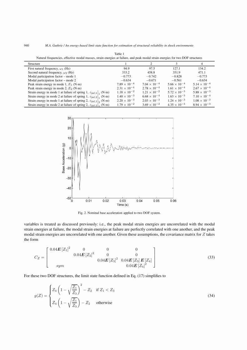
Each system is subjected to the nominal base acceleration shown in Fig. 2. The nominal natural frequencies, effectivemodal masses, strain energies at failure, and peak modal strain energies for each system are given in Table 1. Thepeak modal strain energies are calculated by integrating the modal responses to the given base acceleration usingthe central difference method and then employing the following equation:

Ei =1

2ω2i α

2i,max (31)

where αi,max denotes the maximum of the absolute value of the modal displacement in mode i.The basic variables for spring j are:

Z =[Z1 Z2 Z3 Z4

]=[E1 E2 εfail,1|j εfail,2|j

](32)

For each structure, the expected values of the basic variables are set equal to the nominal values from Table 1.In addition, each basic variable is assigned a coefficient of variation equal to 0.2. The correlation between basic


Table 1Natural frequencies, effective modal masses, strain energies at failure, and peak modal strain energies for two DOF structures

Structure 1 2 3 4First natural frequency, ω1 (Hz) 94.9 97.5 127.1 134.2Second natural frequency, ω2 (Hz) 333.2 458.8 351.9 471.1Modal participation factor – mode 1 −0.773 −0.742 −0.828 −0.773Modal participation factor – mode 2 −0.634 −0.671 −0.561 −0.634Peak strain energy in mode 1, E1 (N·m) 7.89 × 10−4 7.04 × 10−4 5.66 × 10−4 5.14 × 10−4

Peak strain energy in mode 2, E2 (N·m) 2.31 × 10−4 2.78 × 10−4 1.61 × 10−4 2.67 × 10−4

Strain energy in mode 1 at failure of spring 1, εfail,1∣∣1

(N·m) 1.18 × 10−2 1.21 × 10−2 5.72 × 10−3 5.88 × 10−3


(N·m) 1.40 × 10−3 6.68 × 10−4 1.63 × 10−3 7.10 × 10−4


(N·m) 2.20 × 10−3 2.03 × 10−3 1.24 × 10−3 1.08 × 10−3


(N·m) 1.79 × 10−2 3.69 × 10−2 4.35 × 10−3 8.94 × 10−3

Fig. 2. Nominal base acceleration applied to two DOF system.

variables is treated as discussed previously: i.e., the peak modal strain energies are uncorrelated with the modalstrain energies at failure, the modal strain energies at failure are perfectly correlated with one another, and the peakmodal strain energies are uncorrelated with one another. Given these assumptions, the covariance matrix for Z takesthe form

CZ =

⎡⎢⎢⎣

0.04E [Z1]2 0 0 0

0.04E [Z2]2 0 0

0.04E [Z3]2

0.04E [Z3]E [Z4]

sym 0.04E [Z4]2

⎤⎥⎥⎦ (33)

For these two DOF structures, the limit state function defined in Eq. (17) simplifies to

g(Z) =

⎧⎪⎪⎪⎨⎪⎪⎪⎩Z4

(1−√

Z1

Z3

)2

− Z2 if Z1 < Z3

Z4

(1−√

Z1

Z3

)− Z2 otherwise

(34)


Table 2Reliability indices, sensitivity vectors, and Monte Carlo reliabilities for two DOF structures

Structure 1 2 3 4Hasofer-lind reliability index, β 2.20 0.96 1.02 0.78Spring governing β Spring 2 Spring 1 Spring 2 Spring 1Sensitivity vector from Eq. (20) −0.395 −0.186 −0.502 −0.232

−0.079 −0.480 −0.146 −0.4660.779 0.230 0.670 0.2780.137 0.627 0.182 0.575

Overall reliability from Monte Carlo 98.85% 91.47% 93.23% 84.41%Spring 1 reliability – Monte Carlo 99.79% 92.11% 99.82% 91.96%Spring 2 reliability – Monte Carlo 99.06% 99.36% 93.41% 92.45%

which has gradient from Eq. (24):

∇g =

⎡⎢⎢⎢⎢⎢⎢⎢⎢⎢⎢⎢⎣

−Z4

(1−√

Z1

Z3

)1√Z1Z3

−1

Z4

(1−√

Z1

Z3

)√Z1

Z33(

1−√

Z1

Z3

)2

⎤⎥⎥⎥⎥⎥⎥⎥⎥⎥⎥⎥⎦

if Z1 < Z3 and ∇g =

⎡⎢⎢⎢⎢⎢⎢⎢⎢⎢⎢⎣

−1

2Z4

1√Z1Z3

−1

1

2Z4

√Z1

Z33(

1−√

Z1

Z3

)

⎤⎥⎥⎥⎥⎥⎥⎥⎥⎥⎥⎦

otherwise (35)

Given these expressions for the limit state function and its gradient as well as the expected value and covariance ofthe basic variables, the iterative procedure given in Eq. (23) can be applied to find the MPP and the Hasofer-Lindreliability index for each of the structures considered. The reliability index, the spring with the minimum reliabilityindex, and the sensitivity vector from Eq. (27) for each structure are stated in Table 2. The reliability indices suggestthat structure 1 is by far the most reliable in the given environment, followed by structures 3, 2, and 4. The resultsalso suggest that structures 1 and 3 are most likely to fail at spring 2, while structures 2 and 4 are most likely to failat spring 1, since these are the springs governing the reliability index for each structure. The sensitivity vectors listedin Table 2 provide information that could be useful in the design process. For example, the reliability of structure1 is most sensitive to the peak strain energy in mode 1 and strain energy at failure in mode 1. This suggests designchanges that could make structure 1 more reliable, such as increasing the damping in mode 1, shifting the frequencyof mode 1 so it receives less energy from the input, and increasing the failure force for spring 2. While much of thisinformation could be easily determined through other means for these simple systems, the technique presented herecan be readily applied to more complicated structures, as illustrated in Section 5.

In order to provide confidence in the results from the reliability analysis, a Monte Carlo analysis was also per-formed. Base accelerations were generated as exponentially decayed sums of sines at each of the structure’s naturalfrequencies:

Ag = e−ct2∑

i=1

Ai sinωit (36)

where the decay constant is chosen to be c = 15 1/s. The coefficients Ai are independent and normally distributedwith means and variances selected such that the base acceleration delivers peak modal strain energies which havemeans and standard deviations matching the nominal values listed in Table 1 and the assumed coefficient of variationof 0.2. That is, the means and variances of the coefficients Ai were selected to satisfy the following system ofequations:

H(y) ≡ h(y)− h∗ = 0 (37)

where y is a vector containing the means and variances of the coefficients Ai, h(y) denotes a vector of the meansand standard deviations of the peak modal strain energies for a given value of y, and h∗ represents a vector of the


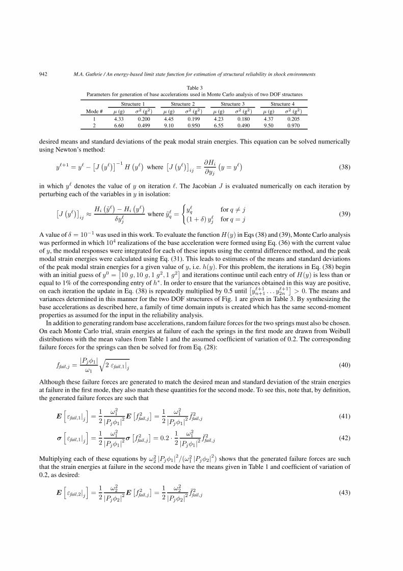
Table 3Parameters for generation of base accelerations used in Monte Carlo analysis of two DOF structures

Structure 1 Structure 2 Structure 3 Structure 4Mode # μ (g) σ2 (g2) μ (g) σ2 (g2) μ (g) σ2 (g2) μ (g) σ2 (g2)

1 4.33 0.200 4.45 0.199 4.23 0.180 4.37 0.2052 6.60 0.499 9.10 0.950 6.55 0.490 9.50 0.970

desired means and standard deviations of the peak modal strain energies. This equation can be solved numericallyusing Newton’s method:

y�+1 = y� − [J (y�)]−1H(y�)

where[J(y�)]

ij=

∂Hi

∂yj

(y = y�

)(38)

in which y� denotes the value of y on iteration �. The Jacobian J is evaluated numerically on each iteration byperturbing each of the variables in y in isolation:

[J(y�)]

ij≈ Hi

(y�)−Hi

(y�)

δy�jwhere y�q =

{y�q for q �= j

(1 + δ) y�j for q = j(39)

A value of δ = 10−1 was used in this work. To evaluate the functionH(y) in Eqs (38) and (39), Monte Carlo analysiswas performed in which 104 realizations of the base acceleration were formed using Eq. (36) with the current valueof y, the modal responses were integrated for each of these inputs using the central difference method, and the peakmodal strain energies were calculated using Eq. (31). This leads to estimates of the means and standard deviationsof the peak modal strain energies for a given value of y, i.e. h(y). For this problem, the iterations in Eq. (38) beginwith an initial guess of y0 =

[10 g, 10 g, 1 g2, 1 g2

]and iterations continue until each entry of H(y) is less than or

equal to 1% of the corresponding entry of h∗. In order to ensure that the variances obtained in this way are positive,on each iteration the update in Eq. (38) is repeatedly multiplied by 0.5 until

[y�+1n+1 . . . y

�+12n

]> 0. The means and

variances determined in this manner for the two DOF structures of Fig. 1 are given in Table 3. By synthesizing thebase accelerations as described here, a family of time domain inputs is created which has the same second-momentproperties as assumed for the input in the reliability analysis.

In addition to generating random base accelerations, random failure forces for the two springs must also be chosen.On each Monte Carlo trial, strain energies at failure of each the springs in the first mode are drawn from Weibulldistributions with the mean values from Table 1 and the assumed coefficient of variation of 0.2. The correspondingfailure forces for the springs can then be solved for from Eq. (28):

ffail,j =|Pjφ1|ω1

√2 εfail,1|j (40)

Although these failure forces are generated to match the desired mean and standard deviation of the strain energiesat failure in the first mode, they also match these quantities for the second mode. To see this, note that, by definition,the generated failure forces are such that

E[εfail,1|j

]=

1

2

ω21

|Pjφ1|2E[f2

fail,j

]=

1

2

ω21

|Pjφ1|2f2

fail,j (41)

σ[εfail,1|j

]=

1

2

ω21

|Pjφ1|2σ[f2

fail,j

]= 0.2 · 1

2

ω21

|Pjφ1|2f2

fail,j (42)

Multiplying each of these equations by ω22 |Pjφ1|2/(ω2

1 |Pjφ2|2) shows that the generated failure forces are suchthat the strain energies at failure in the second mode have the means given in Table 1 and coefficient of variation of0.2, as desired:

E[εfail,2|j

]=

1

2

ω22

|Pjφ2|2E[f2

fail,j

]=

1

2

ω22

|Pjφ2|2f2

fail,j (43)


Table 4Percentage difference between nominal values and actual values from Monte Carlo analysis for mean and standard deviation of peak modal strainenergies and strain energies at failure

Structure 1 Structure 2 Structure 3 Structure 4Mode 1 Mode 2 Mode 1 Mode 2 Mode 1 Mode 2 Mode 1 Mode 2

% Diff. in mean of peak modal strain energies 0.03% −1.88% 0.77% −1.76% 0.56% 0.15% 0.08% −1.37%% Diff. in Std. Dev. of peak modal strain energies 0.59% −0.60% 0.59% 0.17% −0.33% −1.01% 0.93% −1.97%% Diff. in mean of strain energies at failure of spring 1 0.09% 0.09% 0.02% 0.02% −0.21% −0.21% 0.09% 0.09%% Diff. in Std. Dev. of strain energies at failure of spring 1 −0.69% −0.69% 0.52% 0.52% 0.78% 0.78% 0.58% 0.58%% Diff. in mean of strain energies at failure of spring 2 −0.09% −0.09% −0.05% −0.05% −0.28% −0.28% −0.23% −0.23%% Diff. in Std. Dev. of strain energies at failure of spring 2 −0.35% −0.35% −0.20% −0.20% 0.95% 0.95% −0.78% −0.78%

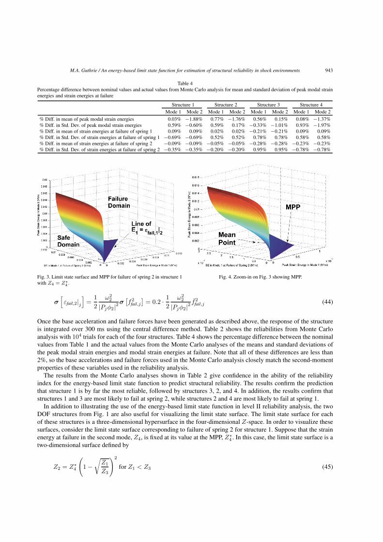
Fig. 3. Limit state surface and MPP for failure of spring 2 in structure 1with Z4 = Z∗

4 .Fig. 4. Zoom-in on Fig. 3 showing MPP.

σ[εfail,2|j

]=

1

2

ω22

|Pjφ2|2σ[f2

fail,j

]= 0.2 · 1

2

ω22

|Pjφ2|2f2

fail,j (44)

Once the base acceleration and failure forces have been generated as described above, the response of the structureis integrated over 300 ms using the central difference method. Table 2 shows the reliabilities from Monte Carloanalysis with 104 trials for each of the four structures. Table 4 shows the percentage difference between the nominalvalues from Table 1 and the actual values from the Monte Carlo analyses of the means and standard deviations ofthe peak modal strain energies and modal strain energies at failure. Note that all of these differences are less than2%, so the base accelerations and failure forces used in the Monte Carlo analysis closely match the second-momentproperties of these variables used in the reliability analysis.

The results from the Monte Carlo analyses shown in Table 2 give confidence in the ability of the reliabilityindex for the energy-based limit state function to predict structural reliability. The results confirm the predictionthat structure 1 is by far the most reliable, followed by structures 3, 2, and 4. In addition, the results confirm thatstructures 1 and 3 are most likely to fail at spring 2, while structures 2 and 4 are most likely to fail at spring 1.

In addition to illustrating the use of the energy-based limit state function in level II reliability analysis, the twoDOF structures from Fig. 1 are also useful for visualizing the limit state surface. The limit state surface for eachof these structures is a three-dimensional hypersurface in the four-dimensional Z-space. In order to visualize thesesurfaces, consider the limit state surface corresponding to failure of spring 2 for structure 1. Suppose that the strainenergy at failure in the second mode, Z4, is fixed at its value at the MPP, Z∗

4 . In this case, the limit state surface is atwo-dimensional surface defined by

Z2 = Z∗4

(1−√

Z1

Z3

)2

for Z1 < Z3 (45)


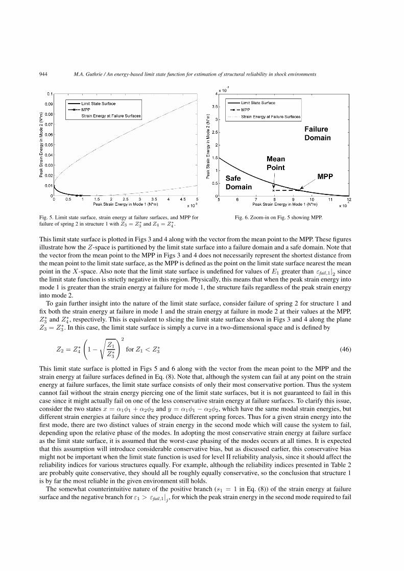
Fig. 5. Limit state surface, strain energy at failure surfaces, and MPP forfailure of spring 2 in structure 1 with Z3 = Z∗

3 and Z4 = Z∗4 .

Fig. 6. Zoom-in on Fig. 5 showing MPP.

This limit state surface is plotted in Figs 3 and 4 along with the vector from the mean point to the MPP. These figuresillustrate how the Z-space is partitioned by the limit state surface into a failure domain and a safe domain. Note thatthe vector from the mean point to the MPP in Figs 3 and 4 does not necessarily represent the shortest distance fromthe mean point to the limit state surface, as the MPP is defined as the point on the limit state surface nearest the meanpoint in the X-space. Also note that the limit state surface is undefined for values of E1 greater than εfail,1|2 sincethe limit state function is strictly negative in this region. Physically, this means that when the peak strain energy intomode 1 is greater than the strain energy at failure for mode 1, the structure fails regardless of the peak strain energyinto mode 2.

To gain further insight into the nature of the limit state surface, consider failure of spring 2 for structure 1 andfix both the strain energy at failure in mode 1 and the strain energy at failure in mode 2 at their values at the MPP,Z∗3 and Z∗

4 , respectively. This is equivalent to slicing the limit state surface shown in Figs 3 and 4 along the planeZ3 = Z∗

3 . In this case, the limit state surface is simply a curve in a two-dimensional space and is defined by

Z2 = Z∗4

(1−√

Z1

Z∗3

)2

for Z1 < Z∗3 (46)

This limit state surface is plotted in Figs 5 and 6 along with the vector from the mean point to the MPP and thestrain energy at failure surfaces defined in Eq. (8). Note that, although the system can fail at any point on the strainenergy at failure surfaces, the limit state surface consists of only their most conservative portion. Thus the systemcannot fail without the strain energy piercing one of the limit state surfaces, but it is not guaranteed to fail in thiscase since it might actually fail on one of the less conservative strain energy at failure surfaces. To clarify this issue,consider the two states x = α1φ1 + α2φ2 and y = α1φ1 − α2φ2, which have the same modal strain energies, butdifferent strain energies at failure since they produce different spring forces. Thus for a given strain energy into thefirst mode, there are two distinct values of strain energy in the second mode which will cause the system to fail,depending upon the relative phase of the modes. In adopting the most conservative strain energy at failure surfaceas the limit state surface, it is assumed that the worst-case phasing of the modes occurs at all times. It is expectedthat this assumption will introduce considerable conservative bias, but as discussed earlier, this conservative biasmight not be important when the limit state function is used for level II reliability analysis, since it should affect thereliability indices for various structures equally. For example, although the reliability indices presented in Table 2are probably quite conservative, they should all be roughly equally conservative, so the conclusion that structure 1is by far the most reliable in the given environment still holds.

The somewhat counterintuitive nature of the positive branch (s1 = 1 in Eq. (8)) of the strain energy at failuresurface and the negative branch for ε1 > εfail,1|j , for which the peak strain energy in the second mode required to fail


Table 5Nominal material properties used in finite element model

Elastic modulus (GPa) Density (kg/m3) Poisson’s ratio Yield stress (MPa)Steel 200 7861 0.30 552Aluminum 68.9 2700 0.33 276

Fig. 7. Drawing of a simple structure consisting of twocircular plates joined by four legs (dimensions in cm).

Fig. 8. Finite element model of structure from Fig. 7.

the structure increases as the peak strain energy in the first mode increases, is the result of a singularity in which themodal displacements produce vanishing force in one of the springs. For example, consider the shape x = α1φ1+φ2

for varying values of α1 and denote the value of α1 for which the force in the first spring vanishes by α1. Then asα1 → α1, the strain energy at failure of the first spring in both modes approaches infinity since the force in the firstspring is vanishing and the scale factor to failure is approaching infinity. Since these branches of the strain energyat failure surface are not included in the definition of the limit state function, they are not considered further in thispaper.

5. Application to a simple finite element model

A more realistic application of the energy-based reliability approach is provided by the structure shown in Fig. 7.This structure consists of two circular plates joined together by four legs with circular cross sections. The base plateis composed of steel while the legs and top plate are composed of aluminum. The nominal properties used for thesematerials are listed in Table 5. A finite element model of this structure consisting of approximately 36,000 8-nodehexahedral elements was constructed and is shown in Fig. 8.

The structure is subjected to the nominal base acceleration shown in Fig. 9 and is considered to have failed ifthe Von Mises stress in any element exceeds the corresponding yield stress. For brevity, only axial (x-direction)shocks are considered here, but the same approach could be used to analyze transverse shocks if desired. Second-moment information for the environmental severity and structural failure characteristics, described here by the peakmodal strain energies and modal strain energies at failure, is assumed to be available and the thickness of the topplate is to be selected in order to maximize the reliability of the structure in the given environment. This problem,although greatly simplified, is representative of many problems frequently encountered in the design of structures forshock environments. In many cases, such problems are addressed simply by analyzing each design for the nominalcase and determining the safety factor. While this approach can provide quick design guidance, it fails to account


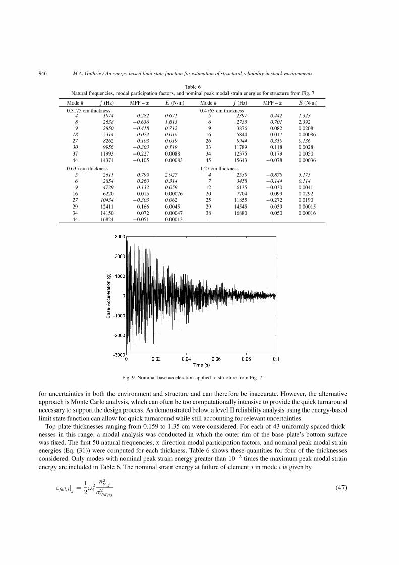
Table 6Natural frequencies, modal participation factors, and nominal peak modal strain energies for structure from Fig. 7

Mode # f (Hz) MPF – x E (N·m) Mode # f (Hz) MPF – x E (N·m)0.3175 cm thickness 0.4763 cm thickness

4 1974 −0.282 0.671 5 2397 0.442 1.3238 2638 −0.636 1.613 6 2735 0.701 2.3929 2850 −0.418 0.712 9 3876 0.082 0.0208

18 5314 −0.074 0.016 16 5844 0.017 0.0008627 8262 0.103 0.019 26 9944 0.310 0.13630 9956 −0.303 0.119 33 11789 0.118 0.002837 11993 −0.227 0.0088 34 12375 0.179 0.005044 14371 −0.105 0.00083 45 15643 −0.078 0.00036

0.635 cm thickness 1.27 cm thickness5 2611 0.799 2.927 4 2539 −0.878 5.1756 2854 0.260 0.314 7 3458 −0.144 0.1149 4729 0.132 0.059 12 6135 −0.030 0.0041

16 6220 −0.015 0.00076 20 7704 −0.099 0.029227 10434 −0.303 0.062 25 11855 −0.272 0.019029 12411 0.166 0.0045 29 14545 0.039 0.0001534 14150 0.072 0.00047 38 16880 0.050 0.0001644 16824 −0.051 0.00013 – – – –

Fig. 9. Nominal base acceleration applied to structure from Fig. 7.

for uncertainties in both the environment and structure and can therefore be inaccurate. However, the alternativeapproach is Monte Carlo analysis, which can often be too computationally intensive to provide the quick turnaroundnecessary to support the design process. As demonstrated below, a level II reliability analysis using the energy-basedlimit state function can allow for quick turnaround while still accounting for relevant uncertainties.

Top plate thicknesses ranging from 0.159 to 1.35 cm were considered. For each of 43 uniformly spaced thick-nesses in this range, a modal analysis was conducted in which the outer rim of the base plate’s bottom surfacewas fixed. The first 50 natural frequencies, x-direction modal participation factors, and nominal peak modal strainenergies (Eq. (31)) were computed for each thickness. Table 6 shows these quantities for four of the thicknessesconsidered. Only modes with nominal peak strain energy greater than 10−5 times the maximum peak modal strainenergy are included in Table 6. The nominal strain energy at failure of element j in mode i is given by

εfail,i|j =1

2ω2i

σ2Y,j

σ2VM,ij

(47)


Table 7Sensitivity vectors for structure of Fig. 7

0.3175 cm thickness 0.4763 cm thickness 0.635 cm thickness 1.27 cm thicknessE4 −0.158 E5 −0.090 E5 −0.464 E4 −0.576E8 −0.175 E6 −0.035 E6 −0.094 E7 −0.036E9 −0.109 E9 −0.008 E9 −0.034 E20 −0.015E30 −0.013 E26 −0.020 E27 −0.030 E25 −0.015εfail,4 0.315 εfail,5 0.559 εfail,5 0.644 εfail,4 0.735εfail,8 0.348 εfail,6 0.211 εfail,6 0.120 εfail,7 0.042εfail,9 0.217 εfail,9 0.049 εfail,9 0.043 εfail,20 0.018εfail,30 0.026 εfail,26 0.122 εfail,27 0.037 εfail,25 0.018

where σY,j is the nominal yield stress for element j and σVM,ij is the Von Mises stress in element j for mass-normalized mode i. Note that, because Von Mises stress is not a linear function of displacement, it does not satisfythe assumptions underlying the limit state function. Nonetheless, it is still used to define failure for this structureand the resulting reliability indices agree well with Monte Carlo analysis, so it appears that this inconsistency doesnot have a large effect on the accuracy. Future work will examine the error introduced by this assumption morequantitatively.

For each of the elements, the vector of basic variables is given in Eq. (16) and the limit state function and itsgradient are given in Eqs (17) and (24). For each candidate thickness and each element, the expected value of Z canbe evaluated using Eqs (31) and (47). Each basic variable is assigned a coefficient of variation equal to 0.5 exceptfor the modal strain energies at failure for the elements in the top plate, which are given coefficients of variationequal to 1.0. This corresponds to a situation in which there is greater uncertainty in the yield stress of the top platethan in that of the other components, as might be the case if the top plate is produced by a different supplier. Giventhe assumptions about the correlation between the basic variables discussed earlier, the covariance matrix for Z canbe evaluated. The iterative procedure given in Eq. (23) was applied to find the MPP, and hence the Hasofer-Lindreliability index, for each of the candidate thicknesses. The reliability index, along with the reliability indices forthe top plate, base plate, and legs, is plotted as a function of top plate thickness in Fig. 10. The sensitivity vectorfrom Eq. (27) is given in Table 7 for four values of the top plate thickness. To ensure that the 50 modes includedin the computation were sufficient to obtain converged values of the reliability index, the number of modes shapeswas increased to 100 for thicknesses of 0.3175, 0.4763, 0.635, and 1.27 cm. In these four cases, the reliability indexchanged by a maximum of 6.6%, which was deemed to be a sufficient level of convergence. In addition to doublingthe number of mode shapes, standard rules of thumb such as including modes with natural frequencies up to twicethe maximum frequency of the input can be used to determine an appropriate number of modes. For comparisonwith the reliability indices, a modal transient analysis of the nominal case (i.e., yield stresses from Table 5 and baseacceleration from Fig. 9) was performed for each candidate thickness and the safety factor was calculated as

SF = mini

σY,i

σVM,i(48)

where i ranges from 1 to the number of elements and σVM,i represents the peak Von Mises stress in element i over alltime steps. The safety factors computed in this way are plotted as a function of top plate thickness in Fig. 11, alongwith the safety factors for the top plate, base plate, and legs. In the modal transient analyses, the first 50 modes wereretained, a timestep of 10−6 s was used, the base acceleration from Fig. 9 was enforced along the outer rim of thebottom surface of the base plate, and the response was integrated over 300 ms.

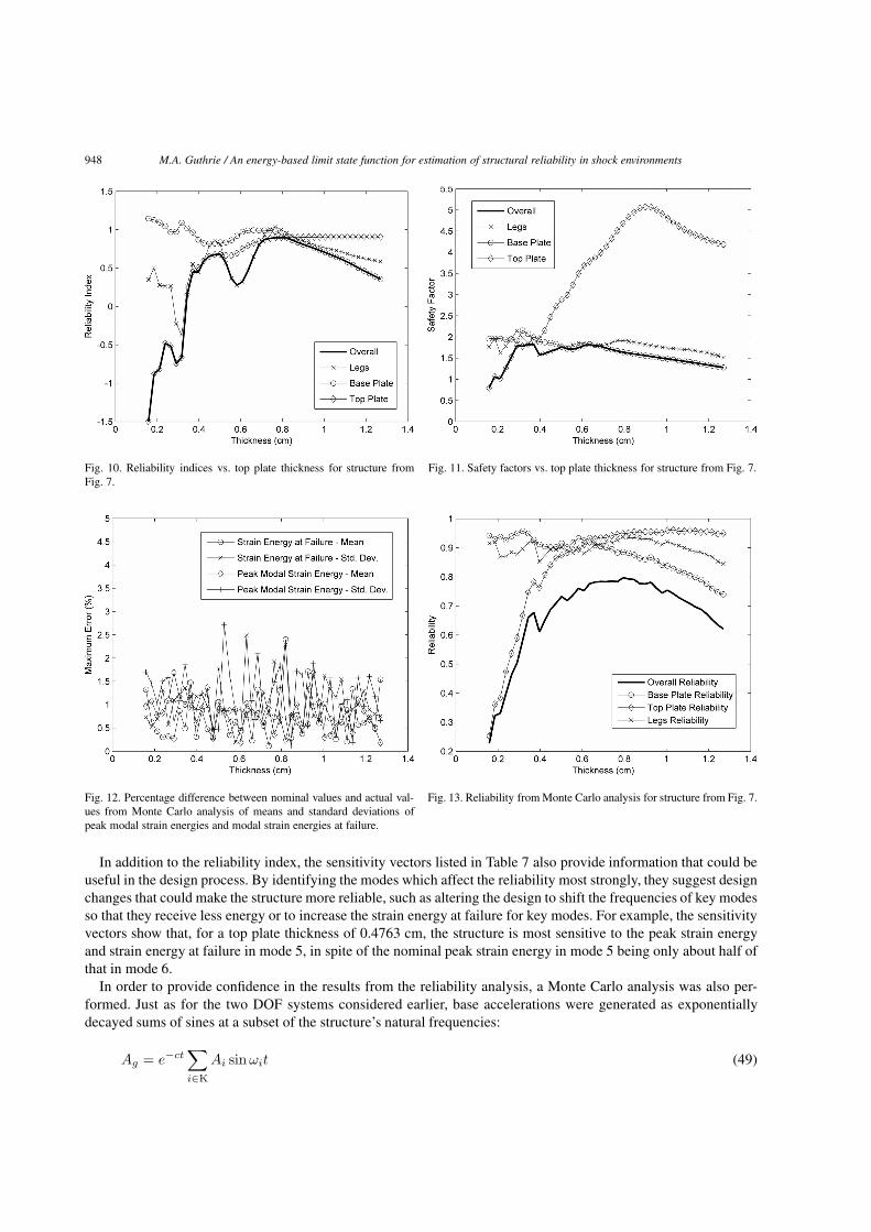
The reliability indices from Fig. 10 suggest that increasing the thickness of the top plate from 0.159 cm to 0.82 cmgenerally increases the reliability of the structure, although there are a few local minima in the reliability indexaround 0.3, 0.4, and 0.6 cm. For thicknesses from 0.159 to 0.82 cm, the minimum reliability index is associated withthe top plate, except for thicknesses between 0.50 and 0.71 cm, for which the minimum reliability index is associatedwith the legs. As the thickness is increased beyond 0.82 cm, the minimum reliability index is associated with thebase plate and the reliability is reduced for further increases in the thickness. The reliability index is maximized ata top plate thickness of 0.82 cm. By comparison, the safety factors from Fig. 11 are maximized at a thickness of0.37 cm. The discrepancy between the safety factors and the reliability indices is a result of the safety factor notaccounting for variation in both the structure and the environment.


Fig. 10. Reliability indices vs. top plate thickness for structure fromFig. 7.

Fig. 11. Safety factors vs. top plate thickness for structure from Fig. 7.

Fig. 12. Percentage difference between nominal values and actual val-ues from Monte Carlo analysis of means and standard deviations ofpeak modal strain energies and modal strain energies at failure.

Fig. 13. Reliability from Monte Carlo analysis for structure from Fig. 7.

In addition to the reliability index, the sensitivity vectors listed in Table 7 also provide information that could beuseful in the design process. By identifying the modes which affect the reliability most strongly, they suggest designchanges that could make the structure more reliable, such as altering the design to shift the frequencies of key modesso that they receive less energy or to increase the strain energy at failure for key modes. For example, the sensitivityvectors show that, for a top plate thickness of 0.4763 cm, the structure is most sensitive to the peak strain energyand strain energy at failure in mode 5, in spite of the nominal peak strain energy in mode 5 being only about half ofthat in mode 6.

In order to provide confidence in the results from the reliability analysis, a Monte Carlo analysis was also per-formed. Just as for the two DOF systems considered earlier, base accelerations were generated as exponentiallydecayed sums of sines at a subset of the structure’s natural frequencies:

Ag = e−ct∑i∈K

Ai sinωit (49)


Fig. 14. Overlay of reliability index and Monte Carlo reliability vs. topplate thickness.

Fig. 15. Overlay of safety factor and Monte Carlo reliability vs. topplate thickness.

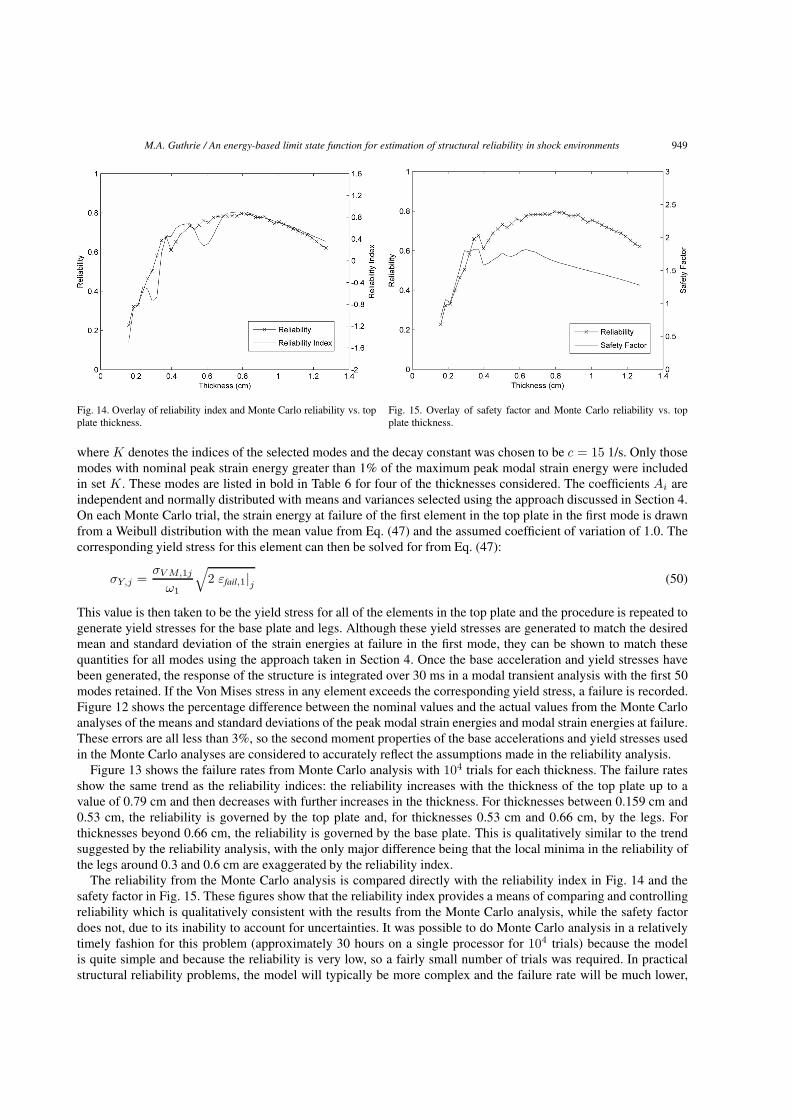
where K denotes the indices of the selected modes and the decay constant was chosen to be c = 15 1/s. Only thosemodes with nominal peak strain energy greater than 1% of the maximum peak modal strain energy were includedin set K . These modes are listed in bold in Table 6 for four of the thicknesses considered. The coefficients Ai areindependent and normally distributed with means and variances selected using the approach discussed in Section 4.On each Monte Carlo trial, the strain energy at failure of the first element in the top plate in the first mode is drawnfrom a Weibull distribution with the mean value from Eq. (47) and the assumed coefficient of variation of 1.0. Thecorresponding yield stress for this element can then be solved for from Eq. (47):

σY,j =σV M,1j

ω1

√2 εfail,1|j (50)

This value is then taken to be the yield stress for all of the elements in the top plate and the procedure is repeated togenerate yield stresses for the base plate and legs. Although these yield stresses are generated to match the desiredmean and standard deviation of the strain energies at failure in the first mode, they can be shown to match thesequantities for all modes using the approach taken in Section 4. Once the base acceleration and yield stresses havebeen generated, the response of the structure is integrated over 30 ms in a modal transient analysis with the first 50modes retained. If the Von Mises stress in any element exceeds the corresponding yield stress, a failure is recorded.Figure 12 shows the percentage difference between the nominal values and the actual values from the Monte Carloanalyses of the means and standard deviations of the peak modal strain energies and modal strain energies at failure.These errors are all less than 3%, so the second moment properties of the base accelerations and yield stresses usedin the Monte Carlo analyses are considered to accurately reflect the assumptions made in the reliability analysis.

Figure 13 shows the failure rates from Monte Carlo analysis with 104 trials for each thickness. The failure ratesshow the same trend as the reliability indices: the reliability increases with the thickness of the top plate up to avalue of 0.79 cm and then decreases with further increases in the thickness. For thicknesses between 0.159 cm and0.53 cm, the reliability is governed by the top plate and, for thicknesses 0.53 cm and 0.66 cm, by the legs. Forthicknesses beyond 0.66 cm, the reliability is governed by the base plate. This is qualitatively similar to the trendsuggested by the reliability analysis, with the only major difference being that the local minima in the reliability ofthe legs around 0.3 and 0.6 cm are exaggerated by the reliability index.

The reliability from the Monte Carlo analysis is compared directly with the reliability index in Fig. 14 and thesafety factor in Fig. 15. These figures show that the reliability index provides a means of comparing and controllingreliability which is qualitatively consistent with the results from the Monte Carlo analysis, while the safety factordoes not, due to its inability to account for uncertainties. It was possible to do Monte Carlo analysis in a relativelytimely fashion for this problem (approximately 30 hours on a single processor for 104 trials) because the modelis quite simple and because the reliability is very low, so a fairly small number of trials was required. In practicalstructural reliability problems, the model will typically be more complex and the failure rate will be much lower,


perhaps on the order of one-in-a-million, so a much larger number of trials will be required. While Monte Carloanalysis might still be possible in some of these cases, it would require substantial computational resources andtime. In situations where quick, qualitative comparison of several designs is required, such an approach would betoo slow and inflexible. The use of level II reliability analysis with the energy-based limit state function provides analternative approach which requires only a modal analysis and some simple post-processing of the results, but stillaccounts for relevant uncertainties in the structure and environment. In addition, it provides valuable informationabout the spectral sensitivity of the reliability.

6. Conclusion

A limit state function based upon the peak modal strain energies and modal strain energies at failure has beendeveloped for the estimation of structural reliability in shock environments. The Hasofer-Lind reliability index wasbriefly reviewed and it was shown how this index can be computed for the energy-based limit state function. LevelII reliability analysis using the energy-based limit state function was performed for two DOF mass-spring systemsand a simple finite element model and, in both cases, the results were seen to agree well with those from MonteCarlo analysis.

The reliability index for the energy-based limit state function provides an accurate and easily calculated measureof a structure’s reliability. Use of this index could be very valuable during the design process, when fast, qualita-tive comparison of the relative reliabilities of various design options is required. In such situations, Monte Carloanalysis is often too computationally intensive to provide the fast turnaround required to support design studies.The reliability approach developed here requires little effort beyond a modal analysis, but still accounts for relevantuncertainties in both the structure and environment. In addition, the reliability approach developed here providesimportant information about the sensitivity of the structure’s reliability to the frequency content of the input.

Acknowledgments

Sandia National Laboratories is a multi-program laboratory managed and operated by Sandia Corporation, awholly owned subsidiary of Lockheed Martin Corporation, for the U.S. Department of Energy’s National NuclearSecurity Administration under contract DE-AC04-94AL85000. The author would also like to acknowledge the im-portant contributions of Tim Edwards to this work, both in developing the energy-based characterization of shockand vibration environments and in encouraging its extension to the prediction of structural reliability.

References

[1] D.E. Hudson, Response spectrum techniques in engineering seismology, Proceedings of the World Conference on Earthquake Engineering,Berkeley, California, (1956), 4–1, 4–12.

[2] G.W. Housner, Behavior of structures during earthquake, Journal of the Engineering Mechanics Division (ASCE) 85(4) (1959), 109–129.[3] G.W. Housner, Limit design of structures to resist earthquakes, Proceedings of the World Conference on Earthquake Engineering, Berkeley,

California, (1956), 5–1, 5–13.[4] T.S. Edwards, Power delivered to mechanical systems by random vibrations, Shock and Vibration 16(3) (2009), 261–271.[5] T.S. Edwards, Using work and energy to characterize mechanical shock, Technical Report SAND2007-0851J, Sandia National Laborato-

ries, Albuquerque, NM, February 2007.[6] T.S. Edwards, D.O. Smallwood and D.J. Segalman, Modal deposition of shock energy, Technical Report SAND2007-0691J, Sandia Na-

tional Laboratories, Albuquerque, NM, February 2007.[7] H.O. Madsen, S. Krenk and N.C. Lind, Methods of structural safety, Dover Publications, Mineola, NY, 1986.[8] P. Thoft-Christensen and M.J. Baker, Structural reliability theory and its applications, Springer-Verlag, Berlin, 1982.[9] A.M. Hasofer and N.C. Lind, Exact and invariant second-moment code format, Journal of the Engineering Mechanics Division (ASCE)

100 (1974), 111–121.[10] C.A. Cornell, A probability-based structural code, Journal of the American Concrete Institute 66(12) (1969), 974–985.

International Journal of

AerospaceEngineeringHindawi Publishing Corporationhttp://www.hindawi.com Volume 2010

RoboticsJournal of

Hindawi Publishing Corporationhttp://www.hindawi.com Volume 2014


Active and Passive Electronic Components

Control Scienceand Engineering

Journal of



RotatingMachinery


Hindawi Publishing Corporation http://www.hindawi.com

Journal ofEngineeringVolume 2014

Submit your manuscripts athttp://www.hindawi.com

VLSI Design



Shock and Vibration


Civil EngineeringAdvances in

Acoustics and VibrationAdvances in



Electrical and Computer Engineering

Journal of

Advances inOptoElectronics

Hindawi Publishing Corporation http://www.hindawi.com

Volume 2014

The Scientific World JournalHindawi Publishing Corporation http://www.hindawi.com Volume 2014

SensorsJournal of


Modelling & Simulation in EngineeringHindawi Publishing Corporation http://www.hindawi.com Volume 2014


Chemical EngineeringInternational Journal of Antennas and

Propagation




Navigation and Observation



DistributedSensor Networks


An energy-based limit state function for estimation of ...

Documents

Transcript of An energy-based limit state function for estimation of ...