An energy-aware survey on ICT device power supplies

Printed in SwitzerlandGeneva, 2012

Photo credits: Shutterstock®

About ITU-T and Climate Change: itu.int/ITU-T/climatechange/E-mail: greenstandard@itu.int

September 2012!"#"$%&&'()$*+%(,-."/0%1,-*(2-

-------!"#"&*+$,-3*4%1*/%15-

6.789:;7!<-=9>37-;!6=7-=7->9.?8@-

.*+%(*#-7(/"1A6()B"1,)/5-C%(,%1+'&-D%1-!"#"$%&&'()$*+%(,--

About GeSI: www.gesi.orgE-mail: info@gesi.org

Acknowledgements

This report was commissioned by the Global e-Sustainability Initiative (GeSI) and International Telecommunication Union to Raffaele Bolla, Roberto Bruschi and Luca D’Agostino (University of Genoa, Italy).

The report has benefited from the input and comments of many people to whom we owe our thanks. Among others, Flavio Cucchietti (Telecom Italia), the members of the GeSI Energy Efficiency Working Group listed below, Luca Giacomello (Telecom Italia), Cristina Bueti and Matthew Dalais (ITU). Special thanks goes to the strong support offered by Bertana S.r.l for the electrical measurements, for the collaboration of the Trony/Gallenca shop (Via Gorizia, Turin) in giving access to a large number of commercial devices, the Telecom Italia Lab staff for the willingness to make their home adapters available for the measurements and especially to the Politecnico di Torino for the LCA analysis.

Members of GeSI Energy Efficiency Working Group: Gilbert Buty (Alcatel-Lucent), Raj Kumar (Amdocs), John Messina (AT&T), Steve Bernard (AT&T), Roman Smith (AT&T), Shannon Carroll (AT&T), Gabrielle Giner (BT), Mark Shackleton (BT), Andreas Kröhling (Deutsche Telekom AG), Karl-Heinz Reckman (Deutsche Telekom AG), Johann Kiendl (Deutsche Telekom), Susanne Lundberg (Ericsson), Jens Malmodin (Ericsson), Elaine Weidman (Ericsson), Ylva Jading (Ericsson), Alice Valvodova (GeSI), Veronica Cooper (GeSI), Christopher Wellise (Hewlett Packard), Christopher Librie (Hewlett Packard), Maria Morse (Hewlett Packard), Paolo Gemma (Huawei), Bin Zhu (Huawei), Francisco Da Silva (Huawei), Cristina Bueti (ITU), Marga Blom (KPN), Hans Devries (KPN), Theresa Jordan (Motorola Solutions), Dominique Roche (Orange France Telecom Group), Ahmed Zeddam (Orange France Telecom Group), Katerina Perissi (OTE), Kyriaki Zannia (OTE), Parasoglou Kyriakos (OTE), Koukouselis Ioannis (OTE), Despina Komninou (OTE), Gianluca Griffa (Telecom Italia), Flavio Cucchietti (Telecom Italia), Daniela Torres (Telefonica), Gabriel Bonilha (Telefonica), Jan Kristensen (Telenor), Harald Birkeland (Telenor), Geir Millstein (Telenor), Aytac Soysevener (Turk Telecom), Tugba Gur (Turk Telecom), Howard Davis (Verizon), Nicola Woodhead (Vodafone), Joe Griffin (Vodafone), Lucy Connell (Vodafone), Shi Qingfei (ZTE).

Additional information and materials relating to this Report can be found at: www.itu.int/itu-t/climatechange www.gesi.org

If you would like to provide any additional information, please contact: Cristina Bueti at greenstandard@itu.int Alice Valvodova at alice.valvodova@gesi.org

Legal Notice

This publication may be updated from time to time.

Third-party sources are quoted as appropriate. The International Telecommunication Union (ITU) and the Global e-Sustainability Initiative (GeSI) are not responsible for the content of external sources including external websites referenced in this publication.

Disclaimer

The views expressed in this publication are those of the authors and do not necessarily reflect the views of the International Telecommunication Union (ITU) and of the Global e-Sustainability Initiative (GeSI).

Mention of and references to specific countries, companies, products, initiatives or guidelines do not in any way imply that they are endorsed or recommended by ITU, the authors, or any other organization that the authors are affiliated with, in preference to others of a similar nature that are not mentioned.

Requests to reproduce extracts of this publication may be submitted to: jur@itu.int and info@gesi.org

© ITU and GeSI 2012

All rights reserved. No part of this publication may be reproduced, by any means whatsoever, without the prior written permission of ITU and GeSI.

i

Table of contents

Page

Foreword ................................................................................................................................................. iii

1. Executive summary ............................................................................................................................ 1

1.1 Introduction ........................................................................................................................................1

1.2 Report structure and main outcomes ................................................................................................1

2. Classification and category definition ................................................................................................ 3

3. Nameplate data ................................................................................................................................. 6

4. Mechanical features ........................................................................................................................ 20

4.1 Weight ............................................................................................................................................. 20

4.2 Volume ............................................................................................................................................. 24

4.3 Power density .................................................................................................................................. 26

4.4 Estimation on use of resources and e-waste ................................................................................... 27

5. Electrical features ............................................................................................................................ 28

5.1 Efficiency measurements ................................................................................................................. 28 5.1.1 Efficiency measurements – subdivided per-class .................................................................... 29 5.1.2 Efficiency at lower load – impact on some products ............................................................... 38 5.1.3 Power factor vs. load and efficiency ........................................................................................ 39

5.2 Correlation between safety class and efficiency ............................................................................. 42

5.3 Replicability of the efficiency behaviour ......................................................................................... 43

5.4 Analytical analysis ............................................................................................................................ 44

5.5 Output voltage ................................................................................................................................. 50

5.6 No-load ............................................................................................................................................ 57

6. Mass balance and environmental considerations ............................................................................. 60

6.1 Global Warming Potential, GWP...................................................................................................... 60

7. Conclusion ....................................................................................................................................... 61

8. References ....................................................................................................................................... 63

9. Appendix A ...................................................................................................................................... 64

9.1 Test bed ............................................................................................................................................ 64

10. Appendix B – LIFE CYCLE ASSESSMENT METHODOLOGY APPLIED TO POWER SUPPLIES FOR CUSTOMER PREMISES EQUIPMENT * ............................................................................................... 65

Foreword

iii

ITU is committed to working in partnership with organizations around the world to produce global policies and standards to tackle climate change and environmental degradation.

This report reveals that standards for the manufacture of external power supplies (EPS) could enhance their reliability and extend their lifetime while decreasing their average weight by up to 30 per cent. This could eliminate up to sixty per cent of current annual EPS e-waste.

In addition the report highlights that standardizing efficiency characteristics could reduce the energy consumption and greenhouse gas (GHG) emissions of EPSs by between 25 and 50 per cent.

ICT users and manufacturers are already enjoying the economic and environmentalbenefits of the ITU Universal Charger detailed in Recommenda-tion ITU-T L.1000. ITU-T Study Group 5 – ITU’s lead study group on environment and climate change – is now building on this success with new standards applicable to a wider range of ICTs.

This new report on the results of “An energy-aware survey on ICT device power supplies” firmly underlines opportunities to achieve further reductions in e-waste, energy use and greenhouse gas emissions; and the resultant ITU-T Recommendations will achieve this by widening the range of ICTs supported by power adaptors and standardizing design parameters able to optimize these adaptors’ eco-efficiency.

Malcolm Johnson, Director, Telecommunication Standardization Bureau, ITU

The Global e-Sustainability Initiative (GeSI) has been participating in the global debate on sustainable development for over a decade. The rapid deployment of innovative ICT solutions must be matched with a commitment to create environmentally responsible products that are energy efficient, reduce the carbon footprint of the ICT sector and meet consumer needs.

This report marks another milestone in GeSI’s role of bringing together leading ICT companies and international organisations to raise awareness of the contribution of innovative technology to sustainability. Commissioned by GeSI and ITU, it presents the results of a study of more than 300 commercially available adapters, both for ICT and non-ICT use. The report suggests that an environmentally friendly design could result in savings of more than 30 per cent of the materials used to build the devices. Avoiding obsolescence would cut down on the 300,000 tons of e-waste likely to be created per year by discarded devices. In addition, the report highlights that standardising efficiency characteristics could reduce the energy consumption and greenhouse gas emissions of power supplies by between 25 and 50 per cent.

On behalf of GeSI, I urge all manufacturers and telecommunication service providers to review this report and focus their efforts on improving energy efficiency wherever possible. Together with our stakeholders, GeSI aims to fulfil its mission of building a responsible world through ICT-enabled transformation. Join us in driving the sustainability agenda.

Luis Neves, GeSI Chairman

1

An energy-aware survey on ICT device power supplies

1. Executive summary

1.1 Introduction

This report presents the results of a study commissioned by the International Telecommunication Union (ITU) and the Global e-Sustainability Initiative (GeSI). The study analysed over 300 commercially-available External Power Supplies (EPSs) – devices both within and outside the ambit of information and communication technology (ICT) – with a view to providing input to the standardization activity of ITU-T Study Group 5 (Environment and climate change).

Decreasing the life-cycle environmental impact of EPSs is an exceptionally important part of efforts to ‘green’ the ICT sector, and the results of this study will inform work taking place within ITU-T Study Group 5 on phase two of the very successful ITU Universal Charging Solution – Recommendation ITU-T L.1000: Universal power adapter and charger solution for mobile terminals and other hand-held ICT devices.

Considering only the EPSs within the scope of this study, 4 billion new EPSs will be sold in 2012; a figure predicted to increase by 12 per cent annually. If not reasonably energy-efficient, they will consume unnecessarily large quantities of energy; and if not repairable in the case of failure, not (at least partially) recyclable, or not designed to be used with more than one type of device, large volumes of EPSs will find their way to landfill and become part of an escalating e-waste challenge.

Looking at 2014’s projected EPS sales, enhancing the energy efficiency of each EPS by as little as 1 Watt would achieve energy savings in the region of 1.8 Tera-Watts per hour (assuming an average usage of 1 hour per day). Additionally, the average weight of an EPS is around 250 grams and, if half of the EPSs sold in 2014 replace those disposed of, EPSs will in that year be responsible for 600,000 tons of e-waste.

1.2 Report structure and main outcomes

The report is composed of two main sections.

1) In sections 2 and 3, EPSs are classified, analysed and compared on the basis of their electrical (voltage, power, current, efficiency class, etc.) and physical characteristics (e.g., weight, volumes, mains and DC voltage connector type).

The results of this analysis give clear indications of a tendency towards “de facto” standards (e.g. output voltages, connector types), and highlight significant opportunities to improve EPSs’ eco-efficiency through, for instance, large weight-reduction opportunities associated with the majority of EPSs analysed.

2) Sections 4 and 5 analyse the energy efficiency of surveyed EPSs.

The results strongly indicate that the efficiency of many EPSs is well below the optimum level, both in terms of dynamic behaviour (i.e., when providing electrical current to the attached devices) and in terms of the “no load condition” (i.e., when EPSs are connected to the energy grid, but not providing energy to the attached devices).

2

The study’s findings can be summarized as follows:

a) Optional energy-efficiency regulations are neglected

The Energy Star Program (www.eu-energystar.org/en/index.html), sponsored by the US Government and the European Union (EU), defines energy-efficiency classes and the associated labelling for consumer products. However, only 47 per cent of the analysed EPSs are marked with the Energy Star label and this label is rarely present in the more widespread lower-power adapters; suggesting the presence of efficiency shortfalls in many of the EPSs analysed.

b) Common practices signify the existence of de-facto standards

Voltage, current and power values tend towards common ratings, signifying partial “de facto” standardization. This condition is particularly evident in two specific aspects: The low-voltage connectors: the five most-used connector types represent 86% of the total The output voltage: 81% of the devices have an output voltage equal to 5 V, 12 V or 19 V.

c) Potential improvements: Possible benefits of standardization Improving Usability

• Different connectors for different output voltages Power supplies with very different output voltages often make use of the same type of connector. This situation creates confusion and implies a risk to consumers attempting to use the same EPS to charge products with different input-voltage requirements. The standardization of a set of connectors and output voltages should be considered, as should a standardization of the constraints linking these items.

• Replaceable cables The main cause of failure in all power supplies is a weak point where the low-voltage cable is connected to the power supply. This weak point confirms the need for connectors standardized according to different voltage and current requirements, and it is highly recommended that EPSs provide a detachable, replaceable cable on the low-voltage side of the device.

• Accuracy of tag information Certain adapters were found to produce an output voltage higher than that declared by the supplier and reported on their nameplate. This would understandably lead to difficulties when using the same EPS to charge devices with different requirements.

Design optimization to improve eco-sustainability

• Reduce EPS size Despite having the same electrical characteristics (voltage and power), EPSs produced by different vendors often possess very different physical dimensions (weight and volume). In most EPS categories, a large proportion of EPSs weigh over 20% more than the category’s lightest EPS. Weight is directly linked to environmental impact, and manufacturers should be urged to align their products with “best-practice” EPS dimensions.

• Increase power efficiency Measurements taken in the study uncover large power-efficiency variations among items with comparable electrical characteristics; underlining a key opportunity to improve average efficiency. Comparable EPSs display varying power-efficiency levels in “low-load” and “no-load” conditions (i.e., when the supplied device requires 10-30 per cent of the maximum power, or when it is switched-off while the power supply is still connected to the electricity grid). Standards aligning the low-load power efficiencies of EPSs would therefore translate into significant energy savings.

• Standardized design rules The study considers items from two different “safety classes”: Class 1 (grounded, 3-pronged mains connector) and Class 2 (2-pronged mains connector). Roughly 65 per cent of the surveyed EPSs belong to Class 2, which is the more stringent of the two classes. Measurements taken in the study

3

indicate that devices belonging to Class 2 are superior to devices in Class 1 with regard to their power efficiency and ratio of weight to supplied power. Class 2 devices also guarantee greater protection from energy grid overvoltages, and a strong case can be made for the adoption of Class 2 as the standardized solution for external power supplies as its 2-prong mains connector would allow compatibility with most country-specific mains receptacles located where ground is not available.

2. Classification and category definition

Due to the large amount of the different types of the both power supplies and the corresponding powered devices, a set of categories with different electrical characteristics has been defined. This subdivision allows a better analysis of the large quantity of data and measurements acquired and, moreover, it allows a better comparison among the different devices. The classification is based on three different main electrical characteristics: output voltage (V), output maximum current (I) and maximum power (W). The first subdivision has been done by using the output voltage, i.e., four separate groups have been identified: under 12V, 12V, between 12V and 18V and over 18V. The two groups 12V and above 18V have been further subdivided: the first one into three categories by using the output maximum current, and the second one into four categories by using the power. The following ten categories are the final results of the classification:

1. Category A: Voltage < 12 V, Current: any, Power: any;

2. Category B: Voltage = 12V, Current ≤ 1 A, Power: any;

3. Category C: Voltage = 12V, 1 A < Current ≤ 2 A, Power: any;

4. Category D: Voltage = 12V, 2 A < Current ≤ 3.5 A, Power: any;

5. Category E: Voltage = 12V, 3.5 A < Current ≤ 5 A, Power: any;

6. Category F: 12V < Voltage < 18V, Current: any, Power: any;

7. Category G: Voltage ≥ 18V, Current: any, Power ≤ 45W;

8. Category H: Voltage ≥ 18V, Current: any, 45W < Power ≤ 70 W;

9. Category I: Voltage ≥ 18V, Current: any, 70W < Power ≤ 95W;

10. Category J: Voltage ≥ 18V, Current: any, 95W < Power ≤ 120 W;

As a first attempt, to verify the relative impact of the above-mentioned categories with respect to the equipment offered on the market, a preliminary analysis based on the most recent power supply data list released by the Energy Star Program (ESP) has been realized. The used reference document is named “External Power Supplies AC-DC Product List; December 16, 2010”. This document is a sheet which originally lists 3782 models of power supplies including the chargers for mobile devices, and it reports, inter alia, the nameplate electrical characteristics, the no-load efficiency, the average active efficiency and the power factor for all the models. This group of devices has been filtered to exclude the mobile chargers and the very low load power external power supplies (EPSs) (not part of this analysis to avoid overlap between L.1000 and L.adapter.phase2)) by limiting the considered elements to those fulfilling both the following parameters:

• Output voltage > 6V and maximum power > 4,5W, or

• Output voltage = 5V and maximum output power > 7,5 W

The resulting filtered list has 2743 different models. Figure 1 shows the numerical and percentage impact on the total of all the different categories1 in this list.

1 Note that, 170 devices of the ESP list do not belong to any defined categories.

4

Generally speaking, these data cannot directly represent the numerical impact on the market, because the list has an entry for each model without the corresponding market volume. Public commercial data (e.g., sold units per models) are not available; however, considering the large number of analyzed models, the result has a statistical relevance with respect to the real market, as confirmed by the collected data and our experience.

Figure 1: Numerical and percentage impact of the different defined categories with respect to the filtered ESP device list.

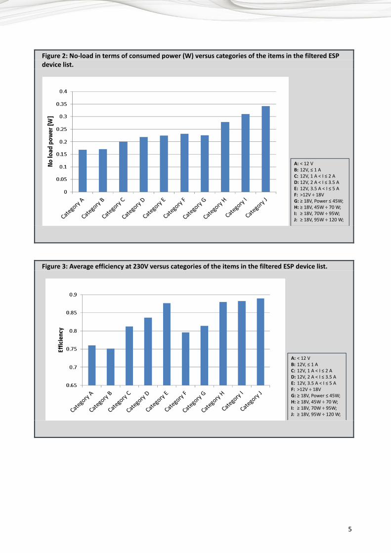
Together with the numerical impact, the average electrical characteristics for each category have also been extracted and reported by means of a graphical representation. The following Figure 2 and Figure 3 report the no-load power consumption and the average efficiency (at 230 V), respectively, averaged on each category and for all the items in the filtered ESP list. These values will be compared in the following sections with those directly measured during this study. Note that these data include all the list of devices and not only the devices with a specific Energy Star rate.

A: < 12 V B: 12V, ≤ 1 A C: 12V, 1 A < I ≤ 2 A D: 12V, 2 A < I ≤ 3.5 A E: 12V, 3.5 A < I ≤ 5 A F: >12V ÷ 18V G: ≥ 18V, Power ≤ 45W; H: ≥ 18V, 45W ÷ 70 W; I: ≥ 18V, 70W ÷ 95W; J: ≥ 18V, 95W ÷ 120 W;

5

Figure 2: No-load in terms of consumed power (W) versus categories of the items in the filtered ESP device list.

Figure 3: Average efficiency at 230V versus categories of the items in the filtered ESP device list.

A: < 12 V B: 12V, ≤ 1 A C: 12V, 1 A < I ≤ 2 A D: 12V, 2 A < I ≤ 3.5 A E: 12V, 3.5 A < I ≤ 5 A F: >12V ÷ 18V G: ≥ 18V, Power ≤ 45W; H: ≥ 18V, 45W ÷ 70 W; I: ≥ 18V, 70W ÷ 95W; J: ≥ 18V, 95W ÷ 120 W;

A: < 12 V B: 12V, ≤ 1 A C: 12V, 1 A < I ≤ 2 A D: 12V, 2 A < I ≤ 3.5 A E: 12V, 3.5 A < I ≤ 5 A F: >12V ÷ 18V G: ≥ 18V, Power ≤ 45W; H: ≥ 18V, 45W ÷ 70 W; I: ≥ 18V, 70W ÷ 95W; J: ≥ 18V, 95W ÷ 120 W;

6

3. Nameplate data

This section reports the results of an analysis performed on the set of 307 external power supplies from various brands. This is a quite large number of devices especially considering the great effort needed to analyze each unit. Moreover, this number is definitely larger than the target one we have define at the beginning of the work, it makes the analysis statistically representative and it has been fixed only by the availability of time and the availability of devices to test. The analyzed adapters were selected in order to cover a wide range of output power (from 1W to more than 170W) while representing a different set from the USB range covered by Recommendation ITU-T L.1000. Note that only the fixed output, single voltage adapters have been considered.

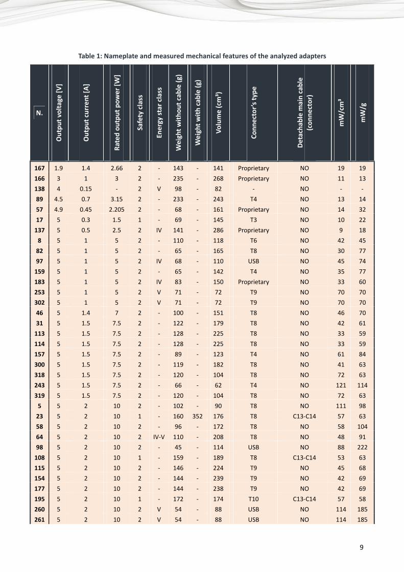
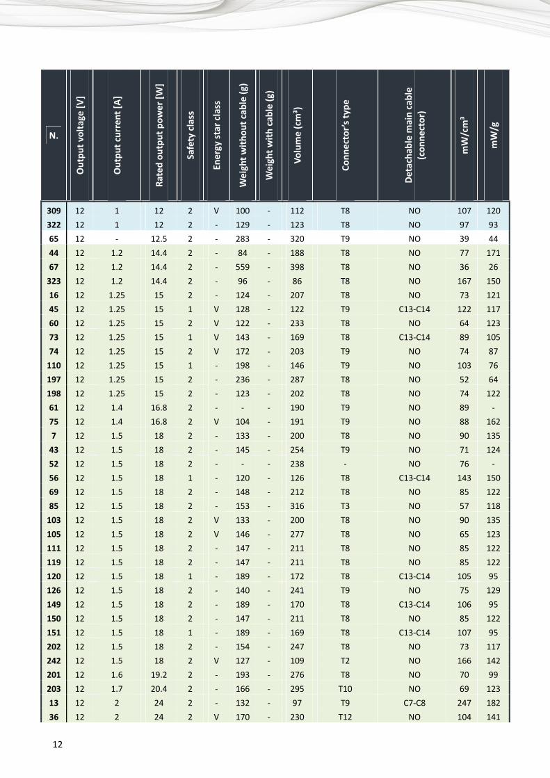
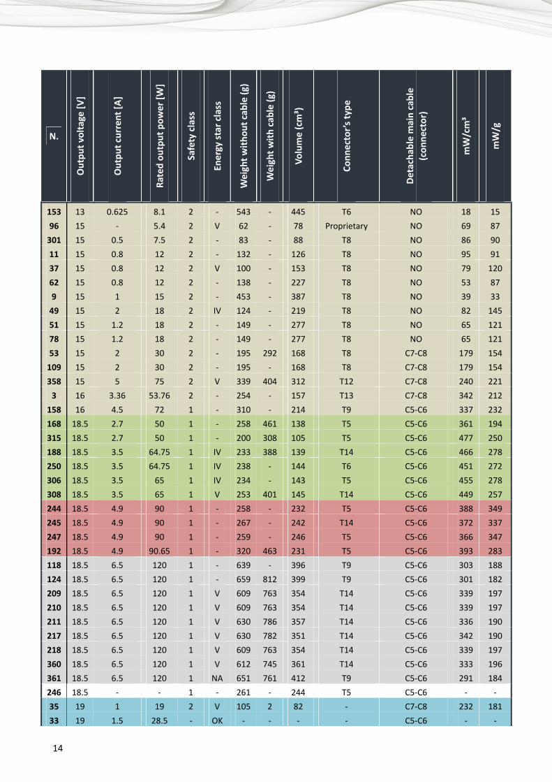
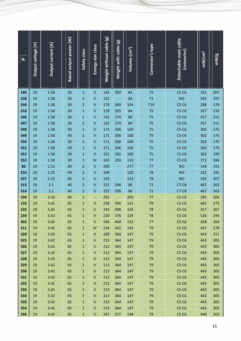
Table 1 contains the main nameplate characteristics (selected among a very large number of acquired ones) together with other mechanical features as the weight of the power supply (with and without cables), volume, power density with respect to weight and volume, data about the low voltage connector and information on the presence of a detachable mains cable. Some examples of categories of the main cable connectors are reported in Figure 5. The number of the devices with detachable mains cable (among the ones listed in the following table) is 143 (47%).

A first consideration is related to the Energy Star (ES) marking: only 47% shows the ES label and, moreover, this label is found very seldom in lower power adapter (< 40W).

Remarks – Lower power adapters constitute the majority of the market with billions of sold devices. If the absence of the ESP label means low quality and efficiency (as confirmed in the following electrical measurement Section), then the result of this analysis suggests the presence of a big problem. Moreover, the Energy star programme was stopped as EPA concluded that the market was already mature and capable to behave autonomously as per the EPS requirements (see www.energystar.gov/ia/partners/prod_development/revisions/downloads/eps_eup_sunset_decision_july2010.pdf?a94e-6fff. It is important to verify if this situation is currently confirmed by the measurements taken).

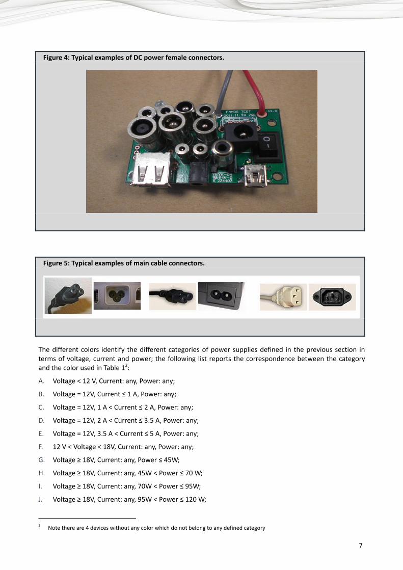
In the connector type column, the coaxial ones have been divided into classes (T1, T2, T3, T4, T5… T14) by following the internal and external sizes of the connectors. Some examples of DC power female connectors can be seen in Figure 4.

Remarks – It can be easily noticed that voltage, current and especially power values seem to tend to common ratings. This fact is conducive to a “de facto” standardization.

7

Figure 4: Typical examples of DC power female connectors.

Figure 5: Typical examples of main cable connectors.

The different colors identify the different categories of power supplies defined in the previous section in terms of voltage, current and power; the following list reports the correspondence between the category and the color used in Table 12:

A. Voltage < 12 V, Current: any, Power: any;

B. Voltage = 12V, Current ≤ 1 A, Power: any;

C. Voltage = 12V, 1 A < Current ≤ 2 A, Power: any;

D. Voltage = 12V, 2 A < Current ≤ 3.5 A, Power: any;

E. Voltage = 12V, 3.5 A < Current ≤ 5 A, Power: any;

F. 12 V < Voltage < 18V, Current: any, Power: any;

G. Voltage ≥ 18V, Current: any, Power ≤ 45W;

H. Voltage ≥ 18V, Current: any, 45W < Power ≤ 70 W;

I. Voltage ≥ 18V, Current: any, 70W < Power ≤ 95W;

J. Voltage ≥ 18V, Current: any, 95W < Power ≤ 120 W;

2 Note there are 4 devices without any color which do not belong to any defined category

8

Moreover, Figure 6 summarizes the numerical and percentage impact of the different categories on the total number of the equipment measured.

Figure 6: Numerical and percentage impact of the different defined categories with respect to the total number of measured devices.

A: < 12 V B: 12V, ≤ 1 A C: 12V, 1 A < I ≤ 2 A D: 12V, 2 A < I ≤ 3.5 A E: 12V, 3.5 A < I ≤ 5 A F: >12V ÷ 18V G: ≥ 18V, Power ≤ 45W; H: ≥ 18V, 45W ÷ 70 W; I: ≥ 18V, 70W ÷ 95W; J: ≥ 18V, 95W ÷ 120 W;

9

Table 1: Nameplate and measured mechanical features of the analyzed adapters

N.

Out

put v

olta

ge [V

]

Out

put c

urre

nt [A

]

Rate

d ou

tput

pow

er [W

]

Safe

ty c

lass

Ener

gy st

ar c

lass

Wei

ght w

ithou

t cab

le (g

)

Wei

ght w

ith c

able

(g)

Volu

me

(cm

³)

Conn

ecto

r’s ty

pe

Deta

chab

le m

ain

cabl

e (c

onne

ctor

)

mW

/cm

³

mW

/g

167 1.9 1.4 2.66 2 - 143 - 141 Proprietary NO 19 19 166 3 1 3 2 - 235 - 268 Proprietary NO 11 13 138 4 0.15 - 2 V 98 - 82 - NO - - 89 4.5 0.7 3.15 2 - 233 - 243 T4 NO 13 14 57 4.9 0.45 2.205 2 - 68 - 161 Proprietary NO 14 32 17 5 0.3 1.5 1 - 69 - 145 T3 NO 10 22

137 5 0.5 2.5 2 IV 141 - 286 Proprietary NO 9 18 8 5 1 5 2 - 110 - 118 T6 NO 42 45

82 5 1 5 2 - 65 - 165 T8 NO 30 77 97 5 1 5 2 IV 68 - 110 USB NO 45 74

159 5 1 5 2 - 65 - 142 T4 NO 35 77 183 5 1 5 2 IV 83 - 150 Proprietary NO 33 60 253 5 1 5 2 V 71 - 72 T9 NO 70 70 302 5 1 5 2 V 71 - 72 T9 NO 70 70 46 5 1.4 7 2 - 100 - 151 T8 NO 46 70 31 5 1.5 7.5 2 - 122 - 179 T8 NO 42 61

113 5 1.5 7.5 2 - 128 - 225 T8 NO 33 59 114 5 1.5 7.5 2 - 128 - 225 T8 NO 33 59 157 5 1.5 7.5 2 - 89 - 123 T4 NO 61 84 300 5 1.5 7.5 2 - 119 - 182 T8 NO 41 63 318 5 1.5 7.5 2 - 120 - 104 T8 NO 72 63 243 5 1.5 7.5 2 - 66 - 62 T4 NO 121 114 319 5 1.5 7.5 2 - 120 - 104 T8 NO 72 63

5 5 2 10 2 - 102 - 90 T8 NO 111 98 23 5 2 10 1 - 160 352 176 T8 C13-C14 57 63 58 5 2 10 2 - 96 - 172 T8 NO 58 104 64 5 2 10 2 IV-V 110 - 208 T8 NO 48 91 98 5 2 10 2 - 45 - 114 USB NO 88 222

108 5 2 10 1 - 159 - 189 T8 C13-C14 53 63 115 5 2 10 2 - 146 - 224 T9 NO 45 68 154 5 2 10 2 - 144 - 239 T9 NO 42 69 177 5 2 10 2 - 144 - 238 T9 NO 42 69 195 5 2 10 1 - 172 - 174 T10 C13-C14 57 58 260 5 2 10 2 V 54 - 88 USB NO 114 185 261 5 2 10 2 V 54 - 88 USB NO 114 185

10

N.

Out

put v

olta

ge [V

]

Out

put c

urre

nt [A

]

Rate

d ou

tput

pow

er [W

]

Safe

ty c

lass

Ener

gy st

ar c

lass

Wei

ght w

ithou

t cab

le (g

)

Wei

ght w

ith c

able

(g)

Volu

me

(cm

³)

Conn

ecto

r’s ty

pe

Deta

chab

le m

ain

cabl

e (c

onne

ctor

)

mW

/cm

³

mW

/g

359 5 2 10 2 IV 96 - 115 T8 NO 87 104 10 5 2.5 12.5 2 - 156 - 333 T8 NO 38 80 20 5 2.5 12.5 2 - 156 - 333 T8 NO 38 80

191 5 2.5 12.5 2 - 156 - 198 T10 NO 63 80 179 5 3 15 1 - 206 - 195 T8 C13-C14 77 73 94 5.2 0.45 2.34 2 - 79 - 172 Proprietary NO 14 30

155 5.2 0.45 2.34 2 - 79 - 158 Proprietary NO 15 30 200 5.5 2.2 12.1 2 - 150 - 94 T10 C7-C8 128 81 28 5.7 3 17.1 2 IV 223 - 189 T8 C7-C8 91 77 80 6 0.2 1.2 2 - 287 - 252 RJ NO 5 4 6 6 0.3 1.8 2 - 195 - 225 T3 NO 8 9

21 6 0.3 1.8 2 - 196 - 228 T3 NO 8 9 84 6 0.3 1.8 2 - 171 - 180 T3 NO 10 11

172 6 0.3 1.8 2 - 274 - 233 T4 NO 8 7 79 6 0.5 3 2 V 67 - 106 T8 NO 28 45

176 6 2.5 15 2 - 187 - 227 T8 NO 66 80 165 6.5 0.3 1.95 2 V 55 - 83 T10 NO 24 35

2 6.5 0.2-0.4 2.6 2 - 317 - 328 Proprietary NO 8 8 12 6.5 0.2-0.4 2.6 2 - 317 - 328 RJ NO 8 8 38 7.5 0.3 2.25 2 V 70 - 114 RJ NO 20 32 83 7.5 0.8 6 2 - 328 - 296 T3 NO 20 18

164 7.5 0.8 6 2 - 294 - 246 T3 NO 24 20 27 8 1 8 2 - 271 - 235 T8 NO 34 30

160 9 0.2 1.8 2 - 273 - 275 RJ NO 7 7 163 9 0.3 2.7 2 - 222 - 239 T8 NO 11 12 134 9 0.4 3.6 2 - 162 - 186 Male Coaxial NO 19 22 19 9 0.5 4.5 2 - 256 - 253 T8 NO 18 18 29 9 0.6 5.4 2 - 96 - 164 T9 NO 33 56 88 9 0.6 5.4 2 - 96 - 156 T9 NO 35 56 26 9 1 9 2 - 556 - 382 T8 NO 24 16 99 9 1 9 2 - 327 - 226 T9 NO 40 28

106 9 1 9 2 - 550 - 386 T8 NO 23 16 122 9 1 9 2 - 440 - 354 T8 NO 25 20 363 9 1 9 2 V 118 - 85 T8 NO 106 76 170 9 1.2 10.8 2 - 523 - 352 T9 NO 31 21 131 9 2 18 2 - 149 - 200 T8 NO 90 121 127 9.5 0.4 3.8 2 - 194 - 195 T9 NO 20 20

11

N.

Out

put v

olta

ge [V

]

Out

put c

urre

nt [A

]

Rate

d ou

tput

pow

er [W

]

Safe

ty c

lass

Ener

gy st

ar c

lass

Wei

ght w

ithou

t cab

le (g

)

Wei

ght w

ith c

able

(g)

Volu

me

(cm

³)

Conn

ecto

r’s ty

pe

Deta

chab

le m

ain

cabl

e (c

onne

ctor

)

mW

/cm

³

mW

/g

169 9.5 2.7 25.65 2 - 211 299 172 Proprietary C7-C8 149 122 205 9.5 3.78 36 2 - 162 267 78 T5 C7-C8 463 222 241 10.5 2.9 30 2 V 141 193 91 Proprietary C7-C8 328 213 22 12 0.2 2.4 2 - 187 - 215 T5 NO 11 13 25 12 0.3 3.6 2 - 246 - 263 T8 NO 14 15 76 12 0.33 3.96 2 - 58 - 81 T9 NO 49 68 93 12 0.4 4.8 2 - 290 - 272 T9 NO 18 17

174 12 0.4 4.8 2 - 91 - 81 Proprietary NO 59 53 77 12 0.5 6 2 - 300 - 238 T8 NO 25 20

258 12 0.5 6 2 V 71 - 137 T8 NO 44 85 259 12 0.5 6 2 V 71 - 137 T8 NO 44 85 362 12 0.5 6 2 V 76 - 118 T4 NO 51 79 95 12 0.6 7.2 2 - 313 - 257 RJ NO 28 23 55 12 0.8 9.6 2 - 96 - 153 T8 NO 63 100 59 12 0.8 9.6 2 - 76 - 191 T8 NO 50 126

324 12 0.8 9.6 2 - 88 - 83 T8 NO 116 109 18 12 0.83 9.96 2 - 167 - 330 T8 NO 30 60 54 12 0.83 9.96 2 - 328 - 256 T8 NO 39 30 4 12 1 12 1 - 167 - 180 T8 C13-C14 67 72

40 12 1 12 2 V 129 - 162 T6 NO 74 93 63 12 1 12 2 - 110 - 177 T8 NO 68 109 68 12 1 12 2 - 127 - 264 T8 NO 45 94 70 12 1 12 2 - 530 - 412 T8 NO 29 23 71 12 1 12 2 - - - 391 - NO 31 - 72 12 1 12 2 - 110 - 177 T8 NO 68 109

107 12 1 12 2 - 285 367 197 Proprietary C7-C8 61 42 116 12 1 12 1 - 215 236 202 T8 male C13-C14 59 56 117 12 1 12 1 - 210 236 197 T8 male C13-C14 61 57 143 12 1 12 2 - 127 - 264 T8 NO 45 94 146 12 1 12 2 - 127 - 264 T8 NO 45 94 152 12 1 12 2 - 127 - 264 T8 NO 45 94 181 12 1 12 2 V 110 - 151 T6 NO 79 109 208 12 1 12 2 V 110 - 151 T6 NO 79 109 254 12 1 12 2 V 125 - 286 T8 NO 42 96 255 12 1 12 2 V 125 - 286 T8 NO 42 96 256 12 1 12 2 V 119 - 284 T8 NO 42 101 257 12 1 12 2 V 119 - 284 T8 NO 42 101

12

N.

Out

put v

olta

ge [V

]

Out

put c

urre

nt [A

]

Rate

d ou

tput

pow

er [W

]

Safe

ty c

lass

Ener

gy st

ar c

lass

Wei

ght w

ithou

t cab

le (g

)

Wei

ght w

ith c

able

(g)

Volu

me

(cm

³)

Conn

ecto

r’s ty

pe

Deta

chab

le m

ain

cabl

e (c

onne

ctor

)

mW

/cm

³

mW

/g

309 12 1 12 2 V 100 - 112 T8 NO 107 120 322 12 1 12 2 - 129 - 123 T8 NO 97 93 65 12 - 12.5 2 - 283 - 320 T9 NO 39 44 44 12 1.2 14.4 2 - 84 - 188 T8 NO 77 171 67 12 1.2 14.4 2 - 559 - 398 T8 NO 36 26

323 12 1.2 14.4 2 - 96 - 86 T8 NO 167 150 16 12 1.25 15 2 - 124 - 207 T8 NO 73 121 45 12 1.25 15 1 V 128 - 122 T9 C13-C14 122 117 60 12 1.25 15 2 V 122 - 233 T8 NO 64 123 73 12 1.25 15 1 V 143 - 169 T8 C13-C14 89 105 74 12 1.25 15 2 V 172 - 203 T9 NO 74 87

110 12 1.25 15 1 - 198 - 146 T9 NO 103 76 197 12 1.25 15 2 - 236 - 287 T8 NO 52 64 198 12 1.25 15 2 - 123 - 202 T8 NO 74 122 61 12 1.4 16.8 2 - - - 190 T9 NO 89 - 75 12 1.4 16.8 2 V 104 - 191 T9 NO 88 162 7 12 1.5 18 2 - 133 - 200 T8 NO 90 135

43 12 1.5 18 2 - 145 - 254 T9 NO 71 124 52 12 1.5 18 2 - - - 238 - NO 76 - 56 12 1.5 18 1 - 120 - 126 T8 C13-C14 143 150 69 12 1.5 18 2 - 148 - 212 T8 NO 85 122 85 12 1.5 18 2 - 153 - 316 T3 NO 57 118

103 12 1.5 18 2 V 133 - 200 T8 NO 90 135 105 12 1.5 18 2 V 146 - 277 T8 NO 65 123 111 12 1.5 18 2 - 147 - 211 T8 NO 85 122 119 12 1.5 18 2 - 147 - 211 T8 NO 85 122 120 12 1.5 18 1 - 189 - 172 T8 C13-C14 105 95 126 12 1.5 18 2 - 140 - 241 T9 NO 75 129 149 12 1.5 18 2 - 189 - 170 T8 C13-C14 106 95 150 12 1.5 18 2 - 147 - 211 T8 NO 85 122 151 12 1.5 18 1 - 189 - 169 T8 C13-C14 107 95 202 12 1.5 18 2 - 154 - 247 T8 NO 73 117 242 12 1.5 18 2 V 127 - 109 T2 NO 166 142 201 12 1.6 19.2 2 - 193 - 276 T8 NO 70 99 203 12 1.7 20.4 2 - 166 - 295 T10 NO 69 123 13 12 2 24 2 - 132 - 97 T9 C7-C8 247 182 36 12 2 24 2 V 170 - 230 T12 NO 104 141

13

N.

Out

put v

olta

ge [V

]

Out

put c

urre

nt [A

]

Rate

d ou

tput

pow

er [W

]

Safe

ty c

lass

Ener

gy st

ar c

lass

Wei

ght w

ithou

t cab

le (g

)

Wei

ght w

ith c

able

(g)

Volu

me

(cm

³)

Conn

ecto

r’s ty

pe

Deta

chab

le m

ain

cabl

e (c

onne

ctor

)

mW

/cm

³

mW

/g

39 12 2 24 2 V 142 - 181 T6 NO 132 169 47 12 2 24 2 V 220 308 144 T9 C7-C8 166 109

102 12 2 24 2 - 185 - 323 T8 NO 74 130 104 12 2 24 2 - 150 - 252 T5 NO 95 160 112 12 2 24 1 - 156 - 254 T8 NO 94 154 129 12 2 24 2 - 131 - 240 T8 NO 100 183 145 12 2 24 1 - 207 - 167 T10 C13-C14 144 116 156 12 2 24 2 - 119 - 207 T8 NO 116 202 171 12 2 24 2 IV 158 - 220 T8 NO 109 152 173 12 2 24 2 V 145 - 287 T9 NO 84 166 180 12 2 24 2 V 141 - 182 T6 NO 132 170 184 12 2 24 2 V 189 - 333 T4 NO 72 127 189 12 2 24 2 IV 160 - 286 T8 NO 84 150 199 12 2 24 2 V 142 - 305 T9 NO 79 169 207 12 2 24 2 V 145 - 287 T9 NO 84 166 251 12 2 24 2 V 155 - 276 T8 NO 87 155 252 12 2 24 2 V 155 - 276 T8 NO 87 155 321 12 2 24 2 - 179 - 131 T8 NO 183 134 317 12 2.1 25.2 2 - 157 - 156 T8 NO 162 161 41 12 2.5 30 2 - 248 - 205 T9 C7-C8 147 121 42 12 2.5 30 2 IV 163 240 134 T8 C7-C8 225 184 48 12 2.5 30 2 IV 223 - 390 T9 NO 77 135

187 12 2.5 30 2 IV 200 298 166 T3 C7-C8 181 150 148 12 3 36 2 - 290 377 222 T8 C7-C8 162 124 178 12 3 36 2 - 214 - 133 T9 C7-C8 270 168 185 12 3 36 2 V 158 212 79 T5 C7-C8 454 228 206 12 3 36 2 - 162 267 78 T5 C7-C8 463 222 357 12 3 36 2 IV 151 200 76 T5 C7-C8 476 238 15 12 3.3 39.6 1 - 312 - 266 T8 C13-C14 149 127

121 12 3.3 39.6 1 - 309 - 257 T8 C13-C14 154 128 147 12 3.3 39.6 1 - 309 - 257 T8 C13-C14 154 128 141 12 3.7 44.4 2 - 338 440 372 Proprietary NO 119 131 142 12 3.7 44.4 2 - 338 440 372 Proprietary NO 119 131 24 12 3.75 45 1 - 309 - 291 T9 C13-C14 155 146 87 12 4.2 50 1 - 325 - 330 T8 NO 152 154

123 12 4.16 50 1 - 253 - 219 T9 C13-C14 229 198 140 12 14.2 170.4 2 - 840 979 1246 Proprietary C17-C18 137 203

14

N.

Out

put v

olta

ge [V

]

Out

put c

urre

nt [A

]

Rate

d ou

tput

pow

er [W

]

Safe

ty c

lass

Ener

gy st

ar c

lass

Wei

ght w

ithou

t cab

le (g

)

Wei

ght w

ith c

able

(g)

Volu

me

(cm

³)

Conn

ecto

r’s ty

pe

Deta

chab

le m

ain

cabl

e (c

onne

ctor

)

mW

/cm

³

mW

/g

153 13 0.625 8.1 2 - 543 - 445 T6 NO 18 15 96 15 - 5.4 2 V 62 - 78 Proprietary NO 69 87

301 15 0.5 7.5 2 - 83 - 88 T8 NO 86 90 11 15 0.8 12 2 - 132 - 126 T8 NO 95 91 37 15 0.8 12 2 V 100 - 153 T8 NO 79 120 62 15 0.8 12 2 - 138 - 227 T8 NO 53 87 9 15 1 15 2 - 453 - 387 T8 NO 39 33

49 15 2 18 2 IV 124 - 219 T8 NO 82 145 51 15 1.2 18 2 - 149 - 277 T8 NO 65 121 78 15 1.2 18 2 - 149 - 277 T8 NO 65 121 53 15 2 30 2 - 195 292 168 T8 C7-C8 179 154

109 15 2 30 2 - 195 - 168 T8 C7-C8 179 154 358 15 5 75 2 V 339 404 312 T12 C7-C8 240 221

3 16 3.36 53.76 2 - 254 - 157 T13 C7-C8 342 212 158 16 4.5 72 1 - 310 - 214 T9 C5-C6 337 232 168 18.5 2.7 50 1 - 258 461 138 T5 C5-C6 361 194 315 18.5 2.7 50 1 - 200 308 105 T5 C5-C6 477 250 188 18.5 3.5 64.75 1 IV 233 388 139 T14 C5-C6 466 278 250 18.5 3.5 64.75 1 IV 238 - 144 T6 C5-C6 451 272 306 18.5 3.5 65 1 IV 234 - 143 T5 C5-C6 455 278 308 18.5 3.5 65 1 V 253 401 145 T14 C5-C6 449 257 244 18.5 4.9 90 1 - 258 - 232 T5 C5-C6 388 349 245 18.5 4.9 90 1 - 267 - 242 T14 C5-C6 372 337 247 18.5 4.9 90 1 - 259 - 246 T5 C5-C6 366 347 192 18.5 4.9 90.65 1 - 320 463 231 T5 C5-C6 393 283 118 18.5 6.5 120 1 - 639 - 396 T9 C5-C6 303 188 124 18.5 6.5 120 1 - 659 812 399 T9 C5-C6 301 182 209 18.5 6.5 120 1 V 609 763 354 T14 C5-C6 339 197 210 18.5 6.5 120 1 V 609 763 354 T14 C5-C6 339 197 211 18.5 6.5 120 1 V 630 786 357 T14 C5-C6 336 190 217 18.5 6.5 120 1 V 630 782 351 T14 C5-C6 342 190 218 18.5 6.5 120 1 V 609 763 354 T14 C5-C6 339 197 360 18.5 6.5 120 1 V 612 745 361 T14 C5-C6 333 196 361 18.5 6.5 120 1 NA 651 761 412 T9 C5-C6 291 184 246 18.5 - - 1 - 261 - 244 T5 C5-C6 - - 35 19 1 19 2 V 105 2 82 - C7-C8 232 181 33 19 1.5 28.5 - OK - - - - C5-C6 - -

15

N.

Out

put v

olta

ge [V

]

Out

put c

urre

nt [A

]

Rate

d ou

tput

pow

er [W

]

Safe

ty c

lass

Ener

gy st

ar c

lass

Wei

ght w

ithou

t cab

le (g

)

Wei

ght w

ith c

able

(g)

Volu

me

(cm

³)

Conn

ecto

r’s ty

pe

Deta

chab

le m

ain

cabl

e (c

onne

ctor

)

mW

/cm

³

mW

/g

186 19 1.58 30 1 V 145 300 84 T5 C5-C6 355 207 238 19 1.58 30 2 V 152 - 84 T1 NO 355 197 240 19 1.58 30 1 V 170 360 104 T10 C5-C6 288 176 316 19 1.58 30 1 V 129 265 84 T5 C5-C6 357 233 346 19 1.58 30 1 V 142 274 84 T5 C5-C6 357 211 347 19 1.58 30 1 V 142 274 84 T5 C5-C6 357 211 348 19 1.58 30 1 V 171 306 100 T5 C5-C6 302 175 349 19 1.58 30 1 V 171 306 100 T5 C5-C6 302 175 350 19 1.58 30 1 V 171 306 100 T5 C5-C6 302 175 351 19 1.58 30 1 V 171 306 100 T5 C5-C6 302 175 352 19 1.58 30 1 V 151 282 100 T5 C5-C6 302 199 353 19 1.58 30 1 IV 163 293 110 T7 C5-C6 272 184 86 19 2.15 40 2 V 209 - 277 T7 NO 144 191

233 19 2.15 40 2 V 209 - 120 T8 NO 332 191 237 19 2.15 40 2 V 193 - 123 T8 NO 326 207 313 19 2.1 40 2 V 152 206 86 T1 C7-C8 467 263 314 19 2.1 40 2 V 152 206 86 T1 C7-C8 467 263 194 19 3.16 60 1 - 291 - 203 T7 C5-C6 295 206 132 19 3.42 65 1 V 238 390 141 T9 C5-C6 462 273 232 19 3.42 65 1 V 243 398 156 T8 C5-C6 417 267 234 19 3.42 65 1 V 220 376 124 T8 C5-C6 526 295 303 19 3.42 65 1 V 246 400 152 T7 C5-C6 428 264 311 19 3.42 65 1 IV 234 342 145 T9 C5-C6 447 278 320 19 3.42 65 1 V 209 364 147 T9 C5-C6 443 311 325 19 3.42 65 1 V 213 364 147 T9 C5-C6 443 305 326 19 3.42 65 1 V 213 364 147 T9 C5-C6 443 305 327 19 3.42 65 1 V 213 364 147 T9 C5-C6 443 305 328 19 3.42 65 1 V 213 364 147 T9 C5-C6 443 305 329 19 3.42 65 1 V 213 364 147 T9 C5-C6 443 305 330 19 3.42 65 1 V 213 364 147 T9 C5-C6 443 305 331 19 3.42 65 1 V 213 364 147 T9 C5-C6 443 305 332 19 3.42 65 1 V 213 364 147 T9 C5-C6 443 305 333 19 3.42 65 1 V 213 364 147 T9 C5-C6 443 305 334 19 3.42 65 1 V 213 364 147 T9 C5-C6 443 305 335 19 3.42 65 1 V 213 364 147 T9 C5-C6 443 305 354 19 3.42 65 1 V 213 364 147 T9 C5-C6 443 305 356 19 3.42 65 1 V 247 377 148 T9 C5-C6 440 263

16

N.

Out

put v

olta

ge [V

]

Out

put c

urre

nt [A

]

Rate

d ou

tput

pow

er [W

]

Safe

ty c

lass

Ener

gy st

ar c

lass

Wei

ght w

ithou

t cab

le (g

)

Wei

ght w

ith c

able

(g)

Volu

me

(cm

³)

Conn

ecto

r’s ty

pe

Deta

chab

le m

ain

cabl

e (c

onne

ctor

)

mW

/cm

³

mW

/g

125 19 4.74 90 1 - 354 - 235 T11 C5-C6 384 254 175 19 4.74 90 1 - 358 509 190 T5 C5-C6 473 251 182 19 4.74 90 1 V 327 469 192 T5 C5-C6 469 275 190 19 4.74 90 1 - 261 401 241 T14 C5-C6 373 345 193 19 4.74 90 1 IV 347 484 186 T5 C5-C6 484 259 204 19 4.74 90 1 V 352 535 187 T14 C5-C6 480 256 212 19 4.7 90 1 V 355 510 188 T14 C5-C6 478 254 213 19 4.74 90 1 V 360 460 196 T14 C5-C6 460 250 214 19 4.74 90 1 V 351 510 194 T14 C5-C6 463 256 215 19 4.7 90 1 V 353 410 357 T14 C5-C6 252 255 216 19 4.74 90 1 V 343 436 194 T14 C5-C6 463 262 219 19 4.7 90 1 V 360 515 188 T14 C5-C6 478 250 220 19 4.7 90 1 V 355 510 188 T14 C5-C6 478 254 221 19 4.74 90 1 V 341 503 194 T14 C5-C6 463 264 222 19 4.74 90 1 V 364 500 243 T8 C5-C6 370 247 223 19 4.74 90 1 V 364 500 243 T8 C5-C6 370 247 224 19 4.74 90 1 V 386 545 229 T8 C5-C6 394 233 225 19 4.74 90 1 V 390 545 229 T8 C5-C6 394 231 226 19 4.74 90 1 V 345 495 195 T8 C5-C6 461 261 227 19 4.74 90 1 V 342 472 194 T8 C5-C6 463 263 228 19 4.74 90 1 V 342 472 194 T8 C5-C6 463 263 229 19 4.74 90 1 V 364 500 243 T8 C5-C6 370 247 230 19 4.74 90 1 V 345 496 195 T8 C5-C6 461 261 231 19 4.74 90 1 V 364 517 243 T8 C5-C6 370 247 236 19 4.74 90 1 V 365 519 243 T8 C5-C6 370 247 239 19 4.74 90 1 V 363 500 247 T8 C5-C6 365 248 248 19 4.7 90 1 - 348 - 188 T5 C5-C6 479 259 249 19 4.7 90 1 - 349 - 186 T5 C5-C6 485 258 304 19 4.74 90 2 V 300 365 228 T14 C7-C8 395 300 305 19 4.74 90 1 - 341 - 185 T5 C5-C6 488 264 307 19 4.74 90 1 - 261 440 243 T14 C5-C6 371 345 312 19 4.74 90 1 IV 342 520 193 T14 C5-C6 466 263 235 19 6.32 120 1 V 590 728 351 T8 C5-C6 342 203 128 20 1 20 2 IV 143 - 293 T8 NO 68 140 100 20 2.5 50 1 IV 354 541 252 Proprietary C5-C6 198 141 310 20 3.25 65 2 V 230 287 126 T13 C7-C8 516 283 336 20 4.5 90 2 IV 369 449 269 T9 C7-C8 335 244

17

N.

Out

put v

olta

ge [V

]

Out

put c

urre

nt [A

]

Rate

d ou

tput

pow

er [W

]

Safe

ty c

lass

Ener

gy st

ar c

lass

Wei

ght w

ithou

t cab

le (g

)

Wei

ght w

ith c

able

(g)

Volu

me

(cm

³)

Conn

ecto

r’s ty

pe

Deta

chab

le m

ain

cabl

e (c

onne

ctor

)

mW

/cm

³

mW

/g

337 20 4.5 90 2 IV 369 449 269 T9 C7-C8 335 244 338 20 4.5 90 2 IV 369 449 269 T9 C7-C8 335 244 339 20 4.5 90 2 IV 369 449 269 T9 C7-C8 335 244 340 20 4.5 90 2 IV 369 449 269 T9 C7-C8 335 244 341 20 4.5 90 2 IV 369 449 269 T9 C7-C8 335 244 342 20 4.5 90 2 IV 369 449 269 T9 C7-C8 335 244 343 20 4.5 90 2 IV 369 449 269 T9 C7-C8 335 244 344 20 4.5 90 2 IV 369 449 269 T9 C7-C8 335 244 345 20 4.5 90 2 IV 369 449 269 T9 C7-C8 335 244 355 20 4.5 90 2 IV 369 449 269 T9 C7-C8 335 244 81 24 6 120 1 - 557 700 427 T5 C13-C14 281 215

135 32 0.7 22.4 2 IV 209 295 196 Proprietary C7-C8 114 107 1 - - - 2 - 115 - 179 T8 NO - -

For each model, the rated voltage, current and power on the DC side are reported, together with the safety and Energy Star class and other features such as the weight of the power supply (with and without cables), volume, information about the low voltage connector, the manufacturing country and information on the presence of a detachable main cable or a main connector integrated with the power supply itself. About 90% of the adapters analyzed were made in China.

Figure 7 demonstrates the percentage of the connectors belonging to each different category. It can be noticed that the majority of the connectors are barrel type. The five most used connectors represent 86% of the total. We recall that all the connectors except those in the category “other” are barrel ones and the classification have been made by using the internal and external size measurements. The “other” category is a mix of many different connectors such as USB, RJ and proprietary.

18

Figure 7: Used connector percentage versus connector types.

Taking the T8 category (the largest one) as an example, Figure 8 clearly highlights that the same type of connector is used for power supplies with a different output voltage, from 5V to 20V.

Figure 8: Percentage of connectors belonging to category T8 versus the nameplate output voltage of their power supplies.

19

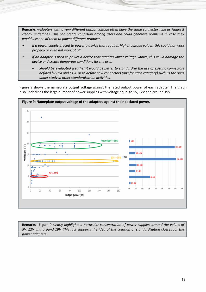
Remarks –Adapters with a very different output voltage often have the same connector type as Figure 8 clearly underlines. This can create confusion among users and could generate problems in case they would use one of them to power different products.

• If a power supply is used to power a device that requires higher voltage values, this could not work properly or even not work at all.

• If an adapter is used to power a device that requires lower voltage values, this could damage the device and create dangerous conditions for the user.

– Should be evaluated weather it would be better to standardize the use of existing connectors defined by HGI and ETSI, or to define new connectors (one for each category) such us the ones under study in other standardization activities.

Figure 9 shows the nameplate output voltage against the rated output power of each adapter. The graph also underlines the large number of power supplies with voltage equal to 5V, 12V and around 19V.

Figure 9: Nameplate output voltage of the adapters against their declared power.

Remarks –Figure 9 clearly highlights a particular concentration of power supplies around the values of 5V, 12V and around 19V. This fact supports the idea of the creation of standardization classes for the power adapters.

20

4. Mechanical features

4.1 Weight

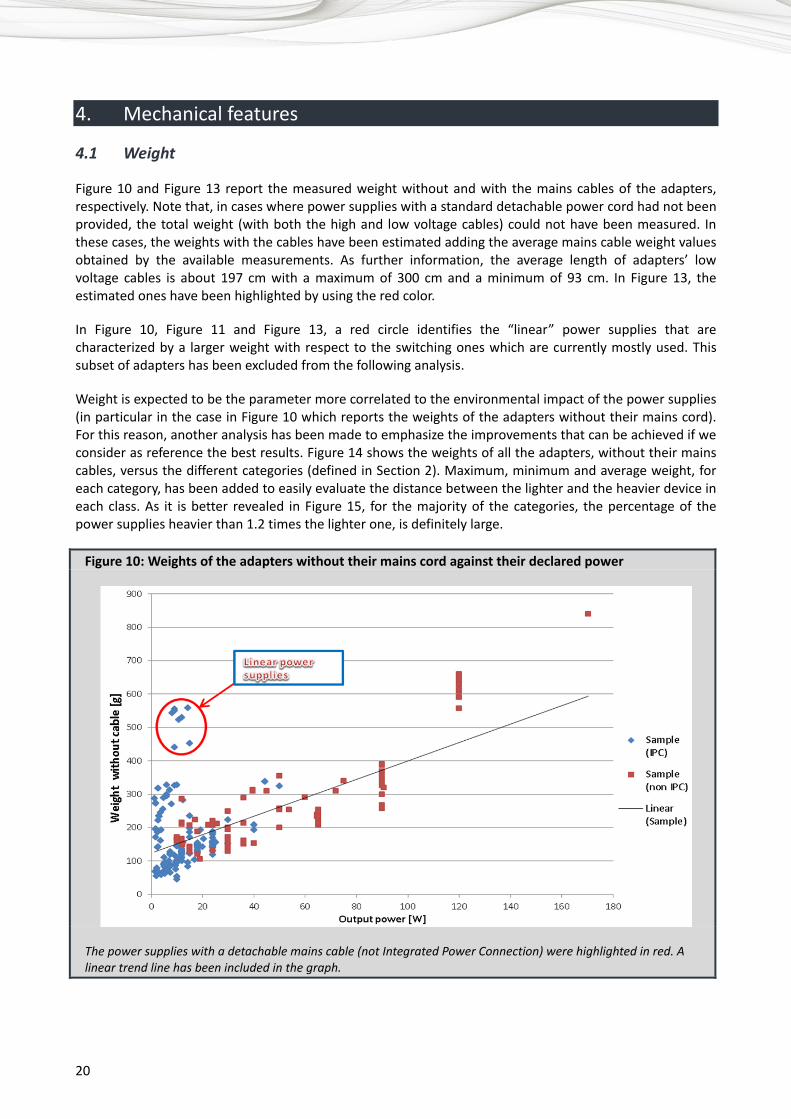
Figure 10 and Figure 13 report the measured weight without and with the mains cables of the adapters, respectively. Note that, in cases where power supplies with a standard detachable power cord had not been provided, the total weight (with both the high and low voltage cables) could not have been measured. In these cases, the weights with the cables have been estimated adding the average mains cable weight values obtained by the available measurements. As further information, the average length of adapters’ low voltage cables is about 197 cm with a maximum of 300 cm and a minimum of 93 cm. In Figure 13, the estimated ones have been highlighted by using the red color.

In Figure 10, Figure 11 and Figure 13, a red circle identifies the “linear” power supplies that are characterized by a larger weight with respect to the switching ones which are currently mostly used. This subset of adapters has been excluded from the following analysis.

Weight is expected to be the parameter more correlated to the environmental impact of the power supplies (in particular in the case in Figure 10 which reports the weights of the adapters without their mains cord). For this reason, another analysis has been made to emphasize the improvements that can be achieved if we consider as reference the best results. Figure 14 shows the weights of all the adapters, without their mains cables, versus the different categories (defined in Section 2). Maximum, minimum and average weight, for each category, has been added to easily evaluate the distance between the lighter and the heavier device in each class. As it is better revealed in Figure 15, for the majority of the categories, the percentage of the power supplies heavier than 1.2 times the lighter one, is definitely large.

Figure 10: Weights of the adapters without their mains cord against their declared power

The power supplies with a detachable mains cable (not Integrated Power Connection) were highlighted in red. A linear trend line has been included in the graph.

21

Figure 11: Weights of the adapters without their mains cord against their declared power, limited to the lower power category (≤ 40W).

The power supplies with a detachable cable (not Integrated Power Connection) were highlighted in red. A linear trend line has been included in the graph.

Figure 12: Weights of the adapters without their mains cord against their declared power, limited to the “higher” power category (>40W).

The power supplies with a detachable cable (not Integrated Power Connection) were highlighted in red. A linear trend line has been included in the graph.

22

Figure 13: Weights of the adapters with their mains and low voltage cable against their declared power. A linear trend line has been included in the graph.

Remarks – Figure 10 through Figure 13 show a high dispersion on weights of adapters having the same ratings. In particular for the lower power equipment (<40 to 50 W), Figure 11 shows substantial independence between weight and power, while the higher power equipment (laptop power supplies reported in Figure 12) look more aligned among themselves and they show a sort of linear dependence between power and weight.

As weight can be directly linked to the environmental impact, it would be advisable to urge manufacturers to take care of this issue and optimize their products aligning to what others already achieved.

A: < 12 V B: 12V, ≤ 1 A C: 12V, 1 A < I ≤ 2 A D: 12V, 2 A < I ≤ 3.5 A E: 12V, 3.5 A < I ≤ 5 A F: >12V ÷ 18V G: ≥ 18V, Power ≤ 45W; H: ≥ 18V, 45W ÷ 70 W; I: ≥ 18V, 70W ÷ 95W; J: ≥ 18V, 95W ÷ 120 W;

23

Figure 14: Weights of the adapters without their mains cord, divided by following the defined categories. For each category, maximum, minimum and average weights have been highlighted.

Figure 15: Percentage of power supplies that weigh more than the best in class plus the 20% of its weight, for each category.

The above analysis (Figure 11 and Figure 14) shows that the mean weight of equipment rated up to 40W is substantially stable and independent from the actual rated power and is rather higher than that of the lightest EPSs in those classes. Above 40W (Figure 12 and Figure 14), there is an evident linear relationship between rated power and weight while the spread is reduced.

A: < 12 V B: 12V, ≤ 1 A C: 12V, 1 A < I ≤ 2 A D: 12V, 2 A < I ≤ 3.5 A E: 12V, 3.5 A < I ≤ 5 A F: >12V ÷ 18V G: ≥ 18V, Power ≤ 45W; H: ≥ 18V, 45W ÷ 70 W; I: ≥ 18V, 70W ÷ 95W; J: ≥ 18V, 95W ÷ 120 W;

24

Remarks –Figure 14 and Figure 15 clearly show the huge difference between the best and the worst adapter, in terms of weight, for each category. For most of the categories, the percentage of power supplies that weigh more than the best plus the 20% is really large. This demonstrates that a lot can still be done to minimize the environmental impact of the power supplies.

4.2 Volume

Similar to the previous graphs, Figure 16, Figure 17 and Figure 18 show the volumes measured for the set of analyzed devices according to their rated output power: Figure 16 for the total number of devices, Figure 17 for the “lower” power ones (≤40W), and Figure 18 for the “higher” power supplies.

The obtained results outline how the collected volume is almost not correlated with the adapter power for the lower power devices (the trend line is almost flat and there is a wide dispersion of the values) and that the correlation is very limited also for the higher power ones. Note that, in some cases, the measured devices with output power between 50 and 100 W appear to have smaller form-factors than the ones rated at 1-20 W.

Figure 16: Volumes of the adapters against their declared power. A linear trend line has been included in the graph.

25

Figure 17: Volumes of the adapters against their declared power, limited to the lower power category (≤ 40 W). A linear trend line has been included in the graph.

Figure 1: Volumes measured from the adapters without their cord against their declared power, limited to the “higher” power category (>40 W). A linear trend line has been included in the graph.

26

4.3 Power density

Figure 19 and Figure 20 report the power density (with respect to volume and weight, respectively) versus the output power. Though there is a wide dispersion of the values, some correlation can be found showing increase of mass and volume density with power increase.

Figure 19: Power density with respect to the weight (without cable), versus output power.

Figure 20: Power density with respect to the volume, versus output power.

27

4.4 Estimation on use of resources and e-waste

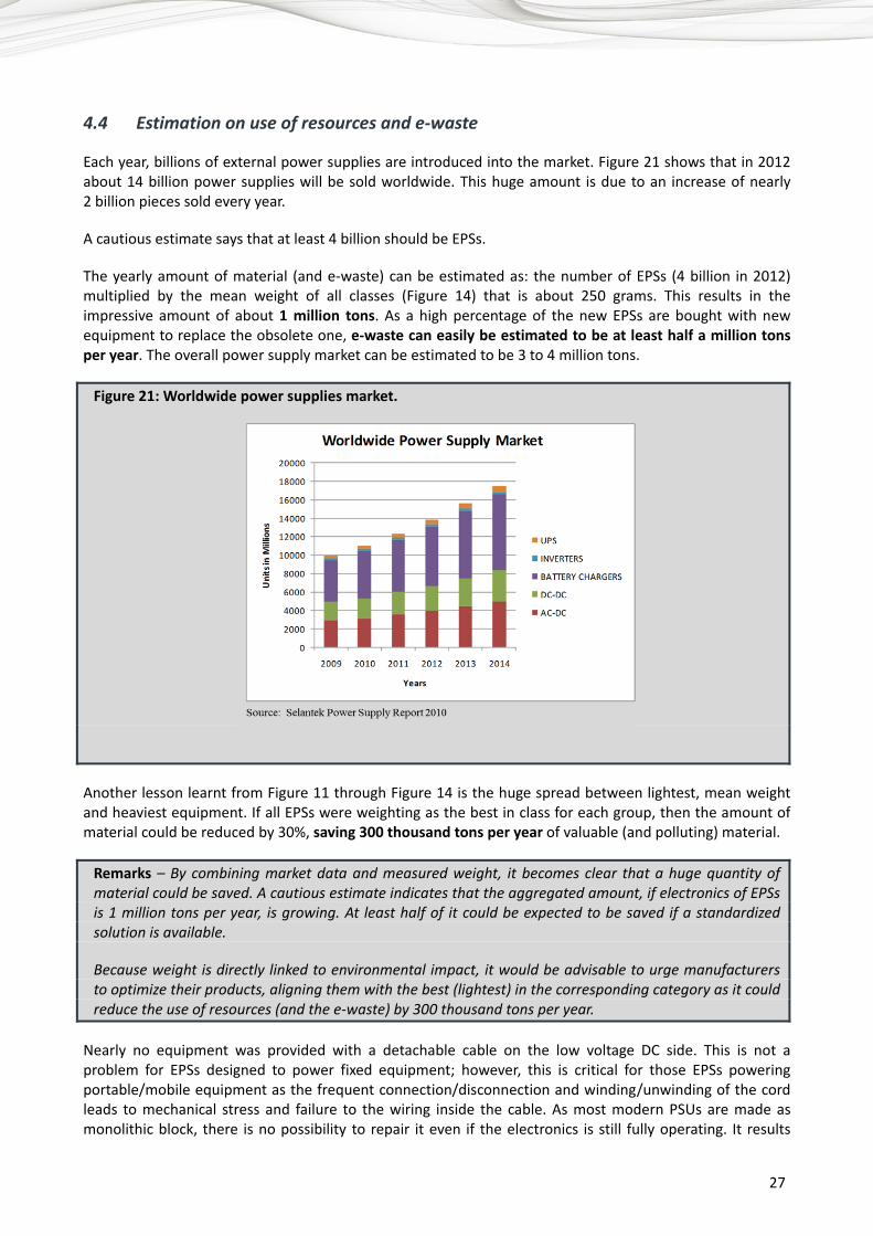
Each year, billions of external power supplies are introduced into the market. Figure 21 shows that in 2012 about 14 billion power supplies will be sold worldwide. This huge amount is due to an increase of nearly 2 billion pieces sold every year.

A cautious estimate says that at least 4 billion should be EPSs.

The yearly amount of material (and e-waste) can be estimated as: the number of EPSs (4 billion in 2012) multiplied by the mean weight of all classes (Figure 14) that is about 250 grams. This results in the impressive amount of about 1 million tons. As a high percentage of the new EPSs are bought with new equipment to replace the obsolete one, e-waste can easily be estimated to be at least half a million tons per year. The overall power supply market can be estimated to be 3 to 4 million tons.

Figure 21: Worldwide power supplies market.

Another lesson learnt from Figure 11 through Figure 14 is the huge spread between lightest, mean weight and heaviest equipment. If all EPSs were weighting as the best in class for each group, then the amount of material could be reduced by 30%, saving 300 thousand tons per year of valuable (and polluting) material.

Remarks – By combining market data and measured weight, it becomes clear that a huge quantity of material could be saved. A cautious estimate indicates that the aggregated amount, if electronics of EPSs is 1 million tons per year, is growing. At least half of it could be expected to be saved if a standardized solution is available.

Because weight is directly linked to environmental impact, it would be advisable to urge manufacturers to optimize their products, aligning them with the best (lightest) in the corresponding category as it could reduce the use of resources (and the e-waste) by 300 thousand tons per year.

Nearly no equipment was provided with a detachable cable on the low voltage DC side. This is not a problem for EPSs designed to power fixed equipment; however, this is critical for those EPSs powering portable/mobile equipment as the frequent connection/disconnection and winding/unwinding of the cord leads to mechanical stress and failure to the wiring inside the cable. As most modern PSUs are made as monolithic block, there is no possibility to repair it even if the electronics is still fully operating. It results

28

again into a high volume of unnecessary e-waste. This is a particular problem as Laptop PSUs are bulky and contain heavy electronics, and can weigh between 300 to 400 and sometimes even 600 grams each, while the DC cable alone weighs around 100 g. A Telecom Italy contribution to the January 2012 rapporteurs meeting of ITU-T SG5 WP3 has shown that in 9 out of 10 laptop EPSs reported as broken, the fault was located in the DC cable while the electronics was still fully operational.

5. Electrical features

5.1 Efficiency measurements

Figure 22 reports the energy-efficiency characteristic curves of the analyzed adapters. The energy efficiency curve is defined in each point as the ratio between the power provided at the DC side and the active power absorbed by the power supplies at the AC side. The tests were performed for each device up to its declared maximum current with steps of 50 mA or 100 mA as described above.

Most of the energy-efficiency curves have quite similar shapes: they rapidly increase and then flatten around a certain value, which represents the maximum efficiency level achievable by the adapter. Some of them are characterized by irregular slopes in the efficiency curves, and this behavior probably depends on internal circuitry design aiming at optimizing also the no-load behavior or the power factor at higher load.

Despite the similarity on the shapes of such curves, Figure 22 clearly shows that analyzed devices have highly heterogeneous values of maximum energy efficiency, and different paces to achieve these values.

Figure 22: Energy efficiency curves with variable loads for all the analyzed adapters. Each device has been tested up to its declared maximum value of DC current.

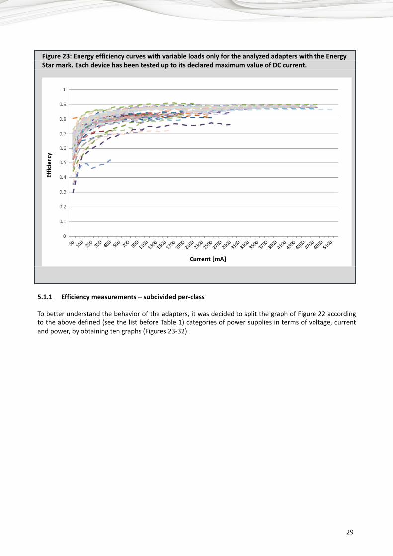
Figure 23 shows the efficiency curves only for the adapters with the Energy Star mark on their labels.

29

Figure 23: Energy efficiency curves with variable loads only for the analyzed adapters with the Energy Star mark. Each device has been tested up to its declared maximum value of DC current.

5.1.1 Efficiency measurements – subdivided per-class

To better understand the behavior of the adapters, it was decided to split the graph of Figure 22 according to the above defined (see the list before Table 1) categories of power supplies in terms of voltage, current and power, by obtaining ten graphs (Figures 23-32).

30

Figure 24: Energy efficiency curves with variable loads for the analyzed adapters. Each device has been tested up to its declared maximum value of DC current (Category A).

Voltage < 12 V, Current: any, Power: any;

Figure 25: Energy efficiency curves with variable loads for the analyzed adapters. Each device has been tested up to its declared maximum value of DC current (Category B).

Voltage = 12V, Current ≤ 1 A, Power: any;

31

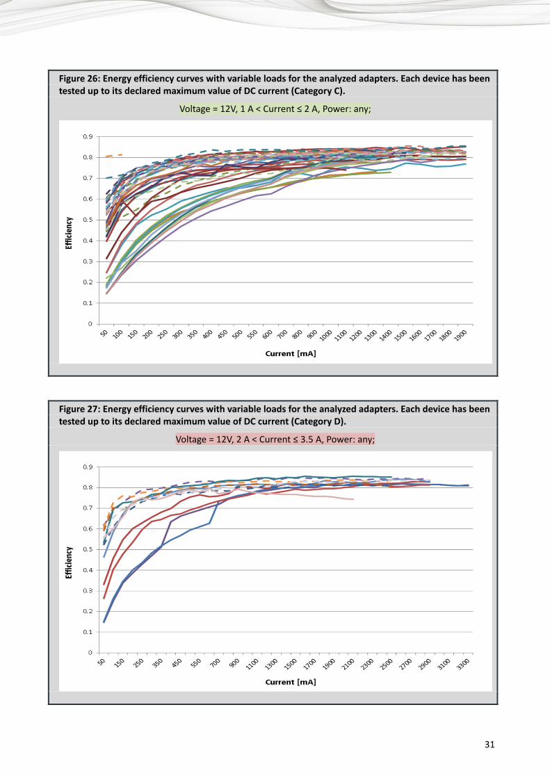
Figure 26: Energy efficiency curves with variable loads for the analyzed adapters. Each device has been tested up to its declared maximum value of DC current (Category C).

Voltage = 12V, 1 A < Current ≤ 2 A, Power: any;

Figure 27: Energy efficiency curves with variable loads for the analyzed adapters. Each device has been tested up to its declared maximum value of DC current (Category D).

Voltage = 12V, 2 A < Current ≤ 3.5 A, Power: any;

32

Figure 28: Energy efficiency curves with variable loads for the analyzed adapters. Each device has been tested up to its declared maximum value of DC current (Category E).

Voltage = 12V, 3.5 A < Current ≤ 5 A, Power: any;

Figure 29: Energy efficiency curves with variable loads for the analyzed adapters. Each device has been tested up to its declared maximum value of DC current (Category F).

12 V < Voltage < 18V, Current: any, Power: any;

33

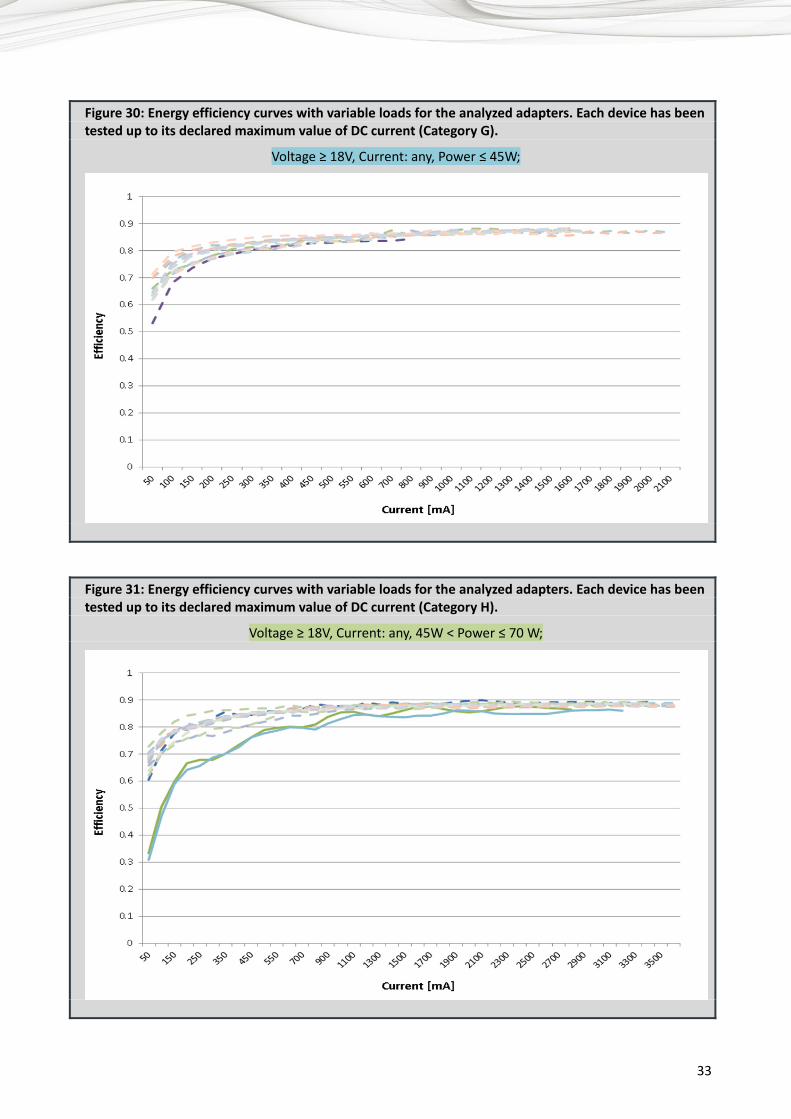
Figure 30: Energy efficiency curves with variable loads for the analyzed adapters. Each device has been tested up to its declared maximum value of DC current (Category G).

Voltage ≥ 18V, Current: any, Power ≤ 45W;

Figure 31: Energy efficiency curves with variable loads for the analyzed adapters. Each device has been tested up to its declared maximum value of DC current (Category H).

Voltage ≥ 18V, Current: any, 45W < Power ≤ 70 W;

34

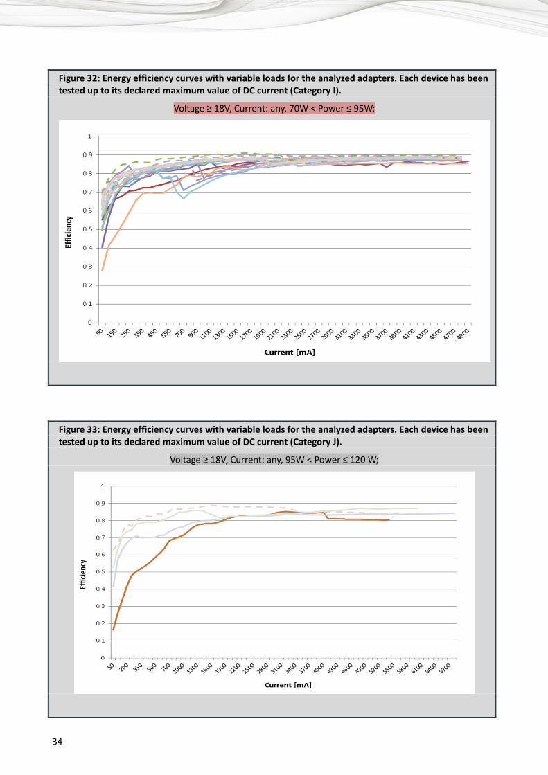
Figure 32: Energy efficiency curves with variable loads for the analyzed adapters. Each device has been tested up to its declared maximum value of DC current (Category I).

Voltage ≥ 18V, Current: any, 70W < Power ≤ 95W;

Figure 33: Energy efficiency curves with variable loads for the analyzed adapters. Each device has been tested up to its declared maximum value of DC current (Category J).

Voltage ≥ 18V, Current: any, 95W < Power ≤ 120 W;

35

Remarks – Graphs 22-33 show a high dispersion on the adapter efficiencies both in general (see graph Figure 22) and inside the same class. This aspect suggests an important opportunity of improving the efficiency characteristics of these devices independently from their power capacity.

In Figure 34, the efficiency result averages for each category are summarized and compared with the same values obtained from the filtered ESP list (see Section 2 and Figure 3). The comparison shows that the average values of the ESP list appear to be always better than the measured ones, except for category G. In some categories, the differences are rather quite small. However, the results demonstrate that once, at least, (ESP data from the end of 2010, they did not provides any improvement in the average efficiency level of the power supplies with a situation in which the difference among the devices cover a large range indicating a large space for improvements.

Figure 34: Average energy efficiency versus categories for both measured and ESP list devices.

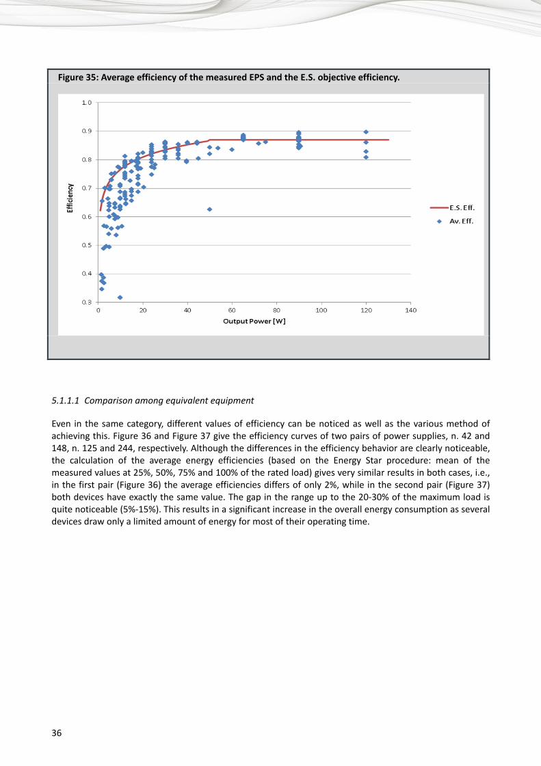
To be eligible for Energy Star qualification (class V), an external power supply model must meet or exceed a minimum average efficiency (mean of the measured values at 25%, 50%, 75% and 100% of the rated load), which varies based on the model’s nameplate output power, from 1 to 49W, according to the following equation: 0.063 ∗ ln 0.622

Where is the rated output power of the device. Beyond 49W the average efficiency must be ≥ 0.87. Figure 35 reports the average efficiencies of the measured adapters, with the objective efficiency curve based on Energy Star requirements and the ecodesign regulation for external power supplies (published in April 2009). It is interesting to note that only 75 EPSs are above that curve.

A: < 12 V B: 12V, ≤ 1 A C: 12V, 1 A < I ≤ 2 A D: 12V, 2 A < I ≤ 3.5 A E: 12V, 3.5 A < I ≤ 5 A F: >12V ÷ 18V G: ≥ 18V, Power ≤ 45W; H: ≥ 18V, 45W ÷ 70 W; I: ≥ 18V, 70W ÷ 95W; J: ≥ 18V, 95W ÷ 120 W;

36

Figure 35: Average efficiency of the measured EPS and the E.S. objective efficiency.

5.1.1.1 Comparison among equivalent equipment

Even in the same category, different values of efficiency can be noticed as well as the various method of achieving this. Figure 36 and Figure 37 give the efficiency curves of two pairs of power supplies, n. 42 and 148, n. 125 and 244, respectively. Although the differences in the efficiency behavior are clearly noticeable, the calculation of the average energy efficiencies (based on the Energy Star procedure: mean of the measured values at 25%, 50%, 75% and 100% of the rated load) gives very similar results in both cases, i.e., in the first pair (Figure 36) the average efficiencies differs of only 2%, while in the second pair (Figure 37) both devices have exactly the same value. The gap in the range up to the 20-30% of the maximum load is quite noticeable (5%-15%). This results in a significant increase in the overall energy consumption as several devices draw only a limited amount of energy for most of their operating time.

37

Figure 36: Energy efficiency curves with variable loads for a couple of adapters (42, blue line and 148, red line) with very similar average efficiencies.

Figure 37: Energy efficiency curves with variable loads for a couple of adapters (125, red line and 244, blue line) with the same average efficiency (0.869).

38

5.1.2 Efficiency at lower load – impact on some products

As stated previously, a considerable amount of equipment has quite variable energy consumption and draws only a limited amount of energy for most of its operating time, laptops for example. While the battery is fully charged and there is a low request for computational power, laptops would require a very low quantity of energy from the EPS. This condition is most common in the life of such devices. Table 2 shows the results of a survey of the amount of power (as a percentage of the EPS capability) a set of laptops consumes when in normal operation. It ranges from 16 to 29%.

Table 2: Normal operation (low performances) consumption.

PSU rating Consumption PSU utilization

W W %

Laptop 1 65 18 28% Laptop 2 65 14 22% Laptop 3 90 17 19% Laptop 4 65 19 29% Laptop 5 120 18.5 15% Laptop 6 120 19 16%

POS terminals are another example. Those terminals which populate shops, supermarkets and any modern cash register are normally into a quiescent, low power state, and turn into full activity (and consumption) only for the short time needed to process a payment.

A lot of energy is wasted as many power supplies are rather less efficient when the load is below 30%.

Remarks – Often, equivalent EPSs do show quite different efficiency at lower loads, while a lot of equipment have quite variable energy consumption and draw only a limited amount of energy for most of their operating time. The low-load efficiency difference results then in a significant increase in the overall energy consumption and should be avoided through optimizing the efficiency at 10-30% load.

Energy Star requires a power factor correction only for EPS rated 100W and above. In some other regions, such a requirement applies for EPSs when drawing an input power of 75W onward. The actual power factor is verified when the EPS is in a fully loaded condition.

Figure 38 shows the Cos φ values for all the analyzed power supplies. From the graph, it can be seen that almost every adapter with a high power factor value (more than 0.8) at 100% of the rated output power has a poor power factor when operating at lower power.

The graph in Figure 39 reports the energy efficiency and the power factor behavior versus the output loads of some adapters that have been not reported inside the previous figures, due to the apparent anomalous behavior of the efficiency curves. The efficiency values and the Cos φ values (Figure 39) have been coupled together to show that, in the range in which the efficiency has sudden changes in a strange manner, the Cos φ has a strong modification too. In this respect, these not conventional behaviors should depend on Cos φ control circuits. Figure 40 and Figure 41 report the same data for a single device each, to better clarify the above-described behavior. It can be argued that the power factor control mechanism described above is activated only when the load exceeds a predetermined threshold. This is probably aimed at obtaining good efficiency performances at lower output current values. Whenever the power factor control enters into action, this results into a clear reduction of the efficiency values which implies remarkable energy losses.

39

5.1.3 Power factor vs. load and efficiency

Figure 38: Cos ϕ curves with variable loads for all the analyzed adapters.

40

Figure 39: Energy efficiency and correlation with Cos φ curves for a set of adapters with some anomalous behaviors (not reported in the previous graphs).

41

Figure 40: Energy efficiency and Cos ϕ curves with variable loads for the adapter number 193.

Figure 41: Energy efficiency and Cos ϕ curves with variable loads for the adapter number 204.

42

Remarks – Many adapters having high power factor when at full load, actually show poor power factor at lower loads (Figure 38). As several devices (e.g., laptops) for most of the time draw only a minor amount of the rated energy of their power supplies, the above described behavior implies that, in real life, those EPSs will not benefit from the electrical network with a good power factor.

Designers and standard-makers should evaluate and specify the power factor limits also in the low load area where many devices operate for most of the time.

As the measurements have shown a severe negative correlation between the efficiency and power factor, this correlation should be evaluated in order to obtain the best overall effect.

5.2 Correlation between safety class and efficiency

Further analyses have shown another important aspect to be considered with respect to the safety class. As can be verified by analyzing Table 1, 65% of the entire set of considered power supplies belongs to safety class 2. Safety class 2 power supplies have to comply to much tougher requirements such as double insulation and increased resistibility to overvoltage, but this allows the use of the simpler, two pronged mains connector. The efficiency behavior of power supplies having the same ratings (voltage and current) but different safety classes have been compared so as to verify whether they could result into a different efficiency. In Figure 42, the blue lines identify a sub-set of safety class 2 adapters; red lines refer to safety class 1 adapter and solid and dotted lines identify groups of power supplies with the same name-plate characteristics.

Figure 42: Energy efficiency curves with variable loads for a subset of adapters belonging to safety class 1 (112, 116, 117, and 145, red lines) and 2 (102, 129, 143 and 146, blue lines). Solid lines and dotted lines identify devices with the same name plate characteristics.

43

Remarks – Figure 42 clearly underlines in both groups a better behavior of the devices belonging to safety class 2. Considering the savings of material, the better compatibility of the class 2 mains connectors (2 pins) and the increased safety for clients, it might be advisable the complete switch-over to this kind of solution/connectors/cables.

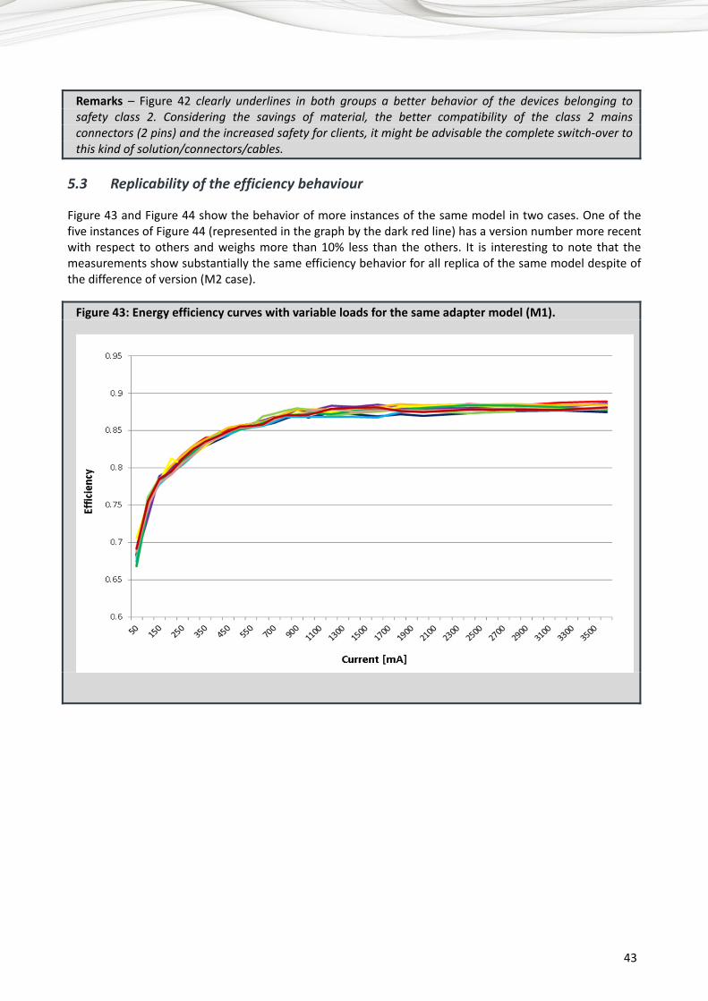
5.3 Replicability of the efficiency behaviour

Figure 43 and Figure 44 show the behavior of more instances of the same model in two cases. One of the five instances of Figure 44 (represented in the graph by the dark red line) has a version number more recent with respect to others and weighs more than 10% less than the others. It is interesting to note that the measurements show substantially the same efficiency behavior for all replica of the same model despite of the difference of version (M2 case).

Figure 43: Energy efficiency curves with variable loads for the same adapter model (M1).

44

Figure 44: Energy efficiency curves with variable loads for the same adapter model (M2).

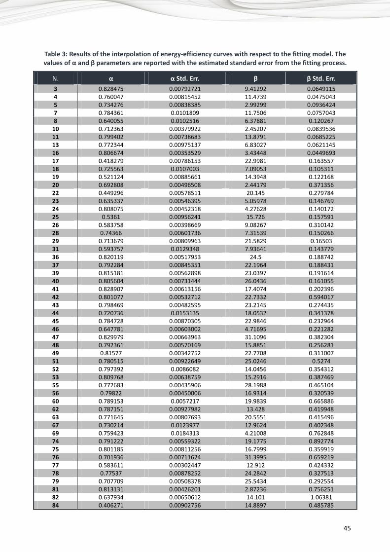
5.4 Analytical analysis

In order to synthetically describe the energy-aware performance of EPS, it was decided to fit the collected samples of the characteristic curves in Figure 22 with the following function: 1

Where i represent the value of the provided DC current, and α and β are the fitting parameters. In more detail, α obviously represents the maximum efficiency achievable by the adapter and the β parameter gives an indication on how fast the maximum efficiency levels are achieved.

For example, for having an efficiency correspondent to the 97% of α level for I > 150 mA, β values must be greater than 23.37. In this respect, the percentage of devices with β > 23.37 is only the 24% corresponding to 49 elements.

Table 3 reports α and β parameters, and the related standard error, obtained by fitting the characteristic curves of each charger in Figure 22 with the above model introduced. Standard errors clearly give useful feedbacks on the goodness of the fitting itself, but also on the regularity of the curve slopes.

45

Table 3: Results of the interpolation of energy-efficiency curves with respect to the fitting model. The values of α and β parameters are reported with the estimated standard error from the fitting process.

N. α α Std. Err. β β Std. Err. 3 0.828475 0.00792721 9.41292 0.06491154 0.760047 0.00815452 11.4739 0.04750435 0.734276 0.00838385 2.99299 0.09364247 0.784361 0.0101809 11.7506 0.07570438 0.640055 0.0102516 6.37881 0.120267

10 0.712363 0.00379922 2.45207 0.083953611 0.799402 0.00738683 13.8791 0.068522513 0.772344 0.00975137 6.83027 0.062114516 0.806674 0.00353529 3.43448 0.044969317 0.418279 0.00786153 22.9981 0.16355718 0.725563 0.0107003 7.09053 0.10531119 0.521124 0.00885661 14.3948 0.12216820 0.692808 0.00496508 2.44179 0.37135622 0.449296 0.00578511 20.145 0.27978423 0.635337 0.00546395 5.05978 0.14676924 0.808075 0.00452318 4.27628 0.14017225 0.5361 0.00956241 15.726 0.15759126 0.583758 0.00398669 9.08267 0.31014228 0.74366 0.00601736 7.31539 0.15026629 0.713679 0.00809963 21.5829 0.1650331 0.593757 0.0129348 7.93641 0.14377936 0.820119 0.00517953 24.5 0.18874237 0.792284 0.00845351 22.1964 0.18843139 0.815181 0.00562898 23.0397 0.19161440 0.805604 0.00731444 26.0436 0.16105541 0.828907 0.00613156 17.4074 0.20239642 0.801077 0.00532712 22.7332 0.59401743 0.798469 0.00482595 23.2145 0.27443544 0.720736 0.0153135 18.0532 0.34137845 0.784728 0.00870305 22.9846 0.23296446 0.647781 0.00603002 4.71695 0.22128247 0.829979 0.00663963 31.1096 0.38230448 0.792361 0.00570169 15.8851 0.25628149 0.81577 0.00342752 22.7708 0.31100751 0.780515 0.00922649 25.0246 0.527452 0.797392 0.0086082 14.0456 0.35431253 0.809768 0.00638759 15.2916 0.38746955 0.772683 0.00435906 28.1988 0.46510456 0.79822 0.00450006 16.9314 0.32053960 0.789153 0.0057217 19.9839 0.66588662 0.787151 0.00927982 13.428 0.41994863 0.771645 0.00807693 20.5551 0.41549667 0.730214 0.0123977 12.9624 0.40234869 0.759423 0.0184313 4.21008 0.76284874 0.791222 0.00559322 19.1775 0.89277475 0.801185 0.00811256 16.7999 0.35991976 0.701936 0.00711624 31.3995 0.65921977 0.583611 0.00302447 12.912 0.42433278 0.77537 0.00878252 24.2842 0.32751379 0.707709 0.00508378 25.5434 0.29255481 0.813131 0.00426201 2.87236 0.75625182 0.637934 0.00650612 14.101 1.0638184 0.406271 0.00902756 14.8897 0.485785

46

N. α α Std. Err. β β Std. Err. 85 0.762992 0.0095617 11.9738 0.37812587 0.829481 0.00454196 7.95591 0.70878788 0.699798 0.0057159 24.9962 0.74238793 0.571693 0.0161706 17.6126 1.1861697 0.485003 0.00852096 22.4556 1.19495

102 0.827712 0.00623694 20.0199 0.697187103 0.759485 0.0140135 9.826 0.62796105 0.791485 0.00797301 18.7977 1.02141106 0.616347 0.0108985 8.14188 0.656876108 0.639556 0.00469357 4.91567 0.988827109 0.811402 0.00683158 12.4946 0.580141110 0.706564 0.00740594 4.91486 0.985254111 0.77482 0.00847748 14.0373 1.11063112 0.76444 0.00561523 11.6541 0.820046113 0.662326 0.0120936 4.59278 1.41294114 0.680114 0.0124106 4.21554 4.0453115 0.667779 0.0114156 7.07564 0.671815116 0.716614 0.00878702 6.44441 0.309103117 0.718559 0.0100749 6.78707 1.29335119 0.773021 0.00776199 14.315 0.913909120 0.714856 0.0059122 4.69044 0.682191121 0.8107 0.00346362 3.30847 0.755531123 0.815304 0.00429707 6.03414 1.11041125 0.84723 0.00818185 11.3621 1.09665128 0.819805 0.00643603 18.5675 0.889387129 0.812869 0.00596295 14.1344 0.866879131 0.751942 0.0081181 12.1497 1.46766132 0.877029 0.00424362 18.785 1.47612137 0.491784 0.0062617 24.9168 1.05118141 0.838809 0.00582058 15.06 1.2134142 0.856862 0.00634797 10.3901 1.2249143 0.740453 0.0114916 14.8056 1.46364145 0.742973 0.00884431 5.74094 1.55763146 0.739559 0.0123469 15.1667 1.22424147 0.813042 0.00449029 2.96506 1.1791148 0.807232 0.00638411 6.77028 1.69608149 0.783994 0.00783526 4.2907 1.64649150 0.790631 0.00907248 14.4919 1.21552151 0.77588 0.00756108 4.26062 1.05496152 0.729218 0.0113791 15.9129 1.07996153 0.600049 0.00571926 8.39505 1.12094154 0.691209 0.00847967 14.2977 1.71222157 0.624381 0.00867833 15.2207 1.13238158 0.825889 0.00994343 7.4924 1.40321159 0.693395 0.00490523 17.5654 0.816726163 0.405762 0.0393367 12.6807 0.770721165 0.662798 0.00622483 34.8857 1.1521167 0.556428 0.00735982 12.4535 0.786705168 0.845809 0.00739747 7.178 1.33129169 0.780357 0.0050706 6.437 0.909983170 0.603631 0.0112969 6.55527 2.47641171 0.7856 0.00445291 21.5897 1.58199172 0.449997 0.00956217 8.26225 0.963235173 0.810147 0.00461753 23.9131 2.47846174 0.63996 0.00703489 25.1189 3.04335175 0.854751 0.00499255 25.24 1.10997

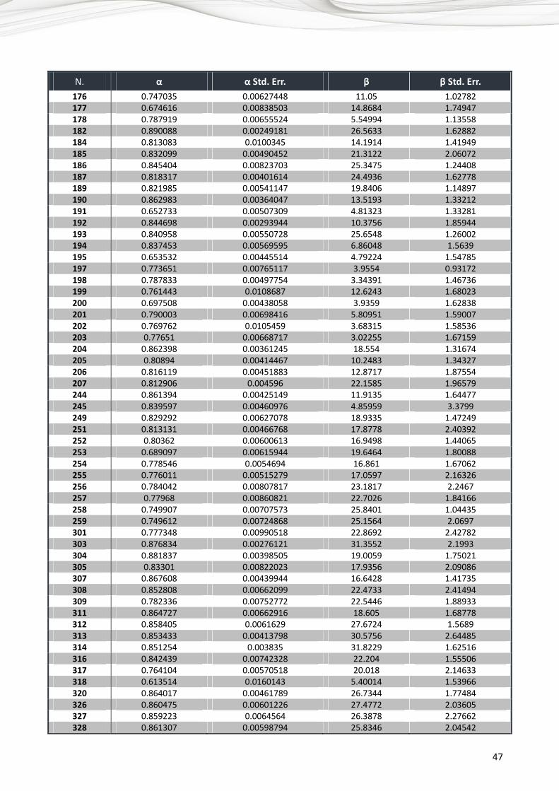
47

N. α α Std. Err. β β Std. Err. 176 0.747035 0.00627448 11.05 1.02782177 0.674616 0.00838503 14.8684 1.74947178 0.787919 0.00655524 5.54994 1.13558182 0.890088 0.00249181 26.5633 1.62882184 0.813083 0.0100345 14.1914 1.41949185 0.832099 0.00490452 21.3122 2.06072186 0.845404 0.00823703 25.3475 1.24408187 0.818317 0.00401614 24.4936 1.62778189 0.821985 0.00541147 19.8406 1.14897190 0.862983 0.00364047 13.5193 1.33212191 0.652733 0.00507309 4.81323 1.33281192 0.844698 0.00293944 10.3756 1.85944193 0.840958 0.00550728 25.6548 1.26002194 0.837453 0.00569595 6.86048 1.5639195 0.653532 0.00445514 4.79224 1.54785197 0.773651 0.00765117 3.9554 0.93172198 0.787833 0.00497754 3.34391 1.46736199 0.761443 0.0108687 12.6243 1.68023200 0.697508 0.00438058 3.9359 1.62838201 0.790003 0.00698416 5.80951 1.59007202 0.769762 0.0105459 3.68315 1.58536203 0.77651 0.00668717 3.02255 1.67159204 0.862398 0.00361245 18.554 1.31674205 0.80894 0.00414467 10.2483 1.34327206 0.816119 0.00451883 12.8717 1.87554207 0.812906 0.004596 22.1585 1.96579244 0.861394 0.00425149 11.9135 1.64477245 0.839597 0.00460976 4.85959 3.3799249 0.829292 0.00627078 18.9335 1.47249251 0.813131 0.00466768 17.8778 2.40392252 0.80362 0.00600613 16.9498 1.44065253 0.689097 0.00615944 19.6464 1.80088254 0.778546 0.0054694 16.861 1.67062255 0.776011 0.00515279 17.0597 2.16326256 0.784042 0.00807817 23.1817 2.2467257 0.77968 0.00860821 22.7026 1.84166258 0.749907 0.00707573 25.8401 1.04435259 0.749612 0.00724868 25.1564 2.0697301 0.777348 0.00990518 22.8692 2.42782303 0.876834 0.00276121 31.3552 2.1993304 0.881837 0.00398505 19.0059 1.75021305 0.83301 0.00822023 17.9356 2.09086307 0.867608 0.00439944 16.6428 1.41735308 0.852808 0.00662099 22.4733 2.41494309 0.782336 0.00752772 22.5446 1.88933311 0.864727 0.00662916 18.605 1.68778312 0.858405 0.0061629 27.6724 1.5689313 0.853433 0.00413798 30.5756 2.64485314 0.851254 0.003835 31.8229 1.62516316 0.842439 0.00742328 22.204 1.55506317 0.764104 0.00570518 20.018 2.14633318 0.613514 0.0160143 5.40014 1.53966320 0.864017 0.00461789 26.7344 1.77484326 0.860475 0.00601226 27.4772 2.03605327 0.859223 0.0064564 26.3878 2.27662328 0.861307 0.00598794 25.8346 2.04542

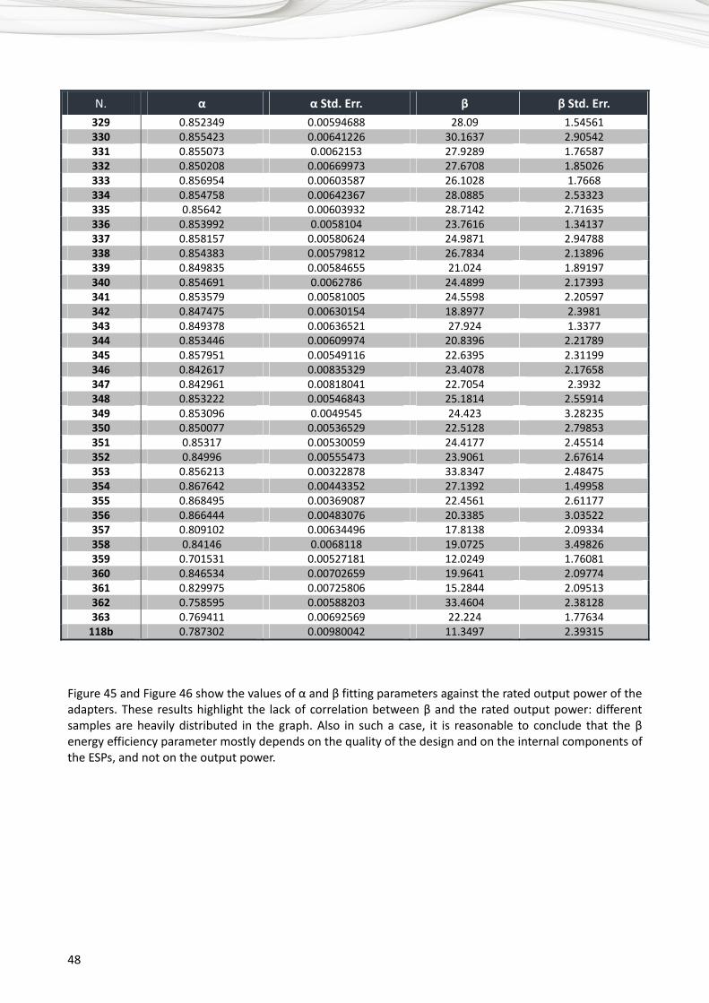
48

N. α α Std. Err. β β Std. Err. 329 0.852349 0.00594688 28.09 1.54561330 0.855423 0.00641226 30.1637 2.90542331 0.855073 0.0062153 27.9289 1.76587332 0.850208 0.00669973 27.6708 1.85026333 0.856954 0.00603587 26.1028 1.7668334 0.854758 0.00642367 28.0885 2.53323335 0.85642 0.00603932 28.7142 2.71635336 0.853992 0.0058104 23.7616 1.34137337 0.858157 0.00580624 24.9871 2.94788338 0.854383 0.00579812 26.7834 2.13896339 0.849835 0.00584655 21.024 1.89197340 0.854691 0.0062786 24.4899 2.17393341 0.853579 0.00581005 24.5598 2.20597342 0.847475 0.00630154 18.8977 2.3981343 0.849378 0.00636521 27.924 1.3377344 0.853446 0.00609974 20.8396 2.21789345 0.857951 0.00549116 22.6395 2.31199346 0.842617 0.00835329 23.4078 2.17658347 0.842961 0.00818041 22.7054 2.3932348 0.853222 0.00546843 25.1814 2.55914349 0.853096 0.0049545 24.423 3.28235350 0.850077 0.00536529 22.5128 2.79853351 0.85317 0.00530059 24.4177 2.45514352 0.84996 0.00555473 23.9061 2.67614353 0.856213 0.00322878 33.8347 2.48475354 0.867642 0.00443352 27.1392 1.49958355 0.868495 0.00369087 22.4561 2.61177356 0.866444 0.00483076 20.3385 3.03522357 0.809102 0.00634496 17.8138 2.09334358 0.84146 0.0068118 19.0725 3.49826359 0.701531 0.00527181 12.0249 1.76081360 0.846534 0.00702659 19.9641 2.09774361 0.829975 0.00725806 15.2844 2.09513362 0.758595 0.00588203 33.4604 2.38128363 0.769411 0.00692569 22.224 1.77634

118b 0.787302 0.00980042 11.3497 2.39315

Figure 45 and Figure 46 show the values of α and β fitting parameters against the rated output power of the adapters. These results highlight the lack of correlation between β and the rated output power: different samples are heavily distributed in the graph. Also in such a case, it is reasonable to conclude that the β energy efficiency parameter mostly depends on the quality of the design and on the internal components of the ESPs, and not on the output power.

49

Figure 45: Values from the α parameter as in Table 3.

Figure 46: Values from the β parameter as in Table 3.

50

Remarks – The analytical analysis with alpha and beta parameters indicates that only the 24% of the power supplies reach its efficiency target value at low output current. This would result into a very relevant increase in the overall energy consumption as several devices draw only limited amount of energy for a significant amount of time. It is interesting to note that, among these 49 “good” devices, 42 are rated in Energy Star class V or IV.

Figure 47 represents the correlation between weight and efficiency results. The graph shows the values of power density with respect to weight (without cable), versus β values, for the best adapters in terms of efficiency (α > 0.85). In the figure, a green and a red line highlight respectively a β and a power density constraint above which a power supply has quite a satisfactory behavior. In the area beyond these constraints, a subset of 17 EPSs that show high efficiency and a large W/g ratio can be found.

Figure 47: Power density with respect to weight (without cable), versus β values for a subset of adapters with α > 0.85.

Remarks – As Figure 47 underlines, a good compromise between weight and efficiency can be reached. This suggests again the opportunity of design improvements for a large part of current devices.

5.5 Output voltage

The graphs in the following figures report the DC voltage provided by the analyzed set of power supplies according to the output current. In such a case, it can be underlined how some power supplies, which declare a nameplate DC voltage value, provide different voltage values in some parts of the measurement range. Moreover, in some other cases, the voltage levels decrease considerably according to output current.

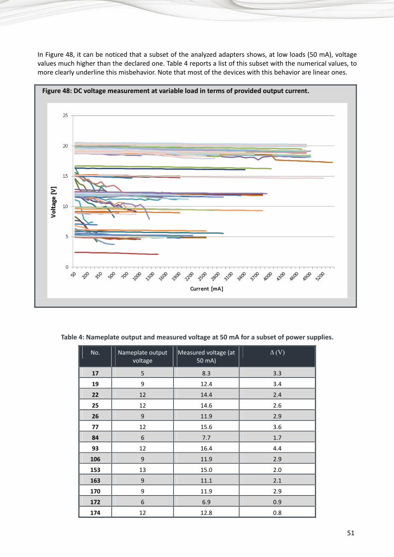
51

In Figure 48, it can be noticed that a subset of the analyzed adapters shows, at low loads (50 mA), voltage values much higher than the declared one. Table 4 reports a list of this subset with the numerical values, to more clearly underline this misbehavior. Note that most of the devices with this behavior are linear ones.

Figure 48: DC voltage measurement at variable load in terms of provided output current.

Table 4: Nameplate output and measured voltage at 50 mA for a subset of power supplies.

No. Nameplate output voltage

Measured voltage (at 50 mA)

Δ (V)

17 5 8.3 3.3

19 9 12.4 3.4

22 12 14.4 2.4

25 12 14.6 2.6

26 9 11.9 2.9

77 12 15.6 3.6

84 6 7.7 1.7

93 12 16.4 4.4

106 9 11.9 2.9

153 13 15.0 2.0

163 9 11.1 2.1

170 9 11.9 2.9

172 6 6.9 0.9

174 12 12.8 0.8

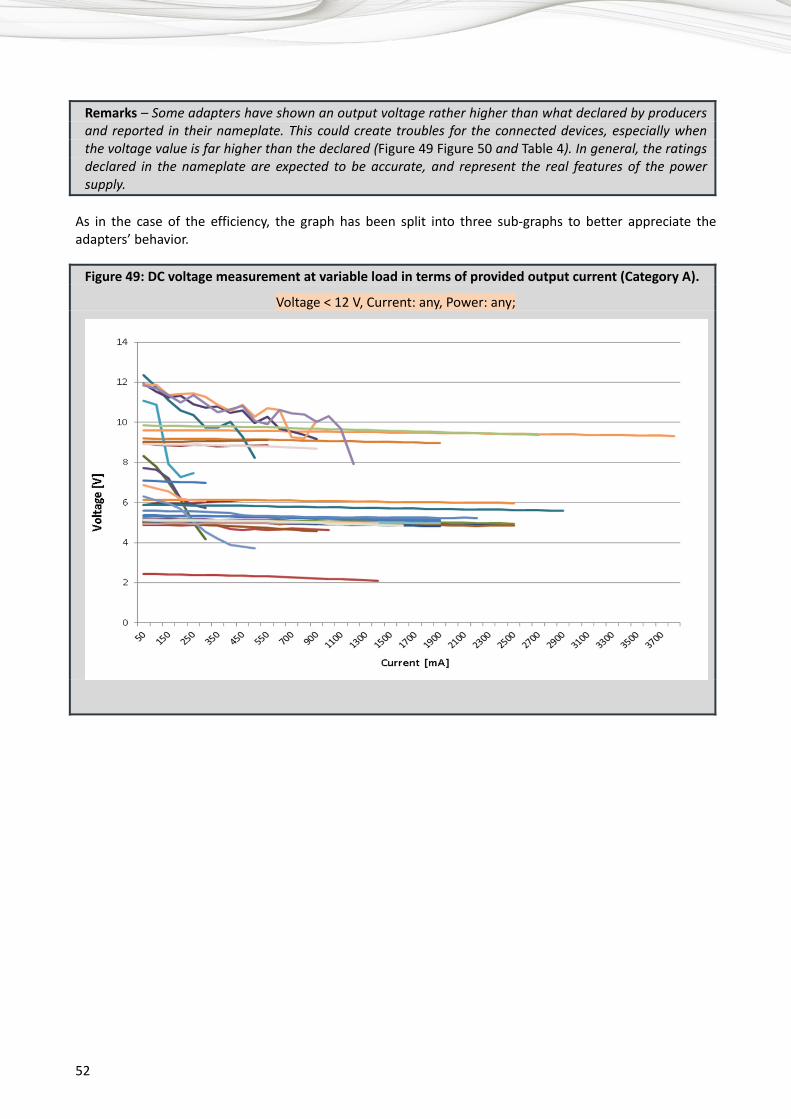
52

Remarks – Some adapters have shown an output voltage rather higher than what declared by producers and reported in their nameplate. This could create troubles for the connected devices, especially when the voltage value is far higher than the declared (Figure 49 Figure 50 and Table 4). In general, the ratings declared in the nameplate are expected to be accurate, and represent the real features of the power supply.

As in the case of the efficiency, the graph has been split into three sub-graphs to better appreciate the adapters’ behavior.

Figure 49: DC voltage measurement at variable load in terms of provided output current (Category A).

Voltage < 12 V, Current: any, Power: any;

53

Figure 50: DC voltage measurement at variable load in terms of provided output current (Category B).

Voltage = 12V, Current ≤ 1 A, Power: any;

Figure 51: DC voltage measurement at variable load in terms of provided output current (Category C).

Voltage = 12V, 1 A < Current ≤ 2 A, Power: any;

54

Figure 52: DC voltage measurement at variable load in terms of provided output current (Category D).

Voltage = 12V, 2 A < Current ≤ 3.5 A, Power: any;

Figure 53: DC voltage measurement at variable load in terms of provided output current (Category E).

Voltage = 12V, 3.5 A < Current ≤ 5 A, Power: any;

55

Figure 54: DC voltage measurement at variable load in terms of provided output current (Category F).

12 V < Voltage < 18V, Current: any, Power: any;

Figure 55: DC voltage measurement at variable load in terms of provided output current (Category G).

Voltage ≥ 18V, Current: any, Power ≤ 45W;

56

Figure 56: DC voltage measurement at variable load in terms of provided output current (Category H).

Voltage ≥ 18V, Current: any, 45W < Power ≤ 70 W;

Figure 57: DC voltage measurement at variable load in terms of provided output current (Category I).

Voltage ≥ 18V, Current: any, 70W < Power ≤ 95W;

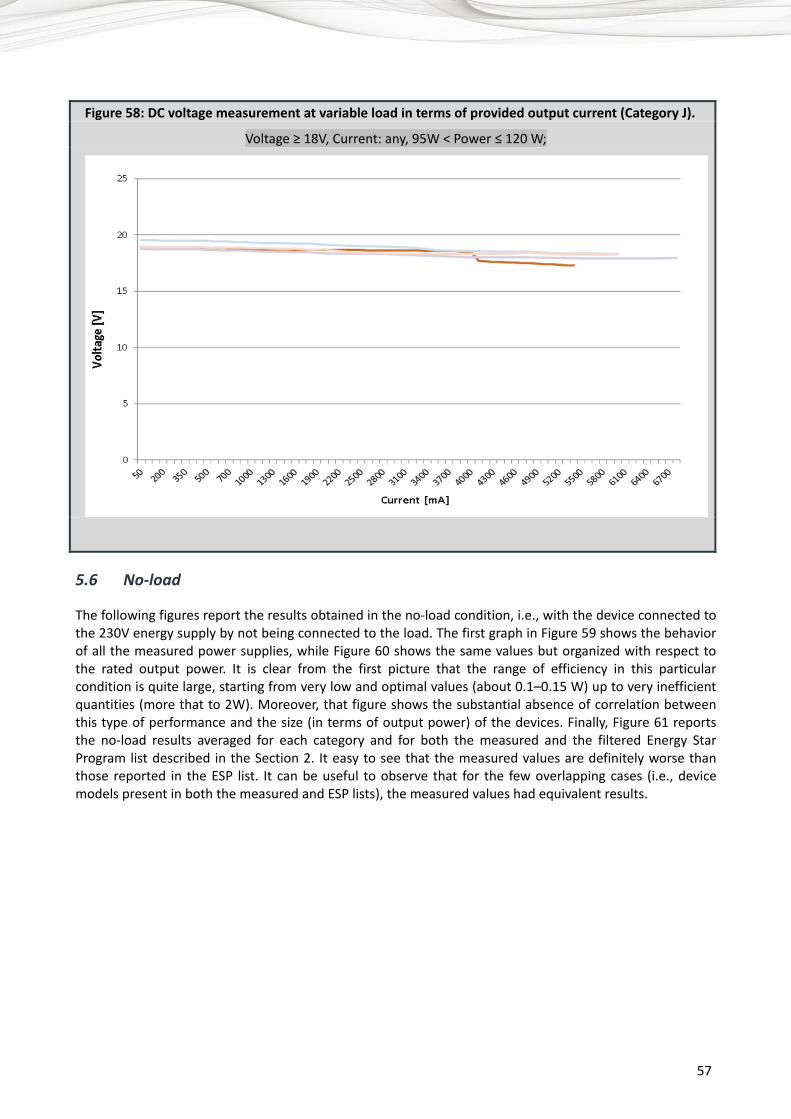
57

Figure 58: DC voltage measurement at variable load in terms of provided output current (Category J).

Voltage ≥ 18V, Current: any, 95W < Power ≤ 120 W;

5.6 No-load

The following figures report the results obtained in the no-load condition, i.e., with the device connected to the 230V energy supply by not being connected to the load. The first graph in Figure 59 shows the behavior of all the measured power supplies, while Figure 60 shows the same values but organized with respect to the rated output power. It is clear from the first picture that the range of efficiency in this particular condition is quite large, starting from very low and optimal values (about 0.1–0.15 W) up to very inefficient quantities (more that to 2W). Moreover, that figure shows the substantial absence of correlation between this type of performance and the size (in terms of output power) of the devices. Finally, Figure 61 reports the no-load results averaged for each category and for both the measured and the filtered Energy Star Program list described in the Section 2. It easy to see that the measured values are definitely worse than those reported in the ESP list. It can be useful to observe that for the few overlapping cases (i.e., device models present in both the measured and ESP lists), the measured values had equivalent results.

58

Figure 59: No-load absorbed power [W] of all the measured power supplies.

Remarks – The large range of no-load efficiency clearly demonstrated by Figure 59 and Figure 60, together with the substantial absence of correlation between this quantity and output power, contribute again to suggest large opportunities of obtaining better average performances.

59

Figure 60: No load absorbed power [W] versus the rated output power for all the measured devices.

Figure 61: No load average absorbed power [W] versus categories for the measured and the ESP list devices.

A: < 12 V B: 12V, ≤ 1 A C: 12V, 1 A < I ≤ 2 A D: 12V, 2 A < I ≤ 3.5 A E: 12V, 3.5 A < I ≤ 5 A F: >12V ÷ 18V G: ≥ 18V, Power ≤ 45W; H: ≥ 18V, 45W ÷ 70 W; I: ≥ 18V, 70W ÷ 95W; J: ≥ 18V, 95W ÷ 120 W;

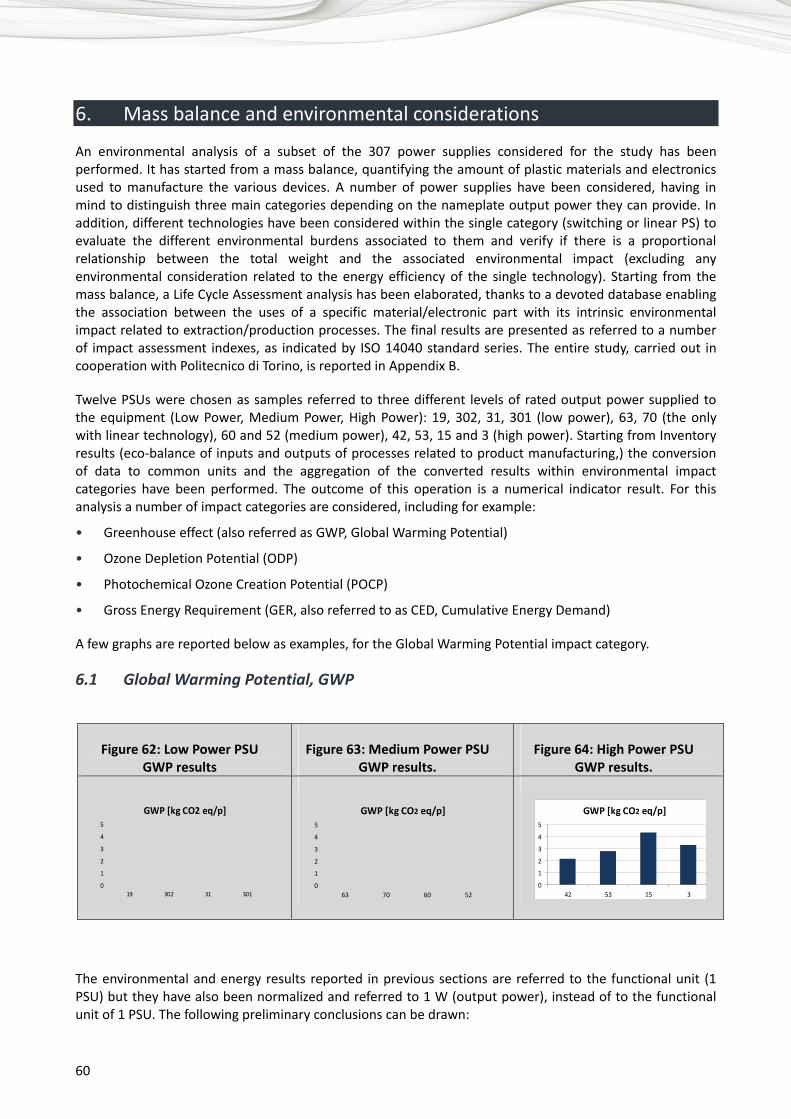
60

6. Mass balance and environmental considerations

An environmental analysis of a subset of the 307 power supplies considered for the study has been performed. It has started from a mass balance, quantifying the amount of plastic materials and electronics used to manufacture the various devices. A number of power supplies have been considered, having in mind to distinguish three main categories depending on the nameplate output power they can provide. In addition, different technologies have been considered within the single category (switching or linear PS) to evaluate the different environmental burdens associated to them and verify if there is a proportional relationship between the total weight and the associated environmental impact (excluding any environmental consideration related to the energy efficiency of the single technology). Starting from the mass balance, a Life Cycle Assessment analysis has been elaborated, thanks to a devoted database enabling the association between the uses of a specific material/electronic part with its intrinsic environmental impact related to extraction/production processes. The final results are presented as referred to a number of impact assessment indexes, as indicated by ISO 14040 standard series. The entire study, carried out in cooperation with Politecnico di Torino, is reported in Appendix B.

Twelve PSUs were chosen as samples referred to three different levels of rated output power supplied to the equipment (Low Power, Medium Power, High Power): 19, 302, 31, 301 (low power), 63, 70 (the only with linear technology), 60 and 52 (medium power), 42, 53, 15 and 3 (high power). Starting from Inventory results (eco-balance of inputs and outputs of processes related to product manufacturing,) the conversion of data to common units and the aggregation of the converted results within environmental impact categories have been performed. The outcome of this operation is a numerical indicator result. For this analysis a number of impact categories are considered, including for example:

• Greenhouse effect (also referred as GWP, Global Warming Potential)

• Ozone Depletion Potential (ODP)

• Photochemical Ozone Creation Potential (POCP)

• Gross Energy Requirement (GER, also referred to as CED, Cumulative Energy Demand)

A few graphs are reported below as examples, for the Global Warming Potential impact category.

6.1 Global Warming Potential, GWP

Figure 62: Low Power PSU GWP results

Figure 63: Medium Power PSU GWP results.

Figure 64: High Power PSU GWP results.

The environmental and energy results reported in previous sections are referred to the functional unit (1 PSU) but they have also been normalized and referred to 1 W (output power), instead of to the functional unit of 1 PSU. The following preliminary conclusions can be drawn:

0

1

2

3

4

5

42 53 15 3

GWP [kg CO2 eq/p]

0

1

2

3

4

5

63 70 60 52

GWP [kg CO2 eq/p]

0

1

2

3

4

5

19 302 31 301

GWP [kg CO2 eq/p]

61

• Environmental and energy impacts do not depend only on weight characteristics; the behavior also depend on the different design choices especially for the electronics, and is at any rate different depending on the single impact category analyzed;

• Environmental and energetic impacts do not depend only on output power. In some cases, high power PSU has very similar impacts in comparison to medium power PSU, and the same applies to the comparison between the medium power and low power category. This fact demonstrates the importance of adopting accurate design choices (especially for electronics, but also for the plastics) for minimizing the environmental burdens associated to the single product;

• Within the same impact category, it is always possible to identify one example of PSU coupling good use-performance as well as good environmental and energetic performances. Depending on the single impact categories, the best in class for the single category can improve the performances of the worst one of a mean percentage around 25-30%, up to 50% in some specific cases. Again, this demonstrates the importance of adopting design rules optimizing the environmental aspects.

A more detailed analysis of the general up-described framework should be necessary in order to assess how the environmental impacts depend on the design of electronics as well as on the design of the object (in terms of material selection).

7. Conclusions

In general, this work shows that there are many aspects where an aggressive standardization action can act in the direction of safety, better customer usage and, especially, better performance with respect to the environmental impact. More specifically, the main indications of this study can be summarized in the following points:

• Only 47% shows the ES label and, moreover, this label is found very seldom in lower power adapters (< 40W).However, low power adapters constitute an important part of the market and both the absence of the ES label and the efficiency measurement results indicate poor efficiency values for many of these devices. This point suggests the presence of a serious problem and it seems to be not in line with the conclusions of the Energy Star Programme (i.e., the market was already mature and capable to behave autonomously as per the EPS requirements).

• It can be easily noticed that voltage, current and especially power values seem to tend to common ratings. This fact makes one think of a kind of “de facto” standardization. This condition is particularly evident in two specific cases: The low voltage connectors: the five most used connector types represent 86 % of the total The output voltage: where the large majority of the devices (81%) have an output voltage of 5, 12 or

19 V.

• Adapters with a very different output voltage often have the same connector type. This creates further confusion among users and could generate problems and risks for the users in case they would use one of them to power different products. An evaluation should be done to decide on whether it would be better to standardize the use of the existing connectors defined by HGI and ETSI, or to define new connectors (one for each category) such us the ones under study in other standardization activities.

• A high dispersion on weights of adapters having the same ratings has been demonstrated. In particular for the lower power equipment, there is a substantial independence between weight and power, with the higher power equipment appearing to be more aligned amongst each other and showing a sort of linear dependence between power and weight. Moreover, there is a huge difference between the best and the worst adapter, in terms of weight, for each category. For most of the categories, the percentage of power supplies that weigh more than the best plus the 20% is very large. As weight can be directly linked to the environmental impact, it would be advisable to urge manufacturers to consider this issue and optimize their products aligning to other already achieved.

62

• Because of the weight of the charger is relatively high for portable computers and for portable devices and because the main cause of failure on all portable devices is the weak point at the output of the power supply, it is highly recommended to have a detachable cable on the DC side allowing replacement. This confirms the need for standardizing connectors for each family of devices to avoid errors, unless a sufficiently reliable configuration protocol can be standardized.

• Combining market data and measured weight, it is clear that a huge quantity of material could be saved. A cautious estimate indicates that the aggregated amount, if electronics of EPSs is 1 million tons per year, is growing. At least half of it could be expected to be saved if a standardized solution is available. Because weight is directly linked to environmental impact, it would be advisable to urge manufacturers to optimize their products, aligning them with the best (lightest) in the corresponding category as it could reduce the use of resources (and e-waste) by 300 thousand tons per year.

• As for efficiency versus the output current, a high dispersion of adapter efficiencies both in general and inside the same class has been underlined by the measurements. This aspect suggests an important opportunity of improving the efficiency characteristics independently from their power capacity.

• Often, equivalent EPSs do show quite different efficiency at lower loads, while a lot of equipment have quite variable energy consumption and draw only a limited amount of energy for most of their operating time. The low-load efficiency difference results then in a significant increase in the overall energy consumption and should be avoided through optimizing the efficiency at 10-30% load.

• Many adapters having high power factor when at full load actually show poor power factor at lower loads (Figure 38). As several devices (e.g., laptops) for most of the time draw only a minor amount of the rated energy of their power supplies, the above described behavior implies that, in real life, those EPSs will not from benefit the electrical network with good power factor. Designers and standardizers should evaluate and specify the power factor limits also in low load areas where many devices operate for most of the time.

• The analytical analysis with alpha and beta parameters indicates that only 24% of the power supplies reach their efficiency target value at low output current. This would result into a very relevant increase in the overall energy consumption as several devices draw only a limited amount of energy for a significant amount of time.

• As the measurements have shown a severe negative correlation between the efficiency and power factor, it should be evaluated which is the most import in order to obtain the best overall effect.

• The devices belonging to safety class 2 have a better efficiency behavior. Considering the savings of material, the better compatibility of the class 2 mains connectors (2 pins) and the increased safety for clients, it might be advisable to switch over completely to this kind of solution/connectors/cables.

• Some adapters have shown an output voltage rather higher than what is declared by producers and reported in their nameplate. This could create problems for the connected devices, especially when the voltage value is far higher than what is declared. In general, the ratings declared in the nameplate are expected to be accurate, and represent the real features of the power supply.

• The range of no-load efficiency is quite large, starting from very low and optimal values (about 0.1–0.15 W) up to very inefficient quantities (more that to 2W). Moreover, there is substantial absence of correlation between this type of performance and the size (in terms of output power) of the devices. Finally, the no-load results averaged for each category are definitely worse than those reported in the ESP list. These observations again suggest large opportunities of obtaining better average performances.

• The environmental analysis performed on a subset of devices included in the study shows that the dependency between environmental impacts and weight or output power characteristics is partial; this fact demonstrates the importance of adopting accurate design choices (especially for electronics, but also for the plastics) for minimizing the environmental burdens associated to the single product. Furthermore, within the same impact category, it is always possible to identify one example of PSU

63

coupling good use-performance as well as good environmental and energetic performances. Depending on the single impact categories, the best in classes can improve the performances of the worst ones of a mean percentage around 25-30%, up to 50% in some specific cases. Again, this demonstrates the importance of adopting design rules optimizing the environmental aspects; a more detailed analysis should be necessary in order to evaluate in detail the single sources of impact that are causing the highlighted differences.

ITU-T Study Group 5 (SG5), which is responsible for studying ICT environmental aspects of electromagnetic phenomena and climate change, is currently discussing the development of a recommendation which would provide high level requirements for a universal common power supply solution for ICT devices.

The aim would be to reduce the number of power adapters and chargers produced and recycled by widening their application to more devices and by increasing their lifetime. The solution would also aim to reduce energy consumption.

8. References • Bolla R., Bruschi R., D’Agostino L. – An Energy-aware Survey on Mobile-Phone Chargers

• L.adapter phase2 – efficiency versus load and equipment behavior

• ENERGY STAR External Power Supplies AC-DC Product List, December 2010

• Darnell - External AC-DC Power Supplies: Economic Factors, Application Drivers, Architecture/Packaging Trends, Technology and Regulatory Developments - Tenth Edition

• Darnell - AC-DC Power Supplies: Worldwide Forecasts - Tenth Edition

64

9. Appendix A

9.1 Test bed

This section introduces the description of the test bed used to measure the electrical features of the devices analyzed. The accuracy obtained is considered consistent with the test aims (mainly for comparison purposes among equipment).

Figure 65 shows the set-up test bed. The power supplies have been connected to a Hameg HM 8115-2 power-meter, to measure:

• Apparent Power = VA = S

• Reactive Power = Var = Q

• Active Power = W = P

From these values, Power Factor = Cos φ = PF = P/S can be determined.

Figure 65: Measurements test bed.

As can be seen in Figure 65, the output of the power adapter has been connected to the H&H ZS 506-4 Electronic load. Through this device, the load applied to the adapter can be changed modifying the current drawn.

To obtain efficiency curves, the current has been increased from 50 mA to 600 mA with steps of 50mA and from 600 mA to the declared maximum power of every power adapter with steps of 100 mA. Together with the change of current increment also the resolution of the measurements has been changed.

65

10. Appendix B

LIFE CYCLE ASSESSMENT METHODOLOGY APPLIED TO POWER SUPPLIES FOR CUSTOMER PREMISES EQUIPMENT *

* Appendix B is currently being updated in order to comply with Recommendation ITU-T L.1410, which had

not yet been approved at the time of writing of this appendix.

Politecnico di Torino - Dipartimento di Scienza dei Materiali ed Ingegneria Chimica

Corso Duca degli Abruzzi, 24 - 10129 Torino – Italy

www.polito.it

in cooperation with:

Life Cycle Engineering - Studio Ingegneri Associati (Studio LCE), TORINO - Italy

www.studiolce.it

POLITECNICO DI TORINO

Prof. Bruno De Benedetti

Ing. Paolo Tecchio

Dott.ssa Sara Rollino

LIFE CYCLE ENGINEERING

Ing. Gian Luca Baldo

66

Table of contents

1 Introduction ........................................................................................................................................ 67 1.1 Analyzed products ...................................................................................................................... 67 1.2 Data collection procedure .......................................................................................................... 67 1.3 Framework of the report ............................................................................................................ 68

2 Goal definition and scoping ................................................................................................................ 69 2.1 Goal and scope definition ........................................................................................................... 69 2.2 Functional unit ............................................................................................................................ 69 2.3 System boundaries ..................................................................................................................... 69 2.4 Data categories ........................................................................................................................... 70 2.5 Data quality requirements .......................................................................................................... 70

3 Life Cycle Inventory (LCI)..................................................................................................................... 71 3.1 Low power PSU ........................................................................................................................... 71 3.2 Medium power PSU .................................................................................................................... 72 3.3 High power PSU .......................................................................................................................... 72

4 Life Cycle Impact Assessment ............................................................................................................. 73 4.1 Emissions classification and characterization ............................................................................. 74 4.2 Impact categories ....................................................................................................................... 74 4.3 Classification and characterization results ................................................................................. 75

5 Interpretation ..................................................................................................................................... 85 5.1 Contributors to Low power PSU ................................................................................................. 86 5.2 Contributors to Medium power PSU .......................................................................................... 87 5.3 Contributors to High power PSU ................................................................................................ 88 5.4 LCIA referred to the maximum output power ............................................................................ 89

6 Preliminary Conclusions ..................................................................................................................... 94

7 References .......................................................................................................................................... 95

8 Acronyms & Symbols .......................................................................................................................... 95

9 Appendix: Environmental Indicators .................................................................................................. 96 9.1 Environmental indicators ............................................................................................................ 96

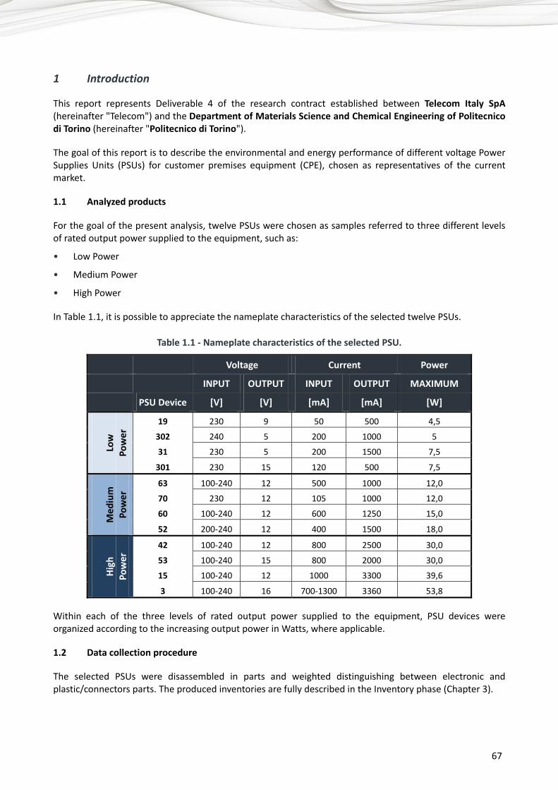
67

1 Introduction

This report represents Deliverable 4 of the research contract established between Telecom Italy SpA (hereinafter "Telecom") and the Department of Materials Science and Chemical Engineering of Politecnico di Torino (hereinafter "Politecnico di Torino").

The goal of this report is to describe the environmental and energy performance of different voltage Power Supplies Units (PSUs) for customer premises equipment (CPE), chosen as representatives of the current market.

1.1 Analyzed products

For the goal of the present analysis, twelve PSUs were chosen as samples referred to three different levels of rated output power supplied to the equipment, such as:

• Low Power

• Medium Power

• High Power

In Table 1.1, it is possible to appreciate the nameplate characteristics of the selected twelve PSUs.

Table 1.1 - Nameplate characteristics of the selected PSU.

Voltage Current Power

INPUT OUTPUT INPUT OUTPUT MAXIMUM

PSU Device [V] [V] [mA] [mA] [W]

Low

Po

wer

19 230 9 50 500 4,5

302 240 5 200 1000 5

31 230 5 200 1500 7,5

301 230 15 120 500 7,5

Med

ium

Po

wer

63 100-240 12 500 1000 12,0

70 230 12 105 1000 12,0

60 100-240 12 600 1250 15,0

52 200-240 12 400 1500 18,0

High

Po

wer

42 100-240 12 800 2500 30,0

53 100-240 15 800 2000 30,0

15 100-240 12 1000 3300 39,6

3 100-240 16 700-1300 3360 53,8

Within each of the three levels of rated output power supplied to the equipment, PSU devices were organized according to the increasing output power in Watts, where applicable.

1.2 Data collection procedure

The selected PSUs were disassembled in parts and weighted distinguishing between electronic and plastic/connectors parts. The produced inventories are fully described in the Inventory phase (Chapter 3).

68

1.3 Framework of the report

The Ecodesign considers product and service following a Life Cycle Thinking approach: product designers are called to select design pathways not only according to material and performance criteria, but also from the energy and environmental burdens of these selections. This is the reason why the framework of this report follows the indications provided by the ISO 14040 and 14044 Standards. In order to facilitate the approach within the mentioned framework of standards and to unify the way of reporting within this LCA study, each phase of the report is introduced by a technical brief definition provided by the specific standard.

The following figure shows a general scheme of the LCA methodology as provided by ISO 14040: each main phase reported in the figure is then briefly introduced.

Figure 1.1 - The LCA structure defined by the ISO 14040

Inventory

ImpactAssessment

LCA FRAMEWORK

ISO 14040:2006

Goal and scope

ISO 14044:2006

Goal and definition of scope: it is the preliminary phase in which the aim of the study, the functional unit, the system boundaries, the data categories, the assumptions and the limits are defined.

Life Cycle Inventory: it is the main section of the work, dedicated to the study of the life cycle of the system product. This phase is mainly concerned with the data collection and calculation procedures. The goal is to provide a detailed description (operational model) of the raw materials and fuels entering the system (inputs) as well as solid, liquid and gaseous waste exiting the system (outputs). A software tool is normally used to support the modeling procedures and to provide database information.

Life Cycle Impact Assessment: it assists the understanding of Inventory results, making them more manageable in relation to the natural environment, human health and resources and may identify the relative significance of the Inventory results.

Life Cycle Interpretation: it is the conclusive phase of a LCA study in which the findings of either the Inventory or the Impact Assessment or both are combined with the defined goal and scope in order to

69

reach conclusions and formulate recommendations. Once the improvements concerning the considered system have been suggested or implemented, the inventory is performed again to see if the expected changes have occurred but also to identify if any unwanted side effects have accidentally been introduced.

A glossary, an overview on calculation procedures and the meaning of terms used to describe the LCA results are reported in the Appendix.

2 Goal, definition and scope

2.1 Goal and definition of scope

The goal and scope of an LCA shall be clearly defined and shall be consistent with the intended application. Due to the iterative nature of LCA, the scope may have to be refined during the study. In defining the goal of an LCA, the following items shall be unambiguously stated: the intended application, the reasons for carrying out the study, the intended audience, i.e. to whom the results of the study are intended to be communicated, and whether the results are intended to be used in comparative assertions intended to be disclosed to the public. In defining the scope of an LCA, the following items shall be considered and clearly described: the product system to be studied; the functions of the product system or, in the case of comparative studies, the systems; the functional unit; the system boundary; allocation procedures; impact categories selected and methodology of impact assessment, and subsequent interpretation to be used; data requirements; assumptions; limitations; initial data quality requirements; type of critical review, if any; type and format of the report required for the study. (ISO 14044:2006, Par. 4.2.2 – 4.2.3).

The aims of this study are:

• To develop the assessment of the environmental burden for the implemented materials used to make twelve PSUs by means of the Ecodesign approach.

• To organize the LCA results in a standard way, according to ISO 14044:2006 and to the needs of Telecom Italy.

2.2 Functional unit

The functional unit defines the quantification of the identified functions (performance characteristics) of the product. The primary purpose of a functional unit is to provide a reference to which the inputs and outputs are related. This reference is necessary to ensure comparability of LCA results. Comparability of LCA results is particularly critical when different systems are being assessed, to ensure that such comparisons are made on a common basis. It is important to determine the reference flow in each product system, in order to fulfill the intended function i.e. the amount of products needed to fulfill the function (ISO 14040:2006, Par. 5.2.2).

The function of the considered system is one PSU.

2.3 System boundaries

The system boundary defines the unit processes to be included in the system. Ideally, the product system should be modeled in such a manner that inputs and outputs at its boundary are elementary flows. However, resources need not be expended on the quantification of such inputs and outputs that will not significantly change the overall conclusions of the study. (ISO 14040: 2006, Par. 5.2.3).

The boundaries of the system include materials and components used in the PSU production phase.

The present study does not include in the system boundaries the phases of assembly in the factory, packaging & transport, use phase and end of life.

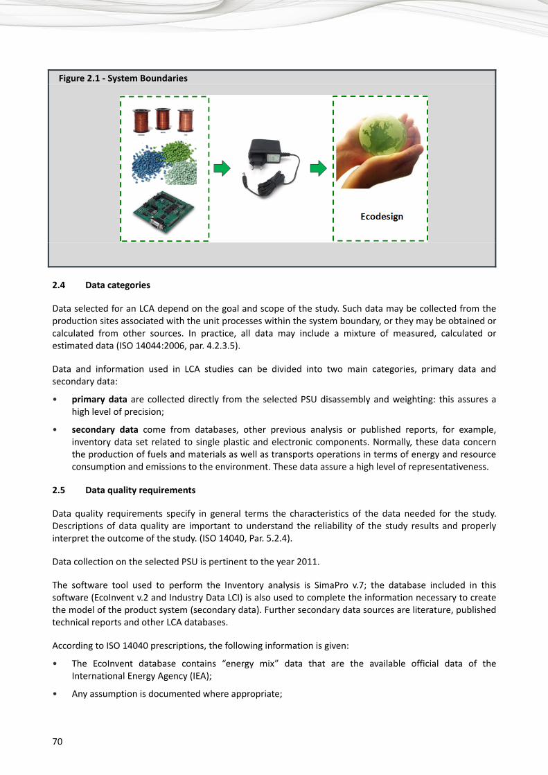
70

Figure 2.1 - System Boundaries

2.4 Data categories

Data selected for an LCA depend on the goal and scope of the study. Such data may be collected from the production sites associated with the unit processes within the system boundary, or they may be obtained or calculated from other sources. In practice, all data may include a mixture of measured, calculated or estimated data (ISO 14044:2006, par. 4.2.3.5).

Data and information used in LCA studies can be divided into two main categories, primary data and secondary data:

• primary data are collected directly from the selected PSU disassembly and weighting: this assures a high level of precision;

• secondary data come from databases, other previous analysis or published reports, for example, inventory data set related to single plastic and electronic components. Normally, these data concern the production of fuels and materials as well as transports operations in terms of energy and resource consumption and emissions to the environment. These data assure a high level of representativeness.

2.5 Data quality requirements

Data quality requirements specify in general terms the characteristics of the data needed for the study. Descriptions of data quality are important to understand the reliability of the study results and properly interpret the outcome of the study. (ISO 14040, Par. 5.2.4).

Data collection on the selected PSU is pertinent to the year 2011.

The software tool used to perform the Inventory analysis is SimaPro v.7; the database included in this software (EcoInvent v.2 and Industry Data LCI) is also used to complete the information necessary to create the model of the product system (secondary data). Further secondary data sources are literature, published technical reports and other LCA databases.

According to ISO 14040 prescriptions, the following information is given:

• The EcoInvent database contains “energy mix” data that are the available official data of the International Energy Agency (IEA);

• Any assumption is documented where appropriate;

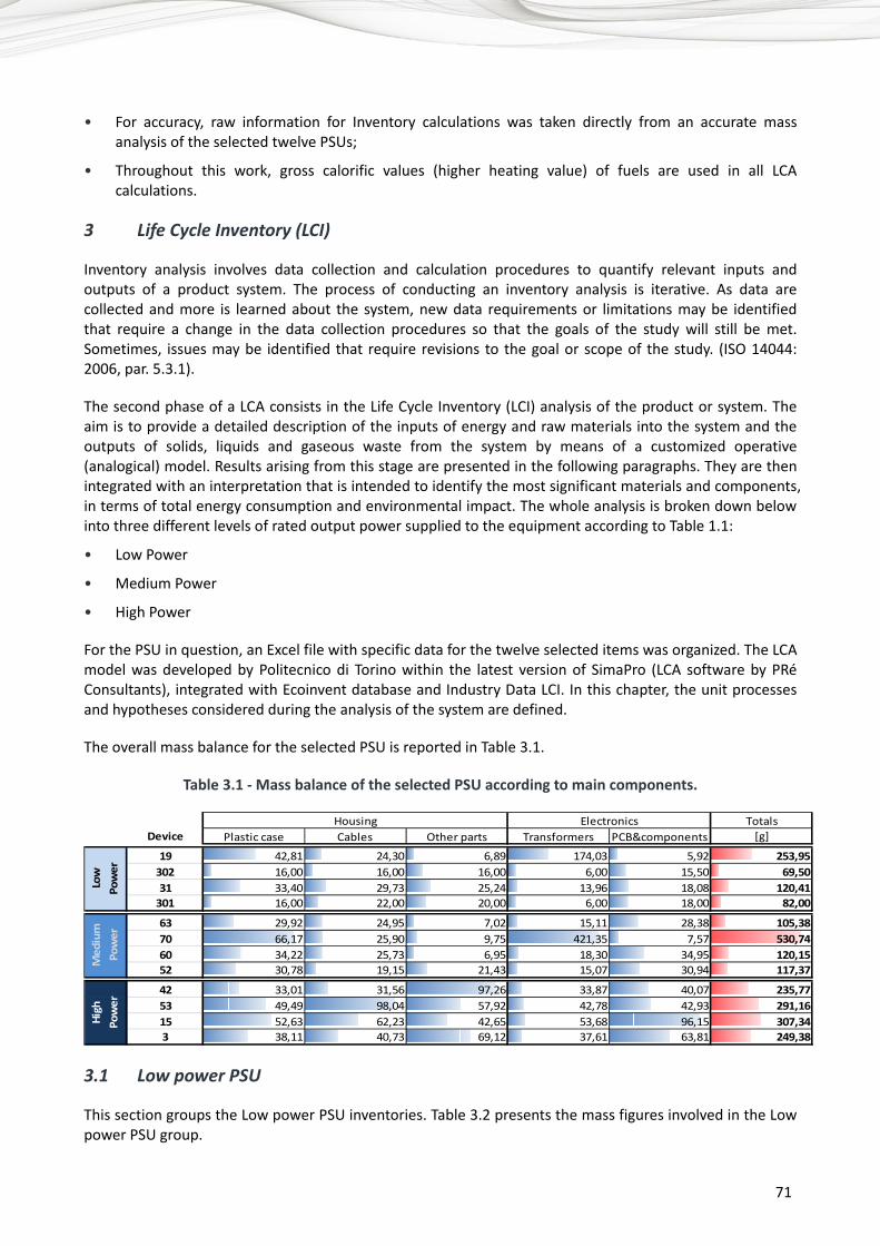
71

• For accuracy, raw information for Inventory calculations was taken directly from an accurate mass analysis of the selected twelve PSUs;

• Throughout this work, gross calorific values (higher heating value) of fuels are used in all LCA calculations.

3 Life Cycle Inventory (LCI)

Inventory analysis involves data collection and calculation procedures to quantify relevant inputs and outputs of a product system. The process of conducting an inventory analysis is iterative. As data are collected and more is learned about the system, new data requirements or limitations may be identified that require a change in the data collection procedures so that the goals of the study will still be met. Sometimes, issues may be identified that require revisions to the goal or scope of the study. (ISO 14044: 2006, par. 5.3.1).

The second phase of a LCA consists in the Life Cycle Inventory (LCI) analysis of the product or system. The aim is to provide a detailed description of the inputs of energy and raw materials into the system and the outputs of solids, liquids and gaseous waste from the system by means of a customized operative (analogical) model. Results arising from this stage are presented in the following paragraphs. They are then integrated with an interpretation that is intended to identify the most significant materials and components, in terms of total energy consumption and environmental impact. The whole analysis is broken down below into three different levels of rated output power supplied to the equipment according to Table 1.1:

• Low Power

• Medium Power

• High Power

For the PSU in question, an Excel file with specific data for the twelve selected items was organized. The LCA model was developed by Politecnico di Torino within the latest version of SimaPro (LCA software by PRé Consultants), integrated with Ecoinvent database and Industry Data LCI. In this chapter, the unit processes and hypotheses considered during the analysis of the system are defined.

The overall mass balance for the selected PSU is reported in Table 3.1.

Table 3.1 - Mass balance of the selected PSU according to main components.

TotalsDevice Plastic case Cables Other parts Transformers PCB&components [g]

19 42,81 24,30 6,89 174,03 5,92 253,95302 16,00 16,00 16,00 6,00 15,50 69,5031 33,40 29,73 25,24 13,96 18,08 120,41

301 16,00 22,00 20,00 6,00 18,00 82,00

63 29,92 24,95 7,02 15,11 28,38 105,3870 66,17 25,90 9,75 421,35 7,57 530,7460 34,22 25,73 6,95 18,30 34,95 120,1552 30,78 19,15 21,43 15,07 30,94 117,37

42 33,01 31,56 97,26 33,87 40,07 235,7753 49,49 98,04 57,92 42,78 42,93 291,1615 52,63 62,23 42,65 53,68 96,15 307,343 38,11 40,73 69,12 37,61 63,81 249,38

Housing Electronics

Low

Po

wer

Med

ium

Po

wer

High

Po

wer

3.1 Low power PSU

This section groups the Low power PSU inventories. Table 3.2 presents the mass figures involved in the Low power PSU group.

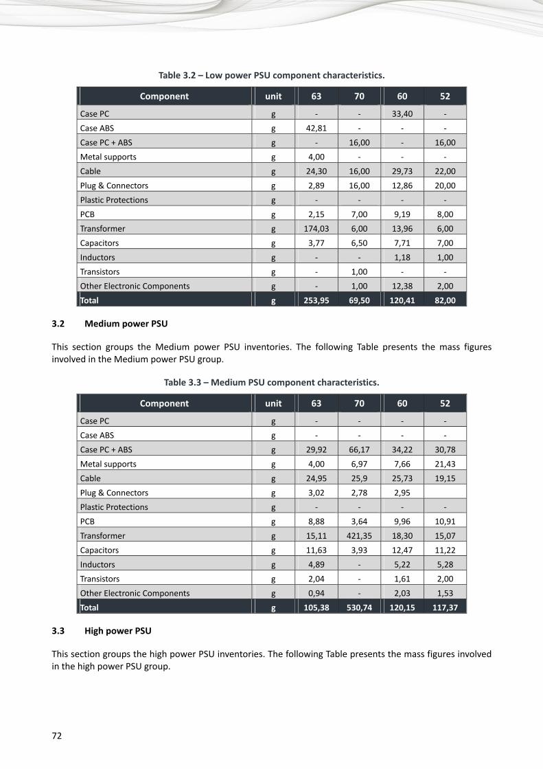
72

Table 3.2 – Low power PSU component characteristics.

Component unit 63 70 60 52

Case PC g - - 33,40 - Case ABS g 42,81 - - - Case PC + ABS g - 16,00 - 16,00 Metal supports g 4,00 - - - Cable g 24,30 16,00 29,73 22,00 Plug & Connectors g 2,89 16,00 12,86 20,00 Plastic Protections g - - - - PCB g 2,15 7,00 9,19 8,00 Transformer g 174,03 6,00 13,96 6,00 Capacitors g 3,77 6,50 7,71 7,00 Inductors g - - 1,18 1,00 Transistors g - 1,00 - - Other Electronic Components g - 1,00 12,38 2,00 Total g 253,95 69,50 120,41 82,00

3.2 Medium power PSU

This section groups the Medium power PSU inventories. The following Table presents the mass figures involved in the Medium power PSU group.

Table 3.3 – Medium PSU component characteristics.

Component unit 63 70 60 52

Case PC g - - - - Case ABS g - - - - Case PC + ABS g 29,92 66,17 34,22 30,78 Metal supports g 4,00 6,97 7,66 21,43 Cable g 24,95 25,9 25,73 19,15 Plug & Connectors g 3,02 2,78 2,95 Plastic Protections g - - - - PCB g 8,88 3,64 9,96 10,91 Transformer g 15,11 421,35 18,30 15,07 Capacitors g 11,63 3,93 12,47 11,22 Inductors g 4,89 - 5,22 5,28 Transistors g 2,04 - 1,61 2,00 Other Electronic Components g 0,94 - 2,03 1,53 Total g 105,38 530,74 120,15 117,37

3.3 High power PSU

This section groups the high power PSU inventories. The following Table presents the mass figures involved in the high power PSU group.

73

Table 3.4 – High PSU component characteristics.

Component unit 42 53 15 3

Case PC g - - - 38,11 Case ABS g - - - - Case PC + ABS g 33,01 49,49 52,63 - Metal supports g 14,52 25,39 23,88 48,34 Cable g 79,72 98,04 62,23 40,73 Plug & Connectors g 34,58 32,53 18,26 10,14 Plastic Protections g - - 0,51 10,64 PCB g 14,34 14,60 29,94 18,87 Transformer g 33,87 42,78 53,68 37,61 Capacitors g 22,21 19,99 29,31 26,38 Inductors g 2,01 3,88 31,40 11,75 Transistors g 1,00 2,00 4,20 3,39 Other Electronic Components g 0,51 2,46 1,30 3,42 Total g 235,77 291,16 307,34 249,38

Subsequently, data from Table 3.2, Table 3.3 and Table 3.4 have been organized to build a LCA model for each PSU, by means of the SimaPro software. EcoInvent database (which contains international industrial life cycle inventory data on energy supply, resource extraction, air emissions, water emissions and solid waste flows) has been used to match each single item of the inventories with a dataset, mainly in the field of electronic components and devices, plastics and metals. For each material and component available in the software, it is possible to know the environmental impacts. As a result, it is also possible to calculate all PSUs final impact assessments which are presented in the following chapter.

4 Life Cycle Impact Assessment

The impact assessment phase of LCA is aimed at evaluating the significance of potential environmental impacts using the LCI results. In general, this process involves associating inventory data with specific environmental impact categories and category indicators, thereby attempting to understand these impacts. The LCIA phase also provides information for the life cycle interpretation phase. The impact assessment may include the iterative process of reviewing the goal and scope of the LCA study to determine if the objectives of the study have been met, or to modify the goal and scope if the assessment indicates that they cannot be achieved. Issues such as choice, modelling and evaluation of impact categories can introduce subjectivity into the LCIA phase. Therefore, transparency is critical to the impact assessment to ensure that assumptions are clearly described and reported. (ISO 14040, par. 5.4.1).

According to ISO 14044 Standard schematically reported in Figure 4.1, the general framework of the Assessment phase is composed of several mandatory elements that convert Inventory results to environmental indicators. In addition, there are optional elements for grouping, transformation of the indicator results and data quality assessment techniques.

74

Figure 4.1 – Main steps of the Impact Assessment phase

Life Cycle Impact Assessment phase

Mandatoryelements

Impact categories definition

LCI results assignation (classification)

Category indicator calculation (characterisation)

Optional elements

Comparison with a standard value (normalisation)

Grouping

Weighting

ISO 14044:2006

4.1 Emission classification and characterization

Classification is the assignment of Inventory results to impact categories whereas characterization involves the calculation of category indicator results, which means the conversion of Inventory results to common units and the aggregation of the converted results within the impact categories. The outcome of this operation is a numerical indicator result.

4.2 Impact categories

Emission classification and characterization are respectively based on the definition of some environmental impact potentials and, moreover, on the calculation of a numerical indicator resulting on the base of a characterization factor.

For this analysis, the following impact categories3 are considered:

• Greenhouse effect (also referred as GWP, Global Warming Potential)

• Ozone Depletion Potential (ODP)

• Photochemical Ozone Creation Potential (POCP)

• Acidification Potential (AP)

• Eutrophication Potential (EP)

• Gross Energy Requirement (GER, also referred as CED, Cumulative Energy Demand)

• Water use

3 A brief description of each impact category is available in Appendix.

75

4.3 Classification and characterization results

The results of the classification and characterization phases, calculated by using the environmental indicators of the previous paragraph and the general rules reported in the Appendix, are presented in the following table.

Table 4.1 - Environmental and energy results.

IMPACT CATEGORY Low power Medium power High power

19 302 31 301 63 70 60 52 42 53 15 3

GWP [kg CO2 eq/p]

1,15 1,03 1,58 1,28 1,50 2,28 1,98 2,13 2,19 2,80 4,37 3,33

ODP [kg CFC-11 eq/p]

5,8E-08 6,7E-08 1,8E-07 9,8E-08 9,3E-08 1,1E-07 1,3E-07 1,5E-07 1,4E-07 1,7E-07 2,8E-07 2,2E-07

POCP [kg C2H4 eq/p]

0,0017 0,0029 0,0049 0,0026 0,0059 0,0028 0,0057 0,0055 0,0075 0,0080 0,0161 0,0111

AP [kg SO2 eq/p]

0,0078 0,0279 0,0447 0,0232 0,0533 0,0161 0,0463 0,0425 0,0638 0,0641 0,1148 0,0801

EP [kg PO4 3– eq/p]

0,0007 0,0006 0,0010 0,0008 0,0008 0,0014 0,0010 0,0013 0,0012 0,0015 0,0024 0,0019

GER [MJ/p]

22,85 20,92 29,57 25,20 30,2 43,0 39,8 42,1 44,8 57,5 87,5 64,5

Water use [kg/p]

9,72 12,07 20,77 13,31 18,7 19,1 22,8 23,8 25,2 31,0 54,1 40,9

4.3.1 Global Warming Potential, GWP

Figure 4.2 – Low Power PSU GWP results.

0,00

1,00

2,00

3,00

4,00

5,00

19 302 31 301

GWP [kg CO2 eq/p]

76

Figure 4.3 – Medium Power PSU GWP results.

0,00

1,00

2,00

3,00

4,00

5,00

63 70 60 52

GWP [kg CO2 eq/p]

Figure 4.4 – High Power PSU GWP results.

0,00

1,00

2,00

3,00

4,00

5,00

42 53 15 3

GWP [kg CO2 eq/p]

77

4.3.2 Ozone Depletion Potential, ODP

Figure 4.5 – Low Power PSU ODP results.

0,0E+00

5,0E-08

1,0E-07

1,5E-07

2,0E-07

2,5E-07

3,0E-07

19 302 31 301

ODP [kg CFC-11 eq/p]

Figure 4.6 – Medium Power PSU ODP results.

0,0E+00

5,0E-08

1,0E-07

1,5E-07

2,0E-07

2,5E-07

3,0E-07

63 70 60 52

ODP [kg CFC-11 eq/p]

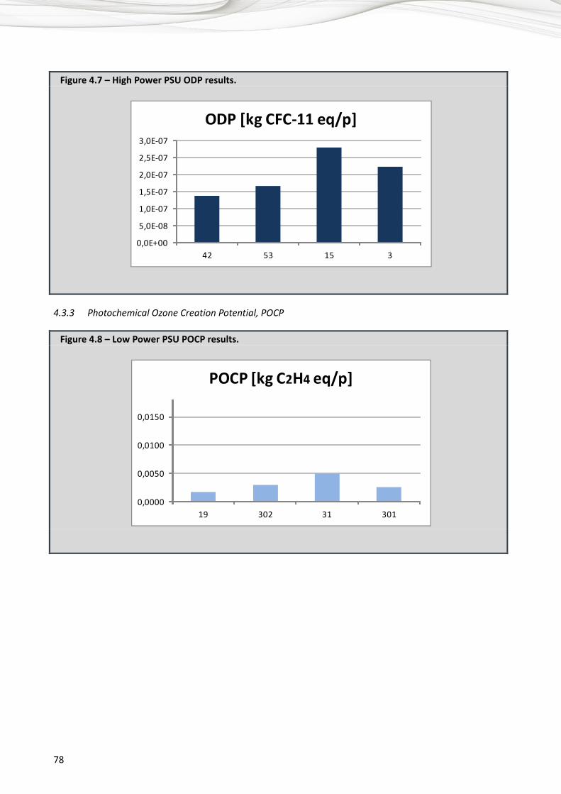
78

Figure 4.7 – High Power PSU ODP results.

0,0E+00

5,0E-08

1,0E-07

1,5E-07

2,0E-07

2,5E-07

3,0E-07

42 53 15 3

ODP [kg CFC-11 eq/p]

4.3.3 Photochemical Ozone Creation Potential, POCP

Figure 4.8 – Low Power PSU POCP results.

0,0000

0,0050

0,0100

0,0150

19 302 31 301

POCP [kg C2H4 eq/p]

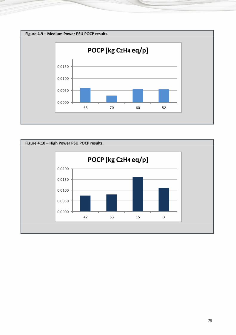
79

Figure 4.9 – Medium Power PSU POCP results.

0,0000

0,0050

0,0100

0,0150

63 70 60 52

POCP [kg C2H4 eq/p]

Figure 4.10 – High Power PSU POCP results.

0,0000

0,0050

0,0100

0,0150

0,0200

42 53 15 3

POCP [kg C2H4 eq/p]

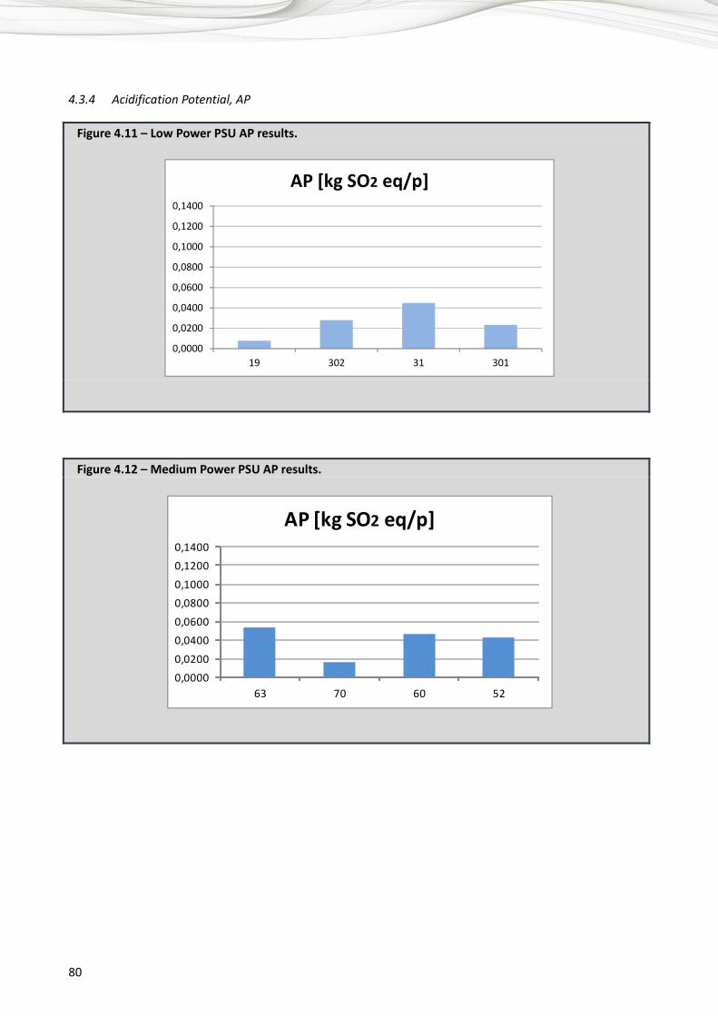
80

4.3.4 Acidification Potential, AP

Figure 4.11 – Low Power PSU AP results.

0,0000

0,0200

0,0400

0,0600

0,0800

0,1000

0,1200

0,1400

19 302 31 301

AP [kg SO2 eq/p]

Figure 4.12 – Medium Power PSU AP results.

0,00000,02000,04000,06000,08000,10000,12000,1400

63 70 60 52

AP [kg SO2 eq/p]

81

Figure 4.13 – High Power PSU AP results.

0,00000,02000,04000,06000,08000,10000,12000,1400

42 53 15 3

AP [kg SO2 eq/p]

4.3.5 Eutrophication Potential, EP

Figure 4.14 – Low Power PSU EP results.

0,0000

0,0005

0,0010

0,0015

0,0020

0,0025

19 302 31 301

EP [kg PO4 3– eq/p]

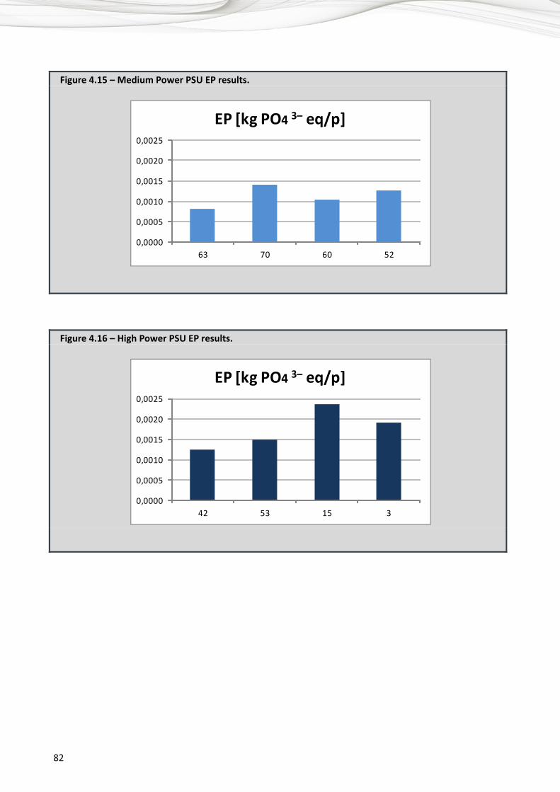
82

Figure 4.15 – Medium Power PSU EP results.

0,0000

0,0005

0,0010

0,0015

0,0020

0,0025

63 70 60 52

EP [kg PO4 3– eq/p]

Figure 4.16 – High Power PSU EP results.

0,0000

0,0005

0,0010

0,0015

0,0020

0,0025

42 53 15 3

EP [kg PO4 3– eq/p]

83

4.3.6 Gross Energy Requirement, GER

Figure 4.17 – Low Power PSU GER results.

0,00

20,00

40,00

60,00

80,00

100,00

19 302 31 301

GER [MJ/p]

Figure 4.18 – Medium Power PSU GER results.

0,0

20,0

40,0

60,0

80,0

100,0

63 70 60 52

GER [MJ/p]

84

Figure 4.19 – High Power PSU GER results.

0,0

20,0

40,0

60,0

80,0

100,0

42 53 15 3

GER [MJ/p]

4.3.7 Water use

Figure 4.20 – Low Power PSU Water Use results.

0,00

10,00

20,00

30,00

40,00

50,00

60,00

19 302 31 301

Water use [kg/p]

85

Figure 4.21 – Medium Power PSU Water Use results.

0,0

10,0

20,0

30,0

40,0

50,0

60,0

63 70 60 52

Water use [kg/p]

Figure 4.22 – High Power PSU Water Use results.

0,0

10,0

20,0

30,0

40,0

50,0

60,0

42 53 15 3

Water use [kg/p]

5 Interpretation

Interpretation is the phase of LCA in which the findings from the inventory analysis and the impact assessment are considered together or, in the case of LCI studies, the findings of the inventory analysis only. The interpretation phase should deliver results that are consistent with the defined goal and scope and which reach conclusions, explain limitations and provide recommendations. The interpretation should reflect the fact that the LCIA results are based on a relative approach, that they indicate potential environmental effects, and that they do not predict actual impacts on category endpoints, the exceeding of thresholds or safety margins or risks. The findings of this interpretation may take the form of conclusions and recommendations to decision-makers, consistent with the goal and scope of the study. Life cycle interpretation is also intended to provide a readily understandable, complete and consistent presentation of the results of an LCA, in accordance with the goal and scope definition of the study. The interpretation

86

phase may involve the iterative process of reviewing and revising the scope of the LCA, as well as the nature and quality of the data collected in a way which is consistent with the defined goal. (ISO 14040, Par. 5.5).

Life Cycle Assessment results might be used for several purposes: as a base for process improvement, products innovation, according to sustainable production, or the development of an environmental policy strategy.

In this report, environmental impacts have been organized for the purposes of the study addressed to ITU according to High, Medium and Low Power PSU categories. In the following paragraphs, it is possible to appreciate the contributors to the environmental indicators (GWP, ODP, POCP, AP, EP, GER, Water use) according to the following main areas:

• Plastic Case

• Cables

• Other Parts

• Transformers

• PCB & components

The following graphs show the percentage contribution of these five areas to each environmental indicator, referred to the total figures of Table 4.1.

5.1 Contributors to Low power PSU

Figure 5.1 – Share-out of GWP, ODP, POCP, AP, EP, GER, Water use among the reported main

components of the 302 PSUs.

Figure 5.2 – Share-out of GWP, ODP, POCP, AP, EP, GER, Water use among the reported main

components of the 301 PSUs.

0% 20% 40% 60% 80% 100%

GWP

ODP

POCP

AP

EP

GER

Water use

GWP ODP POCP AP EP GER Wateruse

Plastic case 9% 3% 3% 1% 5% 10% 2%Cables 4% 2% 3% 2% 5% 5% 3%Other parts 8% 6% 2% 1% 6% 8% 4%Transformers 2% 2% 1% 1% 3% 2% 2%PCB&components 77% 88% 91% 95% 81% 75% 88%

302 - Contributors to indicators

0% 20% 40% 60% 80% 100%

GWP

ODP

POCP

AP

EP

GER

Water use

GWP ODP POCP AP EP GER Water use

Plastic case 7% 2% 4% 1% 4% 8% 2%Cables 5% 2% 5% 3% 4% 6% 4%Other parts 8% 5% 3% 2% 5% 8% 5%Transformers 2% 1% 1% 1% 2% 2% 2%PCB&components 79% 90% 88% 93% 85% 76% 87%

301 - Contributors to indicators

87

Figure 5.3 – Share-out of GWP, ODP, POCP, AP, EP, GER, Water use among the reported main

components of the 19 PSUs.

Figure 5.4 – Share-out of GWP, ODP, POCP, AP, EP, GER, Water use among the reported main

components of the 31 PSUs.

0% 20% 40% 60% 80% 100%

GWP

ODP

POCP

AP

EP

GER

Water use

GWP ODP POCP AP EP GER Water use

Plastic case 19% 9% 16% 8% 10% 24% 8%Cables 6% 3% 8% 10% 6% 7% 6%Other parts 2% 3% 1% 2% 2% 2% 3%Transformers 56% 61% 42% 68% 64% 50% 61%PCB&components 17% 24% 33% 12% 17% 17% 22%

19 - Contributors to indicators

0% 20% 40% 60% 80% 100%

GWP

ODP

POCP

AP

EP

GER

Water use

GWP ODP POCP AP EP GER Water use

Plastic case 19% 2% 4% 2% 9% 15% 4%Cables 5% 1% 3% 2% 5% 7% 3%Other parts 4% 2% 1% 1% 3% 4% 2%Transformers 3% 2% 1% 1% 4% 3% 2%PCB&components 69% 93% 91% 94% 79% 70% 89%

31 - Contributors to indicators

5.2 Contributors to Medium power PSU

Figure 5.5 – Share-out of GWP, ODP, POCP, AP, EP, GER, Water use among the reported main

components of the 70 PSUs.

Figure 5.6 – Share-out of GWP, ODP, POCP, AP, EP, GER, Water use among the reported main

components of the 63 PSUs.

0% 20% 40% 60% 80% 100%

GWP

ODP

POCP

AP

EP

GER

Water use

GWP ODP POCP AP EP GER Water use

Plastic case 17% 7% 14% 7% 9% 20% 6%Cables 3% 2% 5% 5% 3% 4% 3%Other parts 2% 2% 1% 1% 2% 1% 2%Transformers 68% 75% 59% 80% 76% 65% 75%PCB&components 10% 14% 21% 7% 10% 10% 13%

70 - Contributors to indicators

0% 20% 40% 60% 80% 100%

GWP

ODP

POCP

AP

EP

GER

Water use

GWP ODP POCP AP EP GER Water use

Plastic case 12% 4% 3% 1% 7% 13% 3%Cables 4% 2% 2% 1% 5% 6% 3%Other parts 2% 2% 0% 0% 2% 2% 2%Transformers 4% 3% 1% 1% 5% 3% 3%PCB&components 78% 89% 93% 96% 81% 77% 89%

63 - Contributors to indicators

88

Figure 5.7 – Share-out of GWP, ODP, POCP, AP, EP, GER, Water use among the reported main

components of the 52 PSUs.

Figure 5.8 – Share-out of GWP, ODP, POCP, AP, EP, GER, Water use among the reported main

components of the 60 PSUs.

0% 20% 40% 60% 80% 100%

GWP

ODP

POCP

AP

EP

GER

Water use

GWP ODP POCP AP EP GER Water use

Plastic case 9% 3% 3% 1% 5% 9% 2%Cables 2% 1% 2% 1% 3% 3% 2%Other parts 3% 3% 1% 1% 4% 3% 4%Transformers 3% 2% 1% 1% 3% 2% 2%PCB&components 83% 91% 93% 96% 86% 82% 89%

52 - Contributors to indicators

0% 20% 40% 60% 80% 100%

GWP

ODP

POCP

AP

EP

GER

Water use

GWP ODP POCP AP EP GER Water use

Plastic case 10% 3% 4% 1% 6% 11% 3%Cables 3% 2% 2% 2% 4% 4% 3%Other parts 1% 1% 0% 0% 2% 1% 1%Transformers 3% 3% 1% 1% 5% 3% 3%PCB&components 81% 91% 92% 95% 83% 80% 90%

60 - Contributors to indicators

5.3 Contributors to High power PSU

Figure 5.9 – Share-out of GWP, ODP, POCP, AP, EP, GER, Water use among the reported main

components of the 53 PSUs.

Figure 5.10 – Share-out of GWP, ODP, POCP, AP, EP, GER, Water use among the reported main

components of the 42 PSUs.

0% 20% 40% 60% 80% 100%

GWP

ODP

POCP

AP

EP

GER

Water use

GWP ODP POCP AP EP GER Water use

Plastic case 11% 4% 4% 1% 6% 11% 3%Cables 9% 3% 6% 3% 9% 12% 6%Other parts 9% 8% 2% 1% 8% 8% 7%Transformers 6% 5% 2% 2% 7% 5% 5%PCB&components 66% 80% 86% 92% 69% 64% 79%

53 - Contributors to indicators

0% 20% 40% 60% 80% 100%

GWP

ODP

POCP

AP

EP

GER

Water use

GWP ODP POCP AP EP GER Water use

Plastic case 9% 3% 3% 1% 5% 9% 2%Cables 9% 4% 5% 3% 9% 12% 6%Other parts 10% 8% 2% 1% 8% 10% 7%Transformers 6% 5% 2% 2% 7% 5% 5%PCB&components 66% 81% 88% 93% 71% 63% 80%

42 - Contributors to indicators

89

Figure 5.11 – Share-out of GWP, ODP, POCP, AP, EP, GER, Water use among the reported main

components of the 3 PSUs.

Figure 5.12 – Share-out of GWP, ODP, POCP, AP, EP, GER, Water use among the reported main

components of the 15 PSUs.

0% 20% 40% 60% 80% 100%

GWP

ODP

POCP

AP

EP

GER

Water use

GWP ODP POCP AP EP GER Water use

Plastic case 10% 2% 2% 1% 5% 8% 2%Cables 3% 1% 2% 2% 4% 4% 2%Other parts 8% 8% 5% 8% 15% 8% 11%Transformers 4% 3% 1% 1% 5% 4% 3%PCB&components 74% 85% 90% 88% 71% 76% 82%

3 - Contributors to indicators

0% 20% 40% 60% 80% 100%

GWP

ODP

POCP

AP

EP

GER

Water use

GWP ODP POCP AP EP GER Water use

Plastic case 7% 2% 2% 1% 4% 8% 2%Cables 4% 2% 2% 2% 4% 5% 3%Other parts 4% 3% 1% 1% 4% 4% 3%Transformers 5% 4% 1% 1% 6% 4% 3%PCB&components 81% 88% 94% 95% 82% 80% 89%

15 - Contributors to indicators

5.4 LCIA referred to the maximum output power

In this section, the goal is to express and to assess the environmental and energy behavior according to the output power supplied by the PSUs.

The environmental and energy results reported in Table 4.1 are referred to the functional unit (1 PSU): the hereafter presented analysis is performed when those results are re-organized according to the maximum output Power. Therefore, the final results have been normalized and refer to 1 W (output power), instead of to the functional unit of 1 PSU.

5.4.1 Environmental results according to power generation

In order to appreciate the deviation among the impact categories presented in Table 4.1, the average value among the various products (the single value meant to typify a list of values) was firstly calculated for each impact category. As presented in Figure 5.13, the greater figure of average value was chosen as 100% and the other figures were represented accordingly. For the impact categories, the High power PSUs are performing the greater figures of impact category per Functional Unit (F.U.); therefore, High power PSU figures represent 100% of the average value and the other PSUs are represented accordingly.

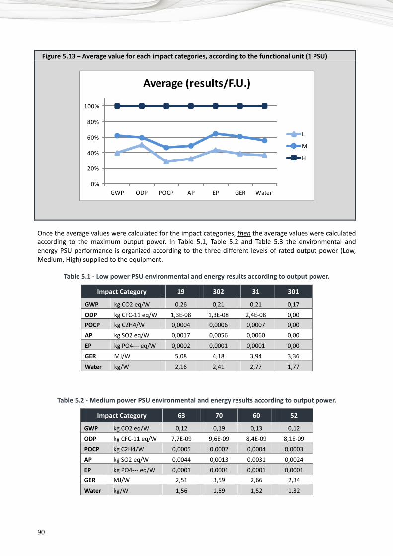
90

Figure 5.13 – Average value for each impact categories, according to the functional unit (1 PSU)

0%

20%

40%

60%

80%

100%

GWP ODP POCP AP EP GER Water

Average (results/F.U.)

L

M

H

Once the average values were calculated for the impact categories, then the average values were calculated according to the maximum output power. In Table 5.1, Table 5.2 and Table 5.3 the environmental and energy PSU performance is organized according to the three different levels of rated output power (Low, Medium, High) supplied to the equipment.

Table 5.1 - Low power PSU environmental and energy results according to output power.

Impact Category 19 302 31 301

GWP kg CO2 eq/W 0,26 0,21 0,21 0,17 ODP kg CFC-11 eq/W 1,3E-08 1,3E-08 2,4E-08 0,00 POCP kg C2H4/W 0,0004 0,0006 0,0007 0,00 AP kg SO2 eq/W 0,0017 0,0056 0,0060 0,00 EP kg PO4--- eq/W 0,0002 0,0001 0,0001 0,00 GER MJ/W 5,08 4,18 3,94 3,36

Water kg/W 2,16 2,41 2,77 1,77

Table 5.2 - Medium power PSU environmental and energy results according to output power.

Impact Category 63 70 60 52

GWP kg CO2 eq/W 0,12 0,19 0,13 0,12 ODP kg CFC-11 eq/W 7,7E-09 9,6E-09 8,4E-09 8,1E-09 POCP kg C2H4/W 0,0005 0,0002 0,0004 0,0003 AP kg SO2 eq/W 0,0044 0,0013 0,0031 0,0024 EP kg PO4--- eq/W 0,0001 0,0001 0,0001 0,0001 GER MJ/W 2,51 3,59 2,66 2,34

Water kg/W 1,56 1,59 1,52 1,32

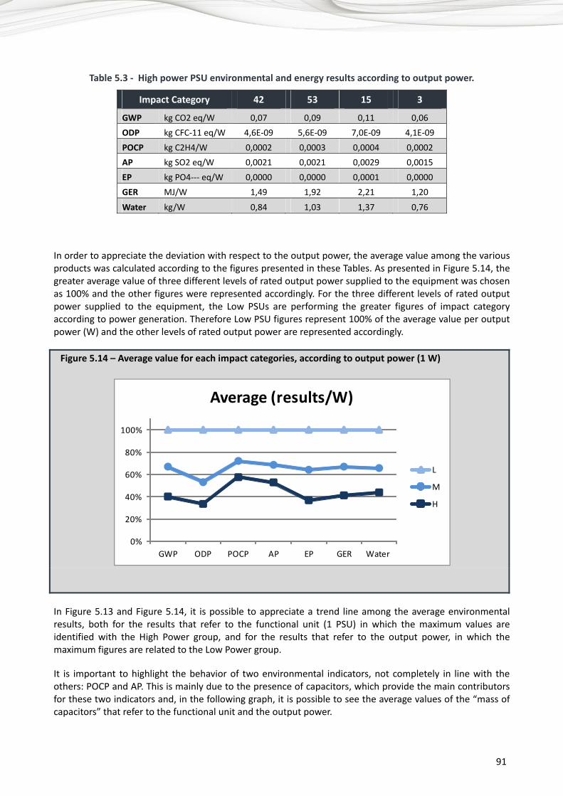
91

Table 5.3 - High power PSU environmental and energy results according to output power.

Impact Category 42 53 15 3

GWP kg CO2 eq/W 0,07 0,09 0,11 0,06 ODP kg CFC-11 eq/W 4,6E-09 5,6E-09 7,0E-09 4,1E-09 POCP kg C2H4/W 0,0002 0,0003 0,0004 0,0002 AP kg SO2 eq/W 0,0021 0,0021 0,0029 0,0015 EP kg PO4--- eq/W 0,0000 0,0000 0,0001 0,0000 GER MJ/W 1,49 1,92 2,21 1,20

Water kg/W 0,84 1,03 1,37 0,76

In order to appreciate the deviation with respect to the output power, the average value among the various products was calculated according to the figures presented in these Tables. As presented in Figure 5.14, the greater average value of three different levels of rated output power supplied to the equipment was chosen as 100% and the other figures were represented accordingly. For the three different levels of rated output power supplied to the equipment, the Low PSUs are performing the greater figures of impact category according to power generation. Therefore Low PSU figures represent 100% of the average value per output power (W) and the other levels of rated output power are represented accordingly.

Figure 5.14 – Average value for each impact categories, according to output power (1 W)

0%

20%

40%

60%

80%

100%

GWP ODP POCP AP EP GER Water

Average (results/W)

L

M

H

In Figure 5.13 and Figure 5.14, it is possible to appreciate a trend line among the average environmental results, both for the results that refer to the functional unit (1 PSU) in which the maximum values are identified with the High Power group, and for the results that refer to the output power, in which the maximum figures are related to the Low Power group.

It is important to highlight the behavior of two environmental indicators, not completely in line with the others: POCP and AP. This is mainly due to the presence of capacitors, which provide the main contributors for these two indicators and, in the following graph, it is possible to see the average values of the “mass of capacitors” that refer to the functional unit and the output power.

92

Figure 5.15 - Presence of capacitors in PSU, referred to the average functional unit and to the average output power, for Low, Medium and High Power PSU.

0%

20%

40%

60%

80%

100%

L M H

Capacitors in PSU (average)

g/F.U.

g/W

5.4.2 Common Power Supply with ETSI specification

Telecom was in charge of a specific study concerning the environmental and energy assessment, fully implementing the Life Cycle Assessment methodology, of a common power supply (identified with device code 44) performing the ETSI specifications.

The considered 44 PSU was a TYPE 2 subcategory b, weighting 92 g, with a nameplate Output Voltage equal to 12 V and a nameplate Output Current equal to 2 A; the rated Output Power was equal to 24 W.

Table 5.4 - 44 PSU component characteristics.

Component unit 44

Case virgin ABS + Recycled ABS g 32,00 Cable g 26,00 Plug & Connectors g 4,00 PCB g 5,00 Transformer g 13,00 Capacitors g 4,00 Inductors g 4,00 Other Electronic Components g 4,00 Total g 92,00

In Table 5.5, it is possible to appreciate the environmental and energy result according to the functional unit (Results/F.U.) and according to power generation (Results/W).

93

Table 5.5 - Type 2 subcategory b, 24W, 44 PSU environmental and energy result according to the functional unit and according to power generation.

Impact category Unit Results/F.U. Results/W

GWP kg CO2 eq 1,54 0,064 ODP kg CFC-11 eq 1,1E-07 4,6E-09 POCP kg C2H4 0,0024 0,00010 AP kg SO2 eq 0,0193 0,00081 EP kg PO4--- eq 0,0011 0,00004 GER MJ 31,6 1,32 Water kg 16,96 0,71

5.4.3 Power generation: a possible comparison

Eventually, the information gathered in Figure 5.13 and in Table 5.5 was organized together as presented in Figure 5.16.

Figure 5.16 - Average value for Low, Medium, High and 44 PSU impact categories, according to the functional unit.

0%

20%

40%

60%

80%

100%

GWP ODP POCP AP EP GER Water

Average (results/F.U.)

L

M

H

44

The information gathered in Figure 5.14 and in Table 5.5 was organized together as presented in Figure 5.17.

94

Figure 5.17 - Average value for Low, Medium, High and 44 PSU impact categories, according to power generation.

0%

20%

40%

60%

80%

100%

GWP ODP POCP AP EP GER Water

Average (results/W)

L

M

H

44

6 Preliminary conclusions

The present study was developed by Politecnico di Torino in order to describe the environmental and energy performance of different PSUs for customer premises equipment, by means of the Life Cycle Thinking approach.

It is important to highlight that the considered PSUs were chosen among an entire population of the products analyzed in the present study in order to provide an overview of the different levels of the rated output power supplied to the equipment (here organized in three levels: Low, Medium and High Power); and within each level of the output power the choice was to select a “sample” composed by a small amount of products with different power outputs. The sample of the considered PSU was chosen according to the possibility of analyzing the influence of different weights, different dimensions and different electronic possibilities according to the apparatus to be powered. The aim was to establish a possible relationship among these characteristics and the environmental and energy performances.

The different power output levels of PSU were analyzed and data coming from the full LCA of a selected common power supply (44 PSUs) were considered for further comparison.

The following conclusions have to be taken into consideration within this specific context of the present study and cannot be used in general terms.

The following preliminary conclusions can be drawn:

• Environmental and energy impacts do not depend only on weight characteristics; the behavior is dependent on the different design choices, especially for electronics, and is at any rate different depending on the single impact category analyzed;

• Environmental and energy impacts do not depend only on output power; in some cases, high power PSU has very similar impacts in comparison to medium power PSUs. The same also applies to the comparison between the medium power and low power category; this demonstrates the importance of adopting accurate design choices (especially for electronics, but also for the plastics) to minimize the environmental burdens associated with the manufacturing phase of the single product;

95

• According to Figure 5.13, it is possible to appreciate an increasing trend of impact for each PSU group among the impact categories considered (higher impacts for High Power PSU); anyway, in Figure 5.14, this trend becomes reversed, if the maximum output power is taken as a reference for the normalization of the environmental results (lower impacts for the maximum output power of High Power PSU);

• In Chapter 5, the LCA interpretation of the environmental results is provided: most of the impacts are due to electronics in all cases; a detailed analysis of the energy efficiency during the use phase should be done in order to understand if the use of advanced electronic components is balanced by a higher efficiency when applied to the final CPE;

• Within the same impact category, it is always possible to identify one example of PSU coupling good use-performance as well as good environmental and energy performances. Depending on the single impact categories, the best in class for the single category can improve the performances of the worst one of a mean percentage around 25-30%, up to 50% in some specific cases. Again, this demonstrates the importance of adopting design rules optimizing the environmental aspects.

A more detailed analysis of the general up-described framework should be necessary in order to assess how environmental impacts depend on the design of electronics as well as on the design of the object (in terms of the material selected).

7 References • Baldo GL, Marino M, Rossi S - Analisi del Ciclo di Vita LCA - Edizioni Ambiente, Milano (2008)

• Boustead I - Boustead Model 5.0, Operating Manual - Boustead Consulting Ltd (2003)

• BSI Specification for the measurement of the embodied greenhouse gas emissions in products and services. PAS 2050, UK, (2008)

• Energy Efficiency and Ecodesign requirements for a common power supply for home gateway, home networking equipment and end devices (HGI)

• EPD Supporting Annex B

• ISO 14025:2006

• ISO 14040:2006

• ISO 14044:2006

• www.ecoinvent.ch

• www.environdec.com

8 Acronyms & Symbols • AP: Acidification Potential

• CED: Cumulative Energy Demand

• EP: Eutrophication Potential

• EPD: Environmental Product Declaration

• ETSI: European Telecommunications Standards Institute

• F.U.: Functional Unit

• GCV: Gross Calorific Value

• GER: Gross Energy Requirement

• GHG: Greenhouse Gases

96

• GWP: Global Warming Potential

• HGI: Home Gateway Initiative

• LCI: Life Cycle Inventory

• LCIA: Life Cycle Impact Assessment

• ODP: Ozone Depletion Potential

• POCP: Photochemical Ozone Creation Potential

• PSU: Power Supply Unit

9 Appendix: Environmental Indicators

9.1 Environmental indicators

The impact categories are calculated by means of the following indicators, in which conversion and characterization factors used for converting LCI data into resource use and potential environmental impacts come from the EPD Regulation Supporting Annex B (www.environdec.com):

• GWP, Global Warming Potential for the time horizon 100 years, is an impact category that groups greenhouse gases (GHG) and calculates their total impact in terms of kg CO2 equivalent, according to the IPCC (Intergovernmental Panel on Climatic Change) reference document, Climate Change 2007; the indicator has been split into: GWP100 Fossil: the contribution of GHG air emission derived by fossil fuel combustion and process; GWP Bio (+): the contribution of GHG air emission derived by biofuel/biomass combustion and

process; GWP Bio (−): the contribu on (credit) of organic carbon embodied in biomass (see Figure 9.1),

excluding packaging;

Figure 9.1 - Differences between GWP Bio and GWP Fossil. Carbon storage may arise during the life-cycle of a product when biogenic carbon forms part or all of a product or when atmospheric carbon is taken up by a product over its life cycle

According to the GHG Protocol Initiative, Product Life Cycle Accounting and Reporting Standard (2010), carbon storage should not be included as a carbon credit in the GHG inventory; however, the carbon storage potential of a product should be reported separately, as identified in the reporting requirements.

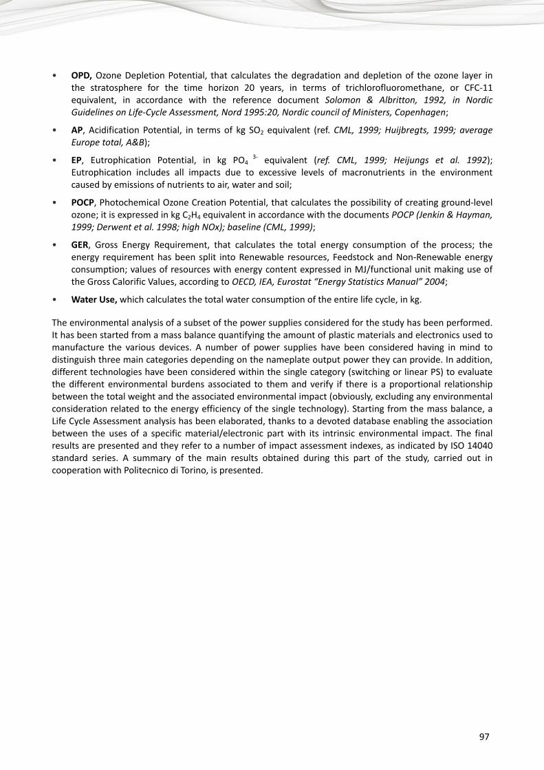
97

• OPD, Ozone Depletion Potential, that calculates the degradation and depletion of the ozone layer in the stratosphere for the time horizon 20 years, in terms of trichlorofluoromethane, or CFC-11 equivalent, in accordance with the reference document Solomon & Albritton, 1992, in Nordic Guidelines on Life-Cycle Assessment, Nord 1995:20, Nordic council of Ministers, Copenhagen;

• AP, Acidification Potential, in terms of kg SO2 equivalent (ref. CML, 1999; Huijbregts, 1999; average Europe total, A&B);

• EP, Eutrophication Potential, in kg PO4 3- equivalent (ref. CML, 1999; Heijungs et al. 1992);

Eutrophication includes all impacts due to excessive levels of macronutrients in the environment caused by emissions of nutrients to air, water and soil;

• POCP, Photochemical Ozone Creation Potential, that calculates the possibility of creating ground-level ozone; it is expressed in kg C2H4 equivalent in accordance with the documents POCP (Jenkin & Hayman, 1999; Derwent et al. 1998; high NOx); baseline (CML, 1999);

• GER, Gross Energy Requirement, that calculates the total energy consumption of the process; the energy requirement has been split into Renewable resources, Feedstock and Non-Renewable energy consumption; values of resources with energy content expressed in MJ/functional unit making use of the Gross Calorific Values, according to OECD, IEA, Eurostat “Energy Statistics Manual” 2004;

• Water Use, which calculates the total water consumption of the entire life cycle, in kg.

The environmental analysis of a subset of the power supplies considered for the study has been performed. It has been started from a mass balance quantifying the amount of plastic materials and electronics used to manufacture the various devices. A number of power supplies have been considered having in mind to distinguish three main categories depending on the nameplate output power they can provide. In addition, different technologies have been considered within the single category (switching or linear PS) to evaluate the different environmental burdens associated to them and verify if there is a proportional relationship between the total weight and the associated environmental impact (obviously, excluding any environmental consideration related to the energy efficiency of the single technology). Starting from the mass balance, a Life Cycle Assessment analysis has been elaborated, thanks to a devoted database enabling the association between the uses of a specific material/electronic part with its intrinsic environmental impact. The final results are presented and they refer to a number of impact assessment indexes, as indicated by ISO 14040 standard series. A summary of the main results obtained during this part of the study, carried out in cooperation with Politecnico di Torino, is presented.

An energy-aware survey on ICT device power supplies

Printed in SwitzerlandGeneva, 2012

Photo credits: Shutterstock®

About ITU-T and Climate Change: itu.int/ITU-T/climatechange/E-mail: greenstandard@itu.int

September 2012!"#"$%&&'()$*+%(,-."/0%1,-*(2-

-------!"#"&*+$,-3*4%1*/%15-

6.789:;7!<-=9>37-;!6=7-=7->9.?8@-

.*+%(*#-7(/"1A6()B"1,)/5-C%(,%1+'&-D%1-!"#"$%&&'()$*+%(,--

About GeSI: www.gesi.orgE-mail: info@gesi.org