An Empirical Study of Time Series Approximation …Department of Computer Science Multimodal...

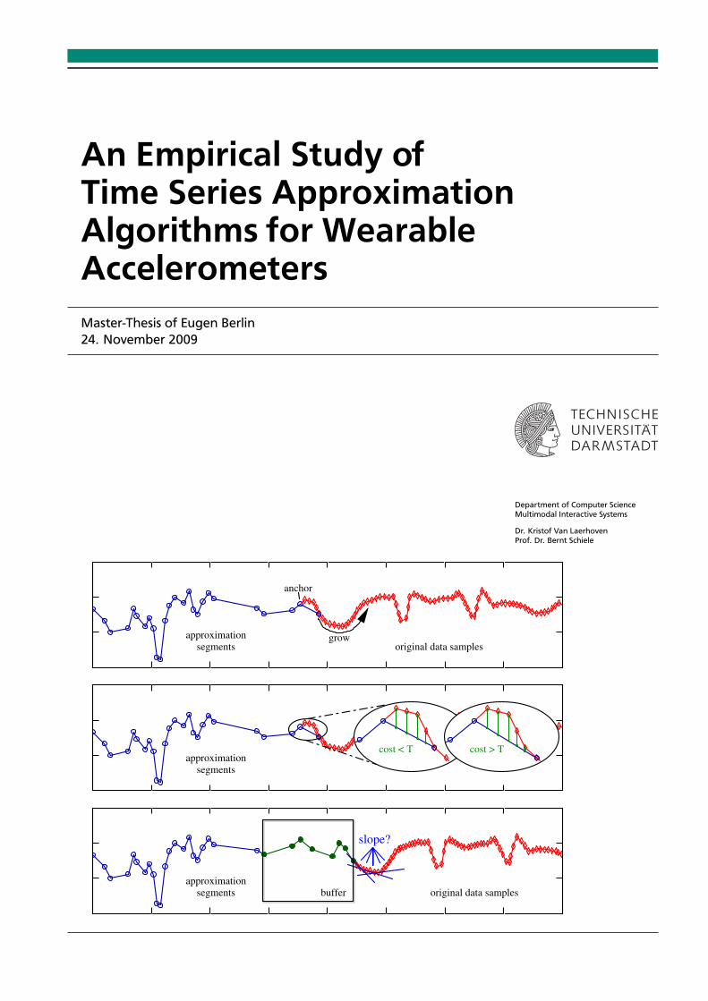
approximation

segments original data samplesbuffer

segments

approximation

segments original data samples

approximation grow

anchor

slope?

cost < T cost > T

An Empirical Study ofTime Series ApproximationAlgorithms for WearableAccelerometersMaster-Thesis of Eugen Berlin24. November 2009

Department of Computer ScienceMultimodal Interactive Systems

Dr. Kristof Van LaerhovenProf. Dr. Bernt Schiele

An Empirical Study ofTime Series Approximation Algorithms for Wearable Accelerometers

vorgelegte Master-Thesis von Eugen Berlin

Tag der Einreichung:

Ehrenwörtliche Erklärung -Declaration of Academic Honesty

Hiermit versichere ich die vorliegendeMaster-Thesis ohne Hilfe Dritter nur mit den angegebenenQuellen und Hilfsmitteln angefertigt zu haben. Alle Stellen, die aus Quellen entnommen wurden,sind als solche kenntlich gemacht. Diese Arbeit hat in gleicher oder ähnlicher Form noch keinerPrüfungsbehörde vorgelegen.

I hereby declare that this Master-Thesis is my own work and has not been submitted in any formfor another degree at any university or other institute. Information derived from the publishedand unpublished work of others has been acknowledged in the text and a list of references isgiven in the bibliography.

Darmstadt, 24.11.2009

(Eugen Berlin)

i

ii Ehrenwörtliche Erklärung -Declaration of Academic Honesty

Zusammenfassung

Die Aktigraphie ist ein großes Forschungsgebiet, das auf die Erkennung bzw. die Vorhersagevon Aktivitäten und Handlungen einer Person nur auf Grundlage von einzelnen Gesten und Be-wegungen abzielt. Da dieses mit Standardhardware erreicht werden kann, wie zum Beispieldurch den Einsatz von Kameras in der jeweiligen Umgebung oder durch die am Körper ge-tragene Beschleunigungssensoren, liegt der Fokus der Forschung auf der Mustererkennungund den Algorithmen für Maschinelles Lernen, die die Körperhaltung oder Bewegungsmuster(Zurückschwingen des Arms) erkennen und dabei die markanten Merkmale für bestimmte Ak-tivitäten (Tennis spielen) erlernen. Unsere Arbeit erforscht die unterste Ebene des Forschungs-gebiets, wo Bewegungsmuster charakterisiert und mit den schon verfügbaren Beispielmusternverglichen werden.

Der erste Teil dieser Arbeit zielte ab auf präzise und effiziente Approximationsalgorithmenfür die Charakterisierung von Bewegungsmustern in den Beschleunigungsdaten eines tragbarenBeschleunigungssensors. Dieser Teil umfasste die Implementation von Standardalgorithmen,wie zum Beispiel der grundlegenden statistischen Kennzahlen oder der schnellen Fourier Trans-formation, aber auch der jüngsten wissenschaftlichen Erkenntnisse, wie SwiftSegs von Sick etal. Unser Beitrag in diesem Forschungsgebiet ist eine Modifikation des SWAB Algorithmus unddie Ergebnisse der dazugehörigen Experimente, die zeigen, dass unsere Modifikation schnellerist als SWAB und dabei die Beschleunigungsdaten genau so gut approximiert.

Der zweite Teil der Studie beschäftigt sich mit drei Algorithmen für Mustervergleiche fürgenau solche Bewegungsmuster: Dynamic Time Warping, die k längsten Segmente, und Inter-polation wurden auf zwei Datensätzen evaluiert. Dabei wurden die Algorithmen hinsichtlichder Güte der Klassifikationsergebnisse als auch der Geschwindigkeit verglichen. Die Ergebnisseder Evaluation zeigen, dass die Verwendung von Dynamic Time Warping bessere Klassifikation-sergebnisse liefert, die beiden anderen Algorithmen jedoch sehr viel schneller sind. Jedocherzielt man auch mit diesen zwei Algorithmen und mit Bedacht gewählten Parametern sowieder Grös̈s e des Query-Fensters durchaus vergleichbare Ergebnisse.

Diese Arbeit schließt mit einigen Vorschlägen und dem Ausblick für zukünftige Forschungsar-beiten, die während dieser Studie als viel versprechend erkannt wurden.

iii

iv Zusammenfassung

Abstract

Activity recognition is a large field of research where the aim is to predict a user’s actions throughhis or her physical gestures and motions. As this can be achieved with standard hardware, suchas cameras in the environment or on-body inertial sensors, the focus of this research is largelyon pattern recognition and machine learning algorithms that detect poses and motions patterns(such as a backhand swing) and learn which are tell-tale signs for activities (such as tennis). Thisthesis investigates the lower level part of this research where motion patterns are characterizedand matched to previously seen examples.

A first set of investigations has targeted accurate and efficient approximation algorithms forcharacterizing motion patterns within wearable accelerometer data. This involved implement-ing standard algorithms such as basic statistics and fast Fourier transform, but also very recentwork such as Sick et al.’s SwiftSegs. We contribute in this field with a modification of theSWAB algorithm, complemented with experiments that show it is faster and approximates anaccelerometer signal as well as SWAB.

A second study has involved three matching algorithms for these motion patterns: dynamictime warping, k longest segments, and interpolation matching were evaluated on two datasetsin order to detect which ones outperform the others in a classification setting and in matchingspeed. Results show that matching with dynamic time warping results in better classificationperformance, but the two other algorithms are much faster and, given well-chosen parametersand in particular the pattern’s window width, obtain comparable results.

The thesis is concluded with a set of recommendations and outlook for future work that thisresearch has revealed to be promising.

v

vi Abstract

Thesis Task Description

Introduction

Wearable accelerometers have become increasingly embedded in personal devices such as mo-bile phones, laptops, and wristwatches, due to their low-power MEMS design and easy-to-interpret sensor data. Most applications on these devices use in particular the accelerometer’soutput as a way to measure tilt and posture in a relatively cheap way, while filtering out the mo-tion characteristics. Research has since more than a decade recognized the significance of themotion patterns exhibited by the acceleration sensor, leading to detection of characteristic move-ments for a number of applications. One of these applications is the detection of short gesturesmade by the wearer of a wrist-worn accelerometer, allowing a variety of complex computinginterfaces and implicit interaction.

This thesis will examine the foundations of this field by comparing the most promising algo-rithms, available from time series mining, to represent short motion patterns in accelerometerdata. The challenge here is to do this in the most optimal way for later visual inspection andautomated classification. As such, the goal is to find the superior approach in both modellingthe essence of the gesture, while also requiring the approach to be embeddable in low-powersystems.

Task Description

1. The student will start with familiarizing himself with time series representation, and in par-ticular recent scientific publications on algorithms that approximate time series segments[1]. Starting points will be recent improved heuristics based on Dynamic Time Warping[2], Piecewise Polynomial Approximation, and Symbolic String Approximations [3].

2. The main contribution of the thesis will be in the form of an off-line experiment usingrealistic data. A comparison between promising candidate algorithms derived from theprevious step will then be done using a data-driven experiment. These algorithms convertraw data into a time series’ approximation.

• For this, a prototypical implementation of these algorithms needs to be written andtested first. Language of choice is Matlab.

• As an inherent requirement for the selection of algorithms, it is important to restrictthe choices to heuristics that are online and have low time complexity. This is basedupon the need for the algorithm to be implementable on low-power (wearable) plat-forms.

• The algorithms will be tested on wearable accelerometer data, available from MIS’repository (i.e., no additional data logging is required).

• The evaluation will be based upon precision-recall measurements from classificationof the time series’ approximations with basic nearest neighbour selection.

vii

3. As a final task, the algorithm(s) that come(s) out as the most promising from the previousstep, will be implemented on a microcontroller-based wearable sensing platform. The pur-pose of this task is a feasibility study, which includes measurements of efficiency (indicatedby power consumption) and a comparison to a standard approach using logging of averageand standard deviation.

Environment

Matlab and C/C++ will be used for the prototyping of the algorithms, while CCS C is envisionedfor the implementation in the end-phase of the thesis.

[1] Keogh, Chu, Hart, and Pazzani. An online algorithm for segmenting time series. In IEEEInternational Conference on Data Mining, pages 289–296, 2001.[2] Rabiner and Juang. Fundamentals of speech recognition. Prentice-Hall, Inc., 1993[3] Lin, Keogh, Wei, and Lonardi. Experiencing SAX: a novel symbolic representation of timeseries. DMKD Journal, 2007.

viii Thesis Task Description

Contents

1 Introduction 11.1 Activity recognition . . . . . . . . . . . . . . . . . . . . . . . . . . . . . . . . . . . . . . . 11.2 Long-term activity recognition and wearable accelerometers . . . . . . . . . . . . . 21.3 Annotations in activity recognition . . . . . . . . . . . . . . . . . . . . . . . . . . . . . 2

2 Related Work 5

3 Approximation Algorithms 73.1 Traditional Features . . . . . . . . . . . . . . . . . . . . . . . . . . . . . . . . . . . . . . . 7

3.1.1 Mean and Variance . . . . . . . . . . . . . . . . . . . . . . . . . . . . . . . . . . . 73.1.2 Discrete Fourier Transformation . . . . . . . . . . . . . . . . . . . . . . . . . . . 8

3.2 Piecewise Linear Approximation . . . . . . . . . . . . . . . . . . . . . . . . . . . . . . . 93.2.1 Sliding Window . . . . . . . . . . . . . . . . . . . . . . . . . . . . . . . . . . . . 103.2.2 Bottom-Up . . . . . . . . . . . . . . . . . . . . . . . . . . . . . . . . . . . . . . . . 113.2.3 SWAB: Sliding Window and Bottom-Up . . . . . . . . . . . . . . . . . . . . . . 133.2.4 mSWAB: modified SWAB . . . . . . . . . . . . . . . . . . . . . . . . . . . . . . . 14

3.3 Piecewise Polynomial Approximation . . . . . . . . . . . . . . . . . . . . . . . . . . . . 16

4 Matching Algorithms 194.1 Dynamic Time Warping . . . . . . . . . . . . . . . . . . . . . . . . . . . . . . . . . . . . 194.2 K Longest Segments . . . . . . . . . . . . . . . . . . . . . . . . . . . . . . . . . . . . . . 204.3 Interpolation . . . . . . . . . . . . . . . . . . . . . . . . . . . . . . . . . . . . . . . . . . . 21

5 Evaluation Methods 235.1 Approximation . . . . . . . . . . . . . . . . . . . . . . . . . . . . . . . . . . . . . . . . . . 235.2 Matching and Classification . . . . . . . . . . . . . . . . . . . . . . . . . . . . . . . . . . 24

5.2.1 Methodology . . . . . . . . . . . . . . . . . . . . . . . . . . . . . . . . . . . . . . 255.2.2 Generic Evaluation Script . . . . . . . . . . . . . . . . . . . . . . . . . . . . . . 25

6 Experiments and Results 316.1 Approximation . . . . . . . . . . . . . . . . . . . . . . . . . . . . . . . . . . . . . . . . . . 31

6.1.1 Initial Test - Runtime . . . . . . . . . . . . . . . . . . . . . . . . . . . . . . . . . 316.1.2 Extended Test - Accuracy, Runtime, Footprint . . . . . . . . . . . . . . . . . . 32

6.2 Matching and Classification . . . . . . . . . . . . . . . . . . . . . . . . . . . . . . . . . . 346.2.1 Initial Matching Experiments . . . . . . . . . . . . . . . . . . . . . . . . . . . . 346.2.2 Extended Matching Experiments . . . . . . . . . . . . . . . . . . . . . . . . . . 36

7 Conclusions and Future Work 417.1 Summary and Conclusion . . . . . . . . . . . . . . . . . . . . . . . . . . . . . . . . . . . 417.2 Future Work . . . . . . . . . . . . . . . . . . . . . . . . . . . . . . . . . . . . . . . . . . . 42

ix

Bibliography 43

A Experiment Results 45

B Time Series GUI and X11 Plots 59

x Contents

List of Figures

3.1 Mean and Variance vs. DFT . . . . . . . . . . . . . . . . . . . . . . . . . . . . . . . . . . 83.2 Sliding Window . . . . . . . . . . . . . . . . . . . . . . . . . . . . . . . . . . . . . . . . . 103.3 Mean and Variance vs. DFT vs. Sliding Window . . . . . . . . . . . . . . . . . . . . . 113.4 Bottom-Up . . . . . . . . . . . . . . . . . . . . . . . . . . . . . . . . . . . . . . . . . . . . 123.5 SWAB: Sliding Window and Bottom-Up . . . . . . . . . . . . . . . . . . . . . . . . . . 133.6 SWAB timings . . . . . . . . . . . . . . . . . . . . . . . . . . . . . . . . . . . . . . . . . . 143.7 mSWAB: modified SWAB . . . . . . . . . . . . . . . . . . . . . . . . . . . . . . . . . . . 153.8 Polynomial Approximation . . . . . . . . . . . . . . . . . . . . . . . . . . . . . . . . . . 173.9 Polynomial Approximation – Sliding and Growing Windows approach . . . . . . . 18

4.1 Matching: Dynamic Time Warping . . . . . . . . . . . . . . . . . . . . . . . . . . . . . . 194.2 Matching: K longest segments . . . . . . . . . . . . . . . . . . . . . . . . . . . . . . . . 214.3 Matching: Interpolation . . . . . . . . . . . . . . . . . . . . . . . . . . . . . . . . . . . . 214.4 Matching: Interpolation Issue . . . . . . . . . . . . . . . . . . . . . . . . . . . . . . . . . 22

5.1 Script Description 1 . . . . . . . . . . . . . . . . . . . . . . . . . . . . . . . . . . . . . . . 265.2 Script Description 2 . . . . . . . . . . . . . . . . . . . . . . . . . . . . . . . . . . . . . . . 265.3 Script Description 3 . . . . . . . . . . . . . . . . . . . . . . . . . . . . . . . . . . . . . . . 275.4 Scores Plot . . . . . . . . . . . . . . . . . . . . . . . . . . . . . . . . . . . . . . . . . . . . 275.5 Script Description 4 . . . . . . . . . . . . . . . . . . . . . . . . . . . . . . . . . . . . . . . 285.6 Script Description: Final Overview . . . . . . . . . . . . . . . . . . . . . . . . . . . . . 29

6.1 Evaluation of Approximation Algorithms . . . . . . . . . . . . . . . . . . . . . . . . . . 336.2 Walk8 experiment setup . . . . . . . . . . . . . . . . . . . . . . . . . . . . . . . . . . . . 346.3 Walk8 matching results . . . . . . . . . . . . . . . . . . . . . . . . . . . . . . . . . . . . 356.4 Extended Matching - DTW accuracies in comparison . . . . . . . . . . . . . . . . . . 376.5 Extended Matching - DTW best accuracy result . . . . . . . . . . . . . . . . . . . . . . 38

A.1 Walk8 - accuracy plot - mSWAB_05_80_DTWCS_15 . . . . . . . . . . . . . . . . . . . 46A.2 Walk8 - best result - w200_mSWAB_05_80_DTWSC_15 . . . . . . . . . . . . . . . . 46A.3 Walk8 - accuracy plot - mSWAB_05_80_KLS_05 . . . . . . . . . . . . . . . . . . . . . 47A.4 Walk8 - best result - w100_mSWAB_05_80_KLS_05 . . . . . . . . . . . . . . . . . . . 47A.5 Walk8 - accuracy plot - mSWAB_05_80_KLS_10 . . . . . . . . . . . . . . . . . . . . . 48A.6 Walk8 - best result - w150_mSWAB_05_80_KLS_10 . . . . . . . . . . . . . . . . . . . 48A.7 Walk8 - accuracy plot - mSWAB_05_80_KLS_15 . . . . . . . . . . . . . . . . . . . . . 49A.8 Walk8 - best result - w150_mSWAB_05_80_KLS_15 . . . . . . . . . . . . . . . . . . . 49A.9 Walk8 - accuracy plot - mSWAB_05_80_IP_10 . . . . . . . . . . . . . . . . . . . . . . 50A.10 Walk8 - best result - w300_mSWAB_05_80_IP_10 . . . . . . . . . . . . . . . . . . . . 50A.11 Walk8 - accuracy plot - mSWAB_05_80_IP_20 . . . . . . . . . . . . . . . . . . . . . . 51A.12 Walk8 - best result - w300_mSWAB_05_80_IP_20 . . . . . . . . . . . . . . . . . . . . 51A.13 Walk8 - accuracy plot - mSWAB_10_80_DTWCS_15 . . . . . . . . . . . . . . . . . . . 52

xi

A.14 Walk8 - best result - w300_mSWAB_10_80_DTWSC_15 . . . . . . . . . . . . . . . . 52A.15 Walk8 - accuracy plot - mSWAB_10_80_KLS_05 . . . . . . . . . . . . . . . . . . . . . 53A.16 Walk8 - best result - w150_mSWAB_10_80_KLS_05 . . . . . . . . . . . . . . . . . . . 53A.17 Walk8 - accuracy plot - mSWAB_10_80_KLS_10 . . . . . . . . . . . . . . . . . . . . . 54A.18 Walk8 - best result - w150_mSWAB_10_80_KLS_10 . . . . . . . . . . . . . . . . . . . 54A.19 Walk8 - accuracy plot - mSWAB_10_80_KLS_15 . . . . . . . . . . . . . . . . . . . . . 55A.20 Walk8 - best result - w150_mSWAB_10_80_KLS_15 . . . . . . . . . . . . . . . . . . . 55A.21 Hapkido - accuracy plot - mSWAB_05_80_DTWSC_15 . . . . . . . . . . . . . . . . . 56A.22 Hapkido - best result - Hapkido_w300_mSWAB_05_80_DTWSC_15 . . . . . . . . . 56A.23 Hapkido - accuracy plot - mSWAB_10_80_DTWSC_15 . . . . . . . . . . . . . . . . . 57A.24 Hapkido - best result - Hapkido_w300_mSWAB_10_80_DTWSC_15 . . . . . . . . . 57

B.1 GUI for approximation and matching algorithms . . . . . . . . . . . . . . . . . . . . . 59

xii List of Figures

List of Tables

6.1 Comparing execution time of various approximation algorithms . . . . . . . . . . . 326.2 Comparing accuracy and execution time of DTW and KLS . . . . . . . . . . . . . . . 36

xiii

xiv List of Tables

1 Introduction

This chapter will introduce the basic concept of activity recognition, and the specific scope wewill follow in this thesis towards achieving activity recognition for a wearable inertial sensorsetting. In particular, the sensor type we will restrict ourselves to is the accelerometer; a moti-vation for this choice will be given in a dedicated section as well that discusses the differenceswhen recording activities over long periods of time. A next section will specifically introduce so-lutions so far presented in the annotation by the user of their activities, i.e., how the system canlink activity data to the actual semantics. A discussion of several of the directions that previousresearch has taken in this area will follow this chapter.

1.1 Activity recognition

The definition of activity recognition can be loosely defined as the recognition of an agent’sactions and goals, by means of algorithms using previously observed actions with sensors eitherattached to the agent or in its vicinity. The use of the name agent in this definition is intended toinclude also the recognition of activities from robots or software agents, but most often humanactivities are intended. The choice of what type of activities, whether they can be overlappingor not (e.g., “eating” and “watching tv”), or have hierarchies (e.g., “running” and “playingfootball”) or reside on just one layer, makes activity recognition is large domain where manyapplications have been suggested and many methods have been devised for estimating activities.

The field of activity recognition is a vast research domain spanning several disciplines, fromcomputer science and engineering sciences such as machine learning, computer vision, embed-ded systems design, and distributed systems, but also including disciplines from the humanitiessuch as psychology or ethnography. The sensors that are used for activity recognition may bedivided in those that are relying on sensors on the body of the person, where usually inertialsensors are used to characterize activities with certain motions or location technologies deriveactivity from location, and environmental sensors such as cameras linking sequences of bodypostures to activities or tracker systems.

Activity recognition has been proposed for a multitude of applications. For instance, as partof a system that automates the monitoring of elderly patients to assess their independence (alsocalled Assisted Living) by checking whether certain activities are still carried out, or for improv-ing memory by automatically filling in a searchable diary with activity information. Anotherexample from the medical domain is the monitoring of psychiatric patients for whom activities,the way they are carried out and their frequency and intensity is vital; such patients would in-clude those with depressions and bipolar disorders. Several applications for activity recognitionhave also been suggested for the training of knowledge workers and maintenance engineers,where the activities are very task-oriented and their succession and execution are visualized ortrigger appropriate computer tasks (such as showing the correct page in a maintenance manualin the engineer’s wearable display). Less critical applications mention the usage of recognizedactivities for fitness training or for conveying status messages on instant messengers.

1

1.2 Long-term activity recognition and wearable accelerometers

Long-term activity recognition relies on wearable sensors that log the physical actions of thewearer, so that these can be analyzed afterwards. Recent progress in sensor technologies (es-pecially MEMS technology) and embedded and integrated circuits has made it feasible to loghigh-resolution inertial data on small devices, resulting in increasingly large data sets. Althoughgyroscopes and magnetometers have been used thoroughly as well for inertial sensing of ac-tivities, the output from 3D accelerometer is particularly well-suited for longer recordings asthey are of low dimension and complexity. Adding these other types of inertial sensors wouldmean producing a larger and more power-hungry logging device of a higher complexity. Restric-tion to a 3D accelerometer means less information, especially in 3D orientation, but as it is farless complex to build both embedded hardware and software for them we restrict ourselves tothis modality alone. A choice has thus been made for longer recordings with a smaller simplersensor, at the cost of losing turning and compass information.

This thesis focuses on this type of longer logging of inertial data, where test subjects areexpected to wear a sensor for a period of time spanning at least several days and lasting weeks oreven months. The subjects then need to upload their logged accelerometer data to a computer,so that the recordings can be analyzed by both algorithms and the users themselves. Apart fromthe visualization of this data, the annotation of the data coming initially from sensor values issignificant.

1.3 Annotations in activity recognition

Several methods have been suggested for the annotation of wearable data. The three most-usedmethods are called time diary, experience sampling, and self-recall. The latter has been foundto be especially promising in longer-running trials as subjects doing the annotation can choosethemselves when to initiate this, as well as how long and detailed to do this. For this reason,we focus on off-line methods that can be performed on a desktop machine using downloadedactivity data. It is important to remark here that self-recall can in this case also include visual-izations from the uploaded data, helping the user in finding relevant or surprising sections inthe data for annotation.

We expect the participating users to work with raw data, or at least close approximationsthereof, analysing it without high level abstractions such as activity labels. Since the subjectsand also the computer are confronted with large data sets, algorithms for properly and memory-efficiently approximating the raw data are essential. The user is to be provided with a visualrepresentation of the data, which as we will see in a later chapter, will reduce the number ofapproximation algorithms to those that not only approximate the raw data as good as possible,but allow easy and straight-forward visualisation of the approximation. Test subjects then willbe able to work with the visual representation of the approximation of the raw data. Zooming inand out on the data set will allow the subject to search for short and interesting motion patternsand annotate these. Also, matching algorithms shall support the user in providing close matchesto a selected pattern, thus easing and speeding up the annotation phase. Since matching hast tobe conducted on large data sets, the algorithms need to be fast and not time consuming on theone hand, and give good accuracy on the other. This is, as we will see, a significant trade-off tobe made.

2 1 Introduction

The remainder of this thesis is structured as follows: First we will take a look at related workto set our work in context of the scientific research. The third chapter will present variousapproximation algorithms, starting with traditional features, then focusing on piecewise linearapproximation and afterwards shortly presenting polynomial approximations. The fourth chap-ter will present and discuss the three mentioned matching algorithms. In chapter five we willfocus on the evaluation methods that have been used to evaluate and benchmark the perfor-mance of the presented algorithms, paying a lot of attention to the N-fold cross-validation andnearest-neighbor classification as well as the generic evaluation script. Experiments and resultswill be presented in chapther six. The thesis closes with conclusions and outlook on future work.

1.3 Annotations in activity recognition 3

4 1 Introduction

2 Related Work

Approximation of human activity data

Previous studies have applied a large variety of approximations and features to accelerome-ter data. Among the more prominent are (constant segments of) mean and variance, as wellas Fourier coefficients, wavelet matches [22], and several approaches applying conversion insequences of symbols.

The appeal of using the mean and variance over a sliding window as features for accelerationis particularly high because of their efficient implementation. The mean tends to capture thelocal posture of the body, and variance describes how much motion is present in the signal.The mean and variance together have also been used with much success in detecting high-levelactivities by calculating them over large sliding windows [6]. These features have been usedeffectively when combining multiple body-worn sensors [20] or in short sliding windows withan HMM-based approach [28].

Several features are in contrast more costly to calculate but have resulted in better perfor-mance. Autocorrelation, Discrete Fourier Transform, and filterbank analysis can be expectedto work especially well on activities with dominant frequencies, and have been identified assuperior in several comparison studies (e.g., [7]).

Other approaches quantize the data in strings of symbols and look for sequences in this data.Minnen et al. [19] proposed to discretize the inertial time series data first by fitting K Gaussiansto achieve a roughly equal distribution of symbols, after which repetitive sub-sequences in thedata, so-called motifs, are searched for. These motifs then train HMMs to allow unsupervisedlearning of activities. Later work used the symbolic aggregate approximation (SAX [16]) algo-rithm as a way to represent the time series. The authors of the latter have recently introducediSAX [25].

Apart from [1], where the authors use the SWAB algorithm on fused acceleration and gy-roscope data to detect relevant gestures made by the wearer of the sensor, piecewise linearapproximation of wearable inertial data has thus far not often been explored.

Work on matching has thus far used mostly Euclidean distance over features or dynamictime warping (DTW) [5] to compare subsequences in inertial sensor data, or window basedclassification, gesture spotting [20], or motif discovery [19].

Activity Recognition and Long-Term Activity recognition

Due to rapid developmental progresses in computer technology, hardware has become smallerand less power consuming. On account of this, it has become easier to gather activity data overlonger periods of time. We discuss three examples out of a large body of scientific publicationstargeting activity recognition in particular to give a glance on the data used and progress inrecording longer data sets.

The work by Lukowicz et al. [18] data is recorded for several minutes only, but the data isgathered by a body network of sensors. As the overall aim of the authors is to provide reliable

5

context recognition in every-day work situations, the experiments consist of recognizing sev-eral tasks such as hammering or sawing in a wood workshop ten times by one person. Data isrecorded using a network combining two microphones (located at the subject’s right hand andchest) and three accelerometers (located at the wrists and upper right arm). For experiments,the authors labeled the data by hand, and performed recognition of activities by sound usinga Fast Fourier Transformation (FFT) to obtain spectral components, which had their dimensionreduced by Linear Discriminant Analysis(LDA). To further improve the method LDA was com-bined with Intensity Analysis (IA) which exploits differences in intensity of the two microphonesto preselect the segments. For classifying activities using accelerometer data, the authors usedhidden Markov models (HMMs). The reported overall accuracy reached was 83.5% includingzero false positives. Short-term experiments as this work have the advantage that the groundtruth is reliably obtained due to direct observations as the data is recorded. Collecting data fromseveral body locations might be too intricate for long-term deployment as well, but gives a lotmore information than a single sensor.

As an example of a bigger data set, Lester et al. [15] recorded several hours of data from 12individuals spread over several days. The objective of this work is to develop a personal activityrecognition system which is worn at a single body location, is cost effective, and works out ofthe box for different users, resulting in activities such as sitting, walking, riding an elevator orbrushing teeth. To record the data they used a multi-modal sensor board (MSB), a powerfulsensor holding seven different sensors (microphone, phototransistor, accelerometer, compass,barometer and temperature sensor, ambient light sensor, humidity and temperature sensor)connected to an Intel Mote. Out of the sensor data, 651 features are computed (includingmean, variance, and FFT coefficients). The authors used a customized activity classificationalgorithm combining boosting, utilizing a set of weak classifiers to preselect useful features, witha layer of hidden Markov models which perform the classification. The ground truth data wereobtained by observers who annotated the data in real time while it was recorded. The threemost important sensors were found to be the accelerometer, audio and barometric pressuresensors. The overall accuracy was found to be about 90%. On the other hand, using onlythe accelerometers the accuracy dropped to 65%. This work shows that everyday usability ofactivity recognition systems can be solved and that it is possible to deploy low cost sensors in asingle device which can be carried on the body.

One of the biggest (especially longest) data sets available to date is one of 10 weeks of databy Logan et al. [17]. This study monitored a married couple living in a highly instrumentedliving environment called PlaceLab, where over 900 sensors of different types (e.g. wired reedswitches, current and water flow inputs, motion detectors, or RFID tags) are spread over theapartment. In addition, the male subject wore accelerometers on wrist and waist and an RFIDreader bracelet. During the 10 weeks of monitoring the authors obtained 15 days of labeleddata annotated by a third party. The annotated activities (43 in the data set 98 in total) belongto normal everyday life, such as using a computer, sleeping, cooking, drying dishes or watchingTV. The aim of this study was to compare the different sensor types for activity recognitionin an as realistic as possible way, avoiding any type of bias. The results of the study showedthat environmental location sensors outperformed body worn accelerometers and RFID tags foralmost every activity, due to most activities being performed in special locations (e.g., doing thedishes in the kitchen area). This work was a huge feat since the ground truth was obtainedthrough audio and video observation and annotations by a third party, which proved to beaccurate and unbiased, but also very expensive.

6 2 Related Work

3 Approximation Algorithms

In this chapter we will be looking at different approaches to approximate raw human accelerom-eter data. The requirements for the approximation algorithm specified in the introduction arethe basis for the following selection and evaluation. We will start by looking at the algorithmsfrom a theoretical point of view. The evaluation of the algorithms can be found in chapter 6.

3.1 Traditional Features

Traditional features like mean and variance, as well as Discrete Fourier Transformation, havebeen widely used throughout scientific work [7]. Thus, this is the main reason these approx-imation approaches will be looked at in first place. Unfortunately, traditional features do notalways qualify for our demands of precise description of motion patterns, as we will see in thefollowing section.

3.1.1 Mean and Variance

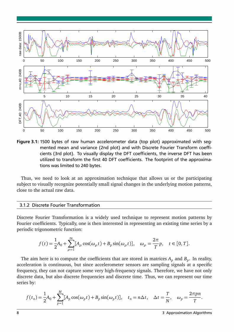
A very common approach to represent motion patterns is by calculating the mean and variancevalues per signal dimension (for human motion patterns this is in our case accelerometer axis)over a sliding window. The mean over human-worn acceleration sensors tends to capture thelocal posture of the body, while the variance describes how much motion is present in thesignal. Both mean and variance together have been used with much success in detecting high-level activities by calculating them over large sliding windows of 4 seconds to up to 8 minutes[6].

The implementation of this approximation approach is efficient and fast especially since lan-guages and libraries (such as Matlab) have built-in implementations. On the other hand, thevisual representation of the resulting approximation is not straight-forward. A common visualrepresentation of what is encoded in mean and variance, is to use segmented mean valuesenriched with y-bars for variance (Figure 3.1, plot 2).

Since we are searching for an approach that not only approximates the raw accelerometerdata for computational or matching purposes, but whose resulting approximation can easily bevisualized and also visually represents the raw data closely, we must conclude that mean andvariance are not as human readable as motion features could be.

To make this more clear, let us have a look at a small example. As can be seen in Figure 3.1,there is a sharp peak in raw accelerometer data at t ≈ 170. The approximation delivered bymean and variance reflects the high accelerations (high variance represented by the y-bars), butdoes not show the motion pattern itself. For example, when confronted with approximationof the raw data only, a human will actually not be able to visually differentiate between fastup-down-up or down-up-down arm motions.

7

0 50 100 150 200 250 300 350 400 450 500

raw

dat

a: 1

500B

5 10 15 20 25 30 35 40

m+

v,40

: 240

B

0 50 100 150 200 250 300 350 400 450 500

DF

T,4

0: 2

40B

Figure 3.1: 1500 bytes of raw human accelerometer data (top plot) approximated with seg-mented mean and variance (2nd plot) and with Discrete Fourier Transform coeffi-cients (3rd plot). To visually display the DFT coefficients, the inverse DFT has beenutilized to transform the first 40 DFT coefficients. The footprint of the approxima-tions was limited to 240 bytes.

Thus, we need to look at an approximation technique that allows us or the participatingsubject to visually recognize potentially small signal changes in the underlying motion patterns,close to the actual raw data.

3.1.2 Discrete Fourier Transformation

Discrete Fourier Transformation is a widely used technique to represent motion patterns byFourier coefficients. Typically, one is then interested in representing an existing time series by aperiodic trigonometric function:

f (t) =1

2A0+

∞∑

ρ=1

[Aρ cos(ωρ t) + Bp sin(ωρ t)], ωρ =2π

Tp, t ∈ [0, T].

The aim here is to compute the coefficients that are stored in matrices Ap and Bp. In reality,acceleration is continuous, but since accelerometer sensors are sampling signals at a specificfrequency, they can not capture some very high-frequency signals. Therefore, we have not onlydiscrete data, but also discrete frequencies and discrete time. Thus, we can represent our timeseries by:

f (tn) =1

2A0+

M∑

p=1

[Ap cos(ωp t) + Bp sin(ωp t)], tn = n∆t, ∆t =T

N, ωp =

2πpn

T.

8 3 Approximation Algorithms

Here, we need to determine M and the coefficient matrices. When sampling N data values, wecan determine N unknown coefficients: A0, A1, . . . , AN/2 and B1, B2, . . . , BN/2−1. Hence we can setM = N/2. Also, we include B0 and BN/2 for symmetry reasons, but since the corresponding sinefunction factors evaluate to zero, these two coefficients can have random values. For simplicitywe set them to zero: B0 = BN/2 = 0. Finally, the coefficient matrices Ap and Bp are computedusing the following formulas:

Ap =2

N

N∑

n=1

y(tn) cos(2πpn

N), p = 1,2, . . . , N/2− 1

Bp =2

N

N∑

n=1

y(tn) sin(2πpn

N), p = 1,2, . . . , N/2− 1

A0 =1

N

N∑

n=1

y(tn) and AN/2 =1

N

N∑

n=1

y(tn) cos(nπ)

Besides the computational complexity of this approach, the approximation also needs to bevisualized. To accomplish this, an inverse DFT is needed to compute and plot the graphs fromthe previously computed coefficient matrices (Figure 3.1, plot 3). This additional computationadds to the time needed for overall approximation and visualization.

Since this approximation and visualization approach is not online and not as fast and straight-forward as one might like to have for human accelerometer data, other approximation tech-niques will be considered in the next section.

3.2 Piecewise Linear Approximation

Because of the less optimal visualization of the approximation results delivered by both meanand variance as well as Discrete Fourier Transform, other approximation approaches have beenstudied. Popular from the data mining community, Piecewise Linear Approximation (PLA) lendsitself to be looked at more closely, since ...

We will start with Sliding Window, a common representative of PLA algorithms, and show whythis is a promising approach. Then, we will be looking at the Bottom-Up algorithm, followed bythe SWAB approach. Finally, a small modification of the original SWAB algorithm, mSWAB, willbe presented as a faster alternative for accelerometer data.

Key to all PLA approaches is the approximation of a time series (in our case – continuoushuman acceleration data) into a representation of linear segments that is efficient to manipulateand faster to process than the raw sensor data. The linear segments can be visualized in anidentical way to the original data in a time series plot, while the number of data points issignificantly reduced without losing the intrinsic nature of the underlying activity. All thoseapproaches have one thing in common: deviation from the raw data is only allowed up to aspecific user-defined cost threshold.

3.2 Piecewise Linear Approximation 9

segments original data samplesapproximation grow

anchor

segmentsapproximation

cost < T cost > T

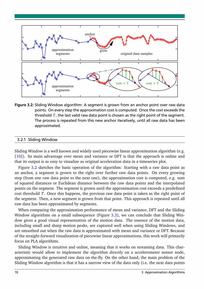
Figure 3.2: Sliding Window algorithm: A segment is grown from an anchor point over raw datapoints. On every step the approximation cost is computed. Once the cost exceeds thethreshold T , the last valid raw data point is chosen as the right point of the segment.The process is repeated from this new anchor iteratively, until all raw data has beenapproximated.

3.2.1 Sliding Window

Sliding Window is a well known and widely used piecewise linear approximation algorithm (e.g.[10]). Its main advantage over mean and variance or DFT is that the approach is online andthat its output is as easy to visualize as original acceleration data in a timeseries plot.

Figure 3.2 sketches the basic operation of the algorithm: Starting with a raw data point asan anchor, a segment is grown to the right over further raw data points. On every growingstep (from one raw data point to the next one), the approximation cost is computed, e.g. sumof squared distances or Euclidean distance between the raw data points and the interpolatedpoints on the segment. The segment is grown until the approximation cost exceeds a predefinedcost threshold T . Once this happens, the previous raw data point is taken as the right point ofthe segment. Then, a new segment is grown from that point. This approach is repeated until allraw data has been approximated by segments.

When comparing the approximation performance of mean and variance, DFT and the SlidingWindow algorithms on a small subsequence (Figure 3.3), we can conclude that Sliding Win-dow gives a good visual representation of the motion data. The essence of the motion data,including small and sharp motion peaks, are captured well when using Sliding Windows, andare smoothed out when the raw data is approximated with mean and variance or DFT. Becauseof the straight-forward visualization of piecewise linear approximations, this work will primarilyfocus on PLA algorithms.

Sliding Window is intuitive and online, meaning that it works on streaming data. This char-acteristic would allow to implement the algorithm directly on a accelerometer sensor node,approximating the generated raw data on-the-fly. On the other hand, the main problem of theSliding Window algorithm is that it has a narrow view of the data only (i.e. the next data points


0 50 100 150 200 250 300 350 400 450 500

raw

dat

a: 1

500B

5 10 15 20 25 30 35 40

m+

v,40

: 240

B

0 50 100 150 200 250 300 350 400 450 500

DF

T,4

0: 2

40B

50 100 150 200 250 300 350 400 450 500

sw,6

4: 2

40B

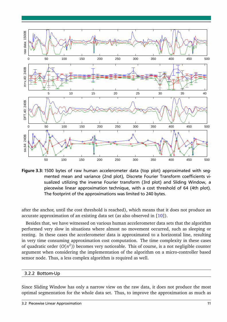
Figure 3.3: 1500 bytes of raw human accelerometer data (top plot) approximated with seg-mented mean and variance (2nd plot), Discrete Fourier Transform coefficients vi-sualized utilizing the inverse Fourier transform (3rd plot) and Sliding Window, apiecewise linear approximation technique, with a cost threshold of 64 (4th plot).The footprint of the approximations was limited to 240 bytes.

after the anchor, until the cost threshold is reached), which means that it does not produce anaccurate approximation of an existing data set (as also observed in [10]).

Besides that, we have witnessed on various human accelerometer data sets that the algorithmperformed very slow in situations where almost no movement occurred, such as sleeping orresting. In these cases the accelerometer data is approximated to a horizontal line, resultingin very time consuming approximation cost computation. The time complexity in these casesof quadratic order (O(n2)) becomes very noticeable. This of course, is a not negligible counterargument when considering the implementation of the algorithm on a micro-controller basedsensor node. Thus, a less complex algorithm is required as well.

3.2.2 Bottom-Up

Since Sliding Window has only a narrow view on the raw data, it does not produce the mostoptimal segmentation for the whole data set. Thus, to improve the approximation as much as


possible, another piecewise linear approximation algorithm was considered that is calculatedover the entire data set.

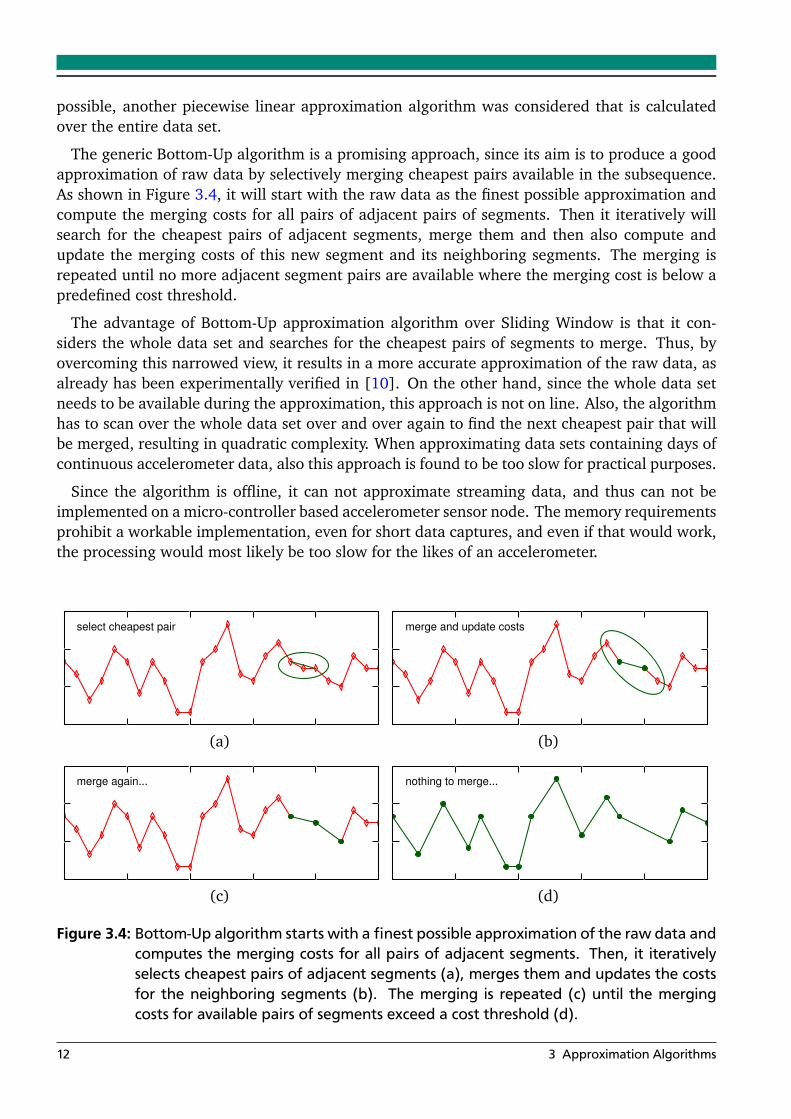
The generic Bottom-Up algorithm is a promising approach, since its aim is to produce a goodapproximation of raw data by selectively merging cheapest pairs available in the subsequence.As shown in Figure 3.4, it will start with the raw data as the finest possible approximation andcompute the merging costs for all pairs of adjacent pairs of segments. Then it iteratively willsearch for the cheapest pairs of adjacent segments, merge them and then also compute andupdate the merging costs of this new segment and its neighboring segments. The merging isrepeated until no more adjacent segment pairs are available where the merging cost is below apredefined cost threshold.

The advantage of Bottom-Up approximation algorithm over Sliding Window is that it con-siders the whole data set and searches for the cheapest pairs of segments to merge. Thus, byovercoming this narrowed view, it results in a more accurate approximation of the raw data, asalready has been experimentally verified in [10]. On the other hand, since the whole data setneeds to be available during the approximation, this approach is not on line. Also, the algorithmhas to scan over the whole data set over and over again to find the next cheapest pair that willbe merged, resulting in quadratic complexity. When approximating data sets containing days ofcontinuous accelerometer data, also this approach is found to be too slow for practical purposes.

Since the algorithm is offline, it can not approximate streaming data, and thus can not beimplemented on a micro-controller based accelerometer sensor node. The memory requirementsprohibit a workable implementation, even for short data captures, and even if that would work,the processing would most likely be too slow for the likes of an accelerometer.

select cheapest pair

(a)

merge and update costs

(b)

merge again...

(c)

nothing to merge...

(d)

Figure 3.4: Bottom-Up algorithm starts with a finest possible approximation of the raw data andcomputes the merging costs for all pairs of adjacent segments. Then, it iterativelyselects cheapest pairs of adjacent segments (a), merges them and updates the costsfor the neighboring segments (b). The merging is repeated (c) until the mergingcosts for available pairs of segments exceed a cost threshold (d).


3.2.3 SWAB: Sliding Window and Bottom-Up

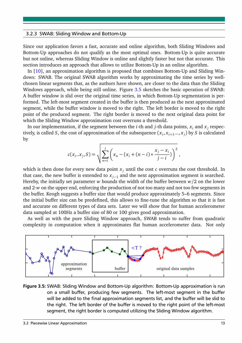
Since our application favors a fast, accurate and online algorithm, both Sliding Windows andBottom-Up approaches do not qualify as the most optimal ones. Bottom-Up is quite accuratebut not online, whereas Sliding Window is online and slightly faster but not that accurate. Thissection introduces an approach that allows to utilize Bottom-Up in an online algorithm.

In [10], an approximation algorithm is proposed that combines Bottom-Up and Sliding Win-dows: SWAB. The original SWAB algorithm works by approximating the time series by well-chosen linear segments that, as the authors have shown, are closer to the data than the SlidingWindows approach, while being still online. Figure 3.5 sketches the basic operation of SWAB:A buffer window is slid over the original time series, in which Bottom-Up segmentation is per-formed. The left-most segment created in the buffer is then produced as the next approximatedsegment, while the buffer window is moved to the right. The left border is moved to the rightpoint of the produced segment. The right border is moved to the next original data point forwhich the Sliding Window approximation cost overruns a threshold.

In our implementation, if the segment between the i-th and j-th data points, x i and x j respec-tively, is called S, the cost of approximation of the subsequence (x i, x i+1..., x j) by S is calculatedby

c(x i..x j, S) =

√

√

√

√

j∑

n=i

�

xn− (x i + (n− i) ∗x j − x i

j− i)�2

,

which is then done for every new data point x j until the cost c overruns the cost threshold. Inthat case, the new buffer is extended to x j−1 and the next approximation segment is searched.Hereby, the initially set parameter w bounds the width of the buffer between w/2 on the lowerand 2·w on the upper end, enforcing the production of not too many and not too few segments inthe buffer. Keogh suggests a buffer size that would produce approximately 5–6 segments. Sincethe initial buffer size can be predefined, this allows to fine-tune the algorithm so that it is fastand accurate on different types of data sets. Later we will show that for human accelerometerdata sampled at 100Hz a buffer size of 80 or 100 gives good approximation.

As well as with the pure Sliding Window approach, SWAB tends to suffer from quadraticcomplexity in computation when it approximates flat human accelerometer data. Not only

approximationsegments buffer original data samples

<T ?

Figure 3.5: SWAB: Sliding Window and Bottom-Up algorithm: Bottom-Up approximation is runon a small buffer, producing few segments. The left-most segment in the bufferwill be added to the final approximation segments list, and the buffer will be slid tothe right. The left border of the buffer is moved to the right point of the left-mostsegment, the right border is computed utilizing the Sliding Window algorithm.


Cost Threshold = 10

Buffer Size

Tim

e (%

of S

WA

B)

20 40 60 80 100 120 140 1600

0.1

0.2

0.3

0.4

0.5

0.6

0.7

0.8

0.9

1

Sliding Window

Bottom−Up

(a)

Cost Threshold

Tim

e (%

of S

WA

B)

Buffer Size = 100

2 4 6 8 10 12 14 160

0.1

0.2

0.3

0.4

0.5

0.6

0.7

0.8

0.9

1

Bottom−Up

Sliding Window

(b)

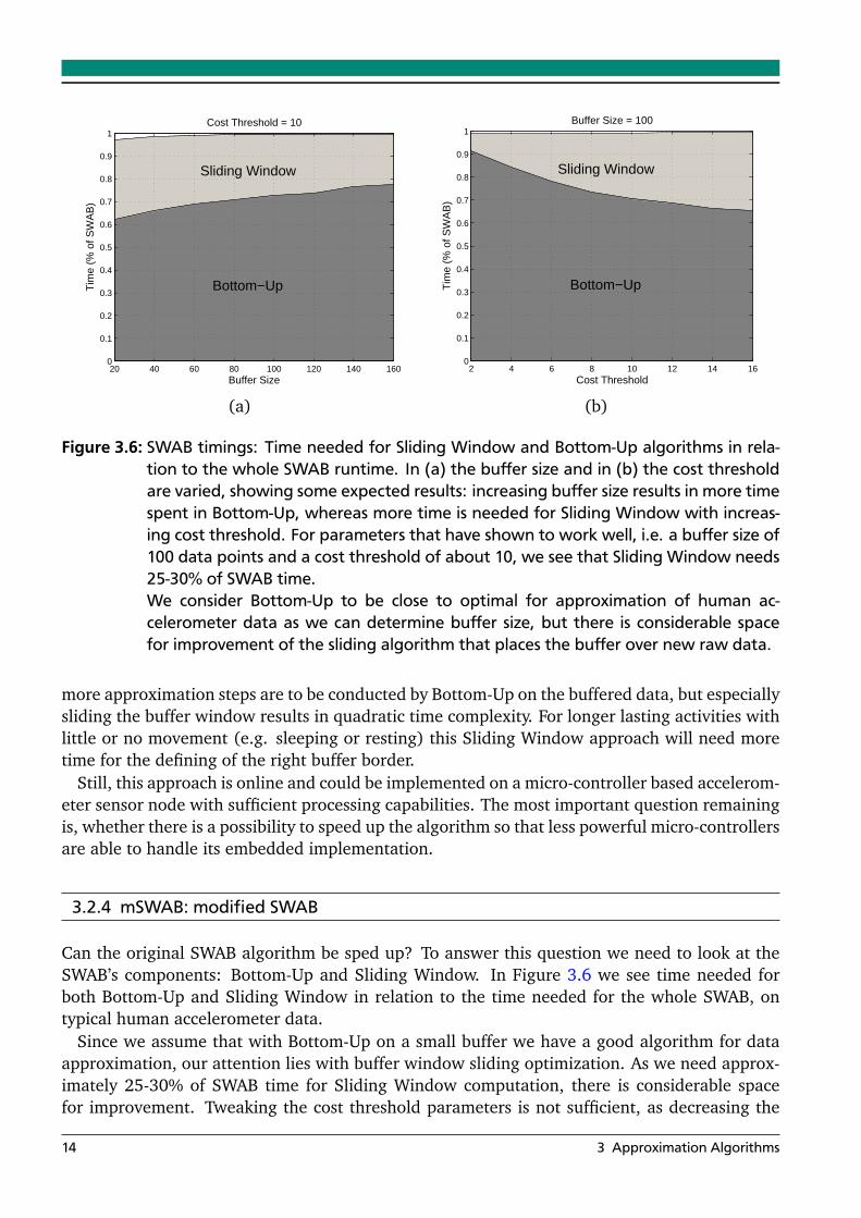
Figure 3.6: SWAB timings: Time needed for Sliding Window and Bottom-Up algorithms in rela-tion to the whole SWAB runtime. In (a) the buffer size and in (b) the cost thresholdare varied, showing some expected results: increasing buffer size results in more timespent in Bottom-Up, whereas more time is needed for Sliding Window with increas-ing cost threshold. For parameters that have shown to work well, i.e. a buffer size of100 data points and a cost threshold of about 10, we see that Sliding Window needs25-30% of SWAB time.We consider Bottom-Up to be close to optimal for approximation of human ac-celerometer data as we can determine buffer size, but there is considerable spacefor improvement of the sliding algorithm that places the buffer over new raw data.

more approximation steps are to be conducted by Bottom-Up on the buffered data, but especiallysliding the buffer window results in quadratic time complexity. For longer lasting activities withlittle or no movement (e.g. sleeping or resting) this Sliding Window approach will need moretime for the defining of the right buffer border.

Still, this approach is online and could be implemented on a micro-controller based accelerom-eter sensor node with sufficient processing capabilities. The most important question remainingis, whether there is a possibility to speed up the algorithm so that less powerful micro-controllersare able to handle its embedded implementation.

3.2.4 mSWAB: modified SWAB

Can the original SWAB algorithm be sped up? To answer this question we need to look at theSWAB’s components: Bottom-Up and Sliding Window. In Figure 3.6 we see time needed forboth Bottom-Up and Sliding Window in relation to the time needed for the whole SWAB, ontypical human accelerometer data.

Since we assume that with Bottom-Up on a small buffer we have a good algorithm for dataapproximation, our attention lies with buffer window sliding optimization. As we need approx-imately 25-30% of SWAB time for Sliding Window computation, there is considerable spacefor improvement. Tweaking the cost threshold parameters is not sufficient, as decreasing the


approximationsegments original data samplesbuffer

slope?

Figure 3.7: mSWAB, a modification of SWAB algorithm: Bottom-Up approximation is run ona small buffer, producing few segments. The left-most segment in the buffer willbe added to the approximation segments, and the buffer will be slid to the right,whereby the right border is computed using slope sign changes in raw data.

threshold will result in a higher overall runtime of SWAB as well as too fine approximation ofthe raw data and thus with a higher footprint of the approximation. The authors of [10] men-tion that optimizations are possible for particular data, by e.g. incrementing the sliding windowwith multiple samples instead of one (which showed beneficial in case of ECG data).

We, on the other hand, propose a modification that replaces the costly Sliding Window partof SWAB to compute the right border of the buffer window by using slope sign changes inraw data. Our adaptation exploits the property of accelerometer data, which tends to heavilyfluctuate during the characteristic peaks in the time series, and instead moves the window on tothe next data point where the slope’s sign changes between positive and negative, or switches tozero (Figure 3.7). Instead of having to iteratively calculate the approximation cost c, one simplyhas to calculate the slope between adjacent data points x j and x j+1 and stop when the sign ofthis slope changes.

This speeds up the process as it requires a single test per sample (O(n) with n the samples thebuffer is shifted over), instead of recalculating costs over the segment (O(n2) regardless whethersum of squares or the L∞ norm is used for the cost calculation). Although the Bottom-Up part ofSWAB remains still costly, substituting the Sliding Window approach leads to a significant effectwhen the accelerometer data is sampled at a high frequency or in constant subsequences (i.e.,when no movement occurs).

A second change to the original algorithm uses a suggestion made by [9] to merge the last twoproduced segments if their slope is the same. Listing 3.1 shows the source code, highlightingthe differences to the original SWAB algorithm.

Listing 3.1: Here, the original SWAB algorithm abstracting t imeseries with cost threshold T , hasthe Sliding Window heuristic modified to increase the algorithm’s speed. To createless data, segments with similar slopes are merged.� �

[ segs ] = mSWABsegs( t imese r i e s , len , T)w in _ l e f t =1; win_r ight=b u f s i z e ;while (1) % whi l e new data :

swabbuf=t i m e s e r i e s [ w i n_ l e f t : win_r ight ] ;% Bottom−Up segmenta t ion o f b u f f e r :BUsegs ( swabbuf , bu f s i ze , BUsegs , T ) ;% add l e f t −most segment from BU:segs = [ segs ; BUsegs ( 2 ) ] ; n = s ize ( segs ) ;


% merge l a s t segments i f s l o p e i s equa l :i f s lope ( segs (n )) == slope ( segs (n−1)) ,

merge_last2 ( segs ) ; n = n−1; end ;% s h i f t l e f t o f b u f f e r window :win _ l e f t = BUsegs ( 2 ) . x ;% s h i f t r i g h t o f b u f f e r window :i f ( win_r ight<len ) ,

i=win_r ight +1;s = sgn ( s lope ( i , i −1));while sgn ( s lope ( i , i−1))==s ) ,

i=i +1;end ;win_r ight=i ;b u f s i z e=win_right−win _ l e f t ;

else% a l l done , f l u s h b u f f e r segments :segs = [ segs ; BUsegs ] ;break ;

end ;end ;� �

Given the modified version of SWAB, the remaining question are: how does mSWAB performcompared to the original SWAB? We expect mSWAB to be faster, is it really the case? Is theapproximation delivered by mSWAB worse, as good as or better as SWAB’s? These questionswill be answered in section 6.1 that covers the experiments and results of some approximationalgorithms presented here.

3.3 Piecewise Polynomial Approximation

A cooperation with the University of Passau allowed us to actively share our algorithms imple-mentations and get hands on their online time series approximation approach [4]. The basicidea of the approach is to approximate raw data by piecewise polynomials (Figure 3.8) insteadof linear segments, as discussed above. Thus, the aim is to represent the raw data set by aparameterized function f that is a linear combination of K+1 linear or non-linear – as they callit – basis functions fk:

f : R→ R, f (x) =K∑

k=0

wk fk(x), whereby: ωk ∈ R, k = 1, . . . , K

The authors approach the approximation problem by utilizing the least-squares polynomialapproximation. Making some assumptions and claims (for detail please refer to their paper) itis then possible to approximate these basis functions by basis polynomials pk with k = 0, . . . , K .Thus, the approximating polynomial, that is a weighted sum of these basis polynomials, can benoted as:

p(x) =K∑

k=0

αk

||pk||2pk(x)


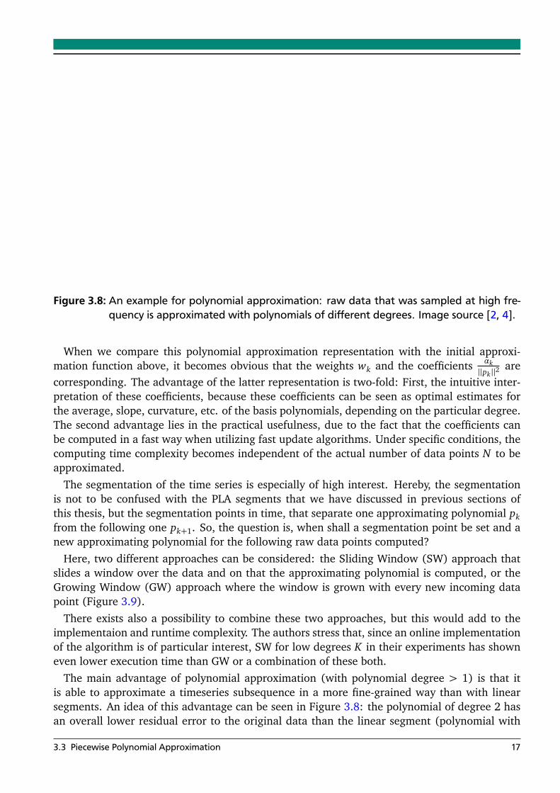
Figure 3.8: An example for polynomial approximation: raw data that was sampled at high fre-quency is approximated with polynomials of different degrees. Image source [2, 4].

When we compare this polynomial approximation representation with the initial approxi-mation function above, it becomes obvious that the weights wk and the coefficients αk

||pk||2are

corresponding. The advantage of the latter representation is two-fold: First, the intuitive inter-pretation of these coefficients, because these coefficients can be seen as optimal estimates forthe average, slope, curvature, etc. of the basis polynomials, depending on the particular degree.The second advantage lies in the practical usefulness, due to the fact that the coefficients canbe computed in a fast way when utilizing fast update algorithms. Under specific conditions, thecomputing time complexity becomes independent of the actual number of data points N to beapproximated.

The segmentation of the time series is especially of high interest. Hereby, the segmentationis not to be confused with the PLA segments that we have discussed in previous sections ofthis thesis, but the segmentation points in time, that separate one approximating polynomial pkfrom the following one pk+1. So, the question is, when shall a segmentation point be set and anew approximating polynomial for the following raw data points computed?

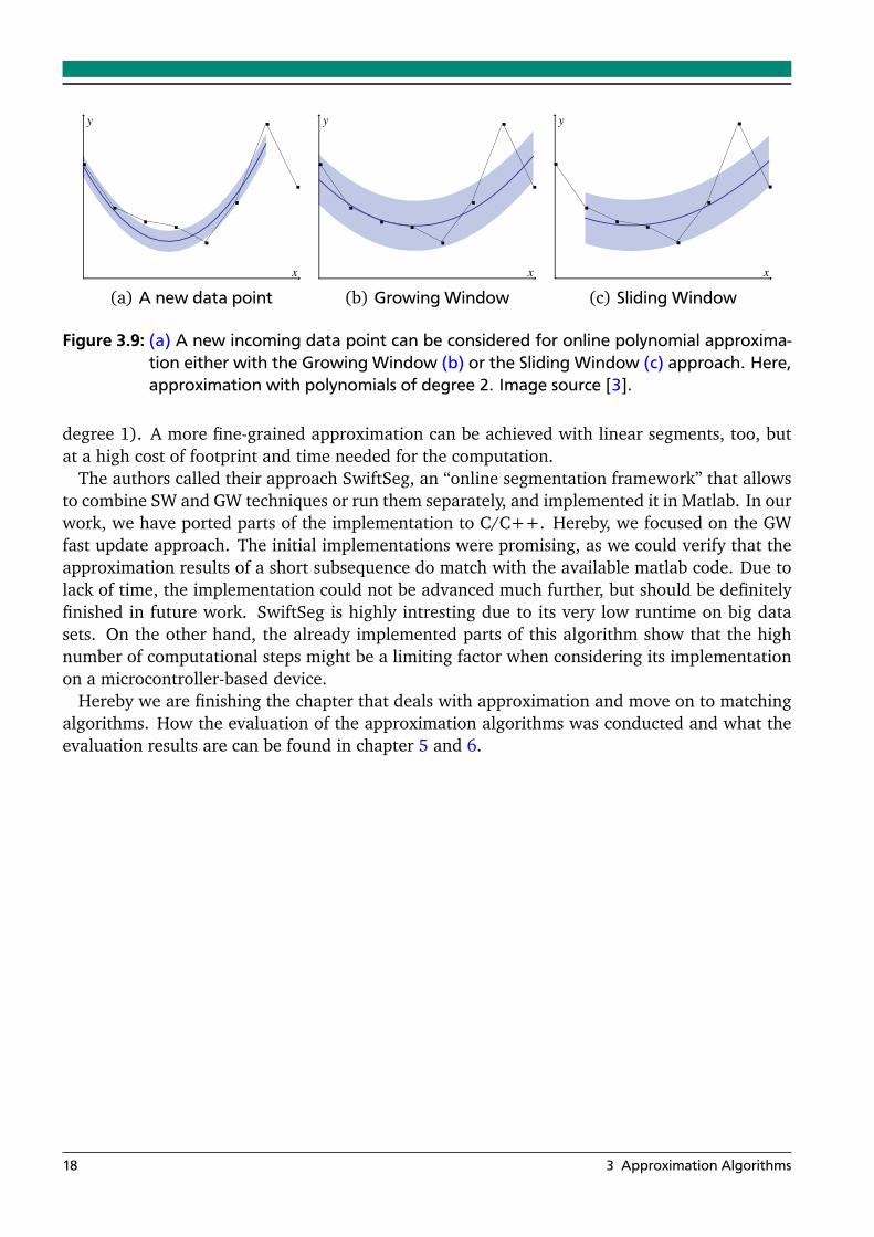
Here, two different approaches can be considered: the Sliding Window (SW) approach thatslides a window over the data and on that the approximating polynomial is computed, or theGrowing Window (GW) approach where the window is grown with every new incoming datapoint (Figure 3.9).

There exists also a possibility to combine these two approaches, but this would add to theimplementaion and runtime complexity. The authors stress that, since an online implementationof the algorithm is of particular interest, SW for low degrees K in their experiments has showneven lower execution time than GW or a combination of these both.

The main advantage of polynomial approximation (with polynomial degree > 1) is that itis able to approximate a timeseries subsequence in a more fine-grained way than with linearsegments. An idea of this advantage can be seen in Figure 3.8: the polynomial of degree 2 hasan overall lower residual error to the original data than the linear segment (polynomial with

3.3 Piecewise Polynomial Approximation 17

y

x

(a) A new data point

y

x

(b) Growing Window

y

x

(c) Sliding Window

Figure 3.9: (a) A new incoming data point can be considered for online polynomial approxima-tion either with the Growing Window (b) or the Sliding Window (c) approach. Here,approximation with polynomials of degree 2. Image source [3].

degree 1). A more fine-grained approximation can be achieved with linear segments, too, butat a high cost of footprint and time needed for the computation.

The authors called their approach SwiftSeg, an “online segmentation framework” that allowsto combine SW and GW techniques or run them separately, and implemented it in Matlab. In ourwork, we have ported parts of the implementation to C/C++. Hereby, we focused on the GWfast update approach. The initial implementations were promising, as we could verify that theapproximation results of a short subsequence do match with the available matlab code. Due tolack of time, the implementation could not be advanced much further, but should be definitelyfinished in future work. SwiftSeg is highly intresting due to its very low runtime on big datasets. On the other hand, the already implemented parts of this algorithm show that the highnumber of computational steps might be a limiting factor when considering its implementationon a microcontroller-based device.

Hereby we are finishing the chapter that deals with approximation and move on to matchingalgorithms. How the evaluation of the approximation algorithms was conducted and what theevaluation results are can be found in chapter 5 and 6.


4 Matching Algorithms

After looking at different approximation approaches, we now move on to matching algorithms.We need matching algorithms for two reasons: First, we want to evaluate the approximationalgorithms and their parameters discussed previously on how well they retain the essentials ofthe motion patterns in a classification setting. Second, we need accurate matching algorithmsto actually find closest matches to a query subsequence in a data set.

But, since we want to utilize matching to help users in annotating their own motion data,we also have to consider the speed of an matching algorithm. Finding closest matches musttherefore be as accurate and as fast as possible. A fast and reliable algorithm then will make itfeasible to support a person at the task of annotating his own data.

The following sections will present and discuss three matching and classification approaches.

4.1 Dynamic Time Warping

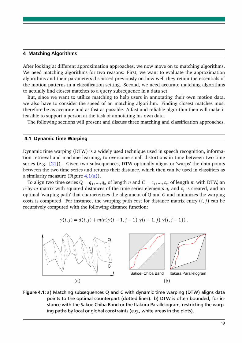
Dynamic time warping (DTW) is a widely used technique used in speech recognition, informa-tion retrieval and machine learning, to overcome small distortions in time between two timeseries (e.g. [21]) . Given two subsequences, DTW optimally aligns or ‘warps’ the data pointsbetween the two time series and returns their distance, which then can be used in classifiers asa similarity measure (Figure 4.1(a)).

To align two time series Q = q1, ..., qn of length n and C = c1, ..., cm of length m with DTW, ann-by-m matrix with squared distances of the time series elements qi and c j is created, and anoptimal ‘warping path’ that characterizes the alignment of Q and C and minimizes the warpingcosts is computed. For instance, the warping path cost for distance matrix entry (i, j) can berecursively computed with the following distance function:

γ(i, j) = d(i, j) +min{γ(i− 1, j− 1),γ(i− 1, j),γ(i, j− 1)} .

C

t

Q

(a)

Itakura ParallelogramSakoe−Chiba Band

(b)

Figure 4.1: a) Matching subsequences Q and C with dynamic time warping (DTW) aligns datapoints to the optimal counterpart (dotted lines). b) DTW is often bounded, for in-stance with the Sakoe-Chiba Band or the Itakura Parallelogram, restricting the warp-ing paths by local or global constraints (e.g., white areas in the plots).

19

The general approach, which computes all the squared distances in the matrix and choosesthe minimal continuous path, is of high time complexity (O(n ·m)). In practice, different localor global constraints can be used to decrease the number of paths that will be computed duringalignment process, thus significantly speeding up the calculation. In our implementations weconsidered two common bounding techniques: the Sakoe-Chiba Band [24] and the ItakuraParallelogram [8], where only paths are considered that lie within certain bounds (see Figure4.1(b)). Other lower bounding techniques as well as new approaches for DTW have been alsorecently discussed and presented in [23] and [14].

Since DTW has shown good results throughout its usage in scientific work, we use this match-ing approach (especially the Sakoe-Chiba band bounded version) as a reference for the matchingalgorithms we will be discussing in the following subsections. Because of the time characteristicof DTW and the requirement for a fast matching algorithm, to interactively support participatingsubject while their annotation task, we are interested in speeding up the matching process.

In the following, shape matching approaches will be presented that aim at reducing the com-putational complexity and speed up the matching. This comes at the cost of accuracy due to theability to warp time distortions (e.g. stretches in time) between two motion patterns. Althoughthis does not happen extensively in human accelerometer data, small shifts in time do occur.

4.2 K Longest Segments

Most subsequences of interest tend to have a high number of segments. Thus, computing thedistance or similarity measure with exhaustive approaches such as Euclidean matching or un-bounded / not sufficient bounded dynamic time warping will require significant amount of time.If we consider the initially mentioned aim to support a user where he interactively annotateshis own motion data, by searching and presenting closes matches for chosen patterns, we mustfocus on matching algorithms that are not only accurate but also fast.

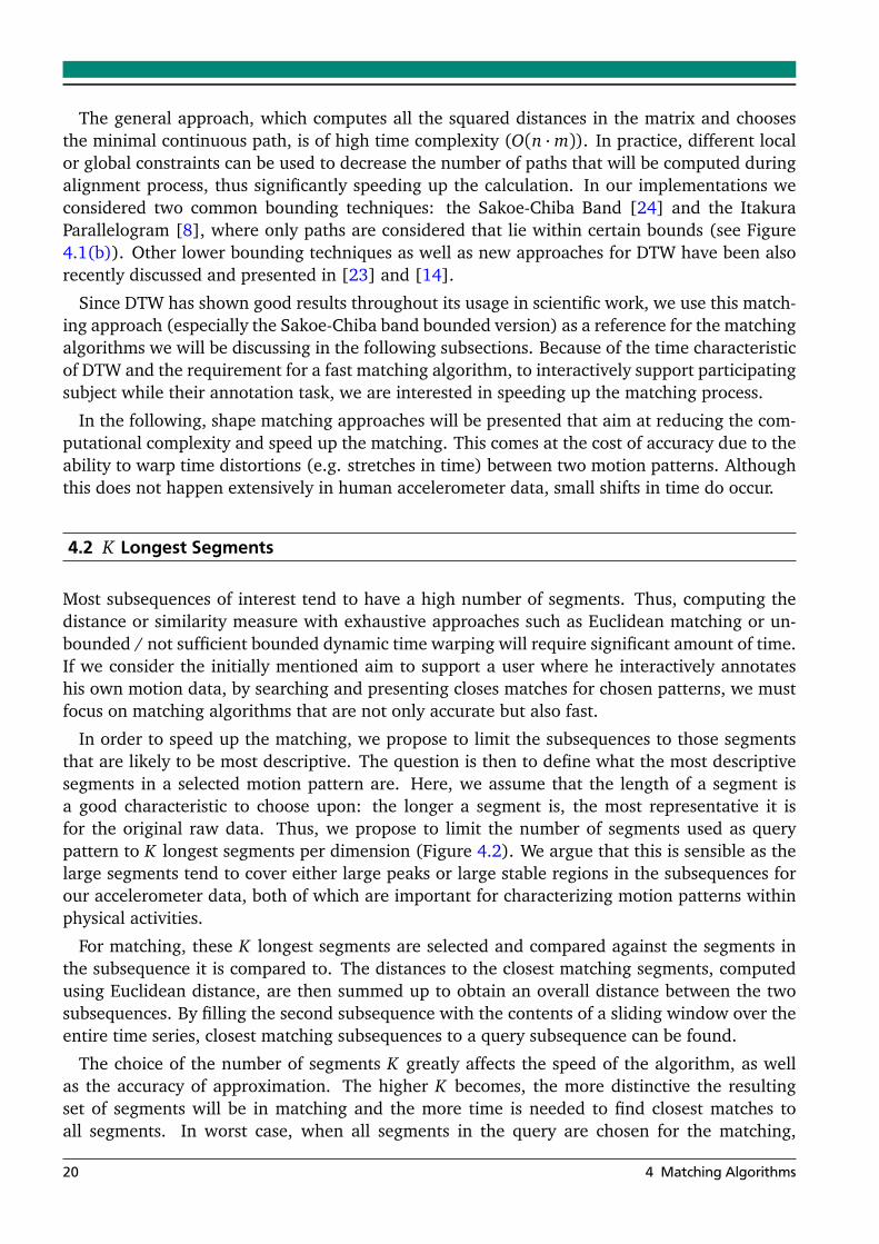
In order to speed up the matching, we propose to limit the subsequences to those segmentsthat are likely to be most descriptive. The question is then to define what the most descriptivesegments in a selected motion pattern are. Here, we assume that the length of a segment isa good characteristic to choose upon: the longer a segment is, the most representative it isfor the original raw data. Thus, we propose to limit the number of segments used as querypattern to K longest segments per dimension (Figure 4.2). We argue that this is sensible as thelarge segments tend to cover either large peaks or large stable regions in the subsequences forour accelerometer data, both of which are important for characterizing motion patterns withinphysical activities.

For matching, these K longest segments are selected and compared against the segments inthe subsequence it is compared to. The distances to the closest matching segments, computedusing Euclidean distance, are then summed up to obtain an overall distance between the twosubsequences. By filling the second subsequence with the contents of a sliding window over theentire time series, closest matching subsequences to a query subsequence can be found.

The choice of the number of segments K greatly affects the speed of the algorithm, as wellas the accuracy of approximation. The higher K becomes, the more distinctive the resultingset of segments will be in matching and the more time is needed to find closest matches toall segments. In worst case, when all segments in the query are chosen for the matching,

20 4 Matching Algorithms

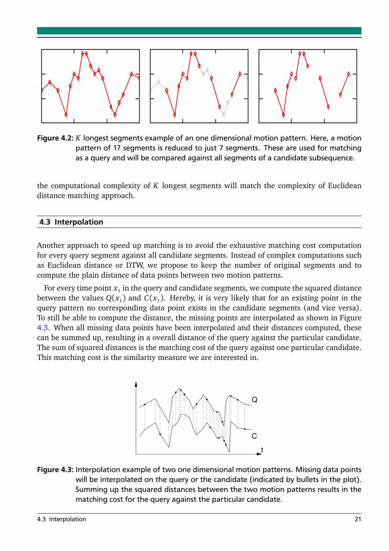
Figure 4.2: K longest segments example of an one dimensional motion pattern. Here, a motionpattern of 17 segments is reduced to just 7 segments. These are used for matchingas a query and will be compared against all segments of a candidate subsequence.

the computational complexity of K longest segments will match the complexity of Euclideandistance matching approach.

4.3 Interpolation

Another approach to speed up matching is to avoid the exhaustive matching cost computationfor every query segment against all candidate segments. Instead of complex computations suchas Euclidean distance or DTW, we propose to keep the number of original segments and tocompute the plain distance of data points between two motion patterns.

For every time point x t in the query and candidate segments, we compute the squared distancebetween the values Q(x t) and C(x t). Hereby, it is very likely that for an existing point in thequery pattern no corresponding data point exists in the candidate segments (and vice versa).To still be able to compute the distance, the missing points are interpolated as shown in Figure4.3. When all missing data points have been interpolated and their distances computed, thesecan be summed up, resulting in a overall distance of the query against the particular candidate.The sum of squared distances is the matching cost of the query against one particular candidate.This matching cost is the similarity measure we are interested in.

t

Q

C

Figure 4.3: Interpolation example of two one dimensional motion patterns. Missing data pointswill be interpolated on the query or the candidate (indicated by bullets in the plot).Summing up the squared distances between the two motion patterns results in thematching cost for the query against the particular candidate.

4.3 Interpolation 21

t

(a) Similar but stretched pattern

t

(b) Flat pattern with few segments

Figure 4.4: Interpolation matching with a similar but stretched pattern (a) and a non-similar pat-tern with few segments (b). The matching distance of a candidate with few segmentsoften was smaller than of a similar stretched pattern. To solve the issue, the numberof segments in the candidate pattern has to be considered.

By sliding the query window over the whole approximated data set, this algorithm will pro-duce matching costs for all possible candidates. By observing the matching cost, and by e.g.choosing the lowest one, we are able to classify patterns via the closest match.

This approach reduces the computational complexity, since it has n + m interpolations ofdata points for a query and a candidate in worst case. After the interpolation, the sum ofsquared distances needs to be computed. Resulting in a linear time complexity order against thequadratic complexity of Euclidean distance.

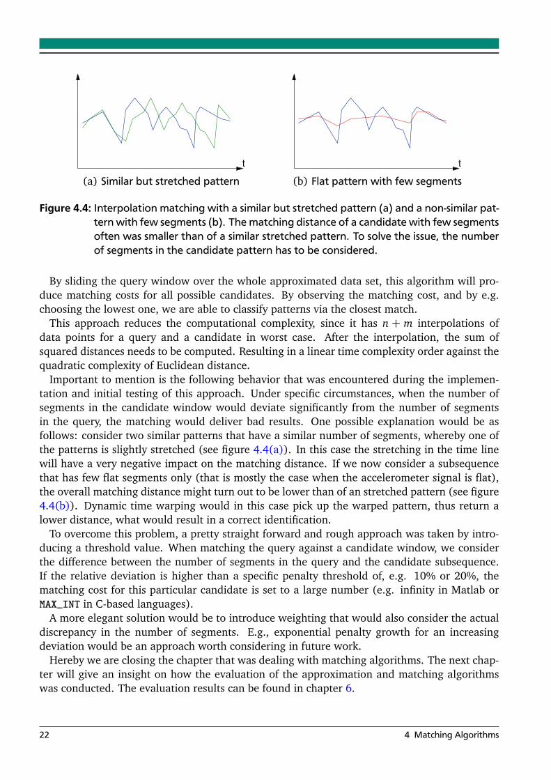
Important to mention is the following behavior that was encountered during the implemen-tation and initial testing of this approach. Under specific circumstances, when the number ofsegments in the candidate window would deviate significantly from the number of segmentsin the query, the matching would deliver bad results. One possible explanation would be asfollows: consider two similar patterns that have a similar number of segments, whereby one ofthe patterns is slightly stretched (see figure 4.4(a)). In this case the stretching in the time linewill have a very negative impact on the matching distance. If we now consider a subsequencethat has few flat segments only (that is mostly the case when the accelerometer signal is flat),the overall matching distance might turn out to be lower than of an stretched pattern (see figure4.4(b)). Dynamic time warping would in this case pick up the warped pattern, thus return alower distance, what would result in a correct identification.

To overcome this problem, a pretty straight forward and rough approach was taken by intro-ducing a threshold value. When matching the query against a candidate window, we considerthe difference between the number of segments in the query and the candidate subsequence.If the relative deviation is higher than a specific penalty threshold of, e.g. 10% or 20%, thematching cost for this particular candidate is set to a large number (e.g. infinity in Matlab orMAX_INT in C-based languages).

A more elegant solution would be to introduce weighting that would also consider the actualdiscrepancy in the number of segments. E.g., exponential penalty growth for an increasingdeviation would be an approach worth considering in future work.

Hereby we are closing the chapter that was dealing with matching algorithms. The next chap-ter will give an insight on how the evaluation of the approximation and matching algorithmswas conducted. The evaluation results can be found in chapter 6.

22 4 Matching Algorithms

5 Evaluation Methods

This chapter gives detailed insight on the evaluation method of the approximation and matchingalgorithms used in the next chapter. For the approximation, most important is to find a goodtrade-off in speed and accuracy. For the matching, special point of interest is the N -fold cross-validation conducted for the evaluation of the accuracy, precision and recall of the previouslydiscussed matching algorithms. The matching and classification evaluation itself is done with ageneric script that will be discussed in the following section.

5.1 Approximation

In this section we look at what is important when evaluating the performance of an approxi-mation algorithm and what needs to be compared to decide which algorithm performs betteror worse. As previously mentioned, we will leave out the traditional approximation approaches(mean and variance or DFT) as well as the polynomial approximation approach, and will con-centrate on PLA algorithms mostly.

With PLA algorithms we know that the visualization of the PLA approximation results is notconsidered a problem: the segments can be plotted like the original raw data in a time seriesplot in real-time. So the question that remains is: what do we need to look at to evaluate theperformance of the approximation algorithms mentioned above?

Following points are of particular interest:

• Accuracy of the approximation:How good are the produced segments approximating the raw data?

The accuracy of the approximation actually is a measure of how good the produced seg-ments approximate the raw data. One can and should expect that with an increasing ap-proximation or merging cost threshold the approximation accuracy will get worse, mean-ing a higher distance between the raw data points and their counter part, the interpolatedpoints on the segments.

Also, with a higher threshold, we can expect less segments to be produced, thus reducingthe footprint of the approximation. Obviously, we need an approximation, that on theone hand is accurate enough to capture the essence of the human motion, but reduces thefootprint on the other hand. Therefore, we already now have a trade-off between accuracyand footprint.

• Time requirements:How much time does the algorithm need to approximate a data set?

The time required for an approximation is very important when dealing with big datasets that contain continuous accelerometer data of multiple days. Faster approximationsare very preferred, especially because we want to use the approximation algorithms in ascenario with interactive setting. Also, a fast and efficient algorithm has a much betterchance to be implemented on a micro-controller based sensor device.

23

• Footprint of the approximation:How many segments have been produced by the algorithms?

The already mentioned footprint of an approximation is twofold interesting: On the onehand, a small amount of produced segments would allow to use the algorithms embeddedon a sensor device with limited memory. Also, this would result in less data to write ona memory card, reducing the battery power drain and resulting in a longer runtime. Theother aspect is important for the matching and classification, because with more segmentsproduced, more time is required for shape matching.

Considering these three points above, we therefore see us confronted with a trade-off be-tween the time required for computation of the accuracy and the footprint of an approximationalgorithm when conducted on available data sets.

The main approach to evaluate the approximation algorithms was to implement and run theseon already available data sets. For comparison purposes, all algorithms have been implementedin C/C++. A common Pentium 5 computer with 3.2GHz has been used for the approximationcalculations, whereby no other processor-consuming jobs were run. Two data sets have beenused for the evaluation: ADay that has almost 35 hours of continuous inertial data with vari-ous daily activities and different levels of activity, and Gardening that is a special short-lastinggardening activities session with constantly high levels of activity.

The results and the conclusions on the approximation algorithm evaluation will be presentedin the “experiments and results” chapter (6).

5.2 Matching and Classification

This section deals with the evaluation of the performance of the three matching algorithmspresented previously. To automate the N -fold cross-validation evaluation, a generic script hasbeen implemented, that is explained in detail to assure the experiments’ reproduceability. Beforegoing into the script details, let us first define the terminology and the variables that will be usedin the following subsections:

variable description

actXpY activity-person data sets stored as variables in the matlab.mat fileD total number of activity-person data sets available in the matlab.mat file rep-

resenting the entire data set.N total number of folds. Per fold, the n-th part of an activity-person data set will

be chosen as training and the rest as test data (n ∈ 1 . . . N). All evaluationshave been conducted with N = 10.

m number of non-overlapping training windows of width M with maximum vari-ance that are considered as training examples.

cw classification window with a fixed width of 500. This window is used forvoting for a particular class based upon the score (1–normalized matchingdistance). The highest score, thus the closest match, is chosen in nearest-neighbor classification.

After introducing and explaining these variables, we can go over to the methodology, on howwe actually do the data splitting, and then will discuss the evaluation script in detail.

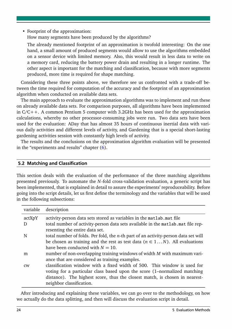
24 5 Evaluation Methods

5.2.1 Methodology

We discuss the N -fold cross-validation in this chapter, because it is a very important and widelyused tool when it comes to evaluation of classification approaches. Most scientific publicationsonly mention that an N -fold or leave one out cross-validation has been conducted and the resultsare presented, but often detailed information is left out, on how the data is split up.

To make our results comprehensible and reproduceable, the following approach is used forevaluation:

• For every fold the n-th part of every data set will be chosen as training part, and the rest astesting parts. These parts are approximated using a PLA algorithm presented previously,e.g. mSWAB.

• After approximation, the m highest variance patterns with fixed width M are taken fromevery training part and act as queries for matching.

• These queries are then matched against all available testing parts, resulting in matchingcosts. These matching costs are converted to scores by normalizing them over the wholetesting data and subtracting them from 1.

• Using these scores, nearest neighbor classification is conducted and smoothed over timeusing a window of size cw.

• By comparing the predictions with the actual labels, confusion matrices are created.

• On basis of these confusion matrices we can compute the accuracy, precision and recall forevery fold.

• Once all folds have been computed, we are able to compute average values for accuracy,precision and recall that represent the performance of approximation and matching for agiven combination of parameters.

To automate the evaluation procedure for any available data set, the steps described abovehave been incorporated into a matlab script. This generic evaluation script will be discussed inthe following subsection.

5.2.2 Generic Evaluation Script

This section deals with the evaluation script and will step by step go through its design, explain-ing how it splits up the data set and return its evaluation measures. For a more detailed insight,especially its concrete implementation, please refer to the Matlab source code and the existingdocumentation in the comments.

The evaluation script assumes that we have a set of Matlab variables for activity-person datasets stored in a matlab.mat file and that these variables are labeled as actXpY. For activity 5and person 2 the corresponding variable holding the raw accelerometer data therefore will benamed act5p2. Let us assume there are D such data set variables available. Once the scriptis started, it will conduct an N fold cross-validation, computing accuracy, precision and recallfor every fold. When finished, averaged values for all N folds will be computed, too, giving anoverall performance of the matching.

5.2 Matching and Classification 25

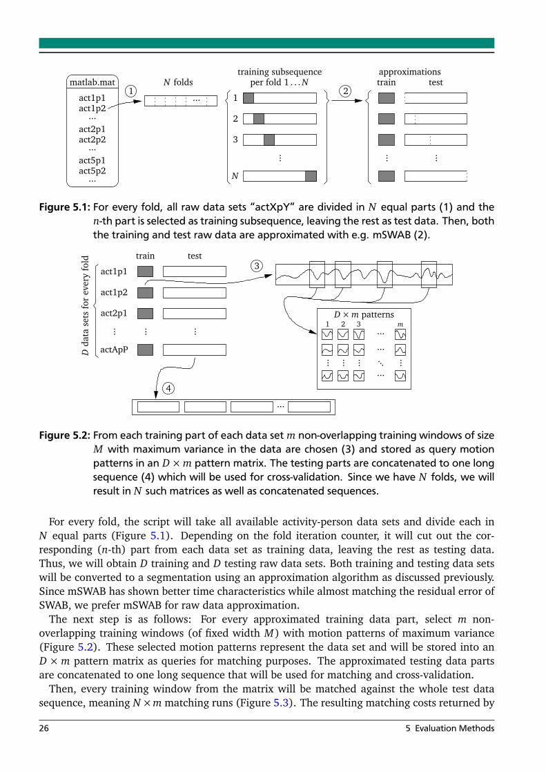
2...

1

2

N

3

1

...

train

... ...

testtraining subsequence

per fold 1 . . . Napproximations

N foldsmatlab.mat

act1p1act1p2

...

act5p1act5p2

act2p1act2p2

...

...

Figure 5.1: For every fold, all raw data sets “actXpY” are divided in N equal parts (1) and then-th part is selected as training subsequence, leaving the rest as test data. Then, boththe training and test raw data are approximated with e.g. mSWAB (2).

3

4

... ... ... ...

...

...

...

...

...

train

... ...

test

actApP

act1p1

act1p2

act2p1

...

D×m patterns1 2 3 m

Dda

tase

tsfo

rev

ery

fold

Figure 5.2: From each training part of each data set m non-overlapping training windows of sizeM with maximum variance in the data are chosen (3) and stored as query motionpatterns in an D×m pattern matrix. The testing parts are concatenated to one longsequence (4) which will be used for cross-validation. Since we have N folds, we willresult in N such matrices as well as concatenated sequences.

For every fold, the script will take all available activity-person data sets and divide each inN equal parts (Figure 5.1). Depending on the fold iteration counter, it will cut out the cor-responding (n-th) part from each data set as training data, leaving the rest as testing data.Thus, we will obtain D training and D testing raw data sets. Both training and testing data setswill be converted to a segmentation using an approximation algorithm as discussed previously.Since mSWAB has shown better time characteristics while almost matching the residual error ofSWAB, we prefer mSWAB for raw data approximation.

The next step is as follows: For every approximated training data part, select m non-overlapping training windows (of fixed width M) with motion patterns of maximum variance(Figure 5.2). These selected motion patterns represent the data set and will be stored into anD × m pattern matrix as queries for matching purposes. The approximated testing data partsare concatenated to one long sequence that will be used for matching and cross-validation.

Then, every training window from the matrix will be matched against the whole test datasequence, meaning N×m matching runs (Figure 5.3). The resulting matching costs returned by


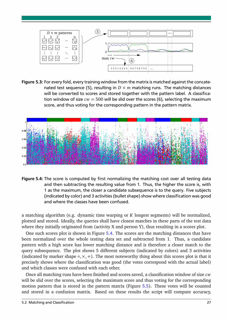
5

6

... ... ... ...

...

...

...

...

1 3 m...

33 3 31 2 2 4 6 6 7 8 7 55 5 ...

1

0

2

max cw

D×m patterns

Figure 5.3: For every fold, every training window from the matrix is matched against the concate-nated test sequence (5), resulting in D ×m matching runs. The matching distanceswill be converted to scores and stored together with the pattern label. A classifica-tion window of size cw = 500 will be slid over the scores (6), selecting the maximumscore, and thus voting for the corresponding pattern in the pattern matrix.

Figure 5.4: The score is computed by first normalizing the matching cost over all testing dataand then subtracting the resulting value from 1. Thus, the higher the score is, with1 as the maximum, the closer a candidate subsequence is to the query. Five subjects(indicated by color) and 3 activities (bullet shape) show where classification was goodand where the classes have been confused.

a matching algorithm (e.g. dynamic time warping or K longest segments) will be normalized,plotted and stored. Ideally, the queries shall have closest matches in these parts of the test datawhere they initially originated from (activity X and person Y), thus resulting in a scores plot.

One such scores plot is shown in Figure 5.4. The scores are the matching distances that havebeen normalized over the whole testing data set and subtracted from 1. Thus, a candidatepattern with a high score has lower matching distance and is therefore a closer match to thequery subsequence. The plot shows 5 different subjects (indicated by colors) and 3 activities(indicated by marker shape ◦,×,+). The most noteworthy thing about this scores plot is that itprecisely shows where the classification was good (the votes correspond with the actual label)and which classes were confused with each other.

Once all matching runs have been finished and scores saved, a classification window of size cwwill be slid over the scores, selecting the maximum score and thus voting for the correspondingmotion pattern that is stored in the pattern matrix (Figure 5.5). These votes will be countedand stored in a confusion matrix. Based on these results the script will compute accuracy,


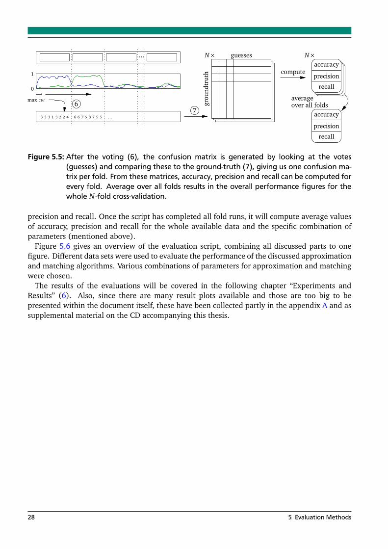
76

precision

accuracy

recall

...

max cw

33 3 31 2 2 4 6 6 7 8 7 55 5

1

0

...

N× guesses

grou

ndtr

uth compute

N×

precision

accuracy

recall

over all foldsaverage

Figure 5.5: After the voting (6), the confusion matrix is generated by looking at the votes(guesses) and comparing these to the ground-truth (7), giving us one confusion ma-trix per fold. From these matrices, accuracy, precision and recall can be computed forevery fold. Average over all folds results in the overall performance figures for thewhole N -fold cross-validation.

precision and recall. Once the script has completed all fold runs, it will compute average valuesof accuracy, precision and recall for the whole available data and the specific combination ofparameters (mentioned above).

Figure 5.6 gives an overview of the evaluation script, combining all discussed parts to onefigure. Different data sets were used to evaluate the performance of the discussed approximationand matching algorithms. Various combinations of parameters for approximation and matchingwere chosen.

The results of the evaluations will be covered in the following chapter “Experiments andResults” (6). Also, since there are many result plots available and those are too big to bepresented within the document itself, these have been collected partly in the appendix A and assupplemental material on the CD accompanying this thesis.


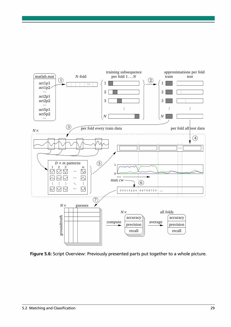
1 21

N

2

3

1

N

2

3

3

7

5

4

6

matlab.mat

act1p1act1p2

...

...

train

... ...

test

act5p1act5p2

act2p1act2p2

...

...

per fold 1 . . . Ntraining subsequence

N -fold

...

approximations per fold

N× per fold every train data

... ... ... ...

...

...

...

...

D×m patterns1 2 3 m

N× guesses

grou

ndtr

uth

compute

N×

averageprecision

accuracyall folds

precision

accuracy

recall recall

...

33 3 31 2 2 4 6 6 7 8 7 55 5 ...

1

0

max cw

per fold all test data

Figure 5.6: Script Overview: Previously presented parts put together to a whole picture.


6 Experiments and Results

This chapter covers the experiments that have been conducted with the implemented approxi-mation and matching algorithms. First, we will look at the performance and results of piecewiselinear approximation algorithms, and in particular those of our proposed modification, mSWAB.Then, matching and classification algorithm performance of dynamic time warping, K longestsegments and interpolation will be presented.

6.1 Approximation

As already mentioned previously in section 5.1, to evaluate approximation algorithms two datasets have been used. The main motivation behind using these different data sets is, first of alltheir difference in size and duration and, second, their inherent characteristics:

ADay This data set is a collection of three different data sets of 24, 34.5 and up to 49 hours ofcontinuous human accelerometer data. The 34.5 hours data set is a total of 38.582.922bytes. All data sets contain regular daily activities, such as walking, sleeping, office work,cooking, eating and drinking. Levels of activity therefore vary a lot: high levels of activitywhen cooking or conducting household activities, and low level of activity during the night.

Gardening This data set of approximately 20 minutes of continuous human accelerometer datahas been acquired when a person was performing gardening activities. This is a specificsetting with special activities and a constantly high level of activity, without lasting pauses.Since the activities were carried out without pauses, there is almost no flat data, whichcompasses e.g. resting or sleeping phases.

To recall from previous chapter, we are interested in looking at the following three resultswhen evaluating approximation algorithms: the accuracy of the approximation, the time re-quirements and the footprint of the approximation.

In the following subsections we will be looking at two different tests: an initial one that wasaiming solely at the time the algorithms needed to approximate a large raw data set, and a moreextended second test that was considering all three points of our interest.

6.1.1 Initial Test - Runtime

Let us first start with the execution time results of the algorithms presented previously in thisthesis.

Table 6.1 shows the time (in seconds) it takes for the various algorithms to approximate 24hours of accelerometer data, averaged over all days in the data set. For the results in the firstthree columns, the parameters of the respective algorithms are set so that the amounts of datathat each algorithm produces are approximately equal.

The results show that our modified version of SWAB is indeed faster than regular SWAB, muchfaster than DFT or Sliding Windows, yet a lot slower than the segmented mean and variance.

31

Table 6.1: Approximation methods and the time it takes to approximate the original raw. The2nd–4th columns vary the parameters so that the algorithms produce respectivelyhalf, a tenth, a twentieth of data representing the original raw data. The last columnshows how many seconds the algorithms need to transform a day worth of data (onaverage, with best parameters).

time to reduce 24h by time to processAlgorithm 50% 10% 5% 24 hours of data

Discrete Fourier 219 383 428 318Sliding Window 2.7 6.7 14 188.8Mean and Variance 0.1 0.1 0.1 0.1SWAB 8 7.7 7.9 36.1mSWAB 6.8 2.4 2.1 19.2

Implementing mSWAB on a microcontroller is feasible, however, as it does not require floatingpoint arithmetic, nor large data buffers.

With these preliminary results in the time domain, we want to have a closer look at how the al-gorithms perform in terms of the two other points of interest: the accuracy of the approximationand its actual footprint.

6.1.2 Extended Test - Accuracy, Runtime, Footprint

Since this thesis is focusing on PLA algorithms, Sliding Window, SWAB and mSWAB will bediscussed more closely in the following comparisons, leaving the traditional features approaches(DFT and Mean and Variance) out of the scope.

The following approximation experiments have been conducted on the 34.5 hours data setfrom the ADay collection [13]. Hereby we are not only looking at the execution time, as inthe initial test before, but consider the accuracy of the resulting approximation as well as theresulting footprint. Obviously, the cost threshold parameter has been varied: approximationcost threshold for Sliding Window and the merging cost threshold for the Bottom-Up algorithmthat is utilized to approximate the buffered data in SWAB and mSWAB. Hereby, the initial buffersize was set to 100, which is essentially the amount of raw data streaming in per second. Priorverification has shown that this value works well and contains the recommended 5 to 6 segmentsmentioned by Keogh in [10].

The left plots in Figure 6.1(a) and Figure 6.1(b) show the residual error (i.e., the sum ofsquares of the vertical differences between original data and approximation segment, for allsegments) for the Sliding Window, the SWAB algorithm, and the proposed mSWAB algorithm,for a cost threshold set between 1 and 50. There is little difference between the performances ofSWAB and mSWAB, confirming that the Bottom-Up buffer within the algorithm works identicallyfor both implementations. The results also further confirm those from [10], showing that theapproximation segments from the Sliding Windows algorithm are further apart from the originaldata than those of SWAB and mSWAB.

The right plot in Figure 6.1(a) shows the execution speed in seconds, for the cost thresholdof the approximation algorithms between 1 and 50. Identically to the residual error plot, the

32 6 Experiments and Results

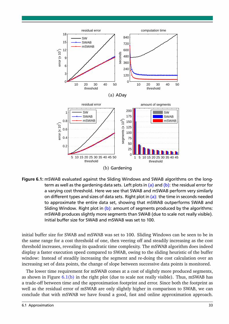
10 20 30 40 500

3

6

9

12

15

18residual error

threshold

erro

r (x

107 )

SWSWABmSWAB

10 20 30 40 500

120

240

360

480

600

720

840

computation time

threshold

seco

nds

(a) ADay

5 10 15 20 25 30 35 40 45 50

0.2

0.4

0.6

0.8

1

residual error

threshold

erro

r (x

107 )

SWSWABmSWAB

1 5 10 15 20 25 30 35 40 450

25

50

75

100

125

150

175

200

amount of segments

threshold

segm

ents

(x

103 )

SWSWABmSWAB

(b) Gardening

Figure 6.1: mSWAB evaluated against the Sliding Windows and SWAB algorithms on the long-term as well as the gardening data sets. Left plots in (a) and (b): the residual error fora varying cost threshold. Here we see that SWAB and mSWAB perform very similarlyon different types and sizes of data sets. Right plot in (a): the time in seconds neededto approximate the entire data set, showing that mSWAB outperforms SWAB andSliding Window. Right plot in (b): amount of segments produced by the algorithms:mSWAB produces slightly more segments than SWAB (due to scale not really visible).Initial buffer size for SWAB and mSWAB was set to 100.

initial buffer size for SWAB and mSWAB was set to 100. Sliding Windows can be seen to be inthe same range for a cost threshold of one, then veering off and steadily increasing as the costthreshold increases, revealing its quadratic time complexity. The mSWAB algorithm does indeeddisplay a faster execution speed compared to SWAB, owing to the sliding heuristic of the bufferwindow: Instead of steadily increasing the segment and re-doing the cost calculation over anincreasing set of data points, the change of slope between successive data points is monitored.

The lower time requirement for mSWAB comes at a cost of slightly more produced segments,as shown in Figure 6.1(b) in the right plot (due to scale not really visible). Thus, mSWAB hasa trade-off between time and the approximation footprint and error. Since both the footprint aswell as the residual error of mSWAB are only slightly higher in comparison to SWAB, we canconclude that with mSWAB we have found a good, fast and online approximation approach.

6.1 Approximation 33

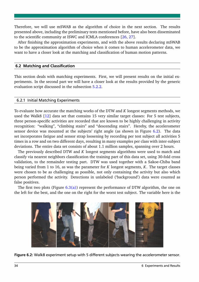
Therefore, we will use mSWAB as the algorithm of choice in the next section. The resultspresented above, including the preliminary tests mentioned before, have also been disseminatedto the scientific community at ISWC and ICMLA conferences [26, 27].

After finishing the approximation experiments, and with the above results declaring mSWABto be the approximation algorithm of choice when it comes to human accelerometer data, wewant to have a closer look at the matching and classification of human motion patterns.

6.2 Matching and Classification

This section deals with matching experiments. First, we will present results on the initial ex-periments. In the second part we will have a closer look at the results provided by the genericevaluation script discussed in the subsection 5.2.2.

6.2.1 Initial Matching Experiments

To evaluate how accurate the matching works of the DTW and K longest segments methods, weused the Walk8 [12] data set that contains 15 very similar target classes: For 5 test subjects,three person-specific activities are recorded that are known to be highly challenging in activityrecognition: “walking”, “climbing stairs” and “descending stairs”. Hereby, the accelerometersensor device was mounted at the subjects’ right angle (as shown in Figure 6.2). The dataset incorporates fatigue and sensor strap loosening by recording per test subject all activities 5times in a row and on two different days, resulting in many examples per class with inter-subjectdeviations. The entire data set consists of about 1.1 million samples, spanning over 2 hours.

The previously described DTW and K longest segments algorithms were used to match andclassify via nearest neighbors classification the training part of this data set, using 30-fold crossvalidation, to the remainder testing part. DTW was used together with a Sakoe-Chiba bandbeing varied from 1 to 16, as was the parameter for K longest segments, K . The target classeswere chosen to be as challenging as possible, not only containing the activity but also whichperson performed the activity. Detections in unlabeled (‘background’) data were counted asfalse positives.

The first two plots (Figure 6.3(a)) represent the performance of DTW algorithm, the one onthe left for the best, and the one on the right for the worst test subject. The variable here is the

Figure 6.2: Walk8 experiment setup with 5 different subjects wearing the accelerometer sensor.


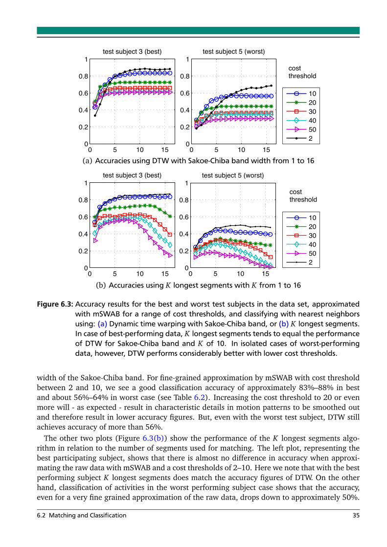
0 5 10 150

0.2

0.4

0.6

0.8

1test subject 3 (best)

0 5 10 150

0.2

0.4

0.6

0.8

1test subject 5 (worst)

10

20

30

40

50

2

costthreshold

(a) Accuracies using DTW with Sakoe-Chiba band width from 1 to 16

0 5 10 150

0.2

0.4

0.6

0.8

1test subject 3 (best)

0 5 10 150

0.2

0.4

0.6

0.8

1test subject 5 (worst)

10203040502

cost threshold

(b) Accuracies using K longest segments with K from 1 to 16

Figure 6.3: Accuracy results for the best and worst test subjects in the data set, approximatedwith mSWAB for a range of cost thresholds, and classifying with nearest neighborsusing: (a) Dynamic time warping with Sakoe-Chiba band, or (b) K longest segments.In case of best-performing data, K longest segments tends to equal the performanceof DTW for Sakoe-Chiba band and K of 10. In isolated cases of worst-performingdata, however, DTW performs considerably better with lower cost thresholds.

width of the Sakoe-Chiba band. For fine-grained approximation by mSWAB with cost thresholdbetween 2 and 10, we see a good classification accuracy of approximately 83%–88% in bestand about 56%–64% in worst case (see Table 6.2). Increasing the cost threshold to 20 or evenmore will - as expected - result in characteristic details in motion patterns to be smoothed outand therefore result in lower accuracy figures. But, even with the worst test subject, DTW stillachieves accuracy of more than 56%.

The other two plots (Figure 6.3(b)) show the performance of the K longest segments algo-rithm in relation to the number of segments used for matching. The left plot, representing thebest participating subject, shows that there is almost no difference in accuracy when approxi-mating the raw data with mSWAB and a cost thresholds of 2–10. Here we note that with the bestperforming subject K longest segments does match the accuracy figures of DTW. On the otherhand, classification of activities in the worst performing subject case shows that the accuracy,even for a very fine grained approximation of the raw data, drops down to approximately 50%.


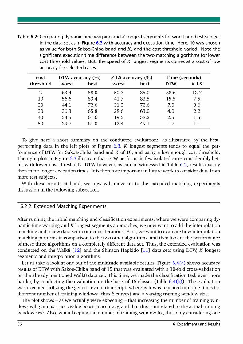
Table 6.2: Comparing dynamic time warping and K longest segments for worst and best subjectin the data set as in Figure 6.3 with accuracy and execution time. Here, 10 was chosenas value for both Sakoe-Chiba band and K , and the cost threshold varied. Note thesignificant execution time difference between the two matching algorithms for lowercost threshold values. But, the speed of K longest segments comes at a cost of lowaccuracy for selected cases.

cost DTW accuracy (%) K LS accuracy (%) Time (seconds)threshold worst best worst best DTW K LS

2 63.4 88.0 50.3 85.0 88.6 12.710 56.6 83.4 41.7 83.5 15.5 7.520 44.1 72.6 31.2 72.6 7.0 3.630 36.3 65.8 28.6 63.0 4.0 2.240 34.5 61.6 19.5 58.2 2.5 1.550 29.7 61.0 12.4 49.1 1.7 1.1

To give here a short summary on the conducted evaluation: as illustrated by the best-performing data in the left plots of Figure 6.3, K longest segments tends to equal the per-formance of DTW for Sakoe-Chiba band and K of 10, and using a low enough cost threshold.The right plots in Figure 6.3 illustrate that DTW performs in few isolated cases considerably bet-ter with lower cost thresholds. DTW however, as can be witnessed in Table 6.2, results exactlythen in far longer execution times. It is therefore important in future work to consider data frommore test subjects.

With these results at hand, we now will move on to the extended matching experimentsdiscussion in the following subsection.

6.2.2 Extended Matching Experiments

After running the initial matching and classification experiments, where we were comparing dy-namic time warping and K longest segments approaches, we now want to add the interpolationmatching and a new data set to our considerations. First, we want to evaluate how interpolationmatching performs in comparison to the two other algorithms, and then look at the performanceof these three algorithms on a completely different data set. Thus, the extended evaluation wasconducted on the Walk8 [12] and the Shinson Hapkido [11] data sets using DTW, K longestsegments and interpolation algorithms.

Let us take a look at one out of the multitude available results. Figure 6.4(a) shows accuracyresults of DTW with Sakoe-Chiba band of 15 that was evaluated with a 10-fold cross-validationon the already mentioned Walk8 data set. This time, we made the classification task even moreharder, by conducting the evaluation on the basis of 15 classes (Table 6.4(b)). The evaluationwas executed utilizing the generic evaluation script, whereby it was repeated multiple times fordifferent number of training windows (thus 6 curves) and a varying training window size.

The plot shows – as we actually were expecting – that increasing the number of training win-dows will gain us a noticeable boost in accuracy, and that this is unrelated to the actual trainingwindow size. Also, when keeping the number of training window fix, thus only considering one


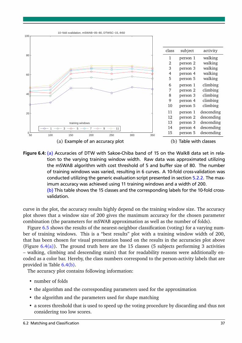
50 100 150 200 250 300 3500

20

40

60

80

10010−fold xvalidation, mSWAB−05−80, DTWSC−15, th50

1 3 5 7 9 11

training windows

(a) Example of an accuracy plot

class subject activity

1 person 1 walking2 person 2 walking3 person 3 walking4 person 4 walking5 person 5 walking

6 person 1 climbing7 person 2 climbing8 person 3 climbing9 person 4 climbing10 person 5 climbing

11 person 1 descending12 person 2 descending13 person 3 descending14 person 4 descending15 person 5 descending

(b) Table with classes

Figure 6.4: (a) Accuracies of DTW with Sakoe-Chiba band of 15 on the Walk8 data set in rela-tion to the varying training window width. Raw data was approximated utilizingthe mSWAB algorithm with cost threshold of 5 and buffer size of 80. The numberof training windows was varied, resulting in 6 curves. A 10-fold cross-validation wasconducted utilizing the generic evaluation script presented in section 5.2.2. The max-imum accuracy was achieved using 11 training windows and a width of 200.(b) This table shows the 15 classes and the corresponding labels for the 10-fold cross-validation.

curve in the plot, the accuracy results highly depend on the training window size. The accuracyplot shows that a window size of 200 gives the maximum accuracy for the chosen parametercombination (the parameters for mSWAB approximation as well as the number of folds).

Figure 6.5 shows the results of the nearest-neighbor classification (voting) for a varying num-ber of training windows. This is a “best results” plot with a training window width of 200,that has been chosen for visual presentation based on the results in the accuracies plot above(Figure 6.4(a)). The ground truth here are the 15 classes (5 subjects performing 3 activities– walking, climbing and descending stairs) that for readability reasons were additionally en-coded as a color bar. Hereby, the class numbers correspond to the person-activity labels that areprovided in Table 6.4(b).

The accuracy plot contains following information:

• number of folds

• the algorithm and the corresponding parameters used for the approximation

• the algorithm and the parameters used for shape matching

• a scores threshold that is used to speed up the voting procedure by discarding and thus notconsidering too low scores.


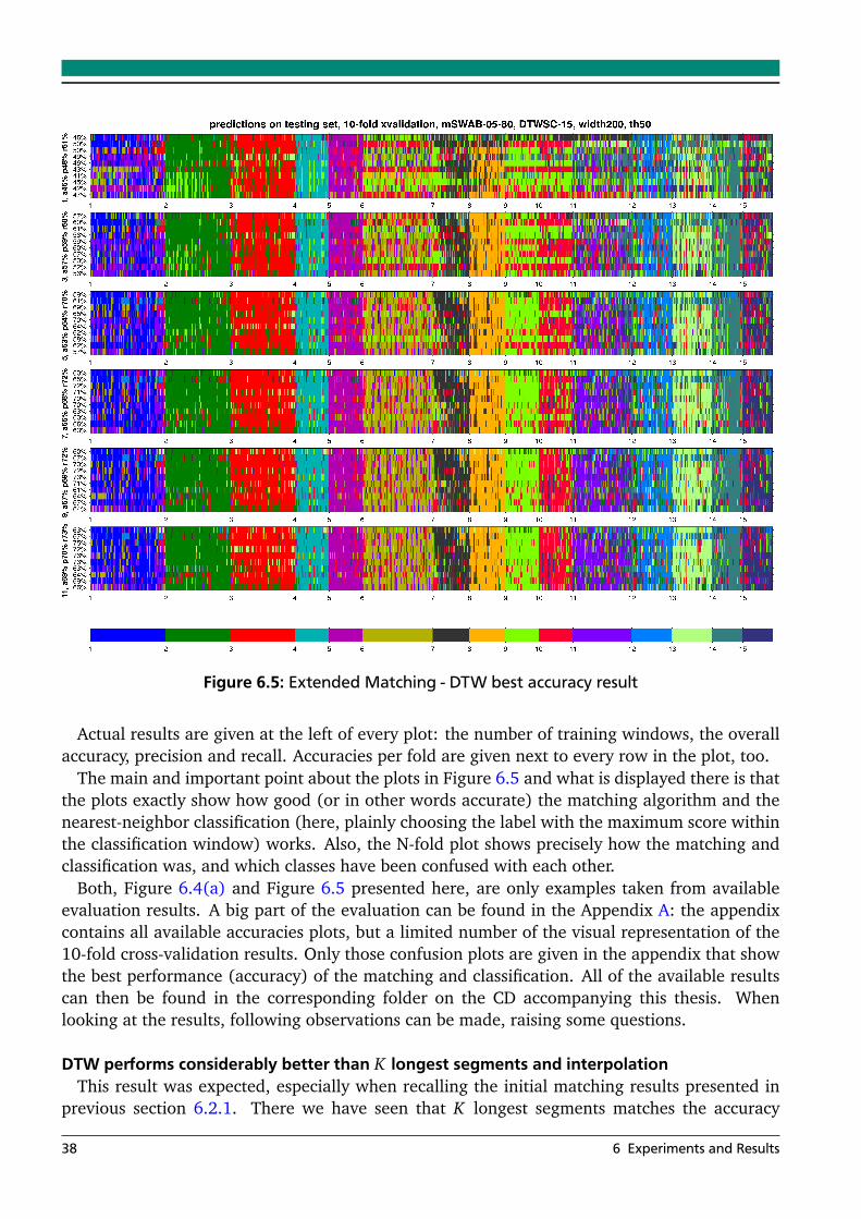
Figure 6.5: Extended Matching - DTW best accuracy result

Actual results are given at the left of every plot: the number of training windows, the overallaccuracy, precision and recall. Accuracies per fold are given next to every row in the plot, too.

The main and important point about the plots in Figure 6.5 and what is displayed there is thatthe plots exactly show how good (or in other words accurate) the matching algorithm and thenearest-neighbor classification (here, plainly choosing the label with the maximum score withinthe classification window) works. Also, the N-fold plot shows precisely how the matching andclassification was, and which classes have been confused with each other.

Both, Figure 6.4(a) and Figure 6.5 presented here, are only examples taken from availableevaluation results. A big part of the evaluation can be found in the Appendix A: the appendixcontains all available accuracies plots, but a limited number of the visual representation of the10-fold cross-validation results. Only those confusion plots are given in the appendix that showthe best performance (accuracy) of the matching and classification. All of the available resultscan then be found in the corresponding folder on the CD accompanying this thesis. Whenlooking at the results, following observations can be made, raising some questions.

DTW performs considerably better than K longest segments and interpolationThis result was expected, especially when recalling the initial matching results presented in

previous section 6.2.1. There we have seen that K longest segments matches the accuracy


performance of DTW in best case, but not in worst case. On average, K longest segments isfaster than, but not as accurate as DTW.

The low accuracy performance of the interpolation approach was expected, too. As theo-rized in section 4.3, the matching of similar but in the time domain slightly stretched motionpatterns would result in high matching distances. The lack of the warping ability, as the out-standing feature of DTW, has therefore a huge negative impact on the accuracy performance ofthe interpolation approach.

Each algorithm has its best accuracy for a different training window size...How and why do the matching algorithms depend on the specific window size? Does the

window size depend on the data set used? Is there a heuristic to find optimal window sizes?

Algorithm Window size

Dynamic time warping 150–300K longest segments 100–150

Interpolation 300

It is interesting to note that DTW performs more or less similarly on different sizes of trainingwindows. This is, as we assume to be most likely, due to its ability to warp data points ofthe query and candidate subsequence, therefore being able to catch the distortions in the timedomain. Thus, the training window size has a not that dominant influence on the accuracyperformance. This behavior holds for the N-fold cross-validation evaluation conducted on theWalk8 as well as Shinson Hapkido data sets, as can be seen in the results in the appendix A.

This behavior does not hold for K longest segments, as there the best accuracy results areachieved with smaller windows. The performance here is related to various parameter values:the training window size (and thus to the number of segments in the query as well as in thecandidate subsequence), to K and also to the cost threshold for mSWAB approximation. Theseare many possible combinations there, so lets have a closer look:

• A small training window of e.g. 100 will have a limited number of segments that areconsidered when selecting the K longest segments for matching. Increasing the trainingwindow size and keeping the K fix to, say 5, will lead to the shape being not sufficientlydescribed by these K longest segments, thus leading to accuracy drop. Please comparethe results displayed in the Figures A.3, A.5 and A.7. Thus, for keeping the accuracyperformance at a high level, when increasing the training window size also K needs to beadjusted accordingly.

• To point out another interesting result, we see that K longest segments performed almostequally well on a fine-grained and coarse-grained approximations (Figures A.5 and A.17)with only slightly better results for the latter. The only mentionable difference lies withthe training window sizes of 50 and 100, where the accuracy for mSWAB-10-80 was at∼10%. This is due to too few segments available in the query and the candidate window.Increasing the training window size for coarse-grained approximation to 150 or more willprovide enough segments to choose upon, thus also resulting in quite good accuracies.

• Also, we want to point out that the best accuracies were achieved with K = 10 and train-ing window size of 150 for both the fine- and coarse-grained approximations, with one


exception only that also has relative low accuracy of 47%, as shown in A.3. The accuracyachieved by K longest segments approach for all the other cases and 11 training windowslies over 50%.

Also, this behavior can not be reproduced for interpolation matching. The maximum ac-curacy is achieved when using a training window size of 300. The accuracy tends to growmonotonously when the training window size is increased starting at 50, achieving the maxi-mum at 300, and then dropping again, as can be seen in Figure A.9 and A.11. This resemblesthe same behaviour as with DTW. Due to the lack of the warping feature, interpolation is notable to reach the high accuracy resutls of DTW.

So, thus we end up with a question, can we come up with a heuristic that will detect theoptimal training window size, depending on the data set, the approximation and matchingalgorithm and their parameters?

Increasing the number of training windows improves the accuracy. What is optimal here?This result is not very surprising, since more training windows capture more motion patterns

that are descriptive for the corresponding training data and thus for the person-activity label.On the other hand, we need to also consider the huge time complexity impact when increasingthe number of segments.

With the evaluation results available we observe that the accuracy improvement steps arehigh when increasing the number of training windows from 1 to 3 or 5. Increasing to 7 or moretraining windows will result in the improvement steps to become much smaller. Since on everystep we add 2 more windows, the computational impact is of a high order ([to be computed]).

This leads us to the question: what is a good number of training windows? Since we need toconsider both the time needed for matching, as well as the accuracy, how shall this trade-off besolved?

Why does interpolation matching approach perform that bad with 10% penalty threshold andmuch better with 20%?

This question is a bit more tricky. We have already discussed out initial observations in section4.3 when introducing the interpolation approach. There we have pointed out that similar butstretched motion patterns tend to result in high matching distance, whereas the distance of onesuch motion pattern to a flat signal containing only few segments might turn out to be lower.By introducing a fix threshold of e.g. 10% deviation in the amount of segments, we try to avoidthese false matches.

It seems that a 10% threshold, as has been tried out during the extended evaluation, is way toorestrictive and therefore results in similar patterns and therefore correct matches to be sortedout during the matching distance computation. Allowing a higher discrepance in the segments’number by increasing the threshold to 20%, we observe the accuracy performance jumping from36% to 54%. Thus, the simple answer to the question why this improvement: by increasing thethreshold we consider more potential close matches.

Still, a fix threshold, as already mentioned, is not an elegant solution. In future work aweighting for the interpolation approach should be considered for implementation.


7 Conclusions and Future Work

In this chapter we give a short summary of the work done during the thesis and what has beenpresented in this report, followed by some ideas for future work directions.

7.1 Summary and Conclusion

What was the thesis and this report all about? The motivation for this work lies in two aims:first, to find a fast, efficient and online approximation technique that would allow to port itsimplementation to a wearable microcontroller-based sensor device, and second, to supportparticipating subjects at their annotating task by providing close matches to selected motionpatterns in real-time. Therefore, this thesis was divided in two parts, one dealing with variousapproximation algorithms and the other with three shape matching techniques.

When we started dealing with approximation of human accelerometer data and its visual pre-sentation to a human, it become obvious very fast that the traditional features such as mean andvariance or the approximation with Discrete Fourier Coefficients does not suit our demands: thelow computational complexity, accuracy of approximation and ease of visualization. By mov-ing on to piecewise linear approximation algorithms, especially its well known representativeSliding Window, we observed promising results. A lot of time then has been spent on finding agood and online PLA algorithm. Going from Sliding Windows over to the Bottom-Up approachshowed us that a more accurate approximation can be achieved. Since Bottom-Up is not online,we had to move on to SWAB, a combination of Bottom-Up and Sliding Windows. This approachis online and gives good approximation of the human accelerometer data, but still can be con-siderably sped up. Our modification, mSWAB, was then proposed and, after various evaluationson different data sets, has been proven to match the approximation accuracy of SWAB whilebeing almost twice as fast on our human accelerometer data sets. mSWAB and the performanceresults comparison with SWAB and Sliding Window were presented to the scientific communityin [26] and [27].

The second part of the thesis was all about finding a fast and accurate shape matching tech-niques to allow us to provide close matches to a selected motion pattern almost in real-time.The first step was to implement and benchmark the state-of-the-art matching algorithm for time-series: dynamic time warping. This algorithm is used throughout the scientific community andprovides a unique feature to optimally warp the data points of two timeseries subsequences andthis way to fix small time distortions. Unfortunately, shape matching with original DTW is of aquadratic time complexity. There are various approaches to bound the warping paths, but stillthe question remains whether there are other shape matching algorithms that are faster and cankeep up with the matching accuracy of DTW. In this thesis two matching algorithms, K longestsegments and interpolation, have been proposed. The first considers the K most descriptive(and in human accelerometer data we assume those are the longest) segments for the queryand matches these against the candidate’ segments computing the euclidean distance. The in-terpolation approach keeps the number of segments and interpolates the missing points on thetwo motion patterns; on these the sum of squared distances is computed and used as similarity

41

measure. The evaluation of these three algorithms was done in two parts, first we comparedDTW and K longest segments. The initial evaluation showed that K longest segments is muchfaster than DTW on a challenging data set: 5 subjects were performing 3 activities – walking,climbing and descending stairs. On the other hand, the accuracy of K longest segments matchedthe one of DTW for some subjects, but was much worse for others. The extended evaluationwas considering all three algorithms and was run using the generic evaluation script and twodata sets. Here we observed that also interpolation greatly outperforms DTW in terms of theexecution time, but due to the lack of the warping feature results in low accuracy.

7.2 Future Work

Heuristic to find motion patterns of interestAn algorithm that is able to find motion patterns should be added, instead of the selection of

the highest variance windows of a fix length (e.g. 250). To achieve this, we need to search foran optimal algorithm. The field of motif discovery needs to be investigated in this context.

Multi-dimensional mSWAB approximationWith the presented mSWAB approximation results at hand, we should consider a multi-

dimensional version of mSWAB, too. The question to answer there is, whether it might beeven better and more efficient than the one-dimensional mSWAB. To answer this question, anew implementation is need. This direction has not been persued due to time (as well asdue to the fact that the traditional SWAB algorithm we based ourselves upon does not have astandard implementation for this), but would be promising especially for the widely used 3Daccelerometers. We expect mSWAB’s slope checking to perform a lot better than SWAB in amulti-dimensional implementation.

Further investigation and testing of SwiftSegThe polynomial approximation, here represented by SwiftSeg, is a promising direction to

investigate. Especially its low runtime on big data sets make it an interesting alternative to PLAalgorithms. On the other hand, the high number of computation steps in its implementationmight turn out to be a show stopper when considering an implementation on a microcontroller-based device. Due to lack of time, only the basic functionality of this algorithm have beenimplemented during this thesis.

Linking the motion patterns to activitiesThis is the next step towards activity recognition. It requires an algorithm that spots the

motion patterns typical for an activity and accumulates this as evidence to give an estima-tion of when what activity was performed, based on solely accelerometer data. This is furtherdown the road, but would complete our approach in fully exploiting every bit of information inacceleration data.

Various ideas on further future workAs always, we suggest to evaluate the algorithms presented in this work on more data sets as

well as with more users. As already mentioned, an adapted – multi-dimensional – implementa-tions of mSWAB is worth closer consideration.

42 7 Conclusions and Future Work

Bibliography

[1] O. Amft, H. Junker, and G. Tröster. Detection of eating and drinking arm gestures usinginertial body-worn sensors. In ISWC 2005: IEEE Proceedings of the Ninth InternationalSymposium on Wearable Computers, pages 160–163, 2005.

[2] E. Fuchs, C. Gruber, T. Reitmaier, and B. Sick. Processing short-term and long-term infor-mation with a combination of polynomial approximation techniques and time-delay neuralnetworks. IEEE Transactions on Neural Networks, 20(9):1450–1462, September 2009.

[3] E. Fuchs, T. Gruber, J. Nitschke, and B. Sick. On-line motif detection in time series withswiftmotif. Pattern Recogn., 42(11):3015–3031, 2009.

[4] E. Fuchs, T. Gruber, J. Nitschke, and B. Sick. On-line segmentation of time series basedon polynomial least-squares approximations. IEEE Transactions On Pattern Analysis AndMachine Intelligence (accepted), 2009.

[5] K. M. Hsiao, G. West, and S. Vedatesh. Online context recognition in mul-tisensor sys-tem using dynamic time warping. In Proceedings of the 2005 International Conference onIntelligent Sensors, Sensor Networks and Information Processing, pages 283–288, 2005.

[6] T. Huynh, U. Blanke, and B. Schiele. Scalable recognition of daily activities with wear-able sensors. In Proceedings of the 3rd International Symposium on Location- and Context-Awareness (LoCA), 2007.

[7] T. Huynh and B. Schiele. Analyzing features for activity recognition. In Proceedings of the2005 joint conference on Smart objects and ambient intelligence: innovative context-awareservices: usages and technologies (sOcEuSAI2005), pages 159–163, Grenoble, France, 2005.ACM Press New York, NY, USA, ACM Press New York, NY, USA.

[8] F. Itakura. Minimum prediction residual principle applied to speech recognition. Acoustics,Speech and Signal Processing, IEEE Transactions on, 23(1):67–72, 1975.

[9] H. Junker. Human Activity and Gesture Spotting with Body-Worn Sensors. PhD thesis, ETHZürich, 2005.

[10] E. J. Keogh, S. Chu, D. Hart, and M. J. Pazzani. An online algorithm for segmenting timeseries. In ICDM ’01: Proceedings of the 2001 IEEE International Conference on Data Mining,pages 289–296, 2001.

[11] K. V. Laerhoven and M. Altmann. Shinson Hapkido data set. http://sites.google.com/a/mis.tu-darmstadt.de/porcupine/datasets/shinson-hapkido-data-set.

[12] K. V. Laerhoven and A. K. Aronsen. Walk8 data set. http://sites.google.com/a/mis.tu-darmstadt.de/porcupine/datasets/walk8-data.

[13] K. V. Laerhoven and E. Berlin. ADay09 data set. http://sites.google.com/a/mis.tu-darmstadt.de/porcupine/datasets/aday09.

43

http://sites.google.com/a/mis.tu-darmstadt.de/porcupine/datasets/shinson-hapkido-data-set

http://sites.google.com/a/mis.tu-darmstadt.de/porcupine/datasets/shinson-hapkido-data-set

http://sites.google.com/a/mis.tu-darmstadt.de/porcupine/datasets/walk8-data

http://sites.google.com/a/mis.tu-darmstadt.de/porcupine/datasets/walk8-data

http://sites.google.com/a/mis.tu-darmstadt.de/porcupine/datasets/aday09

http://sites.google.com/a/mis.tu-darmstadt.de/porcupine/datasets/aday09

[14] D. Lemire. Faster retrieval with a two-pass dynamic-time-warping lower bound. PatternRecogn., 42(9):2169–2180, 2009.

[15] J. Lester, T. Choudhury, and G. Borriello. A practical approach to recognizing physicalactivities. In Pervasive Computing, volume 3968 of Lecture Notes in Computer Science, pages1–16. Springer, May 2006.

[16] J. Lin, E. J. Keogh, L. Wei, and S. Lonardi. Experiencing SAX: a novel symbolic represen-tation of time series. Data Min. Knowl. Discov., 15(2):107–144, 2007.

[17] B. Logan, J. Healey, M. Philipose, E. M. Tapia, and S. S. Intille. A long-term evaluation ofsensing modalities for activity recognition. In Ubicomp, volume 4717 of Lecture Notes inComputer Science, pages 483–500. Springer, 2007.

[18] P. Lukowicz, J. Ward, H. Junker, M. Stager, G. Troster, A. Atrash, and T. Starner. Recog-nizing workshop activity using body worn microphones and accelerometers. In PervasiveComputing, volume 3001 of Lecture Notes in Computer Science, pages 18–32. Springer,2004.

[19] D. Minnen, T. Starner, I. Essa, and C. Isbell. Discovering characteristic actions from on-bodysensor data. In International Symposium on Wearable Computers (ISWC), 2006.

[20] G. Ogris, T. Stiefmeier, P. Lukowicz, and G. Tröster. Using a complex multi-modal on-bodysensor system for activity spotting. In Proceedings of the 12th IEEE International Symposiumon Wearable Computers, pages 55–62, 2008.

[21] L. Rabiner and B.-H. Juang. Fundamentals of speech recognition. Prentice-Hall, Inc., UpperSaddle River, NJ, USA, 1993.

[22] N. Rajpoot and K. Masood. Human gait recognition with 3dwavelets and kernel basedsubspace projections. In Human Activity Recognition and Modeling (HAREM), 2005.

[23] C. Ratanamahatana and E. Keogh. Making time-series classification more accurate usinglearned constraint. In SIAM International Conference on Data Mining, 2004.

[24] H. Sakoe and S. Chiba. Dynamic programming algorithm optimization for spoken wordrecognition. IEEE Transactions on Acoustics, Speech and Signal Processing, 26(1):43–49,1978.

[25] J. Shieh and E. Keogh. iSAX: Indexing and mining terabyte sized time series. In SIGKDD2008, 2008.

[26] K. Van Laerhoven and E. Berlin. When else did this happen? Efficient subsequence repre-sentation and matching for wearable activity data. In Proceedings of the 13th InternationalSymposium on Wearable Computers (ISWC 2009), pages 101–104, Linz, Austria, 2009.

[27] K. Van Laerhoven, E. Berlin, and B. Schiele. Enabling efficient time series analysis for wear-able activity data. In Proceedings of the 8th International Conference on Machine Learningand Applications (ICMLA 2009), page to appear, Miami, FL, USA, 2009. IEEE Press.

[28] J. A. Ward, P. Lukowicz, G. Tröster, and T. E. Starner. Activity recognition of assembly tasksusing body-worn microphones and accelerometers. IEEE Trans. Pattern Anal. Mach. Intell.,28(10):1553–1567, 2006.

44 Bibliography

A Experiment Results

In this appendix, experiment results of N -fold cross-validations on the walking and hapkido datasets are presented. Before moving on to the results, we give a short explanation how to read theplots.

To simplify matters, let us first clarify the terms and abbreviation used in the title of the plotsby looking at this example: [10-fold xvalidation, mSWAB-5-80, DTWSC-15, width50, th50]

abbreviation description

10-fold This is the number of folds used in the cross-validation: N = 10.mSWAB-5-80 The algorithm used to approximate raw training and testing data.

E.g. mSWAB with cost threshold c t = 5 and buffer size bs = 80.Other PLA algorithms can be used, but mSWAB is the algorithm ofchoice for the approximation of human accelerometer data.

DTWSC-15 The algorithm used for shape matching. Here: Dynamic Time Warp-ing that was bounded by the Sakoe-Chiba band of width 15. Otheralgorithms are: K longest segments (KLS-K) with a fixed number ofsegments or Interpolation (IP-p) with a penalty threshold.

width50 This is the width M = 50 of the m non-overlapping training windowswith maximum variance that are used for cross-validation.

th50 This threshold is used in the classification window of fixed width(currently: 500). When voting for a particular activity-person is con-ducted, only the scores (1-distance normalized over the whole data)are considered that lie over 50%. The prediction (the activity-personlabel with the maximum score) is then compared to the actually truelabel, thus building the confusion matrix.

For the evaluation, the parameters in the plot title are kept fix and the number of patterns mused for cross-validation is varied. With m ∈ {1, 3,5, 7,9, 11}, this gives us 6 plots per page. Themeaning of the abbreviations on the y axis of the plots (e.g. 5, a61%, p62%, r71%) are:

abbreviation description

5 this leading digit gives us the number m = 5 of non-overlappingwindows of width M (e.g. M = 50, as given by width50)

a61% overall accuracy of the matching for the given parametersp62% overall precision of the matching for the given parametersr71% overall recall of the matching for the given parameters

Each row in the plot visually represents the classification results for one fold. Additionally tothe overall performance of the classification, accuracy per fold is given.

45

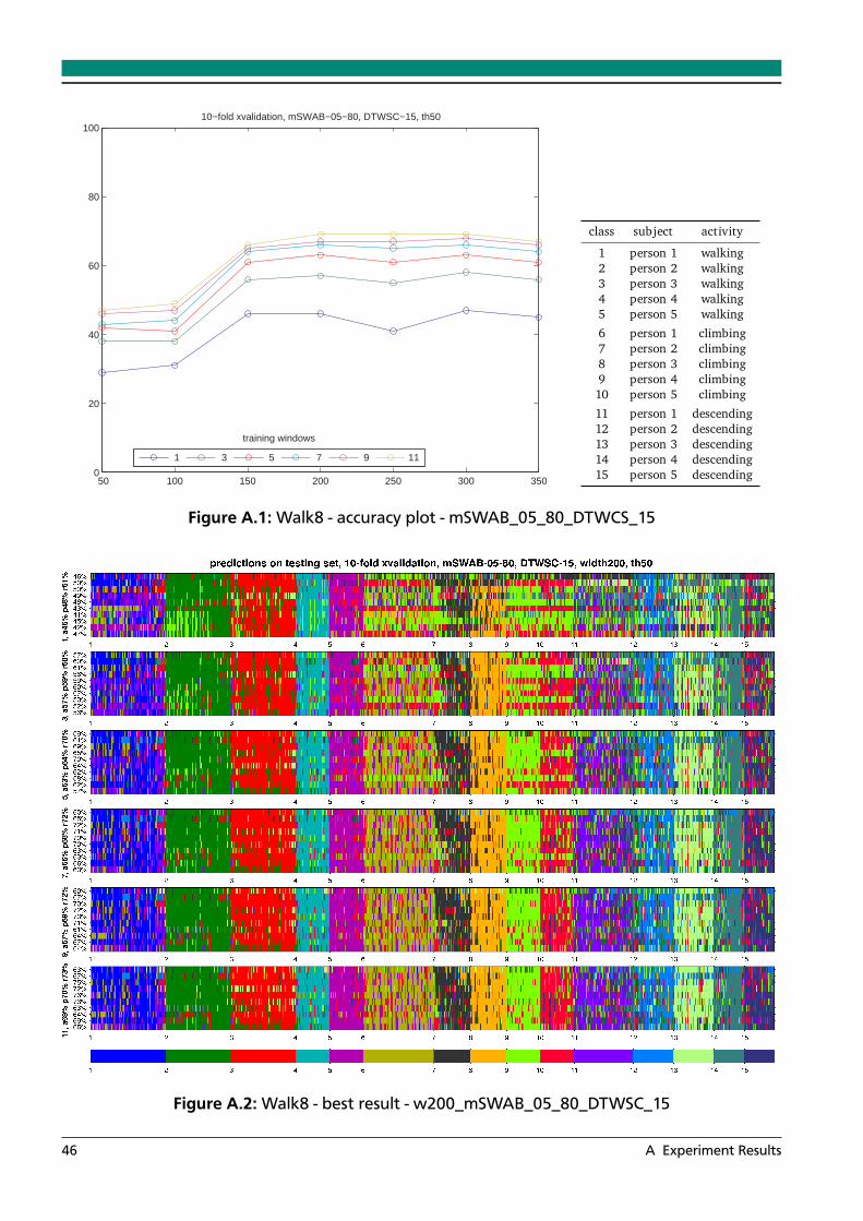
50 100 150 200 250 300 3500

20

40

60

80


1 3 5 7 9 11

training windows





Figure A.1: Walk8 - accuracy plot - mSWAB_05_80_DTWCS_15

Figure A.2: Walk8 - best result - w200_mSWAB_05_80_DTWSC_15

46 A Experiment Results

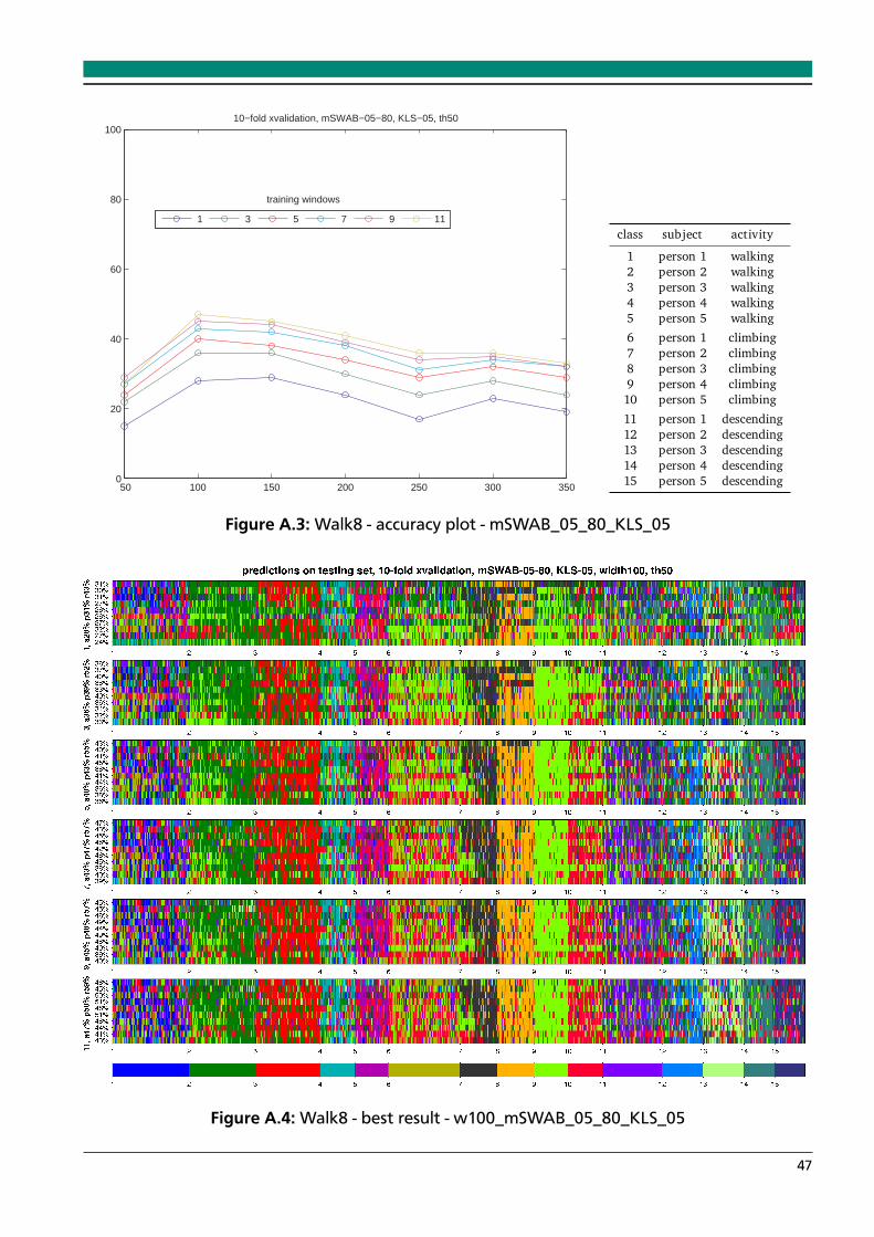
50 100 150 200 250 300 3500

20

40

60

80

10010−fold xvalidation, mSWAB−05−80, KLS−05, th50

1 3 5 7 9 11

training windows





Figure A.3: Walk8 - accuracy plot - mSWAB_05_80_KLS_05

Figure A.4: Walk8 - best result - w100_mSWAB_05_80_KLS_05

47

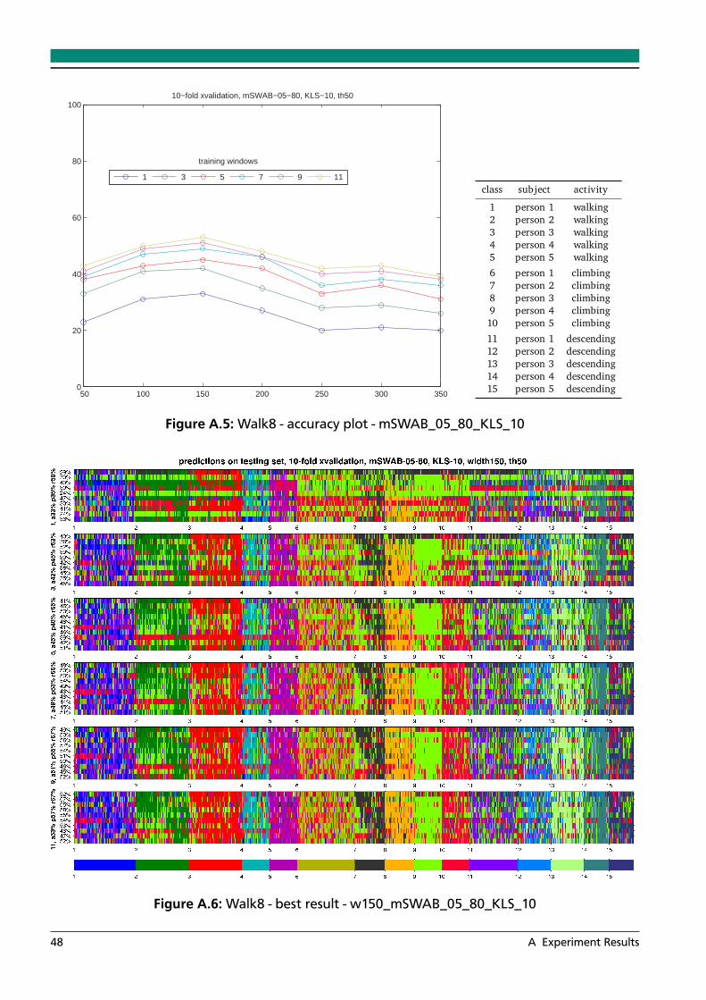
50 100 150 200 250 300 3500

20

40

60

80


1 3 5 7 9 11

training windows








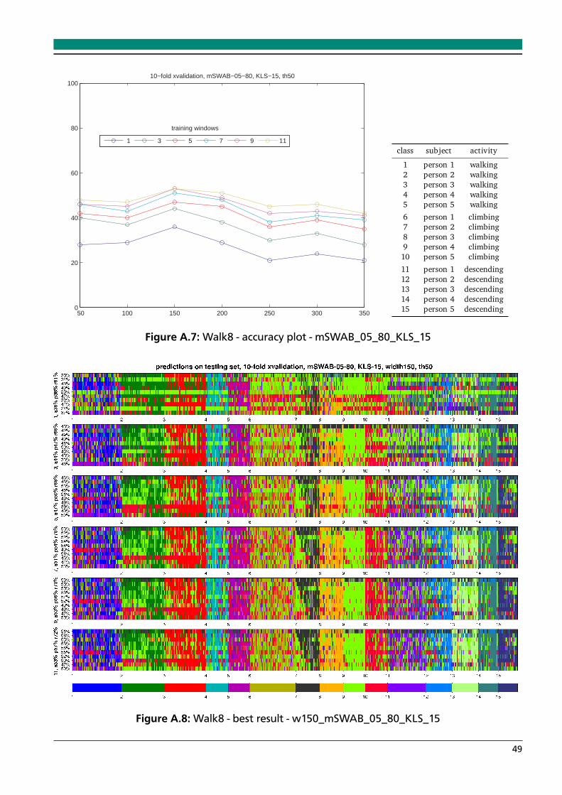
50 100 150 200 250 300 3500

20

40

60

80


1 3 5 7 9 11

training windows







49

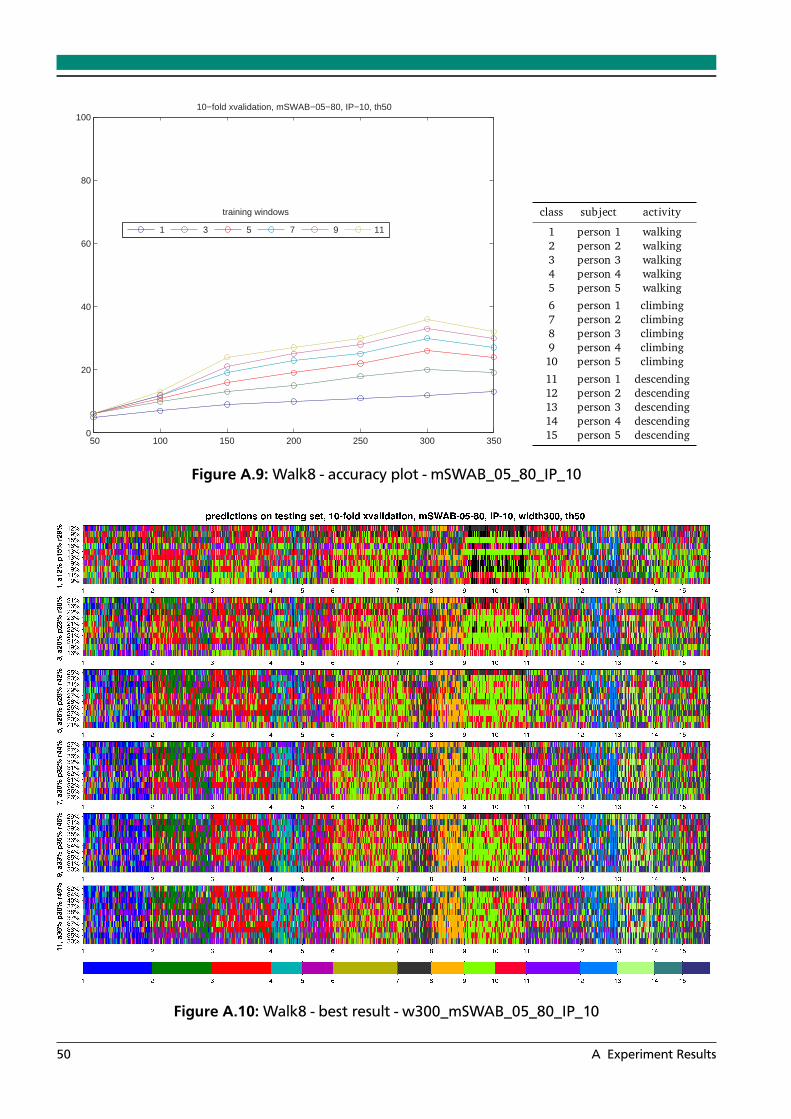
50 100 150 200 250 300 3500

20

40

60

80

10010−fold xvalidation, mSWAB−05−80, IP−10, th50

1 3 5 7 9 11

training windows class subject activity




Figure A.9: Walk8 - accuracy plot - mSWAB_05_80_IP_10

Figure A.10: Walk8 - best result - w300_mSWAB_05_80_IP_10


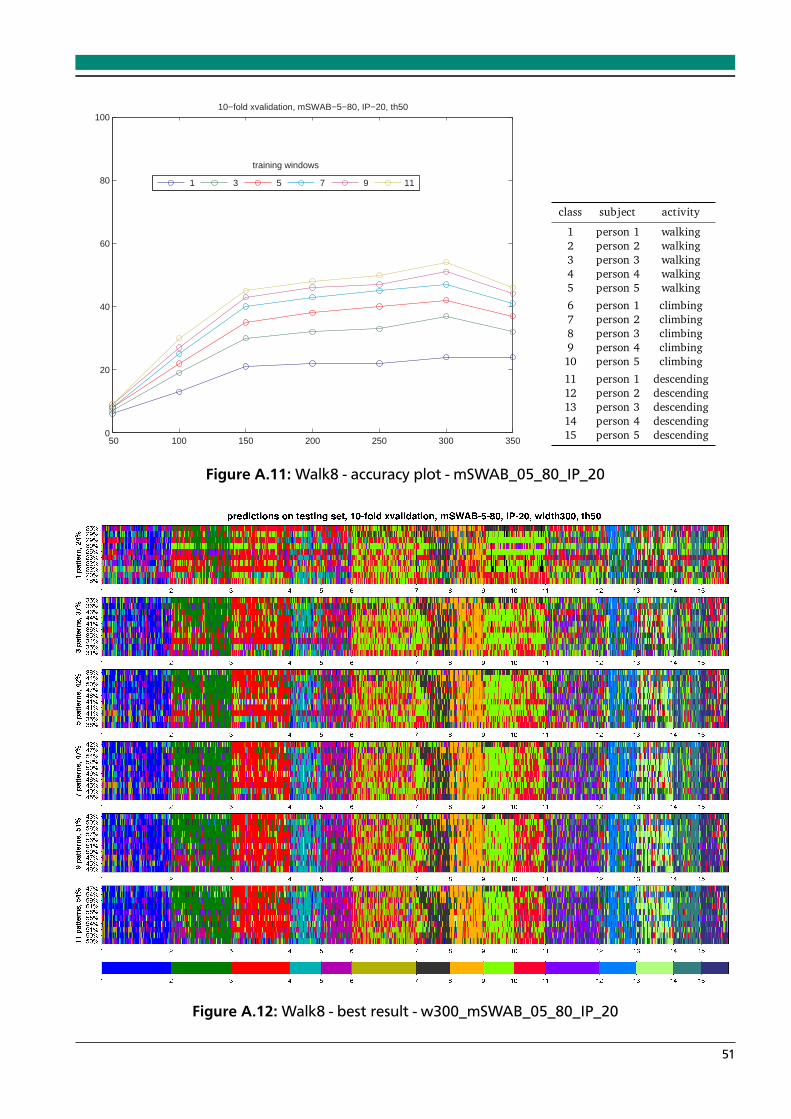
50 100 150 200 250 300 3500

20

40

60

80

10010−fold xvalidation, mSWAB−5−80, IP−20, th50

1 3 5 7 9 11

training windows





Figure A.11: Walk8 - accuracy plot - mSWAB_05_80_IP_20

Figure A.12: Walk8 - best result - w300_mSWAB_05_80_IP_20

51

50 100 150 200 250 300 3500

20

40

60

80


1 3 5 7 9 11

training windows





Figure A.13: Walk8 - accuracy plot - mSWAB_10_80_DTWCS_15

Figure A.14: Walk8 - best result - w300_mSWAB_10_80_DTWSC_15


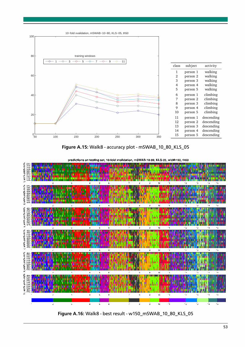
50 100 150 200 250 300 3500

20

40

60

80


1 3 5 7 9 11

training windows







53

50 100 150 200 250 300 3500

20

40

60

80


1 3 5 7 9 11

training windows








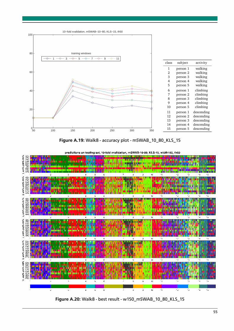
50 100 150 200 250 300 3500

20

40

60

80


1 3 5 7 9 11

training windows







55

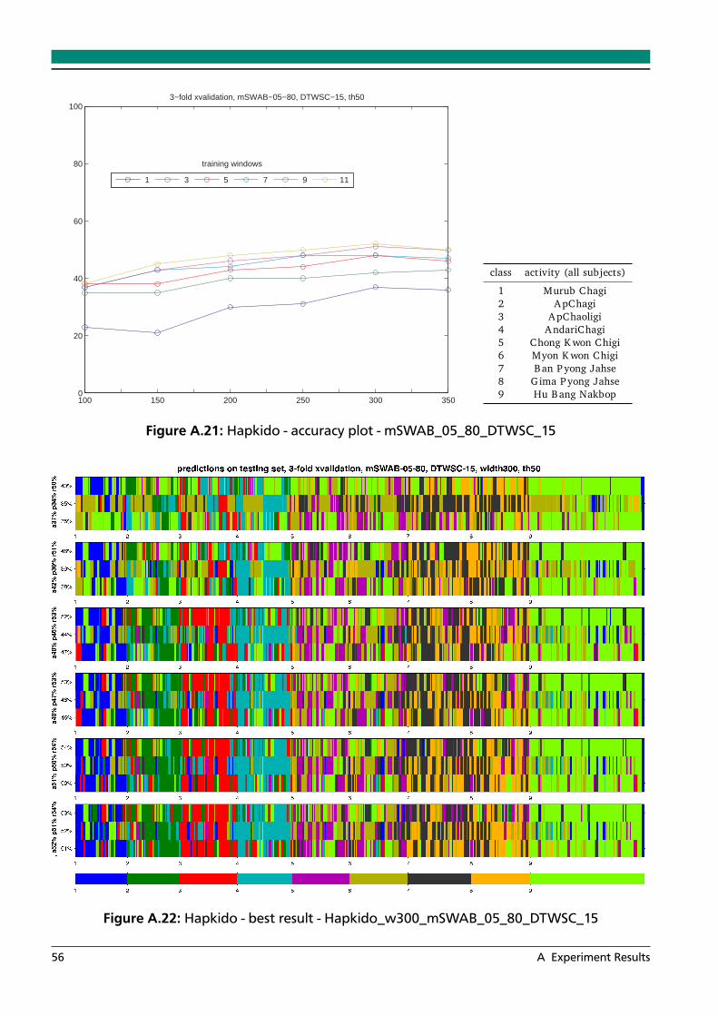
100 150 200 250 300 3500

20

40

60

80


1 3 5 7 9 11

training windows

class activity (all subjects)

1 Murub Chagi2 ApChagi3 ApChaoligi4 AndariChagi5 Chong Kwon Chigi6 Myon Kwon Chigi7 Ban Pyong Jahse8 Gima Pyong Jahse9 Hu Bang Nakbop

Figure A.21: Hapkido - accuracy plot - mSWAB_05_80_DTWSC_15

Figure A.22: Hapkido - best result - Hapkido_w300_mSWAB_05_80_DTWSC_15


100 150 200 250 300 3500

20

40

60

80


1 3 5 7 9 11

training windows

class activity (all subjects)

1 Murub Chagi2 ApChagi3 ApChaoligi4 AndariChagi5 Chong Kwon Chigi6 Myon Kwon Chigi7 Ban Pyong Jahse8 Gima Pyong Jahse9 Hu Bang Nakbop

Figure A.23: Hapkido - accuracy plot - mSWAB_10_80_DTWSC_15

Figure A.24: Hapkido - best result - Hapkido_w300_mSWAB_10_80_DTWSC_15

57

B Time Series GUI and X11 Plots

This appendix presents the GUI prototype that was created during the thesis.As shown in Figure B.1(a), this GUI allows the user to easily approximate raw data files with

PLA algorithms discussed previously (Sliding Windows, SWAB and mSWAB) and adjust theparameters to his liking. After the approximation, or when an already exising approximationfile is avaliable, the approximation segments can be displayed in a X11 plot, as shown in FigureB.1(b). By selecting a pattern of particular interest, as shown in B.1(c), the user is able to findclosest matches using one of the matching algorithms. The resulting closest matches will bedisplayed as shown in B.1(d).

(a) The TimeSeries GUI

(b) Approximated subsequence

(c) Selecting a motion pattern

(d) Closest matches and their matching cost

Figure B.1: A GUI prototype to approximation and matching algorithms discussed in this thesis.The first X11 window plot shows a 3 dimensional accelerometer subsequence. Byselecting a motion pattern of interest, the user can initiate matching and thus searchfor closest matches. These will be displayed in the plot, too.

59

An Empirical Study of Time Series Approximation …Department of Computer Science Multimodal...

Documents

Transcript of An Empirical Study of Time Series Approximation …Department of Computer Science Multimodal...