An Empirical Study of the Impact of Modern Code Review ... · Keywords Code review software quality...
45
Noname manuscript No. (will be inserted by the editor) An Empirical Study of the Impact of Modern Code Review Practices on Software Quality Shane McIntosh · Yasutaka Kamei · Bram Adams · Ahmed E. Hassan Author pre-print copy. The final publication is available at Springer via: http://dx.doi.org/10.1007/s10664-015-9381-9 Abstract Software code review, i.e., the practice of having other team members critique changes to a software system, is a well-established best practice in both open source and proprietary software domains. Prior work has shown that formal code inspections tend to improve the quality of delivered software. However, the for- mal code inspection process mandates strict review criteria (e.g., in-person meetings and reviewer checklists) to ensure a base level of review quality, while the mod- ern, lightweight code reviewing process does not. Although recent work explores the modern code review process, little is known about the relationship between modern code review practices and long-term software quality. Hence, in this paper, we study the relationship between post-release defects (a popular proxy for long-term software quality) and: (1) code review coverage, i.e., the proportion of changes that have been code reviewed, (2) code review participation, i.e., the degree of reviewer involvement in the code review process, and (3) code reviewer expertise, i.e., the level of domain- specific expertise of the code reviewers. Through a case study of the Qt, VTK, and ITK projects, we find that code review coverage, participation, and expertise share a significant link with software quality. Hence, our results empirically confirm the intuition that poorly-reviewed code has a negative impact on software quality in large systems using modern reviewing tools. Shane McIntosh · Ahmed E. Hassan Software Analysis and Intelligence Lab (SAIL) Queen’s University, Canada E-mail: [email protected], [email protected] Yasutaka Kamei Principles of Software Languages group (POSL) Kyushu University, Japan E-mail: [email protected] Bram Adams Lab on Maintenance, Construction, and Intelligence of Software (MCIS) Polytechnique Montr´ eal, Canada E-mail: [email protected]
Transcript of An Empirical Study of the Impact of Modern Code Review ... · Keywords Code review software quality...
Noname manuscript No.(will be inserted by the editor)
An Empirical Study of the Impact of Modern Code ReviewPractices on Software Quality
Shane McIntosh · Yasutaka Kamei · BramAdams · Ahmed E. Hassan
Author pre-print copy. The final publication is available at Springer via:http://dx.doi.org/10.1007/s10664-015-9381-9
Abstract Software code review, i.e., the practice of having other team memberscritique changes to a software system, is a well-established best practice in bothopen source and proprietary software domains. Prior work has shown that formalcode inspections tend to improve the quality of delivered software. However, the for-mal code inspection process mandates strict review criteria (e.g., in-person meetingsand reviewer checklists) to ensure a base level of review quality, while the mod-ern, lightweight code reviewing process does not. Although recent work explores themodern code review process, little is known about the relationship between moderncode review practices and long-term software quality. Hence, in this paper, we studythe relationship between post-release defects (a popular proxy for long-term softwarequality) and: (1) code review coverage, i.e., the proportion of changes that have beencode reviewed, (2) code review participation, i.e., the degree of reviewer involvementin the code review process, and (3) code reviewer expertise, i.e., the level of domain-specific expertise of the code reviewers. Through a case study of the Qt, VTK, andITK projects, we find that code review coverage, participation, and expertise sharea significant link with software quality. Hence, our results empirically confirm theintuition that poorly-reviewed code has a negative impact on software quality in largesystems using modern reviewing tools.
Shane McIntosh · Ahmed E. HassanSoftware Analysis and Intelligence Lab (SAIL)Queen’s University, CanadaE-mail: [email protected], [email protected]
Yasutaka KameiPrinciples of Software Languages group (POSL)Kyushu University, JapanE-mail: [email protected]
Bram AdamsLab on Maintenance, Construction, and Intelligence of Software (MCIS)Polytechnique Montreal, CanadaE-mail: [email protected]

2 Shane McIntosh et al.
Keywords Code review · software quality
1 Introduction
Software code reviews are a well-documented best practice for software projects.In his seminal work, Fagan (1976) notes that formal design and code inspectionswith in-person meetings reduced the number of errors that are detected during thetesting phase in small development teams. Rigby and Bird (2013) find that the moderncode review processes that are adopted through a variety of reviewing mediums (e.g.,mailing lists or the Gerrit web application1) tend to converge on a lightweight variantof the formal code inspections of the past, where the focus has shifted from defect-hunting to collaborative problem-solving. Nonetheless, Bacchelli and Bird (2013)find that one of the main motivations of modern code review still is to improve thequality of a change to the software.
Prior work indicates that formal design and code inspections can be an effec-tive means of identifying defects so that they can be fixed early in the developmentcycle (Fagan, 1976). Tanaka et al. (1995) suggest that code inspections should beapplied meticulously to each code change. Kemerer and Paulk (2009) indicate thatstudent submissions tend to improve in quality when design and code inspectionsare introduced. However, there is little evidence of the long-term impact that modern,lightweight code review processes (which lack the rigid structure of code inspections)have on software quality in large systems.
In particular, to truly improve the quality of a set of proposed changes, review-ers must carefully consider the potential implications of the changes and engage ina discussion with the author. Under the formal code inspection model, time is allo-cated explicitly for the preparation and execution of in-person meetings, where thereviewers and the author discuss the proposed code changes (Fagan, 1976). Further-more, reviewers are encouraged to follow a checklist to ensure that a base level ofreview quality is achieved. However, in the modern reviewing process, such strict re-viewing criteria are not mandated (Rigby and Storey, 2011), and hence, reviews maynot foster a sufficient amount of discussion between author and reviewers. Indeed,Microsoft developers complain that reviews often focus on minor logic errors ratherthan discussing deeper design issues (Bacchelli and Bird, 2013).
We hypothesize that a modern code review process that neglects to review a largeproportion of code changes, that suffers from low reviewer participation, or that doesnot involve subject matter experts will likely have a negative impact on softwarequality. In other words:
If a large proportion of the code changes that are integrated duringdevelopment are either: (1) omitted from the code review process(low review coverage), (2) have lax code review involvement (lowreview participation), or (3) do not include a subject matter expert(low expertise), then defect-prone code will permeate through to thereleased software product.
1https://code.google.com/p/gerrit/
An Empirical Study of the Impact of Modern Code Review Practices on Software Quality 3
Tools that support the modern code reviewing process, such as Gerrit, explic-itly link changes to a software system recorded in a Version Control System (VCS)to their respective code review. In this paper, we leverage these links to calculatecode review coverage, participation, and expertise metrics, and add them to statisti-cal regression models that are built to explain the incidence of post-release defects(i.e., defects in official releases of a software product), which is a popular proxy forsoftware quality (Bird et al., 2011; Hassan, 2009; Kamei et al., 2013; Mockus andWeiss, 2000; Nagappan and Ball, 2007). Rather than using these models for defectprediction, we analyze the impact that code review metrics have on the models whilecontrolling for a variety of metrics that are known to be good explainers of softwarequality. Through a case study of four releases of the large Qt, VTK, and ITK opensource systems, we address the following three research questions:
(RQ1) Is there a relationship between code review coverage and post-release de-fects?We find that review coverage is negatively associated with the incidence ofpost-release defects in three of the four studied releases. However, it onlyprovides a significant amount of explanatory power to two of the four stud-ied releases, suggesting that review coverage alone does not guarantee a lowincidence rate of post-release defects.
(RQ2) Is there a relationship between code review participation and post-releasedefects?We find that the incidence of post-release defects is also associated with de-veloper participation in code review. Review discussion metrics play a statis-tically significant role in the explanatory power of all of the studied systems.
(RQ3) Is there a relationship between code reviewer expertise and post-releasedefects?Our models indicate that components with many changes that do not involvea subject matter expert in the authoring or reviewing process tend to be proneto post-release defects.
This paper is an extended version of our earlier work (McIntosh et al., 2014). Weextend the prior work to:
– Use contemporary regression modelling techniques (Harrell Jr., 2002) (Section 3)that:1. Relax the requirement of a linear relationship between post-release defect
counts and explanatory variables, which enables a more accurate fit of thedata.
2. Filter away redundant variables, i.e., explanatory variables that may not behighly correlated with other explanatory variables, but do not provide a signalthat is distinct with respect to the other explanatory variables.
3. Allow us to analyze the stability of our models.– Study the impact of reviewer expertise on software quality (RQ3).– Include two additional review participation metrics (RQ2) and one additional re-
view expertise metric (RQ3) that are not threshold-dependent, i.e., discussionspeed (normalized by churn), discussion length (normalized by churn), and voterexpertise.

4 Shane McIntosh et al.
Fig. 1 An example Gerrit code review.
1.1 Paper Organization
The remainder of the paper is organized as follows. Section 2 describes the Gerrit-driven code review process that is used by the studied systems. Section 3 describesthe design of our case study, while Section 4 presents the results of our three researchquestions. Section 5 discloses the threats to the validity of our study. Section 6 surveysrelated work. Finally, Section 7 draws conclusions.
2 Gerrit Code Review
Gerrit1 is a modern code review tool that facilitates a traceable code review processfor git-based software projects (Bettenburg et al., 2014). It tightly integrates withtest automation and code integration tools. Authors upload patches, i.e., collectionsof proposed changes to a software system, to a Gerrit server. The set of reviewers areeither: (1) invited by the author, (2) appointed automatically based on their expertisewith the modified system components, or (3) self-selected by broadcasting a reviewrequest to a mailing list. Figure 1 shows an example code review in Gerrit that wasuploaded on December 1st, 2012. Below, we use this figure to illustrate the role thatreviewers and verifiers play in a code review.
2.1 Reviewers
Reviewers are responsible for critiquing the changes proposed within the patch byleaving comments for the author to address or discuss. The author can reply to com-ments or address them by producing a new revision of the patch for the reviewers toconsider.
Reviewers can also give the changes proposed by a patch revision a score, whichindicates: (1) agreement or disagreement with the proposed changes (positive or neg-

An Empirical Study of the Impact of Modern Code Review Practices on Software Quality 5
ative value), and (2) their level of confidence (1 or 2). The second column of thebottom-most table in Figure 1 shows that the change has been reviewed and the re-viewer is in agreement with it (+). The text in the fourth column (“Looks good to me,approved”) is displayed when the reviewer has a confidence level of two.
2.2 Verifiers
In addition to reviewers, verifiers are also invited to evaluate patches in the Gerritsystem. Verifiers execute tests to ensure that patches: (1) truly fix the defect or addthe feature that the authors claim to, and (2) do not cause regression of system func-tionality. Similar to reviewers, verifiers can provide comments to describe verificationissues that they have encountered during testing. Furthermore, verifiers can also pro-vide a score of 1 to indicate successful verification, and -1 to indicate failure.
While team personnel can act as verifiers, so too can Continuous Integration (CI)tools that automatically build and test patches. For example, CI build and testingjobs can be automatically launched each time a new review request or patch revisionis uploaded to Gerrit. The reports generated by these CI jobs can be automaticallyappended as a verification report to the code review discussion. The third column ofthe bottom-most table in Figure 1 shows that the “Qt Sanity Bot” has successfullyverified the change.
2.3 Automated integration
Gerrit allows teams to codify code review and verification criteria that must be sat-isfied before changes are integrated into upstream VCS repositories. For example,a team policy may specify that at least one reviewer and one verifier should pro-vide positive scores prior to integration. Once the criteria are satisfied, patches areautomatically integrated into upstream repositories. The “Merged” status shown inthe upper-most table of Figure 1 indicates that the proposed changes have been inte-grated.
3 Case Study Design
In this section, we present our rationale for selecting our research questions, describethe studied systems, and present our data extraction and analysis approaches.
3.1 Research Questions
Broadly speaking, the main goal of this paper is to study whether lax involvement thatmay creep into the modern, lightweight code review process has a negative impacton software quality. We focus on three aspects of modern code review practices thatwe believe may have an impact on software quality (i.e., coverage, participation, and

6 Shane McIntosh et al.
Table 1 Overview of the studied systems. Those to the left of the double line satisfy our criteria foranalysis.
Qt VTK ITK Android LibreOfficeVersion 5.0 5.1 5.10 4.3 4.0.4 4.0Tag name v5.0.0 v5.1.0 v5.10.0 v4.3.0 4.0.4 4.0.0Size (LOC) 5,560,317 5,187,788 1,921,850 1,123,614 18,247,796 4,789,039Components w/ defects 254 187 15 24 - -Components total 1,339 1,337 170 218 - -Defective rate 19% 14% 9% 11% - -Commits w/ reviews 10,003 6,795 554 344 1,727 1,679Commits total 10,163 7,106 1,431 352 80,398 11,988Review rate 98% 96% 39% 98% 2% 14%# Authors 435 422 55 41 - -# Reviewers 358 348 45 37 - -
expertise). We leave the exploration of other aspects of code review practices to futurework.
In order to evaluate our conjecture about lax code review practices, we formulatethe following three research questions:
(RQ1) Is there a relationship between code review coverage and post-release de-fects?Tanaka et al. (1995) suggest that a software team should meticulously re-view each change to the source code to ensure that quality standards are met.In more recent work, Kemerer and Paulk (2009) find that design and codeinspections have a measurable impact on the defect density of student sub-missions at the Software Engineering Institute (SEI). While these findingssuggest that there is a relationship between code review coverage and soft-ware quality, the scale of such a relationship has remained largely unexploredin large software systems using modern code reviewing tools.
(RQ2) Is there a relationship between code review participation and post-releasedefects?To truly have an impact on software quality, developers must invest in thecode reviewing process. In other words, if developers are simply approvingcode changes without discussing them, the code review process likely pro-vides little value. Hence, we set out to study the relationship between devel-oper participation in code reviews and software quality.
(RQ3) Is there a relationship between code reviewer expertise and post-releasedefects?Changes produced by novice developers are more likely to introduce defectsthan those produced by subject matter experts (Mockus and Weiss, 2000).However, a change produced by a novice can be improved by soliciting feed-back from subject matter experts during the code review process. Hence, weset out to study whether changes that are developed by personnel who lacksubject matter expertise have an impact on software quality if they are notreviewed by a subject matter expert.

An Empirical Study of the Impact of Modern Code Review Practices on Software Quality 7
3.2 Studied Systems
In order to address our research questions, we perform a case study on large, suc-cessful, and rapidly-evolving open source systems with globally distributed develop-ment teams. In selecting the subject systems, we identified two important criteria thatneeded to be satisfied:
Criterion 1: Reviewing Policy – We want to study systems that have made a seri-ous investment in code reviewing. Hence, we only study systems where a largenumber of the integrated patches have been reviewed.
Criterion 2: Traceability – The code review process for a subject system must betraceable, i.e., it should be reasonably straightforward to connect a large propor-tion of the integrated patches to the associated code reviews. Without a traceablecode review process, review coverage and participation metrics cannot be calcu-lated, and hence, we cannot perform our analysis.
To satisfy the traceability criterion, we focus on software systems that use theGerrit code review tool. We began our study with five subject systems, however afterpreprocessing the data, we found that only 2% of Android and 14% of LibreOfficechanges could be linked to reviews, so both systems had to be removed from ouranalysis (Criterion 1).
Table 1 shows that the Qt, VTK, and ITK systems satisfied our criteria for analysis.Qt is a cross-platform application framework whose development is supported by theDigia corporation, however welcomes contributions from the community-at-large.2
The Visualization ToolKit (VTK) is used to generate 3D computer graphics and pro-cess images.3 The Insight segmentation and registration ToolKit (ITK) provides asuite of tools for in-depth image analysis.4
3.3 Data Extraction
In order to evaluate the impact that code review coverage, participation, and exper-tise have on software quality, we extract code review data from the Gerrit reviewdatabases of the studied systems, and link the review data to the integrated patchesrecorded in the corresponding VCSs.
Figure 2 shows that our data extraction approach is broken down into three steps:(1) extract review data from the Gerrit review database, (2) extract Gerrit change IDsfrom the VCS commits, and (3) calculate version control metrics. We briefly describeeach step of our approach below.
3.3.1 Extract reviews
Our analysis is based on the Qt code reviews dataset collected by Hamasaki et al.(2013). The dataset describes each review, the involved personnel, and the details
2http://qt.digia.com/3http://vtk.org/4http://itk.org/

8 Shane McIntosh et al.
GerritReviews
Version Control System
(1)Extract Reviews
(2)Extract Change ID
(3)Calculate Version Control Metrics
ReviewDatabase
CodeDatabase
Change Id Componentdata
Fig. 2 Overview of our data extraction approach.
of the review discussions. We expand the dataset to include the reviews from theVTK and ITK systems, as well as those reviews that occurred during the more recentdevelopment cycle of Qt 5.1. To do so, we use a modified version of the GerritMinerscripts provided by Mukadam et al. (2013).
3.3.2 Extract change ID
Each review in a Gerrit database is uniquely identified by an alpha-numeric hash codecalled a change ID. When a review has satisfied project-specific criteria, it is auto-matically integrated into the upstream VCS (cf. Section 2). For traceability purposes,the commit message of the automatically integrated patch contains the change ID.We extract the change ID from commit messages in order to automatically connectpatches in the VCS with the associated code review process data. To facilitate futurework, we have made the code and review databases available online.5
3.3.3 Calculate version control metrics
Prior work has found that several types of metrics have a relationship with defect-proneness. Since we aim to investigate the impact that code reviewing has on defect-proneness, we control for the three most common families of metrics that are knownto have a relationship with defect-proneness (Shihab et al., 2011; Hassan, 2009; Birdet al., 2011). Table 2 provides a brief description and the motivating rationale foreach of the studied baseline metrics. Similar to prior work (Nagappan et al., 2006;Bird et al., 2011), we measure each metric at the component (i.e., directory) level.
We focus our analysis on the development activity on the release branches ofeach studied system, i.e., activity that: (1) occurred on the main development branchbefore the release branch was cut, (2) occurred on the release branch itself, and(3) originated on other branches, but has been merged into the release branch.Prior to a release, the integration of changes on a release branch is more strictly
5http://sailhome.cs.queensu.ca/replication/reviewing_quality_ext/

An Empirical Study of the Impact of Modern Code Review Practices on Software Quality 9
Table 2 A taxonomy of the considered baseline component metrics.
Metric Description Rationale
Prod
uct Size Number of lines of
code.Large components are more likely to bedefect-prone (Koru et al., 2009).
Complexity The McCabe cyclo-matic complexity.
More complex components are likely moredefect-prone (Menzies et al., 2002).
Proc
ess
Priordefects
Number of defectsfixed prior to release.
Defects may linger in components that wererecently defective (Graves et al., 2000).
Churn Sum of added and re-moved lines of code.
Components that have undergone a lot ofchange are likely defect-prone (Nagappanand Ball, 2005, 2007).
Change en-tropy
A measure of the dis-tribution of changesamong files.
Components where changes are spreadamong several files are likely defect-prone(Hassan, 2009).
Hum
anFa
ctor
s
Totalauthors
Number of uniqueauthors.
Components with many unique authorslikely lack strong ownership, which in turnmay lead to more defects (Bird et al., 2011;Graves et al., 2000).
Minor au-thors
Number of uniqueauthors who havecontributed less than5% of the changes.
Developers who make few changes to a com-ponent may lack the expertise required toperform the change in a defect-free manner(Bird et al., 2011). Hence, components withmany minor contributors are likely moredefect-prone.
Majorauthors
Number of uniqueauthors who havecontributed at least5% of the changes.
Similarly, components with a large num-ber of major contributors, i.e., those withcomponent-specific expertise, are less likelyto be defect-prone (Bird et al., 2011).
Authorownership
The proportion ofchanges contributedby the author whomade the mostchanges.
Components with a highly active componentowner are less likely to be defect-prone (Birdet al., 2011).
controlled than a typical development branch to ensure that only the appropriately-triaged changes will appear in the upcoming release. Moreover, changes that land ona release branch after a release are also strictly controlled to ensure that only high-priority fixes land in maintenance releases. In other words, the changes that we studycorrespond to the development and maintenance of official software releases.
To determine whether a change fixes a defect, we search the VCS commit mes-sages for co-occurrences of defect identifiers with keywords like “bug”, “fix”, “de-fect”, or “patch”. A similar approach was used to determine defect-fixing and defect-inducing changes in other work (Mockus and Votta, 2000; Hassan, 2008; Kim et al.,2008; Kamei et al., 2013). Similar to prior work (Kamei et al., 2010), we define post-release defects as those with fixes recorded in the six-month period after the releasedate.
Product metrics. Product metrics measure the source code of a system at the time ofa release. It is common practice to preserve the released versions of the source codeof a software system in the VCS using tags. In order to calculate product metrics

10 Shane McIntosh et al.
for the studied releases, we first extract the released versions of the source code by“checking out” those tags from the VCS.
We measure the size and complexity of each component (i.e., directory) as de-scribed below. We measure the size of a component by aggregating the number oflines of code in each of its files. We use McCabe’s cyclomatic complexity (McCabe,1976) (calculated using Scitools Understand6) to measure the complexity of a file. Tomeasure the complexity of a component, we take the sum of the complexity of eachfile within it. Finally, since complexity measures are often highly correlated with size,we divide the complexity of each component by its size to reduce the influence of sizeon complexity measures. A similar approach was used in prior work (Kamei et al.,2010).Process metrics. Process metrics measure the change activity that occurred duringthe development of a new release. Process metrics must be calculated with respect toa time period and a development branch. Again, similar to prior work (Kamei et al.,2010), we measure process metrics using the six-month period prior to each releasedate on the release branch.
We use prior defects, churn, and change entropy to measure the change process.We count the number of defects fixed in a component prior to a release by usingthe same pattern-based approach that we use to identify post-release defects. Churnmeasures the total number of lines added to and removed from a component priorto release. As suggested by Nagappan and Ball (2005), we divide the churn of eachcomponent by its size. Change entropy measures how the complexity of a changeprocess is distributed across files (Hassan, 2009). We measure the change entropy ofeach component individually, i.e., we calculate how evenly spread out the changes toa component’s files before the release are for each component in isolation. Similarto Hassan (2009), we use the Shannon (1948) entropy normalized by the maximumentropy for a component c as described below:
H(c) =−
n∑
k=1(pk ∗ log2 pk)
log2n, (1)
where n is the number of files in component c, and pk is the proportion of thechanges to c that occur in file k. Such a normalized entropy allows one to comparethe H(c) between components of different sizes with different numbers of files.Human factors. Human factor metrics measure developer expertise and code own-ership. Similar to process metrics, human factor metrics must also be calculated withrespect to a time period. We again adopt the six-month period prior to each releasedate as the window for metric calculation.
Table 2 shows that we adopt the suite of ownership metrics proposed by Birdet al. (2011). Total authors is the number of authors that contribute to a component.Minor authors is the number of authors that contribute fewer than 5% of the commitsto a component. Major authors is the number of authors that contribute at least 5% ofthe commits to a component. Author ownership is the proportion of commits that themost active contributor to a component has made.
6http://www.scitools.com/documents/metricsList.php?#Cyclomatic

An Empirical Study of the Impact of Modern Code Review Practices on Software Quality 11
Component data
Explanatory variables
Post-releasedefect count
(MC-3)Correlation
analysis
(MC-4)Redundancy
analysis
(MC-1)Estimate
budget for degrees of freedom
(MC-2)Normality
adjustment
(MC-5)Allocate
degrees of freedom
(MC-6)Fit
regression model
(MA-1)Assessment
of model stability
(MA-2)Estimate power of
explanatory variables
(MA-3)Examine
variables in relation to outcome
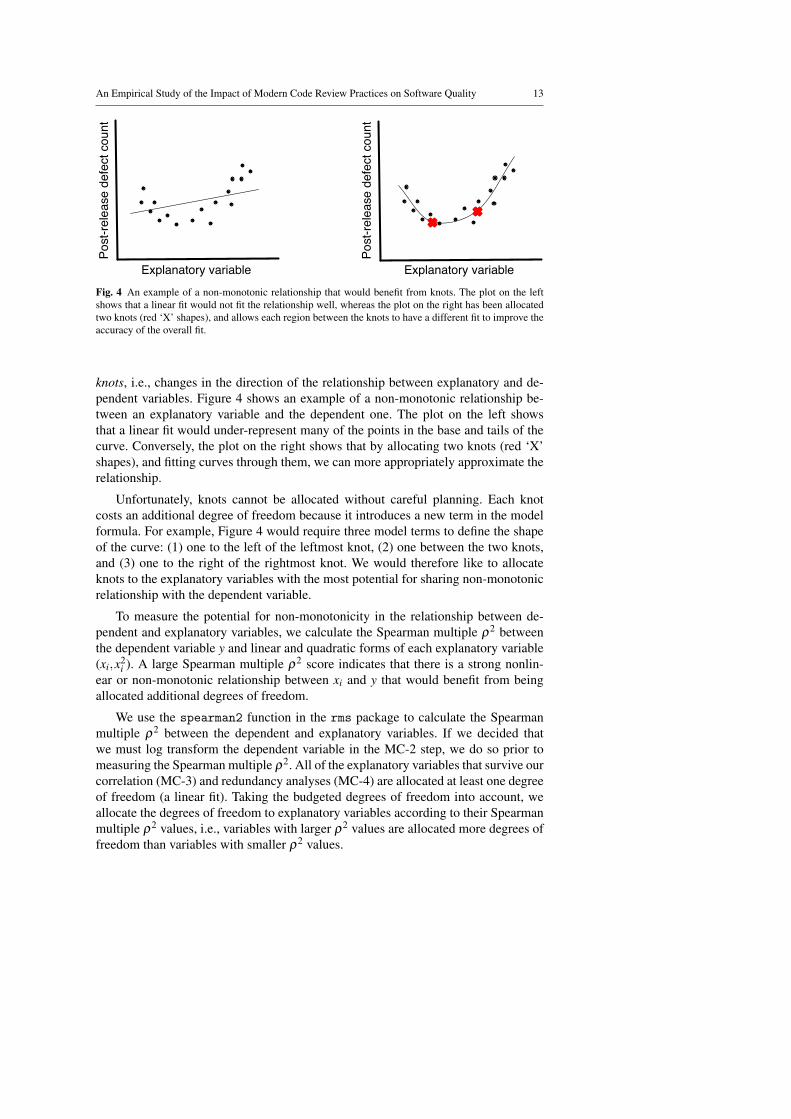
Fig. 3 Overview of our Model Construction (MC) and Model Analysis (MA) approach.
3.4 Model Construction
We build regression models to explain the incidence of post-release defects detectedin the components of the studied systems. A regression model fits a curve of the formy = β0 +β1x1 +β2x2 + · · ·+βnxn to the data, where y is the dependent variable andeach xi is an explanatory variable. In our models, the dependent variable is the post-release defect count and the explanatory variables are the set of metrics outlined inTables 2 and 3.
We adopt the model construction and analysis approach of Harrell Jr. (2002).These techniques relax linearity assumptions between explanatory and dependentvariables, allowing nonlinear relationships to be modelled more accurately, whilebeing mindful of the potential for overfitting, i.e., constructing a model that is toospecialized for the dataset on which the model was trained that it would not apply toother datasets. We use the R implementation (R Core Team, 2013) of the techniquesdescribed by Harrell Jr. (2002) provided by the rms package (Harrell Jr., 2014).
Figure 3 provides an overview of the six steps in our model construction ap-proach. Figure 14 in Appendix A provides the R code for each of these steps. Wedescribe each step in the approach below.
(MC-1) Estimate Budget for Degrees of Freedom
When constructing explanatory or predictive models, a critical concern is that of over-fitting. An overfit model will exaggerate or dismiss relationships between the depen-dent and explanatory variables based on characteristics of the dataset from which itwas built.
Overfitting may creep into models that use more degrees of freedom (e.g., ex-planatory variables) than a dataset can support. Hence, it is pragmatic to calculatea budget of degrees of freedom that a dataset can support before attempting to fit amodel. As suggested by Harrell Jr. et al. (1984, 1985), we budget n
15 degrees of free-dom for our defect models, where n is the number of rows (i.e., components) in thedataset.

12 Shane McIntosh et al.
(MC-2) Normality Adjustment
We fit our regression models using the Ordinary Least Squares (OLS) technique us-ing the ols function provided by the rms package. OLS expects that the dependentvariable is normally distributed. Since software engineering data is often skewed, weanalyze the distribution of post-release defect counts in each studied system prior tofitting our models. If we find that the distribution is skewed, we apply a log trans-formation [ln(x+ 1)] to lessen the skew, and better fit the assumptions of the OLStechnique.
(MC-3) Correlation Analysis
Prior to building our models, we check for explanatory variables that are highly cor-related with one another using Spearman rank correlation tests (ρ). We choose a rankcorrelation instead of other types of correlation (e.g., Pearson) because rank correla-tion is resilient to data that is not normally distributed.
We use a variable clustering analysis to construct a hierarchical overview of thecorrelation among the explanatory variables (Sarle, 1990). For sub-hierarchies of ex-planatory variables with correlation |ρ| > 0.7, we select only one variable from thesub-hierarchy for inclusion in our models.
(MC-4) Redundancy Analysis
Correlation analysis reduces collinearity among the explanatory variables, but it maynot detect all of the redundant variables, i.e., variables that do not have a uniquesignal from the other explanatory variables. Redundant variables in an explanatorymodel will interfere with each other, distorting the modelled relationship betweenthe explanatory and dependent variables. We, therefore, remove redundant variablesprior to constructing our defect models.
In order to detect redundant variables, we fit preliminary models that explain eachexplanatory variable using the other explanatory variables. We use the R2 value of thepreliminary models to measure how well each explanatory variable is explained bythe other explanatory variables.
We use the implementation of this approach provided by the redun function inthe rms package. The function builds preliminary models for each explanatory vari-able. The explanatory variable that is most well-explained by the other explanatoryvariables is iteratively dropped until either: (1) no preliminary model achieves an R2
above a cutoff threshold (for this paper, we use the default threshold of 0.9), or (2) re-moving a variable would make a previously dropped variable no longer explainable,i.e., its preliminary model will no longer achieve an R2 exceeding the threshold.
(MC-5) Allocate Degrees of Freedom
After removing highly correlated and redundant variables, we must decide how tospend our budgeted degrees of freedom most effectively. Specifically, we are mostconcerned with identifying the explanatory variables that would benefit most from
An Empirical Study of the Impact of Modern Code Review Practices on Software Quality 13Po
st-re
leas
e de
fect
cou
nt
Post
-rele
ase
defe
ct c
ount
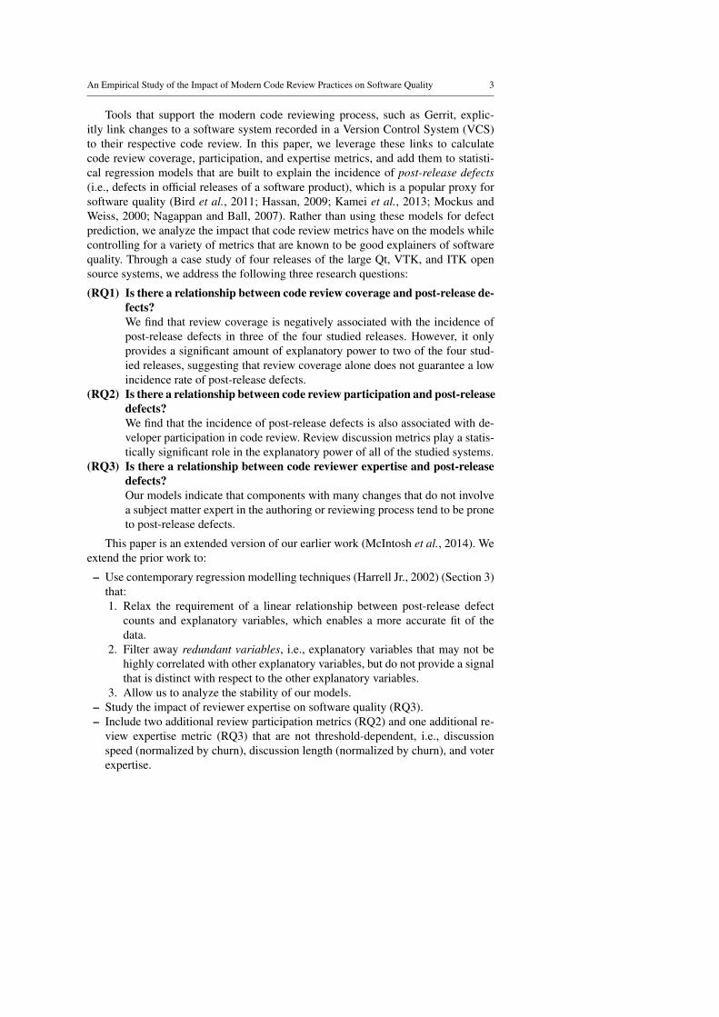
Explanatory variable Explanatory variableFig. 4 An example of a non-monotonic relationship that would benefit from knots. The plot on the leftshows that a linear fit would not fit the relationship well, whereas the plot on the right has been allocatedtwo knots (red ‘X’ shapes), and allows each region between the knots to have a different fit to improve theaccuracy of the overall fit.
knots, i.e., changes in the direction of the relationship between explanatory and de-pendent variables. Figure 4 shows an example of a non-monotonic relationship be-tween an explanatory variable and the dependent one. The plot on the left showsthat a linear fit would under-represent many of the points in the base and tails of thecurve. Conversely, the plot on the right shows that by allocating two knots (red ‘X’shapes), and fitting curves through them, we can more appropriately approximate therelationship.
Unfortunately, knots cannot be allocated without careful planning. Each knotcosts an additional degree of freedom because it introduces a new term in the modelformula. For example, Figure 4 would require three model terms to define the shapeof the curve: (1) one to the left of the leftmost knot, (2) one between the two knots,and (3) one to the right of the rightmost knot. We would therefore like to allocateknots to the explanatory variables with the most potential for sharing non-monotonicrelationship with the dependent variable.
To measure the potential for non-monotonicity in the relationship between de-pendent and explanatory variables, we calculate the Spearman multiple ρ2 betweenthe dependent variable y and linear and quadratic forms of each explanatory variable(xi,x2
i ). A large Spearman multiple ρ2 score indicates that there is a strong nonlin-ear or non-monotonic relationship between xi and y that would benefit from beingallocated additional degrees of freedom.
We use the spearman2 function in the rms package to calculate the Spearmanmultiple ρ2 between the dependent and explanatory variables. If we decided thatwe must log transform the dependent variable in the MC-2 step, we do so prior tomeasuring the Spearman multiple ρ2. All of the explanatory variables that survive ourcorrelation (MC-3) and redundancy analyses (MC-4) are allocated at least one degreeof freedom (a linear fit). Taking the budgeted degrees of freedom into account, weallocate the degrees of freedom to explanatory variables according to their Spearmanmultiple ρ2 values, i.e., variables with larger ρ2 values are allocated more degrees offreedom than variables with smaller ρ2 values.

14 Shane McIntosh et al.
(MC-6) Fit Regression Model
Finally, after selecting appropriate explanatory variables, log transforming the depen-dent variable (if necessary according to MC-2), and allocating budgeted degrees offreedom to the explanatory variables that will yield the most benefit from them, we fitour regression models to the data. We use restricted cubic splines to fit the budgetednumber of knots to the explanatory variables that we allocated additional degrees offreedom to. Cubic splines fit cubic forms of an explanatory variable in order to jointhe different model terms. However, in an unrestricted form, cubic splines tend to fitpoorly in the tails, i.e., before the first knot and after the last one, due to the curlingnature of a cubic curve. Restricted cubic splines force the tails of the relationship tobe linear, and tend to better fit nonlinear relationships (Harrell Jr., 2002).
3.5 Model Analysis
After building regression models, we evaluate the goodness of fit using the AdjustedR2 (Hastie et al., 2009). Unlike the unadjusted R2, the adjusted R2 accounts for thebias of introducing additional degrees of freedom by penalizing models for each de-gree of freedom spent.
As shown in Figure 3, we perform three model analysis steps in order to: (1) studythe stability of our models, (2) estimate the impact of each explanatory variable onmodel performance, and (3) study the relationship between each explanatory variablewhile controlling for the others. Figure 15 in Appendix A provides the R code foreach of these steps. We describe each model analysis step below.
(MA-1) Assessment of Model Stability
While the adjusted R2 of the model gives an impression of how well the model has fitthe dataset, it may overestimate the performance of the model if it is overfit. We takeperformance overestimation into account by subtracting the bootstrap-calculated op-timism (Efron, 1986) from initial adjusted R2 estimates. The optimism of the adjustedR2 is calculated as follows:
1. From the original dataset with n components, select a bootstrap sample, i.e., anew sample of n components with replacement.
2. In the bootstrap sample, fit a model using the same allocation of degrees of free-dom as was used in the original dataset.
3. Apply the model built from the bootstrap sample on the bootstrap and originaldatasets, calculating the adjusted R2 in each.
4. The optimism is the difference in the adjusted R2 of the bootstrap sample and theoriginal sample.
The above process is repeated 1,000 times and the average (mean) optimism iscalculated. Finally, we obtain the optimism-reduced adjusted R2 by subtracting theaverage optimism from the original adjusted R2. The smaller the optimism values,the more stable that the original model fit is.
An Empirical Study of the Impact of Modern Code Review Practices on Software Quality 15
Unlike k-fold cross-validation, the model fit that is validated using the abovebootstrap-derived technique is the one fit using the entire dataset. k-fold cross-validationsplits the data into k equal parts, using k−1 parts for fitting the model, setting aside1 fold for testing. The process is repeated k times, using a different part for testingeach time. Notice, however, that models are fit using k− 1 folds (i.e., a subset) ofthe dataset. Models fit using the full dataset are not directly tested when using k-foldcross-validation.
(MA-2) Estimate Power of Explanatory Variables
We would like to estimate the impact that each explanatory variable has on our modelperformance. In our prior work (McIntosh et al., 2014), we evaluated the impact ofeach explanatory variable using the χ2 maximum likelihood tests of a “drop one” ap-proach (Chambers and Hastie, 1992). This test measures the impact of an explanatoryvariable on a model by measuring the difference in the performance of models builtusing: (1) all explanatory variables (the full model), and (2) all explanatory variablesexcept for the one under test (the dropped model). A χ2 test is applied to the resultingvalues to detect whether each explanatory variable improves model performance to astatistically significant degree.
However, in this paper, explanatory variables that have been allocated severaldegrees of freedom are represented with several model terms instead of just one. Tocontrol for the effect of multiple terms, we jointly test the set of explanatory variablemodel terms for each variable using Wald χ2 maximum likelihood (a.k.a., “chunk”)tests. The larger the Wald χ2 value, the larger the impact that a particular explanatoryvariable has on a model’s performance. We report both the raw Wald χ2 value and itssignificance level according to its p-value.
(MA-3) Examine Explanatory Variables in Relation to the Outcome
Finally, we would like to study the relationship that each modelled reviewing metricshares with the post-release defect count. While the coefficients of the model terms inlinear models can give a general impression of the impact that an explanatory variablehas on the outcome, each explanatory variable in our models may be represented byseveral model terms. In order to account for the impact of all of the model termsassociated with an explanatory variable, we plot the change in the estimated numberof post-release defects against the change in each reviewing metric while holdingthe other explanatory variables constant at their median values using the Predict
function in the rms package (Harrell Jr., 2014). The plot will follow the relationship asit changes directions at knot locations (cf. MC-6). Furthermore, change in estimatedvalue approximates the impact on software quality that the accompanying change inthe reviewing metric will have. The plots also show the 95% confidence intervalscalculated based on the 1,000 previously executed bootstrap iterations (cf. MA-1).

16 Shane McIntosh et al.
Table 3 A taxonomy of the considered code review metrics.
Metric Description Rationale
Cov
erag
e(R
Q1)
Proportion of re-viewed changes
The proportion of changesthat have been reviewed inthe past.
Since code review will likely catch defects,components where changes are most oftenreviewed are less likely to contain defects.
Proportion of re-viewed churn
The proportion of churnthat has been reviewed inthe past.
Despite the defect-inducing nature of codechurn, code review should have a preventa-tive impact on defect-proneness. Hence, weexpect that the larger the proportion of codechurn that has been reviewed, the less defectprone a module will be.
Part
icip
atio
n(R
Q2)
Number of self-approved changes
The proportion of changesto a component that areonly approved for integra-tion by the original author.
By submitting a review request, the originalauthor already believes that the code is readyfor integration. Hence, changes that are onlyapproved by the original author have essen-tially not been reviewed.
Number ofhastily-reviewedchanges
The proportion of changesthat are approved for in-tegration at a rate that isfaster than 200 lines perhour.
Prior work has shown that when develop-ers review more than 200 lines of code perhour, they are more likely to let lower qual-ity source code slip through (Kemerer andPaulk, 2009). Hence, components with manychanges that are approved at a rate fasterthan 200 lines per hour are more likely to bedefect-prone.
Number ofchanges withoutdiscussion
The proportion of changesto a component that are notdiscussed.
Components with many changes that are ap-proved for integration without critical dis-cussion are likely to be defect-prone.
Typical reviewwindow∗
The length of time be-tween the creation of a re-view request and its finalapproval for integration,normalized by the size ofthe change (churn).
Components with shorter review windowsmay not be spending enough time carefullyanalyzing the implications of a change, andhence may be more defect-prone.
Typical discus-sion length∗
The length of the reviewdiscussion (i.e., # non-automated comments),normalized by the size ofthe change (churn).
Components with many short review discus-sions may not be deriving value from the re-view process, and hence may be more defect-prone.
Exp
ertis
e(R
Q3)
Number ofchanges that donot involve asubject matterexpert∗
The proportion of changesto a component that are notauthored by nor reviewedby a subject matter expert,i.e., a major author.
Components with many changes that do notincorporate a subject matter expert are morelikely to be defect-prone.
Typical voterexpertise∗
The percentage of priorchanges to a componentthat each voter has eitherauthored or voted on.
Components with a high degree of voter ex-pertise are likely less defect-prone.
∗New metric that did not appear in the earlier version of this paper (McIntosh et al., 2014).
4 Case Study Results
In this section, we present the results of our case study with respect to our threeresearch questions. For each question, we discuss: (a) the metrics that we use to mea-sure the reviewing property, (b) our model construction procedure, and (c) the modelanalysis results.

An Empirical Study of the Impact of Modern Code Review Practices on Software Quality 17
Table 4 Descriptive statistics of the studied review coverage metrics.
Qt VTK ITK5.0 5.1 5.10 4.3
Rev
’dch
ange
s Minimum 0.86 0.00 0.00 0.001st Quartile. 1.00 1.00 0.00 1.00
Median 1.00 1.00 0.00 1.00Mean 0.99 0.98 0.27 0.99
3rd Quartile 1.00 1.00 0.50 1.00Maximum 1.00 1.00 1.00 1.00
Rev
’dch
urn
Minimum 0.50 0.00 0.00 0.001st Quartile. 1.00 1.00 0.00 1.00
Median 1.00 1.00 0.00 1.00Mean 0.99 0.98 0.15 0.99
3rd Quartile 1.00 1.00 0.06 1.00Maximum 1.00 1.00 1.00 1.00
(RQ1) Is there a relationship between code review coverage and post-releasedefects?
Intuitively, one would hope that higher rates of code review coverage will lead tofewer incidences of post-release defects. To investigate this intuition, we use the codereview coverage metrics described in Table 3 in regression models with the baselinemetrics of Table 2.
(RQ1-a) Coverage metrics
Table 4 provides descriptive statistics of the studied review coverage metrics. Theproportion of reviewed changes is the proportion of changes committed to a compo-nent that are associated with code reviews. Similarly, proportion of reviewed churnis the proportion of the churn of a component that is associated with code reviews.For this research question, we set both the proportion of reviewed changes and theproportion of reviewed churn to 1 for components that have not changed during thepre-release time period.
(RQ1-b) Model construction
In this section, we describe the outcome of the model construction steps outlined inFigure 3.(MC-1) Estimate budget of degrees of freedom. Table 5 shows that our data cansupport between 11 ( 170
15 in VTK) and 89 ( 1,33915 in Qt 5.0) degrees of freedom. We
can therefore apply knots more liberally to the explanatory variables in the larger Qtdatasets than in the smaller VTK and ITK ones.(MC-2) Normality adjustment. Analysis of the post-release defect counts of thestudied systems reveals that the values are right-skewed in the larger Qt datasets. Tocounter the skew, we log-transform the post-release defect counts in the Qt datasets.

18 Shane McIntosh et al.
Table 5 Review coverage model statistics (RQ1).
Qt VTK ITK5.0 5.1 5.10 4.3
Adjusted R2 0.64 0.67 0.39 0.44Optimism-reduced adjusted R2 0.62 0.65 0.20 0.22
Wald χ2 2,360∗∗∗ 2,715∗∗∗ 118∗∗∗ 177∗∗∗Budgeted Degrees of Freedom 89 89 11 14
Degrees of Freedom Spent 17 24 9 9
Overall Nonlinear Overall Nonlinear Overall Nonlinear Overall Nonlinear
Size D.F. 4 3 4 3 1 - 1 -χ2 85∗∗∗ 57∗∗∗ 78∗∗∗ 73∗∗∗ 4∗ 15∗∗∗
Complexity D.F. 2 1 2 1 1 - 1 -χ2 7∗ 5∗ 7∗ 7∗ 1◦ < 1◦
Prior defects D.F. 2 1 2 1 2 1 3 2χ2 48∗∗∗ 32∗∗∗ 81∗∗∗ 13∗∗∗ 106∗∗∗ 84∗∗∗ 51∗∗∗ 26∗∗∗
Churn D.F. 1 - 1 - 1 - 1 -χ2 < 1◦ < 1◦ < 1◦ < 1◦
Change entropy D.F. 2 1 4 3 1 - †χ2 11∗∗ 6∗ 34∗∗∗ 30∗∗∗ < 1◦
Total authors D.F. 3 2 † 1 - †χ2 64∗∗∗ 13∗∗∗ 52∗∗∗
Minor authors D.F. ‡ 4 3 ‡ 1 -χ2 55∗∗∗ 40∗∗∗ 25∗∗∗
Major authors D.F. † † † †χ2
Author ownership D.F. 2 1 3 2 1 - 1 -χ2 4◦ 2◦ 4◦ 4◦ 3◦ < 1◦
Reviewed changes D.F. 1 - 4 3 1 - 1 -χ2 1◦ 84∗∗∗ 83∗∗∗ 12∗∗∗ < 1◦
Reviewed churn D.F. † † † †χ2
Discarded during:† Variable clustering analysis (|ρ| ≥ 0.7)‡ Redundant variable analysis (R2 ≥ 0.9)
Statistical significance of explanatory power according to Wald χ2 likelihood ratio test:◦ p≥ 0.05; ∗ p < 0.05; ∗∗ p < 0.01; ∗∗∗ p < 0.001
- Nonlinear degrees of freedom not allocated
On the other hand, the skew is not large enough to be of concern in the smaller VTKand ITK datasets, so we do not apply a transformation to those projects.(MC-3) Correlation analysis. Figure 5 shows the hierarchically clustered Spearmanρ values in the Qt 5.0 dataset. The solid horizontal lines indicate the correlation valueof the two metrics that are connected by the vertical branches that descend from it.The gray dashed line indicates our cutoff value (|ρ|= 0.7). Similar correlation valueswere observed in the other studied systems. To conserve space, we provide onlineaccess to the figures for the other studied systems.7
Analysis of the clustered variable correlations reveals that the proportion of re-viewed churn is too highly correlated with the proportion of reviewed changes toinclude both metrics. Similarly, the number of major authors is too highly correlatedwith the total number of authors. We selected the proportion of reviewed changesand the total number of authors for our models because they are the simpler of themetric pairs to compute. For the sake of completeness, we analyzed models that use
7http://sailhome.cs.queensu.ca/replication/reviewing_quality_ext/

An Empirical Study of the Impact of Modern Code Review Practices on Software Quality 19
Siz
e
Chu
rn Ent
ropy
Aut
hor
owne
rshi
p
Rev
iew
ed c
hang
es
Rev
iew
ed c
hurn
Prio
r de
fect
s
Min
or a
utho
rs
Com
plex
ity
Tota
l aut
hors
Maj
or a
utho
rs
1.0
0.8
0.6
0.4
0.2
0.0
Spe
arm
an ρ
Fig. 5 Hierarchical clustering of variables according to Spearman’s |ρ| in Qt 5.0 (RQ1).
the proportion of reviewed churn instead of the proportion of reviewed changes, aswell as models that use the number of major authors instead of the total number ofauthors, and found that neither change of metric had a discernible impact on modelperformance.(MC-4) Redundancy analysis. Table 5 shows that the number of minor authors is aredundant variable in the Qt 5.0 and VTK datasets. The number of minor authors iswell-explained by the other metrics (R2
Qt5.0 = 0.99, R2VTK = 0.98). Since this metric
is not likely to add additional explanatory power, we exclude it from these models.(MC-5) Allocate degrees of freedom. Figure 6 shows the Spearman multiple ρ2
of the post-release defect count with each explanatory variable in Qt 5.0. Variablesthat show larger Spearman multiple ρ2 values have more potential for sharing a non-monotonic relationship with the post-release defect count, and hence, would benefitmost from additional degrees of freedom. To conserve space, we only show the Spear-man multiple ρ2 figure for the Qt 5.0 system, and provide the figures for the otherstudied systems online.8
By observing the rough clustering of variables according to the Spearman multi-ple ρ2 values, we split the explanatory variables of Figure 6 into three groups. The
8http://sailhome.cs.queensu.ca/replication/reviewing_quality_ext/

20 Shane McIntosh et al.
Prior defects
Total authors
Size
Change entropy
Author ownership
Complexity
Churn
Reviewed changes
N df
1339 2
1339 2
1339 2
1339 2
1339 2
1339 2
1339 2
1339 2●
●
●
●
●
●
●
●
0.00 0.05 0.10 0.15 0.20 0.25 0.30 0.35
Spearman ρ2 Response : Post − release defect count
Adjusted ρ2
Fig. 6 Dotplot of the Spearman multiple ρ2 of each explanatory variable and the post-release defect countin Qt 5.0. Larger values indicate a more potential for non-monotonic relationship (RQ1).
first group contains the number of prior defects, the total number of authors, and thecomponent size, and has the largest potential for non-monotonicity. A second groupcontains the change entropy, author ownership, and complexity metrics, which alsohave some potential for non-monotonicity. The last group contains the churn and theproportion of reviewed changes.
We allocate a maximum of five knots to one explanatory variable to avoid over-fitting its relationship with the post-release defect count (Harrell Jr., 2002). Since wehave a large budget of degrees of freedom for the Qt 5.0 dataset, we allocate fiveknots to the variables in the first group, three to the variables in the second group,and no knots to the variables in the last group (i.e., fit a linear relationship). A similarprocess was used to allocate the degrees of freedom in the other Qt release.
In the studied VTK and ITK releases, we need allocate degrees of freedom morestringently in order to avoid exceeding the budget. Thus, we only provide additionaldegrees of freedom to the explanatory variable with the largest Spearman multiple ρ2
– the number of prior bugs.
(RQ1-c) Model Analysis
In this section, we describe the outcome of our model analysis outlined in Figure 3.(MA-1) Assessment of model stability. Table 5 shows that our defect models achievean adjusted R2 between 0.39 (VTK) and 0.67 (Qt 5.1). However, since these valuesare calculated using the same data that the models were fit with, they are inherentlyoptimistic (Efron, 1986). Hence, we use the bootstrap technique with 1,000 iterationsto calculate the optimism-reduced adjusted R2.
Our results show that the fit of the Qt models is very stable, only having an ad-justed R2 optimism of 0.02. On the other hand, our VTK and ITK models are less sta-
An Empirical Study of the Impact of Modern Code Review Practices on Software Quality 21
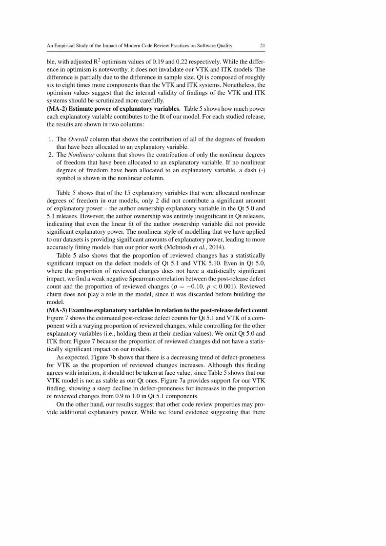
ble, with adjusted R2 optimism values of 0.19 and 0.22 respectively. While the differ-ence in optimism is noteworthy, it does not invalidate our VTK and ITK models. Thedifference is partially due to the difference in sample size. Qt is composed of roughlysix to eight times more components than the VTK and ITK systems. Nonetheless, theoptimism values suggest that the internal validity of findings of the VTK and ITKsystems should be scrutinized more carefully.(MA-2) Estimate power of explanatory variables. Table 5 shows how much powereach explanatory variable contributes to the fit of our model. For each studied release,the results are shown in two columns:
1. The Overall column that shows the contribution of all of the degrees of freedomthat have been allocated to an explanatory variable.
2. The Nonlinear column that shows the contribution of only the nonlinear degreesof freedom that have been allocated to an explanatory variable. If no nonlineardegrees of freedom have been allocated to an explanatory variable, a dash (-)symbol is shown in the nonlinear column.
Table 5 shows that of the 15 explanatory variables that were allocated nonlineardegrees of freedom in our models, only 2 did not contribute a significant amountof explanatory power – the author ownership explanatory variable in the Qt 5.0 and5.1 releases. However, the author ownership was entirely insignificant in Qt releases,indicating that even the linear fit of the author ownership variable did not providesignificant explanatory power. The nonlinear style of modelling that we have appliedto our datasets is providing significant amounts of explanatory power, leading to moreaccurately fitting models than our prior work (McIntosh et al., 2014).
Table 5 also shows that the proportion of reviewed changes has a statisticallysignificant impact on the defect models of Qt 5.1 and VTK 5.10. Even in Qt 5.0,where the proportion of reviewed changes does not have a statistically significantimpact, we find a weak negative Spearman correlation between the post-release defectcount and the proportion of reviewed changes (ρ = −0.10, p < 0.001). Reviewedchurn does not play a role in the model, since it was discarded before building themodel.(MA-3) Examine explanatory variables in relation to the post-release defect count.Figure 7 shows the estimated post-release defect counts for Qt 5.1 and VTK of a com-ponent with a varying proportion of reviewed changes, while controlling for the otherexplanatory variables (i.e., holding them at their median values). We omit Qt 5.0 andITK from Figure 7 because the proportion of reviewed changes did not have a statis-tically significant impact on our models.
As expected, Figure 7b shows that there is a decreasing trend of defect-pronenessfor VTK as the proportion of reviewed changes increases. Although this findingagrees with intuition, it should not be taken at face value, since Table 5 shows that ourVTK model is not as stable as our Qt ones. Figure 7a provides support for our VTKfinding, showing a steep decline in defect-proneness for increases in the proportionof reviewed changes from 0.9 to 1.0 in Qt 5.1 components.
On the other hand, our results suggest that other code review properties may pro-vide additional explanatory power. While we found evidence suggesting that there

22 Shane McIntosh et al.
Proportion of reviewed changes
Pos
t−re
leas
e de
fect
cou
nt
0.0
0.5
1.0
0.0 0.2 0.4 0.6 0.8 1.0
(a) Qt 5.1
Proportion of reviewed changes
Pos
t−re
leas
e de
fect
cou
nt
−2.0
−1.5
−1.0
−0.5
0.0
0.5
0.0 0.2 0.4 0.6 0.8 1.0
(b) VTK
Fig. 7 The estimated count of post-release defects in a typical component for various proportions of re-viewed changes. The blue line indicates the values of our model fit on the original data, while the grey areashows the 95% confidence interval based on models fit to 1,000 bootstrap samples.
is a decreasing trend in defect-proneness as the proportion of reviewed changes ap-proaches 1.0 in Qt 5.1, Figure 7a also indicates that there is an increasing trend indefect-proneness as Qt 5.1 components increase the proportion of reviewed changesfrom 0 to 0.9. This range of values is accompanied by a broadening of the confi-dence interval, suggesting that there is less data supporting this area of the curve. Wefind that indeed, of the 1,337 investigated Qt 5.1 components, only 41 (3%) of themhave a proportion of reviewed changes below 0.9. Nonetheless, the increasing trendin defect-proneness is suggestive of a more complex relationship between review-ing quality and defect-proneness than the proportion of reviewed changes alone cancapture.
In addition, while large proportions of reviewed changes are associated with com-ponents of higher software quality in two of the four studied releases, the metric doesnot provide a statistically significant amount of explanatory power in the other twostudied releases. To gain a richer perspective about the relationship between code re-view coverage and software quality, we manually inspect the ten Qt 5.0 componentswith the most post-release defects.
We find that the Qt 5.0 components with many post-release defects indeed tend tohave lower proportions of reviewed changes. This is especially true for the collectionof nine components that make up the QtSerialPort subsystem, where the propor-tion of reviewed changes does not exceed 0.1. Initial development of the QtSerialPortsubsystem began during Qt 4.x, prior to the introduction of Gerrit to the Qt develop-ment process. Many foundational features of the subsystem were introduced in anincubation area of the Qt development tree, where reviewing policies are more lax.Hence, much of the QtSerialPort code was likely not code reviewed, which mayhave lead to the inflation in post-release defect counts.

An Empirical Study of the Impact of Modern Code Review Practices on Software Quality 23
Yet, there are components with a proportion of reviewed changes of 1 that stillhave post-release defects. Although only 7% of the VTK components with post-release defects (1/15) have a proportion of reviewed changes of 1, 87% (222/254),70% (131/187), and 83% (20/24) of Qt 5.0, Qt 5.1, and ITK components respectivelyhave a proportion of reviewed changes of 1. We further investigate with one-tailedMann-Whitney U tests (α = 0.05) comparing the incidence of post-release defectsin components with a proportion of reviewed changes of 1 to those components withproportions of reviewed change below 1. Test results indicate that Qt 5.1 is the onlystudied release where the incidence of post-release defects in components with pro-portions of reviewed changes of 1 is significantly less than the incidence of post-release defects in components with proportions lower than 1 (p < 2.2× 10⁻¹⁶). Inthe other systems, the difference is not significant (p > 0.05), suggesting that thereis more to the relationship between code review and software quality than coveragealone can explain.
Although high values of review coverage are negatively associated with softwarequality in two of the four defect models, several defect-prone components havehigh coverage rates, suggesting that other properties of the code review processare at play.
(RQ2) Is there a relationship between code review participation and post-releasedefects?
As discussed in RQ1, even components with a proportion of reviewed changes of 1(i.e., 100% code review coverage) can still be defect-prone. We suggest that a lackof participation in the code review process could be contributing to this. In fact, inthriving open source projects, such as the Linux kernel, insufficient discussion is oneof the most frequently cited reasons for the rejection of a patch.9 In recent work,Jiang et al. (2013) found that the amount of reviewing discussion is an importantindicator of whether a patch will be accepted for integration into the Linux kernel. Toinvestigate whether code review participation has a measurable impact on softwarequality, we add the participation metrics described in Table 3 to our defect models.
Since we have observed that review coverage has an impact on post-release de-fect rates (RQ1), we need to control for the proportion of reviewed changes whenaddressing RQ2. We do so by only analyzing those components with a proportion ofreviewed changes of 1. Unlike RQ1, our RQ2 analysis excludes those componentsthat have not changed, since review participation cannot have an impact on them. Al-though 90% ( 1,201
1,339 ) of the Qt 5.0, 88% ( 1,1751,337 ) of the Qt 5.1, and 57% ( 125
218 ) of the ITKcomponents survived the filtering process, only 5% ( 8
170 ) of the VTK componentssurvive. Since the VTK dataset is no longer large enough for statistical analysis, weomit it from this analysis.
9https://www.kernel.org/doc/Documentation/SubmittingPatches

24 Shane McIntosh et al.
Table 6 Descriptive statistics of the studied review participation metrics.
Qt ITK Qt ITK5.0 5.1 4.3 5.0 5.1 4.3
Self
-app
rova
l Minimum 0.00 0.00 0.00
Has
tily-
revi
ewed 0.00 0.00 0.00
1st Quartile. 0.00 1.00 0.00 2.00 0.00 1.00Median 0.00 1.00 1.00 3.00 0.00 1.00Mean 1.65 0.93 1.10 3.88 0.43 1.32
3rd Quartile 1.00 1.00 2.00 4.00 1.00 2.00Maximum 82.00 27.00 9.00 79.00 10.00 4.00
No
disc
ussi
on
Minimum 0.00 0.00 0.00
Rev
iew
win
dow 0.00 0.08 0.00
1st Quartile. 0.00 0.00 1.00 0.60 33.74 9.79Median 1.00 0.00 2.00 4.66 80.95 103.67Mean 1.56 0.34 1.71 69.13 484.52 781.72
3rd Quartile 2.00 0.00 2.00 35.54 147.31 270.08Maximum 104.00 8.00 12.00 4,596.47 88,439.00 25,588.19
Dis
cuss
ion
leng
th Minimum 0.00 1.8×10⁻⁵ 0.001st Quartile. 9.9×10⁻⁵ 9.9×10⁻⁵ 2.3×10⁻³
Median 5.3×10⁻⁴ 5.3×10⁻⁴ 8.9×10⁻³
Mean 1.4×10⁻² 1.4×10⁻² 2.9×10⁻²
3rd Quartile 3.1×10⁻³ 3.1×10⁻³ 1.7×10⁻²
Maximum 0.26 1.00 0.50
(RQ2-a) Participation metrics
We describe the five metrics that we have devised to measure code review participa-tion below. Table 6 provides descriptive statistics of the five studied review participa-tion metrics. The number of self-approved changes counts the changes that have onlybeen approved for integration by the original author of the change.
An appropriate amount of time should be allocated in order to sufficiently critiquea proposed change. Best practices suggest that code should be not be reviewed at arate faster than 200 lines per hour (Kemerer and Paulk, 2009). Therefore, if the timewindow between the creation of a review request and its approval for integration isshorter than this, the review is likely suboptimal. The number of hastily-reviewedchanges counts the changes that have been reviewed at a rate faster than 200 lines perhour. Since our definition of hastily-reviewed changes assumes that reviewers beginreviewing a change as soon as it is assigned to them, our metric represents a lowerbound of the actual proportion. We discuss the further implications of this definitionin Section 5.
Reviews without accompanying discussion have not received critical analysisfrom other members of the development team, and hence may be prone to defectsthat a more thorough critique could have prevented. The operational definition thatwe use for a review without discussion is a patch that has been approved for integra-tion, yet does not have any attached comments from other team members. Since ourintent is to measure team discussion, we ignore comments generated by automatedverifiers (e.g., CI systems) and stock comments generated by voting on a patch, sincethey do not create a team dialogue. The number of changes without discussion countsthe number of changes that have been approved for integration without discussion.
While the above metrics count the number of patches that lack sufficient partic-ipation, they rely on threshold values. For example, the number of changes withoutdiscussion will only flag changes that have zero comments as problematic, while a

An Empirical Study of the Impact of Modern Code Review Practices on Software Quality 25
Table 7 Review participation model statistics (RQ2).
Qt ITK5.0 5.1 4.3
Adjusted R2 0.69 0.46 0.58Optimism-reduced adjusted R2 0.68 0.40 0.43
Wald χ2 2,400 1,017 179Budgeted Degrees of Freedom 80 78 8
Degrees of Freedom Spent 19 18 11
Overall Nonlinear Overall Nonlinear Overall Nonlinear
Size D.F. 4 3 2 1 1 -χ2 85∗∗∗ 64∗∗∗ 29∗∗∗ 19∗∗∗ 30∗∗∗
Complexity D.F. 1 - 1 - 1 -χ2 1◦ < 1◦ < 1◦
Prior defects D.F. ‡ 2 1 1 -χ2 11∗∗ < 1◦ 8∗∗
Churn D.F. 1 - 1 - 1 -χ2 1◦ < 1◦ < 1◦
Change entropy D.F. 2 1 2 1 1 -χ2 7∗ 6∗ 6◦ 5∗ < 1◦
Total authors D.F. 3 2 2 1 1 -χ2 152∗∗∗ 5◦ 52∗∗∗ 15∗∗∗ 7∗∗
Minor authors D.F. ‡ 1 - 1 -χ2 1◦ 2◦
Major authors D.F. † † †χ2
Author ownership D.F. † † †χ2
Self-approval D.F. 2 1 1 - 1 -χ2 3◦ 3◦ 2◦ 1◦
Hastily-reviewed D.F. † 2 1 1 -χ2 45∗∗∗ 23∗∗∗ 5∗
No discussion D.F. 2 1 2 1 1 -χ2 6∗ 3◦ 5◦ 1◦ 30∗∗∗
Typical review window D.F. † † †χ2
Typical discussion length D.F. 4 3 2 1 1 -χ2 20∗∗∗ 15∗∗ 37∗∗∗ 25∗∗∗ 3◦
Discarded during:† Variable clustering analysis (|ρ| ≥ 0.7)‡ Redundant variable analysis (R2 ≥ 0.9)
Statistical significance of explanatory power according to Wald χ2 likelihood ratio test:◦ p≥ 0.05; ∗ p < 0.05; ∗∗ p < 0.01; ∗∗∗ p < 0.001
- Nonlinear degrees of freedom not allocated
change with only one comment may not be much different. Hence, we introduce twocomponent metrics that measure: (1) the typical length of the reviewing window, and(2) the typical length of a discussion. We first measure the reviewing window and thelength of the discussion in each change to a component, and normalize them by theamount of churn in each change. To arrive at a single value for each component, we

26 Shane McIntosh et al.
Ent
ropy
Typi
cal r
evie
w w
indo
w
Typi
cal d
iscu
ssio
n le
ngth Prio
r de
fect
s
Min
or a
utho
rs Com
plex
ity
Aut
hor
owne
rshi
p
Tota
l aut
hors
Maj
or a
utho
rs
Siz
e
Chu
rn
Sel
f−ap
prov
al
Has
tily−
revi
ewed
No
disc
ussi
on
1.0
0.8
0.6
0.4
0.2
0.0
Spe
arm
an ρ
Fig. 8 Hierarchical clustering of variables according to Spearman’s |ρ| in Qt 5.0 (RQ2).
then take the median value across all patches of that component. We use the medianrather than the mean because the median is more robust to outlier values.
(RQ2-b) Model construction
In this section, we describe the outcome of the model construction steps outlined inFigure 3.(MC-1) Estimate budget of degrees of freedom. Since we have reduced the numberof components in our datasets, we need to recalculate our degrees of freedom budgets.Table 7 shows that the Qt datasets still support 78 ( 1,175
15 in Qt 5.1) to 80 ( 1,20115 in Qt
5.0) degrees of freedom – many more degrees than our set of explanatory variablescan consume. On the other hand, the ITK dataset can only support 8 ( 125
15 ) degreesof freedom. Hence, we need to stringently allocate degrees of freedom in the ITKdataset.(MC-2) Normality adjustment. Again, we find that there is right-skew in the post-release defect counts of the Qt datasets, but not in the ITK one. Hence, we only applythe log transformation to the post-release defect counts in the Qt datasets.(MC-3) Correlation analysis. Figure 8 shows that, similar to RQ1, the number ofmajor authors and the total number of authors are too highly correlated to use in thesame model. We also find that author ownership is highly correlated with both the

An Empirical Study of the Impact of Modern Code Review Practices on Software Quality 27
Total authors
Size
Self−approval
Typical discussion length
Change entropy
No discussion
Complexity
Churn
N df
1201 2
1201 2
1201 2
1201 2
1201 2
1201 2
1201 2
1201 2●
●
●
●
●
●
●
●
0.05 0.10 0.15 0.20 0.25 0.30 0.35 0.40
Spearman ρ2 Response : Post − release defect count
Adjusted ρ2
Fig. 9 Dotplot of the Spearman multiple ρ2 of each explanatory variable and the post-release defect countin Qt 5.0. Larger values indicate a more potential for non-monotonic relationship (RQ2).
number of major authors and the total number of authors. We still select the totalnumber of authors to represent the group.
We also find that the typical review window and the typical discussion length aretoo highly correlated to include in the same model. We select the typical discussionlength to represent the pair, since it is a more conclusive metric, i.e., the review win-dow does not measure the actual time that reviewers spent on the code review, whilethe discussion length does measure how actively a change was discussed.
In Qt 5.0, we find that the number of hastily-reviewed changes is highly corre-lated with the number of changes without discussion. Again, we select the number ofchanges without discussion to represent the pair because it is the more conclusive ofthe metrics.(MC-4) Redundancy analysis. Redundancy analysis indicates that the number ofminor authors and the number of prior defects in Qt 5.0 components can be accuratelyestimated using the other explanatory variables (R2
minor = 0.99, R2prior = 0.91). Thus,
we do not include them in our Qt 5.0 defect model.(MC-5) Allocate degrees of freedom. Once again, we divide our explanatory vari-ables into three groups according to their propensity for non-monotonicity. For ex-ample, we use Figure 9 to first group the total number of authors, component size,number of self-approved changes, and typical discussion length together. We includethe change entropy and number of changes without discussion in the second group.The final group is made up of component complexity and churn. Since the Qt 5.0dataset can support plenty of degrees of freedom, we allocate five knots to the mem-bers of the first group, three to the members of the second group, and no knots to themembers of the third group. On the other hand, since the budget is more restrictive,we only use linear fits for the explanatory variables in the ITK dataset.

28 Shane McIntosh et al.
(RQ2-c) Model Analysis
In this section, we describe the outcome of our model analysis outlined in Figure 3.(MA-1) Assessment of model stability. Table 7 shows that our code review partici-pation models achieve adjusted R2 values ranging from 0.46 (Qt 5.1) to 0.69 (Qt 5.0).Note that because these models are built using a subset of the system components,they should not be compared directly to the coverage models of RQ1.
Similar to RQ1, we find that our Qt models are more stable than the ITK one.Optimism only reduces the adjusted R2 of Qt models by 0.01-0.06, while optimismreduces the adjusted R2 in the ITK model by 0.15. Although we suspect that samplesize is playing a major role, we still suggest that the ITK results be scrutinized morecarefully.
Furthermore, we needed to fit our ITK model with more degrees of freedom thanthe budget suggests, which may lead to overfitting (Harrell Jr., 2002). While the opti-mism of our ITK model is relatively large, the optimism-reduced adjusted R2 is 0.43,suggesting that the model still provides a meaningful and robust amount of explana-tory power.(MA-2) Estimate power of explanatory variables. Table 7 shows that many of thevariables to which we allocated nonlinear degrees of freedom to provide significantboosts to the explanatory power of the model. For example, much of the explanatorypower provided by the component size variable is provided by the nonlinear degreesof freedom in Qt 5.0 and 5.1. On the other hand, Table 7 shows that the nonlineardegrees of freedom that we allocate for prior defects in Qt 5.1 are not contributinga significant amount of explanatory power. Indeed, the total authors variable con-tributes a large amount of explanatory power in our Qt 5.0 model, but the majorityof that power is provided by the linear degree of freedom. Since the adjusted R2 ofour Qt models is only 0.01-0.06 points larger than the optimism-reduced adjusted R2,our models are likely not overfit, and hence, we are not concerned with the poten-tially misspent degrees of freedom on these metrics. Yet, it is important to note thatallocating additional degrees of freedom will not always improve the fit of a model.
Table 7 also shows that the discussion-related explanatory variables (i.e., thenumber of changes without discussion and the typical discussion length) survive ourmodel construction steps in all three of the studied releases. Furthermore, they eachhave a statistically significant impact on two of the three studied releases.
While the number of self-approved changes also survives our model constructionsteps, it does not have a significant impact on any of the defect models. This suggeststhat while self-approval is generally a negative quality for code reviews, it has less ofan impact on software quality than discussion-related metrics do. This may in part bedue to the fact that approval rights in Gerrit are only given to senior Qt team members.These team members will likely be more careful with self-approved patches thannovice developers would be. We more thoroughly investigate the impact of expertisein RQ3.
The number of hastily-reviewed changes has a significant impact on the defectmodels where it survives the correlation analysis. Only in Qt 5.0 was the number ofhastily-reviewed changes too highly correlated with the number of changes withoutdiscussion to be added to the model. The number of hastily-reviewed changes has an

An Empirical Study of the Impact of Modern Code Review Practices on Software Quality 29
especially large impact on the Qt 5.1 model, where the development team is larger(see Table 1), and would likely benefit from longer review discussions to coordinateand discuss the implications of code changes.(MA-3) Examine explanatory variables in relation to the post-release defect count.Figure 10 shows the explanatory variables that had a statistically significant impacton our participation models in relation to the estimated post-release defect count. Fig-ures 10a and 10b show that as the number of reviews without discussion increases,the estimated number of post-release defects tends to grow. Manual analysis of theQt components reveals that the ones that provide backwards compatibility for Qt 4APIs (e.g., qt4support) have many changes that are approved for integration with-out discussion, and also many post-release defects. Perhaps this is due to a shift inteam focus towards newer functionality. However, our results suggest that changes tothese components should also be reviewed actively.
On the other hand, Figures 10c and 10d show that components that are discussedmore per line of churn do not share a consistent relationship with the post-releasedefect count. In both studied Qt releases, there is a sharp initial increase in defect-proneness as typical discussion length increases. Furthermore, Figure 10d shows thatdefect-proneness slowly increases as discussion lengths continue to increase in Qt5.1. This suggests that defect-proneness increases as components are more activelydiscussed. Conversely, Figure 10c shows that defect-proneness slowly decreases asdiscussion lengths increase in Qt 5.0. Since after the initial increase, there is only aslight slope with a broad confidence interval in both the Qt 5.0 and 5.1 curves, thissuggests that changes in typical discussion length do not have a large impact on ourpost-release defect counts.
Finally, Figures 10e and 10f show that there is again disagreement in the directionof the relationship between the number of hastily-reviewed changes and the post-release defect count. Figure 10e shows that, as intuition would suggest, the post-release defect count in Qt 5.1 increases as the number of hastily-reviewed changesincreases. This suggests that there is benefit associated with spending more time ona code review. On the other hand, Figure 10f shows a decreasing slope for ITK, sug-gesting that more hastily-reviewed changes are accompanied by fewer post-releasedefects. We suspect that this discrepancy is likely due to an interaction between thechanges without discussion and the number of hastily-reviewed changes in ITK. Wefind that the Spearman correlation between the two explanatory variables is 0.53, sug-gesting that while there is not enough correlation to remove one of the pair prior tofitting our ITK model, the variables are quite similar. Furthermore, there is a positiveSpearman correlation between the number of hastily-reviewed changes in a compo-nent and the post-release defect count in ITK (ρ = 0.2), indicating that the generaltrend of the relationship is increasing.
In addition, we find that in half of the ITK components, all of the changes thatwere flagged as hastily-reviewed were also flagged as having no discussion. Con-versely, in half of the Qt 5.0 and 75% of the Qt 5.1 components, there is no overlapbetween those changes flagged as hastily-reviewed and those flagged as having nodiscussion. Hence, the decreasing trend that we observe in Figure 10f for ITK islikely to compensate for the relationship between the hastily-reviewed changes andthose with no discussion.

30 Shane McIntosh et al.
# changes without discussion
Pos
t−re
leas
e de
fect
cou
nt
0.0
0.1
0.2
0.3
0 5 10 15
(a) No discussion (Qt 5.0)
# changes without discussion
Pos
t−re
leas
e de
fect
cou
nt
0
2
4
6
8
0 2 4 6 8 10 12
(b) No discussion (ITK 4.3)
Typical discussion length (normalized by churn)
Pos
t−re
leas
e de
fect
cou
nt
−0.1
0.0
0.1
0.2
0.3
0.00 0.05 0.10 0.15
(c) Typical discussion length (Qt 5.0)
Typical discussion length (normalized by churn)
Pos
t−re
leas
e de
fect
cou
nt
0.0
0.1
0.2
0.3
0.4
0.00 0.05 0.10 0.15 0.20 0.25
(d) Typical discussion length (Qt 5.1)
# hastily−approved changes
Pos
t−re
leas
e de
fect
cou
nt
0
2
4
6
0 2 4 6 8 10
(e) Hastily-reviewed (Qt 5.1)
# hastily−approved changes
Pos
t−re
leas
e de
fect
cou
nt
−1.0
−0.5
0.0
0.5
1.0
0 1 2 3 4
(f) Hastily-reviewed (ITK 4.3)
Fig. 10 The estimated count of post-release defects in a component for varying participation metrics. Theblue line indicates the values of our model fit on the original data, while the grey area shows the 95%confidence interval based on models fit to 1,000 bootstrap samples.
Lack of participation in code review has a negative impact on software quality.Frequent occurrences of reviews without sufficient discussion are associated withhigher post-release defect counts, suggesting that the amount of discussion gen-erated during review should be considered when making integration decisions.

An Empirical Study of the Impact of Modern Code Review Practices on Software Quality 31
Table 8 Descriptive statistics of the studied review expertise metrics.
Qt ITK5.0 5.1 4.3
Lac
king
expe
rtis
e Minimum 0.00 0.00 0.001st Quartile 0.00 2.00 0.00
Median 0.00 3.00 1.00Mean 3.55 6.11 1.59
3rd Quartile 0.00 5.00 2.00Maximum 343.00 139.00 14.00
Rev
iew
expe
rtis
e Minimum 0.26 0.26 0.001st Quartile 0.73 0.72 0.32
Median 0.91 0.91 0.33Mean 0.86 0.86 0.41
3rd Quartile 0.98 0.99 0.50Maximum 1.00 1.00 1.00
(RQ3) Is there a relationship between code reviewer expertise and post-releasedefects?
In addition to reviewer participation, reviewer (or author) expertise will likely impactsoftware quality. For example, subject matter experts will likely make fewer mistakesthat lead to defects than novices will (Mockus and Weiss, 2000). Furthermore, wehypothesize that involving a subject matter expert in the code review process willalso improve the quality of a code change, and thus, reduce the likelihood of futuredefects. On the other hand, a change that lacks involvement from a subject matterexpert may have a higher risk of introducing defects. To investigate this hypothesis,we add the code review expertise metrics to our defect models.
We again control for the impact that code review coverage has on software qualityby filtering away those components with a proportion of reviewed changes below 1(cf. RQ2). We further control for the impact that code review participation has onsoftware quality by including the participation metrics in our expertise models.
(RQ3-a) Expertise metrics
Table 8 provides descriptive statistics of the two studied review expertise metrics. Thenumber of changes that do not involve a subject matter expert counts the changes toa component that have not been authored nor approved for integration by a subjectmatter expert. In this study, we identify subject matter experts using the major authordefinition of Bird et al. (2011). This means that any author who is involved withmore than 5% of the contributions to a component is considered to be an expert ofthat component.
We also measure the typical reviewer expertise by calculating the number of priorchanges to a component that each reviewer who approves a change has authored orapproved for integration. Similar to our typical discussion length and typical review
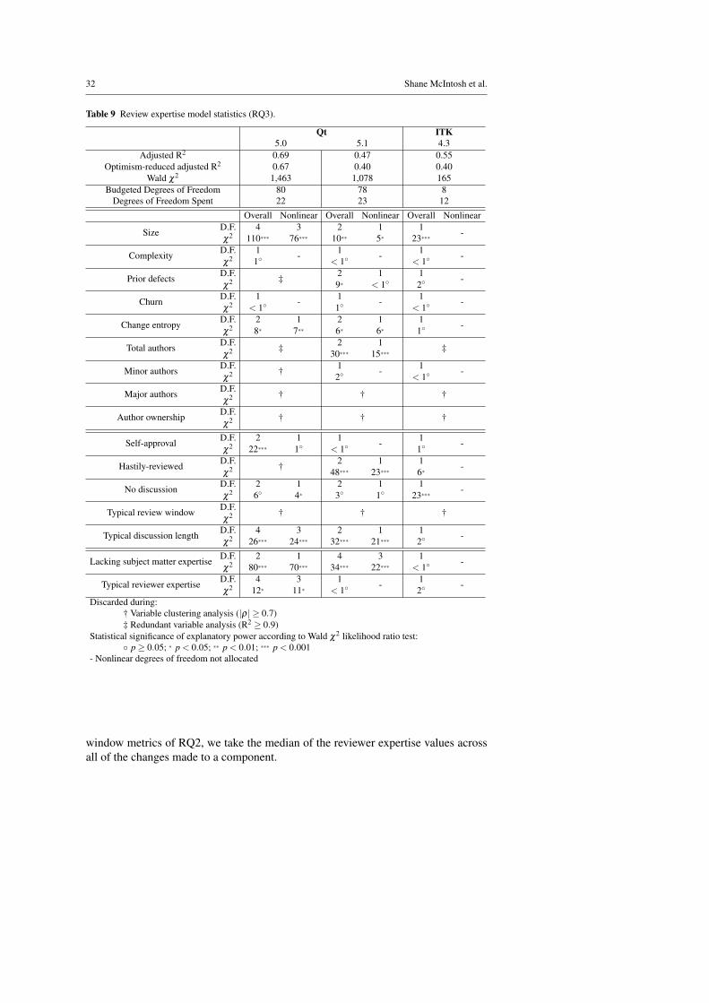
32 Shane McIntosh et al.
Table 9 Review expertise model statistics (RQ3).
Qt ITK5.0 5.1 4.3
Adjusted R2 0.69 0.47 0.55Optimism-reduced adjusted R2 0.67 0.40 0.40
Wald χ2 1,463 1,078 165Budgeted Degrees of Freedom 80 78 8
Degrees of Freedom Spent 22 23 12
Overall Nonlinear Overall Nonlinear Overall Nonlinear
Size D.F. 4 3 2 1 1 -χ2 110∗∗∗ 76∗∗∗ 10∗∗ 5∗ 23∗∗∗
Complexity D.F. 1 - 1 - 1 -χ2 1◦ < 1◦ < 1◦
Prior defects D.F. ‡ 2 1 1 -χ2 9∗ < 1◦ 2◦
Churn D.F. 1 - 1 - 1 -χ2 < 1◦ 1◦ < 1◦
Change entropy D.F. 2 1 2 1 1 -χ2 8∗ 7∗∗ 6∗ 6∗ 1◦
Total authors D.F. ‡ 2 1 ‡χ2 30∗∗∗ 15∗∗∗
Minor authors D.F. † 1 - 1 -χ2 2◦ < 1◦
Major authors D.F. † † †χ2
Author ownership D.F. † † †χ2
Self-approval D.F. 2 1 1 - 1 -χ2 22∗∗∗ 1◦ < 1◦ 1◦
Hastily-reviewed D.F. † 2 1 1 -χ2 48∗∗∗ 23∗∗∗ 6∗
No discussion D.F. 2 1 2 1 1 -χ2 6◦ 4∗ 3◦ 1◦ 23∗∗∗
Typical review window D.F. † † †χ2
Typical discussion length D.F. 4 3 2 1 1 -χ2 26∗∗∗ 24∗∗∗ 32∗∗∗ 21∗∗∗ 2◦
Lacking subject matter expertise D.F. 2 1 4 3 1 -χ2 80∗∗∗ 70∗∗∗ 34∗∗∗ 22∗∗∗ < 1◦
Typical reviewer expertise D.F. 4 3 1 - 1 -χ2 12∗ 11∗ < 1◦ 2◦
Discarded during:† Variable clustering analysis (|ρ| ≥ 0.7)‡ Redundant variable analysis (R2 ≥ 0.9)
Statistical significance of explanatory power according to Wald χ2 likelihood ratio test:◦ p≥ 0.05; ∗ p < 0.05; ∗∗ p < 0.01; ∗∗∗ p < 0.001
- Nonlinear degrees of freedom not allocated
window metrics of RQ2, we take the median of the reviewer expertise values acrossall of the changes made to a component.
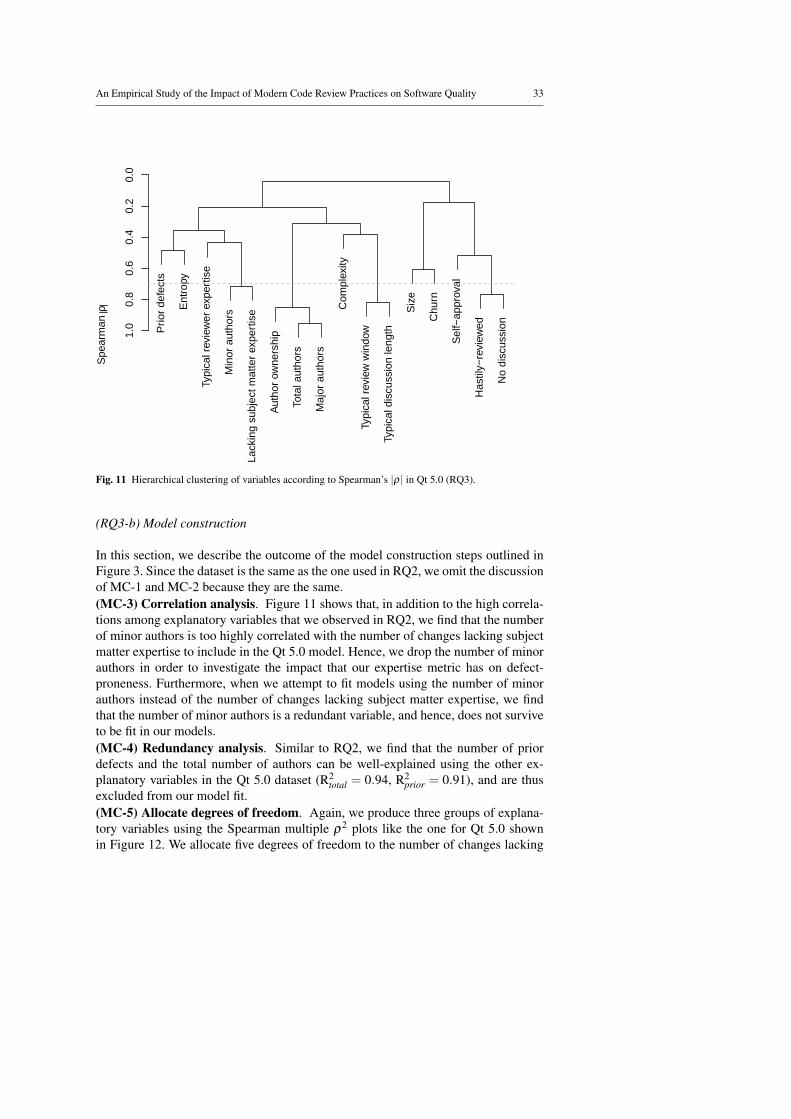
An Empirical Study of the Impact of Modern Code Review Practices on Software Quality 33
Prio
r de
fect
s
Ent
ropy
Typi
cal r
evie
wer
exp
ertis
e
Min
or a
utho
rs
Lack
ing
subj
ect m
atte
r ex
pert
ise
Aut
hor
owne
rshi
p
Tota
l aut
hors
Maj
or a
utho
rs
Com
plex
ity
Typi
cal r
evie
w w
indo
w
Typi
cal d
iscu
ssio
n le
ngth
Siz
e
Chu
rn
Sel
f−ap
prov
al
Has
tily−
revi
ewed
No
disc
ussi
on
1.0
0.8
0.6
0.4
0.2
0.0
Spe
arm
an ρ
Fig. 11 Hierarchical clustering of variables according to Spearman’s |ρ| in Qt 5.0 (RQ3).
(RQ3-b) Model construction
In this section, we describe the outcome of the model construction steps outlined inFigure 3. Since the dataset is the same as the one used in RQ2, we omit the discussionof MC-1 and MC-2 because they are the same.(MC-3) Correlation analysis. Figure 11 shows that, in addition to the high correla-tions among explanatory variables that we observed in RQ2, we find that the numberof minor authors is too highly correlated with the number of changes lacking subjectmatter expertise to include in the Qt 5.0 model. Hence, we drop the number of minorauthors in order to investigate the impact that our expertise metric has on defect-proneness. Furthermore, when we attempt to fit models using the number of minorauthors instead of the number of changes lacking subject matter expertise, we findthat the number of minor authors is a redundant variable, and hence, does not surviveto be fit in our models.(MC-4) Redundancy analysis. Similar to RQ2, we find that the number of priordefects and the total number of authors can be well-explained using the other ex-planatory variables in the Qt 5.0 dataset (R2
total = 0.94, R2prior = 0.91), and are thus
excluded from our model fit.(MC-5) Allocate degrees of freedom. Again, we produce three groups of explana-tory variables using the Spearman multiple ρ2 plots like the one for Qt 5.0 shownin Figure 12. We allocate five degrees of freedom to the number of changes lacking

34 Shane McIntosh et al.
Lacking subject matter expertiseSize
Self−approvalTypical discussion length
Typical reviewer expertiseChange entropy
No discussionComplexity
Churn
N df
1201 21201 21201 21201 21201 21201 21201 21201 21201 2●
●
●
●
●
●
●
●
●
0.05 0.15 0.25 0.35
Spearman ρ2 Response : Post − release defect count
Adjusted ρ2
Fig. 12 Dotplot of the Spearman multiple ρ2 of each explanatory variable and the post-release defectcount in Qt 5.0. Larger values indicate a more potential for non-monotonic relationship (RQ3).
subject matter expertise and component size. Three degrees of freedom are allocatedto the number of self-approved changes, typical discussion length, typical reviewerexpertise, change entropy, and the number of changes without discussion. Only onedegree of freedom is provided for component complexity and churn. We use a sim-ilar allocation process for the Qt 5.1 release. Due to the restrictive budget, we onlyallocate one degree of freedom for each explanatory variable in ITK.
(RQ3-c) Model Analysis
In this section, we describe the outcome of our model analysis outlined in Figure 3.(MA-1) Assessment of model stability. Table 9 shows that we achieve an adjustedR2 of between 0.47 (Qt 5.1) and 0.69 (Qt 5.0). While we find that our Qt models areonce again more stable than the ITK one, it is not surprising due to the difference insample sizes and that we needed to spend more degrees of freedom than our budgetsuggests. Nonetheless, the optimism-reduced adjusted R2 for ITK is 0.4, indicatingthat our ITK model still provides a reasonably robust fit.
Since these models were built using the same dataset as RQ2, they can be com-pared. We find that our expertise models of Table 9 do not outperform the partic-ipation models of Table 7 in terms of adjusted R2. In fact, the adjusted R2 of ourexpertise model in ITK is lower than that of its discussion model. This indicates thatthe expertise variables have not improved the unadjusted R2 by enough to offset thepenalty for adding additional explanatory variables.(MA-2) Estimate power of explanatory variables. Table 9 shows that our twoexpertise explanatory variables survive our model construction preprocessing to beincluded in the fit of all of our models. This suggests that expertise captures a dimen-sion of the datasets that is distinct. Moreover, Table 9 also shows that the number of

An Empirical Study of the Impact of Modern Code Review Practices on Software Quality 35
# changes lacking subject matter expertise
Pos
t−re
leas
e de
fect
cou
nt
0.0
0.5
1.0
1.5
2.0
0 20 40 60 80 100
(a) Lacking subject matter expertise (Qt 5.0)
# changes lacking subject matter expertise
Pos
t−re
leas
e de
fect
cou
nt
0.0
0.2
0.4
0 20 40 60
(b) Lacking subject matter expertise (Qt 5.1)
Fig. 13 The estimated count of post-release defects in a component for varying expertise metrics. Theblue line indicates the values of our model fit on the original data, while the grey area shows the 95%confidence interval based on models fit to 1,000 bootstrap samples.
changes lacking subject matter expertise has a significant impact on the defect modelsof both studied Qt releases. This suggests that subject matter expertise is an importantdimension to consider in defect models of large systems.
On the other hand, we find that neither expertise metric has a statistically sig-nificant impact on the ITK defect model. The difference in behaviour between Qtand ITK is likely due to the difference in team and system size. Table 1 shows thatthe Qt system is composed of 1,337-1,339 components, with code contributions from422-435 developers. Conversely, the ITK system only has 218 components, with con-tributions from 41 developers.
(MA-3) Examine explanatory variables in relation to the post-release defect count.Figure 13 shows that as the number of changes lacking subject matter expertise in-creases, so too does the estimated post-release defect count. Figure 13a shows anincreasing trend throughout the spectrum of observed numbers of changes lackingsubject matter expertise, albeit a slowing trend after a count of 8. Interestingly, Fig-ure 13b indicates that in Qt 5.1, there is a counter-intuitive drop in defect-pronenessas the number of changes lacking subject matter expertise increases from 0 to 1.Indeed, we find that 25 of the 200 components (13%), that have no changes lack-ing subject matter expertise, have at least one post-release defect, while 0 of the 87components with one change lacking subject matter expertise have any post-releasedefects. There are likely confounding factors that we have not controlled for thatwould explain why these components that do not lack subject matter expertise arestill defect-prone. Nonetheless, the drop in Figure 13b has only a small net impact of-0.09 on the estimated count of post-release defects.
Reviewer expertise has a measurable impact on post-release defect counts in thelarger studied releases. Components with many changes that lack subject matterexpertise tend to be defect-prone.
36 Shane McIntosh et al.
5 Threats to Validity
In this section, we discuss the threats to the validity of our case study.
5.1 External validity
We focus our study on three open source systems, due to the low number of sys-tems that satisfied our eligibility criteria for analysis. The proportion of commits thatunderwent code review through Gerrit presented a major challenge. Nonetheless, ad-ditional replication studies are needed.
5.2 Construct validity
Our models assume that each post-release defect is of the same weight, while inreality it may be that some post-release defects are more severe than others. Althoughmodern Issue Tracking Systems (ITS) provide a field for practitioners to denote thepriority and severity of a defect, recent work suggests that these fields are rarelyaccurate. For example, Herraiz et al. (2008) argue that the severity levels offered bythe Eclipse bug reporting tool do not agree with clusters of defects that form basedon the time taken to deliver a fix. Indeed, Mockus et al. (2002) find that the recordedpriority in Apache and Mozilla projects was not related to the time taken to resolvean issue, largely because the reporters who file the defects had far less experiencethan the core developers who fix them. Nonetheless, each defect that we consider asa quality-impacting post-release defect was at least severe enough to warrant a fix thatwas integrated into the strictly controlled release branches of the studied systems.
Furthermore, our models are incomplete, i.e., we have not measured all potentialdimensions that impact defect proneness. Other metrics that we may have overlookedmay better explain defect proneness than code review activity does. However, we feelthat our baseline metrics are strong, having been derived from the defect predictionliterature (Koru et al., 2009; Menzies et al., 2002; Graves et al., 2000; Nagappan andBall, 2005, 2007; Hassan, 2009; Bird et al., 2011).
5.3 Internal validity
We assume that a code review has been rushed if the elapsed time between the timethat a patch has been uploaded and the time that it has been approved is shorter thanthe amount of time that should have been spent if the reviewer was digesting 200lines of code per hour. However, there are likely cases where reviewers do not startreviewing the change immediately, but rush their review on a later date. Unfortu-nately, since reviewers do not record the time that they actually spent reviewing apatch, we must rely on heuristics to recover this information. On the other hand, ourheuristic is highly conservative, i.e., reviews that are flagged as rushed are certainlyrushed. Furthermore, setting the reviewing speed threshold to 100 lines per hour hadlittle impact on the observations derived from our models.
An Empirical Study of the Impact of Modern Code Review Practices on Software Quality 37
Since there is an inherent delay between the code review (and integration) ofa change and its appearance in a release, confounding factors could influence ourresults. However, our conclusions are intuitive, i.e., lax reviewing practices couldallow defects to permeate through to the release.
6 Discussion & Related Work
In this section, we discuss the broader implications of our findings and survey therelated work with respect to code review and software quality dimensions.
6.1 Discussion
Our results of Section 4 indicate that:
(RQ1) Since review coverage metrics are only significant contributors to two of thefour studied releases, there appears to be more to the relationship betweencode review practices and post-release defects than coverage alone can ex-plain.
(RQ2) Participation is a consistent contributor to our software quality models. Forall of the studied systems, metrics that capture the length of discussion andthe speed at which the review was performed offer statistically significantamounts of explanatory power to our models.
(RQ3) Expertise provides statistically significant explanatory power to our modelsof the large Qt system. However, participation metrics tend to have a largerimpact on our models than expertise metrics do.
Thus, we conclude that optimizing integration practices for coverage, i.e., enforc-ing a policy that ensures that a review has taken place for any new code change, maynot be sufficient to ensure that high quality code is shipped. Instead, software qual-ity concerns may be best addressed by monitoring code review participation whendeciding whether or not to integrate a code change into a codebase, making sure toinvolve subject matter experts.
Furthermore, our results relating to the relative impact of review participation andexpertise are echoed in the recent work of Rigby et al. (2014), who (like Porter et al.(1998)) build statistical models to study review efficiency, i.e., the amount of time thata review was open for discussion, and review effectiveness, i.e., the number of defectsdetected during a review. Rigby et al. find that an increase in review participationhas a larger impact on review effectiveness and efficiency than a similar increase inexperience or expertise does. This is in line with our results for defect proneness.
6.2 Code reviews
Prior work has qualitatively analyzed the modern code review process used by largesoftware systems. Rigby et al. (2008) find that the Apache project adopted a broadcast-based style of code review, where frequent reviews of small and independent changes

38 Shane McIntosh et al.
were in juxtaposition to the formal code inspection style prescribed by prior research,yet were still able to deliver a high level of software quality. In more recent work,Rigby and Storey (2011) find that open source developers that adopt the broadcast-based code review style actively avoid discussions in reviews about opinionated andtrivial patch characteristics. In our work, we find that active participation in the codereview process tends to reduce post-release counts and improve software quality.
The identification of defects is not the sole motivation for modern code review.For example, Rigby and Storey (2011) show that non-technical issues are a frequentmotivation for the patch rejection in several open source systems. Indeed, Baysalet al. (2013) find that review positivity, i.e., the proportion of accepted patches, isalso influenced by non-technical factors. Furthermore, a recent qualitative study atMicrosoft indicates that sharing knowledge among team members is also considereda very important motivation of modern code review (Bacchelli and Bird, 2013). In-spired by these studies, we empirically analyze the relationship between developerinvestment in the code review process and software quality.
Recent work has also shown that roughly 75% of the issues that are found (Mantylaand Lassenius, 2009) and fixed (Beller et al., 2014) during modern code reviews donot alter system behaviour. Rather than pointing out pertinent issues that may leadto defects, this large proportion of identified issues during code review aims to im-prove the maintainability of the code, with the intent of making future changes easier.Complementing their work, we find that components that are reviewed with activereviewer involvement tend to be less defect-prone, suggesting that these componentsare indeed more maintainable.
Kemerer and Paulk (2009) show that the introduction of design and code reviewto student projects at the SEI leads to code that is of higher quality. By studyingstudent projects, Kemerer and Paulk are able to control for several confounding fac-tors like team dynamics. Rather than control for team dynamics, our study aims tocomplement prior work by examining the impact of participation in the code reviewprocess of three large open source systems.
6.3 Software quality
There are many empirical studies that propose software metrics to predict softwarequality. For example, Hassan (2009) proposes complexity metrics (e.g., the changeentropy used in our paper) that are based on the code change process instead of onthe code. He shows that the entropy of the code change process is a good indicator ofdefect-prone source code files. Rahman and Devanbu (2013) built defect predictionmodels to compare the impact of product and process metrics. They show that productmetrics are generally less useful than process metrics for defect prediction. Througha case study of Eclipse, Kamei et al. (2010) also find that process metrics tend tooutperform product metrics when software quality assurance effort is considered. Inthis paper, our focus is on explaining the impact that modern code review practiceshave on software quality, rather than predicting it. Hence, we build models to studywhether metrics that measure code review coverage, participation, and expertise addunique information that helps to explain incidence rates of post-release defects.

An Empirical Study of the Impact of Modern Code Review Practices on Software Quality 39
Recent work studies the relationship between source code ownership and soft-ware quality. Bird et al. (2011) find that ownership measures have a strong relation-ship with both pre- and post-release defect-proneness. Matsumoto et al. (2010) showthat their proposed ownership measures (e.g., the number of developers and the codechurn generated by each developer) are also good indicators of defect-prone sourcecode files. Rahman and Devanbu (2011) find that lines of code that are changed toaddress a defect are more strongly associated with single developer contributions,suggesting that code review is a crucial part of software quality assurance. We findthat the code ownership metrics that we adopt in the baseline analysis of the studiedsystems are very powerful, contributing a statistically significant amount of explana-tory power to each of the defect models that we built.
7 Conclusions
Although code reviewing is a broadly endorsed best practice for software develop-ment, little work has empirically evaluated the impact that properties of the moderncode review process have on software quality in large software systems. With the re-cent emergence of modern code reviewing tools like Gerrit, high quality data is nowbecoming available to enable such empirical studies.
The lightweight nature of modern code review processes relaxes the strict criteriaof the formal code inspections that were mandated to ensure that a basic level ofreview participation was achieved (e.g., in-person meetings and reviewer checklists).In this paper, we quantitatively investigate three large software systems using moderncode review tools (i.e., Gerrit). We build and analyze regression models that explainthe incidence of post-release defects in the components of these systems. Specifically,we evaluate the conjecture that:
If a large proportion of the code changes that are integrated duringdevelopment are either: (1) omitted from the code review process(low review coverage), (2) have lax code review involvement (lowreview participation), or (3) do not include a subject matter expert(low expertise), then defect-prone code will permeate through to thereleased software product.
The results of our case study indicate that:
– Code review coverage metrics only contribute a significant amount of explanatorypower to two of the four defect models when we control for several metrics thatare known to be good explainers of software quality. This suggests that whilecode review coverage is an important quality to attain, other properties of thecode reviewing process are likely at play.
– Discussion-related code review participation metrics contribute significant amountsof explanatory power to the defect models of each of the studied releases. Met-rics related to review participation should be considered when making integrationdecisions.

40 Shane McIntosh et al.
– Expertise-related metrics that include data from the code review process also pro-vide significant amounts of explanatory power to defect models of the larger Qtreleases. Teams should aim to ensure that if a subject matter expert is not availableto fix a component, they should be involved in the code reviewing process.
We believe that our findings provide strong empirical evidence to support thedesign of modern code integration policies that take code review coverage, participa-tion, and expertise into consideration. Our models suggest that such policies will leadto higher quality, less defect-prone software.
8 Acknowledgments
The authors would like to acknowledge Frank Harrell Jr. for the insightful discus-sions and assistance with the configuration and debugging of the rms R package. Theauthors would also like to thank Peter C. Rigby and the anonymous reviewers fortheir fruitful comments on earlier versions of this work.
This research was partially supported by the Natural Sciences and Engineer-ing Research Council of Canada (NSERC) and JSPS KAKENHI Grant Numbers24680003 and 25540026.
References
Bacchelli A, Bird C (2013) Expectations, Outcomes, and Challenges of Modern CodeReview. In: Proc. of the 35th Int’l Conf. on Software Engineering (ICSE), pp 712–721
Baysal O, Kononenko O, Holmes R, Godfrey MW (2013) The Influence of Non-technical Factors on Code Review. In: Proc. of the 20th Working Conf. on ReverseEngineering (WCRE), pp 122–131
Beller M, Bacchelli A, Zaidman A, Juergens E (2014) Modern Code Reviews inOpen-Source Projects: Which Problems Do They Fix? In: Proc. of the 11th Work-ing Conf. on Mining Software Repositories (MSR), pp 202–211
Bettenburg N, Hassan AE, Adams B, German DM (2014) Management of commu-nity contributions: A case study on the Android and Linux software ecosystems.Empirical Software Engineering To appear
Bird C, Nagappan N, Murphy B, Gall H, Devanbu P (2011) Don’t Touch My Code!Examining the Effects of Ownership on Software Quality. In: Proc. of the 8th jointmeeting of the European Software Engineering Conf. and the Symposium on theFoundations of Software Engineering (ESEC/FSE), pp 4–14
Chambers JM, Hastie TJ (eds) (1992) Statistical Models in S, Wadsworth and Brook-s/Cole, chap 4
Efron B (1986) How Biased is the Apparent Error Rate of a Prediction Rule? Journalof the American Statistical Association 81(394):461–470
Fagan ME (1976) Design and Code Inspections to Reduce Errors in Program Devel-opment. IBM Systems Journal 15(3):182–211

An Empirical Study of the Impact of Modern Code Review Practices on Software Quality 41
Graves TL, Karr AF, Marron JS, Siy H (2000) Predicting Fault Incidence using Soft-ware Change History. Transactions on Software Engineering (TSE) 26(7):653–661
Hamasaki K, Kula RG, Yoshida N, Cruz AEC, Fujiwara K, Iida H (2013) Who DoesWhat during a Code Review? Datasets of OSS Peer Review Repositories. In: Proc.of the 10th Working Conf. on Mining Software Repositories (MSR), pp 49–52
Harrell Jr FE (2002) Regression Modeling Strategies, 1st edn. SpringerHarrell Jr FE (2014) rms: Regression Modeling Strategies. URL http://biostat.
mc.vanderbilt.edu/rms, r package version 4.2-1Harrell Jr FE, Lee KL, Califf RM, Pryor DB, Rosati RA (1984) Regression modelling
strategies for improved prognostic prediction. Statistics in Medicine 3(2):143–152Harrell Jr FE, Lee KL, Matchar DB, Reichert TA (1985) Regression models for prog-
nostic prediction: advantages, problems, and suggested solutions. Cancer Treat-ment Reports 69(10):1071–1077
Hassan AE (2008) Automated Classification of Change Messages in Open SourceProjects. In: Proc. of the 23rd Int’l Symposium on Applied Computing (SAC), pp837–841
Hassan AE (2009) Predicting Faults Using the Complexity of Code Changes. In:Proc. of the 31st Int’l Conf. on Software Engineering (ICSE), pp 78–88
Hastie T, Tibshirani R, Friedman J (2009) Elements of Statistical Learning, 2nd edn.Springer
Herraiz I, German DM, Gonzalez-Barahona JM, Robles G (2008) Towards a Simpli-fication of the Bug Report form in Eclipse. In: Proc. of the 5th Working Conf. onMining Software Repositories (MSR), pp 145–148
Jiang Y, Adams B, German DM (2013) Will My Patch Make It? And How Fast?:Case Study on the Linux Kernel. In: Proc. of the 10th Working Conf. on MiningSoftware Repositories (MSR), pp 101–110
Kamei Y, Matsumoto S, Monden A, ichi Matsumoto K, Adams B, Hassan AE (2010)Revisiting Common Bug Prediction Findings Using Effort-Aware Models. In:Proc. of the 26th Int’l Conf. on Software Maintenance (ICSM), pp 1–10
Kamei Y, Shihab E, Adams B, Hassan AE, Mockus A, Sinha A, Ubayashi N (2013)A Large-Scale Empirical Study of Just-in-Time Quality Assurance. Transactionson Software Engineering (TSE) 39(6):757–773
Kemerer CF, Paulk MC (2009) The Impact of Design and Code Reviews on Soft-ware Quality: An Empirical Study Based on PSP Data. Transactions on SoftwareEngineering (TSE) 35(4):534–550
Kim S, Whitehead EJ Jr, Zhang Y (2008) Classifying software changes: Clean orbuggy? Transactions on Software Engineering (TSE) 34(2):181–196
Koru AG, Zhang D, Emam KE, Liu H (2009) An Investigation into the FunctionalForm of the Size-Defect Relationship for Software Modules. Transactions on Soft-ware Engineering (TSE) 35(2):293–304
Mantyla MV, Lassenius C (2009) What Types of Defects Are Really Discovered inCode Reviews? Transactions on Software Engineering (TSE) 35(3):430–448
Matsumoto S, Kamei Y, Monden A, ichi Matsumoto K, Nakamura M (2010) Ananalysis of developer metrics for fault prediction. In: Proc. of the 6th Int’l Conf.on Predictive Models in Software Engineering (PROMISE), pp 18:1–18:9

42 Shane McIntosh et al.
McCabe TJ (1976) A complexity measure. In: Proc. of the 2nd Int’l Conf. on Soft-ware Engineering (ICSE), p 407
McIntosh S, Kamei Y, Adams B, Hassan AE (2014) The Impact of Code ReviewCoverage and Code Review Participation on Software Quality: A Case Study ofthe QT, VTK, and ITK Projects. In: Proc. of the 11th Working Conf. on MiningSoftware Repositories (MSR), pp 192–201
Menzies T, Stefano JSD, Chapman M, McGill K (2002) Metrics That Matter. In:Proc of the 27th Annual NASA Goddard/IEEE Software Engineering Workshop,pp 51–57
Mockus A, Votta LG (2000) Identifying Reasons for Software Changes Using His-toric Databases. In: Proc. of the 16th Int’l Conf. on Software Maintenance (ICSM),pp 120–130
Mockus A, Weiss DM (2000) Predicting Risk of Software Changes. Bell Labs Tech-nical Journal 5(2):169–180
Mockus A, Fielding RT, Herbsleb JD (2002) Two Case Studies of Open Source Soft-ware Development: Apache and Mozilla. Transactions On Software Engineeringand Methodology (TOSEM) 11(3):309–346
Mukadam M, Bird C, Rigby PC (2013) Gerrit Software Code Review Data fromAndroid. In: Proc. of the 10th Working Conf. on Mining Software Repositories(MSR), pp 45–48
Nagappan N, Ball T (2005) Use of relative code churn measures to predict systemdefect density. In: Proc. of the 27th Int’l Conf. on Software Engineering (ICSE),pp 284–292
Nagappan N, Ball T (2007) Using Software Dependencies and Churn Metrics to Pre-dict Field Failures: An Empirical Case Study. In: Proc. of the 1st Int’l Symposiumon Empirical Software Engineering and Measurement (ESEM), pp 364–373
Nagappan N, Ball T, Zeller A (2006) Mining metrics to predict component failures.In: Proc. of the 28th Int’l Conf. on Software Engineering (ICSE), pp 452–461
Porter A, Siy H, Mockus A, Votta L (1998) Understanding the Sources of Variationin Software Inspections. Transactions On Software Engineering and Methodology(TOSEM) 7(1):41–79
R Core Team (2013) R: A Language and Environment for Statistical Computing.R Foundation for Statistical Computing, Vienna, Austria, URL http://www.
R-project.org/
Rahman F, Devanbu P (2011) Ownership, Experience and Defects: A Fine-GrainedStudy of Authorship. In: Proc. of the 33rd Int’l Conf. on Software Engineering(ICSE), pp 491–500
Rahman F, Devanbu P (2013) How, and why, process metrics are better. In: Proc. ofthe 35th Int’l Conf. on Software Engineering (ICSE), pp 432–441
Rigby PC, Bird C (2013) Convergent Contemporary Software Peer Review Practices.In: Proc. of the 9th joint meeting of the European Software Engineering Conf. andthe Symposium on the Foundations of Software Engineering (ESEC/FSE), pp 202–212
Rigby PC, Storey MA (2011) Understanding Broadcast Based Peer Review on OpenSource Software Projects. In: Proc. of the 33rd Int’l Conf. on Software Engineering(ICSE), pp 541–550

An Empirical Study of the Impact of Modern Code Review Practices on Software Quality 43
Rigby PC, German DM, Storey MA (2008) Open Source Software Peer Review Prac-tices: A Case Study of the Apache Server. In: Proc. of the 30th Int’l Conf. onSoftware Engineering (ICSE), pp 541–550
Rigby PC, German DM, Cohen L, Storey MA (2014) Peer Review on Open SourceSoftware Projects: Parameters, Statistical Models, and Theory. Transactions OnSoftware Engineering and Methodology (TOSEM) To appear
Sarle WS (1990) The VARCLUS Procedure. In: SAS/STAT User’s Guide, 4th edn,SAS Institute, Inc.
Shannon CE (1948) A Mathematical Theory of Communication. The Bell SystemTechnical Journal 27:379–423, 623–656
Shihab E, Mockus A, Kamei Y, Adams B, Hassan AE (2011) High-Impact Defects:A Study of Breakage and Surprise Defects. In: Proc. of the 8th joint meeting of theEuropean Software Engineering Conf. and the Symposium on the Foundations ofSoftware Engineering (ESEC/FSE), pp 300–310
Tanaka T, Sakamoto K, Kusumoto S, ichi Matsumoto K, Kikuno T (1995) Improve-ment of Software Process by Process Description and Benefit Estimation. In: Proc.of the 17th Int’l Conf. on Software Engineering (ICSE), pp 123–132
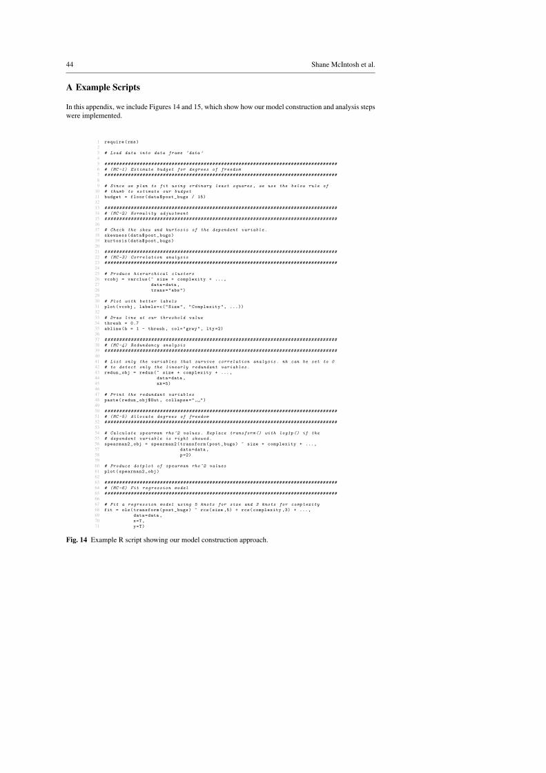
44 Shane McIntosh et al.
A Example Scripts
In this appendix, we include Figures 14 and 15, which show how our model construction and analysis stepswere implemented.
1 require(rms)
23 # Load data into data frame ‘data ’
45 # ###############################################################################
6 # (MC -1) Estimate budget for degrees of freedom
7 # ###############################################################################
89 # Since we plan to fit using ordinary least squares , we use the below rule of
10 # thumb to estimate our budget
11 budget = floor(data$post_bugs / 15)
1213 # ###############################################################################
14 # (MC -2) Normality adjustment
15 # ###############################################################################
1617 # Check the skew and kurtosis of the dependent variable.
18 skewness(data$post_bugs)
19 kurtosis(data$post_bugs)
2021 # ###############################################################################
22 # (MC -3) Correlation analysis
23 # ###############################################################################
2425 # Produce hierarchical clusters
26 vcobj = varclus(~ size + complexity + ...,
27 data=data ,
28 trans="abs")
2930 # Plot with better labels
31 plot(vcobj , labels=c("Size", "Complexity", ...))
3233 # Draw line at our threshold value
34 thresh = 0.7
35 abline(h = 1 - thresh , col="grey", lty =2)
3637 # ###############################################################################
38 # (MC -4) Redundancy analysis
39 # ###############################################################################
4041 # List only the variables that survive correlation analysis. nk can be set to 0
42 # to detect only the linearly redundant variables.
43 redun_obj = redun(~ size + complexity + ...,
44 data=data ,
45 nk=5)
4647 # Print the redundant variables
48 paste(redun_obj$Out , collapse=", ")
4950 # ###############################################################################
51 # (MC -5) Allocate degrees of freedom
52 # ###############################################################################
5354 # Calculate spearman rho ^2 values. Replace transform () with log1p () if the
55 # dependent variable is right skewed.
56 spearman2_obj = spearman2(transform(post_bugs) ~ size + complexity + ...,
57 data=data ,
58 p=2)
5960 # Produce dotplot of spearman rho ^2 values
61 plot(spearman2_obj)
6263 # ###############################################################################
64 # (MC -6) Fit regression model
65 # ###############################################################################
6667 # Fit a regression model using 5 knots for size and 3 knots for complexity
68 fit = ols(transform(post_bugs) ~ rcs(size ,5) + rcs(complexity ,3) + ...,
69 data=data ,
70 x=T,
71 y=T)
Fig. 14 Example R script showing our model construction approach.

An Empirical Study of the Impact of Modern Code Review Practices on Software Quality 45
1 require(rms)
23 # Load data into data frame ‘data ’
45 # Load model fit into ‘fit ’
67 # ###############################################################################
8 # (MA -1) Assessment of model stability
9 # ###############################################################################
1011 # Run the bootstrapped optimism calculations
12 num_iter = 1000
13 validate(fit , B=num_iter)
1415 # ###############################################################################
16 # (MA -2) Estimate power of explanatory variables
17 # ###############################################################################
1819 # Print the Wald chi ^2 likelihood ratio test results
20 anova(fit , test="Chisq")
2122 # ###############################################################################
23 # (MA -3) Examine variables in relation to outcome
24 # ###############################################################################
2526 # Store bootstrap results in an object
27 bootcov_obj = bootcov(fit , B=num_iter)
2829 # Plot the response curve for the ‘size ’ variable. If the dependent variable
30 # was transformed , undo the transformation here using the ‘fun ’ parameter .
31 response_curve = Predict(bootcov_obj ,
32 size ,
33 fun=function(x) return(undo_transform(x)))
34 plot(response_curve)
Fig. 15 Example R script showing our model analysis approach.


![Software Reviews - Hasso Plattner Institute · Code Reviews —Software Engineering II Review Definition “[Formal or informal] meeting during which a software product is [examined](https://static.fdocuments.us/doc/165x107/5f0711c37e708231d41b2640/software-reviews-hasso-plattner-institute-code-reviews-asoftware-engineering.jpg)