An empirical analysis of disability and household ...
44
An empirical analysis of disability and household expenditure allocations Hong il Yoo School of Economics University of New South Wales
Transcript of An empirical analysis of disability and household ...

An empirical analysis of disability and household
expenditure allocations
Hong il Yoo
School of Economics
University of New South Wales

Introduction
Disability may influence household expenditure allocations in
several dimensions
– Eg loss of earnings potential, constraints on time inputs
This study is based on an Engel curve analysis
– Focus on current expenditure allocation across non-durable goods
– Model to be estimated is static & covers market goods
– Empirical applications have been rare
Jones and O‟Donnell (J. Pub Econ, ‟95) :
– Compares Engel curves of childless couples w/ disability vs
couples w/o disability in a unitary setting

Introduction
Extend Jones & O‟Donnell‟s analysis with benefit from recent
advance in demand analysis
– A collective model due to Lewbel & Pendakur (‟08)
In a childless couple household, how does disability of one
spouse affect :
– Intra-household resource allocation between spouses &
– the extent to which goods are jointly consumed,
– after taking into account individual-level preference changes due
to disability?
Very little is known about these issues

Overview
Primary data source:
– Canadian Survey of Household Spending ‟04-‟07
Major findings
– Individual Engel curve estimates show expected responses to
disability eg. spend less on clothing, more on hhld ops.
– Sharing rule is more precisely estimated than economies of scale
• Variations in total expenditures help identify both
• But sharing rule has other sources of variations too
– Own disability reduces woman‟s share of resources by 3~6 % pts
while spousal disability increases it by 4~9% pts.
– Some estimates suggest that disability reduces benefits from joint
consumption but too imprecise to warrant firm conclusions

Literature
Recent interest in the impact of disability on household
consumption from the policy literature
– Tibble (‟05) and Stapleton et al. (‟08) for extensive reviews
Objective is to analyse extra costs of living associated with
disability instead of earnings losses
– Intended to inform disability allowance programs
“The standard of living approach” is gaining popularity
– Similar concept as equivalence scales in microeconomic demand
analysis

Literature
Disability recognised as an area of application in theoretical
contributions eg Lewbel (‟85) and Blackorby & Donaldson („92)
Empirical applications have been rare
– Most household expenditure surveys collect no info on disability
The only exception?: Jones and O‟Donnell (J.Pub Eco, ‟95)
– Uses a one-off supplement to UK Family Expenditure Survey
– Focuses on equivalence scales which can be estimated from a
single equation regression over a single cross section
– Compares Engel curves of childless couples w/o disability vs
childless couples w/ disability

Literature
Jones & O‟Donnell (‟95) – ctd.
– Under certain restrictions on preferences, conclude that a disabled
couple needs to spend at least 40~70% more to be as well off as
a non-disabled couple
– A possible interpretation: disability affects the extent to which
goods can be jointly consumed within the household
The present analysis extends Jones & O‟Donnell‟s analysis by
incorporating recent advance in demand analysis
– Estimate a collective Engel curve system previously applied to
‟90-‟92 Canadian data (Lewbel & Pendakur, ‟08) and ‟05 Irish data
(Bargain et al., ‟10) (These papers did not incorporate health or
disability in the analysis)
Motivation
Consider person A who may marry a disabled person B or a non-
disabled person C
What may explain differences in spending patterns of couple
{A, B} and couple {A,C} ?
One simple answer: B‟s preferences are different from C‟s
Another: structural components of interest
– Disability may affect jointness of consumption goods
– and how household resources are shared between spouses
Motivation
Can we disentangle preference differences from the structural
components at least to some extent?
Evidence on the economies of scale changes over and above
preference changes may provide a strong economic justification
for policy intervention
Information on changes in resource shares may be relevant for
poverty & inequality analysis

Modelling framework
A collective household demand model of Browning, Chiappori &
Lewbel (unpublished; ‟09)
Key features :
– Intrahousehold resource allocation is Pareto efficient
– Total consumption of husband & wife > expenditure on goods
• Due to jointness of consumption
• Incorporated into the model using “Barten-Gorman” technology
– Assume that preferences remain stable before & after marriage
• ie relevant preference changes can be parametrised independently
– Combine data on singles and couples to recover sharing rule &
economies of scale

Empirical specification
Given the short span of data, estimate a collective Engel curve
system instead of a demand system with price variations
– Lewbel and Pendakur (J.Econometrics; ‟08) develops relevant
restrictions on preferences
– Structural in the sense that the sharing rule and the economies of
scale parameters are separately identified
Model specification consists of three building blocks summarised
below

Empirical specification
Step 1: Specify individual Engel curves incorporating preference
changes due to disability (& other demographic controls)
– These are estimated from data on singles (and couples)
Step 2: Construct household Engel curves by combining
individual Engel curves according to the theoretical structure
– Economies of scale and sharing rule functions are introduced into
the system
Step 3: Parameterise economies of scale & sharing rule
– The new parameters are estimated from data on couples

Step 1: Specifying individual Engel curves
First, specify an individual Engel curve system which
incorporates preference differences b/w person B and C
A parsimonious specification:
– Introduce demographics including disability into a quadratic Engel
curve system using Shape Invariance transformation
– k = 1,2,…,K goods - i = male, female
– zi = vector of demographic characteristics including disability
– ln y = log of expenditure budget
0 2' (ln ' ) (ln ' )
( , )
k k k k k k
i i i i i i i i i i i
k k
i i i
w a a z b y e z c y e z
w y z
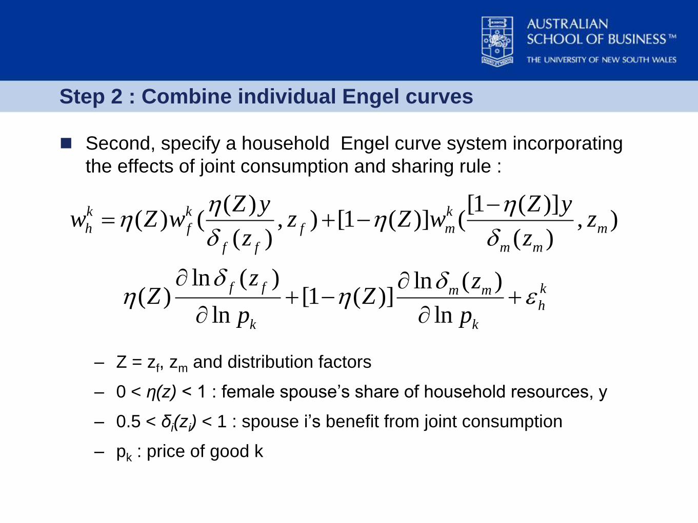
Step 2 : Combine individual Engel curves
Second, specify a household Engel curve system incorporating
the effects of joint consumption and sharing rule :
– Z = zf, zm and distribution factors
– 0 < η(z) < 1 : female spouse‟s share of household resources, y
– 0.5 < δi(zi) < 1 : spouse i‟s benefit from joint consumption
– pk : price of good k
( ) [1 ( )]( ) ( , ) [1 ( )] ( , )
( ) ( )
ln ( ) ln ( )( ) [1 ( )]
ln ln
k k k
h f f m m
f f m m
f f km mh
k k
Z y Z yw Z w z Z w z
z z
z zZ Z
p p
Step 3: Parameterise economies of scale & sharing rule
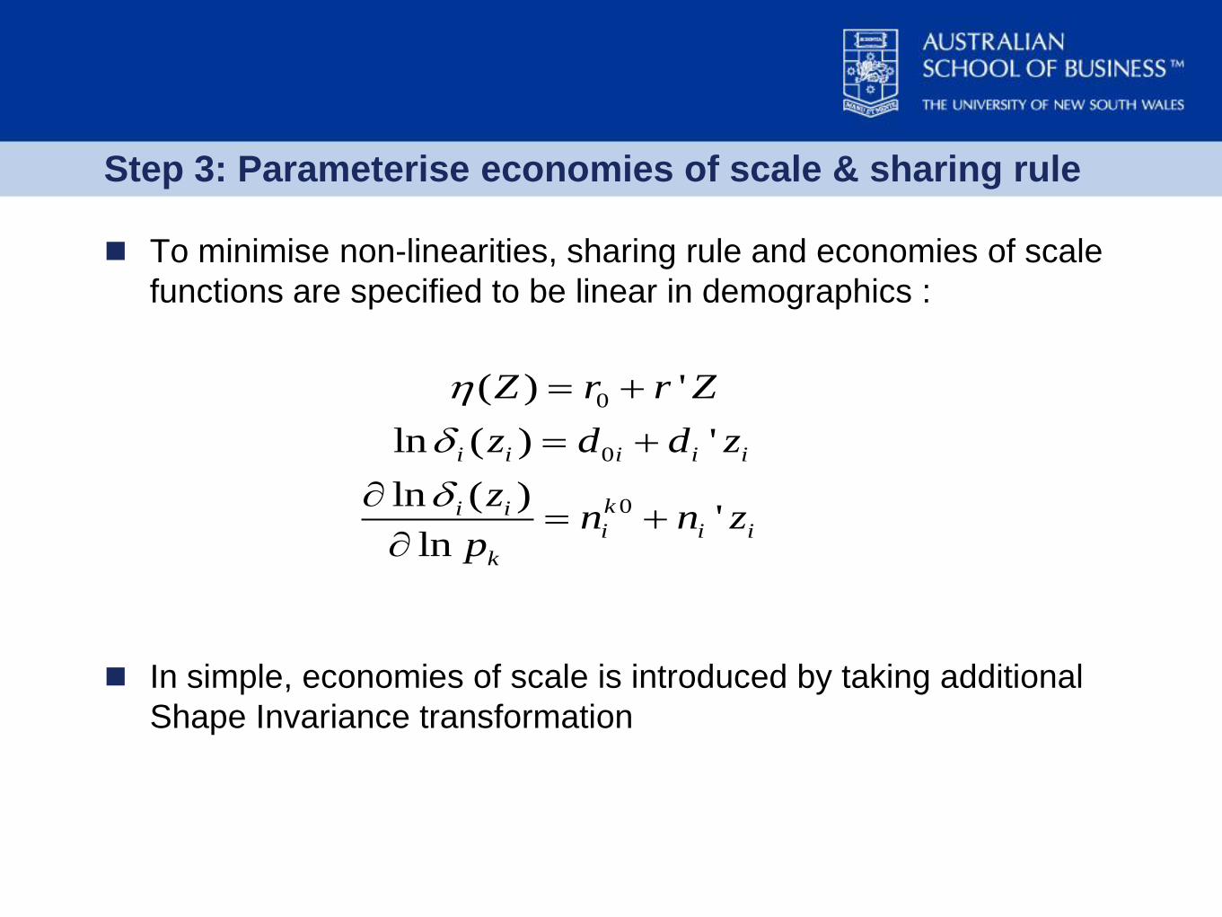
To minimise non-linearities, sharing rule and economies of scale
functions are specified to be linear in demographics :
In simple, economies of scale is introduced by taking additional
Shape Invariance transformation
0
0
0
( ) '
ln ( ) '
ln ( )'
ln
i i i i i
ki ii i i
k
Z r r Z
z d d z
zn n z
p
Empirical specification : An example
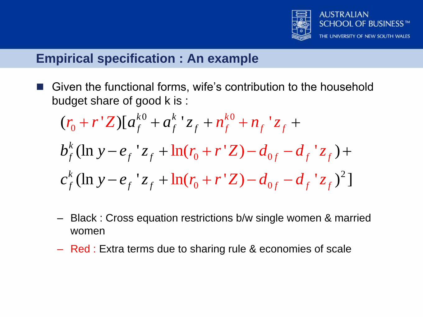
Given the functional forms, wife‟s contribution to the household
budget share of good k is :
– Black : Cross equation restrictions b/w single women & married
women
– Red : Extra terms due to sharing rule & economies of scale
0
2
0
0
0 0
0 0
( )[ '
(ln ' )
(ln ' )
' '
ln( ' ) '
ln( ' ) ]'
k k
f f f
k
f
k
f
f f
k
f f
f f
f f f
f f ff
r r Z n n z
r r
a a z
Z d d z
r r Z d
b y e
d
z
c y e z z

Empirical specification
The key identifying assumption of this model is that single and
married individuals share the same Engel curve parameters in
Thus joint estimation of singles‟ and couples‟ Engel curve
systems allows recovery of the structural components
– Below, estimation is done by FGNLS on TSP 5.1
Fairly restrictive if singles‟ preferences are fundamentally
different from those who choose to marry
– For robustness checks, restrict the sample of singles to those who
have been previously married
( , ) & ( , )k k
m m f fw y z w y z

Empirical specification
To sum up, the Engel curve system looks like:
( , )
( , )
( ) [1 ( )]( ) ( , ) [1 ( )] ( , ) ( )
( ) ( )
k k k
f f f f
k k k
m m m m
k k k k k
h f f m m h h
f f m m
w w y z
w w y z
y y y yw Z w z Z w z n Z
z z
( , , , )
, , '
i i i i
f m
z age educ work
Z z z woman s shareof household income
idisability

Data : an overview
Canadian Survey of Household Spending, ‟04-‟07
– Cross sectional recall data on household spending
– Provides an individual-level disability indicator for the reference
person and his/her spouse
– Defined as presence of physical, mental or health conditions
which induce activity limitations
– Severity index is not provided
• Key limitation of these data
• In Jones and O‟Donnell‟s (‟95) UK study, severity or type of condition
not found to be significant
• Some informal sensitivity checks have been done using percentiles of
total OOP health expenditure

Data : sampling choices
Basic sampling criteria follow Lewbel and Pendakur (‟08) :
– To facilitate comparison with the previous study
– Childless singles and couples
– reside in large urban areas (minimise effects on home production)
– aged 26-59 (minimise labour market entry & exit effects)
– Live on rented dwellings (rent not observed for home owners)
Choice of pooling cross sections time periods
– Engel curve analysis assumes constant prices
– Pooling cross sections increase sample size
• Particularly important as a small fraction of the sample is disabled
– This presentation focuses on ‟04-‟05 and ‟04-‟07 results

Data : sampling choices
Total expenditure budget has been deflated by CPI from
Statistics Canada
– An alternative may be to construct a Stone index or use provincial
deflators
– Inflation rate between ‟04 and ‟07 has been 6% nationwide
• 2% b/w ‟04 and ‟05
– Relative price changes yet to be checked
Data : expenditure classification
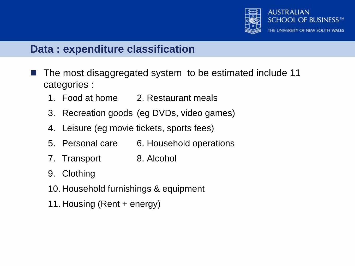
The most disaggregated system to be estimated include 11
categories :
1. Food at home 2. Restaurant meals
3. Recreation goods (eg DVDs, video games)
4. Leisure (eg movie tickets, sports fees)
5. Personal care 6. Household operations
7. Transport 8. Alcohol
9. Clothing
10. Household furnishings & equipment
11. Housing (Rent + energy)

Data – key features
‟04-‟05 data
– 2,051 households in total : 1,522 singles + 529 couples
– 667 single women in total : 135 disabled (21%)
– 845 single men in total : 163 disabled (19%)
– 529 couples in total: 63 disabled men (12%) & 59 women (11%)
‟04-‟07 data
– 3,971 households in total : 2,966 singles + 1,008 couples
– 1,308 single women in total : 292 disabled (22%)
– 1,658 single men in total : 313 disabled (19%)
– 1,008 couples in total : 116 disabled men (12%) & 115 women
(11%)

Data – key features
It is likely that disabled singles face less severe restrictions than
their counterparts in couples on average
– Given the model specification, the impact on the economies of
scale may be contaminated by the impact of severity increase
Raw data on budget shares show that spending pattern
differences exist between disabled & non-disabled singles
though
– Eg budget share of food at home (restaurant meals) is 0.02 higher
(lower) for disabled singles
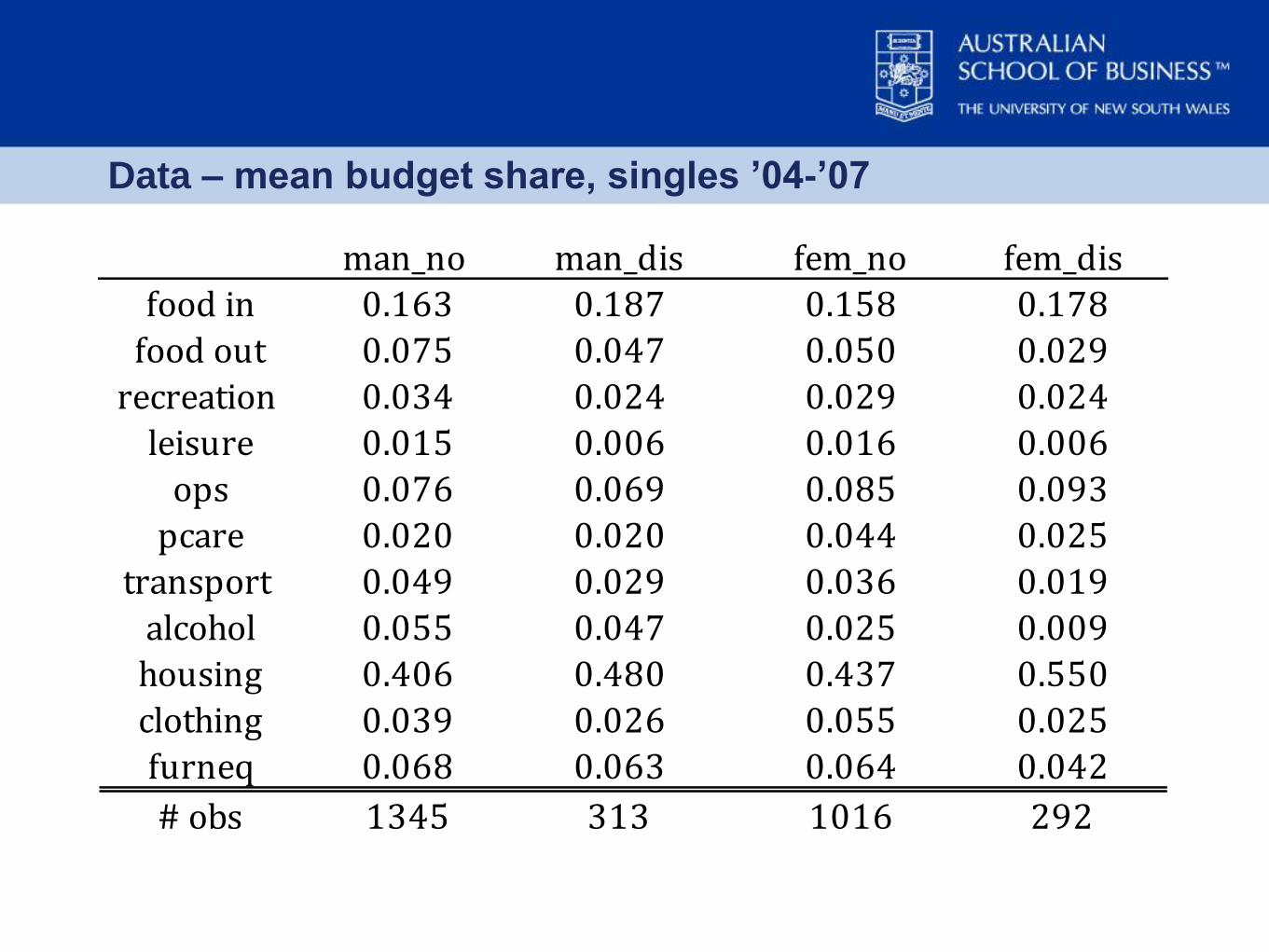
Data – mean budget share, singles ’04-’07
man_no man_dis fem_no fem_dis
food in 0.163 0.187 0.158 0.178
food out 0.075 0.047 0.050 0.029
recreation 0.034 0.024 0.029 0.024
leisure 0.015 0.006 0.016 0.006
ops 0.076 0.069 0.085 0.093
pcare 0.020 0.020 0.044 0.025
transport 0.049 0.029 0.036 0.019
alcohol 0.055 0.047 0.025 0.009
housing 0.406 0.480 0.437 0.550
clothing 0.039 0.026 0.055 0.025
furneq 0.068 0.063 0.064 0.042
# obs 1345 313 1016 292

Data – mean budget shares, couples ’04-’07
no_dis man_dis fem_dis both_dis
food in 0.181 0.185 0.215 0.208
food out 0.059 0.046 0.036 0.033
recreation 0.033 0.029 0.026 0.037
leisure 0.017 0.008 0.004 0.004
ops 0.079 0.093 0.108 0.077
pcare 0.036 0.034 0.030 0.022
transport 0.062 0.048 0.050 0.049
alcohol 0.033 0.036 0.035 0.034
housing 0.354 0.416 0.387 0.418
clothing 0.070 0.043 0.038 0.039
furneq 0.076 0.061 0.070 0.079
# obs 826 67 66 49

Estimation strategy
1. Choose the level of disaggregation
– Here I summarise the results from 11, 9 and 7 category systems
– To reduce the number of parameters to be estimated
– Check for robustness to expenditure classifications
2. Start with a full set of demographic characteristics (age,
college education, employment & disability). Drop the
employment dummy. Drop the education dummy.
3. Check for parametric restrictions which may improve
statistical precision of economies of scale estimates
– Eg restricting slope coefficients across genders
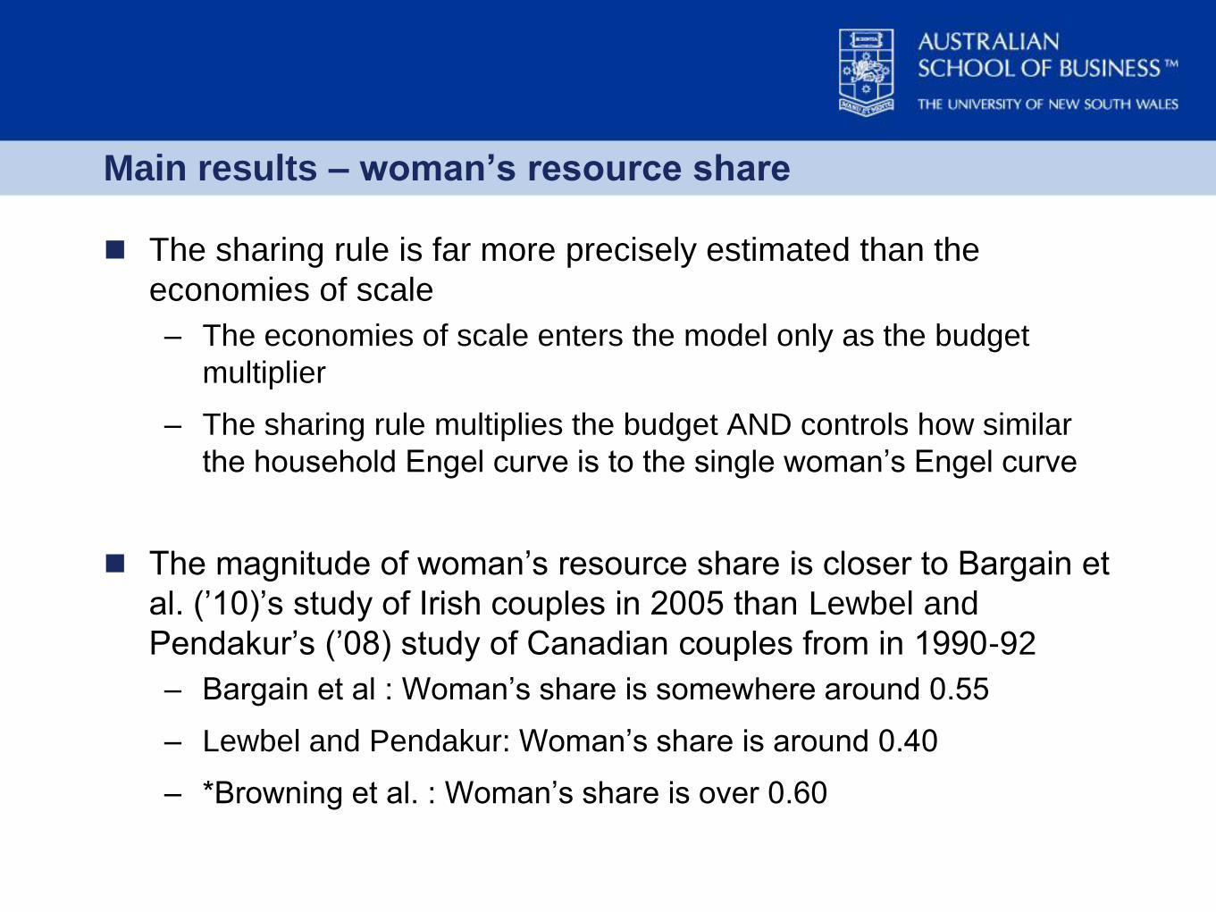
Main results – woman’s resource share
The sharing rule is far more precisely estimated than the
economies of scale
– The economies of scale enters the model only as the budget
multiplier
– The sharing rule multiplies the budget AND controls how similar
the household Engel curve is to the single woman‟s Engel curve
The magnitude of woman‟s resource share is closer to Bargain et
al. (‟10)‟s study of Irish couples in 2005 than Lewbel and
Pendakur‟s (‟08) study of Canadian couples from in 1990-92
– Bargain et al : Woman‟s share is somewhere around 0.55
– Lewbel and Pendakur: Woman‟s share is around 0.40
– *Browning et al. : Woman‟s share is over 0.60

Main results – woman’s resource share
The reference couple :
-Both spouses aged 40 -Both without college education
-Both without disability -(Both outside full-time employment)
-Wife contributes 40% of the couple‟s pre-tax income
In ‟04-‟05 sample, the reference wife‟s resource share estimate is
a bit above 0.50 in general with t ratios well in excess of 4
– Some variations depending on demographic controls
– 0.52 in 11-goods, 0.50~0.53 in 9-goods and 0.50~0.56 in 7-goods
– Similar to ‟04-‟07 sample, though there the resource share is a bit
below 0.50
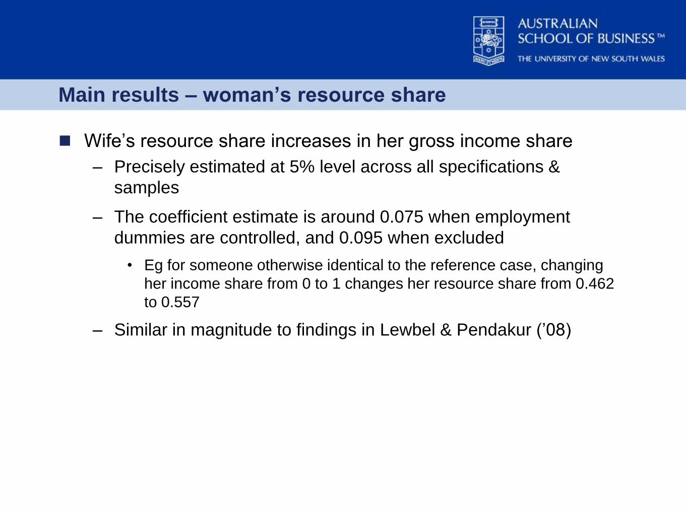
Main results – woman’s resource share
Wife‟s resource share increases in her gross income share
– Precisely estimated at 5% level across all specifications &
samples
– The coefficient estimate is around 0.075 when employment
dummies are controlled, and 0.095 when excluded
• Eg for someone otherwise identical to the reference case, changing
her income share from 0 to 1 changes her resource share from 0.462
to 0.557
– Similar in magnitude to findings in Lewbel & Pendakur (‟08)

Main results – woman’s resource share
Wife‟s resource share decreases in own disability and increase in
spousal disability
– In ‟04 and ‟05 sample, own disability reduces her resource share
by 0.05~0.06 and spousal disability increases it by 0.07~0.09
– The point estimates tend to be marginally in/significant at 10%
level
– In ‟04 and ‟07 sample, both own (-0.04~-0.05) and spousal
disability (0.04~0.06) effects somewhat smaller in magnitude,
though they are usually significant at 10% level and occasionally
at 5% level
Other demographic variations in resource share do not exhibit
robust patterns

’04-’05 Woman’s resource share, 11 goods
Intercept repreresents woman‟s resource share in the reference
household
Est S.E. Est S.E. Est S.E.
intercept 0.5234** 0.1019 0.5213** 0.0820 0.435** 0.0783
fem_shr 0.0779** 0.0364 0.0936** 0.0294 0.095** 0.0284
fem_age -0.0002 0.0020 -0.0006 0.0020 -0.0017 0.0021
man_age -0.0003 0.0016 -0.0005 0.0016 -0.0008 0.0015
fem_work -0.0026 0.0248
man_work -0.0345 0.0210
fem_educ -0.0335 0.0236 -0.0337 0.0243
man_educ 0.0080 0.0263 0.0936** 0.0294
fem_dis -0.0589* 0.0350 -0.0509 0.0356 -0.0492* 0.0292
man_dis 0.076* 0.0456 0.085* 0.0455 0.0690 0.0475
# parameters
# obs.
Specification 1 Specification 2 Specification 3
259 213 167
2051 2051 2051

’04-’07 Woman’s resource share – 11 goods
Est S.E. Est S.E. Est S.E.
intercept 0.4674** 0.0699 0.4783** 0.0671 0.4162** 0.0582
fem_shr 0.0835** 0.0250 0.0923** 0.0200 0.0996* 0.0210
fem_age 0.0005 0.0699 0.0013 0.0015 0.0003 0.0016
man_age 0.0005 0.0009 0.0007 0.0008 0.0002 0.0094
fem_work -0.0014 0.0202
man_work 0.0543** 0.0177
fem_educ 0.0010 0.0236 -0.0029 0.0101
man_educ -0.0036 0.0115 0.0016 0.0150
fem_dis -0.0461** 0.0213 -0.0328* 0.0195 -0.0375 0.0341
man_dis 0.0543* 0.0317 0.0663* 0.0348 0.0396* 0.0209
# parameters
# obs. 3971 3971 3971
Specification 1 Specification 2 Specification 3
259 213 167

Main results – economies of scale
Economies of scale parameters have been imprecisely estimated
in general
To be consistent with underlying structural interpretation, the
estimated scale must lie between 0.5 (all goods are jointly
consumed) and 1 (all goods are privately consumed)
For the reference wife, the scale estimate ranges from 0.48 to
0.67
For the reference husband, the scale estimate ranges from 0.41
to 0.74
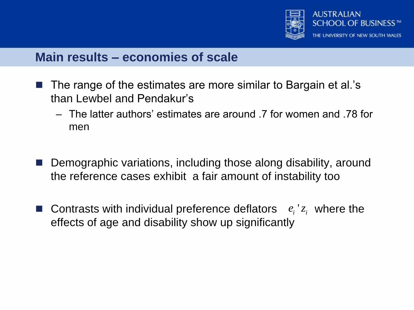
Main results – economies of scale
The range of the estimates are more similar to Bargain et al.‟s
than Lewbel and Pendakur‟s
– The latter authors‟ estimates are around .7 for women and .78 for
men
Demographic variations, including those along disability, around
the reference cases exhibit a fair amount of instability too
Contrasts with individual preference deflators where the
effects of age and disability show up significantly
'i ie z

’04-’05 log scale estimates : 11 goods
Intercept represent reference person‟s log scale economy
Est S.E. Est S.E. Est S.E
fem_intercept -0.7272* 0.3818 -0.4805* 0.2912 -0.9295** 0.3807
fem_age -0.0242** 0.0124 -0.0193* 0.0114 -0.0391** 0.0140
fem_educ -0.0613 0.2121 -0.0050 0.2016
fem_work 0.1217 0.1949
fem_dis 0.1214 0.2935 0.0615 0.2810 0.0735 0.3108
man_intercept -0.5006 0.3754 -0.5485* 0.3094 -0.2363 0.2409
man_age -0.0019 0.0124 -0.0053 0.0124 0.0022 0.0111
man_educ -0.0655 0.2570 -0.0252 0.2513
man_work 0.1059 0.2644
man_dis 0.1383 0.3255 0.0317 0.3132 0.1376 0.2813
… … … … … … …
# parameters
# obs. 2051 2051 2051
Specification 1 Specification 2 Specification 3
259 213 167

’04-’07 log scale estimates : 11 goods
Est S.E. Est S.E. Est S.E
fem_intercept -0.7356** 0.3603 -0.882** 0.3934 -0.9533** 0.3195
fem_age -0.0141 0.0101 0.0015 0.0118 -0.0113 0.0126
fem_educ -0.0613 0.2121 -0.1285** 0.0573
fem_work -0.05578** 0.0247
fem_dis -0.1601 0.2678 -0.1019 0.3020 -0.0624 0.3166
man_intercept -0.2912 0.2389 -0.2524 0.1977 -0.1492 0.1887
man_age 0.0145* 0.0076 0.0088 0.0080 0.0044 0.0095
man_educ 0.753** 0.2340 0.7184** 0.2381
man_work -0.1218 0.1634
man_dis -0.05178* 0.0238 0.2314 0.4325 0.04505** 0.0245
… … … … … … …
# parameters
# obs. 3971 3971 3971
Specification 1 Specification 2 Specification 3
259 213 167

Discussion
Due to overall instability of the scale estimates, difficult to answer
whether differences b/w spending patterns of couples w/ and
w/o disability can be partly explained by the economies of scale
Along with wife‟s income share, own and spousal disability are
found to influence her share of resources significantly
– In this study, the effect of disability has been estimated while
holding income share constant
– In practice, own disability may be accompanied by lower earnings
– Full impact of disability on intra-household resource allocations
may be bigger than what the point estimates suggest

Extensions?
A natural extension may be to concentrate on the issue of intra-
household resource allocations instead of analysing household
economies of scale at the same time
Have been recent advance in modeling approaches which
facilitate identification of sharing rules in a multi-person
household
– For example Dunbar, Lewbel and Pendakur (‟10)
– Allows to extend the scope beyond childless couples
– Doesn‟t require estimation of a full Engel curve system
• More robust estimates may be obtained

Theoretical framework
Due to Browning, Chiappori and Lewbel (unpublished, ‟09)
Assumes that the household behaves as if solving the following
program :
– μ = Pareto weight
– qf, qm = individual consumption vectors
– x = vector of purchased consumption goods
– A = matrix of household consumption technology
,max ( ) ( )
. . '
f m
f m
q q f m
f m
U q U q
s t p x y and q q Ax
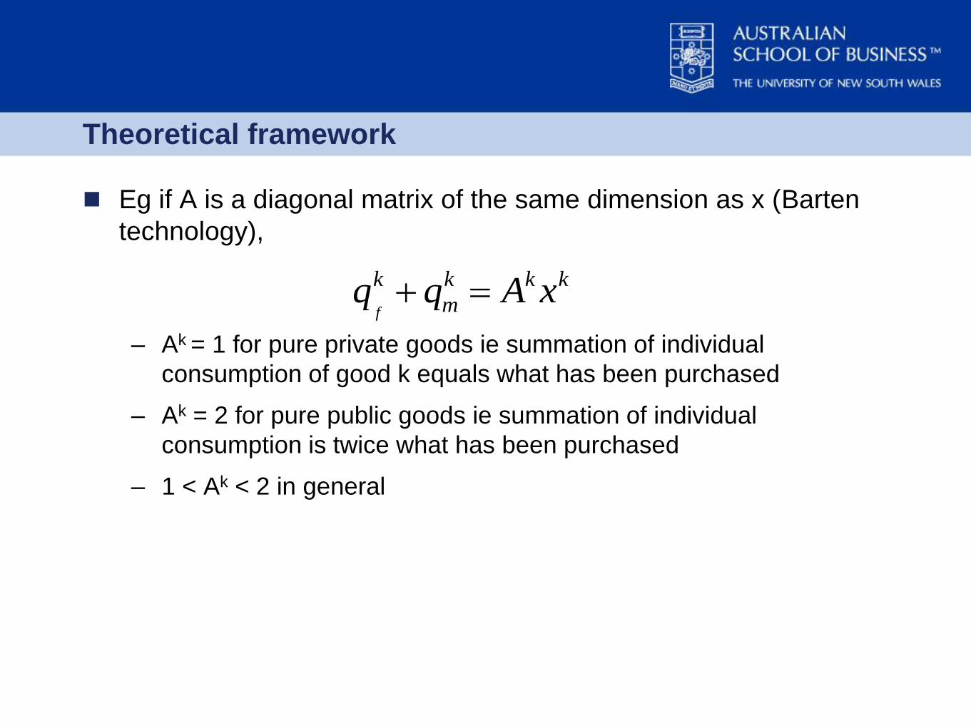
Theoretical framework
Eg if A is a diagonal matrix of the same dimension as x (Barten
technology),
– Ak = 1 for pure private goods ie summation of individual
consumption of good k equals what has been purchased
– Ak = 2 for pure public goods ie summation of individual
consumption is twice what has been purchased
– 1 < Ak < 2 in general
f
k k k k
mq q A x
Theoretical framework
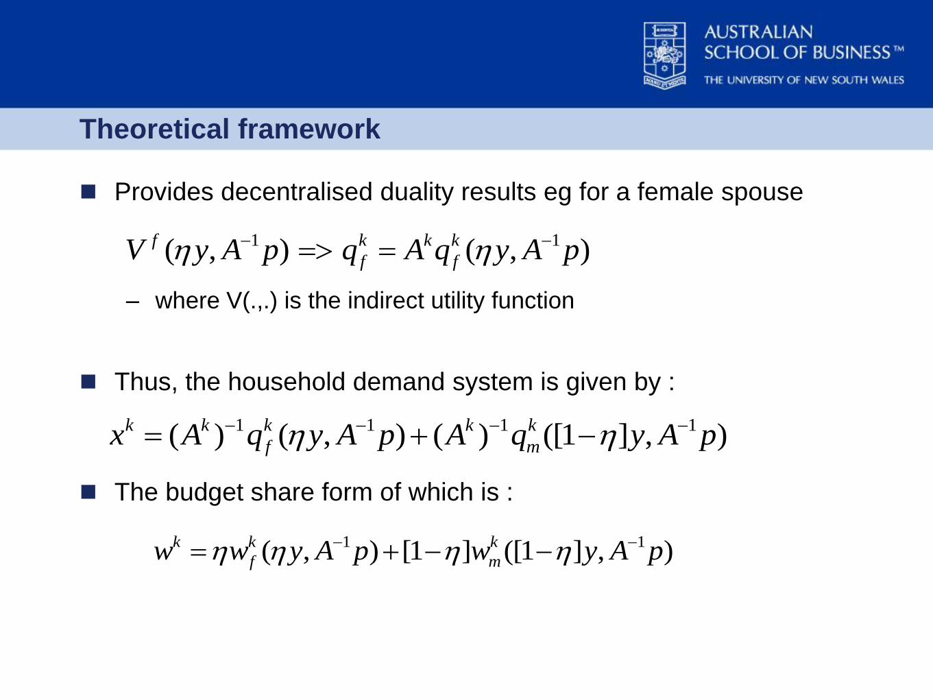
Provides decentralised duality results eg for a female spouse
– where V(.,.) is the indirect utility function
Thus, the household demand system is given by :
The budget share form of which is :
1 1( , ) ( , )f k k k
f fV y A p q A q y A p
1 1 1 1( ) ( , ) ( ) ([1 ] , )k k k k k
f mx A q y A p A q y A p
1 1( , ) [1 ] ([1 ] , )k k k
f mw w y A p w y A p

Theoretical framework
Estimation of a full BCL demand system requires a long span of
budget data and is computationally cumbersome
Lewbel and Pendakur (‟08) impose the following restriction on
preferences to transform the demand system into an Engel curve
system :
– ie there are budget deflators which can induce the same effect as
price deflators
1 1 [1 ]( , ) ( , ) & ([1 ] , ) ( , )f f m m
f m
y yV y A p V p V y A p V p

’04-’05 log scale estimates : 7 goods
Est S.E. Est S.E. Est S.E
fem_intercept -0.6947** 0.3554 -0.3928 0.2531 -0.7642** 0.3316
fem_age -0.0283** 0.0125 -0.0222** 0.0109 -0.0343** 0.0131
fem_educ -0.1351 0.1950 -0.1541 0.1819
fem_work 0.1054 0.1810
fem_dis 0.1823 0.2829 0.0845 0.2636 0.1206 0.2965
man_intercept -0.6125 0.3754 -0.8893** 0.3094 -0.4584 0.2860
man_age 0.0197 0.0124 0.0165 0.0146 0.0007 0.0139
man_educ 0.5122 0.3595 0.5287 0.3462
man_work 0.3594 0.2644
man_dis -0.2328 0.4545 0.0736 0.4323 -0.0586 0.3563
… … … … … … …
# parameters
# obs.
167 137 122
Specification 1 Specification 2 Specification 3
2051 2051 2051