An emissions inventory of air pollutants for the city of ...€¦ · Prof. Nestor Y. Rojas Grupo...
72
EIDGENÖSSISCHE TECHNISCHE HOCHSCHULE LAUSANNE POLITECNICO FEDERALE DI LOSANNA SWISS FEDERAL INSTITUTE OF TECHNOLOGY LAUSANNE An emissions inventory of air pollutants for the city of Bogotá, Colombia « Master Project 2010, Final Report » Advisors: Prof. Nestor Y. Rojas Grupo Interuniversitario de Calidad del Aire Universidad Nacional de Colombia, Bogotá, Colombia Prof. Alain Clappier LIVE – Laboratoire « Image Ville Environnement » Université de Strasbourg, France Prof. François Golay LASIG – Laboratoire des Systèmes d’Information Géographiques Ecole Polytechnique Fédérale de Lausanne, Suisse Master Candidate: Jan Philipp Robra Environmental Sciences and Engineering Program (SIE) School of Architecture, Civil and Environmental Engineering (ENAC) Swiss Federal Institute of Technology Lausanne (EPFL) June 2010
Transcript of An emissions inventory of air pollutants for the city of ...€¦ · Prof. Nestor Y. Rojas Grupo...

EIDGENÖSSISCHE TECHNISCHE HOCHSCHULE LAUSANNE
POLITECNICO FEDERALE DI LOSANNA
SWISS FEDERAL INSTITUTE OF TECHNOLOGY LAUSANNE
An emissions inventory of air pollutants for
the city of Bogotá, Colombia
« Master Project 2010, Final Report »
Advisors:
Prof. Nestor Y. Rojas Grupo Interuniversitario de Calidad del Aire
Universidad Nacional de Colombia, Bogotá, Colombia
Prof. Alain Clappier LIVE – Laboratoire « Image Ville Environnement »
Université de Strasbourg, France
Prof. François Golay
LASIG – Laboratoire des Systèmes d’Information Géographiques
Ecole Polytechnique Fédérale de Lausanne, Suisse
Master Candidate:
Jan Philipp Robra
Environmental Sciences and Engineering Program (SIE)
School of Architecture, Civil and Environmental Engineering (ENAC) Swiss Federal Institute of Technology Lausanne (EPFL)
June 2010


1
Abstract
More than 8.5 million people live in the urban area of Bogotá and more than
1.4 million vehicles are taking the road every day. Air pollution is becoming more and
more of a problem. Today, air pollution related respiratory diseases are the main
cause of death in young children in Bogotá and more than 6000 people die
prematurely every year in Colombia from cardiopulmonary diseases or lung cancer
related to air pollution.
The creation of a spatially and temporally distributed emission inventory with a
relatively high resolution for mobile and stationary sources (i.e. traffic and industries),
the subject of this thesis, is part of a bigger project aiming at the development of air
quality and meteorological modeling tools for the Secretaría Distrital de Ambiente,
Bogotá’s environmental agency. Five pollutants – carbon monoxide (CO), nitrogen
oxides (NOx), sulfur dioxide (SO2), particulate matter (PM) and volatile organic
compounds (VOCs) – are taken into account for the mobile sources, only four of
them – CO, SO2, NOx and PM – for the industrial sources. The sources are classified in
different categories and their emission factors determined before the calculated
emissions are distributed.
For the mobile sources, the emissions were calculated and distributed using the
EMISENS model developed jointly at the University of Strasbourg, France, and the
Swiss Federal Institute of Technology (EPFL) in Lausanne, Switzerland. A first attempt
was made using the program and some rough input parameters. The obtained results
and the uncertainty analysis included in the EMISENS model then allowed for a
precise focusing of the efforts that needed to be made to improve the results for the
second application of the model.
Concerning the stationary sources, the distribution in time was based on operational
information obtained from a field survey conducted by Universidad de los Andes and
the distribution in space on the street addresses of the manufacturing plant. All this
information was then represented graphically in ArcGIS®, enabling the visual analysis
of the results.
This study confirms an already known fact: the road traffic is responsible in most cases
for more than 90% of the emissions and all abatement strategies should focus on
these sources to be effective. The obtained quantities are close to the values given in
previous studies and the distribution in space and time showed in the first
comparisons good correlations with measured immission data.

2

3
Résumé
La population de la zone urbaine de Bogotá a atteint plus de 8.5 millions d’habitants
et chaque jour plus de 1.4 millions de véhicules circulent sur les rues de la ville. La
pollution de l’air pose de plus en plus de problèmes. Actuellement, les maladies
respiratoires liées à la pollution excessive de l’air sont la cause principale de décès
chez les jeunes enfants à Bogotá et chaque année plus de 6000 personnes meurent
prématurément en Colombie de maladies cardio-pulmonaires ou d’un cancer des
poumons en lien avec la pollution de l’air.
La création d’un cadastre d’émissions de polluants atmosphériques à relativement
haute résolution incluant les émissions des sources fixes et stationnaires (i.e. du trafic
et des industries) achevé dans ce projet fait partie d’un projet fait partie d’un projet
plus important visant à développer des outils de modélisation de la qualité de l’air et
de la météorologie pour la Secretaría Distrital de Ambiente, le service de
l’environnement de Bogotá. Cinq polluants ont été pris en compte pour les sources
mobiles, à savoir le monoxyde de carbone (CO), les oxydes d’azote (NOx), les
dioxydes de souffre (SO2), les particules en suspension (PM) et les composés
organiques volatils (COV). Pour les sources industrielles, seuls le CO, les NOx, le SO2 et
les PM ont été utilisés. Les sources ont ensuite été classifiées dans différentes
catégories et leurs facteurs d’émissions déterminés avant de distribuer les émissions
ainsi calculées dans la zone modélisée.
Les émissions des sources mobiles ont été déterminées à l’aide d’EMISENS, un modèle
de calcul et de distribution des émissions du trafic routier développé conjointement à
l’Université de Strasbourg, France, et à l’Ecole Polytechnique Fédérale de Lausanne
(EPFL), Suisse. Une première tentative de modélisation basée sur le programme et des
paramètres d’entrée très grossiers a été complétée. Sur la base des résultats obtenus
et de l’analyse des incertitudes incluse dans EMISENS, la redéfinition des paramètres
afin d’améliorer le modèle a pu se faire de manière très ciblée.
En ce qui concerne les sources fixes, la distribution temporelle s’est basée sur des
informations opérationnelles trouvées dans une étude de terrain menée par
Universidad de los Andes et la distribution spatiale sur les adresses des sites de
production. Toutes ces informations ont ensuite été représentées graphiquement
dans ArcGIS®, afin de pouvoir visualiser les résultats.
L’étude a confirmé un fait déjà connu : le trafic routier est responsable dans presque
tous les cas de plus de 90% des émissions et toutes les stratégies d’abattement
devraient donc se focaliser sur ces sources afin d’être effectives. Les résultats obtenus
sont proches des valeurs citées dans des études précédentes et la distribution
spatiotemporelle montre dans les premières comparaisons une bonne corrélation
avec les données d’immissions mesurées.

4

5
I. Table of Contents
Abstract ...........................................................................................................................................1
Résumé ............................................................................................................................................3
I. Table of Contents ..................................................................................................................5
II. List of Figures ...........................................................................................................................6
III. List of Tables ............................................................................................................................7
1. Introduction ............................................................................................................................9
2. Methodology ...................................................................................................................... 11
2.1. Definitions .................................................................................................................... 12
2.2. Modeled area and pollutants ................................................................................. 13
2.3. EMISENS ........................................................................................................................ 13
2.4. ArcGIS® ....................................................................................................................... 16
2.5. Data sources and preparation ............................................................................... 16
2.6. An iterative approach .............................................................................................. 17
3. Results and procedures ..................................................................................................... 19
3.1. The mobile sources: first attempt ............................................................................ 19
3.2. The mobile sources: improvement of the model ................................................ 26
3.3. The stationary sources: a third step ........................................................................ 34
3.4. Total Emissions ............................................................................................................. 38
4. Validation of the model: first insights .............................................................................. 42
5. Conclusions and Perspectives ......................................................................................... 45
6. Acknowledgments ............................................................................................................. 46
7. Bibliography ......................................................................................................................... 47
Appendixes .................................................................................................................................. 51
Appendix I : Description of the pollutants and their effects on health ........................ 53
Appendix II : Classification Diagram for the Vehicle Types in Bogotá based on
engine technology and size, adapted from (CIIA, 2008b) ............................................ 54
Appendix III : Base values for the emission factors (EF) used in this project, error
values (Err.) and sources ....................................................................................................... 55
Appendix IV : Mobile sources emission factors for the different pollutants, each
vehicle category and each road category of the first modeling attempt ................ 56
Appendix V : Proportioned flux data as used for the distribution in time in the first
application of the model ...................................................................................................... 58
Appendix VI : Map of the 20 localities composing the district of Bogotá ................... 59
Appendix VII : Maximum values for each category in the road survey ...................... 60
Appendix VIII : Results of the road survey data analysis ................................................. 61
Appendix IX : Illustration of the Thiessen algorithm .......................................................... 62
Appendix X : Mobile sources emission factors for the different pollutants, each
vehicle category and each road category of the second modeling attempt ........ 63
Appendix XI : Graphical analysis of the traffic distribution in time on the different
main road subcategories ...................................................................................................... 65
Appendix XII : Classification Diagram for the Industrial Categories in Bogotá based
on their technology and size, adapted from (CIIA, 2008a) ........................................... 67
Appendix XIII : Graphical representation of the hourly industrial sources emissions for
the pollutants considered in this project ............................................................................ 68
Appendix XIV : SO2 emissions from mobile sources at 08h00, based on the second
application of the model ...................................................................................................... 70

6
II. List of Figures
Figure 1: Typical inputs for Bottom-Up and Top-Down methodology adapted from
(Ntziachristos, Samaras, & al., 2009) ....................................................................... 15 Figure 2: Some of the road networks used in the first application of the model, the grid
has a spatial resolution of 1km2 ............................................................................... 20 Figure 3: Speed dependency of vehicular PM10 emissions for a EURO II Diesel car (DFT-
UK, 2010) ....................................................................................................................... 23 Figure 4: NOx Emissions at 07h00 calculated by the first application of the model, the
distribution in space shows some inconsistencies with local reality ................. 25 Figure 5: Graphical representation of the fraction of daily traffic for every hour and
vehicle category, mean value for the main roads ............................................. 31 Figure 6: NOx Emissions at 07h00 calculated by the second application of the model
....................................................................................................................................... 33 Figure 7: Comparison between the emissions (CO at 15h00) calculated by EMISENS
and the traffic charge defined on the main roads. The traffic charge is
symbolized in dark green for low traffic, light green for medium traffic,
orange for high traffic and red for the very high traffic. .................................... 33 Figure 8: Localization of the different industrial sources and limits of the localities
forming the northern part of the Bogotá district .................................................. 34 Figure 9: Graphical representation of the number of industrial sources active at the
same time .................................................................................................................... 36 Figure 10: Daily emissions of CO by the stationary sources considered in this report ... 37 Figure 11: Daily emissions of PM by the stationary sources considered in this report ... 38 Figure 12: Filters used to measure PM emissions; on the left, a filter used in a coal fired
plant, on the right, a filter from a natural gas fired plant (CIIA, 2008a) .......... 38 Figure 13: Total CO emissions at 08h00, combining emissions from mobile and
stationary sources....................................................................................................... 39 Figure 14: Total NOx emissions at 08h00, combining emissions from mobile and
stationary sources....................................................................................................... 40 Figure 15: Total SO2 emissions at 08h00, combining emissions from mobile and
stationary sources....................................................................................................... 40 Figure 16: Total PM emissions at 08h00, combining emissions from mobile and
stationary sources....................................................................................................... 41 Figure 17: VOC emissions from the mobile sources only, no emissions calculated for
the stationary sources ............................................................................................... 42 Figure 18: Monitoring results for immissions measured by the RMCAB station in
Kennedy, the measures are given in [µg/m3] for every hour ............................ 43 Figure 19: PM emissions and wind direction around 07h00 in the morning ; the stars
indicate the approximative localization of the monitoring stations Fontibón
(in the north) and Kennedy (in the south) ............................................................. 43 Figure 20: on the right, total PM emissions at 08h00 the darker the color, the higher the
emissions (produced for this project); on the left, PM10 yearly mean
concentrations as compared to the legal limit, white represents lower values
and red represents higher values (Behrentz, 2007) ............................................. 44 Figure 21: grey lines connect all the points of an input dataset, red lines define the
boundaries of the polygons using a Thiessen method (source: www.ems-
i.com) ............................................................................................................................ 62

7
III. List of Tables
Table 1: Total length of the road segments in the different road categories, first
attempt ........................................................................................................................ 20 Table 2: Estimated vehicle speeds on the different road categories, first attempt
(except for Transmilenio, average velocity) ......................................................... 21 Table 3: Vehicle categories data (sources – (CIIA, 2008b), except the italic values
provided by Transmilenio S.A., all have been regrouped and the activities
determined in this project) ....................................................................................... 21 Table 4: Percentage of total daily covered distance on the different road categories,
first application of the model................................................................................... 22 Table 5: Activities of the mobile sources distributed among the different road
categories of the first attempt in [veh*km/h] ....................................................... 22 Table 6: Standard deviation of the different parameters in percent .............................. 23 Table 7: The results of the first application of the model exceed by far the results of
(CIIA, 2008b) ................................................................................................................ 26 Table 8: Standard deviation values in percent for the emission factors and hourly
street mileage for vehicle category VP_CC and road category SEC for the
five pollutants considered for the mobile sources ............................................... 26 Table 9: Total length of the road segments in the different road categories and
subcategories, second attempt ............................................................................. 27 Table 10: Average velocities on the different road categories for the second
application of the model, no distinction is made according to the traffic
charge, thus all main road (PRINC) and secondary road (SEC) categories
have the same velocity values and are not presented separately. A velocity
of 0 [km/h] means that this vehicle category is not present on the roads of
this category. .............................................................................................................. 28 Table 11: Maximum traffic values (number of vehicles in one hour) for each vehicle
category and on each main road subcategory. The last row represents the
total of the maxima for each vehicle category. ................................................. 29 Table 12: Percentage driven on each main road category and for each vehicle
category ...................................................................................................................... 29 Table 13: Secondary road classification factors based on the road length .................. 30 Table 14: Average hourly street mileage, values for the newly created subcategories
on main and secondary roads ................................................................................ 30 Table 15: Standard deviation for the different parameters, in percent .......................... 31 Table 16: Comparison of the results of the second application of the model with the
results from previous studies, adapted from (CIIA, 2008b) ................................. 32 Table 17: Emission factors grouped by category (gas fired boilers CG1, CG2 and CG3;
gas fired ovens HG; coal fired boilers CC1 and CC2; coal fired ovens HC;
coal fired brick burning kilns HL; equipment using liquefied petroleum gas
GPL, diesel D, or used vegetal oil AU). ................................................................... 35 Table 18: Annual emissions calculated for the industrial sources; the extrapolated
values try to take into account the sources presenting insufficient data (242
sources out of 1478, i.e. 16.37 %) and comparison with values presented in
(CIIA, 2008a) ................................................................................................................ 36 Table 19: Influence of the different sources on the final result .......................................... 39

8

9
1. Introduction
As described in the United States Environmental Agency’s (US-EPA) “Handbook for
Criteria Pollutant Inventory Development”: an emission inventory is a current
comprehensive listing, by source, of the air pollutant emissions, and covers a specific
geographic area for a specific time interval. The same handbook also states: emission
inventories are used for a wide variety of purposes, but are most often developed in
response to regulation. Emission inventory data are used to evaluate the status of
existing air quality as related to air quality standards, air pollution problems, assess the
effectiveness of air pollution policy, and initiate changes as needed. Emission
inventories provide the technical foundation for programs designed to improve or
maintain ambient air quality. They are used to identify sources and general emission
levels, patterns and trends, to develop control strategies and new regulations, and
serve as the basis for modeling of predicted pollutant concentrations in ambient air
(EPA-OAQPS, 1999).
One of the big problems related with air pollution are its effects on health and the
environment. The pollutants covered by the inventory presented in this report –
namely carbon monoxide (CO), nitrogen oxides (NOx), sulfur dioxide (SO2),
particulate matter (PM) and volatile organic compounds (VOCs) – are all part of
US-EPA’s list of criteria pollutants defined by the Clean Air Act (CAA, 2004) or serve as
precursors for these pollutants. These pollutants are responsible for the formation of
acid rains and ozone, impact aquatic and terrestrial ecosystems and all of them
show effects on human health. They can reduce the delivery of oxygen to organs
and tissues, irritate the lungs, cause bronchitis and pneumonia, lower the resistance to
respiratory infections and increase the likeliness of suffering from cardiopulmonary
diseases or lung cancer (EPA-OAQPS, 1999). A broader description of their properties
and effects on health can be found in Appendix I.
Bogotá, Colombia’s capital and biggest city of the country, is situated on the highest
plateau in the Colombian Andes, the Sabana, amidst a mountain formation in the
east, the Rio Bogotá in the west and a hillier region in the south. The city’s elevation is
more than 2600 m above MSL, although further east, to the Llanos, and west, towards
the Rio Magdalena, some kilometers away from the city, the altitude decreases
rapidly to almost sea level. Bogotá has a subtropical high-mountain climate and an
annual average temperature close to 14°C – most of the time between 5°C and
25°C. Along with this very constant temperature, only two seasons coexist: the wet
season and the dry season. Most of the rains occur during the months of April, May,
September, October and November; the remaining months of the year being rather
dry. The capital district is composed of 20 localities of different sizes and different
main soil uses. Mainly rural on the outskirts, the commercial activities are
concentrated in the eastern part of the city center and most industrial sites
are located in the western central part of the city. The poorest areas of the city are
situated in the south, where most of the displaced people, fleeing the guerrilla and
other armed forces in the rural parts of the country, have settled. It is estimated that in
Colombia almost 72% of the population, or 32 million people, live in urban

10
areas (Sánchez-Triana, Kulsum, & Yewande, 2007). In 2009, Bogotá’s population had
risen to an estimated 7.26 million inhabitants, based on the official projections from
the national census 2005 (DANE, 2005), and the estimations for the whole urban area
are actually much higher, accounting for more than 8.5 million inhabitants.
One of the major environmental and health related concerns in Bogotá is air
pollution, as the amount of engine powered vehicles continues to rise. At present,
there are more than 1.4 million cars on the roads every single day. The average age
of the vehicle fleet in Bogotá is relatively high. For buses, for example, estimations are,
that the average age is close to 15 years and maintenance rather poor (Echeverry,
Ibáñez, & Hillón, 2004). Efforts are made to reduce actual and potential impacts.
Politicians and the public become more and more aware of the problem, new
policies are put in place, public collective transportation systems are developed
(« Transmilenio », a rapid mass transport system using buses circulating in their own
lanes; a subway is projected) and circulation restrictions (« Pico y Placa ») apply to
privately owned vehicles used for individual or collective transportation (SDM, 2010).
The recent quality increase of diesel combustibles used in Bogotá – a progressive
reduction of the sulfur concentration from 1200 ppm to 50 ppm – is yet another factor
reducing significantly harmful emissions (SDA, 2010). Still, according to the World
Bank’s world development indicators, Bogotá’s air counts among the 50 most
polluted in the world (World Bank, 2007), but the situation is improving. The quality of
life in Bogotá, as measured by the consulting firm Mercer, which includes air quality
as a parameter, has improved compared to the earlier measurements. In the actual
ranking, Bogotá is situated at the 132nd place out of 221 investigated cities, two
places better than the previous year (Mercer, 2010).
The relations between air pollution and respiratory diseases have been evaluated in
several studies conducted in Bogotá. In a risk assessment, it has been established that
annually approximately 2’300 premature deaths due to cardiopulmonary diseases
and lung cancer can be attributed to long term PM2.5 exposure and close to 1400
premature deaths to short term PM10 exposure in Bogotá alone (Llorente Carreño,
2009). The same study also found that a reduction of PM10 concentrations by 30%, as
it might be induced by an extension of the Transmilenio network, would result in an
annual avoidance of close to 400 premature deaths in Bogotá. The reduction of the
sulfur content in diesel fuels is yet another possibility studied in this report, which
suggests that a reduction of the sulfur content from 1000 to 500 ppm would avoid
annually more than 750 premature deaths. As stated above, in Bogotá, the sulfur
content just was reduced to a maximum of 50 ppm (SDA, 2010).
Emission inventories have been realized at various times for the city of Bogotá. One of
the first studies on this subject was done by the Japan International Cooperation
Agency between 1990 and 1992 (JICA, 1992), followed several years later by studies
financed by the Departamento Técnico Administrativo del Medio Ambiente (DAMA),
which later became the Secretaría Distrital de Ambiente (SDA) – Bogotá’s
environmental agency. These informations were included in the “Plan de gestión del
aire para el Distrito Capital 2000-2009”, published by the DAMA in 2001. In 2002, in

11
one of the latest attempts in this subject, Universidad de los Andes (UniAndes) applied
the AIREMIS model (ACRI-ST, 2002) for the city of Bogotá (Zárate, Belalcázar, Clappier,
Manzi, & Van den Bergh, 2007).
Standards for the determination of emission inventories for traffic are numerous. In
Europe, mainly two methodologies coexist: the HBEFA, the Handbook of Emission
Factors, developed jointly by Germany, Switzerland and Austria (HBEFA, 2010) and
the European COPERT IV methodology (COPERT IV, 2010) used in the EMEP/CORINAIR
Emission Inventory Guidebook (EMEP/CORINAIR, 2009). European projects, like
ARTEMIS (André, Keller, Sjödin, Gadrat, & Mc Crae, 2008) try to unify these different
methodologies in a single tool to model all traffic related emissions.
The project presented in this report is part of a research mandate for the SDA and
Ecopetrol, Colombia’s principal petroleum company, at the Universidad Nacional de
Colombia in Bogotá (UNAL). It follows earlier investigations led by UniAndes, who
determined emission factors for key pollutants of the car fleet (CIIA, 2008b) as well as
the major industries (CIIA, 2008a) in the capital city Bogotá and produced an
updated emissions inventory based on these factors, but without a focus on spatial
and temporal distribution.
The main objective of the present project was to produce an air pollutants emissions
inventory which does specifically include a distribution in time and space for the
mobile and stationary sources (e.g. traffic and industries) based on the EMISENS
model. This tool was developed jointly by and is still in development at the University
of Strasbourg and the Swiss Federal Institute of Technology in Lausanne, EPFL (LIVE,
2010). Additionally, the usability of the tools as well as the quality of the available
data needed to be evaluated and missing data identified for future applications of
the model. A second objective, but not less important, was the capacity building in
Colombia. A great part of the knowledge had to be transmitted to the partners in this
project, thus enabling them to be autonomous for future applications based on the
tools and theories used. In this project, pollutant transport or reactions are not
considered, only emissions.
The research mandate ultimately aims at an actualization of the meteorology and air
quality models for Bogotá, which will not only model the different emissions, but also
transport and reactions of the contaminants, to help support political decision
making in the next years and tackle effectively the air pollution problem of the city.
2. Methodology
Some useful definitions for a better understanding of the methodology and theory
used in this project are presented in the following section. A reader who is familiar
with the subject of this report may directly jump to chapter 2.2.

12
2.1. Definitions
Stationary sources
Stationary sources are emission sources, mainly caused by industrial or artisanal
activities. They are often called point sources, because their emission can be
quantified and allocated to a single point of emissions, for example the stack of an
industrial installation.
Mobile sources
The mobile sources include all traffic related emissions, i.e. the emissions produced by
the vehicles circulating in the area that is studied.
Hot emissions Hot emissions are the emissions produced by the combustion while the equipment is
already at normal working temperature, meaning the functioning is already stabilized
(Kennesaw State University, 2006).
Cold emissions Cold emissions are the amount of additional emissions that are emitted while the
equipment is not yet at the normal working temperature. Emissions for some
pollutants are higher if the temperature of the equipment and mainly its emissions
control equipment is lower than its optimal operating temperature (Kennesaw State
University, 2006).
Evaporative emissions These emissions concern mainly the volatile organic compounds (VOCs) emissions.
They occur in four different ways: “running losses”, meaning the amount of fuel
evaporated while the engine is running; “hot soak”, or evaporation while the engine
is off but still warm; “diurnal emissions”, occurring while the car is parked and the
engine is cool due to the external temperature; and finally “refueling”, losses
occurring while the tank of the vehicle is being filled (Kennesaw State University,
2006).
Emission factor The emissions of the different sources can be measured and transformed in emission
factors for each pollutant, meaning the amount of the considered pollutant emitted
every kilometer for the mobile sources or every hour for the stationary sources. Those
factors are, for example, speed and temperature dependent for the mobile sources.
Vehicle type Vehicles presenting similar engine technologies and using the same fuel type are
grouped as being the same type of vehicles. Thus, the emission factors are the same
for all the vehicles of one given type.
Vehicle category Vehicle types presenting the same behavior on the road are grouped in a single
category. Each category then contains vehicles of different types and thus different
emission factors. Even though, single emission factors can be derived for each

13
category by using the number of vehicles in each type and the total amount of
vehicles in the respective category to aggregate the type emission factors weighted
by their relative importance. This can be expressed by the equation 1:
∑
Where F is the emission factor for the category c or the type of vehicle t, nc the
amount of vehicles in the considered category, nt the amount of cars for each type
and j the number of different vehicle types in category c.
Road category The entire road network is divided in categories based on a similar vehicle velocity
and traffic load, for example. Roads classified in the same category are grouped
together and treated in the same way for the calculations with EMISENS.
Activity
For the mobile sources, e.g. the road traffic, the activity represents the hourly
distance covered by all the vehicles in a same vehicle category and on the same
road category in [veh*km/h]. The activity of the stationary sources is equivalent to the
fuel consumption, i.e. an amount of fuel in kg, l or m3 burned during a defined interval
of time, in our case every hour.
Grid and Cells The grid represents a subdivision of the square sized area to be modeled in individual
equal sized cells. It is a “rasterization” of the actual area in order to simplify the
calculations.
2.2. Modeled area and pollutants
The inventory produced in this project is a spatial and temporal distribution of the
emissions calculated for the city of Bogotá for a typical day. The emissions are thus
distributed over a grid of 55 km by 55 km centered over the city area of Bogotá and
with a spatial resolution of 1 square kilometer. Values are calculated for every cell
and hour of the day (i.e. 55 x 55 = 3025 cells and 24 hours).
Two categories of emission sources are taken into account for this project: mobile
sources, meaning the road traffic; and stationary sources – mainly industrial boilers
and ovens. These sources represent the lion part of the anthropogenic emissions for
the contaminants considered in this report: carbon monoxide (CO), nitrogen oxides
(NOx), sulfur dioxide (SO2), particulate matter (PM), and – for the mobile sources only –
the volatile organic compounds (VOCs).
2.3. EMISENS
The emissions produced by the mobile sources are calculated and distributed in
space and time using the EMISENS model. The EMISENS model is developed to
address main difficulties developing countries face while trying to confront the ever

14
increasing air pollution problem coupled with their strong economic growth. These
difficulties include the complexity of the data needed for the classic traffic emission
models and the computing power needed to obtain the results based on road
segment modeling. Sufficient data is not always available to use models like
CIRCUL’AIR, in use in several French departments and developed by the ASPA, the
“Association pour la Surveillance et l’Étude de la Pollution Atmosphérique en Alsace”,
and which requires very detailed input information (Schillinger, 2008) or AIREMIS
(ACRI-ST, 2002), which has been used in Bogotá earlier (Guéguen, Zarate, Mangin,
Clappier, & Sanchez, 2003). Moreover, powerful computers, which enable dealing
with the great amount of calculations involved in the elaboration of emission
inventories using other programs in a reasonable time frame, are only available at
mostly prohibitive costs for local institutions in developing countries.
Another limiting factor is that most of these models do not integrate uncertainties
computation. EMISENS is able to produce results without the need for very complex
information. Instead of differentiating each road segment and the associated
vehicles and emission factors, this information is aggregated in larger categories and
average values are used for the relevant parameters. This “grouping” of information
produces a very important gain in the amount of calculations needed to obtain the
results and allows for uncertainty analysis of the results with respect to the input
parameters and their respective error values using the Monte Carlo methodology. This
enables the user to identify the parameters that should be revised with priority in order
to obtain a significant improvement of the results (LIVE, 2010).
EMISENS can be used within a wide range of levels of complexity. The calculations
can be done using solely “hot emissions”, meaning the emissions produced while the
engine is already warm/hot. It is possible to determine the “cold emissions” or “over
emissions”, produced while the engine is still cold during a certain period after the
initial ignition. Even the “evaporative emissions”, emissions not caused by the
combustion itself, are planned to be included in a near future. As well as many other
programs used to elaborate emission inventories, EMISENS is based on the COPERT IV
methodology to estimate emission factors for the different car categories and types
of emissions. As already stated, the main difference with other emission inventory
elaboration techniques lies in the grouping of the different types of vehicles in
categories of similar behavior and roads in categories based on speed and traffic
charge.
Another important difference with most of the other programs is the bottom-up and
top-down consistency achieved with EMISENS. Mostly, the results obtained using
these two approaches differ in a more or less significant way from each other. The
top-down approach first estimates a global value without considerations for the
single entities before refining the results by distributing them over the area to be
modeled. The bottom-up approach looks at the problem the other way round and
considers first the single emissions to finally combine them in the last step and obtain
the global emissions. Typical input parameters for the two approaches are found in
Figure 1.

15
Figure 1: Typical inputs for Bottom-Up and Top-Down methodology adapted from (Ntziachristos,
Samaras, & al., 2009)
EMISENS is able to combine favorably both approaches. It has the ability to calculate
in a first step the global emissions in the studied area using a top-down approach
and then, using a bottom-up methodology, distribute these emissions in space and
time. The consistency between the two approaches is ensured by the formulation of
the emissions in EMISENS, based on equation 2:
∑
Where E are the emissions in [gr/h], F the emission factors for the different sources in
[gr/unit] and A their respective activities in [unit/h]. The emission factors are average
values and mostly derived using a top-down methodology, whereas the activities are
local values often based on a bottom-up approach. If the emission factors used are
constant in space and time, the total emissions obtained by the top-down approach
or the bottom up approach will be the same and thus insure the coherence between
the two methods.
EMISENS is usually used in three distinct phases. The first step consists in an estimation
of the total emissions based on the least input parameters needed, meaning the
emission factors and the activities for each road and car category. The second step
takes into account the error values for these input parameters to compute their
relative influence on the uncertainties of the results. Finally, the third step needs some
extra information, like road network and traffic charges for every cell and every hour
of the model’s domain, to be able to distribute the emissions in space and time.
The EMISENS tool has been validated by comparing its results with the results
produced by the CIRCUL’AIR tool, based on a bottom-up methodology, over the city
Bottom-Up Methodology
Input Activity Data
- Traffic counts
- Vehicle composition
- Speed recordings
- Length of roads
- Area knowledge
Input emission data
Emission and fuel
consumption factors
(speed dependent or
speed/acceleration
dependent)
Top-Down Methodology
Input activity data
- Vehicle park and
composition
- Fuel consumption
- Representative speeds
- Country balances
Input emission data
Emission and fuel
consumption factors
(average representative
or speed dependent)

16
of Strasbourg, France. The differences between the two models were relatively small.
This test also proved the ability of EMISENS to produce valid results not only for
developing countries, where the focus is a little less on precision than on the ability to
obtain results, but also for countries which expect a much higher resolution or
precision of the results (Ho, 2010).
2.4. ArcGIS®
The principal software used in this project to prepare the input data for EMISENS and
represent graphically the results was ESRI®’s ArcGIS® in its ArcInfo® version, which
includes the most complete set of functionalities and tools available. ArcGIS® was
used to produce the grid, calculate the lengths of the road segments of each road
category and for every cell of the grid. The data tables associated with the different
data sets were used to produce the input data needed for the EMISENS model.
Finally, ArcGIS® was also used to produce the graphical illustrations of the emissions
calculated with EMISENS for every hour of the day and other maps of the modeled
area around Bogotá presented in this report.
2.5. Data sources and preparation
For this project, the input data used was obtained from different sources. The emission
factors were mainly found in the two final reports of the project led by UniAndes (
(CIIA, 2008a) and (CIIA, 2008b)) and complemented by COPERT IV values (COPERT
IV, 2010) if no data was available for the mobile sources or EPA/AP-42 data for the
stationary sources (EPA, 2010). The different vehicle categories, number of vehicles in
each category, as well as the daily distances covered by the different vehicles were
found in the same reports and complemented by data from the company operating
the Transmilenio system (Transmilenio SA). The data for the primary and secondary
road network was obtained through the SDA, as well as the soil use classification and
the limits of the different localities. The Transmilenio network data was provided by the
Research Program in Traffic and Transport (Programa de Investigación en Transito y
Transporte – PIT) of the UNAL. The data for the stationary sources was obtained from
the SDA as files produced by UniAndes for their inventory elaboration. The traffic
survey data for the primary roads was obtained from the Secretaría Distrital de
Movilidad (SDM). Finally, the rural roads – meaning the roads that are not in the
Bogotá district, which is more or less equivalent to the urban area – were obtained
from the MapInfo® files used in the preceding project led by UniAndes.
Following a closer examination of the different datasets, it appeared that some
needed to be reworked, before they could be used as input data for the project.
Some data sets did not include a correct geo-reference and thus needed to be geo-
localized beforehand; others were not useable directly due to faulty data or included
data that was out of range, as described in the following paragraphs.
The stationary sources data, for instance, required a very detailed manual
verification, because most of the sources needed to be correctly re-located. The
average distance between the same locations in the old and in the corrected

17
versions was about 600 meters, but some sources were found to be located almost 10
kilometers away from their correct location.
The secondary road network needed some preliminary treatment as well. The two
files received included one specifically for the primary roads and a second file which
represented the whole road network of Bogotá. In order to be able to use these files,
the duplicate primary roads needed to be removed from the file representing the
complete road network, so that only secondary roads remained in this file.
The primary roads network received included some road segments that were only
planned and not yet constructed at the moment of the project and which had to be
removed. Additionally, some existing primary roads were missing in this file and had to
be added manually.
The MapInfo® files did cover an area much larger than the modeled area in this
project and included some primary roads as well. The roads out of the modeled area
as well as the ones located within the Bogotá district area had thus to be removed in
order to keep only the roads out of the district boundaries but still inside of the
considered area.
The preparatory phase included also the construction of the model grid in order to be
able to calculate values for the different elements that are considered for every cell
of the grid. The grid was prepared using the “Fishnet” tool available in ArcGIS®. This
tool requires the entry of the coordinates of the lower-left and upper-right corner of
the area to be covered by the grid, the size of the cells (1km x 1km) and the number
of rows (55) and columns (55) to be produced. The option to produce numbered
labels for every cell was used to obtain a sequence of numbers (numbering the cells
row by row from the bottom-left cell, number 0, to the top-right cell, number 3024)
which was then converted to X and Y coordinates as used in EMISENS (ranging each
from 1 to 55, the origin being the lower-left corner). This transformation was done
using the following mathematical formulas (equation 3 and 4) and the “calculate
values” tool in ArcGIS®.
Where X and Y are the coordinates to be determined, Id is the number of the cell
label, 55 the number of cells in each row, mod the modulo operator and “\” the
integer division as used in Visual Basic (VBA).
2.6. An iterative approach
Regarding the mobile sources, the input parameters were defined twice. The first set
of parameters used many estimated values and a very rough subdivision of the road
networks, whereas the input parameters were substantially refined for the second set,
according to the first results. This iterative approach was chosen mainly for two
reasons: 1) the necessary level of detail for the input parameters needed in order to

18
obtain satisfactory results was unknown; and 2) due to the unavailability of some of
the input parameters it was necessary to estimate them. The validation of the values
chosen for those parameters was done based on the results of the different
applications of the model.
The main objective of the first application of the model was to verify that all the tools
needed were working correctly and to evaluate which parameters had the biggest
influence on the emission results, what needed to be evaluated more precisely and
what information was missing and needed to be obtained. Since not all the data
were yet available at the time, some input parameters were based on estimations
done by people having sufficient local knowledge (e.g. living in the neighborhood,
etc.). The results produced by this first modeling attempt were then represented
graphically and summarily analyzed.
Following the analysis of the results of the first attempt, new input data were prepared
for a second application of the model, using newly available and more precise data,
where possible. By focusing the improvement efforts on the factors, which the
uncertainty analysis included in EMISENS had indicated as having the greatest
influence on the final result, the execution of the ensuing steps was quite
straightforward.
In a third step, the emissions of the stationary sources, i.e. the industrial emissions, were
calculated. These sources included industrial ovens and boilers running on fuels as
diverse as natural gas, liquefied petroleum gas, coal, diesel or used vegetal oil. The
emissions were calculated for every single source and, in a subsequent step, all the
emissions from sources located in the same cell added to produce similar results than
for the mobile sources: emissions distributed over a grid of 3025 distinct cells of 1km2
and every of the 24 hours of a day.
Both results – from the second application of EMISENS for the mobile sources and the
results for the stationary sources – were finally combined in ArcGIS® to produce a
cadaster for all the emissions considered in this project. This was done by adding the
values pollutant by pollutant in order to obtain the total emissions for each cell of the
grid (Equation 5).
Where p is the pollutant considered, Emov are the mobile sources emissions in cell (i,j),
Efix the stationary sources emissions in cell (i,j) and Etot represents the total emissions in
cell (i,j).
As a last step, these results were compared to existing measurement data in order to
validate or not the results of this project. This comparison was done mostly
qualitatively, based on the PM emissions evaluated with the model and the
immissions measured by the air quality monitoring network of Bogotá.

19
3. Results and procedures
The respective results for the mobile sources are presented in separate chapters (3.1
and 3.2). Another chapter (3.3) presents the results for the stationary sources emissions
and, finally, the last chapter (3.4) the combined emissions of both types of sources. In
all these chapters, the techniques applied to define the input parameters used in the
different steps of the modeling procedure are explained in separate subchapters. At
the end of each chapter, the results are evaluated based on the spatial and
temporal distribution that was produced. The analysis of the final results is presented
as a separate chapter (chapter Error! Reference source not found.).
The images of the emissions cadaster presented in this report will only be for hours where
peak emissions take place. This is mainly due to the huge amount of graphical material
that was produced – more than 500 different images, representing the emissions of the
mobile sources, the stationary sources and both sources combined for each of the 24
hours of a day and every one of the 5 pollutant considered in this report. The complete
set of graphical representations of the results, the different numerical results, as well as
some animations of the results are included on a CD-ROM attached to this report.
3.1. The mobile sources: first attempt
During this attempt, the functioning of all the used tools was verified and the needed
parameters defined as a first approximation. The values chosen for the different input
parameters and how they were obtained are explained in the following subchapters.
3.1.1. Vehicle categories
The vehicle fleet in Bogotá was already completely characterized during the project
led by UniAndes (CIIA, 2008b). The vehicles were subdivided into different categories
based on the type of vehicle, their engine technology and capacity. This resulted in a
total of 23 different categories: 4 for cars, 4 for four wheel drive vehicles (4x4) and
small vans, 2 for the taxis, 2 for the buses, 1 for the micro-buses, 1 for the school and
touristic buses, 3 for the trucks, 1 for the articulated Transmilenio buses, 1 for the simple
Transmilenio buses, and 4 for the motorcycles. This is the same number of categories
than in the EMEP/CORINAIR methodology, but the categories used are not the same
(Ntziachristos, Samaras, & al., 2009). This classification was based on criteria illustrated
by a diagram shown in Appendix II.
To simplify the calculations and follow the spirit of EMISENS, these 23 categories were
grouped for this project in 8 larger categories of vehicles with similar driving behavior:
- Passenger vehicles and light vehicles, including 4x4 and small vans (VP_CC)
- Taxis (T)
- Buses and micro-buses (B_MB)
- Trucks (C)
- School and touristic buses (ET)
- Transmilenio articulated buses (TM-Art)
- Transmilenio simple buses (TM-Alim)
- Motorcycles (M)

20
Differentiating the Transmilenio buses as separate categories was done because the
engine technology used in these buses is by far newer than in other buses in Bogotá
and their routes are very well defined. Articulated buses are operated in separate
lanes on different routes along the city. The simple buses are used to cruise in the
neighborhoods around the final stations of the articulated bus system on predefined
routes and bring the people to the interface stations between the two systems.
3.1.2. Road categories
For the first application of the model, the roads were split in five categories based
mainly on their size and average velocity: main or principal roads (PRINC), secondary
roads (SEC), rural roads (RUR), Transmilenio articulated bus roads (TM_Tronc) and
Transmilenio simple bus roads (TM_Alim). This classification was based directly on the
different road data files that were available at the beginning of the project. Except
the treatments described in chapter 2.5, no other work had been done on these files.
The total lengths of the road segments in each category for this classification are
shown in Table 1.
Table 1: Total length of the road segments in the different road categories, first attempt
Category PRINC SEC RUR TM_Tronc TM_Alim
Long tot [km] 626 8’735 283 78 422
The complexity of the road network can be seen on the following image (Figure 2),
representing the main (red), the secondary (grey) and Transmilenio articulated bus
roads (green), as well as the modeling grid used in this project (black).
Figure 2: Some of the road networks used in the first application of the model, the grid has a
spatial resolution of 1km2

21
Once the roads were correctly classified and separate layers produced in ArcGIS® for
each road category, the road segments were split at the intersections with the cell
borders, obtaining only segments fully included in a cell. For each category, the
lengths of the road segments were then added for every cell and this value
combined with the coordinates for the cells, producing a table containing four
columns: an identifying number for each cell, the coordinates X and Y of the cell and
the total length of the segments of the considered road category in the cell. To be
used in EMISENS, the length of all the road segments of the considered road category
in the cell was divided by the total length of all the road segments in this category in
the whole modeled area to obtain the fraction of the total length in each cell. This
was done for each road category and the resulting fractions, the relative road
lengths, served as input data for EMISENS.
3.1.3. Velocities
Since vehicular emissions are speed dependent, the average velocities for each
road category had to be determined. In the first attempt, this data was mainly based
on local experience, since no real data was available at that time, except for
Transmilenio (provided by Transmilenio SA). The velocities were set to the values
described in Table 2.
Table 2: Estimated vehicle speeds on the different road categories, first attempt (except for
Transmilenio, average velocity)
Road Category PRINC SEC RUR TM_Art TM_Alim
Vel [km/h] 35 20 60 27 13
3.1.4. Activities
For each vehicle category, the number of vehicles in the category and the average
distance covered by each vehicle during one day were obtained from the different
sources ( (CIIA, 2008b) and Transmilenio SA data). The activity was then determined
based on this information. The results are presented in Table 3.
Table 3: Vehicle categories data (sources – (CIIA, 2008b), except the italic values provided by
Transmilenio S.A., all have been regrouped and the activities determined in this project)
Category Vehicles Distance [km/d] Activity [veh*km/h]
VP_CC 889’577 37.8 1’401’084
T 51’953 231 500’048
B_MB 18’974 211 166’813
C 24’997 85 88’531
ET 368 172.5 2’645
TM-Art 1’070 300 13’375
TM-Alim 449 200 37’412
M 128’860 68.5 367’788

22
The activities then needed to be split among the different road categories. Since no
data for the distance covered on each road category could be found or made
available during this project for Bogotá, this partition has been made using
estimations based on experienced driving patterns by people having sufficient local
knowledge. This consultation led to the values for the first run of the model presented
in Table 4.
Table 4: Percentage of total daily covered distance on the different road categories, first
application of the model
Vehicle Category PRINC SEC RUR TM_Art TM_Alim
VP_CC 50% 48% 2% 0% 0%
T 40% 58% 2% 0% 0%
B_MB 73% 25% 2% 0% 0%
C 70% 25% 5% 0% 0%
ET 40% 55% 5% 0% 0%
TM_Art 0% 0% 0% 100% 0%
TM_Ali 0% 0% 0% 0% 100%
M 50% 48% 2% 0% 0%
Using the activities presented in Table 3, this resulted in the following hourly street
mileages (i.e. the distance covered by all the vehicles in the same vehicle category
on one given road category in an hour) for every vehicle categories and road
categories used in the first application of the model (Table 5).
Table 5: Activities of the mobile sources distributed among the different road categories of the
first attempt in [veh*km/h]
Vehicle Category PRINC SEC RUR TM_Art TM_Alim
VP_CC 7’005’412 672’520 28’022 0 0
T 200’019 290’028 10’001 0 0
B_MB 121’774 41’703 3’336 0 0
C 61’972 22’133 4’427 0 0
ET 1’058 1’455 132 0 0
TM_Art 0 0 0 13’375 0
TM_Ali 0 0 0 0 3’742
M 183’894 176’538 7’356 0 0
3.1.5. Emission Factors
Once the velocities are defined for all the road categories and the vehicles classified
in types and categories, it is possible to determine the emission factors to be used in
the model. Most emission factors used in this project were based on the measuring
campaign described in (CIIA, 2008b). If no value was available in this report or the
values were notably lesser than standard values, while all other values were much
higher, it was replaced by data from additional sources. For the mobile sources, the
COPERT IV values and methodology (COPERT IV, 2010) were used in this project. The

23
results of this process as well as the sources for the individual emission factors can be
found in Appendix III.
The measurements for the mobile sources were made by UniAndes using different
vehicles in real driving conditions (i.e. not on a test bench). Unfortunately, the
resulting emission values were only available as average values for an average
velocity and thus needed to be adapted to include the usually observed speed
dependency (see Figure 3 for an illustration).
Figure 3: Speed dependency of vehicular PM10 emissions for a EURO II Diesel car (DFT-UK, 2010)
This adaptation was done using the closest COPERT IV emission value at the same
speed and extrapolating the values for the other speeds using a simple
transformation of the COPERT IV values. Mathematically, this was done using
calculations as shown in equation 6.
| |
Where EB are emission factors for Bogotá; EC, the emission factors based on the
COPERT IV methodology; v0, the average speed the values from UniAndes were
based on; and vi, the desired speed value.
The tables containing the different values based on these calculations can be found
in Appendix IV. These values served as input data for the EMISENS model to calculate
the mobile sources emissions.
3.1.6. Uncertainties
Since EMISENS is able to compute the relative influence on the final result of the
standard deviations defined for each input parameter in order to evaluate which
parameters are the most problematic ones, the following values were used in this
project, based on an analysis of the different available input values (Table 6).
Table 6: Standard deviation of the different parameters in percent
Value Hourly Street Mileage NOx CO SO2 VOC PM
S.D. [%] 30 47.1 37.93 34.39 35.22 68.29

24
The standard deviation for the hourly street mileage was calculated by comparing
the two sets of values that were available for the average daily distance covered by
the vehicles in the different vehicle categories ( (CIIA, 2008b) and Transmilenio SA
data). The average of the individual differences, expressed as percent of the value
finally used, gave the 30% shown in Table 6. The values for the emission factors for the
different pollutants were all directly derived from the error values given in the report
from UniAndes (CIIA, 2008b), using the average value of all the measurements that
were available for each pollutant.
3.1.7. Distribution of the emissions in space and time
In order to be able to distribute the emissions in space and time using EMISENS, one
needs to prepare input files for every vehicle category on every road category. These
files contain a distribution in time of the hourly street mileage, followed by a
distribution in space of the relative road lengths for each cell. The preparation of
these input files was done in ArcGIS®. A short description of the methodology
followed in this project for the preparation of the road length information has already
been given in the chapter 3.1.2.
The distribution in time was done based on flux information that was available in the
road survey data from the SDM for all the vehicle categories excepting Transmilenio.
The Transmilenio buses were not included in the survey and the relevant data was not
available publicly. Although a lot of data concerning Transmilenio is freely available
the frequency of the different bus lines is not part of the public information. An official
request for this data was made to Transmilenio SA, unfortunately without success
during the time spent on this project. Thus the data for Transmilenio has been
constructed based on user comments and operational hours indicated on the official
webpage1.
Concerning the other vehicle categories, the different survey points were analyzed
and average values calculated for every hour of the day based on all the data
available for this hour; this was done for every vehicle category considered in this
model. Dividing the individual values obtained from this analysis by the daily total for
each category produced the quantities needed as input data for the distribution in
time in EMISENS. The resulting values can be found in the tables of Appendix V.
3.1.8. Results from the first application of the model
The main objective of this first run, the evaluation of the tools used in this project was
completed successfully. The preparation of the data using ArcGIS® and spreadsheets
turned out to be a relatively easy way of producing the input files and the different
runs completed with EMISENS showed no greater difficulties, once that all the input
data were in the correct format.
Even though the functioning of the tools was satisfactory, this was not the case with
the spatial distribution of the results. The main problem encountered with the results of
the application of the model is illustrated quite vividly by Figure 4.
1 http://www.transmilenio.gov.co

25
Figure 4: NOx Emissions at 07h00 calculated by the first application of the model, the distribution
in space shows some inconsistencies with local reality
In this model, the main emissions take place in the southern part of the city, as well as
in the north-west, whereas the industrial zone, close to the center of the map shows
only little emissions compared to the rest of the city. These high emissions areas in this
model correspond to the localities of Ciudad Bolivar, Usme and Suba, the poorer
parts of the city (as already stated in the introduction, most of the displaced people
are settling in the south of the city; a map representing the 20 localities of Bogotá can
be found in Appendix VI for orientation purposes). The amount of vehicles with
combustion engines is rather low in these areas and thus is the traffic. The greater
amount of emissions shown in this model is mainly due to the higher road density in
these parts of the city, where the housing blocks are smaller, as people cannot afford
to build bigger houses (compared to the richer parts of Bogotá).
Taking a closer look at the road density distribution, it appeared that the denser the
secondary road network, the poorer the area, except for the historical parts of the city,
where the road density was also higher. At the opposite, the less dense the secondary
road network out of the non-constructed areas (e.g. green zones, parks, lakes, non-
constructed land, etc.), the more likely it was, that the area was either of industrial or of
official use (e.g. military installations, governmental buildings, airport, etc.).
Since no distinction was made during this attempt for the traffic charge – except for
the difference between main and secondary roads – the denser the road network in
a given area, the higher the emissions in this area. This showed clearly the need for a
much finer definition of the road categories based on the traffic charge.
Compared to the values of previous studies, notably the one which served as basis
for most of the entry values (CIIA, 2008b), the results seemed to be by far too high, as

26
illustrated in Table 7. This indicates as well an overestimation of the emissions in this first
application of the model and the need for a redefinition of some input parameters.
Table 7: The results of the first application of the model exceed by far the results of (CIIA, 2008b)
Values [tons/year] CO NOx SO2 PM VOC
First Attempt 3341940 136744 55635 2020 463141
CIIA 2008b 450000 30000 NA 1100 60000
Finally, the information provided by the uncertainties analysis included in EMISENS was
helpful to identify the flawed inputs. The influence of the uncertainties introduced as
input data for the different parameters (see Table 6) on the final results was very high
for mainly two parameters: the emission factor as well as the hourly street mileage for
private vehicles, light vans and 4x4 (VP_CC) on the secondary roads (SEC). The
values for both are presented in Table 8.
Table 8: Standard deviation values in percent for the emission factors and hourly street mileage
for vehicle category VP_CC and road category SEC for the five pollutants considered for the
mobile sources
VP_CC_SEC CO NOx SO2 PM VOC
Emission Factor 34.69 % 30.49 % 30.07 % 19.15 % 31.34 %
Hourly Street
Mileage
27.44 % 19.51 % 26.22 % 15.15 % 26.70 %
These values are actually close to the initial uncertainties introduced as input data
and exceeded what seemed acceptable to the members of the Grupo
Interuniversitario de Calidad del Aire. In order to reduce these values, the
corresponding input data had to be refined accordingly. Since no possibility existed
for a refinement of the emission factor, due to the absence of better data, the hourly
street mileage and thus the street categories needed to be defined more precisely
(mainly for the vehicle category VP_CC and the secondary roads (SEC)). The five
road categories considered in this attempt (main roads, secondary roads, rural roads,
Transmilenio articulated and Transmilenio simple bus roads) were simply not sufficient
to model correctly the situation in Bogotá.
All the images produced based on the results of this first attempt can be found in the
“Version_1” folder on the CD coming with this report.
3.2. The mobile sources: improvement of the model
For this new attempt, the vehicle categories remained unchanged; the other
modifications are explained in the following subchapters.
3.2.1. Road Categories
The classification was refined for the second application of the model to include
traffic charge information where available or deducible from other relevant
information. Traffic surveys, provided by the SDM, were available for the main roads in
24 locations of the city with hourly data for 24 hours for most of them. The information

27
was used to classify the main roads in 4 distinct categories: low, medium, high and
very high traffic. This classification was made using the maximum values in each
location for each vehicle category considered in the survey (light vehicles, public
collective transport vehicles, trucks and total traffic). Each category was classified in
the same four categories (low, medium, high and very high) and finally an “average”
value was calculated for each location (presented as Appendix VII and Appendix
VIII). The point data of the surveys was then converted in areas using a Thiessen
polygon algorithm available in ArcGIS’s Toolbox® (a short illustration of the concept
can be found in Appendix IX).
Since no survey data was available for the secondary road network, the traffic
charge data on these roads was determined for each of the 20 localities using the
soil use classification provided by the SDA. Each of the 8 soil use categories had been
attributed a traffic charge index ranging from 0 for no traffic to 3 for high traffic
(industrial = 3, residential = 2, commercial = 3, soil extraction = 1, official = 2, green
areas and swamps = 0, historical zone = 2, water = 0). Based on the surface of each
category and the total surface where the soil use had been defined (soil use was only
defined in the urban area of Bogotá but not in the whole district), the traffic charge
index for each locality was calculated as follows (equation 7):
∑
∑
Where TL is the traffic index for the locality L, Ti the traffic index for the soil use
category i and Ai,L the area of soil use i in locality L.
This weighing produces a final index varying between approximately 1 and 2.5. All
localities having an index ranging from ~1 to 1.5 are classified as low, localities with
an index between 1.5 and 2 as medium and between 2 and 2.5 as high traffic areas.
Finally, this process resulted in the following classification (Table 9), where the main
roads are divided in four traffic charge related subcategories (low = PRINC_B,
medium = PRINC_M, high = PRINC_A and very high = PRINC_MA), the secondary
roads in three (low = SEC_B, medium = SEC_M, high = SEC_A) and the other< roads
are not subdivided compared to the first run (rural = RUR, Transmilenio articulated bus
roads = TM_Tronc and Transmilenio simple bus roads = TM_Alim).
Table 9: Total length of the road segments in the different road categories and subcategories,
second attempt
Main roads PRINC_B PRINC_M PRINC_A PRINC_MA
Length [km] 35 319 226 46
Sec. roads SEC_B SEC_M SEC_A
Length [km] 2’300 5’351 1’084
Other roads RUR TM_TRONC TM_ALIM
Length [km] 283 78 422

28
3.2.2. Velocities
For the second attempt, the velocities were redefined, as new data became
available. No subdivision was made according to the traffic charges, as no direct
correlation could be found between the amount of traffic and the velocity only,
probably because the road configuration, for example the amount of lanes on each
road, was not taken into account for the classification. However, a subdivision by
vehicle categories was made to take into account more precisely the differences in
driving behavior.
A report by the SDM about the effect of “Pico y Placa” – the number plate based
driving prohibition – contained averaged velocities for some high traffic roads thus
allowing the determination of an average value for the main roads category based
on objective data (SDM, 2009). This average velocity of 25 [km/h] was used for all the
vehicles circulating on the main roads (e.g. cars, taxis, 4x4, small vans, school or
touristic buses and motorcycles), except for public transport buses and trucks. The
velocity for these last two categories, 20 [km/h], was based on the 2009 statistics of
the Secretaría de Planeación (SDP, 2010).
Since the velocity on the main roads was substantially lower than in the first estimation
(10 [km/h] less), the velocity on the secondary roads needed to be adapted
consequently. For cars, taxis, 4x4, small vans, school or touristic buses and
motorcycles the velocity was set to be 20 [km/h], but lacking objective data, this
value is only an estimation. For public transport buses and trucks, the velocity taken as
average, 13 [km/h] is equivalent to the velocity obtained from Transmilenio SA for
their simple buses, which are mainly circulating on secondary roads. The velocity for
the articulated Transmilenio buses was not changed for the second run, since the
velocity was already based on measurements done by Transmilenio SA. Velocities on
the rural roads were also lowered accordingly: all vehicles, except the public
transport buses and trucks, for whom the average velocity was set to 35 [km/h], were
supposed to be circulating at an average velocity of 47 [km/h].
Table 10 gives a summarized overview of the speeds on the different road categories.
Table 10: Average velocities on the different road categories for the second application of the
model, no distinction is made according to the traffic charge, thus all main road (PRINC) and
secondary road (SEC) categories have the same velocity values and are not presented
separately. A velocity of 0 [km/h] means that this vehicle category is not present on the roads
of this category.
Velocity in [km/h] PRINC SEC RUR TM_TRONC TM_ALIM
VP_CC 25 20 47 0 0
T 25 20 47 0 0
B_MB 20 13 35 0 0
C 20 13 35 0 0
ET 25 20 47 0 0
TM-Art 0 0 0 27 0
TM-Alim 0 0 0 0 13
M 25 20 47 0 0

29
3.2.3. Activities
For the second application of the model, the main and secondary roads activities
were distributed among the newly created subcategories based on the actual traffic
charge derived from the SDM survey for the main roads and on an estimated
partition coefficient concerning the secondary road network (again, no objective
data was available at the time of the project).
For the main roads, this traffic charge based distribution was done by calculating the
maximum traffic value for all the vehicle categories and all the survey points classified
in the same traffic category (see chapter 3.2.1, Appendix VII and Appendix VIII for
the categories and survey point classification). Table 11 shows the maxima used for
this classification.
Table 11: Maximum traffic values (number of vehicles in one hour) for each vehicle category
and on each main road subcategory. The last row represents the total of the maxima for each
vehicle category.
Value [veh/h] VP_CC + T B_MB C M ET
PRINC_B 1073 446 301 347 76
PRINC_M 3327 809 217 665 191
PRINC_A 7887 743 773 1319 549
PRINC_MA 11607 1317 933 2704 708
TOTAL 23894 3315 2224 5035 1524
These maximum values served as starting point for the determination of the fraction
driven on the main roads. This was done by dividing each maximum by the sum of all
the maxima in the same vehicle category (i.e. the last row of Table 11). The values in
percent are shown in Table 12 below.
Table 12: Percentage driven on each main road category and for each vehicle category
Fraction [%] VP_CC + T B_MB C M ET
PRINC_B 4.49 13.45 13.53 6.89 4.98
PRINC_M 13.92 24.39 9.77 13.20 12.56
PRINC_A 33.01 22.43 34.74 26.20 36.02
PRINC_MA 48.58 39.73 41.96 53.71 46.44
The average hourly street mileage for the main roads calculated during the first
application of the model was then distributed among the different traffic charge
related categories by multiplying the initial value by the factors of Table 12.
Concerning the secondary roads, the distribution of the average hourly street
mileage was based on the total road length in each subcategory, since no traffic
related data was available for this category. The percentage of road length was

30
modified for the low and high traffic subcategories in order to take into account the
difference in flux. Arbitrarily it was decided to change the values by 5 percent,
resulting in a reduction of the low traffic charge by 50% and an increase of the high
traffic charge by 30% compared to the medium value. The total lengths in each
category the relative percentage they represent and the percentage finally taken
into account by modulating the low and high traffic values are given in Table 13
below.
Table 13: Secondary road classification factors based on the road length
Road Category Length [km] Length [%] Fraction [%]
SEC_B 648 10% 5%
SEC_M 5351 75% 75%
SEC_A 1084 15% 20%
Since no subdivision was carried out for the rural roads and the Transmilenio networks,
the average hourly street mileage stayed unchanged for these road categories. The
new values for the hourly street mileage on the traffic charge related subcategories
for the main and secondary road networks are shown in the last table of this chapter
(Table 14).
Table 14: Average hourly street mileage, values for the newly created subcategories on main
and secondary roads
Mileage [km] VP+CC T B+MB C ET M
PRINC_B 31457.2 8981.7 16379.4 8385.3 52.7 12671.7
PRINC_M 97549.1 27852.3 29699.3 6053.8 132.9 24278.8
PRINC_A 231238.1 66023.2 27309.7 21527.3 381.1 48180.8
PRINC_MA 340297.5 97161.9 48385.3 26005.4 491.3 98762.7
SEC_B 33626.0 14501.4 2085.2 1106.6 72.7 8826.9
SEC_M 504390.2 217520.7 31277.5 16599.6 1091.1 132403.7
SEC_A 134504.0 58005.5 8340.7 4426.6 291.0 35307.6
3.2.4. Emission factors
Since the velocities were redefined for this second application of the EMISENS model,
the emission factor values needed to be modified accordingly. The methodology
followed was the same as in chapter 3.1.5 and the results for all the road and vehicle
categories are presented as Appendix X.
3.2.5. Uncertainties
The uncertainties taken into account for the different input parameters of this second
application were not changed compared to the first attempt. Table 15 below is given
as a reminder of the standard deviation values used.

31
Table 15: Standard deviation for the different parameters, in percent
Even the uncertainty for the hourly street mileage stayed unchanged, though the
values were distributed more finely. The distribution in the different road categories
was simply done using more subcategories, but not based on better input data.
3.2.6. Distribution of the emissions in space and time
The distribution in space of the results required the preparation of new layers in
ArcGIS® containing the road segments for the newly created subcategories. Based
on these files, the new input data was prepared following the same steps as
described in chapter 3.1.2.
Concerning the distribution in time, the preparation of the required input data was
done following the methodology already used in the first attempt (see chapter 3.1.7).
Unfortunately not all the main road categories contained data for the 24 hours of the
day. Missing data was thus complemented based on the average values for all the
main road categories, which also served as distribution factor for the hourly street
mileage on the secondary roads, since, as in the first attempt, no specific data was
available. The resulting distribution in time for the average main road values can be
seen in Figure 5.
Figure 5: Graphical representation of the fraction of daily traffic for every hour and vehicle
category, average value for the main roads
The traffic peaks for the different vehicle categories are clearly visible in the morning
(at about 07h00) and in the early evening (at about 18h00). Only trucks show a very
different behavior, since they almost never circulate during the classic peak hours.
Their morning peak, for example, occurs much later (at about 11h00). Taxis (T) and
light vehicles (VP_CC) exhibit almost no peak at all. The activity for those two
Value Hourly Street Mileage NOx CO SO2 VOC PM
S.D. [%] 30 47.1 37.93 34.39 35.22 68.29

32
categories remains relatively constant. The complete graphical analysis for the
different main road subcategories can be found in Appendix XI.
The data for Transmilenio SA remained unchanged compared to the first application
of the model, as the requested data remained unavailable to improve the
information and make use of objective sources instead of constructed and subjective
data.
3.2.7. Results of the improved version
Analyzing the emissions for the five pollutants calculated with EMISENS, it appeared
that for this second application of the model they were still higher than the emissions
calculated by UniAndes (CIIA, 2008b). A summarized overview of the results and
comparison with previous studies can be found in Table 16.
Table 16: Comparison of the results of the second application of the model with the results from
previous studies, adapted from (CIIA, 2008b)
Values [tons/year] CO NOx SO2 PM VOC
This Study (2nd Attempt) 706932 57658 13009 1594 108011
CIIA 2008b 450000 30000 NA 1100 60000
Bogotá (2003) 306162 13651 NA 1643 NA
Bogotá (2005a) 230000 12000 NA NA 25000
Bogotá (2005b) 900000 55000 NA 2200 NA
Average (previous studies) 471540 27663 NA 1648 42500
Min (previous studies) 230000 12000 NA 1100 25000
Max (previous studies) 900000 55000 NA 2200 60000
Nevertheless, the results of this second application of the model seem reasonable, if
one considers that UniAndes values only include light vehicles (i.e. categories VP_CC
and T) for all the pollutants except PM, and concerning this last pollutant, only PM2.5
emissions from heavy vehicles.
Moreover, values for CO and PM are in the interval defined by the maximum and
minimum values of the previous studies. On the other hand, NOx and VOC values are
higher than the maximum value obtained from previous studies – only little for NOx,
but substantially for VOCs. These differences probably derive from the use in this study
of COPERT IV values for vehicle categories, where no locally defined values were
available, instead of ignoring the category in the inventory and extrapolating the
data later, as it was done for instance in the UniAndes report.
The distribution in space resulting from this second attempt is shown in Figure 6,
keeping the same pollutant (NOx) and the same time (07h00) as in the example for
the previous attempt.

33
Figure 6: NOx Emissions at 07h00 calculated by the second application of the model
The main emission center is now situated in the areas showing the highest amount of
traffic, i.e. the industrial zone situated close to the center of the map and the city
center a little more to the south-east. This relationship is also shown on the next image
(Figure 7).
Figure 7: Comparison between the emissions (CO at 15h00) calculated by EMISENS and the
traffic charge defined on the main roads. The traffic charge is symbolized in dark green for low
traffic, light green for medium traffic, orange for high traffic and red for the very high traffic.

34
All the images produced with the results of this second application of the model can
be found on the CD accompanying this report in the folders having names starting
with “EMISIONES_MOVILES” contained in the folder “version_2”.
3.3. The stationary sources: a third step
3.3.1. Industrial Categories
In a similar manner than for the vehicle categories, the industrial sources were
received already classified by UniAndes (CIIA, 2008a) in categories according to their
equipment and technology. An overview of the classification criteria can be found in
Appendix XII.
The following map (Figure 8) shows the localization of the 1478 sources considered in
this inventory as well as the limits of the different localities (see Appendix VI for the
names).
Figure 8: Localization of the different industrial sources and limits of the localities forming the
northern part of the Bogotá district
3.3.2. Emission factors
The emission factors for the stationary sources available in the report from UniAndes
(CIIA, 2008a) were complemented with data from other sources, which included the
AP-42 Emission factors inventory from US-EPA (EPA, 2010) and a policy of the
Department of Environmental Quality of the Commonwealth of Virginia (DEQ-Virginia,
2008). The emission coefficients used for the stationary sources can be found in Table
17. Error data were available for the values determined by UniAndes. These values
were rather high, ranging approximately from 30 to 100 percent of the value of the
emission factor.

35
Table 17: Emission factors grouped by category (gas fired boilers CG1, CG2 and CG3; gas fired
ovens HG; coal fired boilers CC1 and CC2; coal fired ovens HC; coal fired brick burning kilns
HL; equipment using liquefied petroleum gas GPL, diesel D, or used vegetal oil AU).
Industrial
Category Unit
Emission Factors
CO NOx PM SO2
CG1 [g/m3] 1,344 6,5 +/- 5 0,6 +/- 0,5 0,02 +/- 0,015
CG2 [g/m3] 1,344 0,8 +/- 0,6 0,25 +/- 0,2 0,0005 +/- 0,0004
CG3 [g/m3] 1,334 1 +/- 0,9 0,05 +/- 0,02 0,005 +/- 0,005
HG [g/m3] 1,334 1,2 +/- 1 0,2 +/- 0,19 0,07 +/- 0,07
CC1 [g/kg] 0,3 8 +/- 5 6 +/- 4 22 +/- 18
CC2 [g/kg] 0,3 5 +/- 2 10 +/- 8 12 +/- 4
HC [g/kg] 0,3 5 +/- 3 12 +/- 8 12 +/- 10
HL [g/kg] 0,3 5 +/- 3 12 +/- 8 12 +/- 10
GPL [g/L] 1,008 1,8 0,096 0,018
D [g/L] 0,6 6,6 2,0406 28,26
AU [g/L] 0,288 3,72 1,2 0,12
Sources:
CIIA, 2008a
EPA, 2010
DEQ VIRGINIA, 2008
3.3.3. Distribution of the emissions in space and time
The information collected by UniAndes (CIIA, 2008a) included the number of hours
per day, days per week and weeks per year that each source was operating, but no
information at all regarding the time of the day the processes take place. Thus, the
operational hours of the different sources were defined using a randomized but partly
directed distribution, programmed as a VBA macro. The sources were divided in 5
groups and the start of the operations set for each source randomly in the
corresponding timespan:
- From 1 to 12 hours of daily operation, starting between 06h00 and 12h00
- From 12 to 16 hours of daily operation, starting between 02h00 and 08h00
- From 16 to 20 hours of daily operation, starting between 01h00 and 04h00
- From 20 to 22 hours of daily operation, starting between 01h00 and 02h00
- From 22 to 24 hours of daily operation, starting at 01h00
The functioning was then supposed to be continuous for the number of hours the
equipment was indicated to operate every day.
The fuel consumption as well was part of the information collected by UniAndes (CIIA,
2008a). This information was transformed into an hourly value based on the
operational information described and then multiplied by the corresponding emission
factor to obtain the hourly emissions for every single source.
The random distribution described above resulted in the numbers of sources active at
the same time represented graphically in Figure 9. The classification method used for
the distribution in time of the sources based on the activity information contained in
the received database produced a peak amount of active sources at noon.

36
Figure 9: Graphical representation of the number of industrial sources active at the same time
The distribution in space was then done based on the input file for ArcGIS® containing
all the geo-localized sources. The problems encountered with this file were already
described in chapter 2.5.
The hourly emissions calculated earlier were then added to the data table in ArcGIS®,
and the sum of the hourly emissions from all the sources located in a same cell was
finally computed to obtain the total emissions of the stationary sources for each hour
and cell.
3.3.4. Results of the industrial emissions
The annual emissions originating in industrial sources for the whole modeled area are
shown in Table 18 below. Graphics representing the emissions for every hour of the
day and each pollutant considered can be found in Appendix XIII.
Table 18: Annual emissions calculated for the industrial sources; the extrapolated values try to
take into account the sources presenting insufficient data (242 sources out of 1478, i.e. 16.37 %)
and comparison with values presented in (CIIA, 2008a)
Emissions [tons/year] CO NOx SO2 PM
Calculated 508 2088 1741 1017
Extrapolated 607 2497 2082 1216
CIIA 2008a NA 2600 2200 1400
Bearing in mind the huge error values for the emission factors (30-100%, see chapter
3.3.2) and the fact that UniAndes made an extrapolation for allegedly all the
industrial sources of Bogotá, the values are relatively close. The estimation made by
UniAndes thus seems rather low, considering that with “only” 1478 sources taken into
account in this project, the difference is less than 200 [tons/year] or between 5 and 15
percent.
The correct spatial distribution of the stationary sources’ emissions with a resolution of
1 km2 is completely new information if compared to the previous report, where the
0
200
400
600
800
1000
1200
1 3 5 7 9 11 13 15 17 19 21 23
Act
ive
so
urc
es
[-]
Time of the day [h]

37
spatial distribution was only secondary information (CIIA, 2008a). Actually, the
resolution is much higher, since all the sources are located with errors mostly less than
100 meters compared to the corrected addresses indicated in the database. The
following maps represent the daily emissions for CO (Figure 10) and PM (Figure 11).
The industrial areas of the city are still clearly visible, but the peak values are not
located in the same localities for these two pollutants.
Figure 10: Daily emissions of CO by the stationary sources considered in this report
CO emissions are highest in the localities of Puente Aranda, Fontibón and Kennedy, in
the central western part of the city (see Appendix VI). This area has the greatest
amount of industrial sources in Bogotá, as already shown on Figure 8. CO is mainly
emitted by the industrial sources burning natural gas or GPL, who on the other hand
have the lowest PM emissions (see also Table 17 for the emission factors).
The spatial distribution of PM emissions is a little different. High emissions can still be
found in the industrial area formed by the localities of Puente Aranda, Fontibón and
Kennedy, but high emissions are also present in the southern part of the city, in the
locality named Usme (see Appendix VI). This area corresponds to the brick
production zone of Bogotá and presents a high density of coal fired brick burning
kilns. PM emissions are particularly high for sources using coal as fuel, as can be
clearly seen in Figure 12.

38
Figure 11: Daily emissions of PM by the stationary sources considered in this report
Figure 12: Filters used to measure PM emissions; on the left, a filter used in a coal fired plant, on
the right, a filter from a natural gas fired plant (CIIA, 2008a)
The complete set of images and animations for the stationary sources can be found
on the CD attached to this report in the folders having a name starting with
“EMISIONES_FIJAS” located in the “version_2” folder.
3.4. Total Emissions
Generally, the main source for the emissions in the modeled area is the traffic, but
locally, some industrial sources produce very high emissions. A comparison between
the results for the whole modeled area regarding these two sources and all the
pollutants considered in this report can be found in Table 19.
The only pollutant, which is somehow influenced by the industrial sources, is SO2. The
industrial emissions represent close to 14% of the total emissions of this pollutant.

39
Table 19: Influence of the different sources on the final result
Values CO NOx SO2 PM VOC
Mobile [tons/year] 706932 57658 13009 107973 108011
Stationary [tons/year] 607 2497 2082 1216 NA
Total [tons/year] 707539 60155 15091 109189 108011
Mobile 99.9% 95.8% 86.2% 98.9% 100.0%
Stationary 0.1% 4.2% 13.8% 1.1% NA
The following maps represent the emissions of the different pollutants (i.e. CO, NOx,
SO2 and PM) from both sources, mobile and stationary, at 08h00 in the morning. The
map representing VOC emissions only includes the mobile sources, since the
emissions for this pollutant from the industrial ovens and boilers were not calculated
during this project.
Figure 13: Total CO emissions at 08h00, combining emissions from mobile and stationary
sources
Concerning the CO emissions illustrated in Figure 13, the influence of the industrial
sources is almost insignificant. As already seen in Table 19, they represent less than 1%
of the total emissions calculated in this project. This might be due to the fact that no
locally valid CO emission factors were available and AP-42 emission factors used
instead (see Table 17). It seems thus possible, that the industrial CO emissions are
actually higher than the results presented here. Even though, the difference between
the two values is such that the main influence will probably always be due to the
mobile sources, i.e. the traffic.

40
NOx emissions factors considered for the industrial sources were all based on local
values. Still, the influence on the total emissions is very small (close to 5%). According
to these results, only traffic related emission reductions would be effective. The hourly
emissions at 08h00 for the NOx are illustrated by Figure 14.
Figure 14: Total NOx emissions at 08h00, combining emissions from mobile and stationary
sources
Figure 15: Total SO2 emissions at 08h00, combining emissions from mobile and stationary
sources

41
Figure 15 is interesting, because of the differences in SO2 emissions that can be seen if
compared with the result for the mobile sources (shown as Appendix XIV). The
influence of the industrial sources is visible by the higher amount of dark-brown
squares and a maximum SO2 emission value close to 31 [kg/h*km2] – impressive if
compared to the little more than 6 [kg/h*km2] maximum produced by the mobile
sources only. Most of the sources presenting high SO2 emissions are coal fired; its sulfur
content is still relatively high in Colombia. As a result, even though the industrial
emissions represent in the whole modeled area only close to 14% of the total SO2
emissions, their local influence can be extremely higher.
Figure 16: Total PM emissions at 08h00, combining emissions from mobile and stationary
sources
PM emissions, as shown in Figure 16, are mainly traffic related (99% produced by
mobile sources in this model), this is also the conclusion of previous studies indicating
that PM is the priority pollutant to be targeted by future rules and regulations (Vargas
& Rojas, 2009). The same study concludes that more than 50% of the PM10 in Bogotá is
due to combustion processes, i.e. produced mainly by traffic and industries. This
would mean that, in order to obtain the total PM emissions, i.e. not only due to the
sources considered in this project, the amounts calculated could be almost doubled.
VOC emissions were only calculated for mobile sources, due to the lack of emission
factors for the industrial categories considered in this report. The spatial distribution
can be found in Figure 17. As for all the other pollutants, the highest emissions occur in
the localities of Puente Aranda, Fontibón and Kennedy, corresponding to the sector,
where very high traffic main roads are located.

42
Figure 17: VOC emissions from the mobile sources only, no emissions calculated for the
stationary sources
As for the previous models, the complete set of images and animations produced
during this project concerning the total emissions can be found on the CD coming
with this report in folders having names starting with “EMISIONES_TOTALES” in the
“Version_2” folder.
4. Validation of the model: first insights
These results were compared to actual measurements made by the air quality
monitoring network of Bogotá (Red de Monitoreo de Calidad del Aire de Bogotá –
RCAB) and in a second attempt to the nonattainment levels for PM10 concentrations
for the district of Bogotá (Behrentz, 2007). The comparisons made are mainly of
qualitative nature.
The results from meteorological and air quality monitoring stations were obtained for
two stations located in Kennedy and Fontibón (for the names and locations of the
localities see Appendix VI). The results of both stations were actually very similar,
which is why only the results for the station in Kennedy are presented in Figure 18.
The peak of the emissions can be clearly seen to occur between 08h00 and 09h00 in
the morning. The maximum values for the spatial distribution of the emissions are
present a little earlier: between 07h00 and 08h00 the traffic presents its morning peak,
during the rush hour (see Figure 5).

43
Figure 18: Monitoring results for immissions measured by the RMCAB station in Kennedy, the
measures are given in [µg/m3] for every hour
Considering the direction of the wind and the approximate localizations of the
measuring stations, as shown in Figure 19, the modeled distribution could well be at
the origin of the peak.
Figure 19: PM emissions and wind direction around 07h00 in the morning ; the stars indicate the
approximative localization of the monitoring stations Fontibón (in the north) and Kennedy (in
the south)
During the later hours of the day, the wind direction changes and, instead of coming
from the south-east, it blows mainly towards the north-east, moving the emitted
pollutants away from both stations. This probably leads to the absence of the second
traffic peak shown in Figure 5.
0
1
2
3
4
5
6
7
0
20
40
60
80
100
120
140
160
180
0 1 2 3 4 5 6 7 8 9 10 11 12 13 14 15 16 17 18 19 20 21 22 23 24 25
con
cen
trac
ión
[
g/m
3]
hora [h]
Inmisiones Kennedy, 2007
PM10
NO2
CO
SO2

44
The second comparison was done based on the PM10 medium value comparison
map for the year 2006 (Figure 20), which was again compared to the spatial
distribution of PM emissions shown in Figure 19 at 07h00 or Figure 16 at 08h00, the
peak emission hours for the results modeled in this project.
As can be seen on the juxtaposition of the two maps shown in Figure 20, the results
are very well correlated except maybe for the higher values in the north (locality
named Suba). Maybe the traffic values for Suba on the secondary roads based on
the land use calculations explained in chapter 3.2.1 were not high enough for this
locality or the amount of buses circulating in this area should be higher, since many
schools are located in this part of the city. With more traffic, all the pollutants would
be emitted at higher rates, whereas by increasing the amount of school buses using
diesel fuel, in particular the PM emissions would increase. To correctly identify the
source for this discrepancy and find a solution for the modeling, extra studies and
investigations would be needed.
Figure 20: on the right, total PM emissions at 08h00 the darker the color, the higher the emissions
(produced for this project); on the left, PM10 yearly average concentrations as compared to
the legal limit, white represents lower values and red represents higher values (Behrentz, 2007)
Similar evaluations could be made for the other pollutants considered in this report
(i.e. NOx, CO, SO2 and VOCs) in order to correctly validate the results or point out
necessary further developments. The final objective of this kind of investigations
would be the generation of an emissions model that would be completely in
accordance with the immissions measured by the air quality monitoring network
(RMCAB).
0
0.1
0.2
0.3
0.4
0.5
0.6
0.7
0.8
0.9
1
1.1
1.2
1.3
1.4
1.5

45
5. Conclusions and Perspectives
The objectives of this project were all successfully attained: the distribution in space
and time of the emission inventory produced using EMISENS and ArcGIS® seems to be
consistent at a first glance with available measured data and previous inventories;
and the newly build capacities of different people at the UNAL allow them to
continue the work on this project. Some of the elements of this project are worth to
be reminded here: the uncertainty analysis included in EMISENS allowed for an
efficient focusing during the redefinition of the input parameters (as explained in
chapter 3.1.8). Even though some data was missing, the ability to use derived
information which was relatively simple to obtain allowed for an efficient application
of the model. The spatial resolution of the model is much higher than what was
achieved during previous attempts and seems to be in accordance with actual
immission measurements. Still, a more in depth examination of the results of this model
is needed in order to validate or improve it according to the conclusions of this
analysis.
An interesting observation made based on the results of the first attempt was that, in
the case of Bogotá, a direct correlation exists between the road density and the
socio-economic status of a residential neighborhood: the higher the density of the
secondary road network, the higher the poverty in the area.
During the time spent on this project, some missing data and some possible
developments were identified. It is certain, that much more could be done to obtain
an even better insight on the air pollution problem in Bogotá, but the intention of the
following list is not to be exhaustive. It was mainly compiled to present ways of
obtaining data that would allow for a more objective distribution of the emissions and
the replacement of the, for now, estimated or deduced parameters. It would for
example be possible:
- to conduct a GPS based study to obtain the mileage partitioning among the
different road categories and better speed data;
- to execute some road surveys in strategic points on the secondary roads to
gain a better understanding of flux data and traffic charge on these roads;
- to request more precise information on operational hours concerning the
industrial sources in order to be able to distribute the sources in time based on
objective data;
- to determine local emission factors for stationary industrial CO emissions, in
order to replace the American AP-42 values used in this study and better take
into account the local situation (fuel quality, technologies used, altitude,
pressure, temperature, etc.); and
- to include the speciation of VOCs, in order to differentiate and be able to
quantify separately methane and other non-methane VOCs that are emitted.
Additional projects are already on track at UNAL evaluating the biogenic emissions;
trying to develop a single ArcGIS® based tool allowing for a much easier preparation
of the EMISENS input files; or applying meteorological and photo-chemical models to

46
the area around Bogotá in order to obtain a complete set of tools for air quality
forecasting and the evaluation of future air quality related policies based on a sound
cost-benefit analysis.
6. Acknowledgments
I want to express my gratitude to Prof. Alain Clappier for having been able to provide
a very interesting project in the country of my choice, Colombia, for his help and
assistance during the preparatory phase of this project, and for the time spent on
many discussions; to Prof. Nestor Y. Rojas for having accepted my participation on this
project, for his kindness and help in so many situations, and the nice room in his
apartment. I am also grateful to Prof. François Golay for the official supervision of the
project and his support; to Mr. Quoc Bang Ho for the guidance and advice
concerning the preparation of the input data and some support while I was already
in Colombia. A big thank you to Mr. Juan Pablo Aristizabal for his assistance in all the
administrative tasks and the gathering of the different data preceding my arrival in
Colombia as well as the warm welcome there; to Mr. Nelson E. Peñaloza for all the
great time spent together on the project and aside, and his efforts in correcting my
Spanish; and to all the other people whom I had the honor to collaborate with:
Blanca, Liliana, Juan David and all those I haven’t explicitly named but who were all
somehow crucial to the success of this project.

47
7. Bibliography
ACRI-ST. (2002). Air Quality Modelling - Samaa software and several applications.
Sophia Antipolis, France.
André, M., Keller, M., Sjödin, A., Gadrat, M., & Mc Crae, I. (2008). The ARTEMIS
European tools for estimating the pollutant emissions from road transport, and their
application in Sweden and France. 17th International Conference ’Transport and
Air Pollution’ 2008, (pp. 118-127). Graz, Austria.
ARTEMIS. (2000). Homepage. (ARTEMIS) Retrieved June 01, 2010, from ARTEMIS -
Assessment and Reliability of Transport Emission Models and Inventory Systems:
http://www.trl.co.uk/artemis/index.htm
Behrentz, E. (2007). Contaminación en interiores: El nuevo reto para las autoridades
ambientales. Cambio Climático y su Impacto en Servicios Públicos - ANDESCO.
Bogotá, Colombia: Universidad de los Andes.
CAA. (2004, February). Clean Air Act - US Code, Title 42, Chapter 85. Retrieved June
16, 2010, from U.S. Senate Committee on Environment and Public Works:
http://epw.senate.gov/envlaws/cleanair.pdf
CIIA. (2008a). Reporte final: Definición de elementos técnicos para la formulación de
políticas distritales encaminadas al mejoramiento de la calidad del aire en
Bogotá. Parte A: Inventario de emisiones provenientes de fuentes fijas. Bogotá,
Colombia: Centro de Investigación en Ingeniería Ambiental (CIIA), Universidad de
los Andes.
CIIA. (2008b). Reporte final: Definición de elementos técnicos para la formulación de
políticas distritales encaminadas al mejoramiento de la calidad del aire en
Bogotá. Parte B - Inventario de emisiones provenientes de fuentes vehiculares.
Bogotá, Colombia: Centro de Investigación en Ingeniería Ambiental (CIIA),
Universidad de los Andes.
COPERT IV. (2010). Homepage. Retrieved June 07, 2010, from COPERT IV, Laboratory
of Applied Thermodynamics, Aristotle University of Thessaloniki, Greece:
http://lat.eng.auth.gr/copert/
DANE. (2005). Colombia, Proyecciones de Población Municipales por área 2005 -
2009. Bogotá, Colombia: Departemento Administrativo Nacional de Estadistica
(DANE).
DEQ-Virginia. (2008). Memorandum - Interim Guidance on Alternative Fuel Permitting
in Industrial Boilers. Redmond, USA: Department of Environmental Quality of the
Commenwealth of Virginia.
DFT-UK. (2010). Policy, guidance and research - New directions in speed
management: a review of policy. Retrieved 06 14, 2010, from Department for
Transport, United Kingdom:
http://www.dft.gov.uk/pgr/roadsafety/speedmanagement/newdirectionsinspeed
manageme4802?page=9
Echeverry, J. C., Ibáñez, A. M., & Hillón, L. C. (2004). The economics of Transmilenio, a
mass transport system for Bogotá. Bogotá, Colombia: Universidad de los Andes,
CEDE.
EMEP/CORINAIR. (2009, June 19). Technical Report. Retrieved May 19, 2010, from
EMEP/EEA air pollutant emission inventory guidebook 2009:
http://www.eea.europa.eu/publications/emep-eea-emission-inventory-
guidebook-2009/
EPA. (2010). WebFIRE - Web based Factor Information Retrieval System. Retrieved
May 02, 2010, from U.S. Environmental Protection Agency Technology Transfer
Network - Clearinghouse for Inventories and Emission Factors:
http://cfpub.epa.gov/webfire/

48
EPA-OAQPS. (1999). Handbook for Criteria Pollutant Inventory Development:A
Beginner’s Guide for Point and Area Sources. Research Triangle Park, North
Carolina: United States Environmental Protection Agency, Office of Air Quality,
Planning and Standards.
EPFL-CIIA. (2003). Diseño e implementación de un modelo de calidad de aire para
Bogotá. Lausanne, Switzerland and Bogotá, Colombia: Ecole Polytechnique
Fédérale de Lausanne (EPFL) and Centro de Investigaciones en Ingeniería
Ambiental (CIIA).
ET Geo Wizards. (2010). Thiessen Polygons. Retrieved June 10, 2010, from ET Geo
Wizards: http://www.ian-ko.com/ET_GeoWizards/UserGuide/thiessenPolygons.htm
Guéguen, C., Zarate, E., Mangin, A., Clappier, A., & Sanchez, O. (2003). SAMAA : a
software for air quality modelling and analysis. 12th International Emission Inventory
Conference - "Emission Inventories - Applying New Technologies" - Session 10 -
Emission Inventory Preparation for Modeling. San Diego, USA: EPA.
HBEFA. (2010, January). Homepage. Retrieved June 05, 2010, from Handbook of
Emission Factors: http://www.hbefa.net/
Ho, Q. B. (2010). Personal Communication. Lausanne, Switzerland.
JICA. (1992). Study on Air Pollution Control Plan in Santafe de Bogota City Are, Final
Report. Tokyo, Japan: Japan International Cooperation Agency (JICA).
Kennesaw State University. (2006). Vehicle Emissions - Instructor Resources. ESA21 -
Environmental Science Activities for the 21st Century.
LIVE. (2010). Pollution de l'air et climat urbain. Retrieved April 22, 2010, from LIVE -
Laboratoire "Image, Ville, Environnement", Université de Strasbourg, France:
http://imaville.u-strasbg.fr/PolAirClim.html
Llorente Carreño, B. A. (2009). Documentos de Trabajo No. 1 - A Risk Assessment of
the Health Impact of Outdoor Air Pollution in Bogotá. Bogotá, Colombia: Escuela
de Economía de la Universidad Sergio Arboleda.
Mercer. (2010). Quality of Living Report. www.mercer.com.
Ntziachristos, L., Samaras, Z., & al. (2009). EMEP/EEA Emissions Inventory Guidebook
2009 - Section 1.A: "Exhaust Emissions from Road Transport". European
Environmental Agency.
Sánchez-Triana, E., Kulsum, A., & Yewande, A. (2007). Environmental Priorities and
Poverty Reduction - Analysis for Colombia. Washington D.C., USA: The International
Bank for Reconstruction and Development / The World Bank.
Schillinger, C. (2008, October 14). Les Journées d’Animation CIGAL - SIG, outils de
modélisation. Retrieved June 06, 2010, from Coopération pour l'Information
Géographique en Alsace (CIGAL), France:
http://www.cigal.fr/jac/081014_MODELISATION/ASPA-08101001-
présentation%20sig%20cigal_compress.pdf
SDA. (2010, February 02). Noticias - Bogotá se dará un respiro en el “Día por el aire
limpio". Retrieved June 05, 2010, from Secretaría Distrital de Ambiente (SDA),
Alcaldía Mayor de Bogotá, Colombia:
http://www.secretariadeambiente.gov.co/sda/libreria/php/noticias08.php?id=1264
SDM. (2009). Informe annual "Pico y Placa" 2008. Bogotá, Colombia: Secretaría
Distrital de Movilidad (SDM), Alcadía Mayor de Bogotá.
SDM. (2010). Various pages. (SDM) Retrieved 06 05, 2010, from Secretaría de
Movilidad (SDM), Alcaldía Mayor de Bogotá, Colombia:
http://www.movilidadbogota.gov.co/
SDP. (2010). Velocidad de recorrido promedio del transporte público colectivo (2001-
2009). Retrieved May 15, 2010, from Sistema Integral de Información de la
Secretaría de Planeación (SDP), Alcadía Mayor de Bogotá, Colombia:
http://portald.dapd.gov.co:7788/ci/ficha.php?id_item=501

49
Vargas, F., & Rojas, N. (2009). Source apportionment of PM10 in Bogotá, Colombia.
8th Annual CMAS Conference, (pp. 1-4). Chapel Hill, NC.
World Bank. (2007). 3.13 Air Pollution. In World Bank, 2007 World Development
Indicators (pp. 174-175). World Bank.
Zárate, E., Belalcázar, L. C., Clappier, A., Manzi, V., & Van den Bergh, H. (2007). Air
quality modelling over Bogota, Colombia: Combined techniques to estimate and
evaluate emission inventories. Atmospheric Environment 41, 6302–6318.

50

51
Appendixes

52

53
Appendix I: Description of the pollutants and their effects on health
The following descriptions of the pollutants and their effects are all directly cited from
or based on the descriptions found in the “Handbook for Criteria Pollutant Inventory
Development” (EPA-OAQPS, 1999).
Carbon monoxide (CO)
Carbon monoxide is a colorless, odorless, and poisonous gas produced by
incomplete burning of carbon in fuels. The biggest part of the CO emissions comes
from transportation sources. Other major CO sources are wood-burning stoves,
incinerators, and fuel combustion at industrial sources. When CO is inhaled, it enters
the bloodstream, and reduces the delivery of oxygen to organs and tissues.
Nitrogen oxides (NOx)
Nitrogen oxides are important precursors to both ozone and acid rain, and as a result
may affect not only human health, but also both terrestrial and aquatic ecosystems.
Nitrogen oxides can interact with other compounds in the air to form PM. Nitrogen
oxides form when fuel is burned at high temperatures. The two major emissions
sources are motor vehicles and stationary fuel combustion sources such as electric
utility and industrial boilers. The major mechanism for the formation of nitrogen
dioxide (NO2) in the atmosphere is the oxidation of the primary air pollutant nitric
oxide (NO). When inhaled, nitrogen dioxide can irritate the lungs, cause bronchitis
and pneumonia, and lower resistance to respiratory infections.
Sulfur dioxide (SO2)
Sulfur dioxide is a colorless, pungent gas that is a respiratory irritant and like NOx, is a
precursor to acid rain. SO2 can also interact with other compounds in the air to form
PM. Thus, sulfur compounds in the air contribute to visibility impairment. Ambient SO2
results largely from stationary sources such as coal and oil combustion, steel mills,
refineries, pulp and paper mills, and nonferrous smelters.
Particulate matter (PM)
Air pollutants called particulate matter include dust, dirt, soot, smoke, and liquid
droplets. PM originates from a variety of sources, such as:
- Natural sources such as windblown dust and fires;
- Combustion sources such as motor vehicles, power generation, fuel
combustion at industrial facilities, residential fireplaces, and wood stoves.
Combustion sources emit particles of ash or incompletely burned materials;
- Activities such as materials handling, crushing and grinding operations, and
travel on unpaved roads; and
- Interaction of gases (such as NH3, SO2, NOx, and VOC) with other compounds
in the air to form PM.
The chemical and physical composition of PM may vary depending on the location,
time of year, and meteorology. “Fine” particles (PM2.5) are generally emitted from
combustion sources. Sulfate and nitrate secondary particles represent significant
components of PM2.5. “Coarse” particles (PM10) can be emitted from sources
including windblown dust, travel on unpaved roads, and materials handling.

54
Appendix II: Classification Diagram for the Vehicle Types in Bogotá based on engine technology and size, adapted from (CIIA, 2008b)
Type of source Fuel used Emission control or age Displacement Category
≤ 1400 ccm VP1
TWC
> 1400 ccm VP2
Passenger vehicle (car) Petrol
≤ 1400 ccm VP3
NO TWC
> 1400 ccm VP4
TWC CC1
Petrol < 2500 ccm CC2
Light van & 4x4 NO TWC
≥ 2500 ccm CC3
Natural Gas CC4
Petrol T1
Taxi
Natural Gas T2
< 6000 ccm C1
< 1997
Truck Diesel ≥ 6000 ccm C2
≥ 1997 C3
< 5000 ccm B1
Bus Diesel
≥ 5000 ccm B2
Transmilenio articulated bus Diesel TM_Art
Transmilenio simple bus Diesel TM_Alim
School or turistic bus Diesel ET
Microbus Diesel MB
2 stroke engine < 250 ccm M1
< 250 ccm M2
Motos Petrol
4 stroke engine 250-1000 ccm M3
> 1000 ccm M4
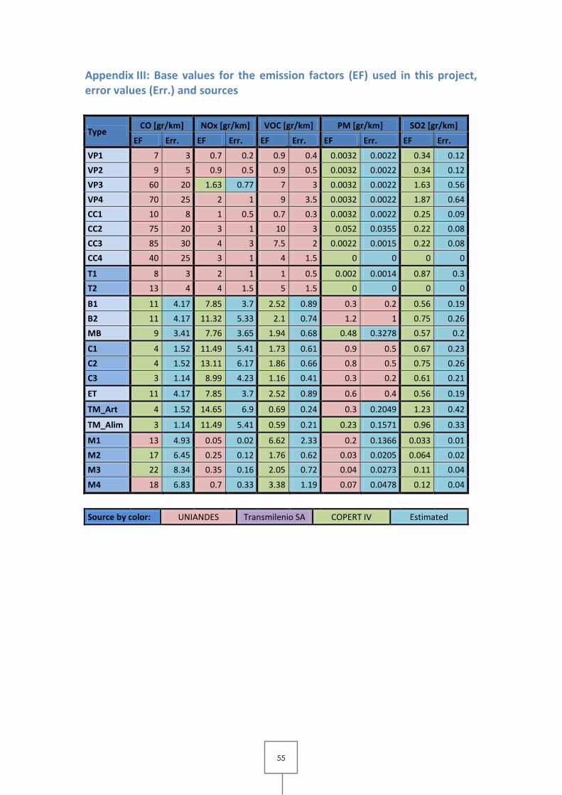
55
Appendix III: Base values for the emission factors (EF) used in this project, error values (Err.) and sources
Type CO [gr/km] NOx [gr/km] VOC [gr/km] PM [gr/km] SO2 [gr/km]
EF Err. EF Err. EF Err. EF Err. EF Err.
VP1 7 3 0.7 0.2 0.9 0.4 0.0032 0.0022 0.34 0.12
VP2 9 5 0.9 0.5 0.9 0.5 0.0032 0.0022 0.34 0.12
VP3 60 20 1.63 0.77 7 3 0.0032 0.0022 1.63 0.56
VP4 70 25 2 1 9 3.5 0.0032 0.0022 1.87 0.64
CC1 10 8 1 0.5 0.7 0.3 0.0032 0.0022 0.25 0.09
CC2 75 20 3 1 10 3 0.052 0.0355 0.22 0.08
CC3 85 30 4 3 7.5 2 0.0022 0.0015 0.22 0.08
CC4 40 25 3 1 4 1.5 0 0 0 0
T1 8 3 2 1 1 0.5 0.002 0.0014 0.87 0.3
T2 13 4 4 1.5 5 1.5 0 0 0 0
B1 11 4.17 7.85 3.7 2.52 0.89 0.3 0.2 0.56 0.19
B2 11 4.17 11.32 5.33 2.1 0.74 1.2 1 0.75 0.26
MB 9 3.41 7.76 3.65 1.94 0.68 0.48 0.3278 0.57 0.2
C1 4 1.52 11.49 5.41 1.73 0.61 0.9 0.5 0.67 0.23
C2 4 1.52 13.11 6.17 1.86 0.66 0.8 0.5 0.75 0.26
C3 3 1.14 8.99 4.23 1.16 0.41 0.3 0.2 0.61 0.21
ET 11 4.17 7.85 3.7 2.52 0.89 0.6 0.4 0.56 0.19
TM_Art 4 1.52 14.65 6.9 0.69 0.24 0.3 0.2049 1.23 0.42
TM_Alim 3 1.14 11.49 5.41 0.59 0.21 0.23 0.1571 0.96 0.33
M1 13 4.93 0.05 0.02 6.62 2.33 0.2 0.1366 0.033 0.01
M2 17 6.45 0.25 0.12 1.76 0.62 0.03 0.0205 0.064 0.02
M3 22 8.34 0.35 0.16 2.05 0.72 0.04 0.0273 0.11 0.04
M4 18 6.83 0.7 0.33 3.38 1.19 0.07 0.0478 0.12 0.04
Source by color: UNIANDES Transmilenio SA COPERT IV Estimated

56
Appendix IV: Mobile sources emission factors for the different pollutants, each vehicle category and each road category of the first modeling attempt
Emission factors NOX [g/km*veh]
NOx PRINC SEC RUR TM_Art TM_Alim
VP+CC 1.84 1.48 2.15 1.68 1.61
T 3.35 3.22 3.75 3.25 3.25
B+MB 8.83 8.80 9.23 8.78 8.76
C 10.65 10.55 11.05 10.54 10.55
ET 7.90 7.90 8.30 7.85 7.80
TM-Art 14.70 14.70 15.10 14.65 14.60
TM-Alim 11.60 11.50 12.00 11.49 11.50
M 0.25 0.19 0.35 0.22 0.21
Vel [km/h] 35 20 60 27 13
Emission factors CO [g/km*veh]
CO PRINC SEC RUR TM_Art TM_Alim
VP+CC 36.15 50.13 30.62 40.60 44.38
T 8.32 19.18 4.81 11.14 13.48
B+MB 8.50 13.45 6.20 10.39 11.60
C 2.63 5.09 1.95 3.45 3.99
ET 7.60 11.50 6.20 11.00 10.00
TM-Art 2.90 5.80 2.00 4.00 4.70
TM-Alim 2.40 4.50 1.90 3.00 3.40
M 13.39 22.49 13.98 16.42 18.64
Vel [km/h] 35 20 60 27 13
Emission factors SO2 [g/km*veh]
SO2 PRINC SEC RUR TM_Art TM_Alim
VP+CC 0.80 0.80 0.80 0.80 0.80
T 0.32 0.32 0.32 0.32 0.32
B+MB 0.62 0.62 0.62 0.62 0.62
C 0.66 0.66 0.66 0.66 0.66
ET 0.56 0.56 0.56 0.56 0.56
TM-Art 1.23 1.23 1.23 1.23 1.23
TM-Alim 0.96 0.96 0.96 0.96 0.96
M 0.06 0.06 0.06 0.06 0.06
Vel [km/h] 35 20 60 27 13

57
Emission factors VOCs [g/km*veh]
VOCs PRINC SEC RUR TM_Art TM_Alim
VP+CC 4.45 6.76 3.70 5.07 5.50
T 2.31 3.72 1.75 2.73 3.00
B+MB 1.37 2.75 0.82 1.72 2.01
C 2.10 3.65 1.32 2.62 2.98
ET 2.00 4.00 1.10 2.52 3.00
TM-Art 0.59 0.80 0.40 0.69 0.75
TM-Alim 0.10 0.15 0.06 0.12 0.14
M 5.22 4.41 5.21 4.94 4.78
Vel [km/h] 35 20 60 27 13
Emission factors PM [g/km*veh]
PM PRINC SEC RUR TM_Art TM_Alim
VP+CC 0.01 0.01 0.00 0.01 0.01
T 0.00 0.00 0.00 0.00 0.00
B+MB 0.44 0.54 0.39 0.44 0.49
C 0.50 0.64 0.43 0.50 0.56
ET 0.55 0.41 0.20 0.55 0.63
TM-Art 0.25 0.38 0.17 0.25 0.33
TM-Alim 0.18 0.31 0.10 0.18 0.26
M 0.07 0.07 0.07 0.07 0.07
Vel [km/h] 35 20 60 27 13

58
Appendix V: Proportioned flux data as used for the distribution in time in the first application of the model
Hour VP_CC T BMB C ET M TM
1 0.0116 0.0116 0.0024 0.0124 0.0047 0.0060 0.0130
2 0.0080 0.0080 0.0008 0.0137 0.0031 0.0033 0.0130
3 0.0065 0.0065 0.0006 0.0110 0.0022 0.0030 0.0325
4 0.0065 0.0065 0.0013 0.0162 0.0029 0.0029 0.0325
5 0.0101 0.0101 0.0092 0.0263 0.0171 0.0060 0.0455
6 0.0272 0.0272 0.0408 0.0420 0.0562 0.0269 0.0584
7 0.0477 0.0477 0.0633 0.0482 0.0804 0.0643 0.0584
8 0.0595 0.0595 0.0654 0.0428 0.0709 0.0811 0.0584
9 0.0544 0.0544 0.0644 0.0495 0.0654 0.0640 0.0584
10 0.0546 0.0546 0.0598 0.0631 0.0535 0.0588 0.0455
11 0.0548 0.0548 0.0552 0.0767 0.0416 0.0536 0.0455
12 0.0552 0.0552 0.0557 0.0699 0.0440 0.0530 0.0455
13 0.0559 0.0559 0.0567 0.0650 0.0492 0.0483 0.0455
14 0.0562 0.0562 0.0564 0.0619 0.0491 0.0502 0.0455
15 0.0603 0.0603 0.0553 0.0653 0.0475 0.0543 0.0455
16 0.0578 0.0578 0.0572 0.0663 0.0559 0.0595 0.0584
17 0.0553 0.0553 0.0592 0.0674 0.0642 0.0647 0.0584
18 0.0584 0.0584 0.0589 0.0567 0.0688 0.0769 0.0584
19 0.0573 0.0573 0.0576 0.0409 0.0633 0.0710 0.0455
20 0.0585 0.0585 0.0525 0.0321 0.0506 0.0476 0.0455
21 0.0499 0.0499 0.0478 0.0272 0.0380 0.0363 0.0325
22 0.0415 0.0415 0.0409 0.0181 0.0328 0.0319 0.0325
23 0.0296 0.0296 0.0279 0.0138 0.0255 0.0247 0.0130
24 0.0231 0.0231 0.0109 0.0136 0.0131 0.0120 0.0130

59
Appendix VI: Map of the 20 localities composing the district of Bogotá
(Source: http://sites.google.com/a/civilju.com/www/01_Bogota_Localidades.jpg)

60
Appendix VII: Maximum values for each category in the road survey
Survey Point All Light Bus Truck
KR 10 X CL 19 6876 3906 2117 95
AUTOPISTA NORTE X CL 127 17559 14758 413 747
AV. BOYACÁ X CL 72 11962 8315 1186 732
AV. AMÉRICAS X KR 42B - CL19 8620 6481 819 410
AUTOPISTA SUR X AV 68 8715 5385 765 617
AUTONORTE X CL 170 12262 9899 506 783
KR 7 X CL 85 5528 4506 400 118
AC 6 X KR 24-27 8577 6200 714 353
AV. BOYACÁ X CAI YOMASA 2053 1073 446 301
AV 1 DE MAYO X TV 42 7340 5238 789 395
AK 68 X AC 26 19028 14784 1568 687
CL 26 X KR 92 8633 6556 816 602
AV. BOYACÁ X CL 13 14839 9059 1067 1222
AV. BOYACÁ X AV V.CIO 6093 3196 635 662
KR 13 X CL 53 3391 2488 510 49
KR 91-94 X CL 131 2537 1120 892 86
KR 7 X CL 127 5589 4629 618 190
KR 10 X AV 1 DE MAYO 4587 2270 1350 109
KR 7 X CL 45 5962 4642 781 74
AV. SUBA X CL 100 11032 8914 586 291
AV. A MEJÍA X AV 1 DE MAYO 4520 1919 775 398
KR 15 X CL 100 6912 5538 768 137
AV. V.CIO X AV G. CORTES 4330 1983 991 289
AV. CENTENARIO X AV. CALI 11839 7363 1020 2013
Source: Road survey data provided from the Secretaria Distrital de Movilidad (SDM)

61
Appendix VIII: Results of the road survey data analysis
Survey Point All Light Bus Truck Combined
KR 10 X CL 19 MEDIUM LOW VERY HIGH LOW MEDIUM
AUTOPISTA NORTE X CL 127 VERY HIGH VERY HIGH LOW HIGH HIGH
AV. BOYACÁ X CL 72 HIGH HIGH HIGH HIGH HIGH
AV. AMÉRICAS X KR 42B - CL19 HIGH MEDIUM MEDIUM MEDIUM HIGH
AUTOPISTA SUR X AV 68 HIGH MEDIUM MEDIUM HIGH HIGH
AUTONORTE X CL 170 VERY HIGH HIGH MEDIUM HIGH HIGH
KR 7 X CL 85 MEDIUM MEDIUM LOW LOW MEDIUM
AC 6 X KR 24-27 HIGH MEDIUM MEDIUM LOW MEDIUM
AV. BOYACÁ X CAI YOMASA LOW LOW LOW LOW LOW
AV 1 DE MAYO X TV 42 MEDIUM MEDIUM MEDIUM LOW MEDIUM
AK 68 X AC 26 VERY HIGH VERY HIGH VERY HIGH HIGH VERY HIGH
CL 26 X KR 92 HIGH MEDIUM MEDIUM HIGH HIGH
AV. BOYACÁ X CL 13 VERY HIGH HIGH HIGH VERY HIGH VERY HIGH
AV. BOYACÁ X AV V.CIO MEDIUM LOW MEDIUM HIGH MEDIUM
KR 13 X CL 53 LOW LOW MEDIUM LOW MEDIUM
KR 91-94 X CL 131 LOW LOW MEDIUM LOW MEDIUM
KR 7 X CL 127 MEDIUM MEDIUM MEDIUM LOW MEDIUM
KR 10 X AV 1 DE MAYO MEDIUM LOW HIGH LOW MEDIUM
KR 7 X CL 45 MEDIUM MEDIUM MEDIUM LOW MEDIUM
AV. SUBA X CL 100 HIGH HIGH MEDIUM LOW HIGH
AV. A MEJÍA X AV 1 DE MAYO MEDIUM LOW MEDIUM LOW MEDIUM
KR 15 X CL 100 MEDIUM MEDIUM MEDIUM LOW MEDIUM
AV. V.CIO X AV G. CORTES MEDIUM LOW MEDIUM LOW MEDIUM
AV. CENTENARIO X AV. CALI HIGH MEDIUM HIGH VERY HIGH HIGH
Source: Road survey data provided from the Secretaria Distrital de Movilidad (SDM)

62
Appendix IX: Illustration of the Thiessen algorithm
The Thiessen algorithm defines areas of influence around each of a set of points using
the perpendicular bisectors of the lines between all the points (ET Geo Wizards, 2010).
All the points of a given set of points are connected by straight lines. These lines are
then divided in halves using the perpendicular bisectors. The zones delimited by the
bisectors are the influence zones for each point. Any location in a given zone is closer
to the point at the center of this zone than to any other point of the set. The concept
is illustrated in Figure 21.
Figure 21: grey lines connect all the points of an input dataset, red lines define the boundaries
of the polygons using a Thiessen method (source: www.ems-i.com)

63
Appendix X: Mobile sources emission factors for the different pollutants, each vehicle category and each road category of the second modeling attempt
Emission factors CO [g/km*veh]
CO PRINC_B PRINC_M PRINC_A PRINC_MA SEC_B SEC_M SEC_A RUR TM_Art TM_Alim
VP_CC 40.60 40.60 40.60 40.60 50.13 50.13 50.13 33.38 0.00 0.00
T 11.14 11.14 11.14 11.14 19.18 19.18 19.18 6.57 0.00 0.00
B_MB 13.45 13.45 13.45 13.45 11.60 11.60 11.60 8.50 0.00 0.00
C 5.09 5.09 5.09 5.09 3.99 3.99 3.99 2.63 0.00 0.00
ET 11.00 11.00 11.00 11.00 11.50 11.50 11.50 6.90 0.00 0.00
TM-Art 0.00 0.00 0.00 0.00 0.00 0.00 0.00 0.00 4.35 0.00
TM-Alim 0.00 0.00 0.00 0.00 0.00 0.00 0.00 0.00 0.00 3.40
M 16.42 16.42 16.42 16.42 22.49 22.49 22.49 13.68 0.00 0.00
Emission factors NOx [g/km*veh]
NOx PRINC_B PRINC_M PRINC_A PRINC_MA SEC_B SEC_M SEC_A RUR TM_Art TM_Alim
VP_CC 1.68 1.68 1.68 1.68 1.48 1.48 1.48 2.00 0.00 0.00
T 3.25 3.25 3.25 3.25 3.22 3.22 3.22 3.55 0.00 0.00
B_MB 8.80 8.80 8.80 8.80 8.76 8.76 8.76 8.83 0.00 0.00
C 10.55 10.55 10.55 10.55 10.55 10.55 10.55 10.65 0.00 0.00
ET 7.85 7.85 7.85 7.85 7.90 7.90 7.90 8.10 0.00 0.00
TM-Art 0.00 0.00 0.00 0.00 0.00 0.00 0.00 0.00 14.70 0.00
TM-Alim 0.00 0.00 0.00 0.00 0.00 0.00 0.00 0.00 0.00 11.50
M 0.22 0.22 0.22 0.22 0.19 0.19 0.19 0.30 0.00 0.00
Emission factors PM [g/km*veh]
PM PRINC_B PRINC_M PRINC_A PRINC_MA SEC_B SEC_M SEC_A RUR TM_Art TM_Alim
VP_CC 0.01 0.01 0.01 0.01 0.01 0.01 0.01 0.01 0.00 0.00
T 0.00 0.00 0.00 0.00 0.00 0.00 0.00 0.00 0.00 0.00
B_MB 0.54 0.54 0.54 0.54 0.49 0.49 0.49 0.44 0.00 0.00
C 0.64 0.64 0.64 0.64 0.56 0.56 0.56 0.50 0.00 0.00
ET 0.55 0.55 0.55 0.55 0.41 0.41 0.41 0.38 0.00 0.00
TM-Art 0.00 0.00 0.00 0.00 0.00 0.00 0.00 0.00 0.32 0.00
TM-Alim 0.00 0.00 0.00 0.00 0.00 0.00 0.00 0.00 0.00 0.26
M 0.07 0.07 0.07 0.07 0.07 0.07 0.07 0.07 0.00 0.00

64
Emission factors SO2 [g/km*veh]
SO2 PRINC_B PRINC_M PRINC_A PRINC_MA SEC_B SEC_M SEC_A RUR TM_Art TM_Alim
VP_CC 0.80 0.80 0.80 0.80 0.80 0.80 0.80 0.80 0.00 0.00
T 0.32 0.32 0.32 0.32 0.32 0.32 0.32 0.32 0.00 0.00
B_MB 0.62 0.62 0.62 0.62 0.62 0.62 0.62 0.62 0.00 0.00
C 0.66 0.66 0.66 0.66 0.66 0.66 0.66 0.66 0.00 0.00
ET 0.56 0.56 0.56 0.56 0.56 0.56 0.56 0.56 0.00 0.00
TM-Art 0.00 0.00 0.00 0.00 0.00 0.00 0.00 0.00 1.23 0.00
TM-Alim 0.00 0.00 0.00 0.00 0.00 0.00 0.00 0.00 0.00 0.96
M 0.06 0.06 0.06 0.06 0.06 0.06 0.06 0.06 0.00 0.00
Emission factors VOCs [g/km*veh]
VOCs PRINC_B PRINC_M PRINC_A PRINC_MA SEC_B SEC_M SEC_A RUR TM_Art TM_Alim
VP_CC 5.07 5.07 5.07 5.07 6.76 6.76 6.76 4.07 0.00 0.00
T 2.73 2.73 2.73 2.73 3.72 3.72 3.72 2.03 0.00 0.00
B_MB 2.75 2.75 2.75 2.75 2.01 2.01 2.01 1.37 0.00 0.00
C 3.65 3.65 3.65 3.65 2.98 2.98 2.98 2.10 0.00 0.00
ET 2.52 2.52 2.52 2.52 4.00 4.00 4.00 1.55 0.00 0.00
TM-Art 0.00 0.00 0.00 0.00 0.00 0.00 0.00 0.00 0.70 0.00
TM-Alim 0.00 0.00 0.00 0.00 0.00 0.00 0.00 0.00 0.00 0.14
M 4.94 4.94 4.94 4.94 4.41 4.41 4.41 5.22 0.00 0.00

65
Appendix XI: Graphical analysis of the traffic distribution in time on the different main road subcategories
Traffic charge evolution in time, as fraction of daily traffic: Low traffic
Traffic charge evolution in time, as fraction of daily traffic: Medium traffic
0
0.01
0.02
0.03
0.04
0.05
0.06
0.07
0.08
0.09
0.1
1 6 11 16 21
Fra
ctio
n o
f d
ail
y t
raff
ic [
-]
Time of the day [h]
VP+CC
T
B+MB
C
ET
M
0
0.01
0.02
0.03
0.04
0.05
0.06
0.07
0.08
0.09
1 6 11 16 21
Fra
ctio
n o
f d
ail
y t
raff
ic [
-]
Time of the day [h]
VP+CC
T
B+MB
C
ET
M

66
Traffic charge evolution in time, as fraction of daily traffic: High traffic
Traffic charge evolution in time, as fraction of daily traffic: Very high traffic
0
0.01
0.02
0.03
0.04
0.05
0.06
0.07
0.08
0.09
0.1
1 6 11 16 21
Fra
ctio
n o
f d
ail
y t
raff
ic [
-]
Time of the day [h]
VP+CC
T
B+MB
C
ET
M
0
0.02
0.04
0.06
0.08
0.1
0.12
1 6 11 16 21
Fra
ctio
n o
f d
ail
y t
raff
ic [
-]
Time of the day [h]
VP+CC
T
B+MB
C
ET
M

67
Appendix XII: Classification Diagram for the Industrial Categories in Bogotá based on their technology and size, adapted from (CIIA, 2008a)
Type of source Characteristics Fuel used Category
> 100 BHP and build < 1997 Natural Gas CG1
> 100 BHP Coal CC1
Boiler > 100 BHP and build > 1997 Natural Gas CG2
Natural Gas CG3
< 100 BHP
Coal CC2
Food production Natural Gas HG1
Drying and Natural Gas HG2
Oven
Oven Coal HC
Brick burning kiln Coal HL
GPL GPL
Boiler Diesel D
Used Veg. Oil AU

68
Appendix XIII: Graphical representation of the hourly industrial sources emissions for the pollutants considered in this project
0
10000
20000
30000
40000
50000
60000
70000
80000
90000
1 3 5 7 9 11 13 15 17 19 21 23
Em
isio
ne
s [g
r/h
]
Hora [h]
Emisiones de CO
0
50000
100000
150000
200000
250000
300000
350000
1 3 5 7 9 11 13 15 17 19 21 23
Em
isio
ne
s [g
/h
]
Hora [h]
Emisiones de NOx

69
0
50000
100000
150000
200000
250000
300000
350000
1 3 5 7 9 11 13 15 17 19 21 23
Em
isio
ne
s [g
/h
]
Hora [h]
Emisiones de SO2
0
20000
40000
60000
80000
100000
120000
140000
160000
180000
1 3 5 7 9 11 13 15 17 19 21 23
Em
isio
ne
s [g
/h
]
Hora [h]
Emisiones de PM

70
Appendix XIV: SO2 emissions from mobile sources at 08h00, based on the second application of the model