
An Electro- Magneto-Static Field for Confinement of .../67531/metadc500001/m2/1/high... · CHARGED...
116
APPROVED: Ducan L. Weathers, Major Professor Carlos A. Ordonez, Co-Major Professor Floyd D. McDaniel, Committee Member Tilo Reinert, Committee Member Chris Littler, Chair of the Department of Physics Mark Wardell, Dean of the Toulouse Graduate School AN ELECTRO- MAGNETO-STATIC FIELD FOR CONFINEMENT OF CHARGED PARTICLE BEAMS AND PLASMAS Josè L. Pacheco Dissertation Prepared for the Degree of DOCTOR OF PHILOSOPHY UNIVERSITY OF NORTH TEXAS May 2014
Transcript of An Electro- Magneto-Static Field for Confinement of .../67531/metadc500001/m2/1/high... · CHARGED...

APPROVED: Ducan L. Weathers, Major Professor Carlos A. Ordonez, Co-Major Professor Floyd D. McDaniel, Committee Member Tilo Reinert, Committee Member Chris Littler, Chair of the Department
of Physics Mark Wardell, Dean of the Toulouse
Graduate School
AN ELECTRO- MAGNETO-STATIC FIELD FOR CONFINEMENT OF
CHARGED PARTICLE BEAMS AND PLASMAS
Josè L. Pacheco
Dissertation Prepared for the Degree of
DOCTOR OF PHILOSOPHY
UNIVERSITY OF NORTH TEXAS
May 2014

Pacheco, Josè L. An Electro- Magneto-Static Field for Confinement of Charged
Particle Beams and Plasmas. Doctor of Philosophy (Physics), May 2014, 101 pp., 34
figures, 40 numbered references.
A system is presented that is capable of confining an ion beam or plasma within
a region that is essentially free of applied fields. An Artificially Structured Boundary
(ASB) produces a spatially periodic set of magnetic field cusps that provides charged
particle confinement. Electrostatic plugging of the magnetic field cusps enhances
confinement. An ASB that has a small spatial period, compared to the dimensions of a
confined plasma, generates electro- magneto-static fields with a short range. An ASB-
lined volume thus constructed creates an effectively field free region near its center. It is
assumed that a non-neutral plasma confined within such a volume relaxes to a Maxwell-
Boltzmann distribution. Space charge based confinement of a second species of charged
particles is envisioned, where the second species is confined by the space charge of the
first non-neutral plasma species. An electron plasma confined within an ASB-lined
volume can potentially provide confinement of a positive ion beam or positive ion
plasma.
Experimental as well as computational results are presented in which a plasma or
charged particle beam interact with the electro- magneto-static fields generated by an
ASB. A theoretical model is analyzed and solved via self-consistent computational
methods to determine the behavior and equilibrium conditions of a relaxed plasma. The
equilibrium conditions of a relaxed two species plasma are also computed. In such a
scenario, space charge based electrostatic confinement is predicted to occur where a
second plasma species is confined by the space charge of the first plasma species. An

experimental apparatus with cylindrical symmetry that has its interior surface lined
with an ASB is presented. This system was developed by using a simulation of the
electro- magneto-static fields present within the trap to guide mechanical design. The
construction of the full experimental apparatus is discussed. Experimental results that
show the characteristics of electron beam transmission through the experimental
apparatus are presented. A description of the experimental hardware and software used
for trapping a charged particle beam or plasma is also presented.

ii
Copyright 2014
by
Josè L. Pacheco

iii
ACKNOWLEDGEMENTS
This work is dedicated to Nataly for her unconditional love, support, and patience! and
to my Mother and Father.†
I would like to thank Naresh T. Deoli and Allen S. Kiester for their help,
suggestions, and friendship; Kurt Weihe, Paul Jones, and Gary Karnes for assisting with
technical support; the Ion Beam Modification and Analysis Lab (IBMAL) for supplying
the necessary experimental equipment; and UNT's High Performance Computing
Initiative for providing computational resources.
The material presented is based upon work supported by the Department of
Energy under Grant No. DE-FG02-06ER54883 and by the National Science Foundation
under Grant No. PHY-1202428. The research that appears in this dissertation is, in
part, a compilation of published work:
• “Plasma Interaction With a Static Spatially Periodic Electromagnetic Field,” J. L. Pacheco, C. A. Ordonez, and D. L. Weathers. IEEE Transactions on Plasma Science, Vol. 39, no. 11, pp. 2424-2425, Nov. 2011 doi: 10.1109/TPS.2011.2158669.
• “Spatially Periodic Electromagnetic Force Field For Plasma Confinement and Control,” C. A. Ordonez, J. L. Pacheco, and D. L. Weathers. The Open Plasma Physics Journal, 5(2012). pp. 1-10. doi: 10.2174/1876534301205010001. (Section VI)
• “Artificially Structured Boundary for a High Purity Ion Trap or Ion Source,” J. L. Pacheco, C. A. Ordonez, and D. L. Weathers. Nucl. Instr. and Meth. in Phys. Res. B. Conf. Proc. 21st International Conference on Ion Beam Analysis. Seattle, WA. 2013.
• “Space-charge-based electrostatic plasma confinement involving relaxed plasma species,” J. L. Pacheco, C. A. Ordonez, and D. L. Weathers. Physics of Plasmas, 19, 102510 (2012), DOI: http://dx.doi.org/10.1063/1.4764076.
• “Electrostatic Storage Ring With Focusing Provided By the Space Charge of an Electron Plasma,” J. L. Pacheco, C. A. Ordonez, and D. L. Weathers. Application of Accelerators in Research and Industry, AIP Conference Proceedings 1525 (2013) 88-93.

iv
TABLE OF CONTENTS
Page ACKNOWLEDGEMENTS ............................................................................................ iii LIST OF FIGURES ....................................................................................................... vi CHAPTER 1. INTRODUCTION .................................................................................... 1 CHAPTER 2. PLASMA INTERACTION WITH A STATIC SPATIALLY PERIODIC ELECTROMAGNETIC FIELD ...................................................................................... 4
2.1. Introduction ............................................................................................... 4 2.2. Experiment: A Proof of Concept ................................................................ 6 2.3. Results ....................................................................................................... 9
CHAPTER 3. ARTIFICIALLY STRUCTURED BOUNDARY FOR A HIGH PURITY ION TRAP OR ION SOURCE ...................................................................................... 11
3.1. Introduction .............................................................................................. 11 3.2. Theory ...................................................................................................... 12 3.3. Results ...................................................................................................... 17 3.4. Conclusion ................................................................................................. 22
CHAPTER 4. SPACE-CHARGE-BASED ELECTROSTATIC PLASMA CONFINEMENT INVOLVING RELAXED PLASMA SPECIES ................................. 23
4.1. Introduction .............................................................................................. 23 4.2. Single-Species Non-Neutral Plasma ........................................................... 25 4.3. Two-Species Plasma .................................................................................. 31 4.4. Space-Charge-Based Electrostatic Confinement Conditions ...................... 35 4.5. Conclusion ................................................................................................. 38
CHAPTER 5. ELECTROSTATIC STORAGE RING WITH FOCUSING PROVIDED BY THE SPACE CHARGE OF AN ELECTRON PLASMA ........................................ 42
5.1. Introduction .............................................................................................. 42 5.2. Theory ...................................................................................................... 43 5.3. Results ...................................................................................................... 46 5.4. Space-Charge-Based Electrostatic Focusing .............................................. 51 5.5. Conclusion ................................................................................................. 53

v
CHAPTER 6. ELECTRON BEAM TRANSMISSION THROUGH A CYLINDRICALLY SYMMETRIC ARTIFICIALLY STRUCTURED BOUNDARY .... 55
6.1. Introduction .............................................................................................. 55 6.2. Apparatus ................................................................................................. 55 6.3. Electron Beam .......................................................................................... 56 6.4. Experimental Artificially Structured Boundary ........................................ 58 6.5. UHV Conditions During Experimentation ................................................ 61 6.6. Electron Detection System ........................................................................ 62 6.7. Accepance and Transmission Without Electrostatic Plugging .................. 63 6.8. Summary and Conclusion ......................................................................... 69
CHAPTER 7. CONCLUSION ........................................................................................ 70 APPENDIX A. NORMALIZATION OF MAXWELLIAN DISTRIBUTION ................ 72 APPENDIX B. PRODUCT LOGARITHM ................................................................... 75 APPENDIX C. TRAPPING FIELDS, PARTICLE BEHAVIOR, AND PLASMA BEHAVIOR ................................................................................................................... 82 APPENDIX D. CHARGED PARTICLE TRAPPING .................................................. 88 BIBLIOGRAPHY ........................................................................................................... 97

LIST OF FIGURES
2.1 Nested Penning trap. Rectangular segments are the locations of posi-
tively (red) and negatively (blue) biased electrodes. The center electrode
is typically grounded. A positively charged particle (red oval region) is
confined between the positively biased electrodes. A negatively charged
particle (blue oval region) is confined between the outer-most set of elec-
trodes. The magnetic field keeps particles with either sign of charge
radially confined.......................................................................................... 5
2.2 A section of a planar ASB: Four permanent magnets with electrostatic
plugging applied using copper electrodes (left). Corresponding simula-
tion of the magnetic field lines for magnets with a maximum magnetic
field magnitude Bmax = 1 T, and like poles facing each other (right). The
fields of interest lie in the two quadrants on the right. A typical magnetic
field cusp is present near the center of the figure, at the intersection of
the axes. ...................................................................................................... 6
2.3 Conceptual experimental setup as used to observe plasma interaction
with an ASB. See text for description of experiment.................................. 7
2.4 Left: Argon ions incident on magnet structure with electrostatic plugging
turned off (electrodes, magnets, and supporting structure are at ground
potential). Right: Electrostatic plugging turned on (reflection electrodes
at 30 V). Positively charged particles enter magnetic cusps in both left
and right panels. In the right panel, particles that enter a cusp experience
an E ×B drift that guides them into, or out of, the plane of the page,
thereby extending the plasma perpendicular to the plane of the page.
The brightness is enhanced where the E ×B drifts occur. ...................... 8
vi

2.5 Electrons incident on magnet structure. Left: Electrostatic plugging
turned off. Right: Electrostatic plugging turned on (−200 V). Right:
The E × B drift caused the plasma to reach and pass in front of the
ends of the magnets closest to the camera. ................................................. 9
3.1 Simulation environment representing two periods of a planar ASB. Ions
are confined to the region below the ASB (yn < 0). The lower edge of
the ASB is located at yn = 0. The dots mark the positions of the current
carrying wires, with current that alternates in sign from one column
of wires to the next, ±I. Magnetic field cusps are produced with the
direction of the magnetic field labeled by βt. The electrodes are marked
by lines, which represent their lengths and locations in the simulation
environment. The current carrying wires and the electrodes are infinite
in extent in the z dimension. The electrostatic potential energy barrier
is located in the region 0.5 ≤ yn ≤ 0.75, at the location of V1. V0 and V2
are at ground potential. φ0 is the electric potential at the center of the
anode gap, where the magnetic field has a magnitude B0. See Eq. (2)
for details regarding ηi, and ∆yn. ............................................................... 14
3.2 Simulation that represents a two period segment of an ASB. The differ-
ent shades show trajectories with φn0 = 1 and δ = 1000 (black), δ =
100 (dark gray), and δ = 20 (light gray). The trajectory calculation is
terminated when a particle reaches yn = 0.75............................................. 18
3.3 Simulation that represents a two period segment of an ASB. The different
shades show trajectories with δ = 20, and φn0 = 0.5 (light gray) and
φn0 = 5 (black). The trajectory calculation is terminated when a particle
reaches yn = 0.75......................................................................................... 19
vii

3.4 Profile of the spatial distribution of charged particles that reached yn ≥0.75 after entering a cusp and overcoming the electrostatic potential bar-
rier. The distribution of particles at yn ≈ 0.75 is for φn0 = 1 and δ =
10, 20, and 40. The data series are labeled according to the parame-
ter varied, and the corresponding percentages of particles that reached
yn ≈ 0.75 are indicated. The total number of trajectories simulated for
each of these plots was 100,000. .................................................................. 20
3.5 Profile of the spatial distribution of charged particles that reached yn ≥0.75 after entering a cusp and overcoming the electrostatic potential bar-
rier. The distribution is for δ = 20 and φn0 = 0.5, 1, and 2. The data
series are labeled according to the parameter varied, and the correspond-
ing percentages of particles that reached yn ≈ 0.75 are indicated. The
total number of trajectories simulated for each of these plots was 100,000. 21
4.1 Conceptual model of a plasma trapping volume with a field free region
at its center. A plasma is envisioned to relax within the volume and be
“edge-confined” by a reflecting surface such as an ASB. ............................ 24
4.2 Typical radial profile of the normalized electrostatic potential. The plots
are for rn,max = 100 and α = 1 (solid), 2 (long dash), 3 (short dash).
The normalized electrostatic potential difference between the center and
the boundary is 7.6 for α = 1, 7.2 for α = 2, and 6.8 for α = 3.................. 29
4.3 Typical normalized density profiles. The plots are for α = 3 and rn,max =
5 (dot-dashed), 10 (short dash), 20 (long dash), 30 (solid). Similar pro-
files occur for other values of α. ................................................................ 29
4.4 Normalized electrostatic potential difference (between plasma center and
edge) for the three geometries. The solid lines are Eq. (26). ...................... 30
viii

4.5 Normalized electrostatic potential of a two-species plasma (top). Self-
consistent distributions of the two plasma species (bottom) in logarithmic
scale. The plots are for, Tn = 5, rn,max = 30, and Nn = 0.004 (dashed),
0.04 (dot-dashed), 0.4 (solid). The arrows indicate the trend that the
system follows as Nn is increased. In the lower panel of this figure and
Figs. 4.6-4.8, the normalized distributions are n−(rn)/n0− , which are la-
beled by minus signs (–), and Zn+(rn)/n0− , which are labeled by plus
signs (+). Thus, each matching pair of plots are the normalized distri-
butions for the negative and positive plasma species. ................................. 33
4.6 Normalized electrostatic potential of a two-species plasma (top). Self-
consistent distributions of the two plasma species (bottom). The plots
are for Nn = 0.02, rn,max = 30, and Tn = 1 (solid), 15 (dot-dashed), and
30 (dashed). The ± labels are defined in Fig. 4.5....................................... 34
4.7 Two plasma species with equal temperatures and charge states. The
plots are for Tn = 1, rn,max = 30, and Nn = 0.1 (dot-dashed), 0.01
(dashed), and 0.001 (solid). The ± labels are defined in Fig. 4.5. .............. 36
4.8 Two plasma species with approximately equal charge densities at the
center of the plasma system. The plots are for rn,max = 30 and (Tn, Nn) =
(1, 0.05)[solid], (10, 0.0225)[dot-dashed], (25, 0.0152)[long dash], and (40,
0.0145)[short dash]. The normalized electron temperatures, Tn, were
chosen and the normalized positive plasma charge densities, Nn, were
then adjusted to the lowest value at which the two distributions have
approximately the same value at the center of the system. The ± labels
are defined in Fig. 4.5. ................................................................................ 37
ix

4.9 Normalized electrostatic potential energy well depth for space-charge-
based electrostatic plasma confinement as a function of normalized sys-
tem size. The dotted line in the top panel is for Nn = 0 and Tn = 1.
Top (bottom) panel is for Tn = 1 (Tn = 10), and Nn = 0.1 (solid), 0.01
(long dash), 0.001 (dash), 0.0001 (dot-dashed). .......................................... 39
4.10 Normalized electrostatic potential difference for increasing normalized
charge density of the positive species. There are plot points for rn,max =
300 and Tn = 1, 4, and 10, for each value of Nn, but the plot points are
indistinguishable. The solid line is Eq. (34)................................................ 40
5.1 Cross-sections of a segment of a cylindrical beam line. The electron
plasma is confined by an artificially structured boundary. The space
charge of the electron plasma creates an electrostatic potential that fo-
cuses a positive-ion beam or drifting plasma. ............................................. 44
5.2 Normalized electrostatic potential of a two-species system (top). Self-
consistent distributions of the two species (bottom) in logarithmic scale.
The plots are for, Tn = 5, rn,max = 30, and Nn = 0.004 (dashed), 0.04
(dot-dashed), 0.4 (solid). The arrows indicate the trend that the system
follows as Nn is increased. In the lower panel of this figure and Figs. 5.3-
5.5, the normalized distributions are n−(rn)/n0− , which are labeled by
minus signs (–), and Zn+(rn)/n0− , which are labeled by plus signs (+).
Thus, each matching pair of plots are the normalized distributions for
the negative and positive plasma species. ................................................... 47
5.3 Normalized electrostatic potential of a two-species plasma (top). Self-
consistent distributions of the two plasma species (bottom). The plots
are for Nn = 0.02, rn,max = 30, and Tn = 1 (solid), 15 (dot-dashed), and
30 (dashed). The ± labels are defined in Fig. 5.2....................................... 48
x

5.4 Two plasma species with equal temperatures and charge states. The
plots are for Tn = 1, rn,max = 30, and Nn = 0.1 (dot-dashed), 0.01
(dashed), and 0.001 (solid). The ± labels are defined in Fig. 5.2. .............. 49
5.5 Two plasma species with approximately equal charge densities at the cen-
ter of the plasma system. The plots are for rn,max = 30 and (Tn, Nn) =
(1, 0.05)[solid], (10, 0.0225)[dot-dashed], (25, 0.0152)[long dash], and
(40, 0.0145)[short dash]. The normalized electron temperatures Tn were
chosen and the normalized positive plasma charge densities Nn were then
adjusted to the lowest value at which the two distributions have approx-
imately the same value at the center of the system. The ± labels are
defined in Fig. 5.2. ...................................................................................... 50
5.6 Normalized electrostatic potential energy well depth for space-charge-
based electrostatic focusing as a function of normalized system size. The
plots are for Tn = 1, and Nn = 0 (dotted), 0.0001 (dot-dashed), 0.001
(dash), 0.01 (long dash), and 0.1 (solid). .................................................... 51
5.7 Normalized electrostatic potential difference for increasing normalized
charge density of the positive species. Points are plotted for rn,max =
300 and Tn = 1, 4, and 10, for each value of Nn, but these plot are
indistinguishable for the different values of Tn. The solid line drawn
through the points is a fit given by Eq. (47)............................................... 52
6.1 Schematic view of experimental apparatus. ................................................ 56
xi

6.2 Relative number of particles incident at the entrance of the trap as a
function of the magnitude of einzel lens focusing voltage. The einzel
lens was biased to provide focusing in decelerating mode. 5,000 electron
trajectories were simulated per data point marked by a cross. The maxi-
mum number of electron trajectories that collapsed onto the Faraday cup
electrode was 3472, occurring at an einzel bias voltage of −24 V. Data
points marked by dots are the electron currents observed at the Faraday
cup in the experimental setup, normalized to the maximum current of
−63.5 nA observed for an einzel lens bias of −24 V. ................................... 58
6.3 A length-wise cross-sectional view of the cylindrically symmetric ASB
and the fields produced within its interior. The rectangular features on
the top and bottom figures are the magnets and electrodes that create
the ASB. The lines in the top figure show contours of equal electric
potential. The lines on the bottom figure show the magnetic field. See
text for further details................................................................................. 59
6.4 Photographs of the experimental system. Panel A shows the alternating
sequence of copper ring electrodes and permanent ring magnets. Panel B
shows the trapping volume as viewed upstream from the exit side. Panel
C shows the phosphor screen that, along with the micro-channel plates
(not shown), constitute the electron detection system................................ 60
6.5 Phosphor screen as imaged by SBIG ST-7XMEI SBIG CCD camera
(left panel). An electron beam exiting the trap and incident on the
MCP/Phosphor assembly creates the time integrated fluorescence recorded
by the CCD camera (right panel). For reference, the phosphor screen
(major circular feature on left panel) is 1.9 cm in diameter (or≈ 500 pixels;
1 pixel unit (pu) = 38µm). The same scale applies to right panel............. 62
xii

6.6 Electron beam acceptance into the trap as a function of einzel lens volt-
age. Data points marked by dots are the normalized charge collected
on the unbiased plugging electrodes. Data points marked by crosses
are the time and space integrated relative beam intensities obtained by
processing the images recorded with the CCD camera. See text for details. 64
6.7 Spatial electron beam profile distribution as a function of focusing at the
entrance to the trap. The three dimensional shape that protrudes from
the x-y plane in the z direction is a plot of intensity I(in arbitrary units
(au)) as a function of position. The bands represent equal fractional
intervals of the peak intensity in each of the panels. A contour plot is
also shown at the top of each figure to illustrate the 2D beam profile. The
data processed for the plots shown are the pixel values that represent the
images of the beam as captured from the phosphor screen by the CCD
camera. An example of such an image is shown in the right panel of
Fig. 6.5. The x and y coordinates are in pixel size units (pu). ................... 65
xiii

CHAPTER 1
INTRODUCTION
The current project emerged from a quest for alternative ways to simultaneously
confine and control charged particles of either sign of charge. Confinement of both signs
of charge in overlapping volumes presents an ideal environment for experimentation with
non-neutral plasmas, partially neutralized plasmas, charged particles, and charged-particle
beams. Applications of such a system include the confinement of a two-species plasma for
recombination studies, lining of plasma facing components to minimize unwanted erosion,
guiding of neutral and partially neutralized ion beams, confinement of non-neutral or par-
tially neutralized non-drifting plasmas, ion accumulators, high purity ion sources, and for
experiments in atomic and molecular physics.
In the trapping system presented here, the reflection of charged particle trajectories
occurs near the confining boundary, where the confining fields have a relatively high strength.
Away from the boundary, an essentially field free region exists, where confined particles are
expected to reside. A field-free confinement region is highly desired as a prospecting tool
for experiments with particle trapping, particle-particle interaction, particle-external field
interaction, and self-consistent relaxation of plasmas. It is envisioned that the concept
described herein could be employed in conjunction with, or as an alternative to, systems
that currently exist for charged particle, or plasma, confinement and control.
In Chapter 2, initial research on an electro- magneto-static field for reflection and
confinement of charged particles is presented. The structure consists of an artificially struc-
tured boundary (ASB) with electrostatic plugging applied. An ASB generates a spatially
periodic sequence of magnetic field cusps. Electrostatic plugging occurs with applied poten-
tial variations along the magnetic field cusps that are similar to those applied to one side of
a nested Penning trap. A field thus created allows for the simultaneous reflection of charged
particles of either sign of charge that are incident randomly. Experimental results that show
the behavior of an argon plasma and an electron plasma are reported.
1

In Chapter 3, a plasma enclosed by an artificially structured boundary (ASB) is
proposed as an alternative to existing ion source assemblies. In accelerator applications,
many ion sources can have a limited lifetime or frequent service intervals due to sputtering
and eventual degradation of the ion source assembly. Ions are accelerated towards the exit
canal of positive ion sources, whereas, due to the biasing scheme, electrons or negative ions are
accelerated towards the back of the ion source assembly. This can either adversely affect the
experiment in progress due to sputtered contamination or compromise the integrity of the ion
source assembly. Charged particles in the proximity of an ASB experience electromagnetic
fields that are designed to hinder ion-surface interactions. Away from the ASB there is an
essentially field free region. The field produced by an ASB is considered to consist of a
periodic sequence of electrostatically plugged magnetic field cusps. A classical trajectory
Monte Carlo simulation is extended to include electrostatic plugging of magnetic field. The
conditions necessary for charged particles to be reflected by the ASB are presented and
quantified in terms of normalized parameters.
In Chapter 4, a volume that has its interior surface lined with an ASB, that is plugged
electrostatically, provides a field free region at the center of the configuration where a plasma
can self-consistently relax. A numerical study is reported on the equilibrium properties of
a surface-emitted or edge-confined non-drifting plasma. A self-consistent finite-differences
evaluation of the electrostatic potential is carried out for a non-neutral plasma, which fol-
lows a Boltzmann density distribution. The non-neutral plasma generates an electrostatic
potential that has an extremum at the geometric center. Poisson’s equation is solved for
different ratios of the non-neutral plasma size to the edge Debye length. The profiles of
the electrostatic potential and the plasma density are presented for different values of that
ratio. A second plasma species is then introduced for two-plasma-species confinement stud-
ies, with one species confined by the space charge of the other, while each species follows a
Boltzmann density distribution. An equilibrium is found in which a neutral region forms.
An equilibrium is also found in which the two species have equal temperatures and charge
states.
2

Space-charge-based focusing in electrostatic storage rings is presented in Chaper 5.
Electrostatic storage rings are used for a variety of atomic physics studies. An advantage
of electrostatic storage rings is that heavy ions can be confined. An electrostatic storage
ring that employs the space charge of an electron plasma for focusing is described. An
additional advantage of the present concept is that slow ions, or even a stationary ion plasma,
can be confined. The concept employs an artificially structured boundary that produces a
spatially periodic static field such that the spatial period and range of the field are much
smaller than the dimensions of a plasma or charged-particle beam that is confined by the
field. An artificially structured boundary is used to confine a non-neutral electron plasma
along the storage ring. The electron plasma would be effectively unmagnetized, except
near an outer boundary where the confining electromagnetic field would reside. The electron
plasma produces a radially inward electric field, which focuses the ion beam. Self-consistently
computed radial beam profiles are reported.
Experimental research on charged particle transmission through an electro- magneto-
static field configuration created by a cylindrically symmetric artificially structured boundary
(ASB) is presented. The ASB produces a periodic set of magnetic field cusps that are plugged
electrostatically. In the system presented, the reflection or modification of charged particle
trajectories occurs near the material wall boundary, where the confining fields have a rela-
tively high strength. Away from the boundary, an essentially field free region exists, where
confined particles are expected to reside. Such a system is expected to have applications as
a charged particle or plasma trap and as a beam guide. An overview of the experimental
system is given. Results that pertain to electron beam transmission through the system are
presented in Chapter 6 .
3

CHAPTER 2
PLASMA INTERACTION WITH A STATIC SPATIALLY PERIODIC
ELECTROMAGNETIC FIELD
2.1. Introduction
A concept referred to as an artificially structured boundary (ASB) has been predicted
to reflect charged particles of either sign of charge at grazing angles of incidence [1, 2, 3]. One
type of ASB produces a periodic sequence of field cusps [1, 2]. Such an ASB can be created
by an infinite array of current carrying wires with neighbouring wires carrying currents in
opposite directions, or an array of permanent magnets with like poles facing each other, to
create the cusping magnetic fields. By electrostatically plugging the magnetic field cusps, it is
also possible to reflect charged particles that are incident normally. A comprehensive review
of research related to electrostatic plugging of magnetic cusps is found in [4]. Electrostatic
plugging nominally consists of applying an electric field that stops charged particles from
passing through a magnetic cusp.
A variation of the Penning trap, the nested Penning trap, is designed to confine op-
positely charged particles by applying an electrostatic potential variation along a magnetic
field [5]. The nested Penning trap, see Fig. 2.1, has been successfully employed for antihy-
drogen production by the ATHENA [6] and ATRAP [7] collaborations and for antihydrogen
trapping by the ALPHA collaboration [8]. In order to achieve recombination of positrons
and antiprotons to produce and trap antihydrogen atoms in substantial numbers, many con-
flicting issues arise [5]. It is envisioned that the concept described herein could be employed
in conjunction with, or as an alternative to, the trapping environments already in place for
antihydrogen production and trapping.
The electro- magneto-static field considered here consists of a sequence of electrostat-
ically plugged magnetic cusps. The field envisioned here inherits desirable characteristics
produced by the ASB: (1) The field is short in range in comparison to the size of a nearby
source of charged particles; and (2) the field can reflect charged particles of either sign of
4

Nested Penning Trap.
B
B
V- V-V+ V+
Figure 2.1. Nested Penning trap. Rectangular segments are the locations of
positively (red) and negatively (blue) biased electrodes. The center electrode is
typically grounded. A positively charged particle (red oval region) is confined
between the positively biased electrodes. A negatively charged particle (blue
oval region) is confined between the outer-most set of electrodes. The magnetic
field keeps particles with either sign of charge radially confined.
charge. Electrostatically plugging magnetic cusps using the same applied potential variations
that are found in nested Penning traps brings forth the possibility of confining particles of
either signs of charge that are incident from random directions. As a consequence, a volume
with the inner surface lined by the electro- magneto-static field proposed here could be em-
ployed to trap oppositely signed charged particles. It is interesting to note that the interior
of such a trapping volume achieved in such a manner would be essentially field free, with
particle trajectories being affected only in close proximity to the boundary. Minimum-B
configurations can also be envisioned.
The possible applications of such a field configuration are numerous. This field could
be used to line plasma-facing components that would otherwise suffer (unwanted) erosion due
5

Figure 2.2. A section of a planar ASB: Four permanent magnets with elec-
trostatic plugging applied using copper electrodes (left). Corresponding simu-
lation of the magnetic field lines for magnets with a maximum magnetic field
magnitude Bmax = 1 T, and like poles facing each other (right). The fields of
interest lie in the two quadrants on the right. A typical magnetic field cusp is
present near the center of the figure, at the intersection of the axes.
to interaction with a plasma. Neutralized and partially neutralized charged particle beams
could be transported and guided with the fields of an ASB that is plugged electrostatically.
Confinement of quasi-neutral or partially neutralized nondrifting plasmas may be possible
with such a field. In Sec. 2.2 the initial experiment to observe plasma interaction with an
electro- magneto-static field is presented. Results are presented in Sec. 2.3.
2.2. Experiment: A Proof of Concept
A planar segment of the proposed electro- magneto-static field structure has been
produced experimentally and is shown in Fig. 2.2. Four neodymium-iron-boron permanent
magnets (dimensions: 5.08 cm×5.08 cm×0.635 cm and having a maximum field of 1 T) were
clamped with like poles facing each other and with a separation of 0.64 cm between them. To
achieve electrostatic plugging, copper electrodes were attached to, and electrically isolated
from, the faces of the magnets. When biased, these electrodes set up electrostatic potential
barriers to repel plasma particles that enter the magnetic field cusps.
6

Magnet assembly
Discharge region
Extraction and Focusing
CCD
Figure 2.3. Conceptual experimental setup as used to observe plasma inter-
action with an ASB. See text for description of experiment.
To perform the initial experimental testing, the magnet structure was placed in a
vacuum chamber that was evacuated to ≈ 1 mTorr and back-filled with Argon gas to 0.2 Torr
and throttled until the desired plasma was observed. See Fig. 2.3: An Argon plasma was
generated using a DC glow discharge plasma source. The plasma source consisted of a
straight tungsten wire encircled by a tungsten wire loop (wire thickness = 0.25 mm), with
a potential difference applied between these two wires to create a discharge. The plasma
was ignited by applying a potential difference of 250 V to 350 V between these two tungsten
wires; the potential difference necessary for plasma ignition varied depending on pressure
inside the chamber.
To obtain charged particles from the discharge region, an einzel-lens-like configura-
tion of three electrodes was employed, with grounded first and last electrodes and a biased
middle electrode. These extraction electrodes produced an electric field that penetrated the
discharge region and extracted a species of a particular sign of charge. Several conditions
(background pressure, discharge voltage, source bias with respect to ground, extraction elec-
trode voltage) were optimized empirically to obtain a visible plasma. It was found that
for the system described, a background pressure of 120 mTorr and a discharge voltage of ≈
7
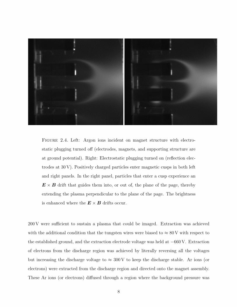
Figure 2.4. Left: Argon ions incident on magnet structure with electro-
static plugging turned off (electrodes, magnets, and supporting structure are
at ground potential). Right: Electrostatic plugging turned on (reflection elec-
trodes at 30 V). Positively charged particles enter magnetic cusps in both left
and right panels. In the right panel, particles that enter a cusp experience an
E ×B drift that guides them into, or out of, the plane of the page, thereby
extending the plasma perpendicular to the plane of the page. The brightness
is enhanced where the E ×B drifts occur.
200 V were sufficient to sustain a plasma that could be imaged. Extraction was achieved
with the additional condition that the tungsten wires were biased to ≈ 80 V with respect to
the established ground, and the extraction electrode voltage was held at −660 V. Extraction
of electrons from the discharge region was achieved by literally reversing all the voltages
but increasing the discharge voltage to ≈ 300 V to keep the discharge stable. Ar ions (or
electrons) were extracted from the discharge region and directed onto the magnet assembly.
These Ar ions (or electrons) diffused through a region where the background pressure was
8

Figure 2.5. Electrons incident on magnet structure. Left: Electrostatic plug-
ging turned off. Right: Electrostatic plugging turned on (−200 V). Right: The
E ×B drift caused the plasma to reach and pass in front of the ends of the
magnets closest to the camera.
relatively high (120 mTorr), with a mean free path of ≈ 0.05 cm. The Ar ions (or electrons)
collisionally excited residual gas atoms, which primarily consisted of Ar atoms.
An ST-7XMEI SBIG CCD camera was employed to record light emitted by de-
excitations, using typical integration times of 2 to 3 minutes. The plasma was imaged with
electrostatic plugging either turned off or turned on. Images that represent the behavior
observed are shown in in Fig. 2.4 for Ar ion extraction and Fig. 2.5 for electron extraction
from the discharge region.
2.3. Results
For the conditions of the experiment presented here, the charged particle trajectories
are observed to follow magnetic field lines and to be confined to regions of low magnetic
field strength. This behavior is observed by inspecting Figs. 2.2, 2.4, and 2.5. Charged
9

particles that are incident on the magnet assembly near the middle of the magnet edges,
away from their corners, and have trajectories that are nearly parallel to the planes of the
magnets enter the regions of cusping magnetic fields. Experimental results associated with
electrostatic plugging of the magnetic field cusps are shown in the right panels of Fig. 2.4
and Fig. 2.5. Electrostatic plugging of the magnetic field cusps further modifies charged
particle trajectories and is observed to cause an E ×B drift that guides charged particles
into or out of the plane of the page.
10

CHAPTER 3
ARTIFICIALLY STRUCTURED BOUNDARY FOR A HIGH PURITY ION TRAP OR
ION SOURCE
3.1. Introduction
In the application of ion sources for accelerator physics, plasma physics, or plasma
processing purposes, a clean source of ions is desirable when unwanted sputtered contam-
ination is detrimental for the experiment at hand or for the ion source assembly itself. In
addition, in the accumulation of rare species of ions or antimatter particles, good confine-
ment is particularly important due to the limited availability of the particles being trapped.
Ions within an ion source that impinge on a surrounding material surface can alter the phys-
ical properties of the surface. Furthermore, ion sources that employ reactive metals can
require frequent service intervals. The study presented here proposes a configuration that
can minimize the interaction of a plasma with material surfaces.
An artificially structured boundary (ASB) is described here as a material boundary
that produces electrostatic and magnetostatic fields for the purpose of modifying charged
particle trajectories when charged particles approach the boundary. Such an ASB is consid-
ered here to form a periodic set of cusping magnetic fields with electrostatic potential barriers
at the location of the magnetic field cusps. An ASB that produces purely magnetic fields,
without the electrostatic barriers, is described in [2]. Two properties of such an arrangement
are notable: (1) The ASB is capable of simultaneously reflecting charged particles of either
sign of charge, but only when the particles are incident at shallow angles. (2) A nearly
field free region occurs away from the ASB so that the field only modifies charged particle
trajectories close to the material boundary. Charged particle trajectories that are normal
to the ASB can escape through magnetic field cusps if no electrostatic plugging is present.
Preliminary experimental research has been reported previously in which a plasma interacts
with a segment of an ASB with electrostatic plugging [9]. Also, theoretical research has been
reported on possible applications of an ASB for lining an electrostatic storage ring [10] and
11

for bounding a confined plasma [11]. The current study assesses the effect that incorporating
electrostatic plugging of the magnetic field cusps can have on the confinement of charged
particles of a single sign of charge. The configuration may serve to confine a two-species
plasma, with the first species confined by the ASB and the second, oppositely signed species,
confined by the space charge of the first species [11].
In Sec. 3.2, the fields employed for confinement are described. A normalization scheme
is developed and normalized equations of motion are derived. The method of solution is also
presented in Sec. 3.2. Results are presented in Sec. ??. Concluding remarks are presented
in Sec. 3.4.
3.2. Theory
The current study considers the interaction of a single charged particle with an ASB.
The effects due to the collective nature of plasmas are not taken into account here. Charged
particle trajectories near an ASB are determined by solving Newton’s second law. Figure 3.1
depicts the characteristics of the simulation environment.
The magnetic field developed in [12] is used here, except that (1) the magnetic field
dependence on the coordinates is changed, and (2) the strength of the field is defined by the
conditions necessary for magnetic confinement. Such a field has the form [12]
(1) B(x, y, z) = B0βt
(xS,y
S,z
S
),
with
(2) βt(xn, yn, zn) =N∑i=1
ηiβ(xn, yn − (i− 1)∆yn, 0),
and
(3) β(xn, yn, zn) =− cos(2πxn) sinh(2πyn)
cos(4πxn)− cosh(4πyn)x+
sin(2πxn) cosh(2πyn)
cos(4πxn)− cosh(4πyn)y.
Here rn = xnx + yny + znz = rS
; β(xn, yn, zn) describes the direction of the magnetic field
created by a planar array of current carrying wires that has a spatial period S, that is infinite
in z dimension and coincides with the y = 0 plane; and ηi assigns relative current factors for
each of the N(=10) planar arrays that are stacked ∆yn apart. η1 = η10 = 1.27 and ηi = 1 for
12

2 ≤ i ≤ 9. B0 is approximately equal to the magnitude of the magnetic field at the center
of the anode gap. An expression for B0 will be developed in a later section.
The electric field used for electrostatic plugging of the magnetic field cusps is obtained
by numerically computing the electrostatic potential φ(x, y, z) and then using E(x, y, z) =
−∇φ(x, y, z). The numerical computation of φ is described below.
Normalization
Consider a collisionless, non-drifting, unmagnetized plasma that follows a Maxwellian
velocity distribution. From this point onward, an ensemble of charged particles is loosely
referred to as a plasma. T is the temperature, in units of energy, associated with the
Maxwellian distribution and m is the mass of a plasma particle. Assume that the plasma is
composed of a single species of charged particles, each of which has a positive charge q (e.g.,
q = 2e for a doubly ionized positive species, and e is the electronic charge). In what follows,
the quantities m, q, S, and 3T/2 are employed to carry out a normalization procedure.
S is the spatial period of the magnetic field, and 3T/2 is the average kinetic energy per
particle in a Maxwellian source of particles. The normalized parameters are tn = tS
√3T2m
,
rn = rS
, vn = v√
2m3T
, an = a2mS3T
, Bn = BSq√
23mT
, En = E 2Sq3T
, and φn = 2qφ3T
, which are
the dimensionless normalized time, position, velocity, acceleration, magnetic field, electric
field, and electric potential, respectively. Newton’s second law for a charged particle that
experiences a Lorentz force is
(4) an = En + (vn ×Bn),
when written in terms of the normalized parameters. The normalized electric field is
(5) En = −∇φn(xn, yn, zn).
Consider a positive charged particle in a region with electrostatic potential φ, which is
positive or zero everywhere accessible to the particle. In particular, consider the electrostatic
potential present in the ASB described in Fig. 3.1, where φ = φ0 at the center of the anode
gap between electrodes labeled by V1. The electrostatic potential energy barrier, U0 = qφ0,
13

Electrodes
V0
V2
V1
S
Δyn
Current-carrying
wires
α
vx
vo
vy
+I +I -I -I
φ0 B0
βt
η1
η2
ηi
Figure 3.1. Simulation environment representing two periods of a planar
ASB. Ions are confined to the region below the ASB (yn < 0). The lower
edge of the ASB is located at yn = 0. The dots mark the positions of the
current carrying wires, with current that alternates in sign from one column
of wires to the next, ±I. Magnetic field cusps are produced with the direc-
tion of the magnetic field labeled by βt. The electrodes are marked by lines,
which represent their lengths and locations in the simulation environment.
The current carrying wires and the electrodes are infinite in extent in the z
dimension. The electrostatic potential energy barrier is located in the region
0.5 ≤ yn ≤ 0.75, at the location of V1. V0 and V2 are at ground potential. φ0 is
the electric potential at the center of the anode gap, where the magnetic field
has a magnitude B0. See Eq. (2) for details regarding ηi, and ∆yn.
14

reflects charged particles that start at zero potential with less kinetic energy than is required
to overcome the potential energy barrier. Define the ratio of the electrostatic potential energy
barrier, at the location of φ0, to the average kinetic energy of a plasma particle to be the
normalized potential barrier,
(6) φn0 =2qφ0
3T.
The Larmor radius, RL, is used to specify a condition for magnetic confinement.
At the center of the anode gap, the magnetic field has a magnitude specified by B0, so
that RL = mvpqB0
. Here vp is the magnitude of the velocity component perpendicular to the
direction of the magnetic field at the location of B0. In order for a charged particle to
experience magnetic confinement in the anode gap, its Larmor radius must be much smaller
than the space between two adjacent columns of wires, i.e. RL S4. Let the average thermal
energy be available to a plasma particle’s motion perpendicular to the magnetic field. In
such case 32T = m
2v2
p, which leads to
(7) B0 =
√3mT
qRL
.
With the magnetic field given by Eq. (1), and defining an inverse normalized Larmor radius
δ = SRL
, the normalized magnetic field becomes
(8) Bn =√
2δβt(xn, yn, zn),
where δ 4 is considered necessary for magnetic confinement.
Equations of Motion
The equations of motion are obtained from Eqs. (4), (5), and (8). For the planar
system considered in the current study, the fields are completely independent of the z-
coordinate. Therefore, the equations of motion become
(9) x′′n(tn) = Enx −√
2δ (z′n(tn)βty) ,
(10) y′′n(tn) = Eny +√
2δ (z′n(tn)βtx) ,
15

and
(11) z′′n(tn) =√
2δ (x′n(tn)βty − y′n(tn)βtx) .
Here, βtx, Enx and βty, Eny are the x and y components of βt and En, respectively, and the
notation x′n(tn) is the derivative of the normalized position with respect to normalized time.
The equations of motion (Eqs. (9)-(11)) were solved simultaneously to obtain parametric
trajectories in three dimensions.
Method of Solution
The initial conditions for the simulation of trajectories were obtained in the following
manner. Assume that the plasma has a temperature T associated with a Maxwellian velocity
distribution. Taking the present normalization into account, the initial components of the
velocity vector are obtained via
(12) vn0,i =
√2
3(−2 ln[R1i])
12 cos(2πR2i)
with i = x, y, or z. Equation (12) represents random components of the initial velocity
vector sampled from a Maxwellian distribution [13, 14], where Rji are all independent ran-
dom numbers with a uniform distribution between zero and one. The initial conditions
are obtained from the velocity vector vn0 = vn0,xx + vn0,yy + vn0,zz and position vector
rn0 = R[−1, 1]x− 3y + 0z, where x, y, and z are Cartesian unit vectors and R[x1, x2] is a
random number with a uniform distribution between x1 and x2. Note that the motion in the
y dimension takes charged particles towards [away from] the ASB when the velocity compo-
nent in the y dimension is positive [negative]; see Fig. 3.1. Consequently, the initial velocity
component in the y direction is calculated as prescribed by Eq. (12), and its absolute value
is used so that all charged particles initially travel toward the ASB. The initial x coordinate
is sampled over two full periods of the simulation environment, which directly corresponds
to the simulation region presented in Fig. 3.1. Additionally, two periods were chosen for the
simulation region in order to allow for a large sampling of the phase-space but not so large
that trajectories with glancing angles dominate the statistics obtained.
16

Taking advantage of the periodicity of the system, the electrostatic potential was
computed for a region that is 0.5S wide in the x dimension and 5.0S long in the y dimension
and then the solution was repeated in the x dimension to complete the simulation region.
The top of the simulation boundary corresponds to yn = 1 and the bottom to yn = −4.
The electrode labeled V0 starts at yn = 0 and ends at yn = 0.5, the electrode labeled V1
starts at yn = 0.5 and ends at yn = 0.75, and the electrode labeled V2 starts at yn = 0.75
and ends at yn = 1.0, with one grid unit between adjacent electrodes. The electrostatic
potential was computed using a finite differences sequential over-relaxation method [15].
In the calculation of the electrostatic potential, there are 40 grid units per period-lengths.
Values were specified for applied normalized potentials Vn0, Vn1, and Vn2 to establish the
boundary conditions at the electrode locations. Vn0 and Vn2 were set to ground potential,
Vn0 = Vn2 = 0, whereas Vn1 was biased to a positive value that was iteratively increased
until a chosen value for φn0 was reached at the center of the anode gap. The electrostatic
potential was obtained by first assigning values to the boundary regions where electrodes
are located, then applying the finite difference sequential over-relaxation algorithm to the
internal points, and assigning values to the remaining boundary points by requiring that the
derivative normal to the boundary be zero. Such a procedure was carried out a sufficient
number of times so that the difference in calculated normalized potential values from one
iteration to the next was less than 1× 10⁻⁵ for all internal points.
The equations of motion were solved simultaneously via a “leap-frog” numerical ap-
proach (see, for example [16]). The time-step size was adjusted until the energy throughout
the simulation was conserved to within 1% of the initial energy for all trajectories, during
code development on a desktop computer. The same code was submitted for batch process-
ing on a supercomputer. Some of the trajectories obtained from the supercomputer were
also chosen and checked for energy conservation to within 1%.
3.3. Results
A parameter study for a single-species plasma can be performed in terms of the
normalized parameters φn0 and δ. Figure 3.2 was obtained by solving Eqs. (9)-(11) with
17

Figure 3.2. Simulation that represents a two period segment of an ASB. The
different shades show trajectories with φn0 = 1 and δ = 1000 (black), δ = 100
(dark gray), and δ = 20 (light gray). The trajectory calculation is terminated
when a particle reaches yn = 0.75.
φn0 = 1 and with δ =1000 (1000 trajectories), δ =100 (2000 trajectories) or δ =20 (3000
trajectories) and by plotting the x and y components of the position vector in a parametric
form. A different number of trajectories was chosen for the purpose of achieving the contrast
18

Figure 3.3. Simulation that represents a two period segment of an ASB.
The different shades show trajectories with δ = 20, and φn0 = 0.5 (light gray)
and φn0 = 5 (black). The trajectory calculation is terminated when a particle
reaches yn = 0.75.
in the figure. Figure 3.2 shows the general behavior of charged particle trajectories near
an ASB as the inverse normalized Larmor radius δ is varied. Charged particle trajectories
were also calculated in a similar manner but keeping the inverse normalized Larmor radius
19

••••••••••••
•••••
••••
•
••••
•
•
•
••
•
••
•
••
•
•
•
•
•••
•
•
•
•••
•
•
•
•
•
•
••
•
•
••
•••
••••
•
•
••
••
•
••••
•
•
•
•••
•
••••••••
•••••ääääääääääääääääääääääääääääääääää
äääää
ää
ä
ä
ä
ä
ää
ä
ä
ä
ä
ä
ä
ä
ä
ää
ää
ä
ä
ää
äääää
ääääääääääääääääääääääääääääääää
∆ = 10 H•L∆ = 20 H L∆ = 40 H L
H•L 2.00 %
H L 1.02 %
H L 0.57 %
-0.2 -0.1 0.0 0.1 0.20
10
20
30
40
50
xn
Num
bero
fC
ount
s
Figure 3.4. Profile of the spatial distribution of charged particles that
reached yn ≥ 0.75 after entering a cusp and overcoming the electrostatic po-
tential barrier. The distribution of particles at yn ≈ 0.75 is for φn0 = 1 and
δ = 10, 20, and 40. The data series are labeled according to the parameter
varied, and the corresponding percentages of particles that reached yn ≈ 0.75
are indicated. The total number of trajectories simulated for each of these
plots was 100,000.
constant and varying the normalized electrostatic potential barrier φn0. The results are
shown in Fig. 3.3.
The trends observed are (1) increasing the magnetic field sufficiently can effectively
reflect charged particles away from most of the solid material and (2) increasing the electro-
static plugging sufficiently can reflect charged particles that would otherwise escape through
the magnetic field cusps. The latter trend is, of course, directly affected by the kinetic energy
20

äääääääääääääääää
ääääää
ä
ä
ä
ä
ä
äää
ä
ä
ä
ä
ä
ä
ä
ä
ä
ä
ä
ä
ä
ää
ää
ä
ä
ä
ää
ä
ä
ä
ää
ä
ä
ää
äää
äää
ääää
ää
ä
ääääääää
äää
ääääääääääääää•••••••••••••••••••••••••••••
••••••••••
•••••••••
•
••••••
•••••••••
••••••••••••••••••••••••••••••••••••
Φn0 = 0.5 H LΦn0 = 1.0 H LΦn0 = 2.0 H•L
H L 2.23 %
H L 1.02 %
H•L 0.25 %
-0.2 -0.1 0.0 0.1 0.20
20
40
60
80
100
xn
Num
bero
fC
ount
s
Figure 3.5. Profile of the spatial distribution of charged particles that
reached yn ≥ 0.75 after entering a cusp and overcoming the electrostatic po-
tential barrier. The distribution is for δ = 20 and φn0 = 0.5, 1, and 2. The
data series are labeled according to the parameter varied, and the correspond-
ing percentages of particles that reached yn ≈ 0.75 are indicated. The total
number of trajectories simulated for each of these plots was 100,000.
of the charged particles, and those particles that escape lie in the high energy tail of the
speed distribution. In the simulations, the trajectories were terminated when the particles
reached yn ≥ 0.75 (past the electrostatic potential barrier), or yn ≤ −3, or |xn| ≥ 1, or
|zn| ≥ 5. However, Figs 3.2 and 3.3 only show a region defined by yn ≤ 1, yn ≥ −1.5, and
|xn| ≤ 1 primarily to observe the modification of charged particle trajectories when charged
particles approach the ASB. When a particle reached yn ≥ 0.75, its position vector was
recorded. The x component of the position vector for each of these particles was evaluated
21

with respect to the center of the particular cusp that each of these entered and was assigned
to a bin. There were 100 total bins for half of a spatial period in the simulation. Figures 3.4
and 3.5 show the data from 100,000 trajectories obtained by such a procedure. Figure 3.4
presents the spatial profile of the particles that reached yn ≈ 0.75 for different values of the
magnetic field/Larmor radius. Figure 3.5 is identical except that the magnetic field is fixed
and the electrostatic potential barrier is varied. The solid curves in Figs. 3.4 and 3.5 are
there to help distinguish the general trend that each of the data sets follow. The data series
are labeled according to the parameter varied, and the corresponding percentage of particles
that escaped confinement is shown. The plots show the most probable location through
which particles can escape. Good confinement is defined here as the set of conditions that
minimize the interaction of charged particles with the solid material. In the present study,
magnetic confinement becomes apparent when the Larmor radius is smaller than 0.2 times
the spatial period. The effect of electrostatic plugging is observed in Fig. 3.5. When the
average thermal energy is less than the height of the electrostatic potential barrier, bet-
ter confinement is achieved. For φn0 > 5 and δ > 20 the number of particles that escape
confinement becomes negligible for the number of trajectories simulated in the present work.
3.4. Conclusion
An artificially structured boundary that produces electrostatically plugged magnetic
field cusps has been presented as an alternative way to confine charged particles or plasma
for ion source applications. Accumulation and confinement of highly pure or rare ions could
benefit by decreased particle loss due to particle-solid material interaction. An ASB produces
fields near the solid material boundary, and a nearly field free region exists away from the
ASB. Charged particles can be confined by suitable adjustment of the applied electric and
magnetic fields.
22

CHAPTER 4
SPACE-CHARGE-BASED ELECTROSTATIC PLASMA CONFINEMENT INVOLVING
RELAXED PLASMA SPECIES
4.1. Introduction
Suppose that a hollow and evacuated sphere, which is made from a refractory metal
such as tungsten or tantalum, is heated to a temperature sufficient for thermionic electron
emission to occur from the interior surface. A non-drifting non-neutral electron plasma would
be produced within the interior of such a sphere. Under certain conditions, the space charge
of that electron plasma can be used to confine a positive-ion plasma or a positron plasma.
In the work presented here, the electrostatic potential and the density profile of
a surface-emitted or edge-confined non-drifting non-neutral single-species plasma are self-
consistently evaluated assuming a relaxed plasma. Next, the equilibrium of a two-species
plasma, with one plasma species confined by the space charge of the other, is self-consistently
evaluated. Each species is assumed to be relaxed to a Boltzmann density distribution. An
edge-confined plasma would be effectively unmagnetized, except near an outer boundary
where a confining electromagnetic field would reside [9]. One possibility is for the confining
electromagnetic field to consist of a spatially periodic sequence of magnetic cusps that are
plugged electrostatically. This is a case where a magnetic multipole would be superimposed
on an electric multipole of higher order. The spatial period and range of the field would be
much smaller than the dimensions of the plasma.
A motivation for the work presented here is the prospect of testing fundamental
symmetries between the properties of matter and antimatter such as the gravitational ac-
celeration symmetry [12, 17]. However, plasma drifts within nested Penning traps represent
a formidable problem for producing antihydrogen with sufficiently low kinetic energy to be
trapped in useful quantities for experimentation [3, 18, 19]. An antihydrogen atom is born
with the kinetic energy of its antiproton, and plasma drifts can increase the kinetic energy
of antiprotons. Therefore, an ideal plasma confinement approach for antihydrogen studies
23

Trapping Volume: Conceptual Model.
N
N
N
N
S
S
S
S
Trapping VolumeASBField
Region
+ I
– I
+ I
– I
ASB with Current-Carrying Wires ASB with Permanent Magnets
Magnetic Field
Magnetic Field
Figure 4.1. Conceptual model of a plasma trapping volume with a field free
region at its center. A plasma is envisioned to relax within the volume and be
“edge-confined” by a reflecting surface such as an ASB.
would avoid plasma drifts and be capable of providing long confinement times for a cold,
dense, non-drifting (e.g., non-rotating) plasma of any desired size.
A trapping volume that is lined with an ASB could confine a non-neutral plasma of
either sign of charge, see Fig. 4.1. The center of the trapping volume is essentially field free
and presents an ideal scenario for prolonged electrostatic trapping of an oppositely charged
species that is free of plasma drifts. Three-body recombination rates within a multiple
species plasma can be about a factor of 10 larger within an unmagnetized plasma relative to
a magnetized plasma, all other parameters being equal [20]. The trapping volume envisioned
here is potentially suitable for recombination experiments without plasma drifts.
In Sec. 4.2, a self-consistent computation of the electrostatic potential that occurs
within an unmagnetized non-neutral plasma under equilibrium conditions is developed. In
Sec. 4.3, a second plasma species is introduced and the resulting equilibrium of a two-species
plasma is evaluated. In Sec. 4.4, the conditions necessary for achieving space-charge-based
electrostatic confinement are discussed. Concluding remarks are found in Sec. 4.5.
24

4.2. Single-Species Non-Neutral Plasma
A region of space that contains electric field sources must satisfy Poisson’s equation.
Therefore, the electrostatic potential resulting from a Boltzmann distribution of charged par-
ticles can be obtained by solving Poisson’s equation and imposing the appropriate boundary
conditions according to the geometry of the problem. Poisson’s equation (in SI units) reads
(13) ∇2φ(r) = −ρ(r)
ε0,
where φ(r) is the electrostatic potential, ρ(r) is the charge density, and ε0 the vacuum per-
mittivity. Assume that a single-species plasma is in a steady-state equilibrium. Furthermore,
assume that the plasma is relaxed, such that the Boltzmann density distribution represents
the charged particle distribution in space [21]. Also, let the electrostatic potential be repre-
sented by the average of the local electrostatic potential (averaging over the discreteness of
the plasma constituents). The Boltzmann relation for the plasma density is
(14) n(r) = nse−q[φ(r)−φ(rs)]/T .
Here, ns is a known plasma density at rs, q is the charge of a plasma particle (e.g., q = −e for
an electron plasma where e is the unit charge), and T is the plasma temperature in energy
units. The plasma temperature is assumed to be temporally constant and spatially uniform.
Equation (13), becomes
(15) ∇2φ(r) = −qnsεoe−q[φ(r)−φ(rs)]/T .
At the location where the plasma density is specified (i.e., at rs), the electrostatic potential is
defined to be zero: φ(rs) = 0. By solving Eq. (15) for the electrostatic potential, the plasma
equilibrium can be obtained. In order to generalize the study, the equation is normalized by
introducing a dimensionless potential ψ(r) = qφ(r)/T , and defining the Debye length at rs
as λD =√ε0T/(q2ns). With these modifications the governing equation simplifies to
(16) ∇2ψ(r) = −e−ψ(r)
λ2D
.
Equation (16) is solved for spherical, cylindrical, and planar geometries.
25

(1) For the spherical geometry, a system that has spherical symmetry is assumed. Let
r denote the radial coordinate of a spherical coordinate system. The governing
equation reads
(17)2
r
∂ψ
∂r+∂2ψ
∂r2= −e
−ψ
λ2D
.
(2) For the cylindrical geometry, a system is assumed that has infinite length in the
axial dimension and is cylindrically symmetric. Let r denote the radial coordinate
of the cylindrical system. The governing equation in cylindrical coordinates is
(18)1
r
∂ψ
∂r+∂2ψ
∂r2= −e
−ψ
λ2D
.
(3) For the planar geometry, assume that the system is contained between two infinite
planes. Let the variable r be defined as a Cartesian coordinate normal to the
planes. A system that has mirror symmetry about r = 0 is assumed. In this case,
the governing equation is
(19)∂2ψ
∂r2= −e
−ψ
λ2D
.
In the previous three equations, ψ is a function of the variable r, ψ = ψ(r). The notation
has been suppressed for brevity.
Equations (17), (18), and (19) are combined into a single equation. By introducing
a coefficient of the form (α − 1)/r in place of the term multiplying the first partial deriva-
tive, and changing variables to the spatial coordinate rn = r/λD, the following equation is
obtained:
(20)(α− 1)
rn
∂ψ(rn)
∂rn+∂2ψ(rn)
∂r2n
= −e−ψ(rn).
Here, α takes the value of 1, 2, or 3 for the planar, cylindrical, or spherical geometry,
respectively. Thus, Eqs. (17), (18), and (19) are simultaneously represented by Eq. (20) in
terms of the normalized coordinate rn.
26

Boundary Conditions
The symmetry of the charge distribution dictates a set of mixed boundary conditions.
(1) Neumann Boundary Condition
The electric field is zero at the origin:
(21)
[∂φ(r)
∂r
]r=0
=
[∂ψ(rn)
∂rn
]rn=0
= 0.
(2) Dirichlet Boundary Condition
The electrostatic potential is defined to be zero at the plasma edge:
(22) φ(rmax) = ψ(rn,max) = 0.
Here, the plasma edge is located at rmax and at rn,max = rmax/λD, where λD is the Debye
length at the plasma edge. The plasma diameter, or thickness in the planar geometry,
is 2rmax. The method by which the plasma is produced, sustained, and confined is not
considered here. The description is only applicable for the region 0 ≤ r ≤ rmax.
Finite Differences
A finite-differences computational approach has been used to predict plasma equilibria
in nested-well and single-well Malmberg-Penning traps [3, 22]. Equation (20) is solved using
a finite-differences approach. Written in terms of finite differences, the first partial derivative
of a general function, f(x, y, z), with respect to x (in symmetrical form) becomes:
(23)∂f(x, y, z)
∂x≈ f(x+ ∆x, y, z)− f(x−∆x, y, z)
2∆x.
The second partial derivative is
(24)∂2f(x, y, z)
∂x2≈ f(x+ ∆x, y, z) + f(x−∆x, y, z)
(∆x)2− 2f(x, y, z)
(∆x)2.
In principle, this recipe can be used to represent any second order partial differential
equation. Applying the finite-differences approach to Eq. (20) gives, after some algebraic
manipulations,
ψ(rn) =ω∆r2
n
2
[(α− 1)
rn
ψ(rn + ∆rn)− ψ(rn −∆rn)
2∆rn
27

+ψ(rn + ∆rn) + ψ(rn −∆rn)
∆r2n
+e−ψ(rn)]− (ω − 1)ψ(rn),(25)
where the left-hand side represents the new value each iteration, and the normalized grid
spacing is ∆rn = ∆r/λD. ω is introduced for the purpose of reducing computation time [15].
Equation (25) is implemented using a sequential over-relaxation method, with ω having a
value in the range 1 ≤ ω < 2 [22].
Self-Consistent Solution
A computer program was developed to solve for the normalized electrostatic potential
ψ using the finite-differences approach. The parameter ω and the number of iterations were
chosen to achieve the desired convergence. The self-consistent computation of the electro-
static potential was achieved by iteratively solving for the electrostatic potential according to
Eq. (25). All computations were run until the absolute difference between one iteration and
the next was less than 10−10 at every grid point. It has been reported that if the grid spacing
is on the order of, or smaller than, the Debye length, code instabilities are reduced, and the
convergence of a solution is more likely to be achieved [23]. The computation assigned at
least three grid points per Debye length for rmax λD and significantly more grid points
(≈ 50) per Debye length for values of rmax ≈ λD.
Figure 4.2 shows typical profiles of the electrostatic potential. The three plots cor-
respond to the planar, cylindrical, and spherical geometries (α = 1, 2, and 3, respectively).
The non-neutral plasma generates an electrostatic potential that has an extremum at the
center of each geometry (at rn = 0).
In Fig. 4.3, radial profiles of the normalized density function, e−ψ, are shown. The
profiles are for a spherical geometry, α = 3, with rn,max = 5, 10, 20, and 30. The non-
neutral plasma density has a minimum at the geometric center of the system. The behavior
of the plasma distribution in the vicinity of the boundary is observed to change in a more
pronounced manner as the value of rn,max increases, behavior that agrees qualitatively with
previous results for magnetized non-neutral plasmas [24].
28

0.0 0.2 0.4 0.6 0.8 1.0
rn
rn,max0
2
4
6
8
ΨElectrostatic Potential Profile
Figure 4.2. Typical radial profile of the normalized electrostatic potential.
The plots are for rn,max = 100 and α = 1 (solid), 2 (long dash), 3 (short dash).
The normalized electrostatic potential difference between the center and the
boundary is 7.6 for α = 1, 7.2 for α = 2, and 6.8 for α = 3.
0.0 0.2 0.4 0.6 0.8 1.0
rn
rn,max
0.2
0.4
0.6
0.8
1.0e-Ψ
Radial Plasma Distribution Profiles
Figure 4.3. Typical normalized density profiles. The plots are for α = 3 and
rn,max = 5 (dot-dashed), 10 (short dash), 20 (long dash), 30 (solid). Similar
profiles occur for other values of α.
29

æ
æ
æ
æ
æ
æ
æ
æ
æ
æ
ææ
æ
æ
æ
æ
à
à
à
à
à
à
à
à
à
à
àà
à
à
à
à
ì
ì
ì
ì
ì
ì
ì
ì
ì
ì
ìì
ì
ì
ì
ì
Α = 1 (è)
Α = 2 ()
Α = 3 (ì)
0 100 200 300 4000
2
4
6
8
10
rn,max
DΨ
0,Α
Normalized Electrostatic Potential Difference
Figure 4.4. Normalized electrostatic potential difference (between plasma
center and edge) for the three geometries. The solid lines are Eq. (26).
The behavior of the plasma has also been characterized by evaluating the normalized
potential at the geometric center of the volume in question. Recalling the boundary condition
ψ(rn,max) = 0, the normalized potential at rn = 0 is equal to the difference in normalized
potential between the geometric center and the boundary: ∆ψ0,α = ψ(0) − ψ(rn,max). The
value of the α subscript indicates the geometry being studied. Figure 4.4 shows how the
normalized potential difference, ∆ψ0,α, changes for increasing values of rn,max for planar,
cylindrical, and spherical geometries (α = 1, 2, 3). The value increases rapidly for small
values of rn,max and increases at a much slower rate for larger values of rn,max. Notice that
values exceeding 10 are predicted. Such large values indicate that it should be possible to
confine a second species of particles with opposite sign of charge within the electrostatic
potential well created by the first species, with both species having the same temperature
and charge state. Such a possibility is considered in Sec. 4.3.
The numerical results in Fig. 4.4 were fitted by an analytical expression. The approx-
imate analytical expression obtained for the normalized electrostatic potential difference
30

between the origin at rn = 0 and the boundary at rn,max is
(26) ∆ψ0,α = ln[(rn,max)0.217α0.139
]+W
(r2n,max
2α
).
Here, W (x) is the product logarithm function, which satisfies the equation x = W (x) exp [W (x)].
The last term on the right of Eq. (26) is the functional dependence that is expected in the
asymptotic limit of large rn,max. In such a limit, the density is spatially constant, except near
the plasma edge, where the variation is ignored, see Appendix B. Equation (26) agrees with
numerical results to within 1% for 30 ≤ rn,max ≤ 440 and to within 15% for 1 ≤ rn,max ≤ 30.
As a specific case, consider the electrostatic potential generated for rn,max = 100 and α = 3.
In such a case, ∆ψ0,α has a value of 6.85, and a 1 eV (temperature) electron plasma generates
an electric potential difference between the plasma edge and center of 6.85 V.
4.3. Two-Species Plasma
Consider a surface-emitted or edge-confined electron plasma that follows a Boltzmann
distribution as described in Sec. 4.2. An electrostatic potential energy well is created for
positive particles. Assume that a positive plasma species, such as a positive-ion or positron
plasma, is introduced near the center of the electron plasma. The charge density is ρ(r) =
−en−(r) + Zen+(r). Z represents the average charge state of the positive plasma particles.
The first term on the right-hand side refers to the electron plasma, which follows a Boltzmann
density profile of the form n−(r) = n0−exp(e[φ(r) − φ(rs)]/T−). The second term refers to
the positive plasma that is confined by the electrostatic potential well created by the space
charge of the electron plasma. The positive plasma is also assumed to follow a Boltzmann
distribution: n+(r) = n0+exp(−Ze[φ(r)− φ(0)]/T+). Poisson’s equation is
(27) ∇2φ(r) = − 1
ε0
[−en0−e
e[φ(r)−φ(rs)]T− + Zen0+e
−Ze[φ(r)−φ(0)]T+
],
where n−(rs) = n0− and n+(0) = n0+ are known densities of the respective plasma species.
Let Nn = Zn0+/n0− and Tn = ZT−/T+. Nn is the positive plasma charge density at the
center of the configuration normalized by the magnitude of the electron charge density at
the edge. Tn is the average charge state of the positive plasma particles multiplied by the
31

ratio of the electron temperature to the temperature of the positive species. Write
(28) ∇2φ(r) = −en0−
ε0
[−e
e[φ(r)−φ(rs)]T− +Nne
−eTn[φ(r)−φ(0)]T−
].
Introduce the normalized electrostatic potential, ψ(r) = eφ(r)/T−, with φ(rs) = 0, where rs
defines the boundary of the system:
(29) ∇2ψ(r) = −e2n0−
ε0T−
[−eψ(r) +Nne
−Tn[ψ(r)−ψ(0)]].
Define the Debye length at the boundary of the electron plasma as λ2D− = (ε0T−)/(e2n0−)
and scale the coordinates with respect to this quantity. Now,
(30) ∇2ψ(rn) = eψ(rn) −Nne−Tn[ψ(rn)−ψ(0)],
where rn = r/λD− is the normalized radial coordinate and ψ(0) is the value of the normalized
electrostatic potential at the center of the system. The Laplacian can be replaced by the
left-hand side of Eq. (20). The boundary conditions for the two-species plasma are identical
to those for the single-species plasma computations presented in Sec. 4.2, namely, Eqs. (21)
and (22).
A finite-differences approach was used to self-consistently evaluate the properties of
the plasma system. The shape of the electrostatic potential profile must now adjust to
include the effect of the positive species occupying the central region. Comparing Eq. (30)
to Eq. (20), one can see that Eq. (25) is applicable here, except that the density term becomes
(31) e−ψ(rn) → Nne−Tn[ψ(rn)−ψ(0)] − eψ(rn).
The computer program developed to solve for the normalized electrostatic potential
for a two-species plasma configuration is similar to the one used for Sec. 4.2, except that it
was adapted to include the density term for the second plasma species. The number of grid
points was determined by the smallest Debye length (smallest of the two species). At least
three grid points per such Debye length were used. The normalized electrostatic potential
was iteratively computed in a self-consistent manner until the absolute difference between
one iteration and the next was less than 10−10 at every grid point. Initial results indicate that
32

Increasing Positive Species Density
0.2 0.4 0.6 0.8 1.0
rn
rn,max
5
4
3
2
1
ΨNormalized Electrostatic Potential
+
+
+
_
_
_
Increasing Positive Species Density
0.0 0.2 0.4 0.6 0.8 1.0
rn
rn,max
0.0050.010
0.0500.100
0.5001.000
TwoSpecies Plasma Distribution
FIG. 5. Electrostatic potential of a two-species plasma (top). Self-consistent distributions of the
two plasma species (bottom) in logarithmic scale. The ratio of the temperatures is held constant
so that Tn = 5. The densities are varied: Nn = 0.004 (dashed), 0.04 (dot-dashed), 0.4 (solid).
The arrows indicate the trend that the system follows as the density of the positive plasma is
increased. The normalized distributions are n−(rn)/n0− , which are labeled by minus signs (–), and
n+(rn)/n0− , which are labeled by plus signs (+). The corresponding plot styles are for the two
distributions for a given value of Nn. rn,max is fixed at 30.
21
Figure 4.5. Normalized electrostatic potential of a two-species plasma (top).
Self-consistent distributions of the two plasma species (bottom) in logarithmic
scale. The plots are for, Tn = 5, rn,max = 30, and Nn = 0.004 (dashed),
0.04 (dot-dashed), 0.4 (solid). The arrows indicate the trend that the system
follows as Nn is increased. In the lower panel of this figure and Figs. 4.6-
4.8, the normalized distributions are n−(rn)/n0− , which are labeled by minus
signs (–), and Zn+(rn)/n0− , which are labeled by plus signs (+). Thus, each
matching pair of plots are the normalized distributions for the negative and
positive plasma species.
33

Increasing Positive Species Temperature
0.2 0.4 0.6 0.8 1.0
rn
rn,max
5
4
3
2
1
0Ψ
Normalized Electrostatic Potential
Increasing PositiveSpecies Temperature
_
+
0.0 0.2 0.4 0.6 0.8 1.0
rn
rn,max0.00
0.01
0.02
0.03
0.04
0.05TwoSpecies Plasma Distribution
FIG. 6. Electrostatic potential of a two-species plasma (top). Self-consistent distributions of the
two plasma species (bottom). The relative densities are held constant at Nn = 0.02 and the tem-
perature is varied: Tn = 1 (solid), 15 (dot-dashed), and 30 (dashed). The positive species density
is low enough that the negative species distribution and the normalized electrostatic potential
change only slightly. Notice the self-consistent equal-temperature equilibrium, Tn = 1, plot. The
normalized distributions are n−(rn)/n0− , which are labeled by a minus sign (–), and n+(rn)/n0− ,
which are labeled by a plus sign (+). rn,max is fixed at 30.
22
Figure 4.6. Normalized electrostatic potential of a two-species plasma (top).
Self-consistent distributions of the two plasma species (bottom). The plots
are for Nn = 0.02, rn,max = 30, and Tn = 1 (solid), 15 (dot-dashed), and 30
(dashed). The ± labels are defined in Fig. 4.5.
the electrostatic potential is similar for different geometries even when the positive plasma is
introduced. Only computations pertaining to a spherically symmetric system are presented
throughout the remainder of this chapter. The results obtained for cylindrically symmetric
system are presented in Chapter 5.
34

The depth of the electrostatic potential well tends to decrease as the positive plasma
charge density is increased. Such behavior is shown in Fig. 4.5. Also, for sufficiently high
charge densities of the positive plasma, both species approach the same charge density at the
center of the system. If the positive plasma charge density is sufficiently small, the electro-
static potential and density of the negative plasma are relatively unaffected by the presence
of the positive plasma. However, Fig. 4.6 shows that, for such a case, the volume occupied
by the positive plasma increases as the temperature of the positive plasma is increased, or
its average charge state is decreased.
The normalized electrostatic potential and distribution profiles for two plasma species
with equal temperatures and charge states under equilibrium conditions are shown in Fig. 4.7.
Notice that for sufficiently high charge densities of the positive plasma, the system reaches
neutrality near the center of the system. When the charge density of the positive plasma is
sufficiently low, there exists a state of partial neutralization. Figure 4.8 shows the minimum
positive species charge density at which the system achieves approximate neutrality at the
center of the system for different temperatures or charge states of the two plasma species.
The minimum neutral density decreases as the positive plasma temperature is lowered or its
average charge state is increased.
4.4. Space-Charge-Based Electrostatic Confinement Conditions
Good confinement of the positive plasma species can be expected to occur when the
electrostatic potential energy well that is self-consistently created by the plasma is much
deeper than the temperature (in energy units) of the positive plasma species [25]:
(32) T+ Ze∆φ0.
Here, ∆φ0 = φ(rmax)− φ(0) is the ordinary (unnormalized) electrostatic potential difference
between the edge and the center of the configuration. It may also be possible to sustain the
positive plasma species, even when Eq. (44) is not satisfied, provided that sufficient fueling
35

Increasing Positive Species Density
0.2 0.4 0.6 0.8 1.0
rn
rn,max
5
4
3
2
1
0Ψ
Normalized Electrostatic Potential
_
_
+
+
+
0.0 0.2 0.4 0.6 0.8 1.0
rn
rn,max
0.001
0.0050.010
0.0500.100
0.5001.000TwoSpecies Plasma Distribution: Equal Temperatures
FIG. 7. Two plasma species with disparate densities and equal temperatures (Tn = 1). The density
of the positive species is varied so that Nn = 0.1 (dot-dashed), 0.01 (dashed), and 0.001 (solid).
In the lower figure, the matching pairs of plots correspond to the negative and positive plasma
species. The density of the negative plasma species is normalized to unity at the boundary of the
system, rn = rn,max, and self consistently adjusts to accommodate the positive plasma species. The
normalized distributions are n−(rn)/n0− , which are labeled by minus signs (–), and n+(rn)/n0− ,
which are labeled by plus signs (+). rn,max is fixed at 30.
23
Figure 4.7. Two plasma species with equal temperatures and charge states.
The plots are for Tn = 1, rn,max = 30, and Nn = 0.1 (dot-dashed), 0.01
(dashed), and 0.001 (solid). The ± labels are defined in Fig. 4.5.
and heating are used. In terms of a normalized quantity, the condition is written as
(33) ∆ψ+0,α =Ze∆φ0
T+
1.
∆ψ+0,α is the normalized electrostatic potential energy well depth that confines the positive
plasma, and the value of the subscript α is used to indicate the geometry considered. ∆ψ+0,α
is evaluated in Fig. 4.9. A value for ∆ψ+0,α is first obtained by employing the approximate
36

Increasing Positive Species Density
0.2 0.4 0.6 0.8 1.0
rn
rn,max
5
4
3
2
1
0Ψ
Normalized Electrostatic Potential
_
_
_
+
++
0.0 0.2 0.4 0.6 0.8 1.0
rn
rn,max0.00
0.01
0.02
0.03
0.04
0.05
0.06
TwoSpecies Plasma Distribution: Equal Densities
FIG. 8. Two plasma species with disparate temperatures and equal densities at the center of the
plasma system. The normalized temperature and normalized density (Tn, Nn) are; (1, 0.05)[solid],
(10, 0.0225)[dot-dash], (25, 0.0152)[long dash], and (40, 0.0145)[short dash]. The normalized tem-
peratures were chosen and the normalized densities were then adjusted to the lowest value at which
the two distributions have the same value at the center of the system. The normalized distributions
are n−(rn)/n0− , which are labeled by minus signs (–), and n+(rn)/n0− , which are labeled by a
plus signs (+). rn,max is fixed at 30.
24
Figure 4.8. Two plasma species with approximately equal charge densi-
ties at the center of the plasma system. The plots are for rn,max = 30 and
(Tn, Nn) = (1, 0.05)[solid], (10, 0.0225)[dot-dashed], (25, 0.0152)[long dash],
and (40, 0.0145)[short dash]. The normalized electron temperatures, Tn, were
chosen and the normalized positive plasma charge densities, Nn, were then ad-
justed to the lowest value at which the two distributions have approximately
the same value at the center of the system. The ± labels are defined in Fig. 4.5.
37

expression developed in Sec. 4.2 [Eq. (26)], which represents the limit Nn → 0. The result
is shown in Fig. 4.9 (top panel, dotted line). To explore the effect that Tn and Nn have on
∆ψ+0,α, this quantity was evaluated as a function of system size for two different values of
Tn and varying Nn values. It is found that the normalized electrostatic potential energy well
depth tends to decrease as the normalized charge density of the positive plasma is increased,
and to increase with normalized system size. However, for a sufficiently large normalized
size, the normalized well depth saturates to a value nearly independent of the normalized
size of the system. The normalized well depth is also found to increase with Tn.
Figure 4.10 shows ∆ψ0,α = ∆ψ+0,α/Tn = e∆φ0/T−, the normalized electrostatic
potential difference, evaluated in the saturated regime for several values of Tn and Nn. An
expression for the normalized electrostatic potential difference is readily derived by assuming
that the plasma is neutral at the center. The expression is
(34)∆ψ+0,α
Tn= ∆ψ0,α = − ln(Nn).
Inspection of Figs. 4.8 and 4.9 indicates that, for the spherical geometry, Eq. (34) is applicable
for rn,max & 200, 10−4 . Nn < 1, and 1 ≤ Tn ≤ 10. The close agreement between Eq. (34)
and the numerical values suggests that the saturated regime is an equilibrium in which a
neutral region forms. It is conjectured that the electric potential well depth in the two-species
plasma is given by the smaller of Eq. (26) and Eq. (34). The predicted electric potential
well depth can be used together with collision-based theory, such as that in Refs. [25, 26] to
evaluate space-charge-based electrostatic plasma confinement time scales.
4.5. Conclusion
A self-consistent computation of the electrostatic potential generated by an edge-
confined or surface-emitted non-neutral plasma that follows a Boltzmann density distribution
with planar, cylindrical, or spherical symmetry has been carried out. The electrostatic
potential profile, plasma density distribution, and the electrostatic potential well depth for
different values of the normalized (to the edge Debye length) plasma size have been evaluated.
Relatively deep electrostatic potential wells are predicted by the computation when the
38

0 50 100 150 200 250 300 3500
2
4
6
8
rn,max
Ψ0,3;T n1
0 50 100 150 200 250 300 3500
20
40
60
80
rn,max
Ψ0,3;T n10
FIG. 9. Electrostatic potential difference between the edge and the center of the system composed
of two plasma species which is plotted vs. system size. Top (bottom) plot shows the electrostatic
potential difference that a positive plasma experiences when the temperatures are equal, Tn = 1
(disparate, Tn = 10). Notice the difference in magnitude of the vertical axis. The different plot
styles are for Nn = 0.1 (solid), 0.01 (long dash), 0.001 (dash), 0.0001 (dot-dash). The dotted line
in the top figure illustrates the trend as Nn → 0.
25
Figure 4.9. Normalized electrostatic potential energy well depth for space-
charge-based electrostatic plasma confinement as a function of normalized sys-
tem size. The dotted line in the top panel is for Nn = 0 and Tn = 1. Top
(bottom) panel is for Tn = 1 (Tn = 10), and Nn = 0.1 (solid), 0.01 (long dash),
0.001 (dash), 0.0001 (dot-dashed).
plasma size is much greater than the Debye length. An approximate expression has been
fitted for the electrostatic potential well depth as a function of the normalized plasma size.
39

10-4 0.001 0.01 0.1 10
2
4
6
8
10
Nn
DΨ0,3
Figure 4.10. Normalized electrostatic potential difference for increasing nor-
malized charge density of the positive species. There are plot points for
rn,max = 300 and Tn = 1, 4, and 10, for each value of Nn, but the plot points
are indistinguishable. The solid line is Eq. (34).
A self-consistent computation has been carried out for a positive plasma that is con-
fined by the space charge of an edge-confined or surface-emitted electron plasma, with both
species following Boltzmann density distributions. The results also apply to a negative
plasma that is confined by the space charge of an edge-confined positive plasma such as a
positron plasma. The results presented for the two-species system pertain to a spherically
symmetric system, but are expected to be qualitatively applicable to planar and cylindrical
geometries. The two-species system has been characterized by varying normalized param-
eters, which include (1) the ratio of the plasma radius to the Debye length at the plasma
edge, (2) the ratio of the positive plasma charge density at the center of the system to that
of the electron plasma at the edge, and (3) the ratio of the temperatures multiplied by the
average charge state. The electrostatic potential profile and the charge density distribution
have been computed, and the cases explored indicate the following: (1) Increasing the charge
density of the positive plasma species decreases the depth of the electrostatic potential well.
(2) Increasing the temperature or decreasing the average charge state of the positive plasma
40

causes the positive plasma to occupy a larger volume. (3) An equilibrium is possible in which
the two plasma species have equal temperatures and equal charge states. (4) Approximately
equal charge densities of the two plasma species at the center of the system occurs for a
sufficiently high charge density of the positive plasma species, even when the temperatures
and charge states are equal.
The electrostatic potential well depth has been evaluated for the two-species system.
It has been found that, once the positive plasma is introduced, the electrostatic potential
well depth reaches a saturation regime when the normalized plasma size is sufficiently large.
41

CHAPTER 5
ELECTROSTATIC STORAGE RING WITH FOCUSING PROVIDED BY THE SPACE
CHARGE OF AN ELECTRON PLASMA
5.1. Introduction
In what follows, a study similar to that found in Chapter 4 is carried out for a cylindri-
cally symmetric system. A cylindrically symmetric system that employs space-charge-based
confinement is presented. Based on the study, propositions and remarks for constructing a
cylindrically symmetric experimental apparatus are made.
Several purely electrostatic systems can be employed to confine ion beams or drift-
ing ion plasmas, such as electrostatic storage rings, electrostatic ion beam traps, Kingdon
traps, and electrostatic beam guides [27, 28, 29, 30, 31, 32, 33, 5]. Confinement of charged
particles by purely electrostatic means is important when time-varying electro magnetic or
magnetostatic confinement interfere with the experiment at hand. A system is proposed here
for investigation of atomic physics processes in plasmas (e.g., processes characterized by the
interaction of trapped heavy ions and plasma electrons). A system is envisioned where a
hollow and evacuated cylinder, which is made from a refractory metal such as tungsten or
tantalum, is heated to a temperature sufficient for thermionic electron emission to occur
from the interior surface. A non-drifting, non-neutral electron plasma would be produced
within the interior of such cylinder, and an electrostatic potential well for positive particles
would be created by the space charge of the electron plasma. Similarly, suppose a cylindrical
beam line has an interior surface lined with an artificially structured boundary [2] so that
it confines an electron plasma. Under certain conditions, the space charge of that electron
plasma can be used to focus a positive-ion beam or drifting plasma; see Fig. 5.2. Note
that focusing is loosely defined here as the nominal effect of ion bunching towards a desired
region, and its definition is not the typical ion optics one.
The equilibrium of a two-species system, with one species confined by the space
charge of the other, is self-consistently evaluated. Each species is assumed to be radially
42
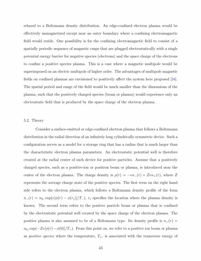
relaxed to a Boltzmann density distribution. An edge-confined electron plasma would be
effectively unmagnetized except near an outer boundary where a confining electromagnetic
field would reside. One possibility is for the confining electromagnetic field to consist of a
spatially periodic sequence of magnetic cusps that are plugged electrostatically with a single
potential energy barrier for negative species (electrons) and the space charge of the electrons
to confine a positive species plasma. This is a case where a magnetic multipole would be
superimposed on an electric multipole of higher order. The advantages of multipole magnetic
fields on confined plasmas are envisioned to positively affect the system here proposed [34].
The spatial period and range of the field would be much smaller than the dimensions of the
plasma, such that the positively charged species (beam or plasma) would experience only an
electrostatic field that is produced by the space charge of the electron plasma.
5.2. Theory
Consider a surface-emitted or edge-confined electron plasma that follows a Boltzmann
distribution in the radial direction of an infinitely long cylindrically symmetric device. Such a
configuration serves as a model for a storage ring that has a radius that is much larger than
the characteristic electron plasma parameters. An electrostatic potential well is therefore
created at the radial center of such device for positive particles. Assume that a positively
charged species, such as a positive-ion or positron beam or plasma, is introduced near the
center of the electron plasma. The charge density is ρ(r) = −en−(r) + Zen+(r), where Z
represents the average charge state of the positive species. The first term on the right hand
side refers to the electron plasma, which follows a Boltzmann density profile of the form
n−(r) = n0−exp(e[φ(r) − φ(rs)]/T−), rs specifies the location where the plasma density is
known. The second term refers to the positive particle beam or plasma that is confined
by the electrostatic potential well created by the space charge of the electron plasma. The
positive plasma is also assumed to be of a Boltzmann type. Its density profile is n+(r) =
n0+exp(−Ze[φ(r)−φ(0)]/T+). From this point on, we refer to a positive ion beam or plasma
as positive species where the temperature, T+, is associated with the transverse energy of
43

rn
zn
n0+
n0_
n0_
Artificially StructuredBoundary
Positive Ion Beam or Plasma
Electron Plasma
Electron Plasma
rn,max
Figure 5.1. Cross-sections of a segment of a cylindrical beam line. The
electron plasma is confined by an artificially structured boundary. The space
charge of the electron plasma creates an electrostatic potential that focuses a
positive-ion beam or drifting plasma.
the positive ion beam, or T+ is the characteristic temperature of the positive species when
it is referred to as a plasma.
Poisson’s equation is
(35) ∇2φ(r) = − 1
ε0
(−en0−e
e[φ(r)−φ(rs)]T− + Zen0+e
−Ze[φ(r)−φ(0)]T+
),
where n−(rs) = n0− and n+(0) = n0+ are known densities of the respective species. Let
Nn = Zn0+/n0− and Tn = ZT−/T+. Nn is the positive species charge density at the center
of the configuration normalized by the magnitude of the electron charge density at the edge.
Tn is the average charge state of the positive species multiplied by the ratio of the electron
44

temperature to the temperature of the positive species. Equation (35) can be written as
(36) ∇2φ(r) = −en0−
ε0
(−e
e[φ(r)−φ(rs)]T− +Nne
−eTn[φ(r)−φ(0)]T−
).
Introducing the normalized electrostatic potential, ψ(r) = eφ(r)/T−, with φ(rs) = 0, where
rs is the boundary of the system, gives
(37) ∇2ψ(r) = −e2n0−
ε0T−
(−eψ(r) +Nne
−Tn[ψ(r)−ψ(0)]).
Then defining the Debye length at the boundary of the electron plasma as λ2D− = (ε0T−)/(e2n0−)
and scale the coordinates with respect to this quantity produces
(38) ∇2ψ(rn) = eψ(rn) −Nne−Tn[ψ(rn)−ψ(0)],
where rn = r/λD− is the normalized radial coordinate, and ψ(0) is the value of the normalized
electrostatic potential at the center of the system. For a storage ring, in the limit of a large
radius, a cylindrical geometry is assumed. The Laplacian operator in Eq. (38) takes its usual
cylindrical form.
(39)1
rn
∂ψ(rn)
∂rn+∂2ψ(rn)
∂r2n
= eψ(rn) −Nne−Tn[ψ(rn)−ψ(0)].
Note that the system has been scaled with respect to the electron plasma Debye length.
However, quantities pertaining to the positive species can be obtained via the following
relationships:
(40) λ2D− = TnNn
ε0T+
e2Z2n0+
= TnNnλ2D+
and
(41) ψ+(rn) = −Tnψ(rn).
The notation ψ(rn) = ψ−(rn) could be used in Eqs. (37), (38), and (41), and note that
electron and positive species Debye lengths are specified with respect to the densities at the
boundary and the center of the system, respectively.
The boundary conditions for the two-species plasma are:
45

(1) Neumann Boundary Condition
(42)
[∂φ(r)
∂r
]r=0
=
[∂ψ(rn)
∂rn
]rn=0
= 0.
(2) Dirichlet Boundary Condition
(43) φ(rmax) = ψ(rn,max) = 0,
where rmax = rs and rn,max = rsλD−
.
A finite-differences approach was used to self-consistently solve Eq. (18) to calculate
the properties of the system when the two species are present [15]. The number of grid
points was determined by the smallest Debye length (smallest of the two species). At least
three grid points per such Debye length were used. The electrostatic potential was iteratively
calculated in a self-consistent manner until the absolute difference between one iteration and
the next was less than 10−10 for all grid points.
5.3. Results
For sufficiently high densities of the positive species, both species approach the same
charge density at the center of the system and the electrostatic potential well depth decreases
as the charge density of the postive species is increased. Such behavior is shown in the
Fig. 5.2. If the positive species charge density is sufficiently small, the electrostatic potential
generated by, and density of, the electron plasma are unaffected by the presence of the
positive species. However, Fig. 5.3 shows that as the temperature of the positive species is
increased, its distribution occupies a larger volume.
The normalized electrostatic potential and distributions profiles for two species with
equal temperatures and charge states under equilibrium conditions are now examined. Fig-
ure 5.4 shows a two-species system in which these have equal temperatures and charge states.
Notice that for sufficiently high charge densities of the positive species, the system reaches
neutrality near the center. When the charge density of the positive species is lower, there
exists a state of partial neutralization.
46

Increasing Positive Species Density
0.2 0.4 0.6 0.8 1.0
rn
rn,max
-5
-4
-3
-2
-1
ΨNormalized Electrostatic Potential
Increasing Positive Species Density
_
_
_
+
+
+
0.0 0.2 0.4 0.6 0.8 1.0
rn
rn,max
0.005
0.010
0.050
0.100
0.500
1.000Radial Distribution Profiles
Figure 5.2. Normalized electrostatic potential of a two-species system (top).
Self-consistent distributions of the two species (bottom) in logarithmic scale.
The plots are for, Tn = 5, rn,max = 30, and Nn = 0.004 (dashed), 0.04 (dot-
dashed), 0.4 (solid). The arrows indicate the trend that the system follows
as Nn is increased. In the lower panel of this figure and Figs. 5.3-5.5, the
normalized distributions are n−(rn)/n0− , which are labeled by minus signs (–),
and Zn+(rn)/n0− , which are labeled by plus signs (+). Thus, each matching
pair of plots are the normalized distributions for the negative and positive
plasma species.
47

Increasing Positive Species Temperature
0.2 0.4 0.6 0.8 1.0
rn
rn,max
-5
-4
-3
-2
-1
ΨNormalized Electrostatic Potential
Increasing Positive
Species Temperature
_
+
0.0 0.2 0.4 0.6 0.8 1.0
rn
rn,max0.00
0.01
0.02
0.03
0.04
0.05Radial Distribution Profiles
Figure 5.3. Normalized electrostatic potential of a two-species plasma (top).
Self-consistent distributions of the two plasma species (bottom). The plots
are for Nn = 0.02, rn,max = 30, and Tn = 1 (solid), 15 (dot-dashed), and 30
(dashed). The ± labels are defined in Fig. 5.2.
As shown in Fig. 5.4, relatively high (low) densities of the positive species can yield a
region of neutrality (partial neutralization) near the center of the system. Figure 5.5 shows
the minimum positive species charge density at which the system achieves approximate
charge neutrality at the center of the system for different temperatures or charge states of
48

Increasing Positive Species Density
0.2 0.4 0.6 0.8 1.0
rn
rn,max
-5
-4
-3
-2
-1
ΨNormalized Electrostatic Potential
+
+
+
_
_
0.0 0.2 0.4 0.6 0.8 1.0
rn
rn,max
0.001
0.0050.010
0.0500.100
0.5001.000
Radial Distribution Profiles: Equal Temperatures
Figure 5.4. Two plasma species with equal temperatures and charge states.
The plots are for Tn = 1, rn,max = 30, and Nn = 0.1 (dot-dashed), 0.01
(dashed), and 0.001 (solid). The ± labels are defined in Fig. 5.2.
the two species. The minimum neutral density decreases as the positive species temperature
is lowered or its average charge state is increased.
The space charge of the electron plasma becomes partially compensated as the charge
density of the positive species is increased at the center of the configuration. Consequently,
the electrons near the center of the configuration experience less repulsion from each other
(due to the presence of the positive species) and the system self-consistently adjusts to an
49

0.2 0.4 0.6 0.8 1.0
rn
rn,max
-5
-4
-3
-2
-1
0Ψ
Normalized Electrostatic Potential
_
_ +
+
0.0 0.2 0.4 0.6 0.8 1.0
rn
rn,max0.00
0.01
0.02
0.03
0.04
0.05
0.06
Radial Distributin Profiles: Equal Central Densities
Figure 5.5. Two plasma species with approximately equal charge densi-
ties at the center of the plasma system. The plots are for rn,max = 30 and
(Tn, Nn) = (1, 0.05)[solid], (10, 0.0225)[dot-dashed], (25, 0.0152)[long dash],
and (40, 0.0145)[short dash]. The normalized electron temperatures Tn were
chosen and the normalized positive plasma charge densities Nn were then ad-
justed to the lowest value at which the two distributions have approximately
the same value at the center of the system. The ± labels are defined in Fig. 5.2.
50

0 50 100 150 200 250 300 3500
2
4
6
8
10
rn,max
DΨ
0
Figure 5.6. Normalized electrostatic potential energy well depth for space-
charge-based electrostatic focusing as a function of normalized system size.
The plots are for Tn = 1, and Nn = 0 (dotted), 0.0001 (dot-dashed), 0.001
(dash), 0.01 (long dash), and 0.1 (solid).
equilibrium in which the central electron density is higher than would occur if the positive
species were absent.
5.4. Space-Charge-Based Electrostatic Focusing
Focusing of the positive species is expected to occur when the electrostatic potential
energy well created by the electron plasma is much deeper than the energy associated with
the transverse degree of freedom of the positive species [25];
(44) T+ Ze∆φ0.
Here, ∆φ0 = φ(rmax)− φ(0) is the ordinary (unnormalized) electrostatic potential difference
between the edge and the center of the configuration. In terms of a normalized quantity, the
condition is written as
(45) ∆ψ+0 =Ze∆φ0
T+
1.
51

10-4 0.001 0.01 0.1 10
2
4
6
8
10
Nn
DΨ0
Figure 5.7. Normalized electrostatic potential difference for increasing nor-
malized charge density of the positive species. Points are plotted for rn,max =
300 and Tn = 1, 4, and 10, for each value of Nn, but these plot are indis-
tinguishable for the different values of Tn. The solid line drawn through the
points is a fit given by Eq. (47).
∆ψ+0 is the normalized electrostatic potential energy well depth that confines the positive
species. Also, ∆ψ0 is the electrostatic potential energy well created by the electron plasma,
that is,
(46) ∆ψ0 =∆ψ+0
Tn
∆ψ+0 is evaluated in Fig. 5.5. To explore the effect that Tn and Nn have on ∆ψ+0, this
quantity was evaluated as a function of system size for two different values of Tn and varying
Nn values. It is found that the normalized electrostatic potential energy well depth tends
to decrease as the normalized charge density of the positive plasma is increased, and to
increase with normalized system size. However, for a sufficiently large normalized size, the
normalized well depth saturates to a value nearly independent of the normalized size of the
system. The normalized well depth is also found to increase with Tn. Figure 5.7 shows
∆ψ0 = ∆ψ+0/Tn = e∆φ0/T−, the normalized electrostatic potential difference, evaluated for
52
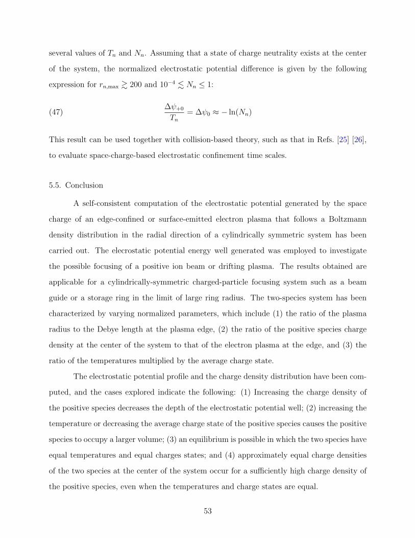
several values of Tn and Nn. Assuming that a state of charge neutrality exists at the center
of the system, the normalized electrostatic potential difference is given by the following
expression for rn,max & 200 and 10−4 . Nn ≤ 1:
(47)∆ψ+0
Tn= ∆ψ0 ≈ − ln(Nn)
This result can be used together with collision-based theory, such as that in Refs. [25] [26],
to evaluate space-charge-based electrostatic confinement time scales.
5.5. Conclusion
A self-consistent computation of the electrostatic potential generated by the space
charge of an edge-confined or surface-emitted electron plasma that follows a Boltzmann
density distribution in the radial direction of a cylindrically symmetric system has been
carried out. The elecrostatic potential energy well generated was employed to investigate
the possible focusing of a positive ion beam or drifting plasma. The results obtained are
applicable for a cylindrically-symmetric charged-particle focusing system such as a beam
guide or a storage ring in the limit of large ring radius. The two-species system has been
characterized by varying normalized parameters, which include (1) the ratio of the plasma
radius to the Debye length at the plasma edge, (2) the ratio of the positive species charge
density at the center of the system to that of the electron plasma at the edge, and (3) the
ratio of the temperatures multiplied by the average charge state.
The electrostatic potential profile and the charge density distribution have been com-
puted, and the cases explored indicate the following: (1) Increasing the charge density of
the positive species decreases the depth of the electrostatic potential well; (2) increasing the
temperature or decreasing the average charge state of the positive species causes the positive
species to occupy a larger volume; (3) an equilibrium is possible in which the two species have
equal temperatures and equal charges states; and (4) approximately equal charge densities
of the two species at the center of the system occur for a sufficiently high charge density of
the positive species, even when the temperatures and charge states are equal.
53

The electrostatic potential well depth has been evaluated for the two-species system.
It has been found that, once the positive species is introduced, the electrostatic potential
well depth reaches a saturation regime when the normalized size is sufficiently large. The
electrostatic potential well depth has been described analytically in this saturated regime.
the results obtained can be applied to evaluate space-charge-based electrostatic confinement
time scales. The concept could be of particular utility for investigation of atomic or molecular
processes in plasmas.
54

CHAPTER 6
ELECTRON BEAM TRANSMISSION THROUGH A CYLINDRICALLY SYMMETRIC
ARTIFICIALLY STRUCTURED BOUNDARY
6.1. Introduction
Experimental research on charged particle confinement and control by an electro-
magneto-static field configuration created by a cylindrically symmetric artificially structured
boundary (ASB) is presented. The ASB produces a periodic set of magnetic field cusps that
are plugged electrostatically. In the trapping system presented, the reflection or modification
of charged particle trajectories occurs near the confining boundary where the confining fields
have a relatively high strength. Away from the boundary, an essentially field free region
exists where confined particles are expected to reside. A field-free confinement region is
highly desired as a prospecting tool for experiments with particle trapping, particle-particle
interaction, particle-external field interaction, and self-consistent relaxation of plasmas.
The system presented here has several potential applications in electron or ion beam
physics and plasma physics such as in ion sources, ion or electron beam guides, and as
a charged particle trap. A cylindrically symmetric experimental apparatus has been con-
structed and its description is given. The characteristics of beam acceptance and transmis-
sion for the system operated as a beam guide are presented.
6.2. Apparatus
The components of the experimental apparatus are an electron source, a charged
particle trap or beam guide, and charged particle detection system. The electron source
consists of an electron gun and an electrostatic einzel lens that focuses the electron beam
at the trap entrance. The charged particle trap consists of a cylindrically symmetric ASB
configuration. This configuration produces spatially periodic electro- magneto-static fields
for the confinement of charged particle trajectories. Charged particles that leave the trap
through the exit side are detected with a position- and (relative) intensity-sensitive charged
particle detection system. An Ultra-High-Vacuum (UHV) chamber houses the electron gun,
55

Camera
Einzel LensElectron Gun
Entrance Electrode Exit Electrode
MCP
Phosphor ScreenVacuumPermanent Ring Magnets
OFHC Copper Electrodes
EntranceFaraday Cup
Exit Cup
Figure 6.1. Schematic view of experimental apparatus.
the charged particle trap, and the detection system. Figure 6.1 is a schematic representa-
tion of the experimental apparatus. The experimental hardware and software developed to
operate the apparatus as a charged particle trap is shown in Appendix D.
6.3. Electron Beam
The source of electrons is a Kimball Physics Incorporated (KPI) electron flood gun
(EFG-8) and electron gun power supply (EGPS-8) capable of supplying an electron beam
from a few eV to 1.5 keV with an energy spread of less than 0.4 eV and an emission current
of up to hundreds of µA, as per manufacturer specifications. The einzel lens assembly
was custom designed to focus charged particles on the center of the entrance to the trap.
Space limitations constrained the dimensions of the einzel lens but were optimized through
simulation. The einzel lens was simulated in SimIon [35] to determine the dimensions of
the lens elements which would allow focusing, in decelerating mode, of charged particles
before or after the center of the entrance electrode. The einzel lens elements are made of
oxygen-free high conductivity (OFHC) copper and, when assembled, are isolated from each
other by ceramic balls (D = 0.317 cm), which also serve to align the lens elements.
Refer to Fig. 6.1: For an electron beam with an energy of 30 eV, the voltage biasing
the center einzel lens element was varied to optimize empirically electron beam current at
the entrance of the trap, as measured by the entrance Faraday cup. This procedure was
carried out both with the experimental system and in the SimIon simulation environment.
56

The results are shown in Fig. 6.2. The procedure to obtain the plotted points from the
electron gun-einzel lens simulation is as follows. A simulation environment was created in
SimIon with the dimensions of the electron gun-einzel assembly. A classical trajectory Monte
Carlo simulation was carried out in SimIon where the electrons originated uniformly from a
1 mm disc into a velocity cone with half-angle α = tan−1(v⊥v‖
)= 15o. Here v‖ and v⊥ are the
components of the velocity vector parallel and perpendicular to the axis of the cylindrically
symmetric system simulated, respectively. 5,000 trajectories were simulated to obtain each
plotted point in Fig. 6.2. For each simulated charged particle trajectory, the position and
velocity vectors were recorded when the simulated trajectory terminated at the boundary
of the volume or at the surface of any of the electrodes in the simulation. The simulated
charged particle trajectories that terminated at an electrode that represented the entrance
Faraday cup were summed. The values thus obtained are plotted as Nn,i = NiNmax
in Fig. 6.2,
where Nmax = 3472 is the value with the einzel biased to −24 V (decelerating mode). The
plot shows the magnitude of the bias voltage as the abscissa. The SimIon simulation of
the electron gun-einzel lens-Faraday cup system can be used to determine the parameters
necessary to focus electrons or ions with different energies and other initial conditions.
An experiment was performed where the electron current on the entrance Faraday cup
was recorded as a function of einzel biasing voltage. Inside the gun, electron emission occurs
by heating of an yttria coated (Y2O3) disc of 1 mm in diameter. The gun construction limits
the emission to 11o , when ballistic trajectories are assumed, via a collimating aperture. The
entrance Faraday cup in the experimental setup was biased to 27 V to suppress secondary
electron current. The corresponding electrode in the simulation was also set to 27 V. The
plotted points in Fig. 6.2 which correspond to the recorded current on the Faraday cup were
normalized with respect to the maximum current observed; Imax = −63.5 nA, which occurred
at an einzel biasing voltage of −24 V. The plotted points are In,i = IiImax
, a quantity that is
proportional to the number of electrons incident on the Faraday cup per unit time. During
experimentation, the electron gun was set in electronic current control (ECC) mode, which
kept the current nearly constant over several hours after conditioning for 30 min. The current
57

• • • • • • • • ••
• • ••
•
••
•
´´
´´ ´ ´
´
´´´´
´´
´´
´
Experiment H •L = In,i
SimulationH ´ L = Nn,i
0 5 10 15 20 25 300.0
0.2
0.4
0.6
0.8
1.0
V
Num
bero
fPar
ticles
HNor
mali
zedL
Figure 6.2. Relative number of particles incident at the entrance of the trap
as a function of the magnitude of einzel lens focusing voltage. The einzel lens
was biased to provide focusing in decelerating mode. 5,000 electron trajectories
were simulated per data point marked by a cross. The maximum number of
electron trajectories that collapsed onto the Faraday cup electrode was 3472,
occurring at an einzel bias voltage of −24 V. Data points marked by dots are
the electron currents observed at the Faraday cup in the experimental setup,
normalized to the maximum current of −63.5 nA observed for an einzel lens
bias of −24 V.
was measured for less than 1 h to produce all In,i data points. In Fig. 6.2, the current at the
entrance cup shows a broad maximum for einzel lens voltage of −22 V to −27 V. Given the
close agreement between the simulated and experimental points plotted in Fig. 6.2, electron
beam characteristics such as beam intensity and phase-space properties can be inferred from
the simulation with confidence.
6.4. Experimental Artificially Structured Boundary
The charged particle trap presented here is defined as a cylindrically symmetric vol-
ume that has its interior boundary surface lined by an ASB with electrostatic plugging. The
system has been constructed to explore its possible application as an ion source, as an ion
58

beam guide, or as an ion trap. The electro- magneto-static fields have been designed for
trapping charged particles and plasmas or for guiding ion or electron beams. An ASB that
creates a periodic set of magnetic field cusps has been predicted to reflect charged particles
of either sign of charge simultaneously. Reflection of charged particles occurs most effec-
tively when their trajectories have grazing angles of incidence [2]. An ASB with electrostatic
plugging to has been predicted to confine effectively a single species of charge [36]. The
behavior of an electron plasma and an argon plasma in the vicinity of a planar segment of an
ASB has been observed to be strongly governed by the shape of the magnetic fields [12, 9].
These considerations have been taken into account to develop the electric and magnetic
fields within the volume lined by the ASB described here. Figure 6.3 shows the magnetic
Plugging Electrodes Magnets
Ring Cusp Point Cusp Point Cusp
Equipotential Contours
Figure 6.3. A length-wise cross-sectional view of the cylindrically symmetric
ASB and the fields produced within its interior. The rectangular features on
the top and bottom figures are the magnets and electrodes that create the
ASB. The lines in the top figure show contours of equal electric potential. The
lines on the bottom figure show the magnetic field. See text for further details.
59

field produced by a periodic set of ring magnets and a possible electrostatic biasing scheme.
The electrostatic field forms electrostatic mirrors axially at the entrance and exit of the trap.
The magnetic field forms magnetic mirrors. Charged particles can be confined in the axial
direction by either or both of these two fields. Charged particles are confined radially by the
magnetic fields near the magnet surfaces and by electrostatic barriers present at the location
of the magnetic field ring cusps.
A B
C
Figure 6.4. Photographs of the experimental system. Panel A shows the
alternating sequence of copper ring electrodes and permanent ring magnets.
Panel B shows the trapping volume as viewed upstream from the exit side.
Panel C shows the phosphor screen that, along with the micro-channel plates
(not shown), constitute the electron detection system.
Images of the actual system are shown in Fig. 6.4. The material structure consists of
a sequence of 12 neodymium-iron-boron high-strength permanent ring magnets (dimensions:
ID = 1.27 cm, OD = 2.54 cm, thickness = 0.254 cm) that alternate positions with 13 OFHC
copper ring electrodes (dimensions: ID = 1.78 cm, OD = 3.75 cm, thickness = 0.200 cm). The
60

magnets are arranged with like poles facing each other so that magnetic field ring cusps are
created between any two magnets. The magnets and electrodes are kept electrically isolated
from each other by mica washers (dimensions: ID = 1.90 cm, OD = 2.54 cm, thickness =
0.0254 cm). The magnet/electrode structure is electrically isolated from the entrance and
exit electrodes by ceramic balls (D = 0.317 cm). The spatial period of the magnetic field is
0.95 cm, with six full periods constituting the length of the trap. The distance from the center
of the entrance electrode to the center of the exit electrode is 7.62 cm, and from the center
of the exit electrode to the front face of the first MCP is 0.64 cm. The maximum magnetic
field at the surface of the magnets is specified by the manufacturer to be 0.3 T. A maximum
magnetic field of ≈ 0.2 T was measured before assembling the structure. A simulation of the
magnetic fields was developed in Vizimag [37] in order to observe the magnetic fields with
in the trap. In the simulation, a maximum magnetic field strength of 0.3 T was used along
with scaling set to represent the physical dimensions of the magnets and the assembly itself.
The resulting simulated magnetic field is shown in Fig. 6.3. The magnitude of the magnetic
field in the middle of the central ring cusp is approximately 0.08 T, and 0.017 T at the center
of the axial point cusps. Reflection or confinement of charged particles by the magnetic
field of an ASB has been predicted, see for example [36], to occur when the Larmor radius
is significantly smaller than the spatial period of the fields. The magnets are nickel plated
and are connected in three groups of four magnets each; one inner and two outer groups.
The electrodes are connected in three groups with three electrodes in the inner group and
five electrodes in each of the outer groups. In this manner, different biasing schemes can be
explored for diagnostic purposes.
6.5. UHV Conditions During Experimentation
The vacuum chamber is evacuated from atmospheric pressure to a base pressure of
5× 10⁻⁹ Torr in four stages: 1) A dual sorption pump stage achieves a vacuum of 100 mTorr
with the first sorption pump and ≈ 20 mTorr with the second one. 2) A turbomolecular
pump, backed by a rotary vane pump, takes over and evacuates the chamber until the ion
pump can be started, typically at 10−6 Torr. 3) Once the ion pump starts, the vacuum
61

Figure 6.5. Phosphor screen as imaged by SBIG ST-7XMEI SBIG CCD
camera (left panel). An electron beam exiting the trap and incident on the
MCP/Phosphor assembly creates the time integrated fluorescence recorded by
the CCD camera (right panel). For reference, the phosphor screen (major
circular feature on left panel) is 1.9 cm in diameter (or ≈ 500 pixels; 1 pixel
unit (pu) = 38µm). The same scale applies to right panel.
chamber is isolated from the previous two pumping stages by a gold seal valve. The ion
pump keeps the system at ≈ 5 × 10⁻⁹ Torr. 4) The last pumping stage is composed of a
titanium sublimation pump and a getter pump with a cryostat cooled by liquid nitrogen.
The last stage is typically turned on only during an experiment and nominally achieves
a vacuum better than 5 × 10⁻¹⁰ Torr. Particular care was taken to choose materials and
cleaning practices compatible with UHV conditions. The ring magnets that generate the
magnetic fields and the mica spacers are expected to be the main factors that limit the base
pressure of the vacuum system from achieving a lower value.
6.6. Electron Detection System
An electron detection system has been fitted to the exit side of the trap, and is
electrically isolated from the exit electrode (and to every other element on the system)
by ceramic balls that serve also as spacers. The electron detection system consists of a
Chevron pair of micro-channel plates (MCPs) that are biased so that the input side of the
62

first MCP is at +500 V with respect to ground and there is an 1800 V difference across the
MCP assembly. The electron cascades produced by the MCPs when electrons are incident
on the MCP assembly produce light when they impinge on a (P-22 Blue) phosphor screen
held in a metal cage structure biased at +2.8 kV with respect to ground. Activity occurring
on the phosphor screen is recorded using an ST-7XMEI SBIG CCD camera located outside
the vacuum chamber. Figure 6.5 (left panel) shows the phosphor screen when the vacuum
chamber is illuminated by an external light source and the image is recorded by the CCD
camera. Figure 6.5 (right panel) shows the emission from the phosphor screen as captured
by the CCD camera when the phosphor emission, due to the MCP electron cascade, is
the predominant source of light. The actual size of the phosphor screen is 1.91 cm, which
corresponds to the main circular shape in Fig. 6.5 (left panel) that covers ≈ 500 pu (pu =
pixel units).
6.7. Accepance and Transmission Without Electrostatic Plugging
The characteristics of electron beam transmission through the cylindrically symmetric
volume that has its interior lined with an ASB are now presented. The experimental results
obtained in this section show the dependence of a transmitted electron beam on input pa-
rameters. In this experiment, an electron beam was incident at the entrance to the trap,
and a portion of the beam was transmitted through the trap. The exiting electrons, and
their locations were detected and recorded by the MCP-phosphor screen and CCD camera
detection system. Relative beam intensity as a function of position could be deduced from
the magnitudes of the pixel values in the recorded images.
A 30 eV electron beam with a steady beam current of −63.5 nA was incident on the
entrance side of the structure. The electron beam focal point was varied by changing the
einzel lens voltage so that a diverging, focused, and over-focused beam was incident at the
entrance point cusp. Electron beam acceptance into the structure, as a function of einzel lens
voltage, is shown in Fig. 6.6. The ring electrodes were virtually grounded through a current
integrator and the ring magnets grounded through an ammeter. In Fig. 6.6, the normalized
integrated current (normalized with respect to the maximum value observed of 6 nC in 180 s
63

•••
•
•••
•
••
•••••••
••
´´
´
´
´´
´
´
´´´´´´´
´
IntegratedCurrent on Ring Electrodes H•LIntegratedTransmittedBeam Intensity H ´ L
0 5 10 15 20 25 300.0
0.2
0.4
0.6
0.8
1.0
1.2
V
Num
bero
fPar
ticles
HNorm
alize
dL
Charge on HUnbiasedL PluggingElectrodes
Figure 6.6. Electron beam acceptance into the trap as a function of einzel
lens voltage. Data points marked by dots are the normalized charge collected
on the unbiased plugging electrodes. Data points marked by crosses are the
time and space integrated relative beam intensities obtained by processing the
images recorded with the CCD camera. See text for details.
at −24 V einzel voltage) that reached the grounded ring electrodes is plotted as a function of
einzel lens voltage. The integrated current is directly proportional to the number of electrons
hitting the ring electrodes but is not equal to the total number of electrons collapsing onto
the electrode since secondary electron suppression was not employed. Secondary electron
emission can be suppressed by biasing the electrodes positive but electrons within the trap
would also be accelerated toward the ring electrodes. The secondary electron emission from
copper due to a 30 eV electron beam has been shown to be a constant fraction of the electron
current striking the copper surface. The effect that biasing the ring electrodes may have on
electron beam transmission is not considered here.
Also plotted in Fig. 6.6 is the time integrated beam intensity exiting the trap as
acquired by the CCD camera with an exposure time of 180 s. The image obtained from the
64

Figure 6.7. Spatial electron beam profile distribution as a function of focus-
ing at the entrance to the trap. The three dimensional shape that protrudes
from the x-y plane in the z direction is a plot of intensity I(in arbitrary units
(au)) as a function of position. The bands represent equal fractional intervals
of the peak intensity in each of the panels. A contour plot is also shown at the
top of each figure to illustrate the 2D beam profile. The data processed for
the plots shown are the pixel values that represent the images of the beam as
captured from the phosphor screen by the CCD camera. An example of such
an image is shown in the right panel of Fig. 6.5. The x and y coordinates are
in pixel size units (pu).
65

camera for each einzel setting was converted to a 2D array of values, where each value in the
array corresponds to a recorded value of a pixel in the image. The values of the array which
corresponded to a circular region containing the beam spot were summed to yield a single
value representing the integrated beam intensity. These values are normalized to the peak
value of the integrated intensity and are shown by a crosses in Fig. 6.6.
The number of electrons that reach the ring electrodes is observed to peak when the
einzel lens focusing voltage is −24 V. With this observation, and with the assumption that
the number of electrons reaching the ring electrodes is proportional to the number of electrons
that enter the trap, the maximum number of electrons that enter the trap occurs at an einzel
lens voltage of −24 V. The number of electrons incident on the electron detection system is
also observed to peak at the same einzel lens focusing voltage. However, notice that although
the plots in Fig. 6.2 and Fig. 6.6 peak at the same value of the einzel focusing voltage, Fig. 6.6
peaks more sharply. The decrease in intensity away from the maximum admitted number
of particles is attributed in part to a loss of unfocused electrons on apertures upstream of
the ring electrodes (same as the cause of the peak observed in 6.2), and additionally to a
portion of the electrons in the beam not meeting the phase space requirements to penetrate
the magnetic point cusp at the entrance to the trap (see Appendix C).
The results presented here pertain only to a 30 eV electron beam. There were two
reasons for choosing such an energy: (1) The electron gun can supply a steady current at this
energy; it is more stable when operating near the middle of its emission current and energy
range. (2) 30 eV electron trajectories within the trap have been predicted to be confined by
the magnetic field inside the trap [36]. For 30 eV electrons in this apparatus, the maximum
Larmor radius possible is 1 mm at the center of either point cusp and 250µm at the center
of a ring cusp, in the region between two magnets. An electron will be confined radially
within the trap if its Larmor radius at the center of the ring cusp is smaller than the spatial
period of the magnetic field by at least a factor of five, a condition that is clearly met by
30 eV electrons.
66

Information regarding electron beam characteristics upon exiting the trap was ob-
tained by processing the images acquired with the CCD camera; see an image example in
Fig.6.5 (right panel). The detection system is position sensitive to within a few MCP-channel
pores (diameter 25µm), and intensity sensitive to one part in 65536 (a digitized dynamic
range of 16 bits), where a pixel value of zero corresponds to a dark pixel and 65536 corre-
sponds to a bright saturated pixel. The pixel values are directly proportional to the number
of electrons incident on the MCP assembly at a given location. As a result, the transmitted
beam shape and intensity can be obtained as a function of electron beam parameters at the
entrance to the trap. The integrated beam intensity exiting the trap is shown in Fig. 6.6.
In Fig. 6.7, the relative spatial intensity distribution of the exiting beam is shown as
a function of einzel lens focusing voltage. The relative intensity is shown by the 3D shape
that protrudes from the x-y plane toward the positive z-axis. A cross-section of the beam
profile is shown by the contour plot included at the top of each figure panel. In each of these
figures, the intensity was normalized to the peak intensity of the profile measured for an einzel
voltage of −24 V, with electrostatic plugging turned off (ring electrodes grounded through
the current integrator, magnets grounded through ammeter, entrance and exit electrodes
directly connected to ground). To produce the plots shown in Fig. 6.7, the images obtained
from the camera were processed in the following manner: (1) The image data were changed
to a 2D array of values that corresponded to pixel values and then cropped to a square region
sufficiently large to contain the beam spot. (2) All pixel values were normalized by the peak
pixel value found for the image that was obtained when the einzel voltage was set to −24 V.
(3) A surface plot was generated for each of these 2D arrays. Figure 6.7 shows the electron
beam intensity profile, in arbitrary units (I (au)) as a function of position (in pixel units
(pu)) obtained by such a procedure. The four panels shown correspond to an over-focused
(einzel voltage = −26 V), optimally focused (einzel voltage = −24 V), and under-focused
(einzel voltage = −22 V and einzel voltage = −20 V) electron beam at the entrance to the
trap.
67

The information obtained from the integrated intensity is a proportional measure of
the current density of the electron beam exiting the trap because (1) The data for each of
the figures was obtained by setting an exposure time to 180 s and (2) the cross sectional
area of the transmitted beam is nearly constant and independent of focusing or defocusing
at the entrance to the trap. The maximum electron beam current density exiting the trap
occurs when the electron beam is optimally focused at the entrance to the trap. Focusing
or defocusing does not affect the size of the transmitted beam; only the transmitted beam
intensity is affected. To help show this, the full range of pixel values for each of the panels in
Fig. 6.7 was divided into ten intervals of equal magnitude, represented by alternating blue
and orange bands along the z direction in the figure. The highest point of each of these
shapes represents the most probable location where electrons exit the trap. The alternating
bands represent cylindrical bins, each of which has a 10% lower pixel value, as compared to
the maximum value, than the one above it. In the panel for einzel voltage of −24 V, the
value of the pixel at the top is unity (with all other values in Fig. 6.7 normalized with respect
to this value). The highest pixel value that corresponds to an einzel lens voltage of −22 V is
about half the pixel value that corresponds to the einzel lens voltage of −24 V. In this case,
the top most band covers a range of pixel values from 0.5 to 0.45, the next band from 0.45
to 0.40 and so on.
The contour plot at the top of each panel is a projection of the 3D figure onto the
top plane (top view) where the contours correspond to the inner and outer radii of the
corresponding bands in the 3D figure. These contour plots show that the beam size is
essentially constant with a beam diameter of ≈ 100 pu or 3.8 mm. The characteristics of
the beam incident at the entrance to the trap, as determined by the einzel setting, are not
present at the exit side. These observations lead to the conclusion that the beam profile is
governed by the shape of the fields present within the trap and by the shape of the magnetic
field at the exit point cusp and not by the ion-optical elements before the trap. The beam
waist size and cross-sectional profile are essentially constant, independent of focusing at
the entrance to the trap. However, the intensity of the electron beam observed exiting the
68

trap is dependent on the focusing at the entrance to the trap. The optimal electron beam
acceptance conditions manifest as the maximum electron beam current density at the exit
side of the trap. A similar behavior is expected for higher energy electrons, or ions, as long
as the fields are scaled accordingly.
6.8. Summary and Conclusion
A cylindrically symmetric system that employs an Artificially Structured Boundary
(ASB) to produce electro- magneto-static fields for charged particle confinement and control
has been presented. Electron beam transmission through the experimental apparatus con-
structed shows that electron trajectories through the trap are primarily controlled by the
magnetic field at the entrance to, inside of, and at the exit of the trap. The beam spot size
was observed to not change for a range of electron beam focusing conditions at the entrance
to the trap. For 30 eV electrons incident at the entrance to the trap, optimized transmission
manifests as a high intensity beam exiting the trap. A similar behavior is expected for other
ions or other energies as long as the fields are scaled appropriately. The results presented
show that this system could potentially be employed as a charged particle beam guide or ion
source.
69

CHAPTER 7
CONCLUSION
A system capable of modifying charged particle trajectories of either sign of charge
has been presented. Such a system consists of an ASB which generates periodic magnetic
field cusps that are plugged by electrostatic potential energy barriers. A segment of a planar
ASB was shown to reflect charged particles of either sign of charge when the appropriate
potential energy barrier was activated. A system that employs nested potential energy bar-
riers along the magnetic field cusp, where the magnetic field is nearly constant, has been
predicted to confine charged particles of either sign of charge simultaneously. A sequence of
current carrying wires, which alternate in the sign of current carried, could be employed to
generate the magnetic field cusps that could be electrostatically plugged by a nested config-
uration of potential energy barriers. The system experimentally studied employs permanent
magnets, which are stacked with like poles facing each other to generate a periodic sequence
of magnetic field cusps. Due to the shape and length of the magnetic field cusps generated
by such an arrangement of permanent magnets, only a single potential energy barrier can be
applied. Activation of the electrostatic potential energy barrier had a significant effect on
charged particle trajectories when these penetrated the ASB through a magnetic field cusp.
Neither the extent to which the activation of the potential energy barrier reflected charged
particle trajectories nor the actual behavior of charged particles in the region of where a
potential energy barrier overlaps with the magnetic field cusp could be determined from the
experimental system built.
A computer simulation was created to determine such behavior and to quantify the
capabilities of an ASB to reflect charged particle trajectories when a single potential energy
barrier is present along the magnetic field cusp. This simulation showed that a single species
of charge can be confined very effectively when the magnetic and electric fields generated have
moderate strengths as compared to the average energy of the charged particles in question.
Due to the short range of the fields generated by an ASB, it had been suggested that a
70
volume which has its interior surface composed of an ASB could provide a field-free region in
which charged particles or plasmas could be confined. Additionally, a single species plasma
would relax, due to self fields, within such volume. A study was carried out where the self-
consistent relaxation of an edge-confined plasma was computed assuming that such a plasma
follows a Boltzmann distribution. Deep potential energy wells are thereby predicted to occur
a the center of such an edge-confined and self-consistently relaxed plasma. An example of
an edge-confined plasma would be an electron plasma that relaxes within the a volume lined
by an ASB. Consequently, the potential energy well created by the space charge of the edge
confined plasma could be used to confine a plasma species which is oppositely charged. In
this manner, simultaneous confinement of charged particles of either sign of charge has been
predicted to occur.
An experimental system was built in which a cylindrically symmetric volume has
the interior surface lined by an ASB. Such a system has potential applications as an ion
source, ion beam guide, and as a charged particle trap. Results that pertain to electron
beam transmission were presented.
71

APPENDIX A
NORMALIZATION OF MAXWELLIAN DISTRIBUTION
72

Consider a Maxwellian source of charged particles with an associated temperature T ,
which has units of energy. The Maxwellian velocity distribution normalized to unity reads
(48) f(v) =( m
2πT
) 32e−
mv2
2T ,
where |v| = v, and v2 = v2x + v2
y + v2z . The Maxwellian distribution for each dimension is
separable and can be written as
(49) g(vi) =( m
2πT
) 12e−
mv2i2T ,
with i = x, y, z. The first moment (the average of a Cartesian velocity component) of the
Maxwellian distribution is of course zero, but the second moment is
(50) v2 =
∫v2f(v)d3v =
3
mT.
Equivalently,
(51)1
2mv2 =
3
2T,
which is the average kinetic energy of a particle in a system of particles that follows a
Maxwellian distribution. This is the amount of energy with respect to which the system is
normalized in Chapter 3.
Random variables with normal distributions can be used to construct an initial ran-
dom velocity vector from a Maxwellian distribution [13]. A distribution of the form
(52) f(Xi) =1√2πe−
X2i2
is adequately sampled by the random variable Xi
(53) Xi = (−2 log[R1i])1/2 cos(2πR2i),
73

where Rji are independent random numbers in the range (0, 1) sampled from a uniform
distribution [14]. From Eq. (49), define
(54) fn(vi) = g(vi)
√T
m=
1√2πe−
12 [√
mTvi]
2
so that, by inspection of Eqs. (53) and (52), the random components of velocity sampled
from a Maxwellian distribution are
(55) vi =
√T
m(−2 log[R1i])
1/2 cos(2πR2i).
Equation (55) is used to sample the initial conditions for the velocity vector in Sec. 3.2.
74

APPENDIX B
PRODUCT LOGARITHM
75

Here is given a derivation of the functional behavior of the electrostatic potential
well generated by an edge confined plasma. This approximation applies for systems that are
> 100 Debye lengths in size.
Spherical symmetry
Assume a plasma sphere with radius rp that is confined by a spherical boundary with
a radius rw. Next, the electric fields at rp and at rw are found for a spherically symmetric
system; see Fig. B.1. Use Gauss’s law:
(56)
∮E · dA =
Qencl
ε0,
where E is the electric field, A the surface area that encloses the region of interest and has
a normal vector pointing radially outward, ε0 the permittivity of free space, and Qencl the
enclosed charge. The total enclosed charge is
(57) Qencl =
∫ rp
0
qn(r)dΩr2dr = 4πq
∫ rp
0
n(r)r2dr.
Notice that for a system of 100 Debye lengths, the number density n(r) ≈ n0; see Sec. 4.2.
Making this approximation, the charge enclosed is approximately
(58) Qencl =4
3πqn0r
3p,
so that the electric field at the edge of the plasma becomes
(59) Ep4πr2p =
4
3ε0πqn0r
3p → Ep =
Ze
3ε0n0rp
where q = Ze has been substituted.
At the wall that confines the plasma, rw > rp, and the electric field there is obtained
via
(60)
∮Ew · dA =
Qencl
ε0,
76

(64) Qencl =
∫ rp
0
qn(r)dφdzrdr = 2πqL
∫ rp
0
n(r)rdr
where L is the length of the cylindrical boundary. For a system of 100 Debye lengths in size,
n(r) ≈ n0; therefore
(65) Qencl = Lπqn0r2p.
The electric field at the edge of the plasma becomes
(66) Ep =Ze
2ε0n0rp,
where q = Ze has been substituted.
At the wall where the plasma is confined, rw > rp, the electric field is obtained via
(67)
∮Ew · dA =
Qencl
ε0,
which yields
(68) Ew =Qencl
2πrwLε0=Zen0r
2p
2ε0rw
;
therefore,
(69) Ew = Ep
[rp
rw
]for cylindrical symmetry.
Planar symmetry
Assume a plasma planar sheet as described in Fig. B.1 (right panel). The plasma
sheet thickness is again assigned the varialbe rp and the location of the planar boundary is
at rw. Next, the electric fields at rp and at rw are found for such system:
(70)
∮E · dA =
Qencl
ε0, and
(71) Qencl =
∫ rp
0
qn(r)dr1dr2dr3 = qAn0rp
78

where A is the planar area considered. For a system of 100 Debye lengths n(r) ≈ n0, so that
the electric field at the edge of the plasma becomes
(72) Ep =Ze
ε0n0rp
where q = Ze has been substituted. At the wall where the plasma is confined, rw > rp, the
electric field there is
(73) Ew = Ep.
Electrostatic potential difference between the wall and the plasma center
Notice that the electric fields calculated for the three different geometries can be
written as
(74) Ew = Ep
[rp
rw
]α−1
where α = 1, 2, 3 for planar, cylindrical, spherical symmetry, respectively. Define ∆φ to be
the electrostatic potential difference between the wall and the center of the charge distribu-
tion. Using the electric field, the electrostatic potential can be calculated:
(75) ∆φ = −∫ rp
rw
Ewdr −∫ 0
rp
Epdr.
For the spherical geometry considered,
(76) ∆φ = Q3r2p
[3
2− 1
R
]where Q3 = Zen0
3ε0, and R = rp
rw. For the cylindrical geometry considered,
(77) ∆φ = Q2r2p
[1
2+ ln(R)
]where Q2 = Zen0
2ε0. For the planar system,
(78) ∆φ = Q1r2p
[R− 1
2
]where Q1 = Zen0
ε0. Defining βα as
79

βα =
R− 1
2: α = 1
ln(R) + 12
: α = 2
32− 1
R: α = 3
so that ∆φα applies to all three systems as
(79) ∆φα =Zen0
αε0r2
pβα.
Assume that n0 = nsexp[−ZeT
∆φ]. In such case, we can write
(80) ∆φα =Ze
αε0r2
pβαnse−ZeT
∆φα .
This equation can be normalized with Ze = q and q∆φT
= ∆ψ:
(81) ∆ψα =1
α
[q2nsTε0
]r2
pβαe−∆ψα .
The quantity in brackets is the squared inverse Debye length. Substituting the Debye length
and assuming that rp ≈ rw = rmax, which is the case when the system is ≥ 100 Debye
lengths, then βα ≈ 12
and
(82) ∆ψα =1
2α
[rmax
λD
]2
e−∆ψα ,
where the quantity in brackets is now the maximum, normalized, system size rn,max. Making
that substitution and re-arranging the equation, we obtain
(83) ∆ψαe−∆ψα =
r2n,max
2α.
This equation has the form of the product logarithm (Lambert) function: Ξ = χexp[χ] ↔χ = W(Ξ), so that
(84) ∆ψα = W
(r2n,max
2α
).
The normalized electrostatic potential well depth is a function of the system size and the
geometry in question. Equation (26) was obtained by subtracting the product logarithm
80

function W(Ξ) from the self-consistent evaluation of ∆ψα; the resulting values were fit-
ted with a non-linear regression algorithm which yielded the best fit to be of the form:
ln[(rn,max)0.217α0.139
].
81

APPENDIX C
TRAPPING FIELDS, PARTICLE BEHAVIOR, AND PLASMA BEHAVIOR
82

Trajectories that Escape Through a Cusp
Acceptance of charged particle trajectories is in part governed by direction or charged
particle trajectories relative to the direction the magnetic field, and by the relative magnetic
field strength between the point where the trajectory starts and the center of the magnetic
field cusp. T. J. Dolan [38] presented the following derivation as applied to charged particle
trajectories near the point cusps of a magnetic mirror configuration assuming that only
adiabatic processes take place. Derivation that is equally applicable to point, ring, and line
cusps.
Assuming that charged particles that are electro- magneto- statically trapped expe-
rience only adiabatic processes, then the energy conservation equation becomes:
(85) E = (1/2)mv2‖ + (1/2)mv2
⊥ + qφ = (1/2)mv2‖ + µB + qφ = constant
where q and m are the test particle’s charge and mass, respectively, µ = mv2⊥/2B is its
magnetic moment and φ is the electrostatic potential. The components of the velocity
vector, v‖ and v⊥, are defined with respect to the direction of the magnetic field line at the
instantaneous location of the particle. When the trajectory of the particle and the magnetic
field are co-linear, then:
(86) (1/2)mv2‖ = E − µB − qφ
which shows that the particle can be stopped either magnetically or electrically. In the
presence of a magnetic field only (i.e, φ = 0) the particle will momentarily stop if
(87) µB = E.
83

As initial conditions, suppose that the particle starts with a velocity v0 in a region of zero
electrostatic potential and magnetic field with magnitude B0; when that is the case, then
(88) E − (1/2)mv2‖0 = µB0 = (1/2)mv2
⊥0,
and
(89) µ = mv2⊥0/2B0
since
(90) E = (1/2)mv20.
Substituting Eq. (89) and Eq. (90) back into Eq. (87), and rearranging gives
(91) B/B0 = v20/v
2⊥0 = 1/sin2α0
where α0 is the included angle between the direction of the magnetic field and the velocity
vector v0 and defines the upper limit on the largest angle that will penetrate the magnetic
field cusp. This angle is typically called the pitch angle in the literature related to magnetic
mirrors. This pitch angle places a constraint on the charged particles that enter or exit the
charged particle trap through the point cusps located at the axial ends. The charged particle
trap is described in Chapter 6.
An additional force to consider is
(92) F = −µ∇B
which acts to accelerate particles, positive or negative, in the direction of decreasing B. This
force can be a significant contribution to the modification of charged particle trajectories
where the magnetic fields change abruptly. Systems in which the magnetic field lines are
everywhere convex toward the location of the confined plasma are known to have Magneto-
Hydro-Dynamic (MHD) stability [39].
84

Charged Particle Motion
Charged particle motion within the trap is expected to be complex, especially when
the trapped entity is described as a plasma [34]. A qualitative description of the motion and
the general behavior of single particles within the trap is now given; Fig. C.1 is included here
for reference. At the center of the trap, both electric and magnetic fields are essentially zero
and charged particle trajectories are thus unaffected; only cold particles can reside there.
Due to the electrostatic fields, the motion in the axial direction is very similar to the motion
of charged particles in an electrostatic bottle or a harmonic trap [40]. However, the confining
magnetic field is periodic and non-uniform. Charged particles that travel radially and are
incident on the on the surface of the magnet experience a v ×B force that guides charged
particles in or out of the plane of the page. Once such trajectories have a velocity in the
azimuthal direction, these experience a v × B force that guides charged particles to the
center of the trap. Additionally, a ∇B force (see Eq. (92)), especially near the boundary,
has the effect of confining particles to the center of the trap, or focusing them at the location
of the magnetic field cusps. This effect of the ∇B force is the same for either sign of
charge and has a direction that points away from increasing magnetic field magnitude. It
is expected that the majority of charged particles that do enter the cusps are reflected back
toward the center of the trap. In the cusp, near the plugging electrode, charged particles can
experience an E×B force. However, this effect is expected to be small since the electric and
magnetic fields at the center of the electrode have nearly identical directions (but not so at
the center of the magnet!). Such an E ×B drift can have many effects, some of which are:
(1) generation of a constantly rotating layer, (2) migration back into the confining volume,
(3) enough energy gain that causes the particle to escape confinement. The first two are
desired, especially for space-charge-based confinement. With respect to the third of these,
particles that enter the magnetic field cusps are nearly parallel to the cusp and would fall
in the high energy tail of a Maxwellian speed distribution (see Sec. 3.3), a condition that
presents itself as a possible diagnostic tool. The probability of a charged particle escaping
through any one cusp is relatively low and proportional to the ratio of the total area of the
85

Plugging Electrodes Magnets
Ring Cusp Point Cusp Point Cusp
Equipotential Contours
Figure C.1. Cross-sectional view of an charged particle trap consisting of
overlapping electric and magnetic multipole fields. Trapping expected to occur
when both fields are physically superimposed.
ring cusps to the total lateral surface area of the trap, correlated with the energy distribution
of the trapped constituents; see Chapter 3. The point cusp fields at either end of the trap
very closely resemble magnetic mirrors and charged particles are also confined axially by this
effect, especially, and more strongly, when the trap is biased in such a configuration as to
create electrostatic mirrors along the axis.
Plasma Behavior.
Notice that the description given thus far deals only with the single particle limit.
When the trapped bunch of particles is described as a plasma, first and foremost, trapping is
limited by the density and temperature of the plasma. This is predicted to be a dominating
factor in plasma confinement as presented in Chapter ?? for an edge confined plasma and
for space-charge-based confinement, and dictated by the Debye length. A plasma with low
temperature and high density meets the ideal qualities for edge confined plasma and space
charged based plasma confinement.
86

An upper limit on the temperature is dictated by the electrostatic-plugging-potential
energy barrier of the ASB; see Chapter 3. An upper limit on the density is given by the
Brillouin limit. Such temperature and density can be used to define an edge confined plasma
where the actual experiment is expected to have an order of magnitude less on either parame-
ter. The energetic tail of the charged particle distribution will most likely escape confinement,
and although not desired, such an effect provides a potential plasma diagnostic tool and self
temperature regulation via evaporation. An equilibrium is thus expected for a range of tem-
perature and density conditions once a suitable temperature is reached. Plasma heating is
expected at the edge of the plasma, in the region of strong magnetic fields. However, periodic
counter rotations, due to the periodicity of the magnetic field, may mitigate such effect.
87

APPENDIX D
CHARGED PARTICLE TRAPPING
88

The electronic circuitry developed to operate the cylindrically symmetric ASB as a
charged particle trap is presented. A typical trapping cycle consists of (1) a narrow pulse of
charged particles that is injected into the trap, upon injection, (2) the entrance and exit gate
electrodes are biased to reflect and confine the charged particles for a preset time period,
and (3) the exit electrode is grounded so that trapped charged particles exit the trap and
are detected. The details regarding the equipment employed, software developed, and fast
timing circuitry to drive charged particle trapping cycle is shown.
Equipment
The fast timing circuitry developed to drive a the laboratory equipment for trapping
cycle is shown in Fig. D.2. A virtual instrument developed in LabView assigns the gate/delay
time intervals by programming two LeCroy dual gate generators (DGG, model 2323A) so
that a total of four gates/delays can be created to generate the pulses necessary for trapping.
The DGGs can be programmed manually or via LabView-GPIB-LeCroy 1434 crate interface
with a timing resolution of tenths of µs to few s with the possibility of delaying the output
Camera
Einzel LensElectron Gun
Entrance Electrode Exit Electrode
MCP
Phosphor ScreenVacuumPermanent Ring Magnets
OFHC Copper Electrodes
EntranceFaraday Cup
Exit Cup
Figure D.1. Trapping system description
89

for 10, 30, 100, 300ns as compared to the triggering signal. The gate/delay signals generated
by the DGGs have rise and fall times of < 50nc for all outputs (with matched impedances).
Each of the pulses used to trigger the pulsed power supplies is now explained as each
one is traced through the diagram shown in Fig. D.2. The transistor-transistor logic (TTL)
output from the DGG that starts the cycle triggers the opto-coupling circuit (Vishay High
Speed Optocoupler P/N 6N137). This circuit is triggered when a TTL signal is present at the
input side. With the correct pulse shaping circuit, a TTL pulse is present at the output side.
The output side of this circuit is can be electrically floating and is powered via a 1:1 isolation
transformer. An HP3310B function generator is also powered by the isolation transformer
and floating at −24 V with respect to ground. The nuclear instrumentation module (NIM)
pulse generated by this same DGG module is used to synchronize the timing between the
pulsed electron beam entering the trap and the entrance and exit gate electrodes. The width
of W1 is programmable and adjustable to lead, coincide with, or lag the leading edge of W1..
When the second module of the first DGG is triggered, a TTL pulse passes through
pulse shaping amplifier to provide the correct input for a Cober high power pulse generator
(605P). The width of W4 is programmable; the height of W4 is adjusted via a front panel
knob. The Cober pulse generator can provide a variable pulse height from 50 V to 2.2 kV
positive or negative with typical fall and rise times of < 30ns. W3 is created by a TTL pulse
that triggers an Instrument Research Co. (model 80S) pulsed power supply. The width and
height of W3 are set via front panel knobs. The Ins. Res. Co. pulse generator can provide a
negative variable pulse from −150 V to −350 V with rise and fall times of < 20ns. Matching
loading impedances is very important so that the power supplies can provide pulses with the
characteristics given.
Einzel lens bias and pulsed electron beam
In this system, the einzel lens focuses charged particles at the entrance of the trap
and, by pulsing the biasing voltage for the middle einzel lens element, the electron beam
is also pulsed. The einzel lens drive system is now described; see Fig. D.3. An HP3310B
function generator is electrically floating and negatively biased to a voltage, Vf , by a Kikusui
90

Einzel lens
Exit electrode
Entrance electrode
Ins. Res. Co. 80S
S
NIM
TTL
S
TTL
LeCroy 1434Dual Gate Gen.
2323A (1)
S
DLY
S
TTL
Dual Gate Gen. 2323A (2)
Pulse Amplifier
CoberHPPG605P
W4
Opto-CouplingCircuit
start
PC LabView
Floating Func.Gen.
HP3310B
W2
W1 synchronization of pulsed electron beam and gating electrodes
W3
Figure D.2. Experimental equipment for trapping charged particles with the
trap presented.
Electronics Corp. power supply. Such voltage is the optimal voltage for focusing an electron
beam with the einzel lens when in decelerating mode. For example, a 30 eV electron beam is
optimally focused, in the current system, when the einzel middle element is biased to −24 V;
see Fig. D.3. The pulse width and height are adjustable via front panel knobs. The function
generator pulse height is added to the focusing voltage and has a value of 0 V when triggered
and −9 V otherwise. In this manner, the beam is switched from being optimally focused at
the entrance to the trap to being off. The rise and fall times of the pulse generated by the
HP3310B are < 30ns. The function generator requires a TTL pulse for triggering, a fact that
poses a problem. This issue was resolved by using an opto-coupling circuit that activates a
light emitting diode by the leading edge of a TTL pulse coming from a LeCroy delay and gate
generator (2323A). The floating optical-detector side provides the appropriately referenced
signal to trigger the function generator. The DC-offset in the HP3310B function generator
is set so that the baseline is at −9 V and 0 V when triggered. The einzel lens voltage is thus
−33 V at baseline and −24 V when triggered, thereby achieving a pulsed and focused 30 eV
91

Trap
Einzel Lens Bias for Beam Pulsing.
Func. Gen. HP.
Vcc
Trigger
Vf
(W,H)
W
H
TTL
Entrance
Faraday CupEinzel LensElectron Gun
Gate/DelayGen.
LeCroy2323A
Opto-CouplingCircuit
Figure D.3. Einzel lens focusing and pulsed electron beam.
Pulse Sequence for One Trapping Cycle.
W1
W2
W3
delay
Wait
Load Dump
delay
Trapping Cylcle
Ins. Res. Co.
Cober
Floating Func. Gen. HP.
LabViewStart
Electron BeamON/OFF
Exit Gate
Entrance Gate W4
Time
Figure D.4. Time line of events to drive the trapping cycle.
electron beam at the entrance to the trap. A similar scheme is expected for other charged
particles and other energies.
92

Fast timing circuitry
Figure D.4 represents the event time line during a typical trapping cycle. In this
diagram, spikes are trigger signals to start the consequent delay or pulse. The horizontal
dashed lines indicate variable time intervals. Vertical dashed lines indicate the time at
which other events are triggered or stages during the trapping cycle. A driver was coded in
LabView which provides the initial trigger and repetition rate for the number of trapping
cycles desired. The initial trigger starts the first pulse, W1. The leading edge of W1 triggers
the electron beam ON. The delay between the trigger signal and electron beam pulse is
inherent to the circuitry necessary to switch the beam ON and OFF; see Fig. D.4. The
trailing edge of W1 triggers the biasing of the exit electrode to repel electrons. The leading
edge of W2 and W3 can be made to temporally coincide by varying the width of W1. The
flexibility is such that the leading edge of W3 can come before or after the leading edge
of W2. The correct overlap of W2 and W3 is dictated by the absence of signal at the
MCP/Phosphor screen electron detector. The trailing edge of W1 also triggers the biasing
of the entrance electrode to repel electrons. The delay between the trigger signal and the
leading edge of W4 is necessary to allow electrons to enter the trap and essentially defines the
time during which the trap is loaded with electrons. The signal transit time which produces
W4 is significantly longer than the signal transit time to generate W3. For this reason, W3
is delayed so that it nearly coincides in time with W4. Once W4 starts, the entrance to the
trap is blocked and no electrons enter the trap. The temporal overlap beteween W3 and W4
define the time during which charged particle trapping occurs. W2 is turned off after the
loading occurs but sufficiently long before the trailing edge of W4. The trailing edge of W3
marks the end of the trapping time, at which point charged particles can exit the trap and
be incident on the MCP/Phosphor screen detector. W4 is made sufficiently long to ensure
trap evacuation and maximize the events at the MCPs. During the dump time interval,
electrons are repelled from the entrance electrode and attracted by the fields present at the
exit due to the biasing of the MCPs. It is necessary that W4 stays ON for the remainder
of the trapping cycle but the duty cycle of the pulsed power supply limit this possibility.
93

Figure D.5. Front-end panel of virtual instrument (VI).
Additionally, the cycle repetition rate cannot be faster than the luminescence decay time of
the phosphor screen (≈ 25µs). In this manner, it is ensured that the source of electrons is
not ion-optically visible to the detector at any time; only electrons that could have become
trapped can be incident on the detection system.
Virtual instrument system driver
The basic components of the virtual instrument (VI) developed for the trapping cycle
are the front panel (Fig. D.5), block diagram of cycle driver (Fig. D.6), and block diagram to
program anyone DGG (Fig. D.7). In the front panel, the values of the delays and gates can
be adjusted by the user to change the pulse width or delay for the trapping cycle. The values
shown are those that would allow 1000 repetitions of a load-wait-dump cycle as specified in
the previous sections of this appendix.
94

Figure D.6. VI code segment that generates the start signal, cycle repetition
rate, and number of cycles.
95

Figure D.7. Typical VI code to program the anyone of the two modules in
a LeCroy 2323A DGG.
96

BIBLIOGRAPHY
[1] C. A. Ordonez, “Drifting plasma confinement with a spatially periodic field,” Plasma
Science, IEEE Transactions on, vol. 38, no. 3, pp. 388–392, 2010. 4
[2] C. A. Ordonez, “Charged particle reflection from an artificially structured boundary
that produces a spatially periodic magnetostatic field,” Journal of Applied Physics,
vol. 106, no. 2, 2009. 4, 11, 42, 59
[3] C. A. Ordonez, “Effect of a periodic electrostatic potential on magnetized particle trans-
port,” Physics of Plasmas, vol. 15, no. 11, p. 114507, 2008. 4, 23, 27
[4] T. J. Dolan, “Review article: Magnetic electrostatic plasma confinement,” Plasma
Physics and Controlled Fusion, vol. 36, pp. 1539–1593, 1994. 4
[5] C. A. Ordonez and D. L. Weathers, “Two-species mixing in a nested penning trap for
antihydrogen trapping,” Physics of Plasmas, vol. 15, no. 8, p. 083504, 2008. 4, 42
[6] M. Amoretti, C. Amsler, G. Bonomi, A. Bouchta, P. Bowe, C. Carraro, C. Cesar,
M. Charlton, M. Collier, M. Doser, V. Filippini, K. Fine, A. Fontana, M. Fujiwara,
R. Funakoshi, P. Genova, J. Hangst, R. Hayano, M. Holzscheiter, L. Jørgensen, V. Lago-
marsino, R. Landua, D. Lindelof, E. Lodi-Rizzini, M. Macri, N. Madsen, G. Manuzio,
M. Marchesotti, P. Montagna, H. Pruys, C. Regenfus, P. Riedler, J. Rochet, A. Rotondi,
G. Rouleau, G. Testera, A. Variola, T. Watson, and D. van der Werf, “Production and
detection of cold antihydrogen atoms,” Nature (London), vol. 468, pp. 673–676, October
2002. 4
[7] G. Gabrielse, N. S. Bowden, P. Oxley, A. Speck, C. H. Storry, J. N. Tan, M. Wessels,
D. Grzonka, W. Oelert, G. Schepers, T. Sefzick, J. Walz, H. Pittner, T. W. Hansch, and
E. A. Hessels, “Background-free observation of cold antihydrogen with field-ionization
analysis of its states,” Phys. Rev. Lett., vol. 89, p. 213401, Oct 2002. 4
[8] G. Andersen, M. Ashkezari, M. Baquero-Ruiz, W. Bertsche, P. Bowe, E. Butler, C. Ce-
sar, M. Charlton, A. Deller, S. Eriksson, J. Fajans, T. Friesen, M. Fujiwara, D. Gill,
A. Gutierrez, J. Hangst, W. Hardy, R. Hayano, R. Hayden, A. Humphries, R. Hydo-
mako, S. Josnell, S. Kemp, Kurchaninov, N. Madsen, S. Menary, P. Nolan, K. Olchanski,
97

A. Olin, A. Povilus, P. Pusa, F. Robicheaux, E. Sarid, S. Seif el Nasr, D. Silveira, C. So,
J. Storey, D. Thompson, R.I. van der Werf, J. Wurtele, and Y. Yamazaki, “Trapped
antihydrogen,” Nature (London), vol. 468, pp. 673–677, December 2010. 4
[9] J. L. Pacheco, C. Ordonez, and D. L. Weathers, “Plasma interaction with a static spa-
tially periodic electromagnetic field,” Plasma Science, IEEE Transactions on, vol. 39,
no. 11, pp. 2424–2425, 2011. 11, 23, 59
[10] J. L. Pacheco, C. A. Ordonex, and D. L. Weathers, “Electrostatic storage ring with
focusing provided by the space charge of an electron plasma,” in Application of Accel-
erators in Research and Industry, no. 1525, pp. 88–93, AIP Conference Proceedings,
2013. 11
[11] J. L. Pacheco, C. A. Ordonez, and D. L. Weathers, “Space-charge-based electrostatic
plasma confinement involving relaxed plasma species,” Physics of Plasmas, vol. 19,
no. 10, 2012. 12
[12] C. A. Ordonez and R. M. Hedlof, “Simulation of an aperture-based antihydrogen gravity
experiment,” AIP Advances, vol. 2, no. 1, p. 012176, 2012. 12, 23, 59
[13] C. A. Ordonez, W. D. Booth, R. Carrera, and M. E. Oakes, “Calculations of the sput-
tering energy reflection coefficient for hydrogen plasma ion bombardment on carbon
surfaces,” Radiation Effects and Defects in Solids, vol. 116, pp. 37–47, 1991. 16, 72
[14] G. E. Box and M. E. Muller, “A note on the generation of random normal deviates,”
Ann. Math. Stat., vol. 29, pp. 610–611, 1958. 16, 73
[15] W. H. Press, S. A. Teukolosky, W. T. Vetterling, and B. P. Flannery, Numerical Recipies:
The Art of Scientific Computing. Cambridge University Press, 2007. 17, 28, 46
[16] C. K. Birdsall and A. B. Langdon, Plasma Physics Via Computer Simulation. IoP, 1991.
17
[17] L. V. Jørgensen, “The aegis antihydrogen gravity experiment,” Hyperfine Interactions,
vol. 212, no. 1-3, pp. 41–49, 2012. 23
[18] C. A. Ordonez, “Effect of positron space charge on operation of an antihydrogen trap,”
Phys. Rev. E, vol. 76, p. 017402, Jul 2007. 23
98

[19] C. A. Ordonez, D. D. Dolliver, Y. Chang, and J. R. Correa, “Possibilities for achieving
antihydrogen recombination and trapping using a nested penning trap and a magnetic
well,” Physics of Plasmas, vol. 9, no. 8, pp. 3289–3302, 2002. 23
[20] M. E. Glinsky and T. M. O’Neil, “Guiding center atoms: Three-body recombination
in a strongly magnetized plasma,” Physics of Fluids B: Plasma Physics, vol. 3, no. 5,
pp. 1279–1293, 1991. 24
[21] C. A. Ordonez, “Fully and partially non-neutral plasma equilibria in a variable-
electrode-radius malmberg-penning trap,” Phys. Rev. E, vol. 67, pp. 046401–2, Apr
2003. 25
[22] R. L. Spencer, S. N. Rasband, and R. R. Vanfleet, “Numerical calculation of axisym-
metric nonneutral plasma equilibria,” Physics of Fluids B: Plasma Physics (1989-1993),
vol. 5, no. 12, 1993. 27, 28
[23] A. J. Peurrung and J. Fajans, “Non-neutral plasma shapes and edge profiles,” Physics
of Fluids B: Plasma Physics, vol. 2, no. 4, pp. 693–699, 1990. 28
[24] S. A. Prasad and T. M. O’Neil, “Finite length thermal equilibria of a pure electron
plasma column,” Physics of Fluids, vol. 22, no. 2, pp. 278–281, 1979. 28
[25] Y. Chang, J. R. Correa, and C. A. Ordonez, “Loss rate of an electrically trapped non-
neutral plasma,” Physics of Plasmas, vol. 11, no. 7, pp. 3360–3367, 2004. 35, 38, 51,
53
[26] J. R. Correa, Y. Chang, and C. A. Ordonez, “Collisional scattering for binary coulomb
interactions that are cut off at a distance different than the debye length,” Physics of
Plasmas, vol. 12, no. 8, p. 084505, 2005. 38, 53
[27] J. U. Andersen, P. Hvelplund, S. B. Nielsen, S. Tomita, H. Wahlgreen, S. P. Møller, U. V.
Pedersen, J. S. Forster, and T. J. D. Jørgensen, “The combination of an electrospray
ion source and an electrostatic storage ring for lifetime and spectroscopy experiments
on biomolecules,” Review of Scientific Instruments, vol. 73, no. 3, 2002. 42
[28] T. Tanabe, K. Chida, K. Noda, and I. Watanabe, “An electrostatic storage ring for
atomic and molecular science,” Nuclear Instruments and Methods in Physics Research
99

Section A: Accelerators, Spectrometers, Detectors and Associated Equipment, vol. 482,
no. 3, pp. 595 – 605, 2002. 42
[29] D. Zajfman, O. Heber, L. Vejby-Christensen, I. Ben-Itzhak, M. Rappaport, R. Fishman,
and M. Dahan, “Electrostatic bottle for long-time storage of fast ion beams,” Phys. Rev.
A, vol. 55, pp. R1577–R1580, Mar 1997. 42
[30] M. Dahan, R. Fishman, O. Heber, M. Rappaport, N. Alstein, D. Zajfman, and
W. van der Zande, “A new type of electrostatic ion trap for storage of fast ion beams,”
Rev. Sci. Instrum., vol. 69, pp. 76–83, January 1997. 42
[31] H. T. Schmidt, H. Cederquist, J. Jensen, and A. Fardi, “Conetrap: A compact elec-
trostatic ion trap,” Nuclear Instruments and Methods in Physics Research Section B:
Beam Interactions with Materials and Atoms, vol. 173, no. 4, pp. 523 – 527, 2001. 42
[32] Y. Ishida, M. Wada, and H. Wollnik, “A multi-reflection time-of-flight mass spectrom-
eter for mass measurements of short-lived nuclei,” Nuclear Instruments and Methods
in Physics Research Section B: Beam Interactions with Materials and Atoms, vol. 241,
no. 14, pp. 983 – 985, 2005. Proceedings of the Eighteenth International Conference on
the Application of Accelerators in Research and Industry (CAARI 2004). 42
[33] C. A. Ordonez, “Effective well of a static kingdon trap,” Physics of Plasmas, vol. 15,
no. 7, p. 072508, 2008. 42
[34] J. Fajans and A. Schmidt, “Malmberg penning and minimum-b trap compatibility:
the advantages of higher-order multipole traps,” Nuclear Instruments and Methods
in Physics Research Section A: Accelerators, Spectrometers, Detectors and Associated
Equipment, vol. 521, no. 23, pp. 318 – 325, 2004. 43, 82
[35] Idaho National Engineering and Environmental Laboratory. Ion and Electron Optics
Simulator. www.simion.com. 56
[36] J. L. Pacheco, C. A. Ordonez, and D. L. Weathers, “Artificially structured boundary
for a high purity ion trap or ion source,” Nuclear Instruments and Methods in Physics
Research B: Conferece Proceedings., Accepted, Publication Pending. 59, 61, 66
[37] J. S. Beeteson. Vizimag: Magnetic Field Simulator. www.vizimag.com. 61
100

[38] T. J. Dolan, Fusion Research: Principles, Experiments and Technology. Pergamon Press,
1982. 80
[39] J. Berkowitz, H. Grad, and H. Rubin, “Proceedings of the 2nd international conference
on peaceful uses of atomic energy,” vol. 1, (Geneva, Switzerland), pp. 177–189, 1958. 81
[40] T. Mohamed, H. Imao, N. Oshima, A. Mohri, and Y. Yamazaki, “Fast electron accu-
mulation and its mechanism in a harmonic trap under ultrahigh vacuum conditions,”
Physics of Plasmas, vol. 18, no. 3, p. 032507, 2011. 82
101