An Electrically Isolated UPS System with Surge Protection · PDF file ·...
63
COMPSYS 401A/B Part IV: Final Report An Electrically Isolated UPS System with Surge Protection Written By : Thusitha Mabotuwana (9790416) Department : Computer Systems – Department of Electrical and Computer Engineering Project Number : 57 Project Supervisor : Mr. Nihal Kularatna Second Supervisor: Dr. Patrick Hu Project Partner : Mr. Duleepa Thrimawithana (9778679) Date of Report : 13.09.2004
-
Upload
truonghanh -
Category
Documents
-
view
215 -
download
2
Transcript of An Electrically Isolated UPS System with Surge Protection · PDF file ·...

COMPSYS 401A/B
Part IV: Final Report
An Electrically Isolated UPS System with Surge Protection
Written By : Thusitha Mabotuwana (9790416) Department : Computer Systems – Department of Electrical and Computer Engineering Project Number : 57 Project Supervisor : Mr. Nihal Kularatna Second Supervisor: Dr. Patrick Hu Project Partner : Mr. Duleepa Thrimawithana (9778679) Date of Report : 13.09.2004

COMPSYS401A/B Thusitha Mabotuwana Part IV Project – Final Report 9790416
- Page i -
Summary
One of the main drawbacks of current Uninterrupted Power Supply (UPS) systems is their inability to fully protect user-applications from very high surges, such as those seen in tropical countries. Therefore the main aim of this project was to design a novel UPS system using self contained multiple energy storage elements to dynamically transfer energy while providing complete input-output isolation. Possibilities of using supercapacitors as the main energy storage elements of the system were also to be investigated. The complete system was to comply with the IEEE C62.41 Class B standard and provide common and differential mode surge protection. The final solution that has been implemented successfully transfers energy between the supply and load while providing complete input-output isolation, hence common and differential mode surge protection. Also possibilities of using supercapacitors for dynamic energy transfer have been investigated and proven to be feasible with experimental results. The implemented system consists of 4 main modules, an energy pump to provide DC, a charge transfer unit where three 0.2F/18V self-contained supercapacitor banks are cycled through charging-discharging-standby states to provide dynamic energy transfer and a single-stage push-pull sine modulated PWM inverter which converts the output of the charge transfer unit to an AC output. The last module is the Atmel Mega8535 microcontroller subsystem which provides control for the overall system. This report contains details of various design options that were considered for the above modules and experimental results obtained. In the final prototype that has been implemented a 15kHz, 40% duty cycle PWM scheme has been chosen as a suitable control mechanism for the energy pump and a 1kHz sine modulated PWM technique has been implemented to control the inverter with approximately 4% output voltage regulation. Algorithms and other timing issues pertaining to overall control are also discussed herein.

COMPSYS401A/B Thusitha Mabotuwana Part IV Project – Final Report 9790416
- Page ii -
Declaration of Originality
I declare that this report is my own unaided work and was not copied from or written in collaboration with any other person. Signed:_________________
(Thusitha Mabotuwana)

COMPSYS401A/B Thusitha Mabotuwana Part IV Project – Final Report 9790416
- Page iii -
Acknowledgement Researching for various aspects of the project and getting started was quite a daunting task for both, me and my partner Duleepa and I would like to take this opportunity to thank our supervisors Mr. Nihal Kularatna and Dr. Patrick Hu for all the support, encouragement and guidance given throughout. I would also like to thank my project partner Duleepa for being very supportive and helpful to me during the course of the project. It’s been a great privilege working with him and all his support and efforts are very much appreciated. Also special thanks to our technicians Mr. Grant Sargent for lending us tools and other equipment whenever required, Mr. Vic Church for providing us with electrical components and putting a lot of effort to get the PCBs ready in time, and Mr. Jerald Osborne for helping us gather various parts and products from the department store. The kind advice given to us throughout the project whenever required is also greatly valued. Finally I would like to thank my parents and all my dear friends, especially Kasun, Dilanka, David, Sasanka, Amal, Darshana, Punnaji and Harith for all the support given throughout the project and also giving useful feedback during the project poster and presentation preparation. Thusitha Mabotuwana

COMPSYS401A/B Thusitha Mabotuwana Part IV Project – Final Report 9790416
- Page iv -
Table of Contents List of Illustrations ........................................................................................................................................vi
Glossary of Terms .......................................................................................................................................viii
1.0 Introduction ...................................................................................................................................... 1
2.0 Transient Protection and UPS Systems ............................................................................................ 2
2.1 What are Transients? ................................................................................................................... 2
2.2 Transient Protection and Introduction to UPS............................................................................. 2
2.3 A New Supercapacitor Based Surge Minimisation Scheme........................................................ 5
2.4 Project Goals ............................................................................................................................... 5
3.0 Development of the Design.............................................................................................................. 7
3.1 Research and Analysis Phase ...................................................................................................... 7 3.1.1 System Overview.................................................................................................................... 7 3.1.2 Options Considered and Preliminary Design Decisions ......................................................... 8
3.2 Implementation of the Selected Options...................................................................................... 9
4.0 Design Process and Preliminary Results ........................................................................................ 10
4.1 Microcontroller – Charge Transfer Unit Interface..................................................................... 10 4.1.1 Analogue Interface with ADC Inputs ................................................................................... 10
4.1.1.1 Simulation of charge-transfer unit using power supplies ............................................ 10 4.1.1.2 Charge-transfer unit with hardware............................................................................. 13
4.1.2 Digital Interface with Comparator Inputs ............................................................................. 18
4.2 Control Provided for Inverter Topologies ................................................................................. 19 4.2.1 Resonant Inverter.................................................................................................................. 20 4.2.2 Push-pull Square / PWM Inverter......................................................................................... 21 4.2.3 Push-pull PAM Inverter........................................................................................................ 25
5.0 Implementation of the Final Design ............................................................................................... 27
5.1 Energy Pump ............................................................................................................................. 27 5.1.1 Module Architecture ............................................................................................................. 27 5.1.2 Control Strategy.................................................................................................................... 28 5.1.3 Timing Required................................................................................................................... 28
5.2 The Charge Transfer Unit.......................................................................................................... 30 5.2.1 Module Architecture ............................................................................................................. 30 5.2.2 Control Strategy.................................................................................................................... 31 5.2.3 Timing Provided ................................................................................................................... 32 5.2.4 Output and Regulation .......................................................................................................... 33
5.3 The Inverter ............................................................................................................................... 34 5.3.1 Module Architecture ............................................................................................................. 35 5.3.2 Control Strategy.................................................................................................................... 35 5.3.3 Timing Issues........................................................................................................................ 39 5.3.4 Output and Regulation .......................................................................................................... 39
5.4 System Integration..................................................................................................................... 40
5.5 Cost Analysis............................................................................................................................. 44
6.0 Suggested Future Developments .................................................................................................... 45
7.0 Conclusions .................................................................................................................................... 45
References .................................................................................................................................................... 46
Bibliography................................................................................................................................................. 47

COMPSYS401A/B Thusitha Mabotuwana Part IV Project – Final Report 9790416
- Page v -
Appendices
Appendix A: Extract from IEEE C62.41 Class B Standard............................................................................ii
Appendix B: Selection Process for a Suitable Microcontroller ..................................................................... iv
Appendix C: Schematic of the Microcontroller Extension Board .................................................................vi
Appendix D: Schematic of the Main-Board .................................................................................................vii

COMPSYS401A/B Thusitha Mabotuwana Part IV Project – Final Report 9790416
- Page vi -
List of Illustrations Figure 2.1: (a) Common (b) differential mode surges/spikes [modified from 1] ........................................... 2
Figure 2.2: A TVSS network.......................................................................................................................... 3
Figure 2.3: Input-output waveforms for a typical power conditioner ............................................................. 3
Figure2.4: (a) Block diagram of an offline UPS [modified from 6] and (b) Operation of a typical offline UPS................................................................................................................................................................. 4
Figure 2.5: Input-output waveforms for a typical online UPS........................................................................ 4
Figure 2.6: A high level view of the system to be implemented .................................................................... 6
Figure 3.1: Block diagram of the overall system............................................................................................ 7
Figure 4.1: An initial setup used to simulate bank voltages ......................................................................... 10
Figure 4.2: State diagram showing supercapacitor bank states .................................................................... 12
Figure 4.3: Flowchart showing a basic switching mechanism...................................................................... 13
Figure 4.4: A level shifting circuit that refers a bank’s output to the microcontroller’s ground plane [12] . 14
Figure 4.5: Circuit diagram of a supercapacitor bank during an early stage [8]........................................... 14
Figur 4.6: Supercapacitor voltage rise when disconnected from load .......................................................... 15
Figure 4.7: Flowchart showing an enhanced switching mechanism............................................................. 16
Figure 4.8: Waveform showing current drawn by a supercapacitor bank during charging .......................... 16
Figure 4.9: Waveform showing how a supercapacitor bank is switched...................................................... 17
Figure 4.10: Waveforms showing output voltage of charge transfer unit and control signals. (a) Output ripple set to 1V. (b) Output ripple set to 2V ................................................................................................. 18
Figure 4.11: Self resonant inverter topology [modified from 12]................................................................. 20
Figure 4.12: Output of resonant tank with a frequency of (a) 50Hz. (b) 10Hz............................................. 20
Figure 4.13: (a) Circuit [12] (b) Output waveform of a push-pull square wave inverter............................. 21
Figure 4.14: Scheme to be implemented with the PWM switching scheme [15] ......................................... 22
Figure 4.15: Graph showing how PWM signal is generated for PWM inverter ........................................... 22
Figure 4.16: Digital saw tooth waveform that was to be generated.............................................................. 23
Figure 4.17: Block diagram showing setup for PWM inverter..................................................................... 23
Figure 4.18: 50Hz sine and 1kHz saw tooth waveforms: (a) without filtering (b) with capacitors used to filter out the 2 signals. .................................................................................................................................. 24
Figure 4.19: Output of the PWM inverter..................................................................................................... 24
Figure 4.20: Push-pull PAM inverter setup .................................................................................................. 25
Figure 4.21: Push-pull PAM inverter input .................................................................................................. 25
Figure 4.22: Output of the PAM inverter ..................................................................................................... 26
Figure 5.1: Block diagram of the energy pump [modified from 12] ............................................................ 27
Figure 5.2: Detecting over voltage conditions of energy pump [12] ............................................................ 28
Figure 5.3: Flowchart showing control provided for energy pump .............................................................. 29
Figure 5.4: Bank voltage input setup [12] .................................................................................................... 30
Figure 5.5: Graph showing actual bank voltage and microcontroller input voltage ..................................... 30
Figure 5.6: Flowchart showing the switching algorithm of the charge transfer unit .................................... 31
Figure 5.7: Input and outputs to and from the charge transfer unit............................................................... 32

COMPSYS401A/B Thusitha Mabotuwana Part IV Project – Final Report 9790416
- Page vii -
Figure 5.8: Graphs showing output of the charge transfer unit for a load of 15W ....................................... 33
Figure 5.9: Graph showing discharging time variations with load ............................................................... 33
Figure 5.10: Load regulation characteristics................................................................................................. 34
Figure 5.11: Circuit diagram of the single stage, push-pull sine modulated PWM inverter [12] ................. 35
Figure 5.12: Graph showing 50Hz sine, 1kHz triangular and output PWM when the 2 are compared. ....... 36
Figure 5.13: Half cycle of a 4V-50Hz wave, 5V-1kHz triangular wave and resulting PWM ...................... 37
Figure 5.14: Structure of the LUT containing timer reload values ............................................................... 37
Figure 5.15: Flowchart showing how output regulation is achieved ............................................................ 38
Figure 5.16: Command window output of MATLAB showing timer0 reload values .................................. 39
Figure 5.17: Output voltage regulation: (left) Output Vrms Vs. Load (right) Output V(per unit) Vs. Load...................................................................................................................................................................... 40
Figure 5.18: Photographs showing (top) microcontroller and extension board (bottom) charge transfer unit PCBs and commercial inverter ..................................................................................................................... 40
Figure 5.19: A final supercapacitor bank with plug-in feature (a) top view (b) bottom view ...................... 41
Figure 5.20: Projected final system view (transformer not shown) .............................................................. 41
Figure 5.21: System inputs and outputs to and from the microcontroller..................................................... 42
Figure 5.22: Flowchart showing control provided for the final system........................................................ 43
Figure A.1: Location Categories [17] .............................................................................................................ii
Table 4.1: Various possible sampling rates with a 4MHz main clock [11] .................................................. 11
Table 4.2: ADC conversion times with a 16MHz system clock [13] ........................................................... 18
Table 4.3: Table showing charging logic based on control logic and Schmitt Trigger output ..................... 19
Table 4.4: Table showing charging logic based on inverted control logic and Schmitt Trigger output ....... 19
Table 4.5: Possible timer values using a 16MHz main clock [13] ............................................................... 25
Table 5.1: Output regulation parameters ...................................................................................................... 39
Table 5.2: Cost analysis of the developed system ........................................................................................ 44
Table A.1: Surge voltages and currents at standard locations [17]................................................................iii
Table B.1: Total I/Os required by the microcontroller .................................................................................. iv
Table B.2: Comparison between some microcontrollers [data from 17,18,19] .............................................. v

COMPSYS401A/B Thusitha Mabotuwana Part IV Project – Final Report 9790416
- Page viii -
Glossary of Terms ADC Analogue-to-Digital Converter
DC Direct Current
AC Alternating Current
DSP Digital Signal Processor
ECE Electrical and Computer Engineering
FET Field Effect Transistor
IEEE Institute of Electrical and Electronic Engineers
I/O Input-Output
kSPS kilo Samples Per Second
LCD Liquid Crystal Diode
LED Light Emitting Diode
SPI Standard Peripheral Interface
TVSS Transient Voltage Surge Suppressor
ESR Equivalent Series Resistance
UART Universal Asynchronous Receiver and Transmitter
UPS Uninterrupted Power Supply
USART Universal Synchronous and Asynchronous Receiver and Transmitter
PAM Pulse Amplitude Modulation
PWM Pulse Width Modulation
ISR Interrupt Service Routne
INT Interrupt
UTP Upper Threshold Point
LTP Lower Threshold Point

COMPSYS401A/B Thusitha Mabotuwana Part IV Project – Final Report 9790416
- Page 1 -
1.0 Introduction One of the main problems, especially in tropical countries with old power distribution systems still in use is the damage caused to electronic equipment by heavy lightning. Amount of money and time spent on fixing these equipment along with the damage caused to the daily industrial workflow are simply immeasurable. Uninterrupted Power Supply (UPS) systems can be used to protect user equipment from some of the undesired line conditions, but most of the current systems in the market are designed in western countries that have well controlled mains supply. Most of these countries have underground power lines which are less prone to high transient voltage spikes, and therefore most UPSs do not provide the required level of protection for the degree of lightning that can be seen especially in tropical countries [1]. This implies that there is a growing need for a novel UPS design with complete supply-load isolation, which was also the key idea behind this project. The main aim of this project was to design a 100kVA lightning protected UPS system that could protect modern electronic equipment from a severe lightning surge of IEEE C62.41 Class B Standard1 by means of providing complete electrical isolation between the load and the supply at any given time. New possible techniques of implementing such a system were to be investigated and a suitable topology implemented in the final solution. After much research, analysis and debugging, a system has been implemented which incorporates a supercapacitor based energy transfer unit to dynamically transfer energy, an energy pump to charge the supercapacitors, a sine modulated PWM inverter to generate AC and a microcontroller subsystem to control the overall system. The dynamic energy transfer scheme ensures complete supply-load isolation and prevents common mode and differential mode transient surges from propagating through to the user devices, thus providing good lightning protection. As briefed out in the Part IV project handout [2], the project was to be carried out by two Part IV students. The project partner was to be chosen at our own discretion and my chosen partner was Mr. Duleepa Thrimawithana of Electrical and Electronics Department. The main supervisor assigned to us was Mr. Nihal Kularatna and the second supervisor was Dr. Patrick Hu. This report focuses mainly on the control aspects of the overall system and is structured as follows: Firstly, a brief introduction is given on transients and current transient protection techniques. This Section also outlines some common UPS topologies and the important concepts related to the system that was to be developed. Section 3.0 discusses the design procedure carried out and a complete system overview of the new topology. Some of the important preliminary results that were obtained during various development stages are included in Section 4.0 while Section 5.0 focuses mainly on the final implementation and control strategies. Some suggested future developments are discussed in Section 6.0 and finally conclusions. References and appendices can be found at the end for any further information.
1 Refer to Appendix A for details on this Standard

COMPSYS401A/B Thusitha Mabotuwana Part IV Project – Final Report 9790416
- Page 2 -
(b) (a)
2.0 Transient Protection and UPS Systems
2.1 What are Transients? Transients can broadly be thought of as a change in the steady-state condition of voltage, current, or both [3]. The most common forms of transients are [1]:
1. Spikes - in excess of 6000V and 3000A in less than 200µs 2. Surges - about 20% over nominal line voltage. Lasts for about 15-500ms 3. Sags - similar to surges. But under-voltage condition 4. Electrical impulse noise - caused by high frequency interference 5. Blackouts and brownouts - total or short-duration power loss
These undesired conditions occur in power lines almost on a daily basis mainly due to lightning, capacitive / inductive load switching, various grid problems at the utility and subtle disturbances from sources such as copiers, fluorescent lights, faxes or even vending machines [1,3]. Transients can propagate through to a user device via common mode or differential mode.
Figure 2.1: (a) Common (b) differential mode surges/spikes [modified from 1] A common mode surge appears between one of the lines and ground. This is more likely to damage equipment since there is a complete electrical path formed to the load via the inter-winding capacitance. A differential mode surge appears between the 2 lines and a complete electrical path between the surge and load is not formed. The surge has to propagate through the isolation transformer core by means of flux linkage and the change in the secondary side will be much less than that at the primary (this can be further minimised by implementing various methods, such as using shields).
2.2 Transient Protection and Introduction to UPS Advances in technology have led to an increased requirement of high quality power with no or very little variations in the supply. Most modern equipment including computers, laptops, delicate lab testing equipment and so on can be very sensitive to power line variations and even cause malfunction due to transient conditions. Transients can propagate through to the user device and cause immense damage depending on the strength and duration of the transient, hence protection is needed. Outlined on the next page are some of the common protection schemes.

COMPSYS401A/B Thusitha Mabotuwana Part IV Project – Final Report 9790416
- Page 3 -
1. Transient Voltage Surge Suppressor (TVSS) TVSS networks can produce a spike free waveform at its output (Figure 2.2). However they haven’t got the capability to remove any sag or other blackout condition that might arise at its input.
Figure 2.2: A TVSS network
2. Power Conditioners Unlike TVSSs, power conditioners can regulate the input within certain upper and lower limits (Figure 2.3). They will also have the capability to remove any spikes at the input if TVSS is incorporated.
Figure 2.3: Input-output waveforms for a typical power conditioner 3. UPS Systems The basic idea behind UPS systems is to provide reliable, disturbance free, clean power to its users regardless of what happens at the primary power sources or in the environment [4]. There are mainly three common types of UPS topologies, offline, line-interactive, and online. All three have some features in common but differing levels of performance. In general they function differently and are appropriate for different user applications [1,5]. Under normal operating conditions, typical offline systems have the load powered-up directly from the mains (Figure 2.4). There is sensor circuitry which monitors the input lines and switches the load from the mains to battery power via an inverter, if the input voltages get beyond acceptable limits, or fail completely. This switching duration can be relatively high compared to the duration of a surge, hence surge protection is rather limited. During blackouts, offline UPSs can generate square waves using its battery backup, but provide no line conditioning or voltage or frequency regulation and cause glitches at the output during switching. These are good for low power domestic applications since they have low cost, good efficiency and are small in size and weight, although their reliability is quite low which make them unsuitable for devices such as network protection systems needing good stability and protection [1,5].

COMPSYS401A/B Thusitha Mabotuwana Part IV Project – Final Report 9790416
- Page 4 -
(a)
(b) Figure2.4: (a) Block diagram of an offline UPS [modified from 6] and (b) Operation of a typical offline
UPS
Line-interactive UPS systems offer the same surge protection and battery backup as the off-line systems, except that they can also provide output voltage regulation (but not frequency regulation) while operating from the supply mains. These systems provide acceptable output voltage regulation even during brownout and/or blackout conditions, under which the UPS goes to battery operation [1]. Should the condition last long enough, the battery fully discharges and turns the power off to the connected equipment and the UPS cannot be restarted until the main power is restored. Therefore if used in critical applications, special attention should be paid to battery replacement intervals [4]. Online UPS systems (Figure 2.5) provide the highest level of surge protection for critical applications and ideal to be used with the specialised, high power industrial equipment. The main advantages are; no switching involved, one-hundred percent line conditioning and regulation, good sustained brownout protection, typically sinusoidal output, power factor correction and very high reliability [1]. Although these systems are very robust, they have very complex designs than the first two topologies and come at a much higher price, weight and volume [1,4,5].
Figure 2.5: Input-output waveforms for a typical online UPS
This block varies depending on the quality of system. Typical ones have a direct connection. Better systems have TVSS and other filtering mechanisms incorporated.

COMPSYS401A/B Thusitha Mabotuwana Part IV Project – Final Report 9790416
- Page 5 -
2.3 A New Supercapacitor Based Surge Minimisation Scheme As discussed above, the offline and line-interactive UPS systems are connected to the mains most of the time and therefore are very prone to surges and other voltage transients which make them unsuitable for devices that need good line stability and protection. The level of protection of these systems can be enhanced by integrating them with devices such as metal oxide varistors, TVSS diodes and TVSS thyristors and having an inductor in series to suppress common and differential mode surges, but at a considerably higher cost [1]. On the other hand online UPSs provide very good surge protection and regulation but their cost makes them unrealistic for domestic use. Also they use battery power continuously to regenerate AC and the batteries undergo constant charging and discharging. This process shortens the batteries’ useful life and disposal can be pollutive and problematic. As a solution for this dilemma, it was suggested that a novel UPS be designed and implemented which completely isolated the load from the supply at any given time. A dynamic energy transfer scheme was to be designed such that the charge holding devices went through a charging-discharging process while providing the required isolation. Despite traditional energy storing elements such as batteries and inductors, supercapacitors were suggested as a possible storage element for this novel topology. Supercapacitors is an emerging new technology hence much information and publications are not yet readily available. However they in general have the following properties [7, 8]:
• Very high capacitance - provides longer runtime • High power density - enables fast charging and discharging • High energy density compared to conventional capacitors - allows these to be used for
longer durations when connected to loads • Produce no toxic substances such as Ni, Cd produced by traditional batteries - less
environmentally hazardous • Use stable materials - longer life over wide temperature range • Static charge / discharge process - no chemical reactions. Nearly infinite cycle life • Smaller size - designs can be made very compact • Higher Equivalent Series Resistances (ESR) compared to traditional capacitors - higher
losses
These properties of supercapacitors were to be exploited during the course of the project in order to implement a novel cost-effective low power UPS system.
2.4 Project Goals The main project goals can be considered to be two-fold. First was to investigate possibilities of using supercapacitors for dynamic energy transfer while providing complete input-output isolation. If this scheme was successful, we were then to incorporate this mechanism to design a simple, low cost, low power UPS system with the following specifications:
• Input voltage – 230VAC at 50Hz • Output voltage – 230VAC at 50Hz • Output regulation – 5% • Output power – 100W • Provide common and differential mode isolation
Due to the complete supply-load isolation a fully functional system was expected to protect the load even from the high degree of lightning seen in tropical countries, something which even most of the on-line systems fail to cope with [1]. Cost was expected to be around that for an offline or line-interactive UPS but with better surge protection capabilities. Another advantage
COMPSYS401A/B Thusitha Mabotuwana Part IV Project – Final Report 9790416
- Page 6 -
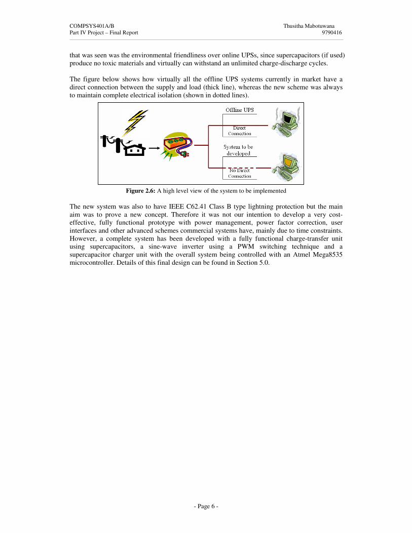
that was seen was the environmental friendliness over online UPSs, since supercapacitors (if used) produce no toxic materials and virtually can withstand an unlimited charge-discharge cycles. The figure below shows how virtually all the offline UPS systems currently in market have a direct connection between the supply and load (thick line), whereas the new scheme was always to maintain complete electrical isolation (shown in dotted lines).
Figure 2.6: A high level view of the system to be implemented The new system was also to have IEEE C62.41 Class B type lightning protection but the main aim was to prove a new concept. Therefore it was not our intention to develop a very cost-effective, fully functional prototype with power management, power factor correction, user interfaces and other advanced schemes commercial systems have, mainly due to time constraints. However, a complete system has been developed with a fully functional charge-transfer unit using supercapacitors, a sine-wave inverter using a PWM switching technique and a supercapacitor charger unit with the overall system being controlled with an Atmel Mega8535 microcontroller. Details of this final design can be found in Section 5.0.

COMPSYS401A/B Thusitha Mabotuwana Part IV Project – Final Report 9790416
- Page 7 -
3.0 Development of the Design The development process was broken down mainly into 4 stages. First was the research and analysis phase and second was identifying the individual modules involved in the complete system and deciding suitable implementation strategies. The third stage was the testing phase where selected options were experimented. The last stage involved deciding on the final options and developing the prototype. The first 2 were considered very important since most of the decisions pertaining to the final implementation were made during these stages. As such, the complete system was studied and many possibilities were considered out of which only a few were chosen to be tested. This elimination process was given a lot of thought and many meetings were held with the project supervisor to ensure that only the most time-consuming and difficult solutions that definitely could not be implemented within the given time were eliminated. This section outlines the different aspects of the overall system and various options considered, along with some of the preliminary decisions that were made.
3.1 Research and Analysis Phase The implemented final solution is the outcome of many successive preliminary stages out of which this can be considered the first. During this stage the complete system behaviour was studied and the system was broken down into smaller modules using a systems approach. Many journal papers, publications and other literature were read to see how others have implemented similar systems and what schemes were used. This gave us a good knowledge on the state-of-art techniques but it was also understood that the new approach involved many new concepts where much literature was not readily available. This also meant that we had to develop our own schemes and try out many experiments ourselves instead of following standard procedures. After much research and analysis, six different modules were identified as subsystems of the overall system and various possible implementation techniques were considered for each one, as detailed out in Section 3.1.1.
3.1.1 System Overview The six main modules that were identified are shown in Figure 3.1. An outline of each module follows.
Figure 3.1: Block diagram of the overall system

COMPSYS401A/B Thusitha Mabotuwana Part IV Project – Final Report 9790416
- Page 8 -
1. Energy Pump:
This block was to rectify the 230V, 50Hz input given by the mains supply. Whenever a supercapacitor bank needed to be charged, the controller subsystem was to set appropriate control signals and establish electrical connectivity between the bank and this module’s output.
2. Charge Transfer Unit This was to consist of multiple, self-contained charge holding devices. The main aim of this unit was to continuously supply energy to the inverter by means of some switching mechanism while providing common and differential mode isolation. To maintain uninterrupted power at the inverter end, it was required to always have a supercapacitor bank connected to the inverter’s inputs. Part of the discharging bank’s energy was also to be used to power-up the backup battery charger whenever this needed to be used. In case of a high voltage transient there is a possibility of the charging bank blowing up; hence a few redundant banks were also to be used.
3. Inverter
The input to the inverter was to be from the supercapacitor banks or from the battery. The former was to be used under normal operating conditions whereas the latter used only to provide the energy in the event of a blackout. The input to this inverter block was decided to be around 12VDC which is then converted to 230VAC, 50Hz at its output.
4. Battery Backup
This was to be used to power-up the controller subsystem since the controller needs to be protected from any incoming surges. Also it was to be used to supply power to the load for about fifteen minutes under any blackout conditions.
5. Charger for Battery Backup This module’s task was to recharge the battery whenever it reached a certain minimum voltage.
6. Controller Subsystem
The controller was to ensure correct and timely functionality of the overall system. It was to monitor the line voltages to detect any incoming surges, switch the capacitor banks to guarantee uninterrupted power at the inverter, regulate the output end and also monitor battery health.
3.1.2 Options Considered and Preliminary Design Decisions
This section does not intend to give a detailed analysis of all the options considered and analysed since all this information has already been presented in the interim reports. The aim is to give an overview of the options considered and a brief outline of the options that were decided to be experimented. Please refer to the interim reports [9,10] for a complete, detailed analysis of all the options. Options considered for the charge holding devices were supercapacitors (double layer capacitors and ultra capacitors), inductors and batteries. Supercapacitors were chosen over the others mainly due to the properties described in Section 2.3. For the energy pump, a current source was to be used to charge the supercapacitors at a constant rate. Three options, direct rectification of the mains supply, line frequency step down transformer with a rectifier, and using a switching device to increase the mains supply frequency and then using a high frequency step down transformer with a rectifier were considered out of which the

COMPSYS401A/B Thusitha Mabotuwana Part IV Project – Final Report 9790416
- Page 9 -
last option was selected as the best. Main reasons were ease of control, simplicity, cost and good electrical isolation [9]. FPGAs, DSPs and microcontrollers were considered for the controller subsystem and microcontroller was chosen as a suitable controller system. An Atmel Mega64 microcontroller was chosen among many others considered. The main reasons behind this were I/O pins required, clock frequency, ADC channels and availability of the chip and a suitable development system (CodeVision AVR) within the department. Please refer to Appendix B for details on this selection process. For the inverter module, switch mode topologies such as PWM, PAM, square wave modulation and voltage cancellation; and resonant topologies such as Class D, Class E, self sustained and energy injection; and high frequency links, which is a mixed topology were among the various schemes that were looked at. However only the switch mode topologies and the self sustained scheme were decided to be tested, mainly due to their ease of control and implementation [9]. A 1800mAh NiCd battery was decided to be used for the backup unit along with a commercially available charger, but these two modules were given less priority over the others since these are required mainly in a final product implementation and not in a proof-of-concept design. Also the time restrictions of the project made spending time on these modules almost infeasible. Therefore these 2 modules are shown in dotted lines in Figure 3.1.
3.2 Implementation of the Selected Options During this stage of the development process, the options that were short-listed in the research and analysis phase were bred-boarded and tested. An STK200 development board and an Atmel 90S8535 microcontroller 2 were borrowed from Mr. Grant Sargent and the required supercapacitors were borrowed from our project supervisor Mr. Nihal Kularatna. This saved us a lot of project funding which would simply have been inadequate due to the high cost of these components. Also a commercially available inverter was purchased with the project funding since I could work on the control aspects of the complete system using this while Mr. Thrimawithana was working on the inverter design. Details and key results obtained during the preliminary stages are described in Section 4.0.
2 This microcontroller was readily available and had sufficient resources to support the system at this early stage. This was used since the chosen Mega64 microcontroller was not available in the Department store.

COMPSYS401A/B Thusitha Mabotuwana Part IV Project – Final Report 9790416
- Page 10 -
4.0 Design Process and Preliminary Results This section details out some important results obtained during the preliminary stages of the development process. Details of control algorithms and experimental results pertaining to the microcontroller and the charge transfer unit are given in Section 4.1. Section 4.2 discusses the inverter module and various experiments carried out.
4.1 Microcontroller – Charge Transfer Unit Interface
The charge transfer unit consist of multiple, self-contained supercapacitor bank modules and the purpose was to continuously supply the load by means of some switching scheme, while providing common and differential mode isolation. Two main techniques were considered to achieve the above functionality: 1. Using the microcontroller’s Analogue-to-Digital Converter (ADC) channels to monitor the
bank voltage levels and decide fully-charged and fully-discharged conditions. 2. Using analogue circuitry to determine fully-charged and fully-discharged conditions and
sending logic high or low signals to the controller to indicate any status changes. Discussed in the following sections are details of the above two techniques.
4.1.1 Analogue Interface with ADC Inputs
4.1.1.1 Simulation of charge-transfer unit using power supplies
During the initial stages of this phase, before Mr. Thrimawithana finished developing the architecture for the supercapacitor bank module, the bank voltages were simulated using 3 power supply voltages (Figure 4.1). The idea behind this was to develop the required switching algorithms in parallel with the hardware implementation and then simply replace the power supplies with the actual supercapacitor bank modules, once designed.
`
Figure 4.1: An initial setup used to simulate bank voltages The requirement was to cycle these power supplies in software in such a way that at any given time the supply connected to the load was not connected to the input. After the supply connected to the load reached a pre-defined minimum voltage it had to be charged again to a pre-defined maximum level. However before moving this supply to charging, a different supply that already had finished charging had to be connected to the load to maintain uninterrupted supply to the load. The above mentioned pre-defined minimum and maximum voltages simply allow the user to
Power Supply 0
Power Supply 1
Power Supply 2
Microcontroller (90S8535)
ADC inputs Display
bank status on terminal
PC

COMPSYS401A/B Thusitha Mabotuwana Part IV Project – Final Report 9790416
- Page 11 -
change the output Vrms and the output voltage ripple and these values were globally defined in the program and could easily be changed by simply entering the new values in. At this stage of the design the actual charging-discharging times of the supercapacitors were not known with precision, but were roughly calculated as follows to determine the ADC sampling frequency: From equations itQ = and CVQ = , t was estimated to be around 50ms assuming we’d be using supercapacitors of 1F with a voltage ripple of around 0.5V at its output and that a charging current of 10A will be used. Also if 10 sampling points were to be taken from each bank, the required sampling interval would be 5ms. The microcontroller’s main clock frequency was 4MHz and various possible sampling rates were calculated as shown in Table 4.1.
Division Factor
ADC Clock (kHz)
ADC Clock Period (µs)
Sampling Interval = 13 ADC Cycles (µs)
2 2000 0.5 6.5 4 1000 1 13 8 500 2 26
16 250 4 52 32 125 8 104 64 62.5 16 208 128 31.25 32 416 Table 4.1: Various possible sampling rates with a 4MHz main clock [11]
Since three banks had to be monitored and the ADC channels were polled, in order to maintain a 5ms sampling interval per channel, each ADC channel had to be monitored at least 3 times as fast, or at a 1.33ms sampling interval. Therefore using a division factor of 128, an ADC clock of 31.25kHz was obtained with 10-bit resolution. This provided an accuracy of approximately 5mV as shown in the calculation below. Maximum ADC input voltage = 5V Number of ADC values using 10-bits = 1023 ∴Accuracy = 5/1023V = 0.004888V ≈ 0.005V The microcontroller was programmed to poll3 the analogue inputs and the charging-discharging cycle of the supercapacitor banks was simulated by manually changing the supply voltages and carefully observing the displayed status change. For example let’s assume that all the supplies had a voltage level of 4V and that supply 1 was discharging. Now if supply 1’s voltage was to drop to say 2V which was pre-defined to be the fully discharged threshold, a different supply (say supply 0 or 2 in this case) was to take supply 1’s position and supply 1 was to charge and reach the pre-defined maximum threshold, or fully-charged voltage (say 4V). To meet this requirement, a finite state machine (FSM) with 4 states was developed where each supply (let’s call each power supply a bank or a supercapacitor bank from now on since this is what each supply represents) could be in CHARGING, STANDBY, DISCHARGING or CHARGING QUEUE state. Figure 4.2 shows these four different states and how they were to change depending on the current voltage levels.
3 Here polling means the scanning process of ADC inputs, one-by-one

COMPSYS401A/B Thusitha Mabotuwana Part IV Project – Final Report 9790416
- Page 12 -
Figure 4.2: State diagram showing supercapacitor bank states In order to implement the above FSM, the 3 supercapacitor banks were named bank0, bank1 and bank2 and a structure was created in software for each bank to hold the bank’s voltage and current state. When the system first starts up, the microcontroller would wait for all the banks to reach the minimum required voltage (or fully-charged condition which also implies that all banks have been initialised) before progressing any further. It was assumed that all the banks were functional and would reach the minimum charged voltage within finite time. Also it was decided to have only 1 bank in CHAGING state so that the energy pump would always have to provide a constant current to charge the banks. Shown Figure 4.3 is a flowchart of the control process that was used to implement the above FSM.
Supercapacitor hasn’t reached full-charged
voltage
No supercapacitor in Charging mode
Discharging bank needs to be changed
Supercapacitor fully-charged, but other capacitor in discharging mode
Supercapacitor fully charged
Discharging bank reached a minimum
voltage
Discharging
bank
Charging Queue banks
Charging
bank
Stand-by
banks
Supercapacitor needs charging, but other supercapacitor in Charging mode

COMPSYS401A/B Thusitha Mabotuwana Part IV Project – Final Report 9790416
- Page 13 -
Figure 4.3: Flowchart showing a basic switching mechanism After initialisation, bank0’s status was arbitrarily set to DISCHARGING and the other 2 banks modes set to STANDBY. When bank0’s voltage reached a pre-specified minimum (MIN), bank1’s status is set to DISCHARGING and bank0’s status is set to CHARGING QUEUE. In the next ADC cycle, bank0s status will be set to CHARGING as there is no other bank in CHARGING mode. After bank0 reaches the maximum voltage (MAX) its status will then be set to STANDBY. After cycling through the same mechanism for banks 1 and 2, the process is once again repeated for all banks starting from bank0. A flag bit was also used in the above algorithm to ensure that 2 banks were never in CHARGING state at the same time.
4.1.1.2 Charge-transfer unit with hardware The above process was perfected for all possible input variations and the next step was to replace the DC power supplies with the actual supercapacitor banks. The supercapacitors we were using were 0.2F (although initially it was assumed 1F supercapacitors would be available to us) with the output ripple set to 1V in software. The charging current used was 6A which gives a charging time of approximately 33ms. As 3 banks were to be used and the banks were polled, each bank’s voltage had to be checked at least every 11ms. Assuming 10 sampling points were to be taken,
CHARGING QUEUE Yes
No
< MIN
� MAX
Yes
Reset
Main loop (Stay infinitely)
ADC INT occurred?
Read ADC value
All caps initialised?
Cap voltage
Bank in CHARGING
mode
Set switching signals and next
ADC channel
Status
Set bank status to STANDBY
If no bank is currently in CHARGING mode, change status to CHARGING
Find a bank in STANDBY and set its status to DISCHARGING. Set current bank’s status to CHARGING QUEUE
Yes
No
DISCHARGING
System Initialisation
No

COMPSYS401A/B Thusitha Mabotuwana Part IV Project – Final Report 9790416
- Page 14 -
R2Vc-
Vout
Capacitor Bank
Vc+
Vc
ADC Port
OPAMP
+
-
OUT
R1
R2
Micro Ground
R1
Microcontroller
ADC Pin 0M1
V_Driv e (20V)
Pins 0-8
PVI
C1
R1
C2
Pins 0-8PortB Pin 0
M2
C3
D1
ADC
Driv er
PortC Pin 0
PortB
Pins 0-8
PortC
MicroOutput(Controlled)
Input > 14V
the sampling interval would be 1.1ms, hence the same 31.25kHz ADC clock was used as before to monitor the banks. Also required code was added to turn the FET switches on and off during the transitions. During the integration process one key concept had to be paid attention to, and that was maintaining the common and differential mode isolation. In Figure 4.1 when the banks were simulated using DC sources, the ground planes were made common which could not be so with the self-contained modules. Therefore level shifting circuitry was required to refer the supercapacitor bank’s voltage to the microcontroller’s ground plane. Shown below in Figure 4.4 is such a level shifting circuit.
Figure 4.4: A level shifting circuit that refers a bank’s output to the microcontroller’s ground plane [12]
Vout can be changed by suitably choosing values for R1 and R2. For our requirements R1 and R2 were chosen to give a maximum of 5V at the maximum capacitor rated voltage since this (5V) is the maximum limit that can be given to an ADC channel. The architecture of a supercapacitor bank module used during this stage is shown in Figure 4.5.
Figure 4.5: Circuit diagram of a supercapacitor bank during an early stage [8]

COMPSYS401A/B Thusitha Mabotuwana Part IV Project – Final Report 9790416
- Page 15 -
In the circuit in Figure 4.5, switches M1 and M2 were controlled by the microcontroller and switch M1 was driven with a logic high (or 5V) when the bank’s status was CHARGING. Switch M2 was turned ON when the bank’s status was DISCHARGING. It was also ensured that both switches, M1 and M2 were never turned ON simultaneously in order to always provide complete input-output isolation. However when the algorithm in Figure 4.3 was integrated with the actual components, the banks did not switch as expected. The 2 main conditions that were checked in the controller were greater than maximum and less than minimum conditions. Debugging of the system proved that the supercapacitor banks had a transient such that there was a slight increase in bank voltage as soon as it was disconnected from the load (Figure 4.6).
Figur 4.6: Supercapacitor voltage rise when disconnected from load The bank was in CHARGING QUEUE mode and its voltage was expected to be less than the fully-discharged voltage. However due to the unexpected and unknown increase in voltage, it was in CHARGING QUEUE state, but with a slightly greater than fully-discharged voltage. This made the bank rest in an intermediate state and became undetected by any of the conditions within the 2 main conditions. In order to account for this unexpected supercapacitor characteristic, the switching algorithm was modified as shown in Figure 4.7. Instead of checking only for the voltage levels and then determining the state, voltage level and state both were checked simultaneously and then the next state was determined.
Bank Voltage
Time
Unexpected voltage increase of supercapacitor bank after being disconnected from load

COMPSYS401A/B Thusitha Mabotuwana Part IV Project – Final Report 9790416
- Page 16 -
Figure 4.7: Flowchart showing an enhanced switching mechanism Using an ADC clock of 31.25kHz gives a sampling interval of approximately 416µs x 3, or 1.248ms for each bank. However experiments showed that the supercapacitor bank charging time was only around 5-6ms as opposed to the 33ms calculated before due to current and output voltage ripple variations (Figure 4.8).
Figure 4.8: Waveform showing current drawn by a supercapacitor bank during charging A 5ms charging time could not be monitored with sufficient time domain resolution using the current speed of the ADC clock. The result of this was the supercapacitors charging over the
Cap not found
Cap
found
Yes
No
goto main loop of Figure 4.3
Similar to Figure 4.3
All caps initialised?
Cap voltage and
status
CHARGING and V � MAX
CHARGING QUEUE and flag: bankCharging = 0
DISCHARGING and V < MIN
Set bank status to STANDBY. Set flag: bankCharging = 0
Find bank with lowest voltage from the queue and set status to CHARGING. Set flag: bankCharging = 1
Set current bank’s status to CHARGING QUEUE and standby
cap’s status to DISCHARGING
Find a STANDBY cap
with lowest voltage
Set switching signals if required and next
ADC channel
Otherwise
Set next ADC channel

COMPSYS401A/B Thusitha Mabotuwana Part IV Project – Final Report 9790416
- Page 17 -
desired maximum limit. Although higher sampling rates were tried out using lower division factors of the main clock, this reduced the resolution of the samples down to 7-8 bits compared to 10. Also after accounting for the lines of code the microcontroller had to possibly execute in the final implementation it was decided to change the main clock to a 16MHz oscillator. Although it was decided to change the processor, a resistor was placed in series with the charger to increase the bank charging time merely to check if the concept could be implemented. The following waveform was obtained for a resistive load of a few ohms and complied with the expected waveform. This was a key result obtained that proved to us that the concept of transferring energy by switching supercapacitor banks appropriately was realisable and could be implemented.
Figure 4.9: Waveform showing how a supercapacitor bank is switched In the above waveform it appears that only banks 1 and 2 are being switched. This is because the algorithm was coded in such a way that the status of the bank with the lowest voltage was first updated. For example if banks 0 and 1 are in STANDBY mode with voltages of 13.2V and 13.1V respectively, bank1’s status will be set to DISCHARGING when required since it has the lowest voltages out of all the banks in STANDBY mode. Due to the non-identical characteristics (self-discharging rate etc.) of the supercapacitor banks, banks 1 and 2 always had a slightly higher voltage than bank0, hence the above waveform. However this algorithm was modified in the final implementation to equally use all the banks so that all the supercapacitors undergo the same number of charge-discharge cycles. The next important step in the controller design was to monitor the bank charging times so that the 5ms charging time could be detected. This definitely could not be achieved using the STK200 board with a 4MHz oscillator, therefore an STK500 development board was borrowed from Mr. Aaron Taylor with a 16MHz oscillator. An Atmel Mega8535 microcontroller which has exactly the same features as the previous one, but supports the higher clock frequency was used with this new development system. Now the ADC conversion time with the same division factor of 128 and resolution was reduced to 104µs compared to the 416µs of the previous, enabling us to detect the bank voltages properly. The new ADC conversion times are shown in Table 4.2.
Charging logic
Discharging logic
Supercapacitor Output waveform {
{{
COMPSYS401A/B Thusitha Mabotuwana Part IV Project – Final Report 9790416
- Page 18 -
Division Factor
ADC Clock (MHz)
ADC Clock Period (µs)
Sampling Interval = 13 ADC Cycles (µs)
2 8 0.125 1.625 4 4 0.25 3.25 8 2 0.5 6.5 16 1 1 13 32 0.5 2 26 64 0.25 4 52 128 0.125 8 104
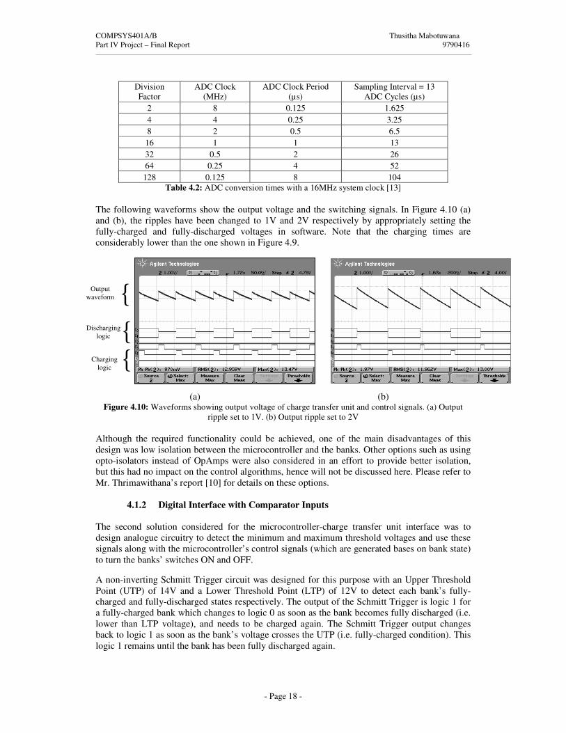
Table 4.2: ADC conversion times with a 16MHz system clock [13] The following waveforms show the output voltage and the switching signals. In Figure 4.10 (a) and (b), the ripples have been changed to 1V and 2V respectively by appropriately setting the fully-charged and fully-discharged voltages in software. Note that the charging times are considerably lower than the one shown in Figure 4.9. (a) (b)
Figure 4.10: Waveforms showing output voltage of charge transfer unit and control signals. (a) Output ripple set to 1V. (b) Output ripple set to 2V
Although the required functionality could be achieved, one of the main disadvantages of this design was low isolation between the microcontroller and the banks. Other options such as using opto-isolators instead of OpAmps were also considered in an effort to provide better isolation, but this had no impact on the control algorithms, hence will not be discussed here. Please refer to Mr. Thrimawithana’s report [10] for details on these options.
4.1.2 Digital Interface with Comparator Inputs
The second solution considered for the microcontroller-charge transfer unit interface was to design analogue circuitry to detect the minimum and maximum threshold voltages and use these signals along with the microcontroller’s control signals (which are generated bases on bank state) to turn the banks’ switches ON and OFF. A non-inverting Schmitt Trigger circuit was designed for this purpose with an Upper Threshold Point (UTP) of 14V and a Lower Threshold Point (LTP) of 12V to detect each bank’s fully-charged and fully-discharged states respectively. The output of the Schmitt Trigger is logic 1 for a fully-charged bank which changes to logic 0 as soon as the bank becomes fully discharged (i.e. lower than LTP voltage), and needs to be charged again. The Schmitt Trigger output changes back to logic 1 as soon as the bank’s voltage crosses the UTP (i.e. fully-charged condition). This logic 1 remains until the bank has been fully discharged again.
Discharging logic
Output waveform
Charging logic
{{{
COMPSYS401A/B Thusitha Mabotuwana Part IV Project – Final Report 9790416
- Page 19 -
The logic signals generated by the Schmitt Trigger were fed into the microcontroller which were then used in conjunction with the microcontroller’s control signals to generate the following truth table.
Table 4.3: Table showing charging logic based on control logic and Schmitt Trigger output The above logic cannot be simplified into any simple standard logic. However if the microcontroller’s control signals were chosen as active-low, the truth table shown in Table 4.4 can be obtained which can be simplified into standard NOR logic.
Table 4.4: Table showing charging logic based on inverted control logic and Schmitt Trigger output
The main advantage of this design was that the charging switch was automatically turned off (irrespective of microcontroller logic) as soon as the bank’s voltage reached the fully-charged voltage. Although the standard NOR chip’s specified gate delay was approximately 8ns [14], this could safely be ignored since the change in a bank’s voltage within this time duration was almost negligible. Another advantage was that this method provided better isolation compared to using ADC inputs since the output of the Schmitt Trigger could be sent through opto-isolators without having to account for any steady state error due to opto-isolator dissimilarities. The logic shown in Table 4.4 was used in the implementation in a similar way to the ADC scheme, but instead of checking for the voltage conditions, logic high or low conditions of the Schmitt Trigger were tested when deciding a bank’s state. Also all the testing was done in the main loop since there was no need for an interrupt service routine as with the ADC scheme. However this scheme had a few major drawbacks. First was that the microcontroller was not getting the actual bank voltage. Although this voltage was not required for any of the control algorithms and could be implemented using a purely digital mechanism as above, this gave less control to the controller over the circuitry, especially when required to check for possibly destroyed or non-functional banks. The other main drawback of this method was that the hardware had to be changed every time the charging-discharging limits (UTP and LTP) were changed, whereas with the previous method these limits could be set in software. Therefore this mechanism to control the banks was not preferred over the previous.
4.2 Control Provided for Inverter Topologies
For the inverter it was decided to implement a single stage, push-pull type scheme4. The main topologies considered for the inverter were resonant, PWM and PAM which are briefly discussed in the following sections.
4 Please refer to Mr. Thrimawithana’s report for details on this decision.
Microcontroller logic (1-ON, 0-OFF) Schmitt Trigger Output Bank Charging Signal
(1-ON, 0-OFF) 0 0 0 0 1 0 1 0 1 1 1 0
Microcontroller logic (1-OFF, 0-ON) Schmitt Trigger Output Bank Charging Signal
(1-ON, 0-OFF) 0 0 1 0 1 0 1 0 0 1 1 0

COMPSYS401A/B Thusitha Mabotuwana Part IV Project – Final Report 9790416
- Page 20 -
D1Driv er
1 2
Driv erDriv er
12
Q2
D51 2
1 2
Q3
Q1
C1
Microcontroller
T1
Vin
D3
Self-resonant
circuit
Signal Generator 50Hz sine wave
AIN0
AIN1
4.2.1 Resonant Inverter
The first inverter topology that was tested was the resonant converter method. With this method a switch (Q1) was used to control the energy into the resonant tank. The switch was controlled by comparing the tank output with a 50Hz sine wave generated from the signal generator.
Figure 4.11: Self resonant inverter topology [modified from 12]
The analogue comparator of the microcontroller was used to compare the 2 waveforms. The comparator’s output is set (logic 1) if AIN0 is higher than AIN1 and logic 0 otherwise. The comparator interrupt was set to trigger on both the rising and falling edge of the comparator output. If triggered on a rising edge (i.e. AIN0 > AIN1) the control signal to the driver block in Figure 4.12 was set to 0 to turn Q1 OFF. This control signal was set to logic 1 to turn Q1 ON when the tank’s output was less than the amplitude of the sine wave. Figure 4.12(a) shows the output obtained with the above setup. As can be seen in the figure, the output fails to follow the input as expected due to the energy stored in the resonant tank. However this setup worked fine when the system was run at 10Hz (instead of 50Hz) as shown in Figure 4.12(b).
(a) (b) Figure 4.12: Output of resonant tank with a frequency of (a) 50Hz. (b) 10Hz

COMPSYS401A/B Thusitha Mabotuwana Part IV Project – Final Report 9790416
- Page 21 -
4.2.2 Push-pull Square / PWM Inverter
As a first stage of a PWM inverter design, a square wave push-pull inverter scheme was tested (in an open-loop configuration) and the control signals were generated using a simple 0.1ms timer interrupt. Within the timer Interrupt Service Routine (ISR), 2 of the microcontroller’s pins were written logic 1 or 0 depending on whether the switch had to be turned ON or OFF respectively. Switch Q1 in Figure 4.13(a) is used to generate the positive half of the output while Q2 is used to produce the negative half of the sine wave. Therefore it had to be ensured that both the switches Q1 and Q2 were never turned ON at the same time. Within the ISR the pin that was logic 1 (or ON) was first written a logic 0 and then the other switch turned ON to achieve this. Also a small delay was introduced between turning a switch OFF and turning the other one ON to reduce the harmonics in the output. The 0.1ms timer overflow interrupt was generated using the 8-bit timer0 of the chip and the reload value was calculated as follows: Using a division factor of 64 of the 16MHz main clock gives a sub-clock of 250kHz which has a period of 4µs. Since we need a 0.1ms interrupt, this needs 250 ticks of the sub-clock. timer0 is an 8-bit timer which overflows every 256 of its clock ticks, therefore should be reloaded with the number 6 (which is 256-250). A satisfactory waveform shown in Figure 4.13(b) was obtained at the output. Figure 4.13(a) shows the inverter circuit used.
(a)
(b) Figure 4.13: (a) Circuit [12] (b) Output waveform of a push-pull square wave inverter
Rl
Vc
1 2
Driv er
T1
Capacitor Bank
Microcontroller
D1
12
Q3
D3
1 2
Q2
Driv er
Q1 Q2

COMPSYS401A/B Thusitha Mabotuwana Part IV Project – Final Report 9790416
- Page 22 -
The transformer that was being used in the inverter was a 50Hz, 230-12V step-down transformer used in a step-up configuration. Although theoretically we should have been able to get 230Vrms at the actual transformer’s primary by giving 12V to the secondary, the transformer’s maximum output was only around 190Vrms as can be seen in Figure 4.14(b). With the supervisor’s consent, the project specifications were changed at this point to implement a 110Vrms scheme instead of a 230Vrms since we did not have the option of getting a proper 50Hz step-up transformer. Also our aim was to generate a sinusoidal output at the inverter end; hence a sine modulated PWM scheme had to be implemented instead of a square wave scheme. The idea was to drive the inverter switches with a suitable PWM control signal and then use only the fundamental frequency at the output by filtering out the other high frequency components (Figure 4.14).
Figure 4.14: Scheme to be implemented with the PWM switching scheme [15] However generating this required PWM was not a very simple task since the output of the inverter (feedback loop) had to be first compared with the required 50Hz waveform and then compare this error signal with a selected 1kHz saw-tooth waveform as shown below.
Figure 4.15: Graph showing how PWM signal is generated for PWM inverter Two main possibilities were considered to generate this PWM, which had to be high if the error signal was greater than the saw tooth and low otherwise.
1. Generate the 50Hz sine and the 1kHz saw tooth waveforms from the microcontroller and then use analogue design to compare the inverter output with the 50Hz one and then compare this error signal with the saw tooth waveform using the microcontroller’s analogue comparator.
2. Use the microcontroller to internally do all the processing (sine wave comparisons etc.) and simply output the required PWM.
Both these options have the advantage of removing some of the undesired harmonics, however the first option was decided to be tested due to ease of control. The following steps were carried out to generate the precise sampling points to fit in exactly 20 periods of the saw tooth waveform into 1 period of the 50Hz sine wave:
1kHz saw tooth waveform
50Hz error signal
Inverter control PWM

COMPSYS401A/B Thusitha Mabotuwana Part IV Project – Final Report 9790416
- Page 23 -
1. In order to have sufficient resolution, it was arbitrarily decided to have 10 sampling points within each saw tooth waveform period giving a sampling time of 0.1ms (Figure 4.16).
Figure 4.16: Digital saw tooth waveform that was to be generated
2. After considering possible sampling points for the sine wave, points 0,4,8,2,6 (marked with
‘x’s) of the above waveform were considered suitable since they follow a certain pattern and repeat every 2 periods of the saw tooth.
3. The DAC values were calculated using the formula: DAC value = required voltage (from Figure 4.17) x 255 / 5;
4. The above values were entered into 2 lookup tables, one for the saw tooth and one for the sine.
5. An external DAC was used with the Serial Peripheral Interface (SPI) of the microcontroller to output the 2 required waveforms with the setup shown in Figure 4.17
Figure 4.17: Block diagram showing setup for PWM inverter
Inverter output
Inverter (PWM)
Error amplifier
Microcontroller
Analogue Comparator
Commands and DAC data
SPI interface
50Hz sine wave
Error signal
1kHz saw tooth wave
Inverter control
External DAC (Analog Devices – DAC8800)
x
x
x
x
x

COMPSYS401A/B Thusitha Mabotuwana Part IV Project – Final Report 9790416
- Page 24 -
Shown below in Figure 4.18(a) is the output of the DAC without any filtering. Figure 4.18(b) shows the same waveforms with a capacitor used as a filter across the 2 outputs.
Figure 4.18: 50Hz sine and 1kHz saw tooth waveforms: (a) without filtering (b) with capacitors used to filter out the 2 signals.
Although this scheme has the advantage of phase cancellation, it proved to be rather difficult to implement. The 50Hz, 12V-230VAC commercial transformer that was being used was making considerable noise, and controlling the inverter in a feedback loop proved to be tedious. Figure 4.19 shows the output of the inverter without the feedback loop being implemented (i.e. instead of comparing the saw tooth with the error signal, it was compared directly with the 50Hz sine wave generated from the microcontroller). The second technique was not tried out mainly due to the large overhead required for which a DSP system would be more suitable.
Figure 4.19: Output of the PWM inverter An RMS control strategy was developed for the final implementation which uses the microcontroller to monitor the output voltage and adjust the driving PWM accordingly. This technique is discussed in Section 6.0.
COMPSYS401A/B Thusitha Mabotuwana Part IV Project – Final Report 9790416
- Page 25 -
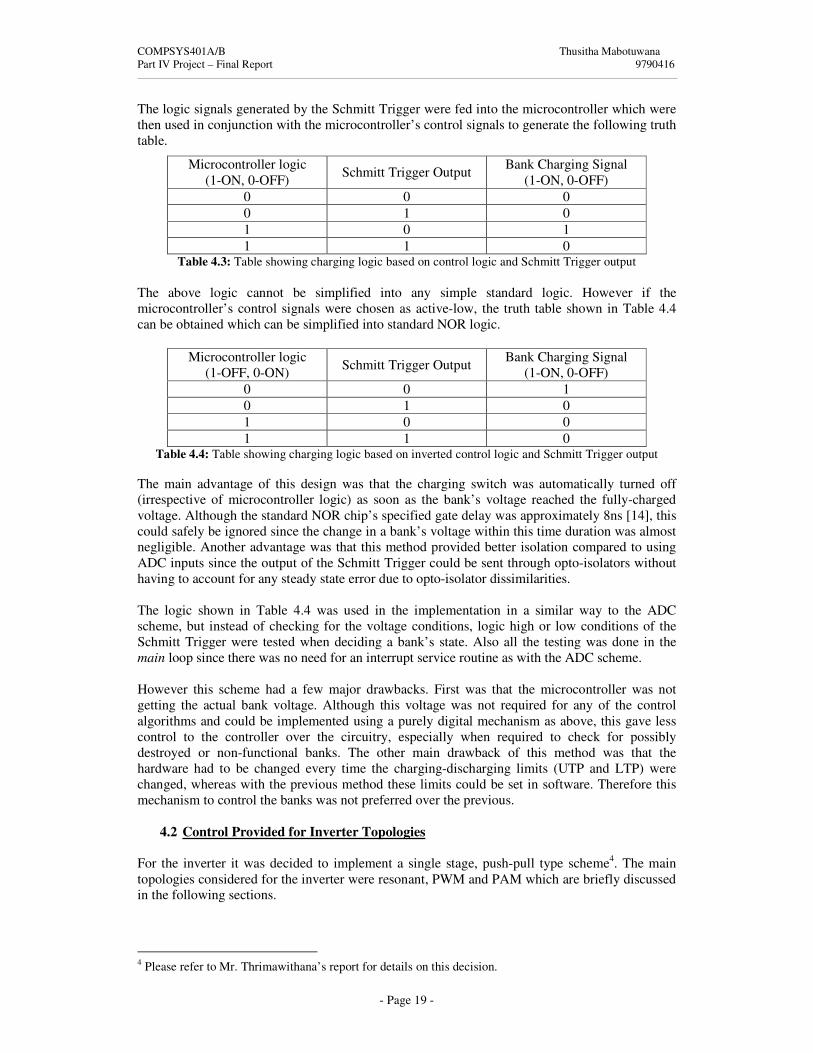
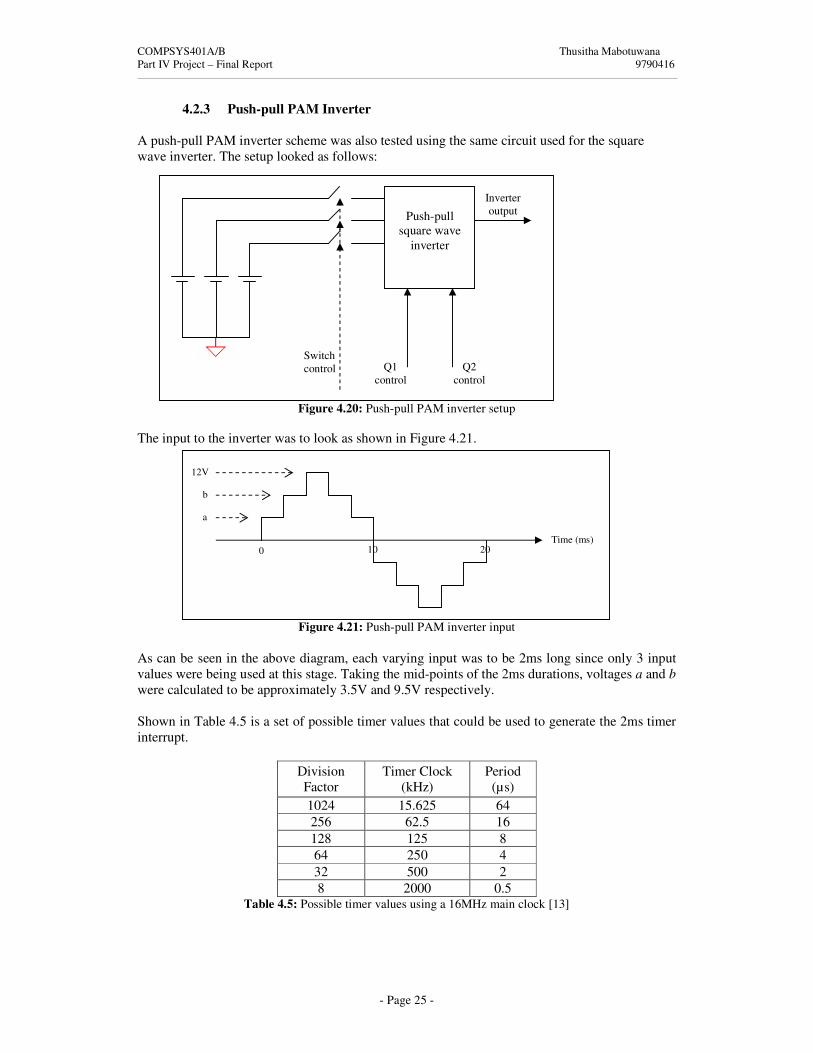
4.2.3 Push-pull PAM Inverter A push-pull PAM inverter scheme was also tested using the same circuit used for the square wave inverter. The setup looked as follows:
Figure 4.20: Push-pull PAM inverter setup
The input to the inverter was to look as shown in Figure 4.21.
Figure 4.21: Push-pull PAM inverter input As can be seen in the above diagram, each varying input was to be 2ms long since only 3 input values were being used at this stage. Taking the mid-points of the 2ms durations, voltages a and b were calculated to be approximately 3.5V and 9.5V respectively. Shown in Table 4.5 is a set of possible timer values that could be used to generate the 2ms timer interrupt.
Division Factor
Timer Clock (kHz)
Period (µs)
1024 15.625 64 256 62.5 16 128 125 8 64 250 4 32 500 2 8 2000 0.5
Table 4.5: Possible timer values using a 16MHz main clock [13]
Q1 control
Push-pull
square wave inverter
Q2 control
Inverter output
Switch control
0 Time (ms)
10 20
a
b
12V
COMPSYS401A/B Thusitha Mabotuwana Part IV Project – Final Report 9790416
- Page 26 -
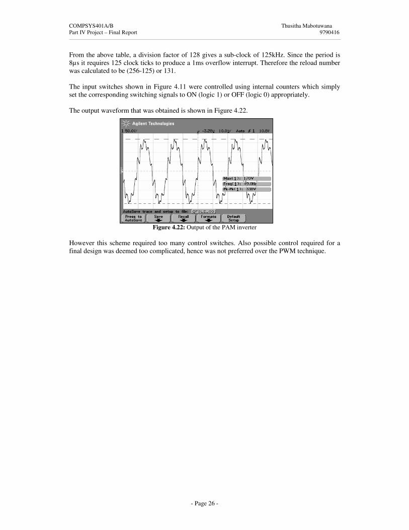
From the above table, a division factor of 128 gives a sub-clock of 125kHz. Since the period is 8µs it requires 125 clock ticks to produce a 1ms overflow interrupt. Therefore the reload number was calculated to be (256-125) or 131. The input switches shown in Figure 4.11 were controlled using internal counters which simply set the corresponding switching signals to ON (logic 1) or OFF (logic 0) appropriately. The output waveform that was obtained is shown in Figure 4.22.
Figure 4.22: Output of the PAM inverter However this scheme required too many control switches. Also possible control required for a final design was deemed too complicated, hence was not preferred over the PWM technique.
COMPSYS401A/B Thusitha Mabotuwana Part IV Project – Final Report 9790416
- Page 27 -
5.0 Implementation of the Final Design
The previous section presented some preliminary experiments that were carried out and results obtained. This section details out the algorithms, control and implementation strategies developed for the final prototype. Section 5.1 discusses the energy pump design and control and Section 5.2 focuses on the energy transfer unit. Details pertaining to the inverter are in Section 5.3. Finally in Section 5.4 system integration issues are discussed.
5.1 Energy Pump
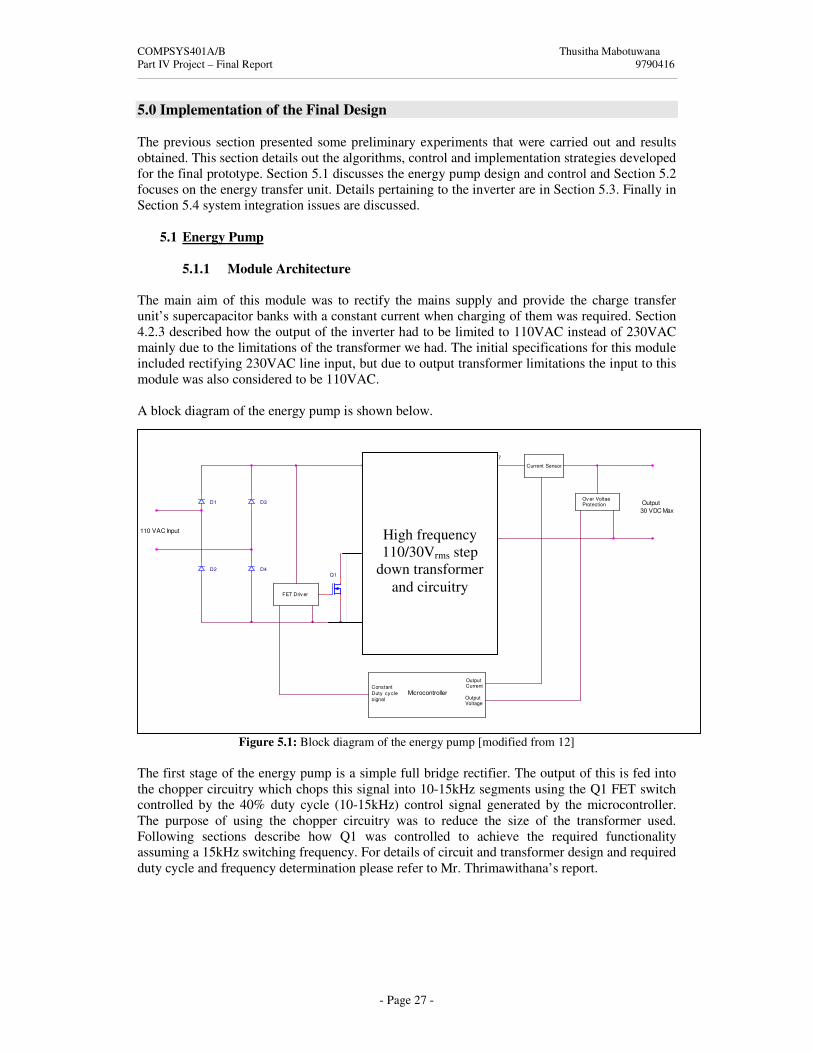
5.1.1 Module Architecture The main aim of this module was to rectify the mains supply and provide the charge transfer unit’s supercapacitor banks with a constant current when charging of them was required. Section 4.2.3 described how the output of the inverter had to be limited to 110VAC instead of 230VAC mainly due to the limitations of the transformer we had. The initial specifications for this module included rectifying 230VAC line input, but due to output transformer limitations the input to this module was also considered to be 110VAC. A block diagram of the energy pump is shown below.
Figure 5.1: Block diagram of the energy pump [modified from 12] The first stage of the energy pump is a simple full bridge rectifier. The output of this is fed into the chopper circuitry which chops this signal into 10-15kHz segments using the Q1 FET switch controlled by the 40% duty cycle (10-15kHz) control signal generated by the microcontroller. The purpose of using the chopper circuitry was to reduce the size of the transformer used. Following sections describe how Q1 was controlled to achieve the required functionality assuming a 15kHz switching frequency. For details of circuit and transformer design and required duty cycle and frequency determination please refer to Mr. Thrimawithana’s report.
D7
1
2
Microcontroller
D3
D6
1
2
Ov er VoltaeProtection
Current Sensor
C1
OutputCurrent
D5
FET Driv er
D2
D1
ConstantDuty cyclesignal Output
Voltage
R1
RCDSnubber
1
2
Output30 VDC Max
D4
110 VAC Input
Q1
High frequency 110/30Vrms step
down transformer and circuitry
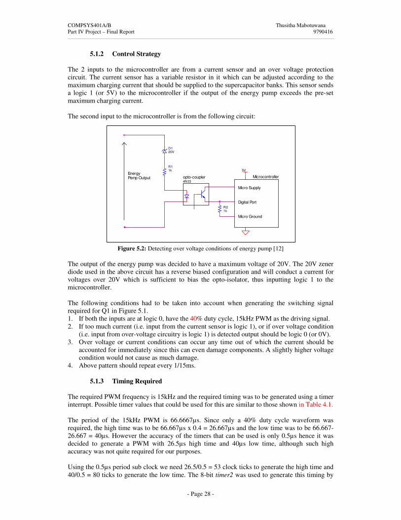
COMPSYS401A/B Thusitha Mabotuwana Part IV Project – Final Report 9790416
- Page 28 -
5.1.2 Control Strategy The 2 inputs to the microcontroller are from a current sensor and an over voltage protection circuit. The current sensor has a variable resistor in it which can be adjusted according to the maximum charging current that should be supplied to the supercapacitor banks. This sensor sends a logic 1 (or 5V) to the microcontroller if the output of the energy pump exceeds the pre-set maximum charging current. The second input to the microcontroller is from the following circuit:
Figure 5.2: Detecting over voltage conditions of energy pump [12] The output of the energy pump was decided to have a maximum voltage of 20V. The 20V zener diode used in the above circuit has a reverse biased configuration and will conduct a current for voltages over 20V which is sufficient to bias the opto-isolator, thus inputting logic 1 to the microcontroller. The following conditions had to be taken into account when generating the switching signal required for Q1 in Figure 5.1. 1. If both the inputs are at logic 0, have the 40% duty cycle, 15kHz PWM as the driving signal. 2. If too much current (i.e. input from the current sensor is logic 1), or if over voltage condition
(i.e. input from over-voltage circuitry is logic 1) is detected output should be logic 0 (or 0V). 3. Over voltage or current conditions can occur any time out of which the current should be
accounted for immediately since this can even damage components. A slightly higher voltage condition would not cause as much damage.
4. Above pattern should repeat every 1/15ms.
5.1.3 Timing Required The required PWM frequency is 15kHz and the required timing was to be generated using a timer interrupt. Possible timer values that could be used for this are similar to those shown in Table 4.1. The period of the 15kHz PWM is 66.6667µs. Since only a 40% duty cycle waveform was required, the high time was to be 66.667µs x 0.4 = 26.667µs and the low time was to be 66.667-26.667 = 40µs. However the accuracy of the timers that can be used is only 0.5µs hence it was decided to generate a PWM with 26.5µs high time and 40µs low time, although such high accuracy was not quite required for our purposes. Using the 0.5µs period sub clock we need 26.5/0.5 = 53 clock ticks to generate the high time and 40/0.5 = 80 ticks to generate the low time. The 8-bit timer2 was used to generate this timing by
EnergyPemp Output
R21k
R11k
opto-coupler
D1
Micro Supply
Micro Ground
Microcontroller4N33
5V
Digital Port
20V
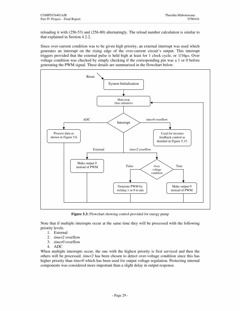
COMPSYS401A/B Thusitha Mabotuwana Part IV Project – Final Report 9790416
- Page 29 -
reloading it with (256-53) and (256-80) alternatingly. The reload number calculation is similar to that explained in Section 4.2.2. Since over-current condition was to be given high priority, an external interrupt was used which generates an interrupt on the rising edge of the over-current circuit’s output. This interrupt triggers provided that the external pulse is held high at least for 1 clock cycle, or 1/16µs. Over voltage condition was checked by simply checking if the corresponding pin was a 1 or 0 before generating the PWM signal. These details are summarised in the flowchart below.
Figure 5.3: Flowchart showing control provided for energy pump Note that if multiple interrupts occur at the same time they will be processed with the following priority levels.
1. External 2. timer2 overflow 3. timer0 overflow 4. ADC
When multiple interrupts occur, the one with the highest priority is first serviced and then the others will be processed. timer2 has been chosen to detect over-voltage condition since this has higher priority than timer0 which has been used for output voltage regulation. Protecting internal components was considered more important than a slight delay in output response.
Reset
Main loop (Stay infinitely)
Interrupt
Process data as shown in Figure 5.6
ADC
System Initialisation
timer0 overflow
Used for inverter feedback control as
detailed in Figure 5.15.
External timer2 overflow
Make output 0 instead of PWM Over
voltage condition
Generate PWM by writing 1 or 0 to pin
False True
Make output 0 instead of PWM

COMPSYS401A/B Thusitha Mabotuwana Part IV Project – Final Report 9790416
- Page 30 -
Micro Ground
Z
R2
Vz
Vc
5V
Vf
R1
Optoisolator Microcontroller
ADC Port
If
Capacitor Bank
Micro Supply
Vout
Ic
5.2 The Charge Transfer Unit
5.2.1 Module Architecture As discussed in Section 4.1, the main aim of this unit was to dynamically transfer energy using a suitable switching scheme while maintaining common and differential mode isolation. The nominal input was to be 20V supplied by the energy pump and the output was to be between 12-15V with a small ripple. The output Vrms and the desired ripple both can easily be set in software simply by setting the 2 variables MAX_VOLTAGE and MIN_VOLTAGE defined at the beginning of the code. Even in this final implementation the different states the supercapacitor banks were cycled through were identical to those given in Figure 4.2 in Section 4.2.1. Three supercapacitor banks were used as during the preliminary stage since this proved to be sufficient to continuously supply for loads up to 100W. Each bank was designed to be 0.2F, 18V and the bank voltages were sent to the microcontroller using the following setup.
Figure 5.4: Bank voltage input setup [12] The opto-coupler in the above setup functions as an isolator as well as a level shifter. It converts the bank’s actual voltage to a voltage level between 0-5V with reference to the microcontroller’s ground plane and the transfer characteristics look as follows:
Figure 5.5: Graph showing actual bank voltage and microcontroller input voltage The disadvantage of using the opto-coupler in the above setup is that the microcontroller’s input will be accurate for voltages only between 4V and 4.6V (linear region). However as the output ripple variation can easily be set in software to be between 0.01-0.6V, this setup was chosen as a suitable configuration. Other input values can be used if necessary by incorporating some calibration technique in the microcontroller.

COMPSYS401A/B Thusitha Mabotuwana Part IV Project – Final Report 9790416
- Page 31 -
5.2.2 Control Strategy An enhanced switching algorithm from what was described in Section 4.2.1 was implemented in the final design and it ensured that all the banks went through the same number of charge-discharge cycles as opposed to the previous scheme. Shown in Figure 5.6 is a flowchart of this enhanced switching mechanism. Note that according to this algorithm the next discharging bank is pre-determined whereas with the previous one this banks was determined during runtime by determining the bank with the lowest voltage. The new scheme has less overhead and all the banks undergo similar conditions.
Figure 5.6: Flowchart showing the switching algorithm of the charge transfer unit
Any other state
STANDBY
Yes
Cap voltage and
status
CHARGING and V � MAX
CHARGING QUEUE and flag: bankCharging = 0
DISCHARGING and V < MIN
Set bank status to STANDBY. Set flag: bankCharging = 0
Set status to CHARGING. Set flag: bankCharging = 1
Set current bank’s status to CHARGING QUEUE and next discharge cap’s state to DISCHARGING. Update next discharging bank.
Next discharge
bank’s status
Set required switching signals
Otherwise
Reset
Main loop (Stay infinitely for INT to occur)
ADC Source
Read ADC value
All caps initialised?
ADC interrupt occurred
No
System Initialisation
Process data and set inverter control (explained
in Figure 5.15)
Feedback
Set bank0 to DISCHARGING and other to STANDBY. Next discharging bank is bank1
Self contained bank
Set next ADC channel

COMPSYS401A/B Thusitha Mabotuwana Part IV Project – Final Report 9790416
- Page 32 -
The STANDBY bank that will be moved into DISCHARGING state is determined as follows: 1. At start-up, bank1 is arbitrarily set to discharge next once bank0 reaches the minimum
voltage. This information is stored in a variable nextDischarge and is set to 1 (to represent bank1).
2. Under normal operating conditions if the discharging bank reaches minimum voltage: - If the bank represented by nextDischarge is in STANDBY state, change this bank’s
state to DISCHARGING. - Increment nextDischarge by 1. - If nextDischarge reaches maximum number of banks (3 in our case) nextDischarge is
set back to 0. The only assumption that was made in this algorithm was that the charging time will always be smaller than any bank’s discharging time. This means that the bank moved to CHARGING QUEUE will reach STANDY state before the DISCHARGING bank reaches minimum voltage. However if discharging takes shorter than the charging time it implies an overload condition and has to be accounted for using different algorithms and techniques. Under all tested conditions the bank discharging time was a few times higher than the charging time. Therefore there was no need to implement a software queue to determine which bank’s status should be set to CHARGING next, since always there could be only 1 bank in CHARGING QUEUE state. However CHARGING QUEUE state has been implemented to support future developments with an increased number of banks with overload conditions. In the ‘Set required switching signals’ section of the ADC ISR the switches are turned ON or OFF by writing logic 1 or 0 to the corresponding ports (Figure 5.7) of the microcontroller. The following block shows all the inputs and outputs to and from the microcontroller that are related to the charge transfer unit. Note that PORTx.y means pin y of port x.
Figure 5.7: Input and outputs to and from the charge transfer unit
5.2.3 Timing Provided
As discussed in Section 4.1.1.2, with a charging current of around 6A and an output ripple of 1V, the charging time of the banks was around 6ms irrespective of the load. If at least 10 samples were to be taken to provide good time domain resolution, an ADC sample has to be taken at least every 0.6ms. 3 banks were to be monitored and an inverter feedback loop was to be implemented which requires another ADC channel. Therefore a sampling period of at least 0.125ms (or 125µs) had to be maintained for each bank. The energy pump and the inverter control require timer interrupt which by default have a higher priority than the ADC interrupt. This means that while an ADC conversion is taking place timer interrupts could happen. In order to account for these delays along with the code within timer and
Microcontroller (Mega8535)
ADC0
ADC1
ADC2
PORTB.0
PORTB.1
PORTB.2
PORTC.1
PORTC.1
PORTC.2
Bank0 voltage Bank1 voltage Bank2 voltage
Charging logic
Discharging logic
Inputs from the charge
transfer unit
Connected to the charging-discharging switches of the banks

COMPSYS401A/B Thusitha Mabotuwana Part IV Project – Final Report 9790416
- Page 33 -
ADC interrupts, a division factor of 32 which gives an ADC conversion time of 26µs (from Table 4.2) was considered a suitable sampling rate for our purposes.
5.2.4 Output and Regulation Figure 5.8 shows the output waveforms of the charge transfer unit for loads of 15W. Note how all the banks equally cycle through the charging-discharging process as opposed to the waveforms shown in Figures 4.9 and 4.10. Figure 5.8 also shows how a bank is never discharging and charging at the same time, hence providing common and differential mode isolation.
Figure 5.8: Graphs showing output of the charge transfer unit for a load of 15W By obtaining several plots for varying loads, the maximum discharging times were tabulated. Following plot shows how the discharging time varies with load.
Figure 5.9: Graph showing discharging time variations with load Load regulation characteristics were also tested using the commercial inverter that was purchased to see how well the charge transfer unit functioned with the final control algorithm implemented. Output currents and voltages were measured and tabulated and the resulting waveform looked rather flat (Figure 5.10). Calculated load regulation was approximately 4%.
Bank output
Discharging logic
Charging logic

COMPSYS401A/B Thusitha Mabotuwana Part IV Project – Final Report 9790416
- Page 34 -
Figure 5.10: Load regulation characteristics
The loads that were being tested were bulbs with different wattages. The bulb array consisted of 7W, 15W, 25W, 40W, 60W, 75W and 100W bulbs. Any combination of the above loads could be used and during the preliminary states the loads were approximated using the face value of the bulb(s) that was being lit. If the bulb(s) lit with sufficient brightness it was assumed that that load could be supported, but this method had the drawback of the load not having the rated voltages and currents, hence actually a different (lower) load. Most of the time the actual current values could not be measured due to the unavailability of current measuring equipment in the laboratory area we were working in. However using equipment from another laboratory the actual currents were measured for this final system which proved that the supercapacitor banks used in the design could not support loads greater than approximately 65W. This was because the banks started heating up due to the power losses in the ESR. Therefore data for the above graph could be collected only for loads up to about 60-65W.
5.3 The Inverter Section 4.2.3 described how a single stage, push-pull type inverter topology with sine modulated PWM control was decided on for the final prototype. The input to this was from the charge transfer unit which was to be between 12-15V depending on the values set in software. This input was then to be converted to 110VAC by the inverter module with about 5% output regulation. As discussed in Section 4.2.3, the initial specification was to have 230VAC at the inverter output, but due to transformer limitations encountered the specification had to be changed to 110VAC.
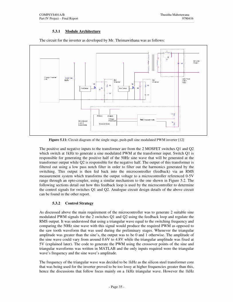
COMPSYS401A/B Thusitha Mabotuwana Part IV Project – Final Report 9790416
- Page 35 -
5.3.1 Module Architecture The circuit for the inverter as developed by Mr. Thrimawithana was as follows:
Figure 5.11: Circuit diagram of the single stage, push-pull sine modulated PWM inverter [12]
The positive and negative inputs to the transformer are from the 2 MOSFET switches Q1 and Q2 which switch at 1kHz to generate a sine modulated PWM at the transformer input. Switch Q1 is responsible for generating the positive half of the 50Hz sine wave that will be generated at the transformer output while Q2 is responsible for the negative half. The output of this transformer is filtered out using a low pass notch filter in order to filter out the harmonics generated by the switching. This output is then fed back into the microcontroller (feedback) via an RMS measurement system which transforms the output voltage to a microcontroller referenced 0-5V range through an opto-coupler, using a similar mechanism to the one shown in Figure 5.2. The following sections detail out how this feedback loop is used by the microcontroller to determine the control signals for switches Q1 and Q2. Analogue circuit design details of the above circuit can be found in the other report.
5.3.2 Control Strategy As discussed above the main requirement of the microcontroller was to generate 2 suitable sine modulated PWM signals for the 2 switches Q1 and Q2 using the feedback loop and regulate the RMS output. It was understood that using a triangular wave equal to the switching frequency and comparing the 50Hz sine wave with this signal would produce the required PWM as opposed to the saw tooth waveform that was used during the preliminary stages. Whenever the triangular amplitude was greater than the sine’s, the output was to be 0 and 1 otherwise. The amplitude of the sine wave could vary from around 0.6V to 4.8V while the triangular amplitude was fixed at 5V (explained later). The code to generate the PWM using the crossover points of the sine and triangular waveforms was written in MATLAB and the only inputs required were the triangular wave’s frequency and the sine wave’s amplitude. The frequency of the triangular wave was decided to be 1kHz as the silicon steel transformer core that was being used for the inverter proved to be too lossy at higher frequencies greater than this, hence the discussions that follow focus mainly on a 1kHz triangular wave. However the 1kHz

COMPSYS401A/B Thusitha Mabotuwana Part IV Project – Final Report 9790416
- Page 36 -
value could easily be changed in software to produce the required waveforms and PWM toggling points if required in the future. Figure 5.12 shows the output of MATLAB for a 1kHz triangular wave and a 4V sine wave. The PWM is shown in red.
Figure 5.12: Graph showing 50Hz sine, 1kHz triangular and output PWM when the 2 are compared. The above waveform shows a complete cycle of the 50Hz sine wave. However it can be seen that the PWM has a repeating pattern every half cycle (or every 10ms) of this waveform. The PWM corresponding to the first 10ms was to control switch Q1 and the one corresponding to 10ms-20ms was to control Q2. Q1 and Q2 were connected to 2 digital IO pins of the microcontroller and they were never to be ON (or logic high) at the same time. The PWM toggling points cannot be calculated on a runtime basis by the microcontroller since it needs a lot of processing. Therefore it was decided to store these points in Look-Up-Tables (LUT) in the microcontroller’s flash memory. However due to the repeating pattern of the PWM, only the points corresponding to half a cycle of the 50Hz wave (or 10ms) needed to be stored and the positive or negative half of the cycle could be accounted for in software. The required final waveform looked as in Figure 5.13.
Time(s)
V
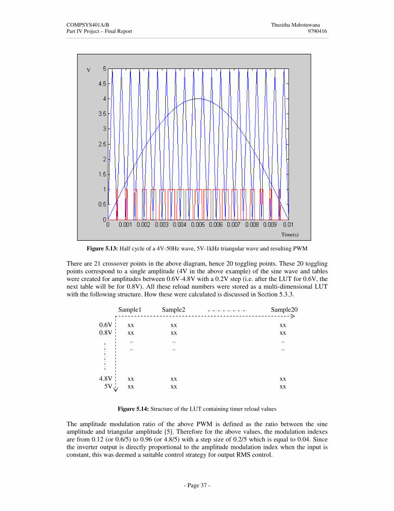
COMPSYS401A/B Thusitha Mabotuwana Part IV Project – Final Report 9790416
- Page 37 -
Figure 5.13: Half cycle of a 4V-50Hz wave, 5V-1kHz triangular wave and resulting PWM There are 21 crossover points in the above diagram, hence 20 toggling points. These 20 toggling points correspond to a single amplitude (4V in the above example) of the sine wave and tables were created for amplitudes between 0.6V-4.8V with a 0.2V step (i.e. after the LUT for 0.6V, the next table will be for 0.8V). All these reload numbers were stored as a multi-dimensional LUT with the following structure. How these were calculated is discussed in Section 5.3.3.
Sample1 Sample2 Sample20
0.6V xx xx xx 0.8V xx xx xx
.. .. .. .. .. ..
4.8V xx xx xx 5V xx xx xx
Figure 5.14: Structure of the LUT containing timer reload values The amplitude modulation ratio of the above PWM is defined as the ratio between the sine amplitude and triangular amplitude [5]. Therefore for the above values, the modulation indexes are from 0.12 (or 0.6/5) to 0.96 (or 4.8/5) with a step size of 0.2/5 which is equal to 0.04. Since the inverter output is directly proportional to the amplitude modulation index when the input is constant, this was deemed a suitable control strategy for output RMS control.
Time(s)
V

COMPSYS401A/B Thusitha Mabotuwana Part IV Project – Final Report 9790416
- Page 38 -
The complete control strategy for the inverter is given in the flowchart shown in Figure 5.15.
Figure 5.15: Flowchart showing how output regulation is achieved As discussed above the LUTs are generated for various modulation indexes. The idea behind the regulation scheme that has been implemented is to simply update the current PWM to compensate for the output change. For example, if the output increases by 5V, in the next cycle of the 50Hz wave the PWM will be updated such that the new PWM would generate an output wave of 5 less than the previous.
Yes
No All caps initialised?
ADC source?
Process as in Figure 5.6
Calculate: NOMINAL - feedback
Set next ADC channel
Feedback channel and flag: checkFeedback=1
Supercapacitor bank
Determine PWM LUT that would compensate for the change
Set LUT_index to load timer with this LUT and flag:checkFeedback=0
Reset
Main loop (Stay infinitely)
Interrupt
Read ADC value
ADC
System Initialisation
timer0
Load timer with next reload number using LUT_index
and sample number
Cycle (+ve or –ve?)
+ve -ve
Generate control for Q1
Generate control for Q2
Update sample number
If end of complete cycle, update +ve or -ve
If middle of half cycle, set flag: checkFeedback=1

COMPSYS401A/B Thusitha Mabotuwana Part IV Project – Final Report 9790416
- Page 39 -
5.3.3 Timing Issues timer0 of the microcontroller was used to generate the required PWM timing. It was to generate a timer interrupt based on the above calculated toggling points. Section 4.2.3 explained how the reload number for this timer could be calculated, and the same calculation was performed in MATLAB to output the final timer-reload values. For example for the above graph, MATLAB would give the timer-reload values in the following format.
Figure 5.16: Command window output of MATLAB showing timer0 reload values The timer was running with a 4µs period and the number 64 at the very beginning means that timer0 should be reloaded with the value 64 to produce a timer interrupt of 4µs x 64 = 256µs, which is also the point where the PWM changes its values from 0 to 1 as shown in Figure 5.13. Other timer interrupt values can also be calculated in a similar manner. As previously discussed the feedback loop was implemented to regulate the RMS output. A very fast transient response was not expected from the system and it was deemed that regulating the output once per half cycle (i.e. every 10ms) was adequate. Therefore the flag checkFeedback shown in the flowchart is set only every 10 samples.
5.3.4 Output and Regulation Load regulation characteristics and line regulation characteristics of the inverter were measured to determine the performance of the system. Using a power analyser the output voltage and current were measured along with total harmonic distortion (THD) for various load and values tabulated as shown in Table 5.1.
Power (W) Output V (per unit) THD % I (A)
4 0.992 15 0.034 5.5 1 14 0.04 8.5 0.96 14.2 0.073 10 0.988 12.9 0.079
13.7 0.986 13.9 0.11 15.5 0.992 13.7 0.13 20 0.99872 13.6 0.16
21.2 1.008 13.5 0.17 21 0.96 13.9 0.18 27 1 13.6 0.21
27.3 0.96 13.8 0.23 30 0.84 15.6 0.28
Table 5.1: Output regulation parameters

COMPSYS401A/B Thusitha Mabotuwana Part IV Project – Final Report 9790416
- Page 40 -
Nominal voltage was taken as 110Vrms mainly due to transformer issues discussed in previous sections. Based on this value output voltage was also calculated on a per unit basis. Figure 5.17 shows the graphs plotted from the above data.
Figure 5.17: Output voltage regulation: (left) Output Vrms Vs. Load (right) Output V(per unit) Vs. Load
5.4 System Integration As discussed in previous sections, the first module that was developed was the charge transfer unit. After testing the circuits on bred-board it was decided to build PCBs so that we could test this module using both, the analogue and digital interfaces. Proper testing could not be done with the circuits on bred-board since they can support only limited amount of current. Shown in Figure 5.18(bottom) is a photograph of the first set of PCBs that were made for the charge transfer unit along with the commercial inverter that was purchased. Figure 5.18(top) shows the microcontroller extension board that was used to interface to these banks. The schematic of this extension board is included in Appendix C..
Figure 5.18: Photographs showing (top) microcontroller and extension board (bottom) charge transfer unit PCBs and commercial inverter
Microcontroller extension board
STK500 development board
Atmel Mega8535 microcontroller
One of the 3 banks in the charge transfer unit
Commercial inverter that was being used

COMPSYS401A/B Thusitha Mabotuwana Part IV Project – Final Report 9790416
- Page 41 -
The microcontroller extension board was made to provide an interface to ADC/digital input, VCC, ground and analogue comparator input each supercapacitor module contains. This board was designed to support up to 8 such modules, although only 3 were being used by the current scheme. Testing of the system proved that the analogue ADC method was better than the digital interface and this was described in detail in Section 4.2.2. Therefore the system was tested with the analogue interface connections from here on. The next stage of the development included developing the inverter. After this was sufficiently developed and tested using techniques discussed in previous sections, the commercial inverter was replaced with this unit. The charger module was developed as the last stage of the integration process and the complete system was tested to verify system behaviour. Finally on suggestion of our supervisor it was decided to build the final PCBs where each supercapacitor bank was to function as a plug-in unit on a main-board. Each bank was made as compact as possible and looked as shown below.
(a) (b) Figure 5.19: A final supercapacitor bank with plug-in feature (a) top view (b) bottom view
This plug-in feature allows the users to easily replace any destroyed or non-functional units, hence providing a user-friendly functionality. At the time of writing this report the main-board has not been completely soldered, but the completed final system would look similar to the one shown in Figure 5.20. This board’s schematic is given in Appendix D.
Figure 5.20: Projected final system view (transformer not shown)
Self-contained supercapacitor banks
Output
Input Inverter circuitry
Energy pump circuitry
Microcontroller subsystem

COMPSYS401A/B Thusitha Mabotuwana Part IV Project – Final Report 9790416
- Page 42 -
Shown below in Figure 5.21 is a block diagram of the microcontroller showing all its inputs and outputs along with the corresponding pins used.
Figure 5.21: System inputs and outputs to and from the microcontroller
Microcontroller (Atmel Mega8535)
ADC0
ADC1
ADC2
PORTB.0
PORTB.1
PORTB.2
PORTC.0
PORTC.2
PORTC.1
Bank0 voltage Bank1 voltage Bank2 voltage
Control logic for charge transfer unit
Inputs from charge transfer unit
ADC3 Output voltage PORTD.6
PORTD.7
Bank0 charging logic Bank1 charging logic Bank2 charging logic Bank0 discharging logic Bank1 discharging logic Bank2 discharging logic
PWM control for Q1 PWM control for Q2 Control for inverter
switches Q1 and Q2
Inverter feedback
Over voltage logic Over current logic
PORTD.0
PORTD.2 (Ext. Int)
PORTD.3
PWM control for charging switch
Control for energy pump
Inputs from energy pump

COMPSYS401A/B Thusitha Mabotuwana Part IV Project – Final Report 9790416
- Page 43 -
A final flowchart showing the required control for the fully integrated system is shown below in Figure 5.22.
Figure 5.22: Flowchart showing control provided for the final system
Yes
No All caps initialised?
ADC source?
Process as in Figure 5.6
Calculate: NOMINAL - feedback
Set next ADC channel
Feedback channel and flag: checkFeedback=1 Supercapacitor
bank
Determine PWM LUT that would compensate
for the change
Set LUT_index to load timer with this LUT and flag:checkFeedback=0
Reset
Main loop (Stay infinitely)
Interrupt
Read ADC value
ADC
System Initialisation
timer0 overflow
Load timer with next reload number using LUT_index
and sample number
Cycle (+ve or –ve?)
+ve -ve
Generate control for
Q1
Generate control for
Q2
Update sample number
If end of complete cycle, update +ve or -ve
If middle of half cycle, set flag: checkFeedback=1
external timer2 overflow
Make output 0 instead of PWM Over
voltage condition
Generate PWM by writing 1 or 0 to pin
False
True
Make output 0 instead of PWM

COMPSYS401A/B Thusitha Mabotuwana Part IV Project – Final Report 9790416
- Page 44 -
5.5 Cost Analysis A cost analysis was carried out for the developed system and details are shown in Table 5.2. The final cost can be reduced to around NZ$130 if produced on a mass scale.
Component Cost (NZ$) Per unit price
Cost (NZ$) Per 10000 units price
Transformers 120.00 40.00 Supercapacitors 120.00 30.00 Microcontroller 20.00 5.00
Other components (FETs, Opto-couplers etc) 120.00 55.00
Total Cost (approximately) 380.00 130.00 Table 5.2: Cost analysis of the developed system

COMPSYS401A/B Thusitha Mabotuwana Part IV Project – Final Report 9790416
- Page 45 -
6.0 Suggested Future Developments The system that has been implemented was developed mainly as a proof of concept design and therefore aspects such as optimisation, efficiency and cost minimisation were not considered of high priority. Although the basic concepts and algorithms of the developed system can be used for future work, we would like propose some future enhancements that can be added to improve the quality of the complete system.
• Consider using cheaper supercapacitors with higher capacitance, and if possible lower ESR. This will lower the cost of the system and also minimise losses.
• Optimise the inverter module by considering other implementation techniques. Also higher switching frequencies can be looked at which in turn will make the filter design easier.
• Improve the performance of the energy pump. • Include redundancy of supercapacitor banks and program the controller to check for any
destroyed or non-functional banks. This can easily be done by turning a timer ON as soon as a bank is set to CHARGING mode. If the bank does not reach the fully-charged condition within the pre-defined time (say 20ms), generate a timeout and deem the bank was faulty. timer1 even of the existing processor can be used for this purpose.
• Design a user interface to show current system status and a log of surges the system might have encountered. Details can easily be retained by writing to EEPROM memory of the microcontroller which will retain data even after a system reset.
• Test the system with a surge simulator and evaluate performance. An external interrupt can be used to detect a transient condition and within this interrupt routine, different input pins can be read to determine a range for the surge. For example if 5 pins were allocated for range determination and if 00011 was read the range can be between 400-600V and if 00111 was read the range is between 600-800V and so on.
• Consider a compact FPGA or DSP implementation. Using an FPGA will be cost effective since this can be fully customised. A DSP implementation can be used if complex algorithms are to be implemented and if software filters and other signal processing aspects are required.
• Finally with the above features implemented a commercial prototype can be developed. 7.0 Conclusions A complete system with an energy pump, charge transfer unit, an inverter and a microcontroller subsystem has successfully been implemented. The possibility of dynamic energy transfer using supercapacitors was investigated during the course of the project and was proven to be feasible with experimental results. This dynamic energy transfer always provides complete input-output isolation, hence common and differential mode surge protection. A 15kHz, 40% duty cycle PWM has been used to control the energy pump with over voltage and current protection. The charge transfer unit consists of three 0.2F/18V supercapacitor banks that dynamically transfer energy to the inverter while providing the required isolation. The inverter is controlled using a 1kHz sine modulated PWM scheme with approximately 4% output voltage regulation. Microcontroller that was used was an Atmel Mega8535 and the complete system is valued at approximately NZ$380.

COMPSYS401A/B Thusitha Mabotuwana Part IV Project – Final Report 9790416
- Page 46 -
References 1. Kularatna, N. (1998) Power Electronics Handbook: Low-Power Components and
Application. Boston, Newnes. 2. Patel, N. (2004) Introduction to Projects. Lecture handout, COMPSYS401: Part IV Project,
University of Auckland. 3. In Search of Quality Power. Retrieved 30 March, 2004 from
http://www.advancedenergy.org/progressenergy/powerquality.html 4. Uninterrupted Power Supply (UPS) Systems. Retrieved 28 March, 2004 from
http://www.io.com/~hcexres/tcm1603/acchtml/recomx5c.html 5. Mohan, N., Undeland, T.M. and Robbins, W.P. (1989) Power electronics: converters,
applications and design. 1st edition, Wiley, New York. 6. Standby UPS / Standby Power Supply. Retrieved 05 April, 2004 from
http://www.pcguide.com/ref/power/ext/ups/typesStandby-c.html 7. Supercapacitor Properties. Retrieved 10 April, 2004 from
http://www.cooperet.com/pdfs_html/PowerStorProductOverview.pdf 8. Nek Tockin Corporation. Retrieved March 20, 2004, from http://www.nec-tokin.com/english/ 9. Thrimawithana, D.J. (2004) Interim Report. ELECTENG 401A/B Project, School of
Engineering, University of Auckland. 10. Mabotuwana, T., (2004) Interim Report. ELECTENG 401A/B Project, School of
Engineering, University of Auckland. 11. Atmel 90S8535. Retrieved 29 March, 2004 from
http://www.avrfreaks.net/Devices/devices.php?action=1&devid=11 12. Thrimawithana, D.J. (2004) Final Report. ELECTENG 401A/B Project, School of
Engineering, University of Auckland. 13. Atmel Mega8535. Retrieved 15 May, 2004 from
http://www.avrfreaks.net/Devices/devices.php?action=1&devid=65 14. 74HC/HCT02; Quad 2-input NOR gate. Retrieved 20 June, 2004 from
http://www.semiconductors.philips.com/pip/74HC02.html 15. Buyukbozkirli, B. and Chrifi-Alaoui, H. (2001) An Alternative Pulse-Width Modulation
Scheme for Automotive Inverters. Michigan State University. 16. ANSI/IEEE C62.41, 1980. IEEE Guide for Surge Voltages in Low-Voltage AC Power
Circuits, Institue of Electrical and Electronics Engineers, New York. 17. M68HC08 Family. Retrieved 30 March, 2004 from
http://e-www.motorola.com/webapp/sps/site/taxonomy.jsp?nodeId=01624684498634 18. Atmel Corporation: AVR 8-Bit RISC. Retrieved 30 March, 2004 from
http://www.atmel.com/dyn/products/param_table.asp?family_id=607&OrderBy=part_no&Direction=ASC
19. Microchip Products. Retrieved 29 March, 2004 from http://www.microchip.com/ParamChartSearch/chart.aspx?branchID=1095&mid=&lang=en&pageId=74

COMPSYS401A/B Thusitha Mabotuwana Part IV Project – Final Report 9790416
- Page 47 -
Bibliography Barnett , R., O'Cull, L. and Cox S. (2002) Embedded C programming and the Atmel AVR. Clifton Park, New York. Kularatna, N. (2000) Modern Component Families and Circuit Block Design. Boston, Newnes. IEEE Power Engineering Society, C62.41.1, 2002. IEEE Guide for Surge Voltages in Low-Voltage (1000V and Less) AC Power Circuits, Institue of Electrical and Electronics Engineers, New York. IEEE Power Engineering Society, C62.41, 1991. IEEE recommended Practice on Surge Voltages in Low-Voltage AC Power Circuits, Institue of Electrical and Electronics Engineers, New York. Microcontroller Links. 20 March, 2004 from http://digital5.ece.tntech.edu/TechLinks/mc_links.htm Haykin, S.S. (2001) Communication Systems. 4th edition, Wiley, New York. Microcontroller. Retrieved 30 March, 2004 from http://members.ozemail.com.au/~mvw/micro.html Sedra, S.A. and Smith, K.C. (1998) Microelectronic circuits. 4th edition, Oxford University Press, New York.

COMPSYS401A/B Thusitha Mabotuwana Part IV Project – Final Report 9790416
- Page i -
Appendices
Appendix A: Extract from IEEE C62.41 Class B Standard ........................................................... ii
Appendix B: Selection Process for a Suitable Microcontroller .................................................... iv
Appendix C: Schematic of the Microcontroller Extension Board ................................................ vi
Appendix D: Schematic of the Main-Board................................................................................. vii
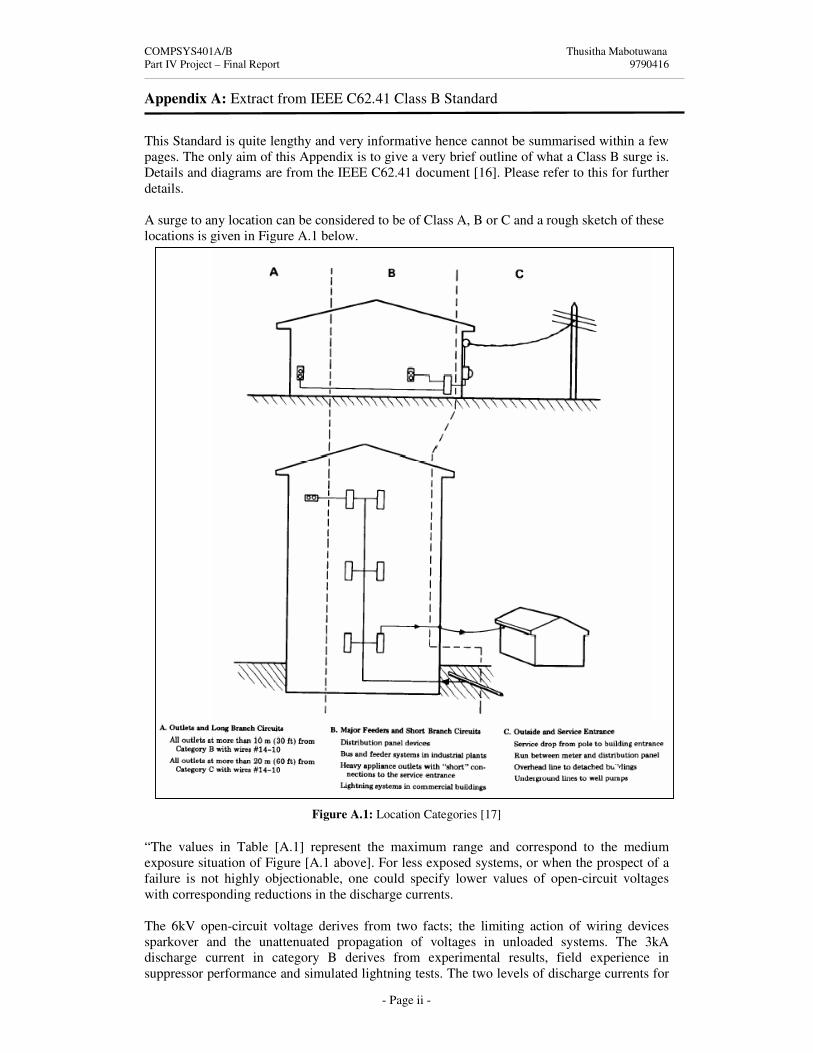
COMPSYS401A/B Thusitha Mabotuwana Part IV Project – Final Report 9790416
- Page ii -
Appendix A: Extract from IEEE C62.41 Class B Standard
This Standard is quite lengthy and very informative hence cannot be summarised within a few pages. The only aim of this Appendix is to give a very brief outline of what a Class B surge is. Details and diagrams are from the IEEE C62.41 document [16]. Please refer to this for further details. A surge to any location can be considered to be of Class A, B or C and a rough sketch of these locations is given in Figure A.1 below.
Figure A.1: Location Categories [17] “The values in Table [A.1] represent the maximum range and correspond to the medium exposure situation of Figure [A.1 above]. For less exposed systems, or when the prospect of a failure is not highly objectionable, one could specify lower values of open-circuit voltages with corresponding reductions in the discharge currents. The 6kV open-circuit voltage derives from two facts; the limiting action of wiring devices sparkover and the unattenuated propagation of voltages in unloaded systems. The 3kA discharge current in category B derives from experimental results, field experience in suppressor performance and simulated lightning tests. The two levels of discharge currents for

COMPSYS401A/B Thusitha Mabotuwana Part IV Project – Final Report 9790416
- Page iii -
the 0.5 microsecond-100kHz wave derive from the increasing impedance expected in moving from location B to location A. Location C is likely to be exposed to substantially higher voltages than location B because the limiting effect of sparkover is not available. The high-exposure rates of Table [A.1] could apply with voltage in excess of 10kV and discharge currents of 10kA or more. Installing unprotected load equipment in location C is not recommended; the installation of secondary arresters however can provide the necessary protection. Secondary arresters having 10kA ratings have been applied successfully for many years in location C” [10].
Table A.1: Surge voltages and currents at standard locations [17]

COMPSYS401A/B Thusitha Mabotuwana Part IV Project – Final Report 9790416
- Page iv -
Appendix B: Selection Process for a Suitable Microcontroller Based on circuits that were designed during the initial stages of the project, the control signals for the overall system were as shown in Table B.1. Please refer to the interim reports for a details analysis of these figures.
Purpose Input and Outputs
Monitor line voltages 1 A/D input 4-8 inputs from the ladder circuitry
Monitor bank voltage 1 A/D pin for each bank x number of banks = 5 (assuming 5 banks)
Battery health 1 A/D pin Monitor output 1 A/D pin
Control for banks 4 output pins for each bank x number of banks = 20 (assuming 5 banks)
Control for supercapacitor charger 1 pin Control for battery charger 1 pin Control for inverter 3 pins Total I/O lines required Around 40
Table B.1: Total I/Os required by the microcontroller As shown in above table, we needed a total of approximately 40 I/O lines. This requirement was given the highest priority in the selection process. Apart from this, the following were considered: - 16MHz or higher to provide fast processing - Needed a simple 8-bit controller since we haven’t got much data movement - A UART to interface with a PC (this was to be done only if time-permitted but still needed
to be accounted for) - Around 6 A/D channels – 4 for the supercapacitor banks and 1 for output feedback. - Approximately 16kB flash memory. Better to have more to be on the safe side. - Intended to use a 5V microcontroller since most of the electronic components which
would be used were 5V. - Around1kB of SRAM for variables and other storage. - At least 1 external interrupt to capture transient conditions. - Around 3 timers to detect the duration of a surge and also for other timeouts (for example
to detect a bank taking too long to charge, due to a fault). - Watchdog timer to monitor the system and recover if something went wrong. - Use minimum power as possible For this project it was decided to use a microcontroller instead of a DSP or an FPGA mainly due to the following reasons: - We were not trying to develop a surge measurement system, so there was no need to
determine the actual value of the surge. A range such as 500-1000V, 1000-1500V was sufficient, which could be measured by using an external interrupt with a few IO pins which would correspond to various ranges. Therefore there was no need for very high sampling rates.
- The cost of a DSP system is very high compared to a microcontroller and did not help in minimising cost of the product.
- A microcontroller could be used to accomplish all the required tasks of the controller subsystem except for measuring an exact value for a high voltage transient.
- I have no prior experience working with a DSP system and difficulty of properly learning such a system within the given time constraint.
- There were many new concepts that were being tried out where quick control programs had to be written. The development process is much faster with microcontroller compared to FPGA.
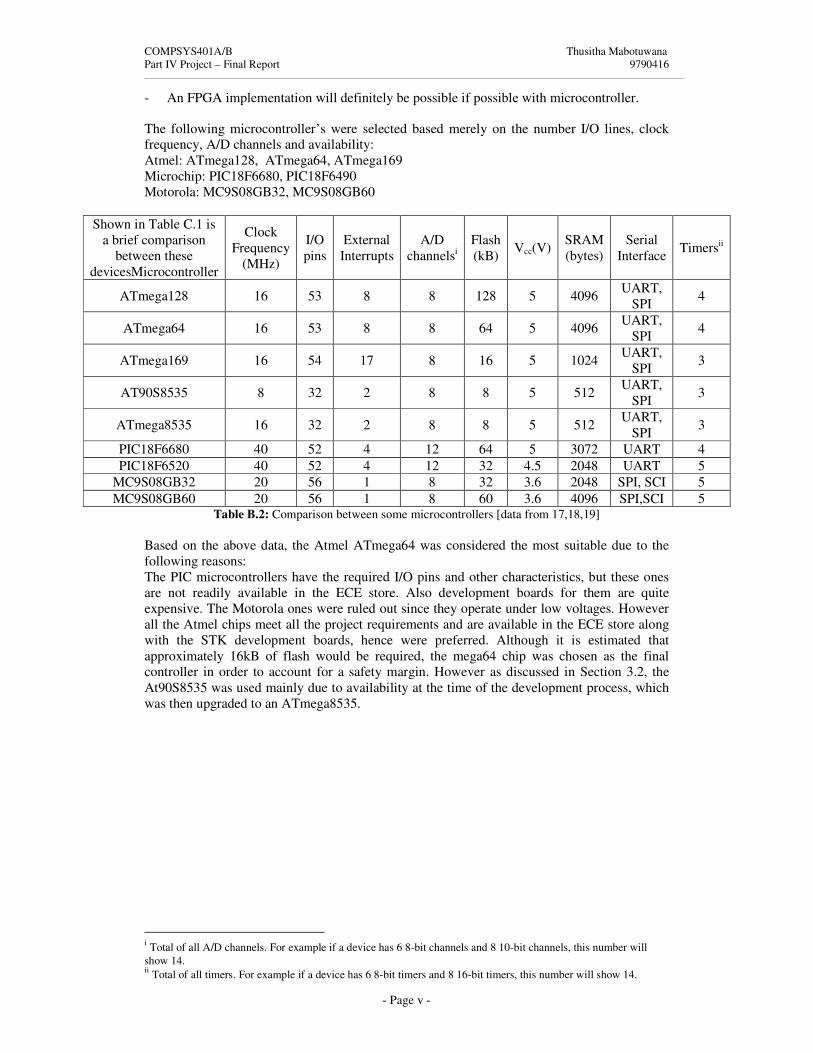
COMPSYS401A/B Thusitha Mabotuwana Part IV Project – Final Report 9790416
- Page v -
- An FPGA implementation will definitely be possible if possible with microcontroller. The following microcontroller’s were selected based merely on the number I/O lines, clock frequency, A/D channels and availability: Atmel: ATmega128, ATmega64, ATmega169 Microchip: PIC18F6680, PIC18F6490 Motorola: MC9S08GB32, MC9S08GB60
Shown in Table C.1 is a brief comparison
between these devicesMicrocontroller
Clock Frequency
(MHz)
I/O pins
External Interrupts
A/D channelsi
Flash (kB) Vcc(V) SRAM
(bytes) Serial
Interface Timersii
ATmega128 16 53 8 8 128 5 4096 UART, SPI 4
ATmega64 16 53 8 8 64 5 4096 UART, SPI 4
ATmega169 16 54 17 8 16 5 1024 UART, SPI 3
AT90S8535 8 32 2 8 8 5 512 UART, SPI 3
ATmega8535 16 32 2 8 8 5 512 UART, SPI 3
PIC18F6680 40 52 4 12 64 5 3072 UART 4 PIC18F6520 40 52 4 12 32 4.5 2048 UART 5
MC9S08GB32 20 56 1 8 32 3.6 2048 SPI, SCI 5 MC9S08GB60 20 56 1 8 60 3.6 4096 SPI,SCI 5
Table B.2: Comparison between some microcontrollers [data from 17,18,19] Based on the above data, the Atmel ATmega64 was considered the most suitable due to the following reasons: The PIC microcontrollers have the required I/O pins and other characteristics, but these ones are not readily available in the ECE store. Also development boards for them are quite expensive. The Motorola ones were ruled out since they operate under low voltages. However all the Atmel chips meet all the project requirements and are available in the ECE store along with the STK development boards, hence were preferred. Although it is estimated that approximately 16kB of flash would be required, the mega64 chip was chosen as the final controller in order to account for a safety margin. However as discussed in Section 3.2, the At90S8535 was used mainly due to availability at the time of the development process, which was then upgraded to an ATmega8535.
i Total of all A/D channels. For example if a device has 6 8-bit channels and 8 10-bit channels, this number will show 14. ii Total of all timers. For example if a device has 6 8-bit timers and 8 16-bit timers, this number will show 14.

COMPSYS401A/B Thusitha Mabotuwana Part IV Project – Final Report 9790416
- Page vi -
Appendix C: Schematic of the Microcontroller Extension Board The above PCB was designed to support up to 8 complete supercapacitor banks although only 3 were being used in the current design.
Title
NumberSize
A4
VCC
1 23 45 67 8GND VCC
ANLG_PORT
ANLG_PORT
1 23 45 67 8GND VCC
CHRGN_PORT
CHRGN_PORT
1 23 45 67 8GND VCC
DISCHRGN_PORT
DISCHRGN_PORT
1_O VCC1a 4_O1b 4b2_O 4a2a 3_O2b 3bGND 3a
NOR1
74HCT02N_1
1_O VCC1a 4_O1b 4b2_O 4a2a 3_O2b 3bGND 3a
NOR2
74HCT02N_2
CD
BANK1
BANK1
CD
BANK2
BANK2
CD
BANK3
BANK3
CD
BANK4
BANK4
CD
BANK5
BANK5
CD
BANK6
BANK6
CD
BANK7
BANK7
CD
BANK8
BANK8
VCCAorDCMPGND
JP1
BANK1
VCCAorDCMPGND
JP2
BANK2
VCCAorDCMPGND
JP3
BANK3
VCCAorDCMPGND
JP4
BANK4
VCCAorDCMPGND
JP5
BANK5
VCCAorDCMPGND
JP6
BANK6
VCCAorDCMPGND
JP7
BANK7
VCCAorDCMPGND
JP8
BANK8
VCC
VCC
VCC
VCC
VCC
VCC
VCC
GND
GND
GND
GND
GND
GND
GND
GND
VCC
GND
GND VCC
GND
VCC
GND VCC
AorD1
AorD2
AorD3
AorD4
AorD5
AorD6
AorD7
AorD8
AorD1 AorD2AorD3 AorD4AorD5 AorD6AorD7 AorD8GND VCC
Cout1
Cout2
Cout3
Cout4
Cout5
Cout6
Cout7
Cout8
Cout1
Cout2Cout3
Cout4
Cout5
Cout6Cout7
Cout8
Dout1 Dout2Dout3 Dout4Dout5 Dout6Dout7 Dout8
Dout2
Dout3
Dout4
Dout5
Dout6
Dout7
Dout8
Dout1CMP1
CMP2
CMP3
CMP4
CMP5
CMP6
CMP7
CMP8
CMP1
CMP2
CMP3
CMP4
CMP5
CMP6
CMP7
CMP8
CH1 CH2CH3 CH4CH5 CH6CH7 CH8
CH1
CH2 CH3
CH4
CH5
CH6 CH7
CH8
Inputs to the microcontroller from charge transfer unit
Control signals from the microcontroller to charge transfer unit

COMPSYS401A/B Thusitha Mabotuwana Part IV Project – Final Report 9790416
- Page vii -
1 2 3 4 5 6
A
B
C
D
654321
D
C
B
A
Title
Number RevisionSize
C
Date: 12-Sep-2004 Sheet of File: P:\50-59\57\PCB3\MotherBoard.Ddb Drawn By:
Q4MOSFET N D21
DIODE
D22DIODE
D16DIODE
D18DIODE
D17DIODE
D19DIODE
12
J3
CON2
C14CAPACITOR
C21CAP
R25RES1
12
J4
CON2
D23
DIODE
C15
CAPACITOR
U7OPTOISO2
15
26
37
48 MC34152
HEADER 4X2
R24RES1
12
JP8HEADER 2
C22CAP
C16
CAPACITOR
R29
RES1
R30RES1
12
3
4
5
67
8
1
1
REF
U5
MAX951
Vu_5V
GND_U
R31RES1
R32RES1
GND_U
R26RES1
12345
ACS752HEADER 5
Vu_5V
GND_U
GND_UPD2
PD0
U6
OPTOISO2
D30 ZENER3
D31ZENER3R27
RES1
Vu_5V
GND_U
R28RES1
PD3
Q5MOSFET N
Q6MOSFET NR36
RES1
R40
RES1
D26DIODE
C23
CAP
R39RES1
R41RES1
C27
CAP
D27DIODE
15
26
37
48 MC34152
HEADER 4X2
CapOut+
GND_U
C17
CAPACITORC24CAP
R37
RES1
R38
RES1
PD6
PD7
R33RES1
12
JP9HEADER 2 R34
RES1
R42RES1
R43RES1
D24DIODE
D28DIODE
D25DIODE
D29DIODE
C28CAP
C18CAPACITOR
R35RES1
U8OPTOISO2
R44RES1
GND_U
Vu_5V
R22RES1
R23RES1
C19CAP
C20CAP
D20DIODE
CapCharge+
1 23 45 67 89 1011 1213 1415 1617 1819 2021 2223 2425 2627 2829 3031 3233 3435 3637 3839 4041 4243 4445 4647 4849 50
JP12HEADER 25X2 1 2
3 45 67 89 1011 1213 1415 1617 1819 2021 2223 2425 2627 2829 3031 3233 3435 3637 3839 4041 4243 4445 4647 4849 50
JP13HEADER 25X21 2
3 45 67 89 1011 1213 1415 1617 1819 2021 2223 2425 2627 2829 3031 3233 3435 3637 3839 4041 4243 4445 4647 4849 50
JP11HEADER 25X2 1 2
3 45 67 89 1011 1213 1415 1617 1819 2021 2223 2425 2627 2829 3031 3233 3435 3637 3839 4041 4243 4445 4647 4849 50
JP14HEADER 25X2
CapCharge+
CapCharge-
CapOut+
GND_U
Vu_5V
CapCharge-
ADC1PB0PC0GND_UTest0+Test0-
ADC2PB1PC1
Test1+Test1-
ADC3PB2PC2
Test2+Test2-
ADC4PB3PC3
Test3+Test3-
1 23 45 67 89 10
JP19HEADER 5X2
1 23 45 67 89 10
JP20
HEADER 5X2
1 23 45 67 89 10
JP30
HEADER 5X2
1 23 45 67 89 10
JP18
HEADER 5X2
ADC0 ADC1ADC3ADC2
PB0PB2
PB1PB3
PC0PC2
PC1PC3
PD0PD2
PD6
PD3
PD7Vu_5V GND_U
1234
JP17
HEADER 4
1234
JP7
4 HEADER
XTAL2XTAL1
RESET
GND_UVu_5V GND_U
1 402 393 384 375 366 357 348 339 3210 3111 3012 2913 2814 2715 2616 2517 2418 2319 2220 21
Mega1
HEADER 20X2
PB0PB1PB2PB3PB4
PD2PD3PD4PD5PD6 PD7
PC0PC1PC2PC3PC4PC5PC6PC7
ADC0ADC1ADC2ADC3ADC4ADC5ADC6ADC7AREF
PB5PB6PB7
X216Mhz
C3327pf
C3427pf
C35
100nF
SW2
SW-PB
GND_U
GND_U
GND_U
RESET
R48
10k
XTAL2XTAL1
Vu_5V
GND_U
D34
LED
R47
270
Vu_5V
+ C29
220uF
+ C30
220uF321J5
DCJACK
Vin1
GN
D2
Vout 3U9
LM7805
+12VD33
1N4007+ C32
1uF TANC31CER
Vu_5V
PD0PD1
ADC0
ADC4
Appendix D: Schematic of the Main-Board
Microcontroller Power Supply
Mega8535 Microcontroller
PCI slots for supercapacitor banks
Energy Pump - input Energy Pump - output
Inverter - input
Inverter - output
Microcontroller Connections