An efficient way to learn deep generative models

Geoffrey HintonCanadian Institute for Advanced Research

&Department of Computer Science

University of Toronto

Joint work with: Ruslan Salakhutdinov, Yee-Whye Teh, Simon Osindero, Ilya Sutskever,

Graham Taylor, Andriy Mnih

Belief Nets

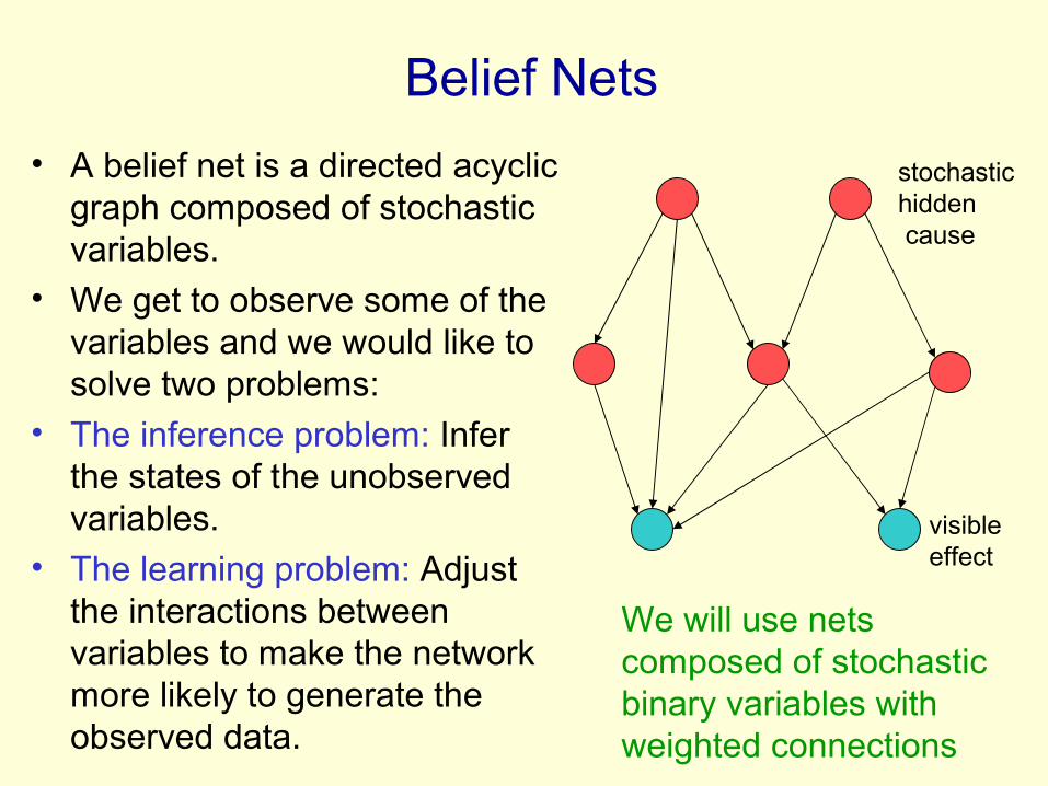
• A belief net is a directed acyclic graph composed of stochastic variables.

• We get to observe some of the variables and we would like to solve two problems:

• The inference problem: Infer the states of the unobserved variables.

• The learning problem: Adjust the interactions between variables to make the network more likely to generate the observed data.

stochastichidden cause

visible effect

We will use nets composed of stochastic binary variables with weighted connections

Stochastic binary neurons

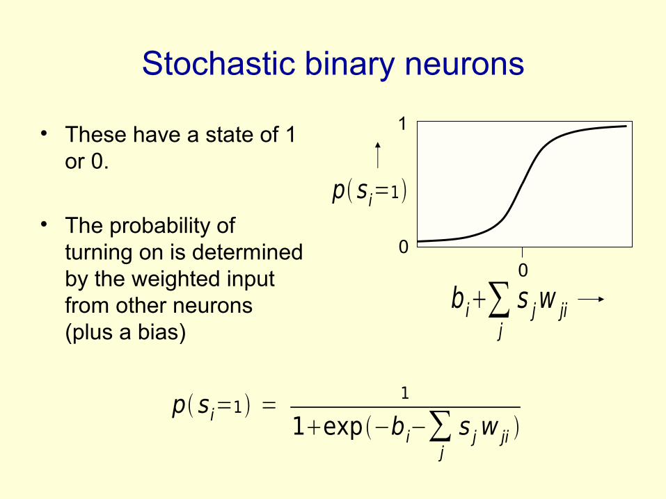
• These have a state of 1 or 0.

• The probability of turning on is determined by the weighted input from other neurons (plus a bias)

00

1

p si=1 =1

1exp −bi−∑js jw ji

bi∑j

s jw ji

p si=1

Learning Belief Nets

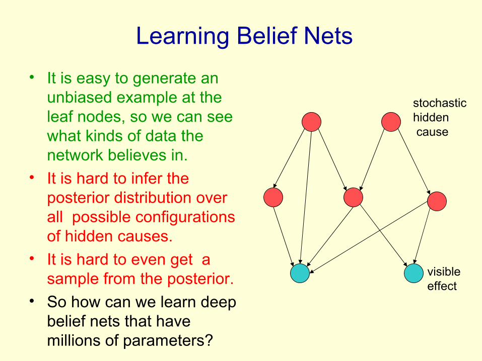
• It is easy to generate an unbiased example at the leaf nodes, so we can see what kinds of data the network believes in.

• It is hard to infer the posterior distribution over all possible configurations of hidden causes.

• It is hard to even get a sample from the posterior.

• So how can we learn deep belief nets that have millions of parameters?

stochastichidden cause

visible effect

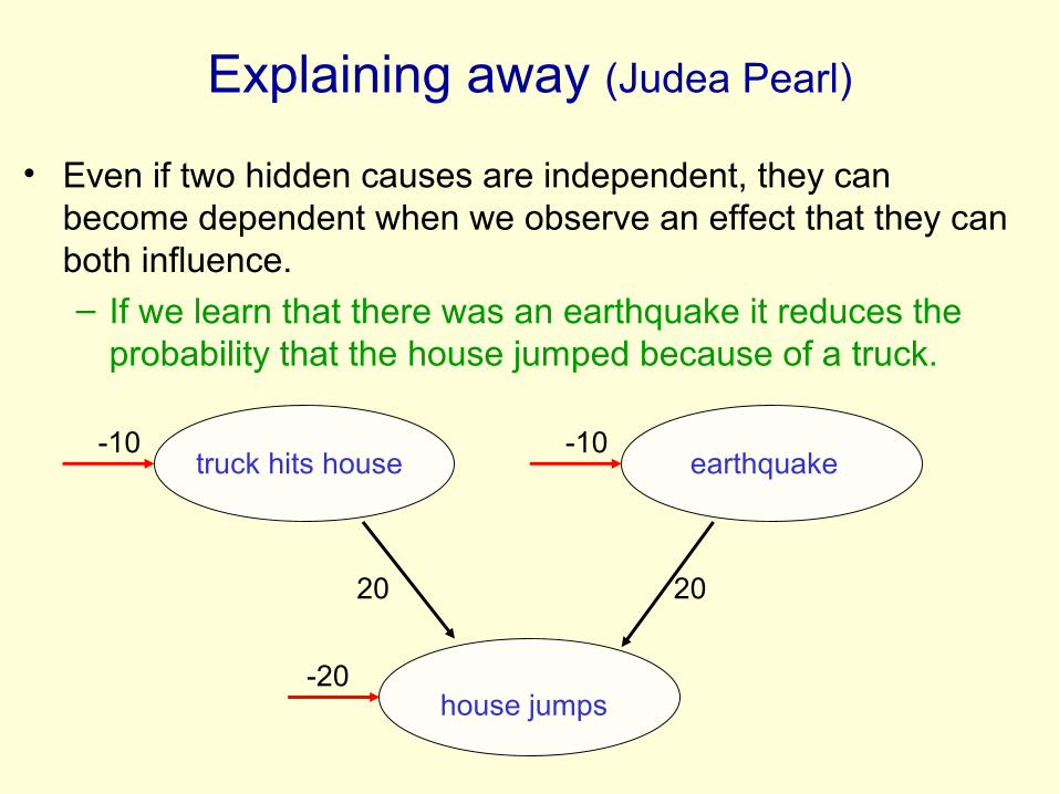
Explaining away (Judea Pearl)

• Even if two hidden causes are independent, they can become dependent when we observe an effect that they can both influence. – If we learn that there was an earthquake it reduces the

probability that the house jumped because of a truck.

truck hits house earthquake

house jumps

20 20

-20

-10 -10

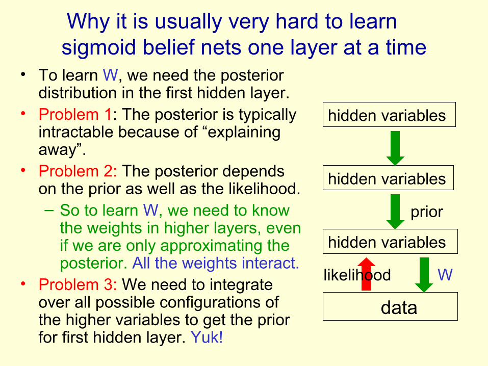
Why it is usually very hard to learn sigmoid belief nets one layer at a time

• To learn W, we need the posterior distribution in the first hidden layer.

• Problem 1: The posterior is typically intractable because of “explaining away”.

• Problem 2: The posterior depends on the prior as well as the likelihood. – So to learn W, we need to know

the weights in higher layers, even if we are only approximating the posterior. All the weights interact.

• Problem 3: We need to integrate over all possible configurations of the higher variables to get the prior for first hidden layer. Yuk!

data

hidden variables

hidden variables

hidden variables

likelihood W

prior

Two types of generative neural network

• If we connect binary stochastic neurons in a directed acyclic graph we get a Sigmoid Belief Net (Radford Neal 1992).

• If we connect binary stochastic neurons using symmetric connections we get a Boltzmann Machine (Hinton & Sejnowski, 1983).– If we restrict the connectivity in a special way,

it is easy to learn a Boltzmann machine.

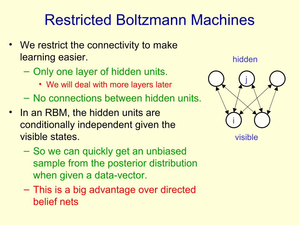
Restricted Boltzmann Machines

• We restrict the connectivity to make learning easier.– Only one layer of hidden units.

• We will deal with more layers later

– No connections between hidden units.• In an RBM, the hidden units are

conditionally independent given the visible states.

– So we can quickly get an unbiased sample from the posterior distribution when given a data-vector.

– This is a big advantage over directed belief nets

hidden

i

j

visible

Weights Energies Probabilities

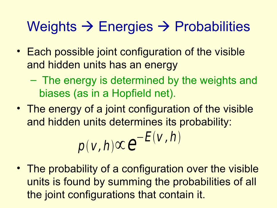
• Each possible joint configuration of the visible and hidden units has an energy– The energy is determined by the weights and

biases (as in a Hopfield net).• The energy of a joint configuration of the visible

and hidden units determines its probability:

• The probability of a configuration over the visible units is found by summing the probabilities of all the joint configurations that contain it.

p v ,h ∝e−E v ,h

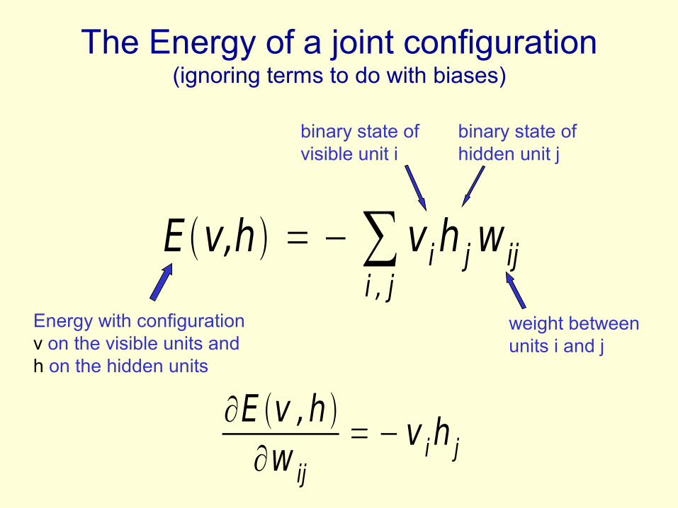
The Energy of a joint configuration(ignoring terms to do with biases)

E v,h = − ∑i , j

vih jw ij

weight between units i and j

Energy with configuration v on the visible units and h on the hidden units

binary state of visible unit i

binary state of hidden unit j

∂E v ,h ∂w ij

= − v ih j

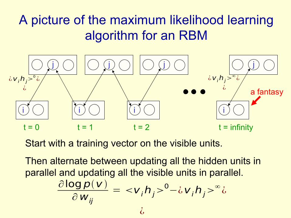
A picture of the maximum likelihood learning algorithm for an RBM

¿v ih j0¿

¿

¿v ih j∞¿

¿

i

j

i

j

i

j

i

j

t = 0 t = 1 t = 2 t = infinity

∂ logpv ∂w ij

= v ih j0−¿v ih j

∞¿

¿

Start with a training vector on the visible units.

Then alternate between updating all the hidden units in parallel and updating all the visible units in parallel.

a fantasy

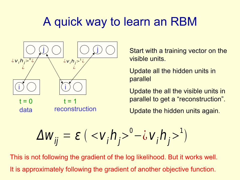
A quick way to learn an RBM

¿v ih j0¿

¿

¿v ih j1¿

¿

i

j

i

j

t = 0 t = 1

Δw ij = ε v ih j0−¿v ih j

1

Start with a training vector on the visible units.

Update all the hidden units in parallel

Update the all the visible units in parallel to get a “reconstruction”.

Update the hidden units again.

This is not following the gradient of the log likelihood. But it works well.

It is approximately following the gradient of another objective function.

reconstructiondata

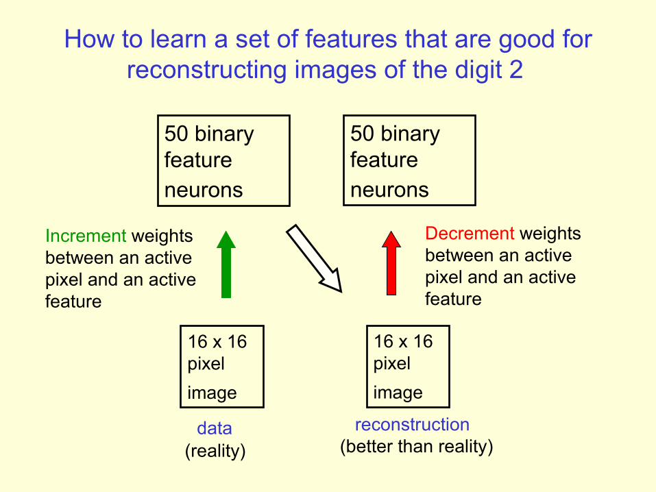
How to learn a set of features that are good for reconstructing images of the digit 2

50 binary feature neurons

16 x 16 pixel

image

50 binary feature neurons

16 x 16 pixel

image

Increment weights between an active pixel and an active feature

Decrement weights between an active pixel and an active feature

data (reality)

reconstruction (better than reality)

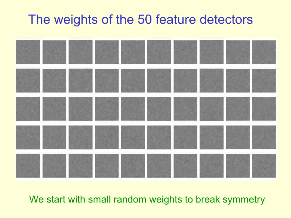
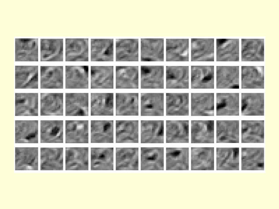
The weights of the 50 feature detectors

We start with small random weights to break symmetry

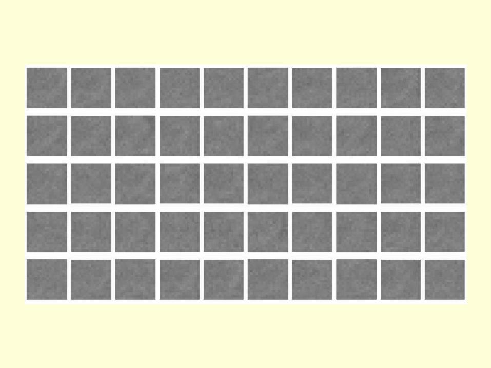
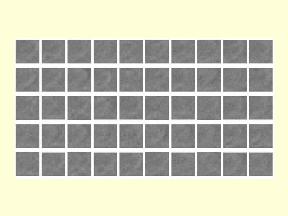
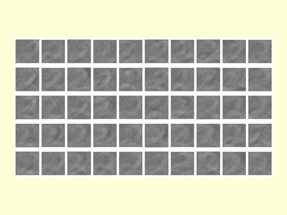
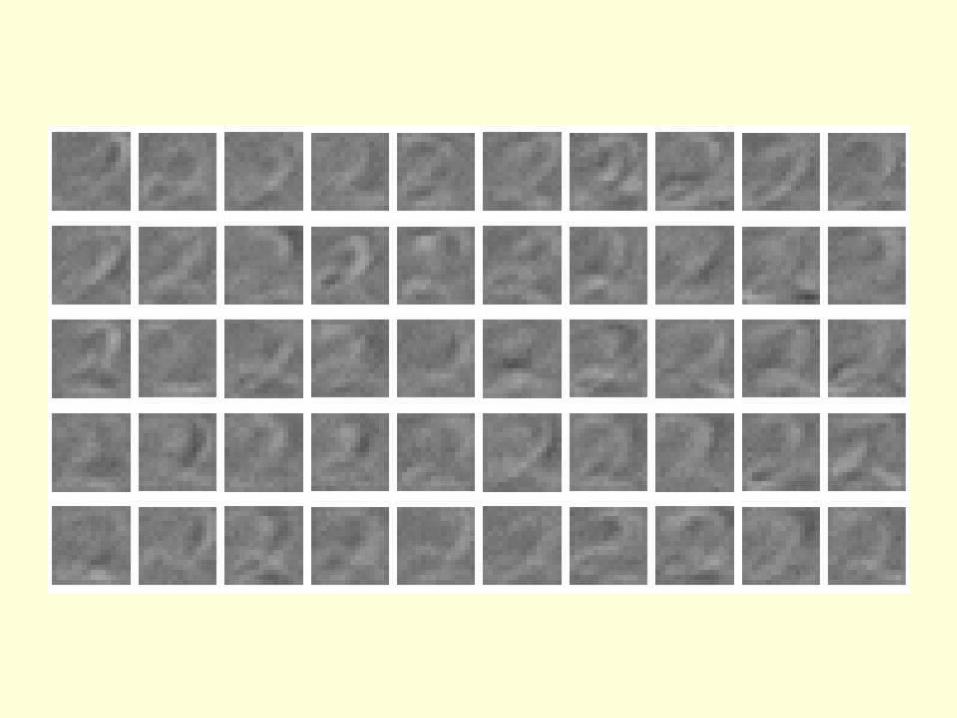
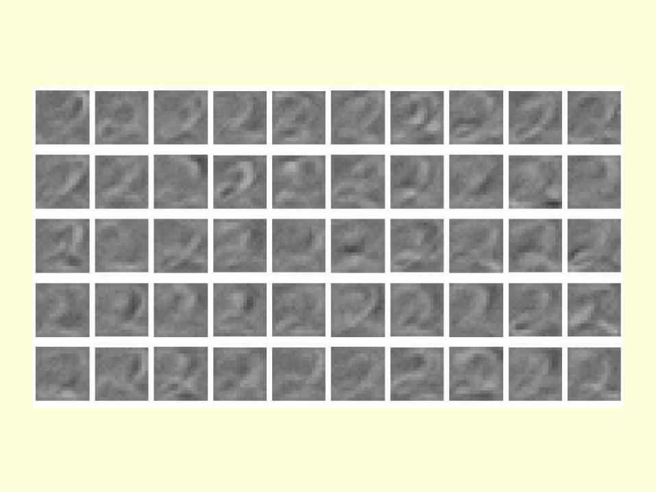
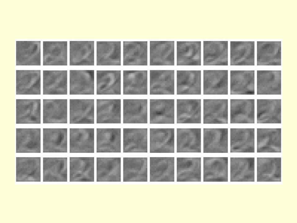
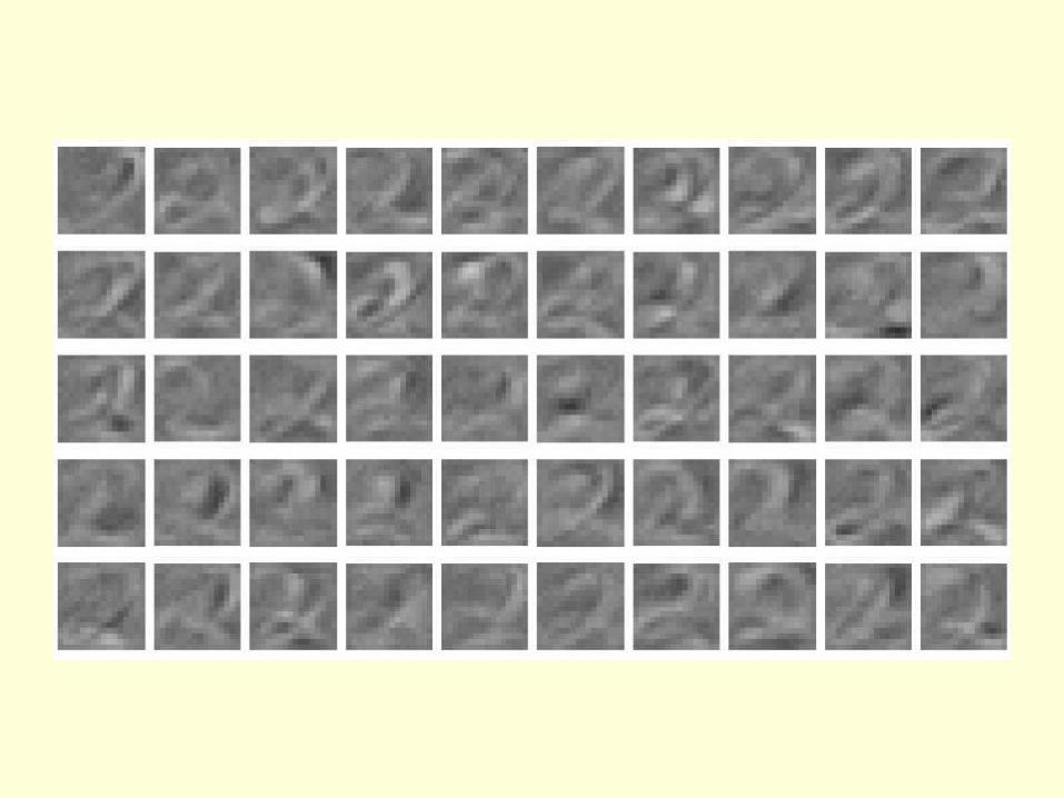
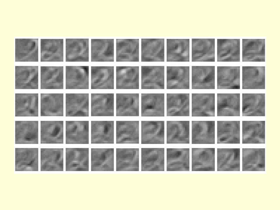
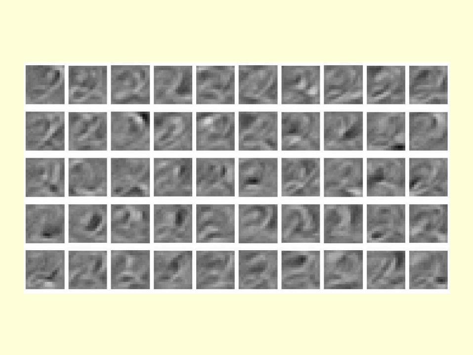
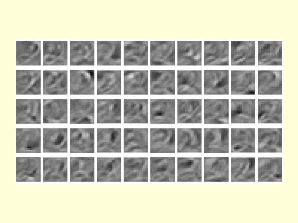
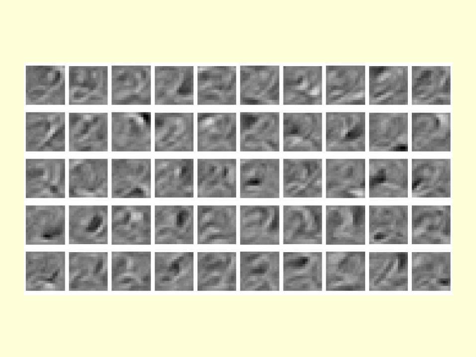
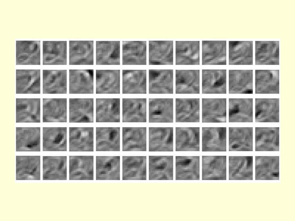
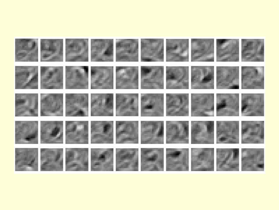
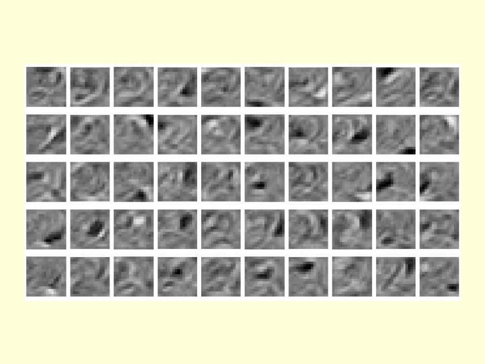
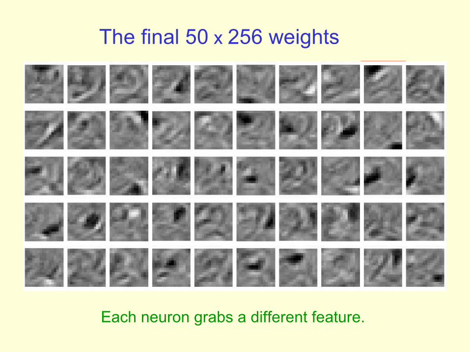
The final 50 x 256 weights

Each neuron grabs a different feature.

Reconstruction from activated binary featuresData

Reconstruction from activated binary featuresData

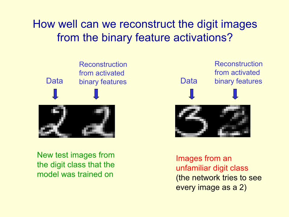
How well can we reconstruct the digit images from the binary feature activations?

New test images from the digit class that the model was trained on

Images from an unfamiliar digit class (the network tries to see every image as a 2)

Training a deep network

• First train a layer of features that receive input directly from the pixels.

• Then treat the activations of the trained features as if they were pixels and learn features of features in a second hidden layer.

• It can be proved that each time we add another layer of features we get a better model of the set of training images.– The proof is complicated. It uses variational free

energy, a method that physicists use for analyzing non-equilibrium systems.

– But it is based on a neat equivalence (described later)

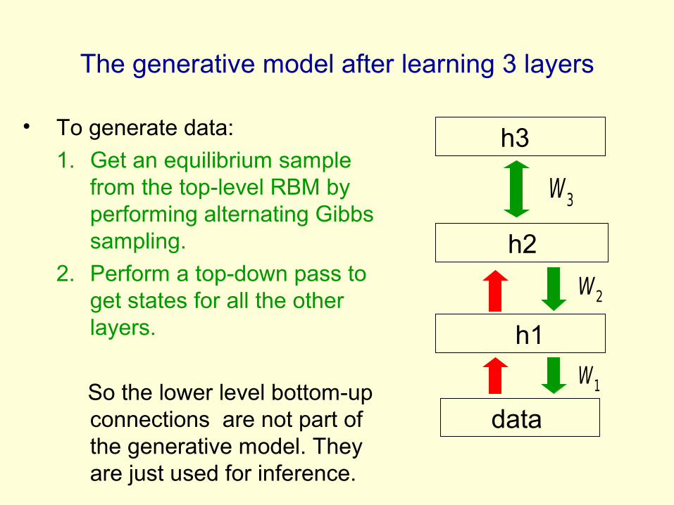
The generative model after learning 3 layers

• To generate data:

1. Get an equilibrium sample from the top-level RBM by performing alternating Gibbs sampling.

2. Perform a top-down pass to get states for all the other layers.

So the lower level bottom-up connections are not part of the generative model. They are just used for inference.

h2

data

h1

h3

W2

W3

W1

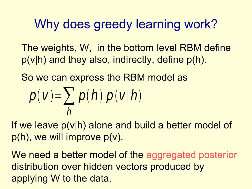
Why does greedy learning work?

pv =∑h

ph p v∣h

The weights, W, in the bottom level RBM define p(v|h) and they also, indirectly, define p(h).

So we can express the RBM model as

If we leave p(v|h) alone and build a better model of p(h), we will improve p(v).

We need a better model of the aggregated posterior distribution over hidden vectors produced by applying W to the data.

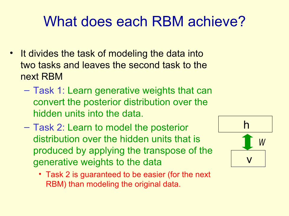
What does each RBM achieve?

• It divides the task of modeling the data into two tasks and leaves the second task to the next RBM– Task 1: Learn generative weights that can

convert the posterior distribution over the hidden units into the data.

– Task 2: Learn to model the posterior distribution over the hidden units that is produced by applying the transpose of the generative weights to the data

• Task 2 is guaranteed to be easier (for the next RBM) than modeling the original data.

h

v

W

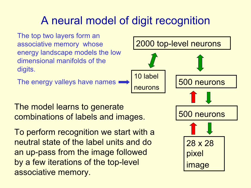
A neural model of digit recognition

2000 top-level neurons

500 neurons

500 neurons

28 x 28 pixel image

10 label

neurons

The model learns to generate combinations of labels and images.

To perform recognition we start with a neutral state of the label units and do an up-pass from the image followed by a few iterations of the top-level associative memory.

The top two layers form an associative memory whose energy landscape models the low dimensional manifolds of the digits.

The energy valleys have names

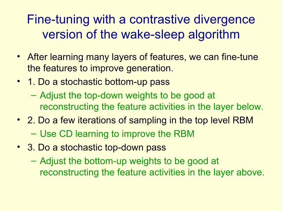
Fine-tuning with a contrastive divergence version of the wake-sleep algorithm

• After learning many layers of features, we can fine-tune the features to improve generation.

• 1. Do a stochastic bottom-up pass– Adjust the top-down weights to be good at

reconstructing the feature activities in the layer below.• 2. Do a few iterations of sampling in the top level RBM

– Use CD learning to improve the RBM

• 3. Do a stochastic top-down pass

– Adjust the bottom-up weights to be good at reconstructing the feature activities in the layer above.

Show the movie of the network generating digits

(available at www.cs.toronto/~hinton)

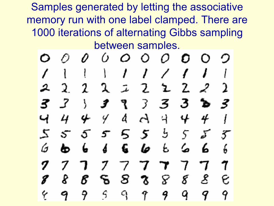
Samples generated by letting the associative memory run with one label clamped. There are 1000 iterations of alternating Gibbs sampling

between samples.

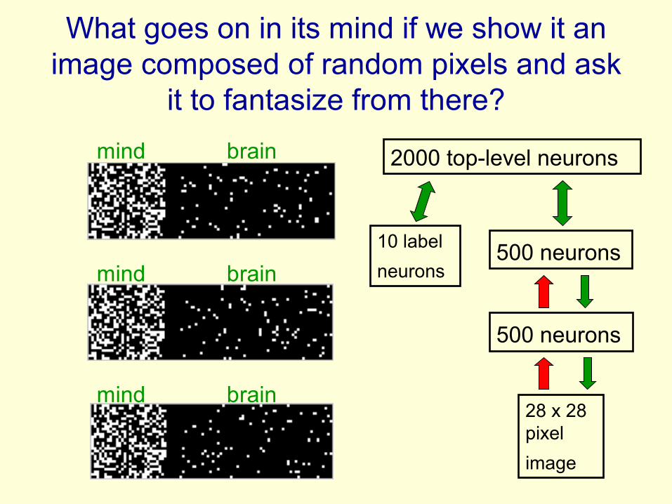
What goes on in its mind if we show it an image composed of random pixels and ask

it to fantasize from there?

mind brain

mind brain

mind brain

2000 top-level neurons

500 neurons

500 neurons

28 x 28 pixel

image

10 label

neurons

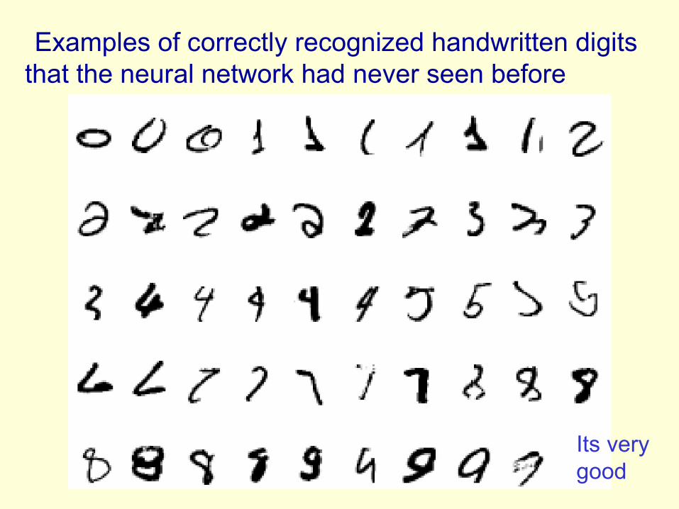
Examples of correctly recognized handwritten digitsthat the neural network had never seen before

Its very good

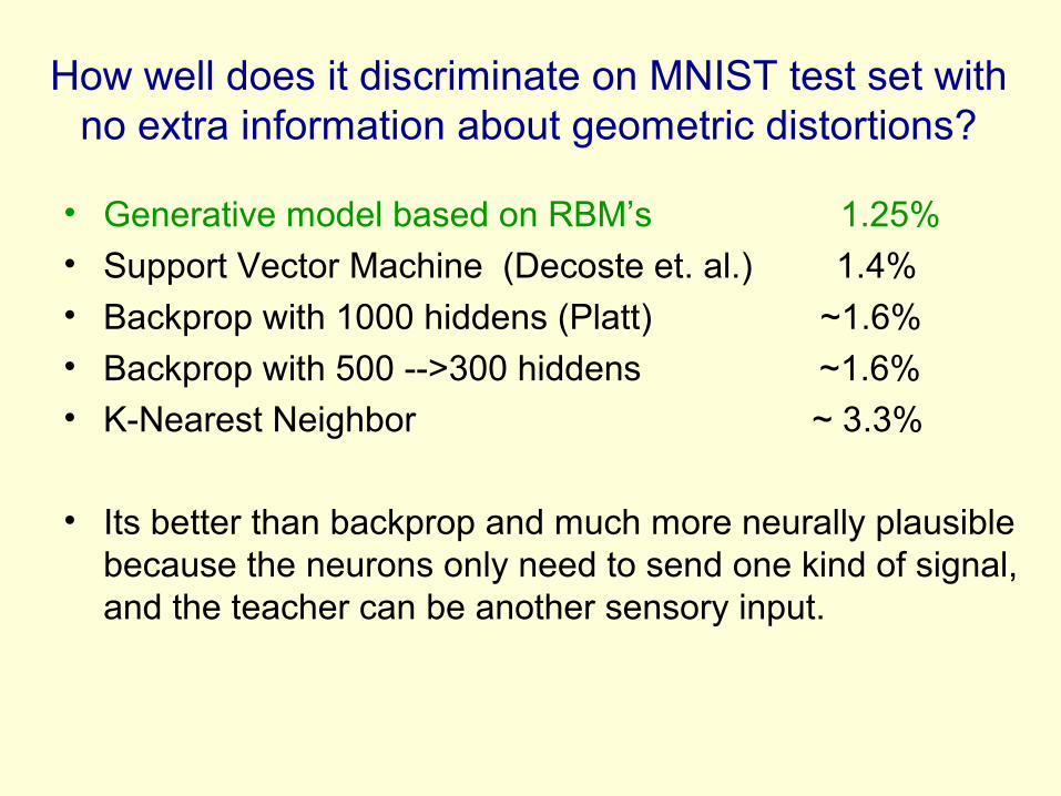
How well does it discriminate on MNIST test set with no extra information about geometric distortions?

• Generative model based on RBM’s 1.25%• Support Vector Machine (Decoste et. al.) 1.4% • Backprop with 1000 hiddens (Platt) ~1.6%• Backprop with 500 -->300 hiddens ~1.6%• K-Nearest Neighbor ~ 3.3%

• Its better than backprop and much more neurally plausible because the neurons only need to send one kind of signal, and the teacher can be another sensory input.

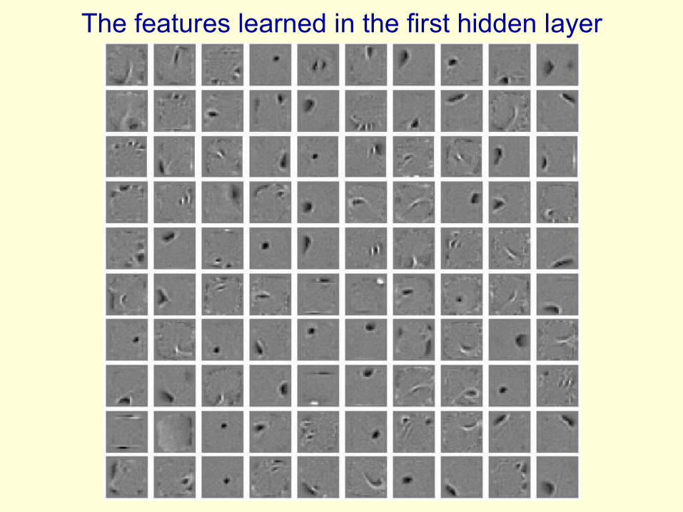
The features learned in the first hidden layer

Show the faces demo (available at www.cs.toronto/~hinton)

Another view of why layer-by-layer learning works

• There is an unexpected equivalence between RBM’s and directed networks with many layers that all use the same weights.– This equivalence also gives insight into why

contrastive divergence learning works.

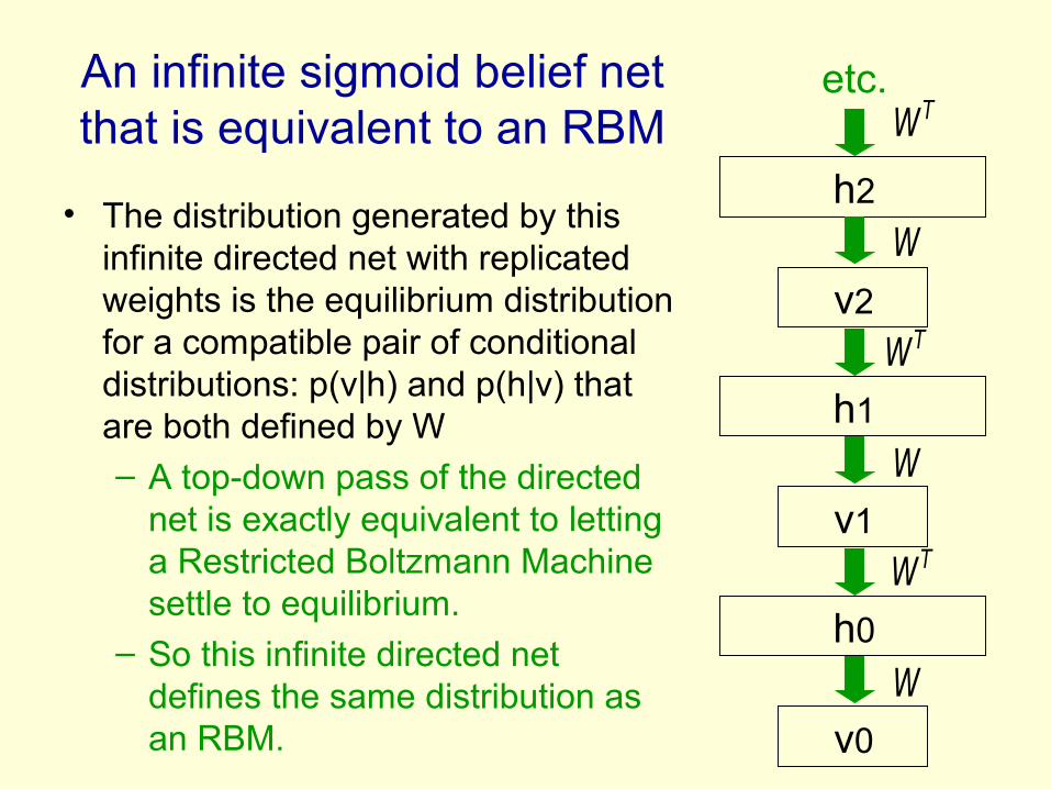
An infinite sigmoid belief net that is equivalent to an RBM

• The distribution generated by this infinite directed net with replicated weights is the equilibrium distribution for a compatible pair of conditional distributions: p(v|h) and p(h|v) that are both defined by W– A top-down pass of the directed

net is exactly equivalent to letting a Restricted Boltzmann Machine settle to equilibrium.

– So this infinite directed net defines the same distribution as an RBM.

W v1

h1

v0

h0

v2

h2

WT

WT

WT

W

W

etc.

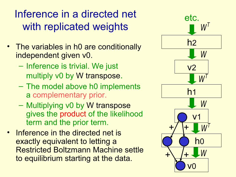
• The variables in h0 are conditionally independent given v0.– Inference is trivial. We just

multiply v0 by W transpose.– The model above h0 implements

a complementary prior.– Multiplying v0 by W transpose

gives the product of the likelihood term and the prior term.

• Inference in the directed net is exactly equivalent to letting a Restricted Boltzmann Machine settle to equilibrium starting at the data.

Inference in a directed net with replicated weights

W v1

h1

v0

h0

v2

h2

WT

WT

WT

W

W

etc.

+

+

+

+

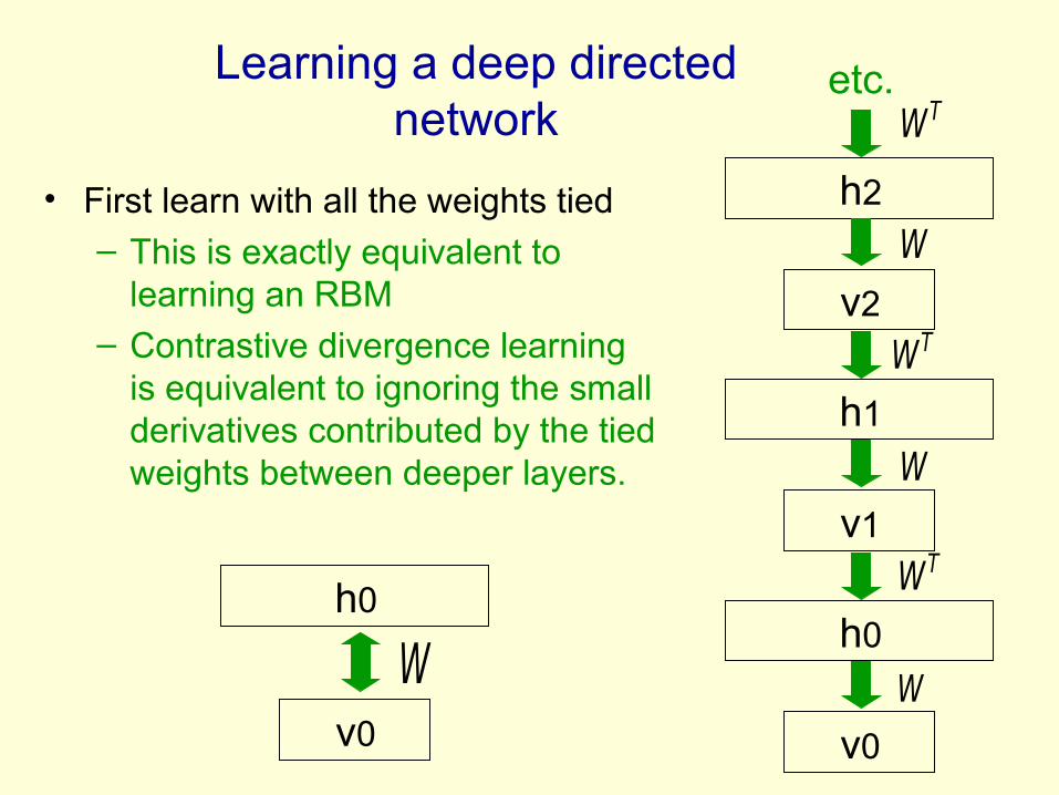
• First learn with all the weights tied– This is exactly equivalent to

learning an RBM– Contrastive divergence learning

is equivalent to ignoring the small derivatives contributed by the tied weights between deeper layers.

Learning a deep directed network

W

W v1

h1

v0

h0

v2

h2

WT

WT

WT

W

etc.

v0

h0

W

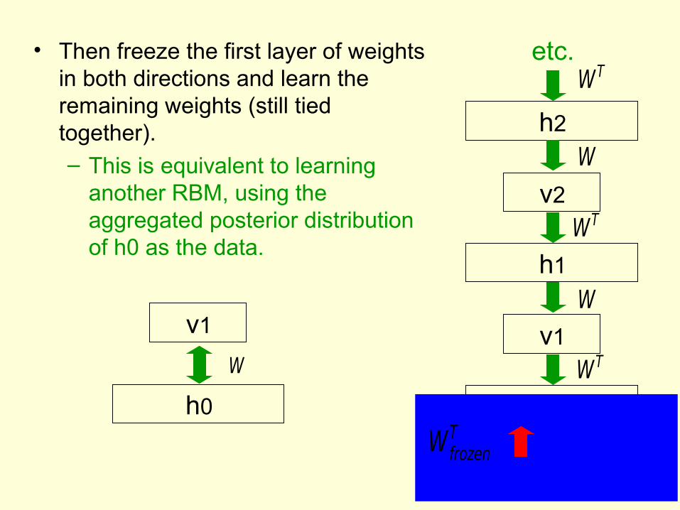
• Then freeze the first layer of weights in both directions and learn the remaining weights (still tied together).– This is equivalent to learning

another RBM, using the aggregated posterior distribution of h0 as the data.

W v1

h1

v0

h0

v2

h2

WT

WT

WT

W

etc.

W frozen

v1

h0

W

W frozenT

What happens when the weights in higher layers become different from the weights in the first layer?

• The higher layers no longer implement a complementary prior.– So performing inference using the frozen weights in

the first layer is no longer correct. – Using this incorrect inference procedure gives a

variational lower bound on the log probability of the data.

• We lose by the slackness of the bound.

• The higher layers learn a prior that is closer to the aggregated posterior distribution of the first hidden layer.– This improves the network’s model of the data.

• Hinton, Osindero and Teh (2006) prove that this improvement is always bigger than the loss.

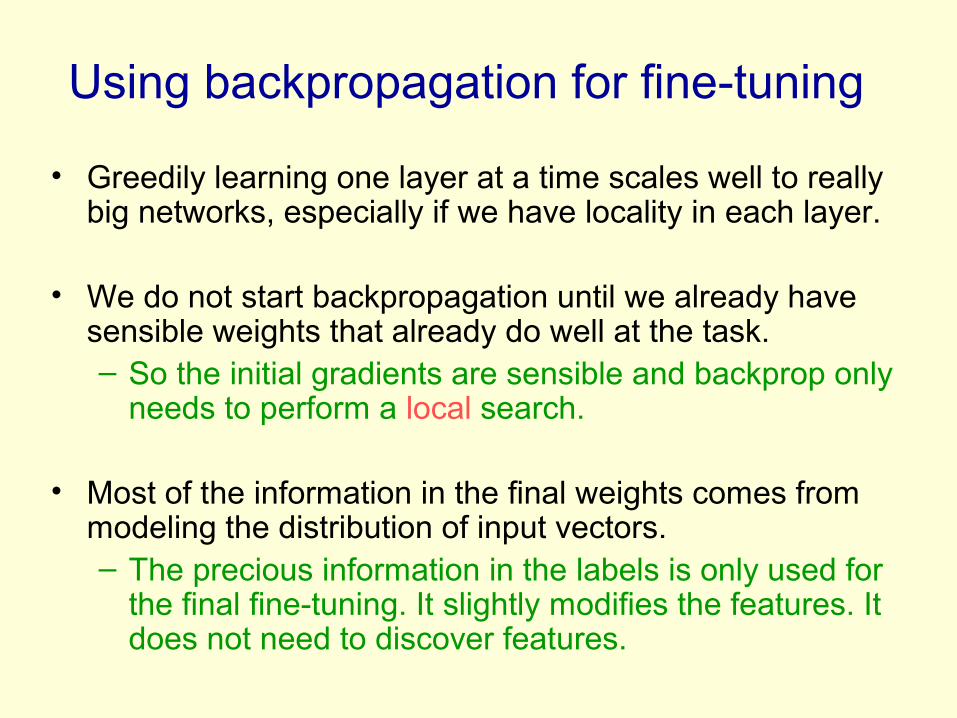
Using backpropagation for fine-tuning

• Greedily learning one layer at a time scales well to really big networks, especially if we have locality in each layer.

• We do not start backpropagation until we already have sensible weights that already do well at the task.– So the initial gradients are sensible and backprop only

needs to perform a local search.

• Most of the information in the final weights comes from modeling the distribution of input vectors. – The precious information in the labels is only used for

the final fine-tuning. It slightly modifies the features. It does not need to discover features.

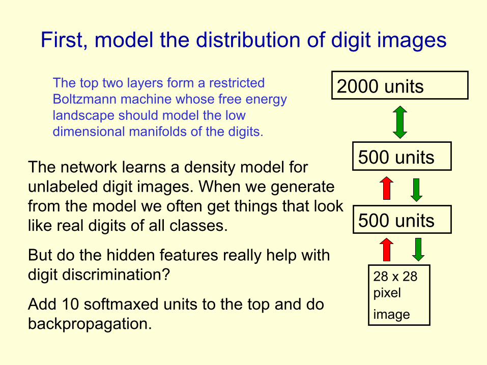
First, model the distribution of digit images

2000 units

500 units

500 units

28 x 28 pixel

image

The network learns a density model for unlabeled digit images. When we generate from the model we often get things that look like real digits of all classes.

But do the hidden features really help with digit discrimination?

Add 10 softmaxed units to the top and do backpropagation.

The top two layers form a restricted Boltzmann machine whose free energy landscape should model the low dimensional manifolds of the digits.

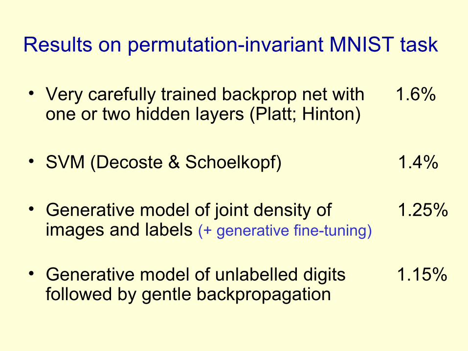
Results on permutation-invariant MNIST task

• Very carefully trained backprop net with 1.6% one or two hidden layers (Platt; Hinton)

• SVM (Decoste & Schoelkopf) 1.4%

• Generative model of joint density of 1.25% images and labels (+ generative fine-tuning)

• Generative model of unlabelled digits 1.15% followed by gentle backpropagation

Time series models

• Inference is difficult in directed models of time series if they are non-linear and they use distributed representations.

• So people tend to avoid distributed representations and use exponentially weaker methods (HMM’s) that are based on the idea that each visible frame of data has a single hidden cause

– During generation from an HMM, each frame comes from one hidden state of the HMM

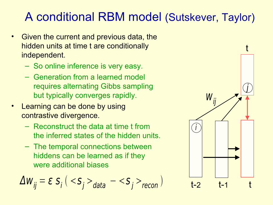
A conditional RBM model (Sutskever, Taylor)

• Given the current and previous data, the hidden units at time t are conditionally independent.

– So online inference is very easy.

– Generation from a learned model requires alternating Gibbs sampling but typically converges rapidly.

• Learning can be done by using contrastive divergence.

– Reconstruct the data at time t from the inferred states of the hidden units.

– The temporal connections between hiddens can be learned as if they were additional biases

t-2 t-1 t

t

Δw ij = ε si s j data −s j recon

j

i

w ij

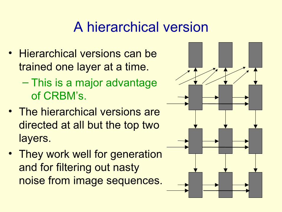
A hierarchical version

• Hierarchical versions can be trained one layer at a time.– This is a major advantage

of CRBM’s.• The hierarchical versions are

directed at all but the top two layers.

• They work well for generation and for filtering out nasty noise from image sequences.

An application to modeling motion capture data

• Human motion can be captured by placing reflective markers on the joints and then using lots of infrared cameras to track the 3-D positions of the markers.

• The 3-D positions of the markers can be converted into a frame of data containing:

– all the joint angles– 3 variables for the translation of the pelvis– 3 variables for the orientation of the pelvis

Modeling multiple types of motion

• We can easily learn to model walking and running in a single model.

• This means we can share a lot of knowledge.

• It also makes it much easier to learn nice transitions between walking and running.

Show Graham Taylor’s movies

(available via www.cs.toronto/~hinton)

Summary so far

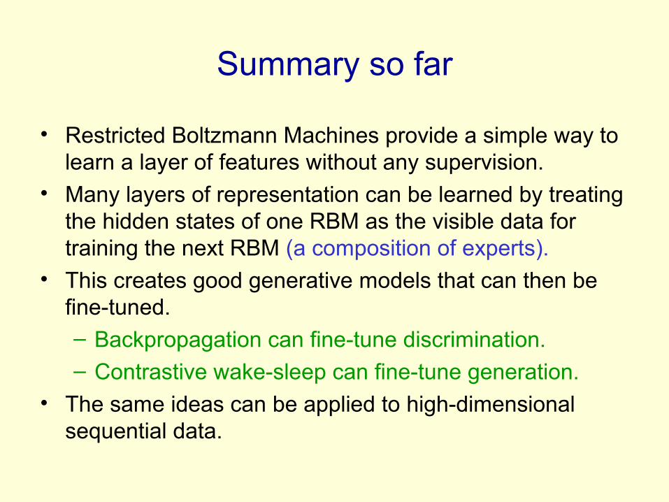
• Restricted Boltzmann Machines provide a simple way to learn a layer of features without any supervision.

• Many layers of representation can be learned by treating the hidden states of one RBM as the visible data for training the next RBM (a composition of experts).

• This creates good generative models that can then be fine-tuned.– Backpropagation can fine-tune discrimination. – Contrastive wake-sleep can fine-tune generation.

• The same ideas can be applied to high-dimensional sequential data.

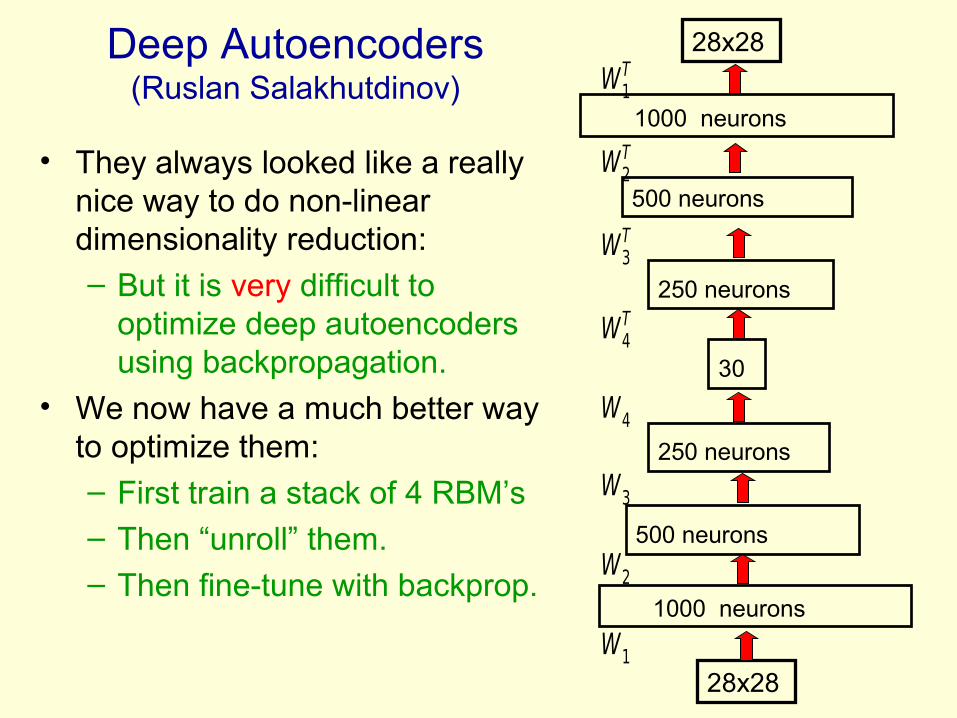
Deep Autoencoders(Ruslan Salakhutdinov)

• They always looked like a really nice way to do non-linear dimensionality reduction:– But it is very difficult to

optimize deep autoencoders using backpropagation.

• We now have a much better way to optimize them:– First train a stack of 4 RBM’s– Then “unroll” them.

– Then fine-tune with backprop.

1000 neurons

500 neurons

500 neurons

250 neurons

250 neurons

30

1000 neurons

28x28

28x28

W1T

W2T

W3T

W4T

W4

W3

W2

W1

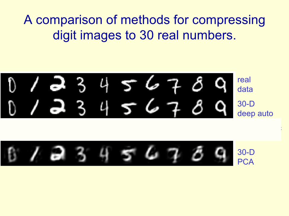
A comparison of methods for compressing digit images to 30 real numbers.

real data

30-D deep auto

30-D logistic PCA

30-D PCA

Do the 30-D codes found by the autoencoder preserve the class

structure of the data?

• Take the 30-D activity patterns in the code layer and display them in 2-D using a new form of non-linear multi-dimensional scaling (UNI-SNE)

• Will the learning find the natural classes?

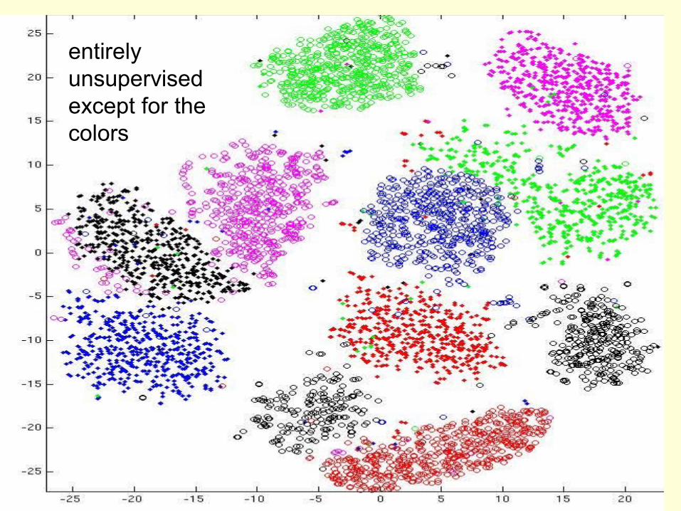
entirely unsupervised except for the colors

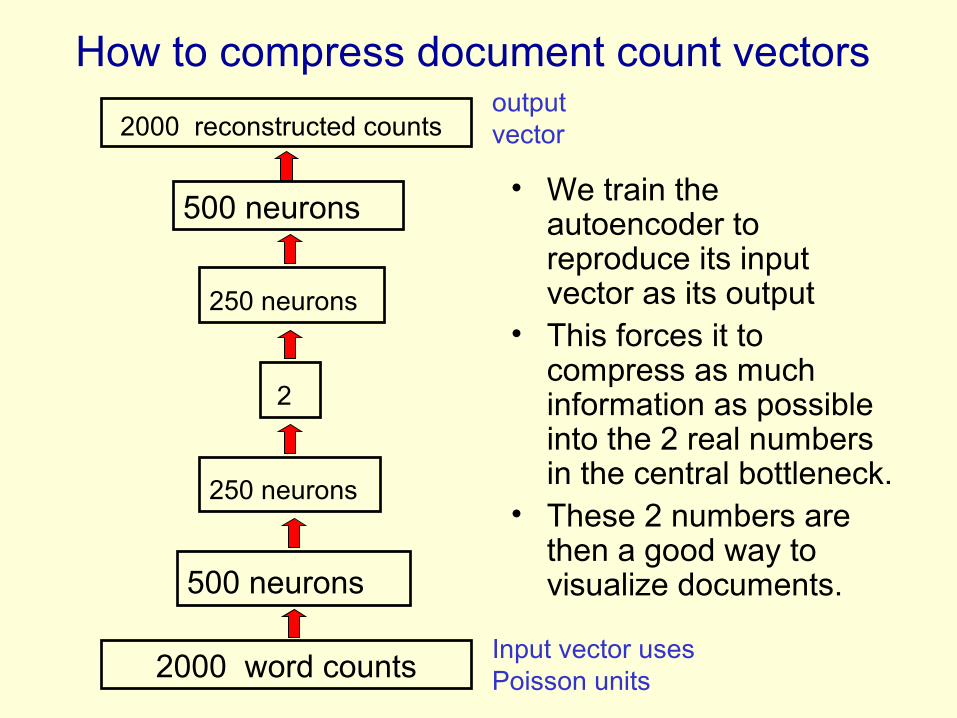
How to compress document count vectors

• We train the autoencoder to reproduce its input vector as its output

• This forces it to compress as much information as possible into the 2 real numbers in the central bottleneck.

• These 2 numbers are then a good way to visualize documents.

2000 reconstructed counts

500 neurons

2000 word counts

500 neurons

250 neurons

250 neurons

2

Input vector uses Poisson units

output vector

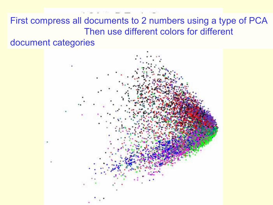
First compress all documents to 2 numbers using a type of PCA Then use different colors for different document categories

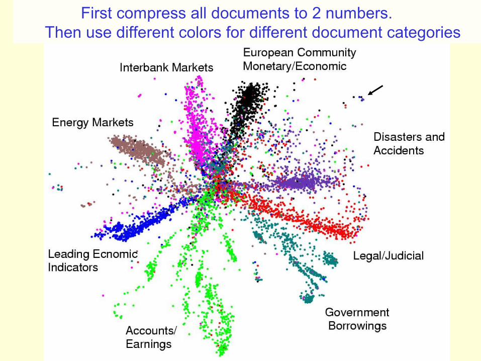
First compress all documents to 2 numbers. Then use different colors for different document categories

The fastest possible way to find similar documents

• Given a query document, how long does it take to find a shortlist of 10,000 similar documents in a set of one billion documents?– Would you be happy with one millesecond?

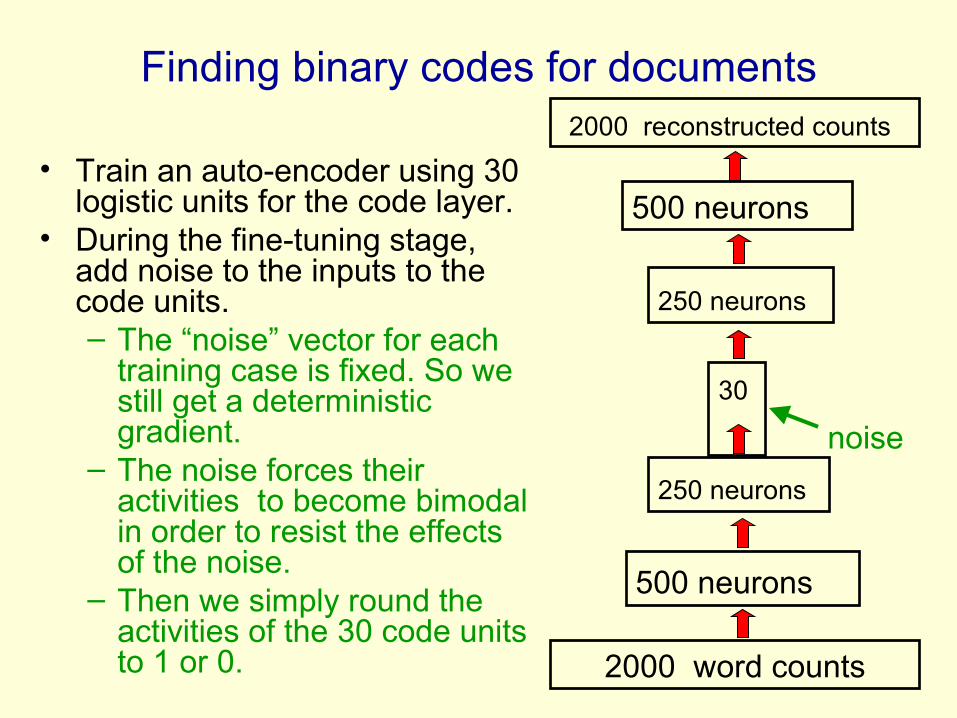
Finding binary codes for documents

• Train an auto-encoder using 30 logistic units for the code layer.

• During the fine-tuning stage, add noise to the inputs to the code units.– The “noise” vector for each

training case is fixed. So we still get a deterministic gradient.

– The noise forces their activities to become bimodal in order to resist the effects of the noise.

– Then we simply round the activities of the 30 code units to 1 or 0.

2000 reconstructed counts

500 neurons

2000 word counts

500 neurons

250 neurons

250 neurons

30 noise

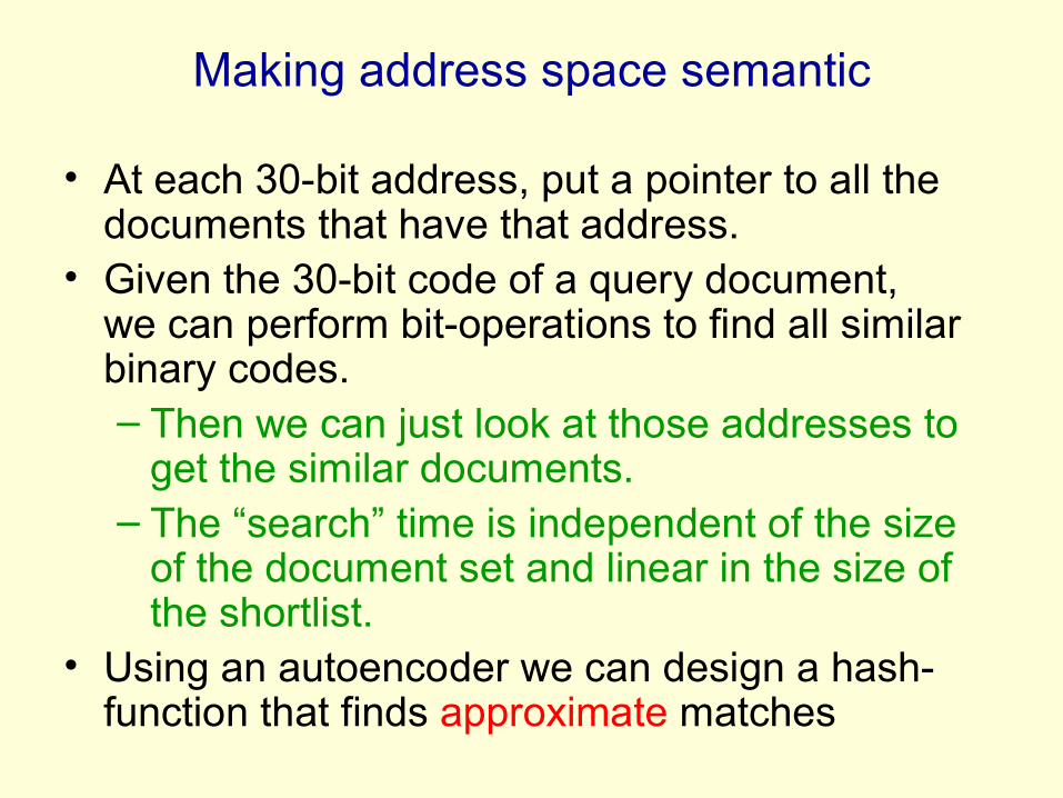
Making address space semantic

• At each 30-bit address, put a pointer to all the documents that have that address.

• Given the 30-bit code of a query document, we can perform bit-operations to find all similar binary codes.– Then we can just look at those addresses to

get the similar documents.– The “search” time is independent of the size

of the document set and linear in the size of the shortlist.

• Using an autoencoder we can design a hash-function that finds approximate matches

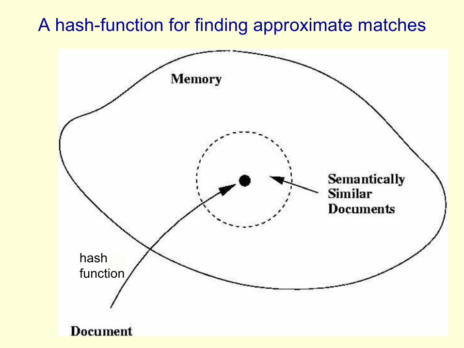
A hash-function for finding approximate matches

hash function

How good is a shortlist found this way?

• We have only implemented it for a million documents with 20-bit codes --- but what could possibly go wrong?– A 20-D hypercube allows us to capture enough

of the similarity structure of our document set. • The shortlist found using binary codes actually

improves the precision-recall curves of TF-IDF.– Locality sensitive hashing (the fastest other

method) is 50 times slower and always performs worse than TF-IDF alone.

THE END

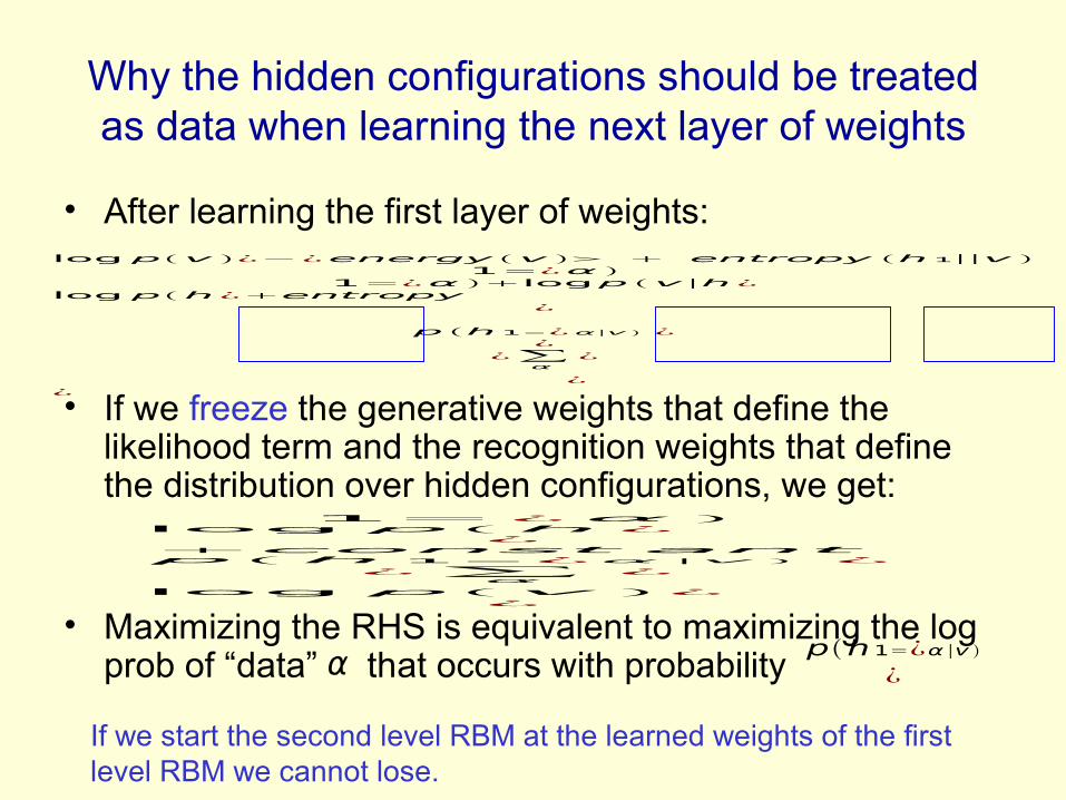
• After learning the first layer of weights:

• If we freeze the generative weights that define the likelihood term and the recognition weights that define the distribution over hidden configurations, we get:

• Maximizing the RHS is equivalent to maximizing the log prob of “data” that occurs with probability

Why the hidden configurations should be treated as data when learning the next layer of weights

logpv ¿−¿energy v entropy h1∣∣v 1=¿α

1=¿α logp v∣h¿logph¿entropy

¿

p h1=¿α∣v ¿¿

¿∑α

¿

¿

¿

1=¿α

logph¿¿

const antph1=¿α∣v ¿

¿∑α

¿

logpv ¿¿

ph1=¿α∣v

¿α

If we start the second level RBM at the learned weights of the first level RBM we cannot lose.

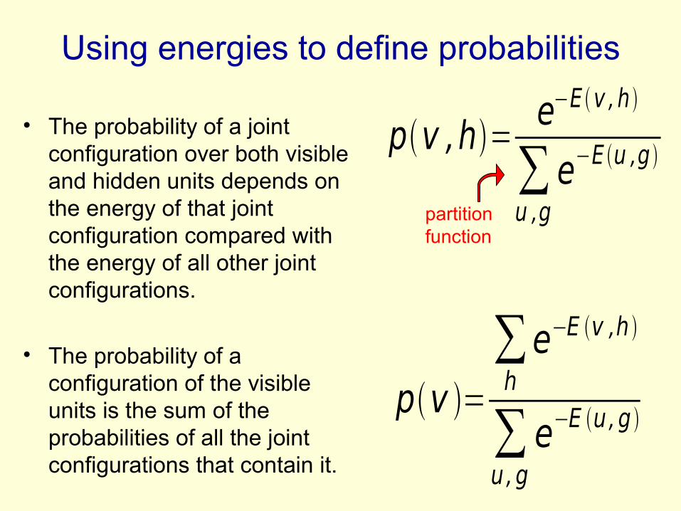
Using energies to define probabilities

• The probability of a joint configuration over both visible and hidden units depends on the energy of that joint configuration compared with the energy of all other joint configurations.

• The probability of a configuration of the visible units is the sum of the probabilities of all the joint configurations that contain it.

pv ,h=e−E v ,h

∑u ,g

e−E u ,g

pv =∑he−E v ,h

∑u,g

e−E u,g

partition function

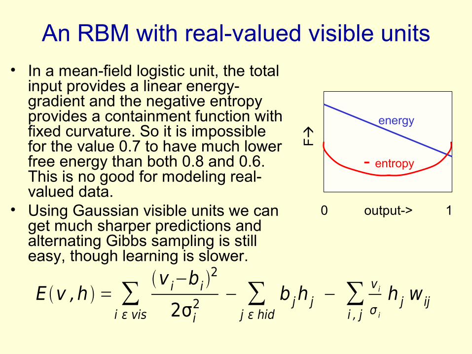
An RBM with real-valued visible units

• In a mean-field logistic unit, the total input provides a linear energy-gradient and the negative entropy provides a containment function with fixed curvature. So it is impossible for the value 0.7 to have much lower free energy than both 0.8 and 0.6. This is no good for modeling real-valued data.

• Using Gaussian visible units we can get much sharper predictions and alternating Gibbs sampling is still easy, though learning is slower.

E v ,h = ∑i ε vis

v i−b i 2

2σi2

− ∑j ε hid

b jh j − ∑i , j

v i

σ i

h j w ij

0 output-> 1

F

energy

- entropy

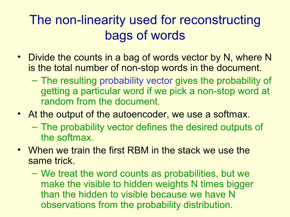
The non-linearity used for reconstructing bags of words

• Divide the counts in a bag of words vector by N, where N is the total number of non-stop words in the document.– The resulting probability vector gives the probability of

getting a particular word if we pick a non-stop word at random from the document.

• At the output of the autoencoder, we use a softmax.– The probability vector defines the desired outputs of

the softmax. • When we train the first RBM in the stack we use the

same trick. – We treat the word counts as probabilities, but we

make the visible to hidden weights N times bigger than the hidden to visible because we have N observations from the probability distribution.

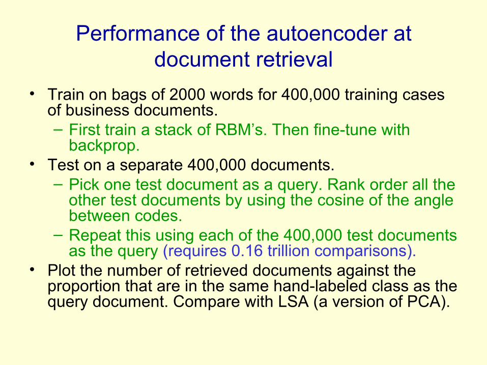
Performance of the autoencoder at document retrieval

• Train on bags of 2000 words for 400,000 training cases of business documents.– First train a stack of RBM’s. Then fine-tune with

backprop.• Test on a separate 400,000 documents.

– Pick one test document as a query. Rank order all the other test documents by using the cosine of the angle between codes.

– Repeat this using each of the 400,000 test documents as the query (requires 0.16 trillion comparisons).

• Plot the number of retrieved documents against the proportion that are in the same hand-labeled class as the query document. Compare with LSA (a version of PCA).

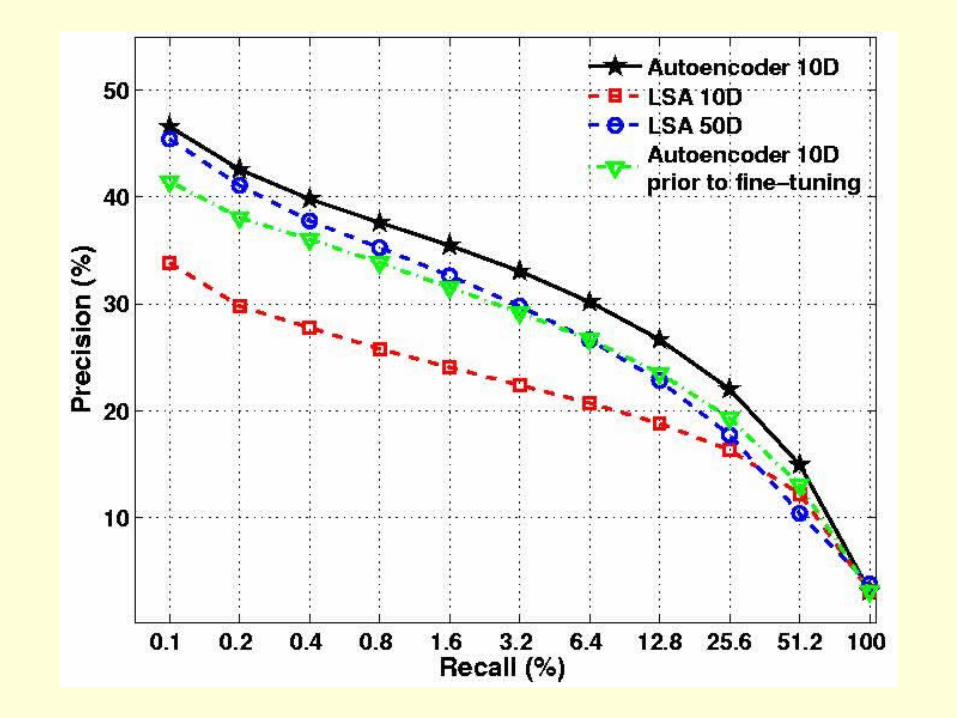
Proportion of retrieved documents in same class as query

Number of documents retrieved