An Efficient Explanation of Individual Classifications using Game Theory

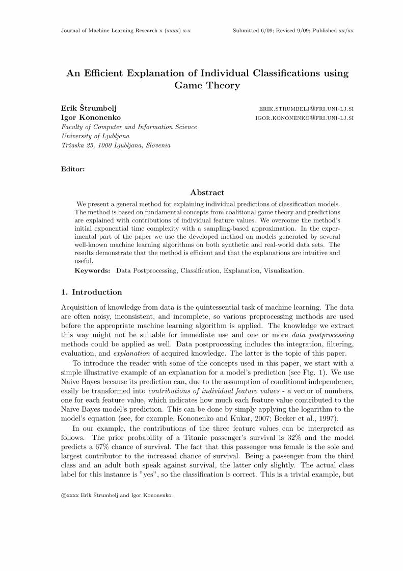
Journal of Machine Learning Research x (xxxx) x-x Submitted 6/09; Revised 9/09; Published xx/xx

An Efficient Explanation of Individual Classifications usingGame Theory

Erik Strumbelj [email protected]

Igor Kononenko [email protected]

Faculty of Computer and Information ScienceUniversity of LjubljanaTrzaska 25, 1000 Ljubljana, Slovenia

Editor:

Abstract

We present a general method for explaining individual predictions of classification models.The method is based on fundamental concepts from coalitional game theory and predictionsare explained with contributions of individual feature values. We overcome the method’sinitial exponential time complexity with a sampling-based approximation. In the exper-imental part of the paper we use the developed method on models generated by severalwell-known machine learning algorithms on both synthetic and real-world data sets. Theresults demonstrate that the method is efficient and that the explanations are intuitive anduseful.Keywords: Data Postprocessing, Classification, Explanation, Visualization.

1. Introduction

Acquisition of knowledge from data is the quintessential task of machine learning. The dataare often noisy, inconsistent, and incomplete, so various preprocessing methods are usedbefore the appropriate machine learning algorithm is applied. The knowledge we extractthis way might not be suitable for immediate use and one or more data postprocessingmethods could be applied as well. Data postprocessing includes the integration, filtering,evaluation, and explanation of acquired knowledge. The latter is the topic of this paper.

To introduce the reader with some of the concepts used in this paper, we start with asimple illustrative example of an explanation for a model’s prediction (see Fig. 1). We useNaive Bayes because its prediction can, due to the assumption of conditional independence,easily be transformed into contributions of individual feature values - a vector of numbers,one for each feature value, which indicates how much each feature value contributed to theNaive Bayes model’s prediction. This can be done by simply applying the logarithm to themodel’s equation (see, for example, Kononenko and Kukar, 2007; Becker et al., 1997).

In our example, the contributions of the three feature values can be interpreted asfollows. The prior probability of a Titanic passenger’s survival is 32% and the modelpredicts a 67% chance of survival. The fact that this passenger was female is the sole andlargest contributor to the increased chance of survival. Being a passenger from the thirdclass and an adult both speak against survival, the latter only slightly. The actual classlabel for this instance is ”yes”, so the classification is correct. This is a trivial example, but

c©xxxx Erik Strumbelj and Igor Kononenko.

Strumbelj and Kononenko

providing the end-user with such an explanation on top of a prediction, makes the predictioneasier to understand and to trust. The latter is crucial in situations where important andsensitive decisions are made. One such example is medicine, where medical practitionersare known to be reluctant to use machine learning models, despite their often superiorperformance (Kononenko, 2001). The inherent ability of explaining its decisions is one ofthe main reasons for the frequent use of the Naive Bayes classifier in medical diagnosisand prognosis (Kononenko, 2001). The approach used to explain the decision in Fig. 1 isspecific to Naive Bayes, but can we design an explanation method which works for any typeof classifier? In this paper we address this question and propose a method for explainingthe predictions of classification models, which can be applied to any classifier in a uniformway.

Figure 1: An instance from the well-known Titanic data set with the Naive Bayesmodel’s prediction and an explanation in the form of contributions of in-dividual feature values. A copy of the Titanic dataset can be found athttp://www.ailab.si/orange/datasets.psp.

1.1 Related Work

Before addressing general explanation methods, we list a few model-specific methods toemphasize two things. First, most models have model-specific explanation methods. Andsecond, providing an explanation in the form of contributions of feature values is a commonapproach. Note that many more model-specific explanation methods exist and this is farfrom being a complete reference. Similar to Naive Bayes, other machine learning modelsalso have an inherent explanation. For example, a decision tree’s prediction is made byfollowing a decision rule from the root to the leaf, which contains the instance. Decisionrules and Bayesian networks are also examples of transparent classifiers. Nomograms are away of visualizing contributions of feature values and were applied to Naive Bayes (Mozinaet al., 2004) and, in a limited way (linear kernel functions), to SVM (Jakulin et al., 2005).Other related work focusses on explaining the SVM model, most recently in the form ofvisualization (Poulet, 2004; Hamel, 2006) and rule-extraction (Martens et al., 2007). TheExplainD framework (Szafron et al., 2006) provides explanations for additive classifiers inthe form of contributions. Breiman provided additional tools for showing how individualfeatures contribute to the predictions of his Random Forests (Breiman, 2001). The ex-planation and interpretation of artificial neural networks, which are arguably one of the

2

Explaining Individual Classifications

least transparent models, has also received a lot of attention, especially in the form of ruleextraction (Towell and Shavlik, 1993; Andrews et al., 1995; Nayak, 2009).

So, why do we even need a general explanation method? It is not difficult to think ofa reasonable scenario where a general explanation method would be useful. For example,imagine a user using a classifier and a corresponding explanation method. At some point themodel might be replaced with a better performing model of a different type, which usuallymeans that the explanation method also has to be modified or replaced. The user then hasto invest time and effort into adapting to the new explanation method. This can be avoidedby using a general explanation method. Overall, a good general explanation method reducesthe dependence between the user-end and the underlying machine learning methods, whichmakes work with machine learning models more user-friendly. This is especially desirable incommercial applications and applications of machine learning in fields outside of machinelearning, such as medicine, marketing, etc. An effective and efficient general explanationmethod would also be a useful tool for comparing how a model predicts different instancesand how different models predict the same instance.

As far as the authors are aware, there exist two other general explanation methods forexplaining a model’s prediction: the work by Robnik-Sikonja and Kononenko (2008) andthe work by Lemaire et al. (2008). While there are several differences between the twomethods, both explain a prediction with contributions of feature values and both use thesame basic approach. A feature value’s contribution is defined as the difference between themodel’s initial prediction and its average prediction across perturbations of the correspond-ing feature. In other words, we look at how the prediction would change if we ”ignore”the feature value. This myopic approach can lead to serious errors if the feature valuesare conditionally dependent, which is especially evident when a disjunctive concept (or anyother form of redundancy) is present. We can use a simple example to illustrate how thesemethods work. Imagine we ask someone who is knowledgeable in boolean logic What willthe result of (1 OR 1) be?. It will be one, of course. Now we mask the first value and askagain What will the result of (something OR 1) be?. It will still be one. So, it does not mat-ter if the person knows or does not know the first value - the result does not change. Hence,we conclude that the first value is irrelevant for that persons decision regarding whether theresult will be 1 or 0. Symmetrically, we can conclude that the second value is also irrelevantfor the persons decision making process. Therefore, both values are irrelevant. This is, ofcourse, an incorrect explanation of how these two values contribute to the persons decision.

Further details and examples of where existing methods would fail can be found in ourprevious work (Strumbelj et al., 2009), where we suggest observing the changes across allpossible subsets of features values. While this effectively deals with the shortcomings ofprevious methods, it suffers from an exponential time complexity.

To summarize, we have existing general explanation methods, which sacrifice a part oftheir effectiveness for efficiency, and we know that generating effective contributions requiresobserving the power set of all features, which is far from efficient. The contribution of thispaper and its improvement over our previous work is twofold. First, we provide a rigoroustheoretical analysis of our explanation method and link it with known concepts from gametheory, thus formalizing some of its desirable properties. And second, we propose an efficientsampling-based approximation method, which overcomes the exponential time complexityand does not require retraining the classifier.

3


The remainder of this paper is organized as follows. Section 2 introduces some basicconcepts from classification and coalitional game theory. In Section 3 we provide the theo-retical foundations, the approximation method, and a simple illustrative example. Section4 covers the experimental part of our work. With Section 5 we conclude the paper andprovide ideas for future work.

2. Preliminaries

First, we introduce some basic concepts from classification and coalitional game theory,which are used in the formal description of our explanation method.

2.1 Classification.

In machine learning classification is a form of supervised learning where the objective is topredict the class label for unlabelled input instances, each described by feature values froma feature space. Predictions are based on background knowledge and knowledge extracted(that is, learned) from a sample of labelled instances (usually in the form of a training set).

Definition 1 The feature space A is the cartesian product of n features (represented withthe set N = {1, 2, ..., n}): A = A1 × A2 × ... × An, where each feature Ai is a finite set offeature values.

Remark 1 With this definition of a feature space we limit ourselves to finite (that is,discrete) features. However, we later show that this restriction does not apply to the ap-proximation method, which can handle both discrete and continuous features.

To formally describe situations where feature values are ignored, we define a subspaceAS = A′1 ×A′2 × ...×A′n, where A′i = Ai if i ∈ S and A′i = {ε} otherwise. Therefore, givena set S ⊂ N , AS is a feature subspace, where features not in S are ”ignored” (AN = A).Instances from a subspace have one or more components unknown as indicated by ε. Nowwe define a classifier.

Definition 2 A classifier, f , is a mapping from a feature space to a normalized |C|-dimensional space f : A → [0, 1]|C|, where C is a finite set of labels.

Remark 2 We use a more general definition of a classifier to include classifiers whichassign a rank or score to each class label. However, in practice, we mostly deal with twospecial cases: classifiers in the traditional sense (for each vector, one of the components is1 and the rest are 0) and probabilistic classifiers (for each vector, the vector componentsalways add up to 1 and are therefore a probability distribution over the class label statespace).

2.2 Coalitional game theory.

The following concepts from coalitional game theory are used in the formalization of ourmethod, starting with the definition of a coalitional game.

4


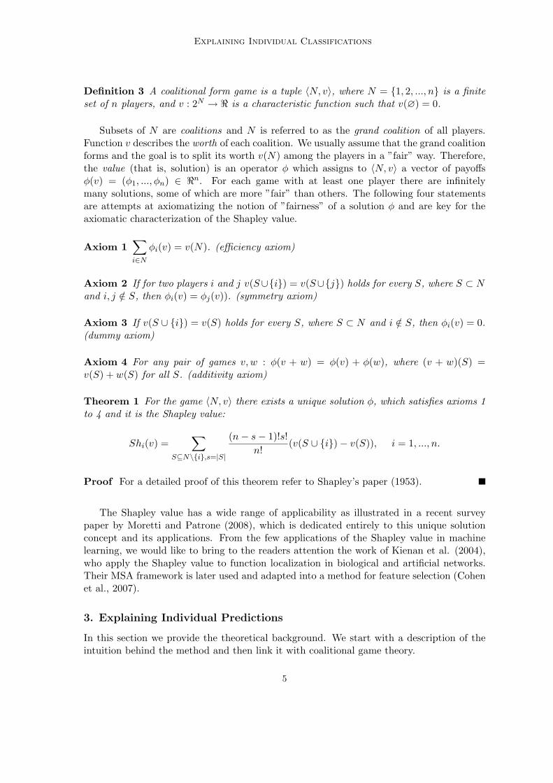
Definition 3 A coalitional form game is a tuple 〈N, v〉, where N = {1, 2, ..., n} is a finiteset of n players, and v : 2N → < is a characteristic function such that v(∅) = 0.

Subsets of N are coalitions and N is referred to as the grand coalition of all players.Function v describes the worth of each coalition. We usually assume that the grand coalitionforms and the goal is to split its worth v(N) among the players in a ”fair” way. Therefore,the value (that is, solution) is an operator φ which assigns to 〈N, v〉 a vector of payoffsφ(v) = (φ1, ..., φn) ∈ <n. For each game with at least one player there are infinitelymany solutions, some of which are more ”fair” than others. The following four statementsare attempts at axiomatizing the notion of ”fairness” of a solution φ and are key for theaxiomatic characterization of the Shapley value.

Axiom 1∑

i∈N

φi(v) = v(N). (efficiency axiom)

Axiom 2 If for two players i and j v(S∪{i}) = v(S∪{j}) holds for every S, where S ⊂ Nand i, j /∈ S, then φi(v) = φj(v)). (symmetry axiom)

Axiom 3 If v(S ∪ {i}) = v(S) holds for every S, where S ⊂ N and i /∈ S, then φi(v) = 0.(dummy axiom)

Axiom 4 For any pair of games v, w : φ(v + w) = φ(v) + φ(w), where (v + w)(S) =v(S) + w(S) for all S. (additivity axiom)

Theorem 1 For the game 〈N, v〉 there exists a unique solution φ, which satisfies axioms 1to 4 and it is the Shapley value:

Shi(v) =∑

S⊆N\{i},s=|S|

(n− s− 1)!s!n!

(v(S ∪ {i})− v(S)), i = 1, ..., n.

Proof For a detailed proof of this theorem refer to Shapley’s paper (1953).

The Shapley value has a wide range of applicability as illustrated in a recent surveypaper by Moretti and Patrone (2008), which is dedicated entirely to this unique solutionconcept and its applications. From the few applications of the Shapley value in machinelearning, we would like to bring to the readers attention the work of Kienan et al. (2004),who apply the Shapley value to function localization in biological and artificial networks.Their MSA framework is later used and adapted into a method for feature selection (Cohenet al., 2007).

3. Explaining Individual Predictions

In this section we provide the theoretical background. We start with a description of theintuition behind the method and then link it with coalitional game theory.

5


3.1 Definition of the Explanation Method

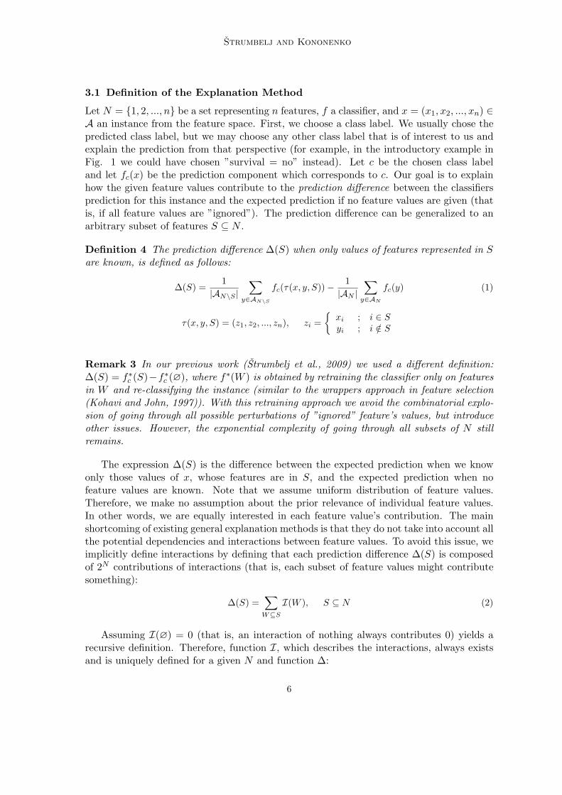
Let N = {1, 2, ..., n} be a set representing n features, f a classifier, and x = (x1, x2, ..., xn) ∈A an instance from the feature space. First, we choose a class label. We usually chose thepredicted class label, but we may choose any other class label that is of interest to us andexplain the prediction from that perspective (for example, in the introductory example inFig. 1 we could have chosen ”survival = no” instead). Let c be the chosen class labeland let fc(x) be the prediction component which corresponds to c. Our goal is to explainhow the given feature values contribute to the prediction difference between the classifiersprediction for this instance and the expected prediction if no feature values are given (thatis, if all feature values are ”ignored”). The prediction difference can be generalized to anarbitrary subset of features S ⊆ N .

Definition 4 The prediction difference ∆(S) when only values of features represented in Sare known, is defined as follows:

∆(S) =1

|AN\S |∑

y∈AN\S

fc(τ(x, y, S))− 1|AN |

∑

y∈AN

fc(y) (1)

τ(x, y, S) = (z1, z2, ..., zn), zi ={

xi ; i ∈ Syi ; i /∈ S

Remark 3 In our previous work (Strumbelj et al., 2009) we used a different definition:∆(S) = f∗c (S)−f∗c (∅), where f∗(W ) is obtained by retraining the classifier only on featuresin W and re-classifying the instance (similar to the wrappers approach in feature selection(Kohavi and John, 1997)). With this retraining approach we avoid the combinatorial explo-sion of going through all possible perturbations of ”ignored” feature’s values, but introduceother issues. However, the exponential complexity of going through all subsets of N stillremains.

The expression ∆(S) is the difference between the expected prediction when we knowonly those values of x, whose features are in S, and the expected prediction when nofeature values are known. Note that we assume uniform distribution of feature values.Therefore, we make no assumption about the prior relevance of individual feature values.In other words, we are equally interested in each feature value’s contribution. The mainshortcoming of existing general explanation methods is that they do not take into account allthe potential dependencies and interactions between feature values. To avoid this issue, weimplicitly define interactions by defining that each prediction difference ∆(S) is composedof 2N contributions of interactions (that is, each subset of feature values might contributesomething):

∆(S) =∑

W⊆S

I(W ), S ⊆ N (2)

Assuming I(∅) = 0 (that is, an interaction of nothing always contributes 0) yields arecursive definition. Therefore, function I, which describes the interactions, always existsand is uniquely defined for a given N and function ∆:

6


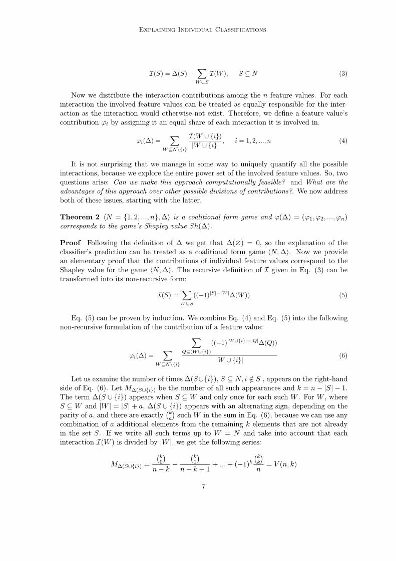
I(S) = ∆(S)−∑

W⊂S

I(W ), S ⊆ N (3)

Now we distribute the interaction contributions among the n feature values. For eachinteraction the involved feature values can be treated as equally responsible for the inter-action as the interaction would otherwise not exist. Therefore, we define a feature value’scontribution ϕi by assigning it an equal share of each interaction it is involved in.

ϕi(∆) =∑

W⊆N\{i}

I(W ∪ {i})|W ∪ {i}| , i = 1, 2, ..., n (4)

It is not surprising that we manage in some way to uniquely quantify all the possibleinteractions, because we explore the entire power set of the involved feature values. So, twoquestions arise: Can we make this approach computationally feasible? and What are theadvantages of this approach over other possible divisions of contributions?. We now addressboth of these issues, starting with the latter.

Theorem 2 〈N = {1, 2, ..., n},∆〉 is a coalitional form game and ϕ(∆) = (ϕ1, ϕ2, ..., ϕn)corresponds to the game’s Shapley value Sh(∆).

Proof Following the definition of ∆ we get that ∆(∅) = 0, so the explanation of theclassifier’s prediction can be treated as a coalitional form game 〈N, ∆〉. Now we providean elementary proof that the contributions of individual feature values correspond to theShapley value for the game 〈N, ∆〉. The recursive definition of I given in Eq. (3) can betransformed into its non-recursive form:

I(S) =∑

W⊆S

((−1)|S|−|W |∆(W )) (5)

Eq. (5) can be proven by induction. We combine Eq. (4) and Eq. (5) into the followingnon-recursive formulation of the contribution of a feature value:

ϕi(∆) =∑

W⊆N\{i}

∑

Q⊆(W∪{i})((−1)|W∪{i}|−|Q|∆(Q))

|W ∪ {i}| (6)

Let us examine the number of times ∆(S∪{i}), S ⊆ N, i /∈ S , appears on the right-handside of Eq. (6). Let M∆(S∪{i}) be the number of all such appearances and k = n− |S| − 1.The term ∆(S ∪ {i}) appears when S ⊆ W and only once for each such W . For W , whereS ⊆ W and |W | = |S|+ a, ∆(S ∪ {i}) appears with an alternating sign, depending on theparity of a, and there are exactly

(ka

)such W in the sum in Eq. (6), because we can use any

combination of a additional elements from the remaining k elements that are not alreadyin the set S. If we write all such terms up to W = N and take into account that eachinteraction I(W ) is divided by |W |, we get the following series:

M∆(S∪{i}) =

(k0

)

n− k−

(k1

)

n− k + 1+ ... + (−1)k

(kk

)

n= V (n, k)

7


The treatment is similar for ∆(S), i /∈ S where we get M∆(S) = −V (n, k). The seriesV (n, k) can be expressed with the beta function:

(1− x)k =(

k

0

)−

(k

1

)x +

(k

2

)x2 − ...±

(k

k

)xk

∫ 1

0

xn−k−1(1− x)k dx =∫ 1

0

((

k

0

)xn−k−1 −

(k

1

)xn−k + ...±

(k

n− 1

)xn−1) dx

B(n− k, k + 1) =

(k0

)

n− k−

(k1

)

n− k + 1+ ...±

(kk

)

n= V (n, k)

Using B(p, q) = Γ(p)Γ(q)Γ(p+q) , we get V (n, k) = (n−k−1)!k!

n! . Therefore:

ϕi(∆) =∑

S⊆N\{i}V (n, n− s− 1) ·∆(S ∪ {i})−

∑

S⊆N\{i}V (n, n− s− 1) ·∆(S) =

=∑

S⊆N\{i}

(n− s− 1)!s!n!

· (∆(S ∪ {i})−∆(S))

So, the explanation method can be interpreted as follows. The instance’s feature valuesform a coalition which causes a change in the classifier’s prediction. We divide this changeamongst the feature values in a way that is fair to their contributions across all possible sub-coalitions. Now that we have established that the contributions correspond to the Shapleyvalue, we take another look at its axiomatization. Axioms 1 to 3 and their interpretation inthe context of our explanation method are of particular interest. The 1st axiom correspondsto our decomposition in Eq. (2) - the sum of all n contributions in an instance’s explanationis equal to the difference in prediction ∆(N). Therefore, the contributions are implicitlynormalized, which makes them easier to compare across different instances and differentmodels. According to the 2nd axiom, if two features values have an identical influence onthe prediction they are assigned contributions of equal size. The 3rd axiom says that if afeature has no influence on the prediction it is assigned a contribution of 0. When viewedtogether, these properties ensure that any effect the features might have on the classifiersoutput will be reflected in the generated contributions, which effectively deals with theissues of previous general explanation methods.

3.1.1 An Illustrative Example

In the introduction we used a simple boolean logic example to illustrate the shortcomings ofexisting general explanation methods. We concluded that in the expression (1 OR 1) bothvalues are irrelevant and contribute nothing to the result being 1. This error results fromnot observing all the possible subsets of features. With the same example we illustrate howour explanation method works. We write N = {1, 2}, A = {0, 1} × {0, 1}, and x = (1, 1).In other words, we are explaining the classifier’s prediction for the expression (1 OR 1).Following the steps described in Section 3, we use Eq. (1) to calculate the ∆−terms.

8


Intuitively, ∆(S) is the difference between the classifiers expected prediction if only valuesof features in S are known and the expected prediction if no values are known. If the valueof at least one of the two features is known, we can predict, with certainty, that the result is1. If both values are unknown (that is, masked) one can predict that the probability of theresult being 1 is 3

4 . Therefore, ∆(1) = ∆(2) = ∆(1, 2) = 1− 34 = 1

4 and ∆(∅) = 34 − 3

4 = 0.Now we can calculate the interactions. I(1) = ∆(1) = 1

4 and I(2) = ∆(2) = 14 . When

observed together, the two features contribute less than their individual contributions wouldsuggest, which results in a negative interaction: I(1, 2) = ∆(1, 2) − (I(1) + I(2)) = −1

4 .Finally, we divide the interactions to get the final contributions: ϕ1 = I(1)+ I(1,2)

2 = 18 and

ϕ2 = I(2) + I(1,2)2 = 1

8 . The generated contributions reveal that both features contributethe same amount towards the prediction being 1 and the contributions sum up to the initialdifference between the prediction for this instance and the prior belief.

3.2 An Approximation

We have shown that the generated contributions, ϕi, are effective in relating how individualfeature values influence the classifier’s prediction. Now we provide an efficient approxima-tion. The approximation method is based on a well known alternative formulation of theShapley value. Let π(N) be the set of all ordered permutations of N . Let Prei(O) be theset of players which are predecessors of player i in the order O ∈ π(N). A feature value’scontribution can now be expressed as:

ϕi(∆) =1n!

∑

O∈π(N)

(∆(Prei(O) ∪ {i})−∆(Prei(O))

), i = 1, ..., n. (7)

Eq. (7) is the a well-known alternative formulation of the Shapley value. An algorithmfor the computation of the Shapley value, which is based on Eq. (7), was presented byCastro et al. (2008). However, in our case, the exponential time complexity is still hiddenin our definition of ∆ (see Eq. (1)). If we use the alternative definition used in ourprevious work (see Remark 3), we can compute function ∆(S), for a given S, in polynomialtime (assuming that the learning algorithm has a polynomial time complexity). However,this requires retraining the classifier for each S ⊆ N , so the method would no longer beindependent of the learning algorithm and we would also require the training set that theoriginal classifier was trained on. To avoid this and still achieve an efficient explanationmethod, we extend the sampling algorithm in the following way. We use a different, butequivalent formulation of Eq. (1). While the sum in this equation redundantly counts eachf(τ(x, y, S)) term |AS | times (instead of just once) it is equivalent to Eq. (1) and simplifiesthe sampling procedure:

∆(S) =1|A|

∑

y∈A(f(τ(x, y, S))− f(y)) (8)

We replace occurrences of ∆ in Eq. (7) with Eq. (8):

ϕi(∆) =1

n! · |A|∑

O∈π(N)

∑

y∈A

(f(τ(x, y, Prei(O) ∪ {i}))− f(τ(x, y, Prei(O)))

)(9)

9


We use the following sampling procedure. Our sampling population is π(N) × Aand each order/instance pair defines one sample XO,y∈A = f(τ(x, y, Prei(O) ∪ {i})) −f(τ(x, y, Prei(O))). If some features are continuous, we have an infinite population, but theproperties of the sampling procedure do not change. If we draw a sample completely at ran-dom then all samples have an equal probability of being drawn ( 1

n!·|A|) and E[XO,y∈A] = ϕi.Now consider the case where m such samples are drawn (with replacement) and observethe random variable ϕi = 1

m

∑mj=1 Xj , where Xj is the j−th sample. According to the

central limit theorem, ϕi is approximately normally distributed with mean ϕi and varianceσ2

im , where σ2

i is the population variance for the i−th feature. Therefore, ϕi is an unbiasedand consistent estimator of ϕi. The computation is summarized in Algorithm 1.

Algorithm 1 Approximating the contribution of the i-th feature’s value, ϕi, for instancex ∈ A.

determine m, the desired number of samplesϕi ← 0for i = 1 to m do

choose a random permutation of features O ∈ π(N)choose a random instance y ∈ Av1 ← f(τ(x, y, Prei(O) ∪ {i}))v2 ← f(τ(x, y, Prei(O)))ϕi ← ϕi + (v1 − v2)

end forϕi ← ϕi

m

{v1 and v2 are the classifier’s predictions for two instances, which are constructed bytaking instance y and then changing the value of each feature which appears before thei-th feature in order O (for v1 this includes the i−th feature) to that feature’s value inx. Therefore, these two instances only differ in the value of the i−th feature.}

3.2.1 Error/speed tradeoff.

We have established an unbiased estimator of the contribution. Now we investigate therelationship between the number of samples we draw and the approximation error. Foreach ϕi, the number of samples we need to draw to achieve the desired error, dependsonly on the population variance σ2

i . In practice, σ2i is usually unknown, but has an upper

bound, which is reached if the population is uniformly distributed among its two extremevalues. According to Eq. (1), the maximum and minimum value of a single sample are 1and −1, respectively, so σ2

i ≤ 1. Let the tuple 〈1 − α, e〉 be a description of the desirederror restriction and P (|ϕi − ϕi| < e) = 1 − α the condition, which has to be fulfilled tosatisfy the restriction. For any given 〈1 − α, e〉, there is a constant number of samples we

need to satisfy the restriction: mi(〈1 − α, e〉) =Z2

1−α·σ2

e2 , where Z21−α is the Z-score, which

corresponds to the 1−α confidence interval. For example, we want 99% of the approximatedcontributions to be less than 0.01 away from their actual values and we assume worst-casevariance σ2

i = 1, for each i ∈ N . Therefore, we have to draw approximately 65000 samples

10


per feature, regardless of how large the feature space is. The variances are much lower inpractice, as we show in the next section.

For each feature value, the number of samples mi(〈1 − α, e〉) is a linear function ofthe sample variance σ2

i . The key to minimizing the number of samples is to estimate thesample variance σ2

i and draw the appropriate number of samples. This estimation canbe done during the sampling process, by providing confidence intervals for the requirednumber of samples, based on our estimation of variance on the samples we already took.While this will improve running times, it will not have any effect on the time complexity ofthe method, so we delegate this to further work. The optimal (minimal) number of samples

we need for the entire explanation is: mmin(〈1−α, e〉) = n · Z21−α·σ2

e2 , where σ2 = 1n

∑ni=1 σ2

i .Therefore, the number n·σ2, where σ2 is estimated across several instances, gives a completedescription of how complex a model’s prediction is to explain (that is, proportional to howmany samples we need).

A note on the method’s time complexity. When explaining an instance, the samplingprocess has to be repeated for each of the n feature values. Therefore, for a given error andconfidence level, the time complexity of the explanation is O(n ·T (A)), where function T (A)describes the instance classification time of the model on A. For most machine learningmodels T (A) ≤ n.

4. Empirical Results

The evaluation of the approximation method is straightforward as we focus only on ap-proximation errors and running times. We use a variety of different classifiers both to illus-trate that it is indeed a general explanation method and to investigate how the methodbehaves with different types of classification models. The following models are used:a decision tree (DT), a Naive Bayes (NB), a SVM with polynomial kernel (SVM), amulti-layer perceptron artificial neural network (ANN), Breiman’s random forests algo-rithm (RF), logistic regression (logREG), and ADABoost boosting with either Naive Bayes(bstNB) or a decision tree (bstDT) as the weak learner. All experiments were doneon an off-the-shelf laptop computer (2GHz dual core CPU, 2GB RAM), the explanationmethod is a straightforward Java implementation of the equations presented in this pa-per, and the classifiers were imported from the Weka machine learning software (http://www.cs.waikato.ac.nz/~ml/weka/index.html).

The list of data sets used in our experiments can be found in Table 1. The first 8data sets are synthetic data sets, designed specifically for testing explanation methods(see Robnik-Sikonja and Kononenko, 2008; Strumbelj et al., 2009). The synthetic datasets contain the following concepts: conditionally independent features (CondInd), the xorproblem (Xor, Cross, Chess), irrelevant features only (Random), disjunction (Disjunct,Sphere), and spatially clustered class values (Group). The Oncology data set is a real-world oncology data set provided by the Institute of Oncology, Ljubljana. To conservespace, we do not provide all the details about this data set, but we do use an instance fromit as an illustrative example. Those interested in a more detailed description of this dataset and how our previous explanation method is successfully applied in practice can referto our previous work (Strumbelj et al., 2009). The remaining 14 data sets are from the UCImachine learning repository (Asuncion and Newman, 2009).

11


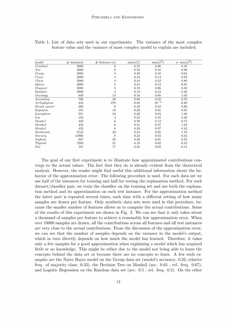
Table 1: List of data sets used in our experiments. The variance of the most complexfeature value and the variance of most complex model to explain are included.

model # instances # features (n) max(σ2i ) max(σ2) n· max(σ2)

CondInd 2000 8 0.25 0.06 0.48Xor 2000 6 0.32 0.16 0.96Group 2000 4 0.30 0.16 0.64Cross 2000 4 0.43 0.14 0.92Chess 2000 4 0.44 0.22 0.88Sphere 2000 5 0.21 0.13 0.65Disjunct 2000 5 0.10 0.06 0.30Random 2000 4 0.19 0.12 0.48Oncology 849 13 0.16 0.08 1.04Annealing 798 38 0.08 0.02 0.76Arrhythymia 452 279 0.03 10−3 0.28Breast cancer 286 9 0.22 0.10 0.90Hepatitis 155 19 0.20 0.05 0.95Ionosphere 351 34 0.20 0.04 1.36Iris 150 4 0.23 0.10 0.40Monks1 432 6 0.29 0.12 0.72Monks2 432 6 0.31 0.27 1.62Monks3 432 6 0.20 0.07 0.42Mushroom 8124 22 0.24 0.05 1.10Nursery 12960 8 0.22 0.03 0.24Soybean 307 35 0.20 0.01 0.35Thyroid 7200 21 0.18 0.02 0.42Zoo 101 17 0.25 0.02 0.14

The goal of our first experiment is to illustrate how approximated contributions con-verge to the actual values. The fact that they do is already evident from the theoreticalanalysis. However, the reader might find useful this additional information about the be-havior of the approximation error. The following procedure is used. For each data set weuse half of the instances for training and half for testing the explanation method. For eachdataset/classifier pair, we train the classifier on the training set and use both the explana-tion method and its approximation on each test instance. For the approximation methodthe latter part is repeated several times, each time with a different setting of how manysamples are drawn per feature. Only synthetic data sets were used in this procedure, be-cause the smaller number of features allows us to compute the actual contributions. Someof the results of this experiment are shown in Fig. 2. We can see that it only takes abouta thousand of samples per feature to achieve a reasonably low approximation error. Whenover 10000 samples are drawn, all the contributions across all features and all test instancesare very close to the actual contributions. From the discussion of the approximation error,we can see that the number of samples depends on the variance in the model’s output,which in turn directly depends on how much the model has learned. Therefore, it takesonly a few samples for a good approximation when explaining a model which has acquiredlittle or no knowledge. This might be either due to the model not being able to learn theconcepts behind the data set or because there are no concepts to learn. A few such ex-amples are the Naive Bayes model on the Group data set (model’s accuracy: 0.32, relativefreq. of majority class: 0.33), the Decision Tree on Monks2 (acc. 0.65 , rel. freq. 0.67),and Logistic Regression on the Random data set (acc. 0.5 , rel. freq. 0.5). On the other

12


log10(samples per feature)

abso

lute

err

or

0.05

0.10

1 2 3 4

condInd NB group NB

1 2 3 4

monks2 ANN monks2 DT

random ANN

1 2 3 4

random logREG sphere bstDT

1 2 3 4

0.05

0.10

sphere DT

99%maxmean

Figure 2: Mean, 99th-percentile, and maximum errors for several dataset/classifier pairsand across different settings of how many samples are drawn per feature. Notethat the error is the absolute difference between the approximated and actualcontribution of a feature’s value. The maximum error is the largest such observeddifference across all instances.

hand, if a model successfully learns from the data set, it requires more samples to explain.For example, Naive Bayes on CondInd (acc. 0.92 , rel. freq. 0.50) and a Decision Tree onSphere (acc. 0.80 , rel. freq. 0.50). In some cases a model acquires incorrect knowledge orover-fits the data set. One such example is the ANN model, which was allowed to over-fitthe Random data set (acc. 0.5 , rel. freq. 0.5). In this case the method explains what themodel has learned, regardless of whether the knowledge is correct or not. And although theexplanations would not tell us much about the concepts behind the data set (we concludefrom the model’s performance, that it’s knowledge is useless), they would reveal what themodel has learned, which is the purpose of an explanation method.

In our second experiment we measure sample variances and classification running times.These will provide insight into how much time is needed for a good approximation. Weuse the same procedure as before, on all data sets, using only the approximation method.We draw 50000 samples per feature. Therefore, the total number of samples for eachdataset/classifier pair is: 50000n times the number of test instances, which is sufficient fora good estimate of classification times and variances. The maximum σ2

i in Table 1 revealthat the crisp features of synthetic data sets have higher variance and are more difficultto explain than features from real-world data sets. Explaining the prediction of the ANNmodel for an instance Monks2 is the most complex explanation (that is, requires the mostsamples - see Fig. 2), which is understandable given the complexity of the Monks2 concept

13


row

colu

mn

logREG

NB

DT

RF

SVM

bstDT

bstNB

ANN

iris

(4)

rand

om (

4)

mon

ks2

(6)

grou

p (4

)

disj

unct

(5)

cros

s (4

)

ches

s (4

)

xor

(6)

mon

ks3

(6)

mon

ks1

(6)

brea

st c

ance

r (9

)

cond

Ind

(8)

sphe

re (

5)

nurs

ery

(8)

zoo

(17)

hepa

titis

(19

)

onco

logy

(13

)

thyr

oid

(21)

mus

hroo

m (

22)

anne

alin

g (3

8)

soyb

ean

(35)

iono

sphe

re (

34)

arrh

ythm

ia (

279)

<1sec

<5sec

<10sec

<1min

<5min

>5min

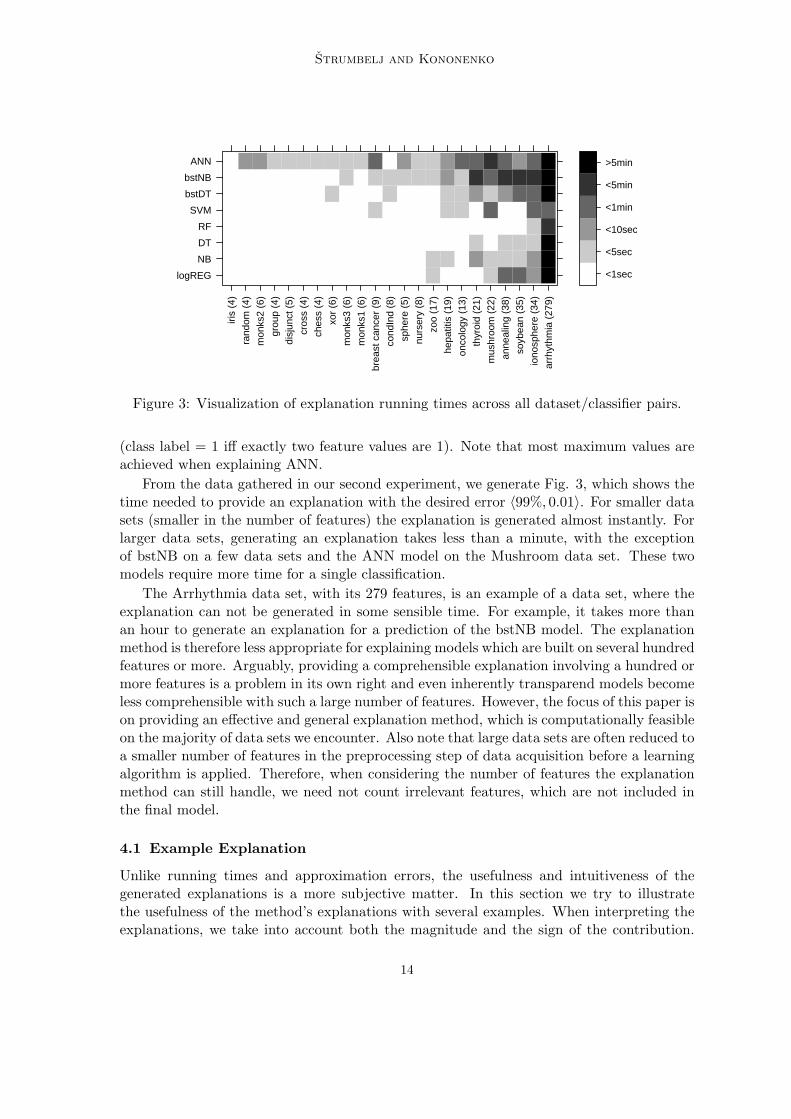
Figure 3: Visualization of explanation running times across all dataset/classifier pairs.

(class label = 1 iff exactly two feature values are 1). Note that most maximum values areachieved when explaining ANN.

From the data gathered in our second experiment, we generate Fig. 3, which shows thetime needed to provide an explanation with the desired error 〈99%, 0.01〉. For smaller datasets (smaller in the number of features) the explanation is generated almost instantly. Forlarger data sets, generating an explanation takes less than a minute, with the exceptionof bstNB on a few data sets and the ANN model on the Mushroom data set. These twomodels require more time for a single classification.

The Arrhythmia data set, with its 279 features, is an example of a data set, where theexplanation can not be generated in some sensible time. For example, it takes more thanan hour to generate an explanation for a prediction of the bstNB model. The explanationmethod is therefore less appropriate for explaining models which are built on several hundredfeatures or more. Arguably, providing a comprehensible explanation involving a hundred ormore features is a problem in its own right and even inherently transparend models becomeless comprehensible with such a large number of features. However, the focus of this paper ison providing an effective and general explanation method, which is computationally feasibleon the majority of data sets we encounter. Also note that large data sets are often reduced toa smaller number of features in the preprocessing step of data acquisition before a learningalgorithm is applied. Therefore, when considering the number of features the explanationmethod can still handle, we need not count irrelevant features, which are not included inthe final model.

4.1 Example Explanation

Unlike running times and approximation errors, the usefulness and intuitiveness of thegenerated explanations is a more subjective matter. In this section we try to illustratethe usefulness of the method’s explanations with several examples. When interpreting theexplanations, we take into account both the magnitude and the sign of the contribution.

14


(a) NB model (b) bstDT model

Figure 4: The boosting model correctly learns the concepts of the Monks1 data set, whileNaive Bayes does not and misclassifies this instance.

If a feature-value has a larger contribution than another it has a larger influence on themodel’s prediction. If a feature-value’s contribution has a positive sign, it contributestowards increasing the model’s output (probability, score, rank, ...). A negative sign, onthe other hand, means that the feature-value contributes towards decreasing the model’soutput. An additional advantage of the generated contributions is that they sum up to thedifference between the model’s output prediction and the model’s expected output, givenno information about the values of the features. Therefore, we can discern how much themodel’s output moves when given the feature values for the instance, which features areresponsible for this change, and the magnitude of an individual feature-value’s influence.These examples show how the explanations can be interpreted. They were generated forvarious classification models and data sets, to show the advantage of having a generalexplanation method.

The first pair of examples (see Fig. 4) are explanations for an instance from the firstof the well-known Monks data sets. For this data set the class label is 1 iff attr1 and attr2are equal or attr5 equals 1. The other 3 features are irrelevant. The NB model, due to itsassumption of conditional independence, does not learn the importance of equality betweenthe first two features and misclassifies the instance. However, both NB and bstDT learnthe importance of the fifth feature and explanations reveal that value 2 for the fifth featurespeaks against class 1.

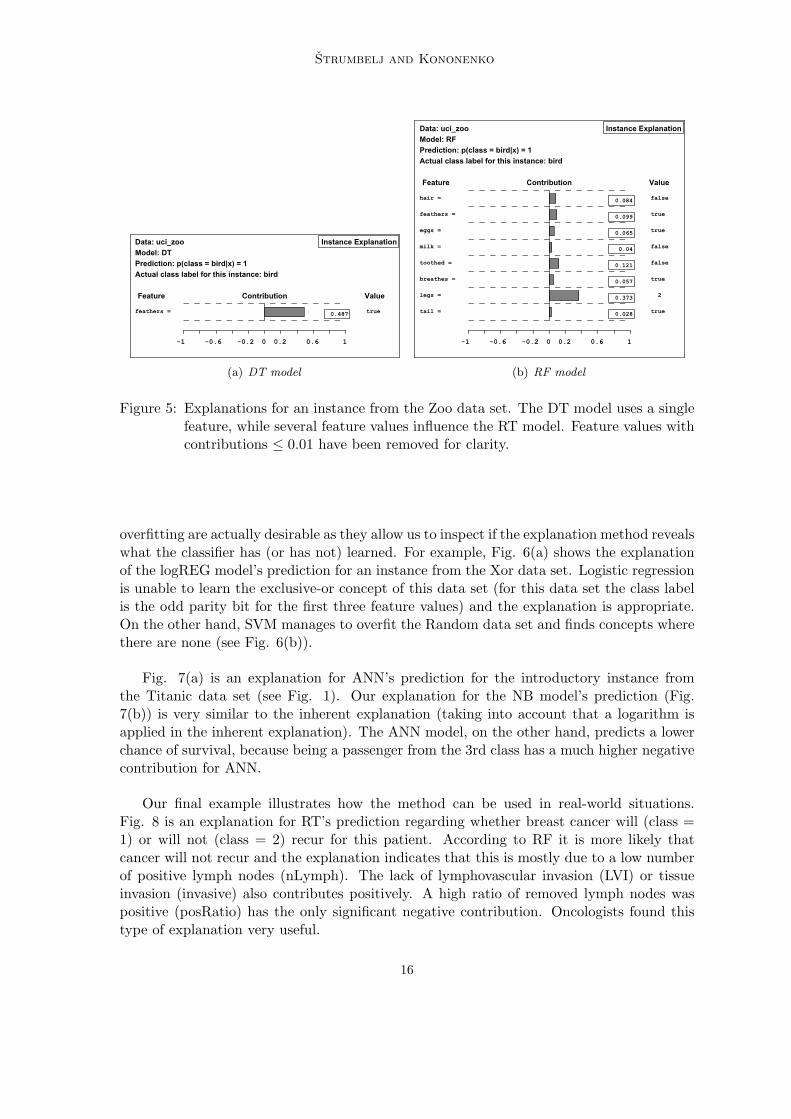
The second pair of examples (see Fig. 5) is from the Zoo data set. Both models predictthat the instance represents a bird. Why? The explanations reveal that DT predicts thisanimal is a bird, because it has feathers. The more complex RF model predicts its a bird,because it has two legs, but also because the animal is toothless, with feathers, withouthair, etc... These first two pairs of examples illustrate how the explanations reflect whatthe model has learnt and how we can compare explanations from different classifiers.

In our experiments we are not interested in the prediction quality of the classifiers and donot put much effort into optimizing their performance. Some examples of underfitting and

15


(a) DT model (b) RF model

Figure 5: Explanations for an instance from the Zoo data set. The DT model uses a singlefeature, while several feature values influence the RT model. Feature values withcontributions ≤ 0.01 have been removed for clarity.

overfitting are actually desirable as they allow us to inspect if the explanation method revealswhat the classifier has (or has not) learned. For example, Fig. 6(a) shows the explanationof the logREG model’s prediction for an instance from the Xor data set. Logistic regressionis unable to learn the exclusive-or concept of this data set (for this data set the class labelis the odd parity bit for the first three feature values) and the explanation is appropriate.On the other hand, SVM manages to overfit the Random data set and finds concepts wherethere are none (see Fig. 6(b)).

Fig. 7(a) is an explanation for ANN’s prediction for the introductory instance fromthe Titanic data set (see Fig. 1). Our explanation for the NB model’s prediction (Fig.7(b)) is very similar to the inherent explanation (taking into account that a logarithm isapplied in the inherent explanation). The ANN model, on the other hand, predicts a lowerchance of survival, because being a passenger from the 3rd class has a much higher negativecontribution for ANN.

Our final example illustrates how the method can be used in real-world situations.Fig. 8 is an explanation for RT’s prediction regarding whether breast cancer will (class =1) or will not (class = 2) recur for this patient. According to RF it is more likely thatcancer will not recur and the explanation indicates that this is mostly due to a low numberof positive lymph nodes (nLymph). The lack of lymphovascular invasion (LVI) or tissueinvasion (invasive) also contributes positively. A high ratio of removed lymph nodes waspositive (posRatio) has the only significant negative contribution. Oncologists found thistype of explanation very useful.

16


(a) logREG model (b) SVM model

Figure 6: The left hand side explanation indicates that the feature values have no signifi-cant influence on the logREG model on the Xor data set. The right hand sideexplanation shows how SVM overfits the Random data set.

(a) ANN model (b) NB model

Figure 7: Two explanations for the Titanic instance from the introduction. The left handside explanation is for the ANN model. The right hand side explanation is forthe NB model.

17


Figure 8: An explanation or the RF model’s prediction for a patient from the Oncologydata set.

5. Conclusion

In the introductive section, we asked if an efficient and effective general explanation methodfor classifiers’ predictions can be made. In conclusion, we can answer yes. Using only theinput and output of a classifier we decompose the changes in its prediction into contribu-tions of individual feature values. These contributions correspond to known concepts fromcoalitional game theory. Unlike with existing methods, the resulting theoretical propertiesof the proposed method guarantee that no matter which concepts the classifier learns, thegenerated contributions will reveal the influence of feature values. Therefore, the methodcan effectively be used on any classifier. As we show on several examples, the method canbe used to visually inspect models’ predictions and compare the predictions of differentmodels.

The proposed approximation method successfully deals with the initial exponential timecomplexity, makes the method efficient, and feasible for practical use. As part of furtherwork we intend to research whether we can efficiently not only compute the contributions,which already reflect the interactions, but also highlight (at least) the most importantindividual interactions as well. A minor issue left to further work is extending the approxi-mation with an algorithm for optimizing the number of samples we take. It would also beinteresting to explore the possibility of applying the same principles to the explanation ofregression models.

References

R. Andrews, J. Diederich, and A. B. Tickle. Survey and critique of techniques for extractingrules from trained artificial neural networks. Knowledge-Based Systems, 8:373–389, 1995.

18


Artur Asuncion and David J. Newman. UCI Machine Learning Repository, http://www.ics.uci.edu/~mlearn/MLRepository.html, 2009.

Barry Becker, Ron Kohavi, and Dan Sommerfield. Visualizing the simple bayesian classier.In KDD Workshop on Issues in the Integration of Data Mining and Data Visualization,1997.

Leo Breiman. Random forests. Machine Learning Journal, 45:5–32, 2001.

Javier Castro, Daniel Gomez, and Juan Tejada. Polynomial calculation of the shapleyvalue based on sampling. Computers and Operations Research, 2008. (in print, doi:10.1016/j.cor.2008.04.004).

Shay Cohen, Gideon Dror, and Eytan Ruppin. Feature selection via coalitional game theory.Neural Computation, 19(7):1939–1961, 2007.

Lutz Hamel. Visualization of support vector machines with unsupervised learning. In Com-putational Intelligence in Bioinformatics and Computational Biology, pages 1–8. IEEE,2006.

Aleks Jakulin, Martin Mozina, Janez Demsar, Ivan Bratko, and Blaz Zupan. Nomogramsfor visualizing support vector machines. In KDD ’05: Proceeding of the eleventh ACMSIGKDD international conference on Knowledge discovery in data mining, pages 108–117, New York, NY, USA, 2005. ACM. ISBN 1-59593-135-X.

Alon Keinan, Ben Sandbank, Claus C. Hilgetag, Isaac Meilijson, and Eytan Ruppin. Fairattribution of functional contribution in artificial and biological networks. Neural Com-putation, 16(9):1887–1915, 2004.

Ron Kohavi and George H. John. Wrappers for feature subset selection. Artificial Intelli-gence journal, 97(1–2):273–324, 1997.

Igor Kononenko. Machine learning for medical diagnosis: history, state of the art andperspective. Artificial Intelligence in Medicine, 23:89–109, 2001.

Igor Kononenko and Matjaz Kukar. Machine Learning and Data Mining: Introduction toPrinciples and Algorithms. Horwood publ., 2007.

Vincent Lemaire, Raphael Fraud, and Nicolas Voisine. Contact personalization using a scoreunderstanding method. In International Joint Conference on Neural Networks (IJCNN),2008.

David Martens, Bart Baesens, Tony Van Gestel, and Jan Vanthienen. Comprehensible creditscoring models using rule extraction from support vector machines. European Journal ofOperational Research, 183(3):1466–1476, 2007.

Stefano Moretti and Fioravante Patrone. Transversality of the shapley value. TOP, 16(1):1–41, 2008.

19


Martin Mozina, Janez Demsar, Michael Kattan, and Blaz Zupan. Nomograms for visu-alization of naive bayesian classifier. In PKDD ’04: Proceedings of the 8th EuropeanConference on Principles and Practice of Knowledge Discovery in Databases, pages 337–348, New York, NY, USA, 2004. Springer-Verlag New York, Inc. ISBN 3-540-23108-0.

Richi Nayak. Generating rules with predicates, terms and variables from the pruned neuralnetworks. Neural Networks, 22(4):405–414, 2009.

Francois Poulet. Svm and graphical algorithms: A cooperative approach. In Proceedings ofFourth IEEE International Conference on Data Mining, pages 499–502, 2004.

Marko Robnik-Sikonja and Igor Kononenko. Explaining classifications for individual in-stances. IEEE Transactions on Knowledge and Data Engineering, 20:589–600, 2008.

Lloyd S. Shapley. A Value for n-person Games, volume II of Contributions to the Theoryof Games. Princeton University Press, 1953.

Duane Szafron, Brett Poulin, Roman Eisner, Paul Lu, Russ Greiner, David Wishart, AlonaFyshe, Brandon Pearcy, Cam Macdonell, and John Anvik. Visual explanation of evidencein additive classifiers. In Proceedings of Innovative Applications of Artificial Intelligence,2006.

Geoffrey Towell and Jude W. Shavlik. Extracting refined rules from knowledge-based neuralnetworks, machine learning. Machine Learning, 13:71–101, 1993.

Erik Strumbelj, Igor Kononenko, and Marko Robnik Sikonja. Explaining instance classifi-cations with interactions of subsets of feature values. Data & Knowledge Engineering, 68(10):886–904, 2009.

20

An Efficient Explanation of Individual Classifications using Game Theory

Documents

Transcript of An Efficient Explanation of Individual Classifications using Game Theory