ISSN: 1439-2305

Number 337 – January 2018

AN ECONOMIC THEORY OF

DEPRESSION AND ITS IMPACT ON

HEALTH BEHAVIOR AND LONGEVITY

Holger Strulik

An Economic Theory of Depression and its Impact on

Health Behavior and Longevity∗

Holger Strulik†

January 2018.

Abstract. In this paper, I introduce depression to the economics of human health

and aging. Based on studies from happiness research, depression is conceptualized

as a drastic loss of utility and value of life (life satisfaction) for unchanged funda-

mentals. The model is used to explain how untreated depression leads to unhealthy

behavior and adverse health outcomes: depressed individuals are predicted to save

less, invest less in their health, consume more unhealthy goods, and exercise less. As

a result, they age faster and die earlier than non-depressed individuals. I calibrate

the model for an average American and discus the socioeconomic gradient of health

and depression as well as the hump-shaped association of antidepressant use with

age. Delays in treatment for depression in young adulthood are predicted to have

significant repercussions on late-life health outcomes and longevity.

Keywords: depression, depression therapy, health behavior, aging, longevity.

JEL: D15, D91, I10, I12.

∗ I would like to thank Gustav Feichtinger, Sophia Khan, Alexia Prskawetz, Miguel Sanchez-Romero, andTimo Trimborn for helpful comments and discussion.

† University of Goettingen, Department of Economics, Platz der Goettinger Sieben 3, 37073 Goettingen,Germany; email: holger.strulik@wiwi.uni-goettingen.de.

The first thing that goes is happiness. You cannot gain pleasure from

anything. That’s famously the cardinal symptom of major depression.

(Solomon, 2015).

1. Introduction

In health economic theory, depression has received relatively little attention. This is perhaps

surprising given the seriousness of the disease. According to the WHO (2017), more than 300

million people worldwide are living with depression, which makes depression the leading cause

of ill health and disability. Depressive disorders are estimated to be responsible of 50 million

years lived with disability, which accounts for 7.5% of the total number of years lived with

disability (WHO, 2017). In the US, 6.7 percent of all adults above age 18 have had at least

one major depressive episode in the past year (NSDUH, 2016). Similar population shares are

observed in other developed countries. In many developing countries, the prevalence is higher

since depression is associated with poverty (Lorant et al., 2003; Strulik, 2018b).

The most notable feature of depression is its strong and independent influence on life satis-

faction, even when controlling for poverty, unemployment, and ill health (Clark et al., 2017).

In fact, mental illness has been identified as the single largest determinant of misery, i.e. of

being in the bottom quarter of the population in terms of life satisfaction, more important than

physical health, income, and unemployment (Layard, 2013). The present research is inspired by

these observations from happiness studies. Building on this literature, I consider the empirical

observation of life satisfaction from surveys as a reasonable approximation of lifetime utility

(Frey and Stutzer, 2002; Clark et al., 2008; Stevenson and Wolfers, 2008).1 I then conceptualize

depression as an exogenous drastic and sustained drop in experienced instantaneous utility and

thus also in lifetime utility (life satisfaction).2

Depression can be treated with drugs or psychotherapy but the efficacy of treatment is imper-

fect and individual-specific. For major depression, it has been estimated that pharmacological

treatment leads to recovery within four months in over 50% of cases. The probability of relapse

1Most of the economics literature uses the terms happiness and life satisfaction interchangeably but it hasbeen argued that the term happiness better describes the instantaneous component of subjective well-being whilelife satisfaction is the more appropriate measure of its evaluative, long-term component (Deaton, 2008; Stevensonand Wolfers, 2008).

2Actually, depression may be triggered by a life event and then persists after the cause has gone. In thispaper, I ignore this refinement in the sequence of events and treat the loss of utility as being fully exogenous.This is a useful device in order to identify causality. In Strulik (2018b), I considered childbirth in poverty as oneparticular trigger of (maternal) depression.

1

into depression, however, remains high unless drugs are continued to be taken (Layard, 2013).

Here, I model depression treatment as medical expenditure that dampens the loss of utility.

Historically, treatment of mental health conditions had been covered less generously than phys-

ical illness by private insurance, a feature, which perhaps contributed to the under-treatment of

mental health problems. In the U.S., it is estimated that one-third of the depressed population

remains untreated (SAMHSA, 2002).

This paper focusses on the impact of depression on health behavior, aging, and longevity.

Depression is associated with less healthy life styles in many dimensions. The rate of daily

cigarette use, for example, is almost twice as high among adults with major depression compared

to the general population (29.7 percent vs. 16 percent; NSDUH, 2006). Depressed individuals are

also more likely to drink heavily and to use other addictive substances (NSDUH, 2006). Aside

from increased alcohol and cigarette consumption, depression is also associated with inactivity,

eating and sleeping problems, and a lack of treatment adherence for medical problems (Schulz

et al., 2002). According to the model proposed in this paper, these behavioral changes are

explained as a direct consequence of reduced life satisfaction. Facing low lifetime utility (life

satisfaction), depressed individuals have less incentive to reduce unhealthy consumption, to save

for health care expenditure in old age, and to invest in their health in monetary terms and

physical exercise. As a result, their bodies age faster and their life ends prematurely. With

respect to unhealthy consumption, for example, the model captures the notion that the high

rate of smoking among depressed people does not reflect a particular preference for nicotine

but a “general self-destructiveness among people for whom the future is only bleak” (Solomon,

2015).

It is well-known that (severe) depression is associated with an increased risk of suicide (ASS,

2014). In this paper, we assume that depression is mild enough such that depressed individuals

do not kill themselves. Formally, we assume that the value of life of depressed individuals is low

but still positive. This allows us to ignore mortality from suicide and to focus on the impact of

depression on mortality through increased morbidity and the speed of aging. Many studies have

documented an association between health and depression. One of the most robust findings is

the relation between depression and cardiovascular disease (Schulz et al., 2002). With regard

to the health deficit index, which is the measure of health used in the present study, Lohman

et al. (2015) document a positive association between depression and the health deficit index

2

in late life, and Rao et al. (2016) find that depression significantly predicts increased health

deficits, disability, and mortality among the elderly.3 A rare study that estimated the impact

of depression on life expectancy is provided by Zivin et al. (2012) who found that depressed

male patients died about 4.8 years earlier than non-depressed patients (71.1 versus 75.9 years).

Saint Onge et al. (2014) also documented an association of major depression and (non-suicide)

mortality risk in the noninstitutionalized U.S. population and found that adjusting for health

behaviors reduces the hazard rate between major depression and mortality by 17%.

In order to investigate health behavior and health outcomes, I integrate the theory of de-

pression into the context of the health deficit model of Dalgaard and Strulik (2014) and extend

the model with unhealthy consumption and physical exercise. The health deficit model has a

foundation in gerontology and predicts that the pace of aging increases as people get older. Most

importantly, health deficits are easily measured by a straightforward metric, the health deficit

index (or frailty index; Mitnitski et al., 2002a,b, 2005; Rockwood et al., 2007; Harttgen et al.,

2013). This allows for a calibration of the model with real data such that the model can be

used to quantitatively address lifetime health issues of depression. This feature distinguishes

the health deficit approach from the earlier paradigm in health economics, the accumulation

of health capital (Grossman, 1972), which considered a latent variable that remained unknown

in medical science. Conceptually, the main distinctive feature of the health deficit approach

is the implication that unhealthy people age faster. The health capital model, in contrast, as-

sumes that healthy people age faster (lose more health capital through depreciation). Among

other things, this counterfactual assumption implies that the health capital model predicts that

early-life health shocks matter little for late-life health outcomes (for a critique, see Almond and

Currie, 2011) whereas the health deficit model predicts the opposite (Dalgaard et al., 2017).

In the current context, this distinction matters because the health deficit model highlights the

importance of early diagnosis and treatment of mental illness, a feature that would be impossible

to observe within the health capital paradigm.4

3The health deficit index (or frailty index) computes the percentage of health deficits present in a person froma long list of potential health deficits, see Mitnitski et al. (2002a,b; 2005); and Rockwood and Mitnitski (2006,2007).

4 Earlier studies using the health deficit model were concerned with the long-term evolution of the age atretirement (Dalgaard and Strulik, 2017), adaptation to poor health (Schuenemann et al., 2017a), the gender gapin mortality (Schuenemann et al., 2017b), and the education gradient (Strulik, 2018a).

3

The modeling of depression treatment implements (for the first time) the suggestion to analyt-

ically discuss the use of antidepressants as a new form of consumption that lies in the currently

grey area between medication and consumer goods. (Katolik and Oswald, 2017, Blanchflower

and Oswald, 2016). It is related to a small literature arguing in favor of a backward causality

from happiness to (economic) behavior. Guven (2012) identifies the backward causality by in-

strumenting happiness with unexpected sunshine and finds that happier people save more, have

a lower marginal propensity to consume, and expect a longer life. Similarly, De Neve et al.

(2013) find that high subjective wellbeing is associated with healthier eating, reduced likelihood

of smoking, more exercise, and a longer life.

So far, two alternative and potentially complementing theories of depression have been sug-

gested. De Quidt and Haushofer (2016) propose to model depression symptoms as the conse-

quence of downward shocks in the belief about the return to effort in a model where a decision-

maker chooses labor effort, non-food consumption, food consumption, and sleep. Health issues

and their consequences on life cycle-health and longevity are not addressed. Strulik (2018b)

proposes an overlapping generations model to address the intergenerational transmission of de-

pression and shows that this gene-environment interaction may generate a poverty trap. The

study focused on maternal depression modeled in reduced-form as increased present-bias, which

leads to less child investments of depressed mothers. Health behavior and its life cycle implica-

tions are not addressed.

This paper is organized as follows. In the next section, I set up a life-cycle model of depres-

sion, health behavior, health outcomes, and longevity; and, using comparative statics, I derive

analytical results for the use of antidepressants at the intensive and extensive margins. The full

dynamic model can only be analyzed numerically. In Section 3, I calibrate the model for a refer-

ence American (a 20-year-old male in the year 2000) and in Section 4, I assess the quantitative

impact of depression and depression treatment on life-cycle behavior, health, and longevity. In

Section 5, I consider applications and extensions of the basic model with regard to depression

and the income gradient of health and longevity, feedback effects of depression on labor market

outcomes (retirement and lifetime earnings), the impact of delayed diagnosis and treatment on

health outcomes, and a u-shaped age-pattern of depression in a population with idiosyncratic

susceptibility to depression. Section 6 concludes with suggestions for future research.

4

2. A Theory of Depression, Health Behavior, and Health Outcomes

2.1. Utility. Consider an individual who derives utility from the consumption of health-neutral

goods c and unhealthy goods u and whose utility declines in the number of health deficitsD. The

(sub-)utility function U(c, u,D) exhibits, as usual, declining marginal utility from consumption,

∂U/∂j > 0, ∂2/∂j2 < 0 for j = c, u. Health deficits reduce utility and, following Finkelstein

et al. (2013), we assume that health deficits reduce the marginal utility from consumption,

∂2U/(∂c∂D) < 0. Additionally, individuals may engage in healthy behavior and the exerted

health effort x, which could be thought of as physical exercise, has a utility cost (e.g. in terms of

leisure). The disutility from effort increases in the number of health deficits present in a person.

For simplicity, we assume that the subutility function for the cost of health effort f(x,D) is

separable from the utility from consumption and has positive first derivatives and non-positive

second derivatives.

As motivated in the Introduction, depression can be best conceptualized as a downward-shifter

of the utility function. The severity of the depression is measured by δ ≥ 0. In this paper,

we focus on depression that is mild enough such that utility remains positive and depressed

individuals are not induced to kill themselves. Instead, we investigate the effects of depression

on longevity through induced unhealthy behavior and (in the extended model) through the side-

effects of medication and addiction. When the depression is treated, the negative utility shock

becomes less severe. A unit of treatment m could be conceptualized as the use of prescription

antidepressants or therapy. The efficacy of the treatment is denoted by η ≥ 0. Together, this

means that the utility of depressed individuals is reduced by δg(m, η) with ∂g/∂η < 0 and with

declining returns of treatment intensity, ∂g/∂m < 0, ∂2g/∂m2 > 0. Moreover, an extra unit of

treatment reduces depression to a larger degree when treatment is effective, i.e. ∂2g/∂η∂m < 0.

Reasonable albeit not decisive further assumptions are that g(0, η) = 1 and lim gm→∞ = 0. The

first assumption means that untreated individuals experience the full power of depression δ.

The second assumption rules out that non-depressed individuals take antidepressants to further

boost their happiness. Altogether, this means that lifetime utility is given by

V =

∫ T

0[U(D, c, u)− f(x,D)− δg(m, η)] e−ρtdt, (1)

in which t is age, T is the age at death, and ρ is the time preference rate. Here, we focus

on a deterministic model in which death occurs when an upper limit of health deficits D has

5

been accumulated. As shown in Strulik (2015a) and Schuenemann et al. (2017b), stochastic

versions of the health deficit model in which the probability of death depends positively on

health deficits add more realism at the price of higher complexity but provide little extra insight

into life-cycle choices and outcomes. Since the present model is already quite complex, for the

sake of simplicity, we abstract from stochastic death.

2.2. Health. The state of health is measured by a health deficit index D, defined as the share

of health deficits present in a person (from a long list of potential health deficits). As shown

by Mitnitski et al. (2002), Harttgen et al. (2013), and Abeliansky and Strulik (2017), health

deficits are accumulated in a quasi-exponential way with increasing age. As in Dalgaard and

Strulik (2014) and Schuenemann et al. (2017a), we assume that the “natural” increase of health

deficits can be slowed down by health investment h and accelerated by unhealthy consumption

u. Additionally, we assume that health effort x slows down the accumulation of health deficits.

In short, health deficits accumulate as

D = µ [D −Ahγ +Buω − Exκ − a] , (2)

in which µ is the “natural” force of aging. The parameters A and γ measure the efficacy of

health technology, the parameters B and ω measure the degree of unhealthy consumption, and

the parameters E and κ measure the impact of health effort. We assume decreasing returns of

health investment and health effort, 0 < γ, κ < 1 while marginal health costs are increasing in

unhealthy consumption, ω > 1.

2.3. Wealth. Individuals receive an income flow w, conceptualized as net wage income until

retirement, and as pension income afterwards. Income is used for consumption, saving at interest

rate r, and health expenditure. In order to introduce a primitive health care system, we assume

that a share φ of health investments and a share φm of depression treatments are paid out of

pocket. Let the prices of unhealthy consumption, health investment, and depression treatment

be denoted by q, p, and pm. Then, wealth k accumulates as

k = w + rk − c− qu− pφh− pmφmm. (3)

2.4. Solution. Individuals chose consumption (c and u), health expenditure h, health effort x,

and depression treatment m in order to maximize lifetime utility (1) subject to constraints (2)

6

and (3), the initial states of health D(0) and wealth k(0), the boundary conditions D(T ) = D

and k(T ) = k, and non-negativity constraints on all choice variables. However, it will turn out

that only for unhealthy consumption and depression treatment, the non-negativity constraint

becomes occasionally binding whereas the other choices are always positive. The associated

Hamiltonian is given by

H = U(D, c, u)− f(x,D)− δg(m, η)

+ λDµ [D −Ahγ +Buω − Exκ − a] + λk [w + rk − c− pφh− pmφmm] . (4)

The first order conditions for a maximum are:

∂U(D, c, u)

∂c= λk (5)

∂U(D, c, u)

∂u≤ λkq − λDµBωu

ω−1 with = for u > 0 (6)

−λDµγAγ−1 = λkφp (7)

−λDµκExκ−1 =

∂f

∂x(8)

−δ∂g

∂m≤ λkφmpm with = for m > 0. (9)

I have aligned the first order conditions such that the left-hand side always shows the marginal

benefit and the right-hand side shows the marginal cost. Condition (5) requires that the marginal

utility from consumption of health neutral goods equals the marginal cost in terms of foregone

future utility, measured by the shadow price of capital. Condition (6) requires that the marginal

utility from unhealthy consumption is not larger than the marginal cost, which consists of

implied forgone future utility λkq and the marginal impact of unhealthy consumption on health

µBωuω−1, evaluated by the shadow price of health deficits. Notice that future health deficits

are bad such that λD is negative. Condition (7) requires that the marginal return from health

investment µγAγ−1 evaluated with the shadow price of health deficits equals the marginal cost in

terms of foregone marginal utility from consumption. Condition (8) requires that the marginal

return from health effort equals the marginal utility cost of health effort.

Finally, condition (9) requires that the marginal return of depression treatment is not larger

than the marginal cost of treatment. To observe this, recall that treatment reduces depression,

i.e. that ∂g/∂m < 0. For the treated, marginal benefits equal marginal costs. When marginal

7

costs exceed marginal benefits, individuals remain untreated. Inserting (5) into (9), we obtain

the depression treatment constraint:

0 ≤ G ≡∂U(D, c, u)

∂cφmpm + δ

∂g(m, eta)

∂m. (10)

From the inspection of (10), we obtain a first result:

Proposition 1 (Intensive Margin). The treatment intensity of depression m is increasing in

the level of consumption c (and thus income) of the patient, and in the number of health deficits

of the patient. It declines in the price pm of the treatment and the out-of-pocket share φm.

For the proof, I apply the implicit function theorem on (10) evaluated with equality. For

example, we have for price pm, dm/dpm = − (φm∂U(D, c, u)/∂c) /(

δ∂2g/∂m2)

< 0, and like-

wise for φm. The comparative static for health deficits uses the assumption ∂2U/(∂c∂D) < 0

and the comparative static for consumption uses the assumption of declining marginal utility

from consumption ∂2U/(∂c2) < 0. The intuition for the result with respect to consumption

(income) is that individuals who experience little extra utility from spending an extra dollar on

consumption are more inclined to spend income on depression treatment. The marginal utility

from consumption is low when the level of consumption is high or when many health deficits are

present. As long as consumption goods are normal (which we assume), richer individuals will

consume more. In other words, poor individuals have other pressing needs and are therefore less

inclined to spend much money on depression treatment, in particular, if treatment prices are

high and the out-of-pocket share is large (i.e. if they are uninsured).

Proposition 2 (Extensive Margin). Depression remains untreated if the treatment is suffi-

ciently inefficient (η is low), if the out-of-pocket share φm is sufficiently large, or if the level of

consumption (income) of the patient is sufficiently low.

The proof with respect to η shows that G is increasing in η since ∂2g/∂m∂η > 0, which makes

it less likely that (10) binds with equality when η is low. The other comparative statics are

obtained similarly. These comparative statics, however, do not provide any information about

the impact of depression on health behavior and longevity. For this, we need the full solution

of the model, which also requires the costate equations and boundary conditions to be fulfilled.

8

The costate equations are given by

λkr = λkρ− λk (11)

∂U(c, u,D)

∂D−∂f(x,D)

∂D+ λDµ = λDρ− λD (12)

Aside from the boundary conditions on k and D, the optimal solution of the free terminal time

problem also fulfills H(T ) = 0. Inspection of (4) shows that the Hamiltonian assumes a large

value, ceteris paribus, when utility is large, i.e. for individuals who are healthy, wealthy, and

not depressed. The fact that instantaneous utility is strictly concave in the level of consumption

while lifetime utility is (aside from the health effects) linear in instantaneous utility motivates

the pursuit for a long life. Individuals, unconditionally prefer to extend their consumption over

a longer time period against consuming more right now. The pursuit for a long life, however,

comes also at a cost in terms of health investments, health effort, and the eschewal of unhealthy

consumption. Rich individuals experience lower marginal utility from (even more) consumption

and have more funds to finance a long life. They are thus predicted to live longer. These

mechanism were the main subject of investigation in Dalgaard and Strulik (2014). The novelty

here is that depression drives down the level of instantaneous utility (experienced happiness).

This means that it reduces the desire for a long life which in turn reduces the incentive to invest

time and money in health and increases the incentive to indulge in unhealthy consumption.

In order to explore the impact of depression on health and health behavior we need the full

solution of the model, i.e. the dynamic life cycle trajectories implied by the first order conditions

and boundary conditions. This can be achieved only numerically and the first step is to assume

functional forms for the sub-utility functions. For simplicity, we conceptualize total consumption

c as a convex combination of the consumption of health neutral goods and unhealthy goods,

c = θc+(1−θ)u, 0 < θ < 1. One advantage of such a simple additive sub-utility function is that

it allows for a preemptively high price at which households abstain from unhealthy consumption

(see below). We assume that utility from total consumption is iso-elastic. Controlling for health

deficits, utility is given by (c1−σ − 1)/(1 − σ), in which 1/σ is the elasticity of intertemporal

substitution. Following Finkelstein et al. (2013), we treat the state of health as a shifter of the

utility function of consumption such that both utility and marginal utility of consumption are

negatively affected by bad health. Specifically, we assume that health adjusted utility is given

by (D/D0)−ǫ · (c1−σ − 1)/(1− σ). The parameter ǫ controls the amount by which an additional

9

health deficit will shift the utility function downwards. The normalizing constant D0 implies

that at the state of best health (which is the initial level of health deficits), utility is unaffected

by health.

The disutility from health effort (physical exercise) is formalized as f(x,D) = (D/D0)χτx,

with τ > 0 and χ > 1. In order to obtain a closed form solution, we assume that utility is linear

in health effort x. Disutility from effort is potentially increasing in health deficits (χ ≥ 0). Since

D(t) ≥ D0, health effort becomes increasingly painful with the accumulation of health deficits

for χ > 1. The parameter τ controls how much the individual, in general, dislikes health effort.

Finally, we assume a simple exponential function for depression treatment g(m, η) = e−ηm.

This function fulfills the assumption of decreasing returns. It implies that non-depressed in-

dividuals will not demand antidepressants and that non-treated individuals experience the full

power of depression. In short, lifetime utility (1) is parameterized as

V =

∫

∞

0

(

D

D0

)

−ǫ [θc+ (1− θ)u]1−σ− 1

1− σ−

(

D

D0

)χ

τx− δe−ηmdt. (13)

From the first order conditions, we obtain closed form solutions for u, x, and m (see the Ap-

pendix for details on the derivation of these results). The solution for unhealthy consumption

is displayed in (14).

u =

{

[

1−θθ

− q]

Aγhγ−1

Bωφp

}1

ω−1

for q < 1−θθ

0 otherwise.

(14)

For unhealthy consumption to prevail, the relative utility weight of unhealthy goods, (1− θ)/θ,

has to exceed the price q. If unhealthy consumption exists, then condition (14) predicts that its

extent is large if the resulting health damage is low (B is low), if medical efficiency in repairing

damage is large (A is large), or if the price of health goods p is low.

The solution for health effort is displayed in (15).

x =

[

(

D

D0

)

−(ǫ+χ) (c)−σθφpκE

τµAγhγ−1

]1

1−κ

. (15)

Health effort (physical exercise) is high for healthy persons (with low D) and when the health

gain E is large. It is low when τ is large, i.e. when exercising provides much disutility. Physical

exercise is also high when the marginal return of health investments γAhγ−1/p is low. This

outcome is intuitive because it makes sense to exercise more in order to reduce the accumulation

10

of health deficits when there is little return to further monetary investments on the state of

health.

The solution for depression treatment is displayed in (16). The comparative statics stated in

general form in Proposition 1 and 2 are easily verified by inspection of (16).

m = max

{

0,1

ηlog

[

δη(D/D0)ǫcσ

pmφmθ

]}

. (16)

Finally, the optimal solution is characterized by two dynamic equations for consumption and

health expenditure (see Appendix for details on the derivation):

˙c

c=

1

σ

[

r − ρ− ǫ

(

D

D

)]

, (17)

h

h=

1

1− γ

{

r − µ−

[

ǫc1−σ − 1

1− σ+ xτ

(

D

D0

)χ+ǫ]

µAγhγ−1cσ

pφD

}

. (18)

Equation (17) shows the standard Euler equation for consumption adjusted by health deficits,

Intuitively, the accumulation of health deficits drives down the incentive to spend on consump-

tion in old age, and thus lowers the slope of the lifetime consumption path (which may become

hump-shaped; see Strulik, 2015b). Equation (18) shows the health-Euler equation. When health

does not show up in the utility function (ǫ = τ = 0), health expenditure becomes steeper with

rising return on wealth and declining force of mortality (i.e. with greater incentive to save for

late-life health expenditure). The presence of health deficits in the utility function decreases the

slope of the health expenditure path through its impact on the utility from consumption and on

the disutility from exerting health effort.

3. Calibration

The model is calibrated, as in Dalgaard and Strulik (2014), for an average white 20-year-old

American male in the year 2000. From Mitnitski et al. (2002a), we take the estimate of for

the rate of aging, µ = 0.043, and from Dalgaard and Strulik (2014), we take r = ρ = 0.06.

From age 20 to 65, we set w = 35, 320, which is the average annual pay for workers in the year

2000 (BLS, 2011). For older individuals, we set w = 0.45 · 35, 320 using an average replacement

rate of 0.45 from the OECD (2016). We assume that individuals neither bequeaths nor inherit

any wealth, k0 = k = 0. We set the out-of-pocket expenditure share to φ = 0.28 for all ages.

This proxy somewhat overestimates the out-of-pocket share of the elderly and underestimates it

11

somewhat for the young (Machlin and Carper, 2014). For the benchmark run, we set φm = φ,

assuming no discrimination of payments for depression treatment. Furthermore, we normalize

prices p = q = 1. This is an interesting benchmark case because it eliminates any price channel

through which poor individuals may have an incentive to consume more unhealthy goods or

spend less on general health care.

The calibration of the effect of health on utility is related to Finkelstein et al. (2013) who

estimate that a one-standard-deviation increase in the number of chronic diseases is associated

with a 11% decline in the marginal utility of consumption (with a 95% confidence band from

2.7% to 16.8%). Finkelstein et al. focus on individuals above 50 and apply a smaller set of

more severe health deficits compared to this study. Here, we calibrate the frailty index of

Mitnitski et al. (2002a), which also contains relatively mild health deficits like farsightedness

and incontinence. We thus consider, for the benchmark case, a smaller impact of health deficits

by setting ǫ = 0.06. This means that an unexpected increase in health deficits from D0 by one

standard deviation reduces the marginal utility from consumption by 4 percent.

Since most of the available empirical literature on consumption of unhealthy goods is on

cigarettes and tobacco, we conceptualize u as smoking. On average, Americans spent $ 319 on

cigarettes in the year 2000 (BLS, 2002). The Smoking intensity declines with age, at least from

middle age onwards (Holford et al., 2014). Empirically, there is some variation in the estimates

of years of life lost due to smoking, ranging from 2.5 years (Preston et al., 2010) to 10 years

(Jha et al., 2013). Here, we try to fit an intermediate value of 4.3 years, estimated by a study

that takes selection into smoking into account, see Darden et al., 2015.

To measure physical exercise, we use the metric of metabolic equivalents (METs) defined as

the energy cost of a given physical activity divided by energy expenditure at rest. This metric

allows for the aggregation of different physical activities like walking, playing sports, gardening,

etc., and to compare them across individuals and ages. The average American in Moore et

al.’s (2012) sample spends about 1.14 MET per day (8 MET per week) on physical exercise, an

equivalent of about 23 minutes of brisk walking per day. Moore et al. estimate that this exercise

increases life expectancy by about 3 years. They also document strongly decreasing returns from

physical exercise, i.e. large gains for departure from inactivity and very small gains for excessive

exercise. Studies from the UK (Townsend et al., 2015) and Canada (Statistics Canada, 2007)

suggest that the intensity of exercise declines by about a factor of 2 from age 35 to age 70.

12

Assuming that British and Canadian men are, in this regard, sufficiently similar to Americans,

we try to match their age gradient of physical activity.

To summarize, the remaining parameters of the model for a non-depressed individual, that is

A, a, B, E, γ, χ, θ, σ, τ , and ω, are estimated to fit the following stylized facts: a 20-year-old

U.S. American male in the year 2000 has a life expectancy of 55.5 years (dying at age 75.5; NVSS,

2012), total spending on health, on average, equals 13 percent of his lifetime income (the health

expenditure share of GDP in the U.S. in the year 2000; World Bank, 2015); as the individual

ages, health expenditure increases by about two percent per year (Dalgaard and Strulik, 2014);

the individual spends, on average, $ 300 per year on smoking; smoking expenditure declines by

50 percent from age 30 to age 60; smoking costs 4.3 years of life; the individual spends x = 1.14

METs per day on exercise, which allows him to live 3 years longer than he would in total

inactivity; and such that we map – with successive out-of-sample predictions – the age gradient

as well as the marginal return of physical exercise for alternative x, as estimated by Moore et

al. (2012). This leads to the estimates A = .00013, a = 0.0182, B = 9.5 · 10−7, E = 1.06 · 10−3,

γ = .32, χ = 1.15, κ = 0.1, θ = .073, σ = 1.08, τ = 0.0085, and ω = 1.20. While most of these

parameters are latent, there exist many studies on the size of σ. The estimated value accords

well with studies suggesting that the intertemporal elasticity of substitution is close to unity

(Chetty, 2006).

As another plausibility check of the calibration, we compute the value of life (VOL) of the

Reference American and compare it with previous estimates. The VOL provides a monetary

expression of aggregate utility experienced during life until its end, that is, utility is converted

by the unit value of an “util”, u′(c). The VOL at the initial age is obtained by applying the

formula V OL = V/[∂u(c(0), u(0), D0)/∂c(0)]. The benchmark calibration predicts a VOL of

about $ 6.7 million at age 20. In terms of order of magnitude, this value corresponds well to

Murphy and Topel’s (2006, Fig. 3) estimate of a VOL of about $ 6.5 million for American men

at age 20.

Most studies on the toll of depression on longevity compute mortality hazard rates for small

samples because computation of effects on life expectancy needs large sample sizes. Such a study

is provided by Zivin et al. (2012) who use data from the U.S. department of Veteran Affairs and

the National Death Index and find that depressed individuals died, on average, at age 71.1 while

average non-depressed individuals died at age 75.9. While the sample is not representative, the

13

leading causes of death were similar to those of the general U.S. population. It is also useful for

the calibration that the life expectancy of non-depressed individuals in the sample is close to the

life expectancy of the Reference American. We thus model depression such that it reduces the

length of life by 1-71.1/75.9= 6 percent, implying a life expectancy of 71.0 years of the depressed

individual. In the benchmark run, we assume that depression is untreated, present from the

start (i.e. at age 20), and permanent. The evidence suggests that after its first onset, depression

stays at least as a threat and re-occurring illness throughout life. In a sensitivity analysis we

consider alternative onsets and progressions of depression. For the benchmark case, we get the

estimate δ = 1.74 for the average severity of depression.

The literature has not yet converged on a general view about the efficacy of depression treat-

ment and its impact on health and longevity. As a benchmark, we begin with a case where

treatment is quite effective such that it reduces the impact of depression on life expectancy

from 4.5 years to 1 year (by 75%). In order to pin down pm, we take into account that, in the

year 2000, expenditure for mental health contributes to about 6% of all health care expendi-

ture (SAMHSA, 2016), that 7.3% of Americans suffered from (severe) depression, and that one

third of this population remained untreated (SAMHSA, 2002). Let the average expenditure for

health care and mental health over the life cycle be denoted by h and m. We then back out pm

by solving 0.073 · 2/3pmm/(0.073 · 2/3pmm + ph). This provides the estimates pm = 0.46 and

η = 0.0003 . We provide a sensitivity analysis with respect to the efficacy of treatment.

4. Results: Depression, Life-Cycle Health Behavior, and Longevity

We solve model by applying the relaxation algorithm of Trimborn et al. (2008). We begin

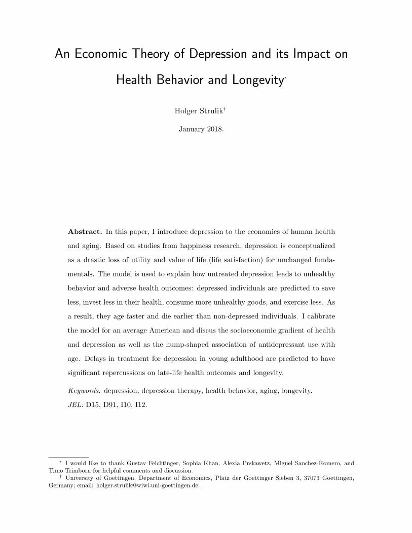
with the life cycle choices of the non-depressed benchmark American, which are shown in Figure

1 by blue (solid) lines. With advancing age, the individual develops more health deficits, spends

more on health, consumes less unhealthy goods, and exercises less. At age 75.5, the individual

dies when the terminal condition for health deficits D is reached. The life-cycle choices of non-

depressed individuals are discussed in detail by Dalgaard and Strulik (2014) and Schuenemann

et al. (2017a). The new choice variable here is physical exercise, which declines with age since

exercise becomes increasingly painful as the individual develops more health deficits.

The life-cycle choices of the depressed individual are shown by red (dashed) lines in Figure 1.

The relative change of behavior and age at death, compared to the non-depressed benchmark

14

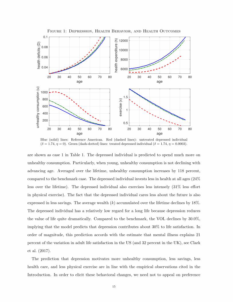
Figure 1: Depression, Health Behavior, and Health Outcomes

20 30 40 50 60 70 80

age

0.04

0.06

0.08

0.1health d

eficits (

D)

20 30 40 50 60 70 80

age

6000

8000

10000

12000

health e

xpenditure

(h)

20 30 40 50 60 70 80

age

200

400

600

800

1000

unhealthy c

onsum

ption (

u)

20 30 40 50 60 70 80

age

0.5

1

1.5

exerc

ise (

x)

Blue (solid) lines: Reference American. Red (dashed lines): untreated depressed individual(δ = 1.74, η = 0). Green (dash-dotted) lines: treated depressed individual (δ = 1.74, η = 0.0003).

are shown as case 1 in Table 1. The depressed individual is predicted to spend much more on

unhealthy consumption. Particularly, when young, unhealthy consumption is not declining with

advancing age. Averaged over the lifetime, unhealthy consumption increases by 118 percent,

compared to the benchmark case. The depressed individual invests less in health at all ages (24%

less over the lifetime). The depressed individual also exercises less intensely (31% less effort

in physical exercise). The fact that the depressed individual cares less about the future is also

expressed in less savings. The average wealth (k) accumulated over the lifetime declines by 18%.

The depressed individual has a relatively low regard for a long life because depression reduces

the value of life quite dramatically. Compared to the benchmark, the VOL declines by 30.0%,

implying that the model predicts that depression contributes about 30% to life satisfaction. In

order of magnitude, this prediction accords with the estimate that mental illness explains 21

percent of the variation in adult life satisfaction in the US (and 32 percent in the UK), see Clark

et al. (2017).

The prediction that depression motivates more unhealthy consumption, less savings, less

health care, and less physical exercise are in line with the empirical observations cited in the

Introduction. In order to elicit these behavioral changes, we need not to appeal on preference

15

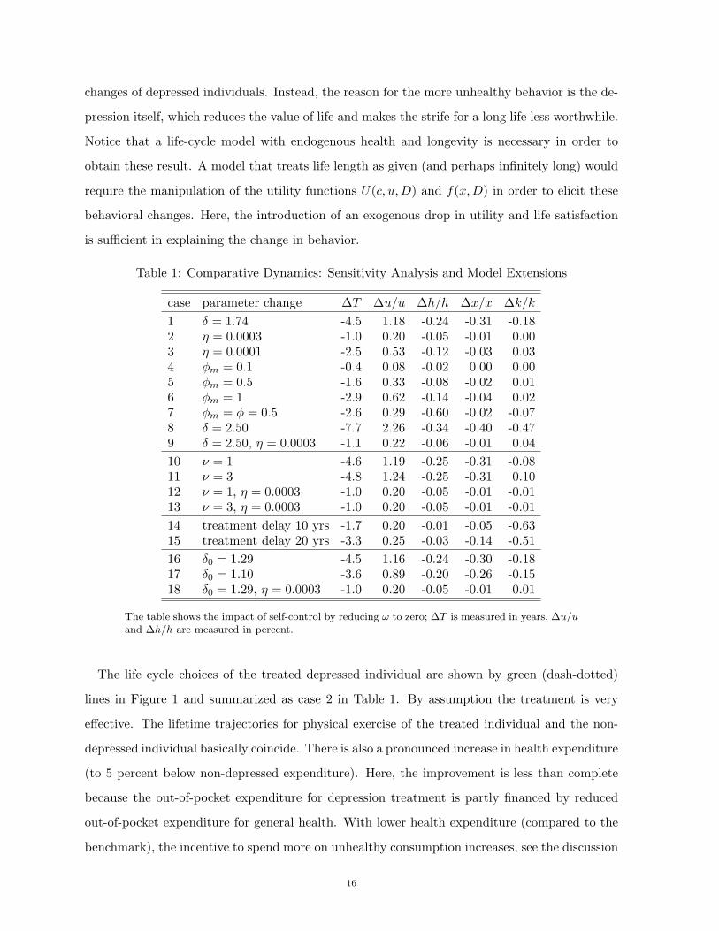
changes of depressed individuals. Instead, the reason for the more unhealthy behavior is the de-

pression itself, which reduces the value of life and makes the strife for a long life less worthwhile.

Notice that a life-cycle model with endogenous health and longevity is necessary in order to

obtain these result. A model that treats life length as given (and perhaps infinitely long) would

require the manipulation of the utility functions U(c, u,D) and f(x,D) in order to elicit these

behavioral changes. Here, the introduction of an exogenous drop in utility and life satisfaction

is sufficient in explaining the change in behavior.

Table 1: Comparative Dynamics: Sensitivity Analysis and Model Extensions

case parameter change ∆T ∆u/u ∆h/h ∆x/x ∆k/k

1 δ = 1.74 -4.5 1.18 -0.24 -0.31 -0.182 η = 0.0003 -1.0 0.20 -0.05 -0.01 0.003 η = 0.0001 -2.5 0.53 -0.12 -0.03 0.034 φm = 0.1 -0.4 0.08 -0.02 0.00 0.005 φm = 0.5 -1.6 0.33 -0.08 -0.02 0.016 φm = 1 -2.9 0.62 -0.14 -0.04 0.027 φm = φ = 0.5 -2.6 0.29 -0.60 -0.02 -0.078 δ = 2.50 -7.7 2.26 -0.34 -0.40 -0.479 δ = 2.50, η = 0.0003 -1.1 0.22 -0.06 -0.01 0.04

10 ν = 1 -4.6 1.19 -0.25 -0.31 -0.0811 ν = 3 -4.8 1.24 -0.25 -0.31 0.1012 ν = 1, η = 0.0003 -1.0 0.20 -0.05 -0.01 -0.0113 ν = 3, η = 0.0003 -1.0 0.20 -0.05 -0.01 -0.01

14 treatment delay 10 yrs -1.7 0.20 -0.01 -0.05 -0.6315 treatment delay 20 yrs -3.3 0.25 -0.03 -0.14 -0.51

16 δ0 = 1.29 -4.5 1.16 -0.24 -0.30 -0.1817 δ0 = 1.10 -3.6 0.89 -0.20 -0.26 -0.1518 δ0 = 1.29, η = 0.0003 -1.0 0.20 -0.05 -0.01 0.01

The table shows the impact of self-control by reducing ω to zero; ∆T is measured in years, ∆u/uand ∆h/h are measured in percent.

The life cycle choices of the treated depressed individual are shown by green (dash-dotted)

lines in Figure 1 and summarized as case 2 in Table 1. By assumption the treatment is very

effective. The lifetime trajectories for physical exercise of the treated individual and the non-

depressed individual basically coincide. There is also a pronounced increase in health expenditure

(to 5 percent below non-depressed expenditure). Here, the improvement is less than complete

because the out-of-pocket expenditure for depression treatment is partly financed by reduced

out-of-pocket expenditure for general health. With lower health expenditure (compared to the

benchmark), the incentive to spend more on unhealthy consumption increases, see the discussion

16

of equation (14). The treatment almost eliminates the entire impact of depression on happiness.

The value of life of the treated individual is 1% below the benchmark (compared to 30% of the

non-treated). As a result, aggregate savings are now even higher than for the non-depressed

individual. The treatment cured the low valuation of a long life and raised the need for savings

to finance the out-of-pocket share of mental health care in old age.

Case 3 in Table 1 considers outcomes when depression treatment is less effective (η declines

to 0.0001). As a result, treatment is not able to sufficiently restore the value of life. Depressed

individuals still exhibit less healthy behavior than the non-depressed, and treatment saves only

2 years of longevity (T is reduced by 2.5 years instead of 4.5 when untreated).

Case 4 to 6 consider different out-of-pocket shares for depression treatment. A larger out-

of-pocket share reduces the budget that remains for other expenditures. In particular, general

health investment declines with increasing out-of-pocket share for depression treatment. This

increases the marginal productivity of health care and induces more unhealthy consumption

(see (14)). Physical exercise, in contrast, is almost restored to the non-depressed level. This

indicates that depression is still (almost) cured, as in case 3. The difference in health deficit

accumulation and age of death between these cases operates through the budget constraint.

This can also be seen in the response of savings. A higher out-of-pocket share induces more

savings for depression treatment in old age, which, among other things, leaves less income to be

spent on current health investments. For completeness, case 7 considers a simultaneous increase

in the out-of-pocket share for both types of health expenditure. As expected, this paricularly

harms investments in general health care.

Case 8 considers a more severe depression: δ increases to 2.5, which means that, untreated,

depression can be attributed to the loss of 7.7 years of lifetime. Interestingly, when treated, the

health outcomes and behavioral changes are almost the same as in the case of milder depression,

as the comparison between cases 9 and 2 shows. The biggest difference is in terms of savings

since more severe forms of depression require more expenditure for treatment in old age.

5. Applications and Extensions

5.1. Depression and Labor Supply. So far, we have ignored the additional indirect effects

of depression on life-cycle outcomes through reduced productivity and labor income. The recent

study of Peng et al. (2016) suggests that the effects on income may indeed be small. Depression

17

is estimated to reduce the probability of employment by 2.6 percentage points and to increase

annual work loss days by 1.4 days. Earlier studies suggested higher effects on labor market

outcomes (e.g. Chatterji et al., 2011). In the model, a convenient way to acknowledge labor

market effects is through early retirement. Subsequently, we assume that the previous age of

retirement (R = 65) is reduced to R−νδemη. In cases 10 and 11 of Table 1, we consider relatively

strong effects of depression on retirement and lifetime income by setting ν = 1 and ν = 3. This

means that, in case 10, the individual receives 1.74 times (1-0.45) times w, i.e. $ 33,800 less

lifetime income. In case 11, it implies that depression reduces lifetime income by $ 101,400.

Comparing results of case 10 and 11 with case 1 shows that outcomes for untreated depression

are, perhaps surprisingly, only marginally affected by the income feedback although the impact

on income is large. In other words, the direct depression effect on life satisfaction is much stronger

than any indirect effect through income, as suggested in related empirical studies (Layard et al.

2013). Health behavior, in turn, responds more sensitively to depression than to income. Case

12 and 13 further confirm this assessment by showing that the treatment outcomes in case of

feedback effects also deviate only insignificantly from the benchmark treatment (Case 2).

5.2. Delayed Treatment. As discussed in the Introduction, a large share of depression cases

remains untreated. One reason for a delay in treatment could be that individuals and their

relatives fail to self-diagnose the disease and confound and perhaps rationalize it as (justified)

sadness “with a reason”. In Table 1, case 14, we see the health outcomes when depression is

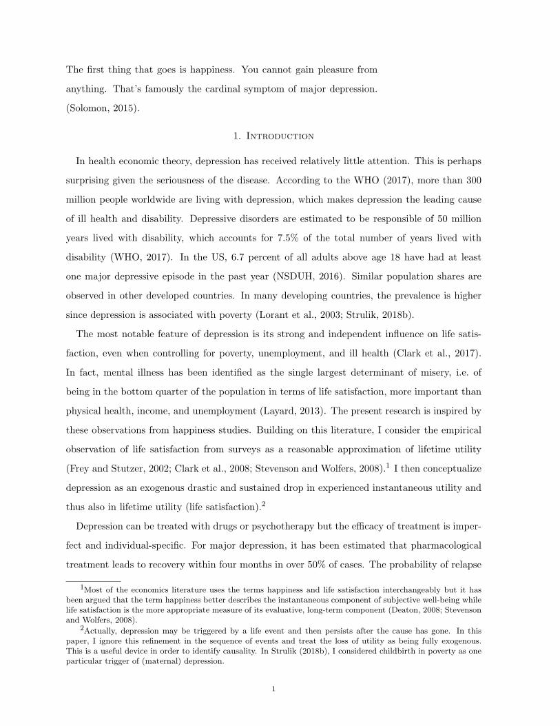
treated with a delay of 10 years. The individual loses 1.7 years of lifetime, compared to 1.0 year

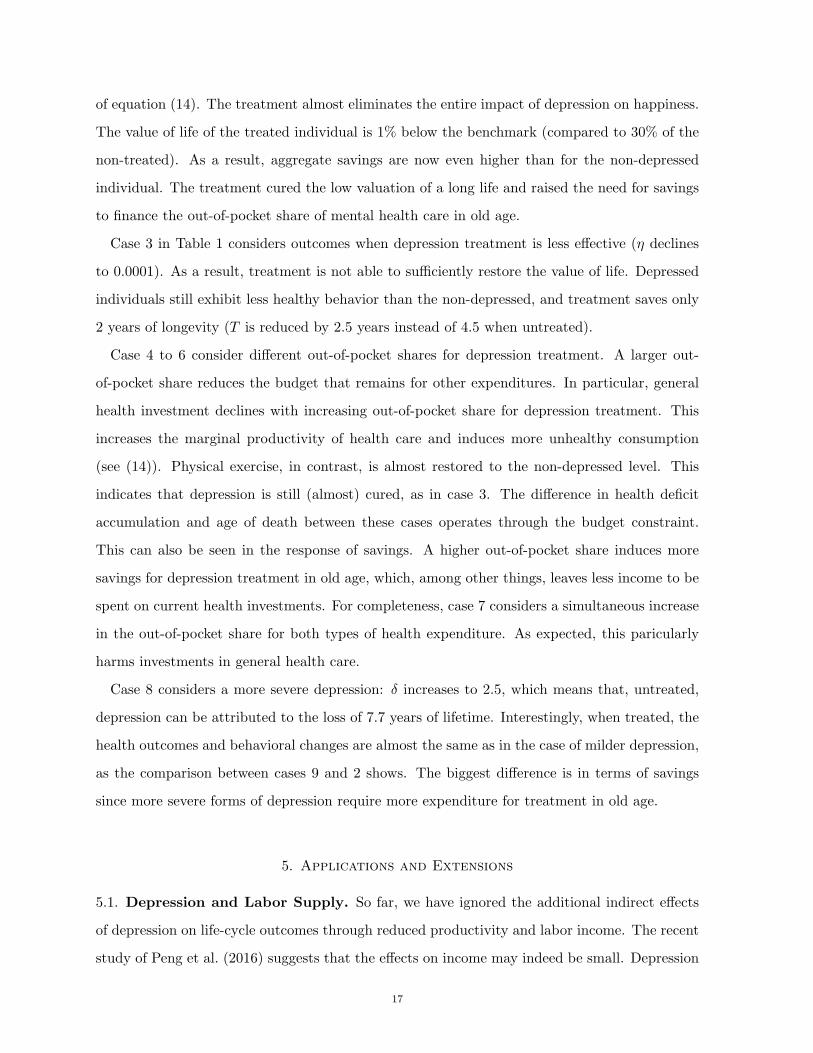
if depression is treated immediately. The life-cycle behavior shown in Figure 2 explains why.

Blue (solid) lines reiterate the life-cycle trajectories of the benchmark non-depressed individual.

Red (dashed) lines show the trajectories when treatment is delayed by 10 years. They coincide

with those of the untreated individual from Figure 1 until treatment sets in. Then, the treated

depressed individual actually behaves in a more healthy manner than the non-depressed indi-

vidual: he invests more in health, consumes less unhealthy goods, and engages in somewhat

more physical exercise. But it is too late to fully compensate for the faster deteriorating health

during early adulthood. Health deficits continue to accumulate faster after treatment and lead

to an earlier death.

Case 15 in Table 1 and the green (dash-dotted) trajectories in Figure 2 show the outcome when

treatment is delayed by 20 years. The reduction of longevity now more than triples compared

18

Figure 2: Delayed Treatment

20 30 40 50 60 70 80

age

0.04

0.06

0.08

0.1health d

eficits (

D)

20 30 40 50 60 70 80

age

6000

8000

10000

12000

health e

xpenditure

(h)

20 30 40 50 60 70 80

age

200

400

600

800

1000

unhealthy c

onsum

ption (

u)

20 30 40 50 60 70 80

age

0.8

1

1.2

1.4

1.6

1.8

exerc

ise (

x)

Blue (solid lines): non-depressed individual. Red (dashed lines): benchmark depressed individualwith treatment delay of 10 years. Green (dashed-dotted lines): benchmark depressed individualwith treatment delay of 20 years.

to benchmark treatment (case 2). Aggregate behavioral outcomes are in fact more similar to

completely untreated depression than to instantly treated depression. Significantly increased

health expenditure after treatment and reduced unhealthy consumption fail to compensate for

the lost health during the depression phase. These outcomes are a manifestation of the quasi-

exponential nature of the health deficit accumulation, which leads to the amplification of early-

life health shocks over time. The health capital model (Grossman, 1972), in contrast, would

predict that initial differences in health shocks – or, in the current case, the consequences of

delayed treatment – depreciate as the individual ages (see Almond and Currie, 2011 and Dalgaard

et al., 2017 for a critique). The health deficit model, in contrast, captures the cumulative

character of health deficit accumulation emphasized in gerontology (e.g. Arking, 2006). The

damage done in young adulthood by unhealthy consumption, little health investment, and little

physical exercise is never fully repaired after the onset of depression treatment. These outcomes

highlight the importance of diagnosing and treating the disease early.

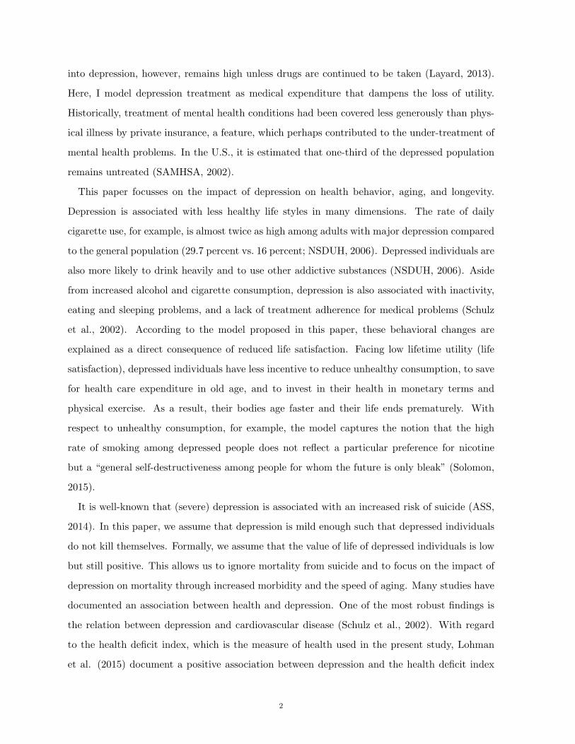
5.3. Income Gradient. We next look at the income gradients of longevity and the value of

life and how they are transformed by depression. To do so, we feed different values of labor

19

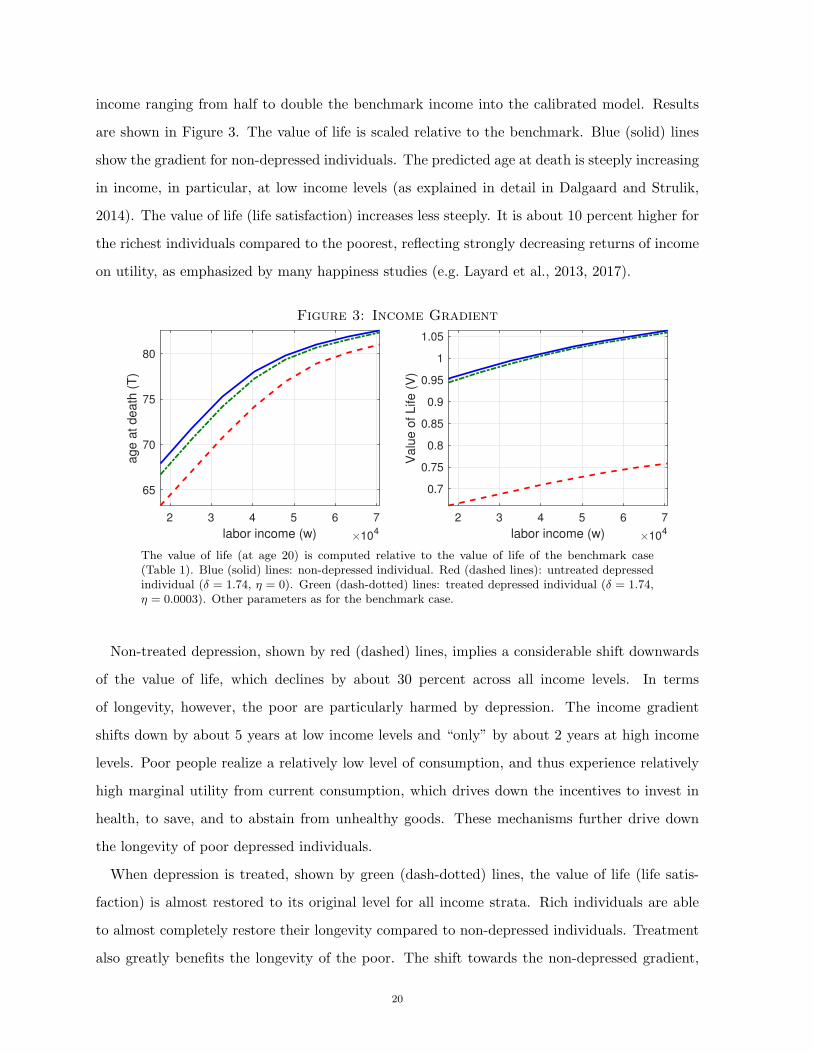
income ranging from half to double the benchmark income into the calibrated model. Results

are shown in Figure 3. The value of life is scaled relative to the benchmark. Blue (solid) lines

show the gradient for non-depressed individuals. The predicted age at death is steeply increasing

in income, in particular, at low income levels (as explained in detail in Dalgaard and Strulik,

2014). The value of life (life satisfaction) increases less steeply. It is about 10 percent higher for

the richest individuals compared to the poorest, reflecting strongly decreasing returns of income

on utility, as emphasized by many happiness studies (e.g. Layard et al., 2013, 2017).

Figure 3: Income Gradient

2 3 4 5 6 7

labor income (w) 104

65

70

75

80

age a

t death

(T

)

2 3 4 5 6 7

labor income (w) 104

0.7

0.75

0.8

0.85

0.9

0.95

1

1.05

Valu

e o

f Life (

V)

The value of life (at age 20) is computed relative to the value of life of the benchmark case(Table 1). Blue (solid) lines: non-depressed individual. Red (dashed lines): untreated depressedindividual (δ = 1.74, η = 0). Green (dash-dotted) lines: treated depressed individual (δ = 1.74,η = 0.0003). Other parameters as for the benchmark case.

Non-treated depression, shown by red (dashed) lines, implies a considerable shift downwards

of the value of life, which declines by about 30 percent across all income levels. In terms

of longevity, however, the poor are particularly harmed by depression. The income gradient

shifts down by about 5 years at low income levels and “only” by about 2 years at high income

levels. Poor people realize a relatively low level of consumption, and thus experience relatively

high marginal utility from current consumption, which drives down the incentives to invest in

health, to save, and to abstain from unhealthy goods. These mechanisms further drive down

the longevity of poor depressed individuals.

When depression is treated, shown by green (dash-dotted) lines, the value of life (life satis-

faction) is almost restored to its original level for all income strata. Rich individuals are able

to almost completely restore their longevity compared to non-depressed individuals. Treatment

also greatly benefits the longevity of the poor. The shift towards the non-depressed gradient,

20

however, is incomplete. Treatment costs matter more for the poor and drive down investment

in general health and savings (for health expenditure in old age).

Figure 4: Income Gradient (φm = 1)

2 3 4 5 6 7

labor income (w) 104

65

70

75

80

age a

t death

(T

)

2 3 4 5 6 7

labor income (w) 104

0.7

0.75

0.8

0.85

0.9

0.95

1

1.05

Valu

e o

f Life (

V)

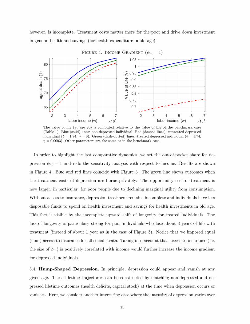
The value of life (at age 20) is computed relative to the value of life of the benchmark case(Table 1). Blue (solid) lines: non-depressed individual. Red (dashed lines): untreated depressedindividual (δ = 1.74, η = 0). Green (dash-dotted) lines: treated depressed individual (δ = 1.74,η = 0.0003). Other parameters are the same as in the benchmark case.

In order to highlight the last comparative dynamics, we set the out-of-pocket share for de-

pression φm = 1 and redo the sensitivity analysis with respect to income. Results are shown

in Figure 4. Blue and red lines coincide with Figure 3. The green line shows outcomes when

the treatment costs of depression are borne privately. The opportunity cost of treatment is

now larger, in particular ,for poor people due to declining marginal utility from consumption.

Without access to insurance, depression treatment remains incomplete and individuals have less

disposable funds to spend on health investment and savings for health investments in old age.

This fact is visible by the incomplete upward shift of longevity for treated individuals. The

loss of longevity is particulary strong for poor individuals who lose about 3 years of life with

treatment (instead of about 1 year as in the case of Figure 3). Notice that we imposed equal

(non-) access to insurance for all social strata. Taking into account that access to insurance (i.e.

the size of φm) is positively correlated with income would further increase the income gradient

for depressed individuals.

5.4. Hump-Shaped Depression. In principle, depression could appear and vanish at any

given age. These lifetime trajectories can be constructed by matching non-depressed and de-

pressed lifetime outcomes (health deficits, capital stock) at the time when depression occurs or

vanishes. Here, we consider another interesting case where the intensity of depression varies over

21

the lifetime (and may only at its peak, be experienced as unbearable). This scenario relates to

Blanchflower and Oswald (2008, 2016), who argue that life satisfaction is u-shaped across the

life cycle and that this pattern is partly explained by an invertedly u-shaped age pattern of the

prevalence or intensity of depression. As corroborating evidence, they show that the prevalence

of antidepressant use is invertedly u-shaped in age with a peak in the late forties.

In order to conveniently represent these ideas we replace the constant δ with a depression

function for age t:

δ(t) = max{

0, δ0 exp(ψ1t− ψ2t2)− ξ

}

. (19)

The ψ-parameters control the age pattern, δ0 controls the severity of depression, and ξ is a

perception threshold. With ξ, we can determine at which ages depression is perceived as salient

such that it motivates a desire for treatment. To begin with, we set ξ = 0 and adjust the other

parameters such that depression reaches a maximum at age 49 and that, if untreated, leads to

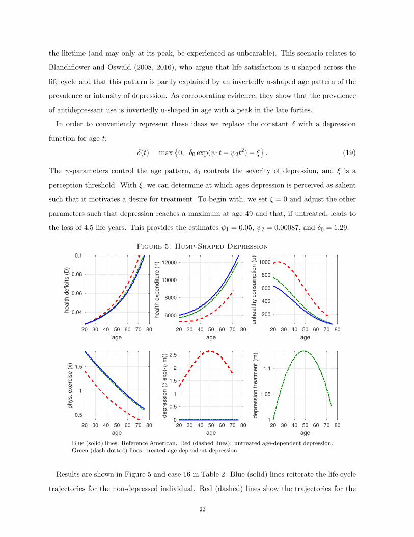
the loss of 4.5 life years. This provides the estimates ψ1 = 0.05, ψ2 = 0.00087, and δ0 = 1.29.

Figure 5: Hump-Shaped Depression

20 30 40 50 60 70 80

age

0.04

0.06

0.08

0.1

he

alth

de

ficits (

D)

20 30 40 50 60 70 80

age

6000

8000

10000

12000

he

alth

exp

en

ditu

re (

h)

20 30 40 50 60 70 80

age

200

400

600

800

1000

un

he

alth

y c

on

su

mp

tio

n (

u)

20 30 40 50 60 70 80

age

0.5

1

1.5

ph

ys.

exe

rcis

e (

x)

20 30 40 50 60 70 80

age

0

0.5

1

1.5

2

2.5

de

pre

ssio

n (

exp

(- m

))

20 30 40 50 60 70 80

age

1

1.05

1.1

de

pre

ssio

n t

rea

tme

nt

(m)

Blue (solid) lines: Reference American. Red (dashed lines): untreated age-dependent depression.Green (dash-dotted) lines: treated age-dependent depression.

Results are shown in Figure 5 and case 16 in Table 2. Blue (solid) lines reiterate the life cycle

trajectories for the non-depressed individual. Red (dashed) lines show the trajectories for the

22

non-treated individual. Unsurprisingly, the results for health behavior and outcomes look very

similar to those for the benchmark case from Figure 1. Depression, shown at the center panel

at the bottom of Figure 3, is (by design) invertedly u-shaped in its intensity. Remarkably, the

impact of depression on the value of life (life satisfaction) is higher than for the benchmark run.

The VOL declines by 34.2 % instead of 30.0%. The reason is that for young individuals (whose

instantaneous utility is not much discounted to the present) depression is on the rise while for

old individuals (whose instantaneous utility is heavily discounted to the present) depression

declines.

Alternatively, we could match the impact of depression on the value of life to be equal to the

benchmark depression case (i.e. 30%). This leads to the estimate δ = 1.10. Results are shown as

case 17 in Table 2. The impact on health outcomes is now smaller because depression in young

age has a particularly severe impact on health outcomes through reduced health investments

and increased unhealthy behavior and the caused cumulative damage. Finally, case 18 in Table

1 shows that health outcomes for treated u-shaped depression do not differ significantly from

those for constant depression (case 2).

We next explore sensitivity with respect to ξ, the threshold of depression perception. Keeping

the other parameter values as specified above, a value of ξ = 1.3 implies that (perceptible)

depression sets in shortly after the 20th birthday (at model age t = 0.02) and then gradually

rises in severity until age 49 after which it declines again to a low positive value before death.

A value of 2.6 implies that depression is perceived only as a “midlife low” between ages 45 and

53.

Figure 6: Share of Population Using Anti-Depressants

20 30 40 50 60 70 80

age

0

0.02

0.04

0.06

0.08

0.1

0.12

pop. share

usin

g a

ntidre

ssants

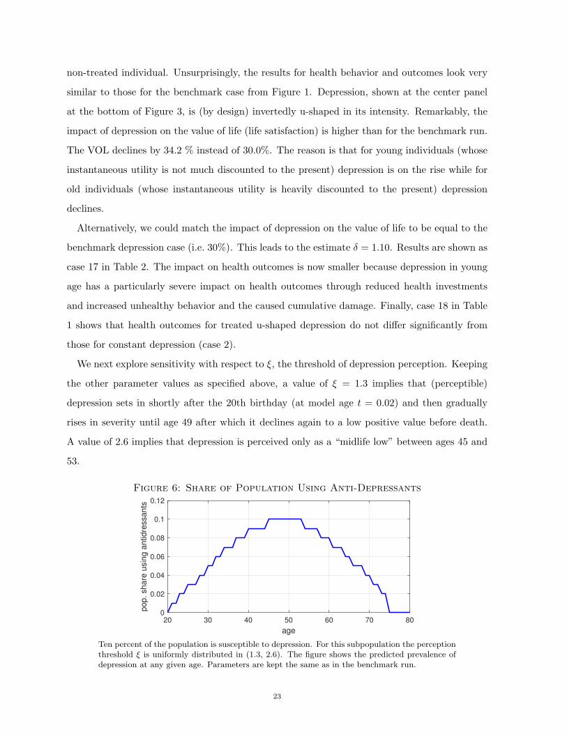
Ten percent of the population is susceptible to depression. For this subpopulation the perceptionthreshold ξ is uniformly distributed in (1.3, 2.6). The figure shows the predicted prevalence ofdepression at any given age. Parameters are kept the same as in the benchmark run.

23

Suppose that 10 percent of the population are susceptible to depression and that among

these individuals ξ is uniformly distributed in (1.3, 2.6). In order to make inferences about the

association of age and aggregate demand for antidepressants, we run the model (with otherwise

benchmark parameters) for 10 equally-spaced draws from (1.3, 2.6) and compute for any age

(in the discrete space of natural numbers) whether antidepressants are used. Figure 6 shows

the predicted population share using antidepressants. The inverted u replicates the empirical

association between age and antidepressant use estimated by Blanchflower and Oswald (2015).

6. Conclusion

This paper introduces depression into health economic theory and evaluates its impact on

life-cycle health behavior and longevity. Inspired by happiness research, depression has been

conceptualized as a potentially large drop in utility (happiness) and the value of life (life satis-

faction). Successful therapy (partly) restores original utility and life satisfaction. These elements

have been integrated into a life-cycle model of health deficit accumulation, augmented by utility-

enhancing unhealthy consumption and utility-reducing but health-enhancing physical exercise.

The model explains why depressed people consume more unhealthy goods, save less, invest

less in their health, and exert less effort in physical exercise. These responses are elicited without

transforming the utility function for consumption and exercise. They are an expression of the

depression itself in a model that considers longevity as endogenous and at least partly malleable

by health behavior. Since depressed people experience less life satisfaction, they strive less to

extend life and are less motivated to exhibit healthy behavior.

The model has been calibrated to predict the life-cycle trajectories of health behavior and

health outcomes for a non-depressed Reference American. Introducing depression as a 30% drop

in life satisfaction rationalizes changes in health behavior that reduce the length of life by about 4

years. Extensions of the model have shown that these results are obtained largely independently

from the size of (reasonable) feedback effects of depression on labor supply and lifetime income.

The timing of treatment, however, is predicted to be crucial. Delays in diagnosis or treatment

lead to severe losses in health that are not fully recovered in the treatment period. The reason

is that the (gerontologically founded) health deficit model amplifies the late-life consequences of

health shocks in early life. In the present context, this means that individuals do not manage

24

to compensate fully for the health destroyed by unhealthy behavior during untreated depression

in early adulthood.

Since this study is a first attempt to discuss depression in the context of health and longevity,

there are ample possibilities to further extend and refine the theory. For example, it could

also be taken into account that depression has a direct biological impact on health through, for

example, blood pressure, inflammation, or immune function. Another possibility is to analyze

inferior and potentially health-damaging self-treatment of depression symptoms, for example, by

excessive alcohol consumption. This could be a particularly interesting endeavor in the context

of the income gradient of longevity and limited access to insurance-covering clinical depression

treatment. Such an analysis could also consider the addictive potential of the applied self-

treatment, investigate the repercussions of unhealthy addiction on longevity (Strulik, 2017),

and explain the positive association between depression and addiction (Solomon, 2015).

The assumed exogeneity of depression is a reasonable first approximation of reality and a

useful device in order to identify causality. An extension, however, could discuss depression

triggered by bad health and investigate the interdependence of both phenomena. In particular,

chronic pain seems to be associated with depression (DePaulo and Horvitz, 2002). This fact

could establish a link between depression, use of antidepressants and painkiller consumption,

and contribute to the literature on the opioid epidemic .

25

Appendix

6.1. Derivation of (14) to (18). We first write the first order conditions (5)–(9) and the

costate equations (11)–(12) for the parameterized utility function.

(

D

D0

)

−ǫ

[θc+ (1− θ)u]−σ θ = λk (A.1)

(

D

D0

)

−ǫ

[θc+ (1− θ)u]−σ (1− θ) ≤ λkq − λDµBωuω−1 with = for u > 0 (A.2)

− λDµγAγ−1 = λkφp (A.3)

− λDµκExκ−1 = τ

(

D

D0

)χ

(A.4)

− δηe−ηm≤ λkφmpm with = for m > 0. (A.5)

λr = λkρ− λk (A.6)

− ǫ

(

D

D0

)

−ǫ−1 [θc+ (1− θ)u]1−σ− 1

1− σ− χ

(

D

D0

)χ−1

τx+ µλD = λDρλD (A.7)

Let c ≡ θc+(1− θ)u define a weighted measure of total consumption. From (A.1) and (A.2) we

obtain1− θ

θλk − qλk + λDµBωu

ω−1≤ 0.

Using (A.3) to eliminate λD and and dividing by λk we obtain

1− θ

θ− q ≤

φp

γAhγ−1Bωuω−1.

Solving for u provides (14) in the text. Inserting (A.3) into (A.4) provides:

λkφp

γAhγ−1κExκ−1 =

(

D

D0

)χ

τ.

Inserting λk from (A.1) we get

(

D

D0

)

−(ǫ+χ) φp

γAhγ−1θc−σκE = τx1−κ.

Solving for x provides (15) in the text. Inserting (A.1) into (A.5) we obtain

δη(cσ(D/D0)ǫ

φmpm≤ eηm.

Solving for m provides (16) in the text. Log-differentiating (A.1) provides

−ǫD

D− σ

˙c

c=λkλk.

Eliminating λk/λk using (A.6) provides (17) in the text. Log-differentiating (A.3) and eliminat-

ing λk/λk using (A.6) provides

h

h=

1

1− γ

(

ρ− r −λDλD

)

. (A.8)

26

Using (A.3), equation (A.7) can be written as

−λDλD

= µ− ρ−

[

ǫ

(

D

D0

)

−ǫ−1 c1−σ − 1

1− σ+ χ

(

D

D0

)χ−1

τx

]

µγAhγ−1

λkφp.

Using (A.1) this can be expressed as

−λDλD

= µ− ρ−

[

ǫc1−σ − 1

1− σ+ χ

(

D

D0

)χ+ǫ

τx

]

µγAhγ−1cσ

λkφpD. (A.9)

Inserting (A.9) into (A.8) provides (18) in the text.

27

References

Almeida, O. P., Alfonso, H., Hankey, G. J., and Flicker, L. (2010). Depression, antidepressant

use and mortality in later life: the Health In Men Study. PLoS One, 5(6), e11266.

Almond, D., and Currie, J. (2011). Killing me softly: The fetal origins hypothesis. Journal of

Economic Perspectives 25(3), 153-72.

ASS (2014). Depression and suicide risk. American Association of Suicidology, http://www.

suicidology.org/resources/facts-statistics

Beck, A.T. (1967). Depression: Causes and Treatment. Philadelphia: University of Pennsylva-

nia Press.

Blanchflower, D.G., and Oswald, A.J. (2008). Is well-being U-shaped over the life cycle? Social

Science and Medicine 66(8), 1733-1749.

Blanchflower, D.G., and Oswald, A. J. (2016). Antidepressants and age: A new form of evidence

for U-shaped well-being through life. Journal of Economic Behavior and Organization 127,

46-58.

BLS (2002). Consumer Expenditures in 2000, United States Department of Labor, Bureau of

Labor Statistics, Report 958.

BLS (2011). State average annual pay for 2000 and 2001, United States Department of Labor,

Bureau of Labor Statistics (http://www.bls.gov/news.release/annpay.t01.htm).

Case, A., and Deaton, A. (2017). Mortality and morbidity in the 21st century. Brookings Papers

on Economic Activity Spring 2017, 397-476.

Chatterji, P., Alegria, M., and Takeuchi, D. (2011). Psychiatric disorders and labor market

outcomes: Evidence from the National Comorbidity Survey-Replication. Journal of Health

Economics 30(5), 858-868.

Clark, A.E., P. Frijters, and M.A. Shields, 2008, Relative income, happiness, and utility: An

explanation for the Easterlin paradox and other puzzles, Journal of Economic Literature 46,

95-144.

Clark, A.E., Fleche, S., Layard, R., Powdthavee, N., and Ward, G. (2017). The key determinants

of happiness and misery.. In: Helliwell, J., Layard, R., and Sachs, J. (eds.) World Happiness

Report 2017, New York: Sustainable Development Solutions Network, United Nations.

Dalgaard, C-J., and Strulik, H. (2014). Optimal aging and death: Understanding the Preston

Curve, Journal of the European Economic Association 12, 672-701.

Dalgaard, C-J. and Strulik, H. (2017). The genesis of the golden age: Accounting for the rise in

health and leisure. Review of Economic Dynamics, 24, 32-151.

Dalgaard, C-J., Hansen, C.W., and Strulik, H. (2017). Accounting for Fetal Origins: Health

Capital vs. Health Deficits, Discussion Paper, University of Copenhagen.

28

Darden, M., Gilleskie, D.B., and Strumpf, K. (2015). Smoking and Mortality: New Evidence

from a Long Panel, Discussion Paper.

Deaton, A., 2008, Income, Health, and Well-Being around the World: Evidence from the Gallup

World Poll, Journal of Economic Perspectives 22(2), 53-72.

De Neve, J-E., Diener, E., Tay, L., and Xuereb, C. (2013). The objective benefits of subjective

well-being. In J. F. Helliwell, R. Layard, and J. Sachs (Eds.), World happiness report 2013.

Volume 2. (pp. 54-79). New York: UN Sustainable Network Development Solutions Network.

DePaulo Jr, J.R., and Horvitz, L. A. (2002). Understanding depression: What we know and

what you can do about it. John Wiley & Sons, Hoboken, New Jersey.

De Quidt, J., and Haushofer, J. (2016). Depression for economists. National Bureau of Economic

Research Working Paper w22973.

Dolan, P., Lee, H., and Peasgood, T. (2012). Losing Sight of the Wood for the Trees. Pharma-

coeconomics 30(11), 1035-1049.

Finkelstein, A., Luttmer, E.F., and Notowidigdo, M.J. (2013). What good is wealth without

health? The effect of health on the marginal utility of consumption. Journal of the European

Economic Association 11(1), 221-258.

Fleche, S., and Layard, R. (2017). Do more of those in misery suffer from poverty, unemployment

or mental illness? Kyklos 70(1), 27-41.

Frey, B.S. and A. Stutzer, 2002, What can economists learn from happiness research?, Journal

of Economic Literature 40, 402-435.

Gallo, J.J., Bogner, H.R., Morales, K.H., Post, E.P., Lin, J.Y., and Bruce, M.L. (2007). The

Effect of a Primary Care PracticeBased Depression Intervention on Mortality in Older Adults.

Annals of internal medicine, 146(10), 689-698.

Goesling, J., Henry, M.J., Moser, S.E., Rastogi, M., Hassett, A.L., Clauw, D.J., and Brummett,

C.M. (2015). Symptoms of depression are associated with opioid use regardless of pain severity

and physical functioning among treatment-seeking patients with chronic pain. The Journal

of Pain 16(9), 844-851.

Grossman, M. (1972). On the concept of health capital and the demand for health. Journal of

Political Economy 80, 223-255.

Gusmao, R., Quintao, S., McDaid, D., Arensman, E., Van Audenhove, C., Coffey, C., ... and

Hegerl, U. (2013). Antidepressant utilization and suicide in Europe: an ecological multi-

national study. PLoS One 8(6), e66455.

Guven, C. (2012). Reversing the question: Does happiness affect consumption and savings

behavior?. Journal of Economic Psychology 33(4), 701-717.

29

Holford, T.R., Levy, D.T., McKay, L.A., Clarke, L., Racine, B., Meza, R., ... and Feuer, E.J.

(2014). Patterns of birth cohortspecific smoking histories, 1965–2009. American Journal of

Preventive Medicine 46(2), e31-e37.

Jha, P., Ramasundarahettige, C., Landsman, V., Rostron, B., Thun, M., Anderson, R. N., ...

and Peto, R. (2013). 21st-century hazards of smoking and benefits of cessation in the United

States. New England Journal of Medicine 368(4), 341-350.

Katolik, A., and Oswald, A.J. (2017). Antidepressants for Economists and Business-School

Researchers: An Introduction and Review. Discussion Paper, University of Warwick.

Kessler, R. C., Aguilar-Gaxiola, S., Alonso, J., Chatterji, S., Lee, S., Ormel, J., ... and Wang,

P. S. (2009). The global burden of mental disorders: an update from the WHO World Mental

Health (WMH) surveys. Epidemiology and Psychiatric Sciences 18(1), 23-33.

Layard, R., Chisholm, D., Patel, V., and Saxena, S. (2013). Mental illness and unhappiness.

In: Helliwell, J., Layard, R., and Sachs, J. (eds.) World Happiness Report 2013, New York:

Sustainable Development Solutions Network, United Nations.

Linden, W., Stossel, C., and Maurice, J. (1996). Psychosocial interventions for patients with

coronary artery disease: a meta-analysis. Archives of Internal Medicine 156(7), 745-752.

Lohman, M., Dumenci, L., and Mezuk, B. (2015). Depression and frailty in late life: evidence

for a common vulnerability. Journals of Gerontology Series B 71(4), 630-640.

Ludwig, J., Marcotte, D.E., and Norberg, K. (2009). Anti-depressants and suicide. Journal of

Health Economics 28(3), 659-676.

Machlin, S. and Carper, K. (2014), Out-of-Pocket Health Care Expenses by Age and Insurance

Coverage. Statistical Brief 441, Agency for Healthcare Research and Quality, Rockville, MD.

Mezuk, B., Edwards, L., Lohman, M., Choi, M., and Lapane, K. (2012). Depression and frailty

in later life: a synthetic review. International Journal of Geriatric Psychiatry 27(9), 879-892.

Mitnitski, A.B., Mogilner, A.J., MacKnight, C., and Rockwood, K. (2002a). The accumulation

of deficits with age and possible invariants of aging. Scientific World 2, 1816-1822.

Mitnitski, A.B., Mogilner, A.J., MacKnight, C., and Rockwood, K. (2002b). The mortality rate

as a function of accumulated deficits in a frailty index. Mechanisms of ageing and development

123, 1457-1460.

Mitnitski, A., Song, X., Skoog, I., Broe, G.A., Cox, J.L., Grunfeld, E., and Rockwood, K.,

2005. Relative fitness and frailty of elderly men and women in developed countries and their

relationship with mortality. Journal of the American Geriatrics Society 53, 2184–2189.

Murphy, K.M. and Topel, R.H., 2006, The value of health and longevity, Journal of Political

Economy 114, 871–904.

30

NSDUH (2006). Results from the 2006 National Survey on Drug Use and Health: National

Findings, Substance Abuse and Mental Health Services Administration, NSDUH Series H-32,

DHHS Publication No. SMA 07-4293). Rockville, MD.

NSDUH (2016). Key substance use and mental health indicators in the United States: Results

from the 2016 National Survey on Drug Use and Health. HHS Publication No. SMA 17-5044,

NSDUH Series H-52). Rockville, MD.

NVSS (2012). National Vital Statistics Report 61(3), US Department of Health and Human

Services, National Vital Statistics System.

OECD (2016), Gross pension replacement rates. OECD Data (https://data.oecd.org/pension/

gross-pension-replacement-rates.htm

Lorant, V., Delige, D., Eaton, W., Robert, A., Philippot, P., and Ansseau, M. (2003). Socioeco-

nomic inequalities in depression: a meta-analysis. American Journal of Epidemiology 157(2),

98-112.

Paykel, E. S. (2006). Depression: major problem for public health. Epidemiology and Psychiatric

Sciences 15(1), 4-10.

Peng, L., Meyerhoefer, C.D., and Zuvekas, S. H. (2016). The Short-Term Effect of Depression

on Labor Market Outcomes. Health Economics 25, 1223-1238.

Preston, S.H., Glei, D.A., and Wilmoth, J.R. (2010). Contribution of smoking to international

differences in life expectancy, in: E.M. Crimmins, S.H. Preston, and B. Cohen (eds.), Inter-

national Differences in Mortality at Older Ages: Dimensions and Sources, Washington, D.C.:

National Academies Press, pp. 105-131.

Rao, S.K., Wallace, L.M. K., Theou, O., and Rockwood, K. (2017). Is it better to be happy or

not depressed? Depression mediates the effect of psychological well-being on adverse health

outcomes in older adults. International Journal of Geriatric Psychiatry 32(9), 1000-1008.

Rockwood, K., and Mitnitski, A.B. (2007). Frailty in relation to the accumulation of deficits.

Journals of Gerontology Series A: Biological and Medical Sciences 62, 722.

SAMHSA (2002) Substance Abuse and Mental Health Services Administration. Results from the

2001 National Household Survey on Drug Abuse: Volume I. Summary of National Findings.

Rockville, MD: Substance Abuse and Mental Health Services Administration.

SAMHSA (2016) Substance Abuse and Mental Health Services Administration. Behavioral

Health Spending and Use Accounts, 19862014. HHS Publication No. SMA-16-4975. Rockville,

MD: Substance Abuse and Mental Health Services Administration.

Saint Onge, J. M., Krueger, P. M., and Rogers, R. G. (2014). The relationship between ma-

jor depression and nonsuicide mortality for US adults: the importance of health behaviors.

Journals of Gerontology Series B 69(4), 622-632.

St John, P. D., Tyas, S. L., and Montgomery, P. R. (2013). Depressive symptoms and frailty.

International Journal of Geriatric Psychiatry 28(6), 607-614.

31

Schunemann, J., Strulik, H., and Trimborn, T. (2017a). Going from bad to worse: Adaptation to

poor health, health spending, longevity, and the value of life. Journal of Economic Behavior

and Organization, 140, 130-146.

Schunemann, J., Strulik, H., Trimborn, T. (2017b). The gender gap in mortality: How much is

explained by behavior? Journal of Health Economics, 54, 79-90.

Schulz, R., Drayer, R.A., and Rollman, B. L. (2002). Depression as a risk factor for non-suicide

mortality in the elderly. Biological Psychiatry 52(3), 205-225.

Solomon, A. (2015). The Noonday Demon: An Atlas of Depression. Simon and Schuster New

York.

Statistics Canada (2011), Physical activity of Canadian adults: Accelerometer results from

the 2007 to 2009 Canadian Health Measures Survey, http://www5.statcan.gc.ca/access_

acces/alternative_alternatif.action?l=eng&loc=11396-eng.pdf.

Stevenson, B. and J. Wolfers, 2008, Economic growth and subjective well-being: Reassessing

the Easterlin paradox, Brookings Papers on Economic Activity, Spring 2008, 1-87.

Strulik, H. (2015a). Frailty, mortality, and the demand for medical care. Journal of the Eco-

nomics of Ageing 6, 5-12.

Strulik, H. (2015b). A closed-form solution for the health capital model. Journal of Demographic

Economics, 81(3), 301-316.

Strulik, H. (2017). Smoking Kills: An Economic Theory of Addiction, Health Deficit Accumu-

lation, and Longevity, cege Discussion Paper 316, University of Goettingen.

Strulik, H. (2018a). The return to education in terms of wealth and health, Journal of the

Economics of Ageing 12, 1-14.

Strulik, H. (2018b). Myopic misery: Maternal depression, child investments, and the neurobio-

logical poverty trap, Macroeconomic Dynamics, forthcoming.

Townsend, N., Wickramasinghe, K., Williams, J., Bhatnagar, P., and Rayner, M. (2015). Phys-

ical Activity Statistics 2015. British Heart Foundation: London.

Trimborn, T., Koch, K.-J. and Steger, T.M. (2008). Multidimensional transitional dynamics: A

simple numerical procedure. Macroeconomic Dynamics 12, 301-319.

Wittchen, H. U., and Jacobi, F. (2005). Size and burden of mental disorders in Europea critical

review and appraisal of 27 studies. European Neuropsychopharmacology 15(4), 357-376.

WHO (2017). Depression and Other Common Mental Disorders: Global Health Estimates.

Geneva: World Health Organization.

Zivin, K., Ilgen, M. A., Pfeiffer, P. N., Welsh, D. E., McCarthy, J., Valenstein, M., ...and Kales,

H. C. (2012). Early mortality and years of potential life lost among Veterans Affairs patients

with depression. Psychiatric Services 63(8), 823-826.

32