Pre-harvest factors influencing “Hass” avocado quality during long term storage

An Economic Evaluation of the Hass Avocado Promotion Order’s First Five Years
Hoy F. Carman, Lan Li, and Richard J. Sexton
UNIVERSITY OF CALIFORNIAAGRICULTURE AND NATURAL RESOURCES
Giannini Foundation Research Report 351
December 2009
THE AUTHORS
Hoy F. Carman is professor emeritus and Richard J. Sexton is professor, Department of Agricultural and Resource Economics, University of California, Davis. Lan Li is research associate, National Institute for Commodity Promotion Research, Cornell University.
Contact: Richard Sexton, [email protected], 530.752.4428.
©2009 by the Regents of the University of CaliforniaDivision of Natural ResourcesAll rights reserved.No part of this publication may be reproduced, stored in a retrieval system, or transmitted, in any form or by any means, electronic, mechanical, photocopying, recording, or otherwise, without the written permission of the publisher and the authors.To simplify information, trade names of products have been used. No endorsement of named or illustrated products is intended, nor is criticism implied of similar products that are not mentioned or illustrated.
This publication has been anonymously peer-reviewed for technical accuracy by University of California scientists and other qualifi ed professionals.
An Economic Evaluation of the Hass Avocado Promotion Order’s First Five Years
i
TABLE OF CONTENTS
1. Introduction ................................................................................................................... 1
2. Avocado Promotion Programs ..................................................................................... 2
2.1. California Avocado Commission Programs ........................................................ 2
2.2. Chilean and Mexican Avocado Importer Association Programs ....................... 3
2.3. Hass Avocado Board Programs ............................................................................. 4
3. Avocado Consumption in the United States ............................................................... 5
4. Modeling Annual Demand for Avocados .................................................................... 7
4.1. Previous Studies .................................................................................................... 7
4.2. Econometric Models of the Annual Demand for Avocados ............................... 7
4.3. Preliminary Data Analysis .................................................................................... 9
4.4. Structural Breaks in Per Capita Consumption .................................................. 11
4.5. Estimated Annual Demand Relationships ......................................................... 12
4.6. Diagnostic Checks of Annual Demand Models ................................................ 14
4.7. Two-Stage Least Squares Estimation .................................................................. 14
4.8. Summary .............................................................................................................. 16
5. Benefi t-Cost Analysis .................................................................................................. 18
5.1. Benefi t-Cost Analysis in Promotion-Evaluation Studies ................................... 18
6. Demand Analysis at the Retail Level ......................................................................... 22
6.1. The Data ............................................................................................................... 22
6.2. The Econometric Models .................................................................................... 23
6.3. Results .................................................................................................................. 25
6.4. The Effects of the California Avocado Commission’s Promotions on Retail and Shipping-Point Prices ................................................................... 31
7. Evaluation of the Hass Avocado Board’s Network Marketing Center Program ........................................................................................................... 33
7.1. Variability of Prices and Quantities over Time.................................................. 33
7.2. Costs of the Hass Avocado Board’s Information Program ............................... 34
7.3. Estimated Benefi ts from the Information Program ........................................... 35
8. Conclusions ................................................................................................................. 37
References ........................................................................................................................... 39

Giannini Foundation Research Report 351
ii
FIGURES
1. Annual U.S. Per Capita Avocado Consumption by Source, 1980–2007 ....................................................6
2. Annual Per Capita Avocado Consumption, U.S. Per Capita Disposable Income, and the Percentage of the Population That Is Hispanic, 1962–2007 .......................................................10
3. Annual Per Capita Avocado Consumption, FOB Price, and Promotion Expenditure, 1962–2007 .......10
4. Avocado Supply, Imports, and Domestic Production in the United States, 1962–2007 ........................17
5. Avocado Promotion Simulation Model .......................................................................................................19
An Economic Evaluation of the Hass Avocado Promotion Order’s First Five Years
iii
TABLES
1. U.S. Avocado Promotion Expenditures in Dollars by Organization, 2003–2007 ..................................3
2. Variable Defi nitions and Summary Statistics ............................................................................................8
3. Correlation Coeffi cients for the Demand Model ....................................................................................11
4. Estimated Annual Demand Models: Ordinary Least Squares ...............................................................13
5. The First-Stage Regression to Predict California FOB Price ..................................................................15
6. Estimated Annual Demand Models: Two-Stage Least Squares ..............................................................16
7. Simulation Model Results .........................................................................................................................21
8. Summary Statistics for the Disaggregate Model .....................................................................................23
9. Estimation Results for the Retail Sales Model: Within Model ...............................................................26
10. The Effects of Promotion on Retail Sales from Panel I: 2003/04 ..........................................................28
11. The Effects of Promotion on Retail Sales from Panel II: 2007/08 .........................................................29
12. The Effects of California Avocado Commission Promotions on Retail Price and Shipping-Point Price ..........................................................................................................................32
13. Standard Deviation of Weekly California and Total Avocado Shipments, 2003–2007 .......................33
14. Annual and Total Costs of the Hass Avocado Board’s Information Programs by Cost Category, 2003–2007 ..................................................................................................................34
15. Estimated Total Annual Changes in Gross Margins for Hass Avocados, Average Shipments, Standard Deviations of Price, and Average Prices for 2003–2007 ......................35

Giannini Foundation Research Report 351
iv

An Economic Evaluation of the Hass Avocado Promotion Order’s First Five Years
1
1. INTRODUCTION
The U.S. avocado industry has evolved from an emphasis on seasonal domestic production of a mix of avocado varieties to year-round
availability of domestic and imported Hass avoca-dos. California avocado producers, who account for approximately 90% of U.S. avocado production and essentially all U.S. Hass avocado production, have funded promotional programs for avocados since 1961. With few imports of avocados prior to the early 1990s, the benefi ts from these demand-enhancing programs fl owed directly to California producers. Imports of avocados into the United States have increased steadily since then, resulting in a free-rider problem that led ultimately to creation of the Hass Avocado Promotion, Research, and Information Act of 2000 that was signed into law by President Clin-ton on October 23, 2000. This act established the authorizing platform and timetable for creation of the Hass Avocado Promotion, Research, and Information Order (HAPRIO), which was approved in a referendum of producers and importers with 86.6% support on July 29, 2002.
This study evaluates the promotion activities conducted by the Hass Avocado Board (HAB) dur-ing its fi rst fi ve years of operation. The evaluation analyzes the impacts of the expenditures and the overall returns accruing to Hass avocado producers from all promotion programs. For some of the statisti-cal methods employed in this evaluation, a fi ve-year period provides insuffi cient data. In these situations, we evaluate the entire history of avocado promotion from the beginning of organized efforts in California in 1961 to the present.
Aside from providing new information on the effectiveness of promotion for an important California specialty crop, several features of the study distinguish it from predecessor works.1 First, HAB is unique in that it involves two international importer associa-tions, along with a domestic producer board, making
evaluation of the effectiveness of this innovative alli-ance a unique undertaking.
Second, the study involves analysis of both aggre-gate annual time-series data, as has been common for perennial crops (Kaiser et al. 2005), and disaggregate scanner data collected at the retail level. These data enable the study to investigate the question of whether retailers, through their pricing strategies, capture a portion of the benefi ts of promotion through higher prices.
Finally, the study develops a benchmark method-ology to evaluate the innovative information-sharing program implemented by HAB. By widely sharing information among market participants on harvests and shipments, HAB hopes to smooth fl ows of prod-uct to markets, prevent occurrences of shortages and surpluses, and stabilize prices at both free-on-board (FOB) and retail levels. We do fi nd evidence of increased price stability in the presence of the program and translate that impact into reductions in the mar-keting margin based on the results for avocado price transmission provided in Li (2007).
Section 2 of the report discusses the major mar-keting programs conducted under the auspices of HAB. Section 3 provides an overview of trends in U.S. consumption of avocados, while section 4 contains a detailed analysis of annual demand for avocados in the United States with the goal of determining the impact that promotions have had on avocado demand. Section 5 introduces and implements a simulation framework to estimate the impact of avo-cado promotion on grower prices and incomes and on consumption of avocados based on the results of the demand analysis. Section 6 provides an analysis of avocado demand and the impact of promotion based on retail scanner data. Section 7 presents the analysis of the impacts of HAB’s information-sharing and dis-semination program. Finally, section 8 presents brief concluding remarks.
1 Commodity promotion evaluation studies have been an important applied research topic in agricultural economics. The recent book by Kaiser et al. (2005) summarizes much of this literature.

Giannini Foundation Research Report 351
2
2. AVOCADO PROMOTION PROGRAMS
The HAPRIO took effect on September 9, 2002, with program assessments beginning on Janu-ary 2, 2003. The twelve-member board that
administers the program under U.S. Department of Agriculture (USDA) supervision consists of seven domestic producers and fi ve importers. Appointment of the fi rst HAB members on February 12, 2003, initiated activities under the HAPRIO. The manda-tory assessment rate is 2.5¢ per pound for all Hass avocados sold in the United States and the maximum permitted assessment is 5.0¢ per pound. HAB is required to rebate 85% of domestic assessments to the California Avocado Commission (CAC) and up to 85% of importer assessments to importer associa-tions, which use the funds for their own promotion programs. HAB uses the remaining 15% of assess-ments for its operations, promotion, and information technology programs.
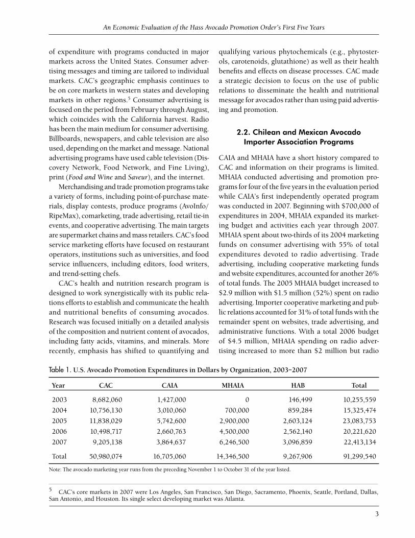
During its fi rst fi ve years of operation, HAB col-lected assessments totaling $98.67 million and rebated $77.6 million—$38.64 million to CAC, $20.54 million to the Chilean Avocado Importers’ Associa-tion (CAIA), and $18.42 million to the Mexican Hass Avocado Importers’ Association (MHAIA). Total fi ve-year promotional expenditures were $50.98 million by CAC, $16.71 million by CAIA, $14.35 million by MHAIA, and $9.27 million by HAB, amounting to a total of $91.3 million spent on Hass avocado promo-tion in the U.S. market.
Even though the HAPRIO is only fi ve years old, pro-motion of avocados in the U.S. market by California producers provides signifi cant program experience on which to build. Using a state marketing order, the California avocado industry conducted generic adver-tising and promotion programs between 1962 and 1977 and has operated under provisions of CAC since September 1978. The California industry spent more than $334 million (in 2007 dollars) on advertising,
promotion, and related services from initiation of the program in 1962 through 2002.2 Total promotion expenditures by the California industry, including HAPRIO allocations for 2003–2007, were almost $398 million (in 2007 dollars). Additional promotional expenditures in the U.S. market by HAB, MHAIA, and CAIA from initiation of HAPRIO assessments in 2003 through the end of the 2007 marketing year totaled almost $42 million (in 2007 dollars).
Hass avocado promotion programs take many forms. CAC allocates the majority of its funds to consumer advertising and merchandising/trade pro-motions.3 Signifi cant expenditures are also made on food service, public relations, nutrition, and internet marketing programs. CAIA contracted with CAC to conduct its marketing/promotion programs for the fi rst four years (from inception through the 2006 marketing year). In 2007 CAIA began conducting its own programs. MHAIA did not conduct any pro-motion programs in 2003 but has been active since 2004. HAB expenditures have emphasized national market communications and industry information programs.4
Annual promotion expenditures by the three associations are shown in Table 1. The California data are for marketing programs only (industry programs and administration are excluded) and HAB’s data are for marketing communications only (informa-tion programs and administration are excluded). All organizational expenditures are reported for Chile and Mexico.
2.1. California Avocado Commission Programs
CAC typically allocates about 70% of its revenue from producer assessments to its marketing programs. Consumer advertising is the leading activity in terms
2 The U.S. avocado marketing year runs from November 1 through October 31 of the following year. We use the convention of referring to the marketing year as the latter year; for example, we refer to November 1, 2002, through October 31, 2003, as 2003.3 CAC also collects additional funds from production of California Hass and other types of avocados to support its industry programs and other activities.4 Information in this section is based on each organization’s annual business or marketing plans and budgets as available.
An Economic Evaluation of the Hass Avocado Promotion Order’s First Five Years
3
of expenditure with programs conducted in major markets across the United States. Consumer adver-tising messages and timing are tailored to individual markets. CAC’s geographic emphasis continues to be on core markets in western states and developing markets in other regions.5 Consumer advertising is focused on the period from February through August, which coincides with the California harvest. Radio has been the main medium for consumer advertising. Billboards, newspapers, and cable television are also used, depending on the market and message. National advertising programs have used cable television (Dis-covery Network, Food Network, and Fine Living), print (Food and Wine and Saveur), and the internet.
Merchandising and trade promotion programs take a variety of forms, including point-of-purchase mate-rials, display contests, produce programs (AvoInfo/RipeMax), comarketing, trade advertising, retail tie-in events, and cooperative advertising. The main targets are supermarket chains and mass retailers. CAC’s food service marketing efforts have focused on restaurant operators, institutions such as universities, and food service infl uencers, including editors, food writers, and trend-setting chefs.
CAC’s health and nutrition research program is designed to work synergistically with its public rela-tions efforts to establish and communicate the health and nutritional benefits of consuming avocados. Research was focused initially on a detailed analysis of the composition and nutrient content of avocados, including fatty acids, vitamins, and minerals. More recently, emphasis has shifted to quantifying and
qualifying various phytochemicals (e.g., phytoster-ols, carotenoids, glutathione) as well as their health benefi ts and effects on disease processes. CAC made a strategic decision to focus on the use of public relations to disseminate the health and nutritional message for avocados rather than using paid advertis-ing and promotion.
2.2. Chilean and Mexican Avocado Importer Association Programs
CAIA and MHAIA have a short history compared to CAC and information on their programs is limited. MHAIA conducted advertising and promotion pro-grams for four of the fi ve years in the evaluation period while CAIA’s fi rst independently operated program was conducted in 2007. Beginning with $700,000 of expenditures in 2004, MHAIA expanded its market-ing budget and activities each year through 2007. MHAIA spent about two-thirds of its 2004 marketing funds on consumer advertising with 55% of total expenditures devoted to radio advertising. Trade advertising, including cooperative marketing funds and website expenditures, accounted for another 26% of total funds. The 2005 MHAIA budget increased to $2.9 million with $1.5 million (52%) spent on radio advertising. Importer cooperative marketing and pub-lic relations accounted for 31% of total funds with the remainder spent on websites, trade advertising, and administrative functions. With a total 2006 budget of $4.5 million, MHAIA spending on radio adver-tising increased to more than $2 million but radio
Table 1. U.S. Avocado Promotion Expenditures in Dollars by Organization, 2003–2007
Year CAC CAIA MHAIA HAB Total
2003 8,682,060 1,427,000 0 146,499 10,255,559
2004 10,756,130 3,010,060 700,000 859,284 15,325,474
2005 11,838,029 5,742,600 2,900,000 2,603,124 23,083,753
2006 10,498,717 2,660,763 4,500,000 2,562,140 20,221,620
2007 9,205,138 3,864,637 6,246,500 3,096,859 22,413,134
Total 50,980,074 16,705,060 14,346,500 9,267,906 91,299,540
Note: The avocado marketing year runs from the preceding November 1 to October 31 of the year listed.
5 CAC’s core markets in 2007 were Los Angeles, San Francisco, San Diego, Sacramento, Phoenix, Seattle, Portland, Dallas, San Antonio, and Houston. Its single select developing market was Atlanta.

Giannini Foundation Research Report 351
4
advertising’s total budget share decreased to 45%. Importer cooperative marketing, public relations, and trade advertising accounted for almost 32% of total expenditures in 2006. The major new expenditure of $498,000 was for a NASCAR sponsorship. With a total 2007 budget of $6,246,500, MHAIA spending on radio advertising increased slightly to $2,040,000 (32.7% of the total). With spending of $1.89 million, the share for importer cooperative marketing, public relations, websites, and in-store advertising was a little more than 27%. Spending on the NASCAR sponsorship and promotion increased to $1,423,500 (22.8%).
There is some annual information on CAIA market-ing programs while it contracted with CAC but only aggregate expenditure data for its independent 2007 program. Note also that CAIA data that are available are for the period during each season when avocados from Chile are exported to the United States rather than for the California marketing year. Information for the period August 2003 through February 2004 indi-cates that the CAIA marketing program conducted by CAC included radio advertising, public relations, and merchandising. Radio advertising accounted for about 85% of expenditures on all programs. Four three-week radio campaigns were conducted in 2003/04 in twelve selected markets: August 18 through September 8 (including Labor Day), September 29 through Octo-ber 20, November 10 through December 1 (including Thanksgiving), and December 29 through January 19, 2004 (leading up to the Super Bowl).6 CAIA conducted the same marketing programs in the same markets the following season (April 2004 through February 2005). Total spending for radio programs during this period was $3.3 million. CAIA marketing pro-grams from April 2005 through February 2006 were similar to the preceding two years with an emphasis on consumer radio advertising. Rather than the four three-week radio campaigns done previously, the 2005/06 campaign consisted of three three-week and two two-week programs. In 2007, CAIA also included television ads for general and Hispanic markets and sport and media promotion programs.
2.3. Hass Avocado Board Programs
HAB marketing programs fall under two major categories: information technology (InfoTech) and marketing communications (MarCom). InfoTech con-sists of AvoHQ.com on the internet and the Network Marketing Center, which are designed to exchange marketing and strategic information from all suppli-ers of Hass avocados to the U.S. market to improve the fl ow of fruit and maintain orderly marketing conditions. MarCom consists of consumer commu-nications, online marketing, trade communications, industry communications, and marketing research. The MarCom share of HAB’s budget has increased over time as the total HAB budget has increased and as the InfoTech program has become established. Initially in 2003, HAB spent $340,179 on InfoTech and $146,499 on MarCom. Expenditures grew for both programs in 2004 with $1,090,228 spent on InfoTech and $859,284 spent on MarCom. Consumer communications included Super Bowl and Cinco de Mayo promotions and public relations efforts that resulted in news releases with strong visibility. The website avocadocentral.com was established. MarCom became HAB’s major expenditure category in 2005 with a budget of almost $2.7 million while InfoTech projects had a budget of $746,000.
MarCom’s budget increased again to almost $3.5 million in 2006. Partnering with the Beef Checkoff and a Napa Valley winery, HAB collaborated to develop a 30-minute television program called “Hot Trends in Tailgating” that was aired on three cable networks (The Food Network, HGTV, and Fine Living Network). Six airings of the 30-minute show on each of the three networks were supplemented with 30-second con-sumer advertising spots that ran more than 100 times on four consecutive weeks on The Food Network, creating more than 27 million media impressions. The tailgating theme was continued in 2007 with a new partner (Miller Brewing) and a coordinated program with retailers, internet marketing, and public rela-tions. MarCom expenditures increased to almost $3.2 million while InfoTech expenditures were $750,000.
6 Thanksgiving, the Super Bowl, and Labor Day are holidays/events shown by Li (2007) to represent periods of high avocado consumption in the United States.

An Economic Evaluation of the Hass Avocado Promotion Order’s First Five Years
5
Avocados consumed in the United States before 1990 came largely from California production; export and import volumes were very small.
Estimated U.S. avocado consumption remained below a pound per capita until 1975 when a large California crop pushed consumption to 1.2 pounds per capita. Avocado imports slowly increased during the last half of the 1980s and fi rst exceeded 25 million pounds in 1990. Imports continued to expand through the 1990s and then exploded as Mexico gained access incrementally to the U.S. market. Imported avocados accounted for 26.1% of U.S. consumption in 1998 and reached 73.1% in 2007. Per capita consumption expanded with increased imports, reaching a record high of 3.45 pounds in 2006 and 2007. Estimated U.S. per capita avocado consumption for 1980–2007 by source of the avocados is shown in Figure 1, dem-onstrating the striking growth of imports in total and as a share of U.S. consumption.
Several factors are associated with increased U.S. avocado consumption. No doubt a key factor is the year round availability of good-quality avocados in the United States. Quality has been improved in part by industry-sponsored merchandising programs for produce personnel in supermarkets that stress the importance of proper ripening and having different maturity levels available for consumers. Industry promotion budgets have included nutrition programs for several years and have been successful in having avocados mentioned specifi cally as a recommended
fruit in diet plans and food pyramids such as the Mediterranean Diet Pyramid and the Atkins Lifestyle Food Guide Pyramid.
Industry studies have also examined demographic characteristics of avocado consumers. Cook (2003) described the typical U.S. avocado purchaser as a woman 25–54 years of age, having an income of $50,000 plus, upscale, college educated, working full/part time, and health conscious. The most fre-quent uses for avocados are for guacamole, as part of a Mexican side dish, in a salad, eaten plain, in a sandwich or burger, and as part of a non-Mexican entrée (Cook 2003).
HAB (2007) sponsored research examining U.S. Hispanic consumers that tended to confi rm some widely held industry perceptions, including that Hispanics buy signifi cantly more avocados than the average consumer. For the time period tracked, 97% of Hispanic shoppers bought avocados as compared to 49% of the general population. In addition, 60% of Hispanic shoppers purchased avocados weekly and the average purchase of 4.8 avocados was 58% greater than the average for consumers overall. Research reveals two distinct segments of the Hispanic market: U.S.-born Hispanics who speak English in the home and foreign-born Hispanics in Spanish-language-dom-inant households. Hispanics born in the United States are more aware of the Hass variety but purchase fewer avocados than their foreign-born counterparts.
3. AVOCADO CONSUMPTION IN THE UNITED STATES

Giannini Foundation Research Report 351
6
Figure 1. Annual U.S. Per Capita Avocado Consumption by Source, 1980–2007
Imports
Florida
California
3.5
3.0
2.5
2.0
1.5
1.0
0.5
01980 1982 1984 1986 1988 1990 1992 1994 1996 1998 2000 2002 2004 2006
pounds
year
An Economic Evaluation of the Hass Avocado Promotion Order’s First Five Years
7
This analysis benefi ts from a considerable base of prior research on the avocado market and avocado promotion. Previous studies provide
analytical models and empirical estimates for avocado demand parameters, demand responses to promotion programs, and acreage responses to price changes. We discuss this work and provide an updated analysis in this section.
4.1. Previous Studies
Carman and Green (1993) estimated equations for price and acreage responses as major components of a simulation model of the California avocado indus-try that was used to estimate the impact of generic advertising on acreage and returns over time. The price equation, calculated at mean values, yielded a price fl exibility of demand of –1.16 and a price fl exibility of advertising of 0.15.7 Carman and Cook (1996) used a revised and updated version of the Carman and Green model to examine possible impacts of avocado imports from Mexico on the California industry. The price equation, calculated at mean values, yielded a price fl exibility of demand of –1.53 and an advertising fl exibility of demand of 0.28.
Carman and Craft (1998) estimated both annual and monthly price equations for California avocados in a study of the returns to CAC promotion programs. The estimated annual fl exibilities of demand for price and advertising were –1.33 and 0.13, respectively. Estimated monthly fl exibilities of demand for price and advertising were –1.54 and 0.137, respectively.8 They estimated that California avocado producers achieved an annual average benefi t-cost ratio of 2.84 for the 34-year period covered by their analysis.
Short-term returns, based on an assumption of fi xed supply, ranged from $5.25 to $6.35 per dollar spent on advertising.
The USDA’s Animal and Plant Health Inspection Service (APHIS) included an economic analysis of the potential economic impact of increased Hass avo-cado imports from Mexico in three reports issued on proposals to increase the number of states and time period for shipments of avocados from Mexico. In the 2001 and 2003 reports, APHIS used a price elasticity of demand of –0.86 (USDA 2001, 2003). For the 2004 study, the report used a price elasticity of demand of –0.57 (USDA 2004).9 APHIS did not consider the possible impacts of advertising and promotion on demand for avocados.
The most recent analysis of the impact of promo-tion on U.S. avocado demand, based on annual data from 1962 through 2003, estimated that importers could realize returns ranging from $2.09 to $3.26 per dollar of HAPRIO expenditures with net returns decreasing as imports increase (Carman 2006, p. 476). This study assumed that the effectiveness of importer promotion expenditures would be equivalent to the effectiveness of CAC expenditures.
4.2. Econometric Models of the Annual Demand for Avocados
Estimated U.S. avocado demand equations in the cited studies included variables for per capita sales, real prices, income, promotion expenditures, and share of the population that is Hispanic. Other possible demand-shift variables (such as prices of possible substitutes and complements for avocados) and fac-tors associated with trends in demand (including
4. MODELING ANNUAL DEMAND FOR AVOCADOS
7 The price fl exibility of demand (advertising) is the percent change in price due to a 1% increase in sales (advertising). Thus, a 1% increase in advertising expenditures, for example, was estimated to increase the California FOB price by 0.15%.8 The responsiveness of avocado demand to generic advertising found in these studies is consistent in magnitude to that found for several other California commodities. Alston et al. (2005, pp. 406–407), in their summary of commodity promotion programs, listed advertising fl exibilities of demand of 0.13 and 0.16 for eggs and strawberries, respectively, and advertising elasticities of demand as follows: table grapes, 0.16; dried plums, 0.05; almonds, 0.13; walnuts, 0.005; raisins, 0.029 in Japan and 0.133 in the United Kingdom. Kinnucan and Zheng (2005, pp. 262–263, 270) summarize estimated elasticities and benefi t-cost estimates for the dairy, beef, pork, and cotton promotion programs.9 The price elasticity of demand is the inverse of the fl exibility of demand estimated by Carman (2006) and others. Thus, all of these estimates are broadly consistent—demand for avocados is inelastic (or fl exible), meaning that a 1% increase in price causes less than a 1% reduction in the quantity demanded.
Giannini Foundation Research Report 351
8
increased seasonal availability of avocados due to imports, changing demographics, and the growing popularity of Mexican foods) have also been investi-gated but with limited success. Carman (2006, p. 472) introduced a variable for the percentage of Hispanics in the U.S. population as a measure of the impact of demographic changes and the increased demand for Mexican foods. He also examined use of variables to measure increased imports (and, hence, increased seasonal availability) and account for possible substi-tutes but none had a measurable impact on avocado demand.
Using the results of the previous studies and economic theory, we specifi ed annual demand for avocados in the United States as a function of several explanatory variables:
(1) Qat = f(Pat, At, Yt, Ht)
where the variables for a given crop year t are defi ned as follows.
• Qat is per capita U.S. sales (pounds per person) of avocados from all sources (California, Florida, and all imports) less exports from the United States.
• Pat is the average real FOB (farm) price of Califor-nia avocados.
• At is the real total value of avocado advertising and promotion expenditures.
• Yt is real per capita U.S. disposable income.
• Ht is the percentage of the total U.S. population that is Hispanic.
Prior to the creation of the HAPRIO, At consisted mainly of expenditures by CAC.
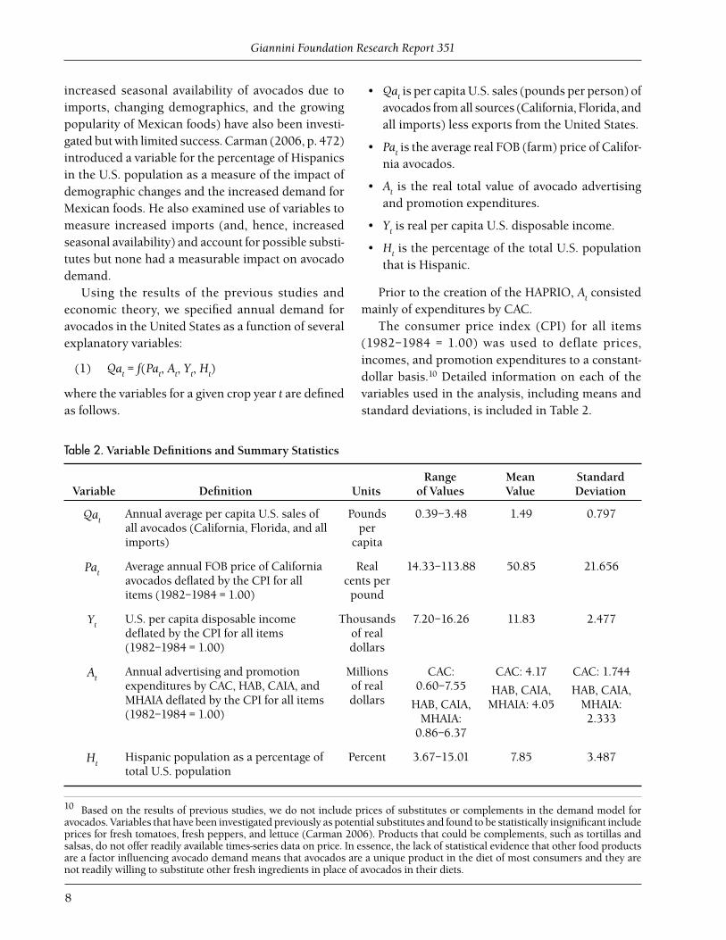
The consumer price index (CPI) for all items (1982–1984 = 1.00) was used to deflate prices, incomes, and promotion expenditures to a constant-dollar basis.10 Detailed information on each of the variables used in the analysis, including means and standard deviations, is included in Table 2.
Table 2. Variable Defi nitions and Summary Statistics
Variable Defi nition UnitsRange
of ValuesMean Value
Standard Deviation
QatAnnual average per capita U.S. sales of all avocados (California, Florida, and all imports)
Pounds per
capita
0.39–3.48 1.49 0.797
PatAverage annual FOB price of California avocados defl ated by the CPI for all items (1982–1984 = 1.00)
Real cents per
pound
14.33–113.88 50.85 21.656
Yt U.S. per capita disposable income defl ated by the CPI for all items (1982–1984 = 1.00)
Thousands of real dollars
7.20–16.26 11.83 2.477
AtAnnual advertising and promotion expenditures by CAC, HAB, CAIA, and MHAIA defl ated by the CPI for all items (1982–1984 = 1.00)
Millions of real dollars
CAC: 0.60–7.55
HAB, CAIA, MHAIA:
0.86–6.37
CAC: 4.17
HAB, CAIA, MHAIA: 4.05
CAC: 1.744
HAB, CAIA, MHAIA: 2.333
HtHispanic population as a percentage of total U.S. population
Percent 3.67–15.01 7.85 3.487
10 Based on the results of previous studies, we do not include prices of substitutes or complements in the demand model for avocados. Variables that have been investigated previously as potential substitutes and found to be statistically insignifi cant include prices for fresh tomatoes, fresh peppers, and lettuce (Carman 2006). Products that could be complements, such as tortillas and salsas, do not offer readily available times-series data on price. In essence, the lack of statistical evidence that other food products are a factor infl uencing avocado demand means that avocados are a unique product in the diet of most consumers and they are not readily willing to substitute other fresh ingredients in place of avocados in their diets.
An Economic Evaluation of the Hass Avocado Promotion Order’s First Five Years
9
Hispanics’ share of the U.S. population increased from 3.7% to 15.0% during the period of analysis, and U.S. Census Bureau projections show that the His-panic share will increase steadily, reaching 24.4% in 2050. Mexico is the world’s largest avocado producer and consumer with per capita avocado consumption recently reported at 8 kilograms or about 17.6 pounds annually compared to about 3.5 pounds per capita per year in the United States (USDA, Foreign Agricultural Service 2005). With approximately two-thirds of the U.S. Hispanic population originating from Mexico, this variable is intended to measure demographic change that may be related to avocado demand. The increasing Hispanic share of the U.S. population may also act as a proxy for the popularity of Mexican food and Mexican restaurants in the United States.
Consumer demand is inversely related to the price paid based on the “law of demand.” A basic question is which price to use in the demand analysis. Retail prices differ across stores and grower prices differ by avocado type and country of origin. For example, California avocados generally receive a higher price than avocados from Chile or Mexico. We used the California grower or FOB price because it is the only price series that is available for the entire period of the data analysis. Prices for avocados from different origins (California, Florida, Chile, and Mexico) and at different stages of the market chain (farm, wholesale, and retail) should move in unison as a consequence of the “law of one price” so the choice of the specifi c price series should be of little consequence.11 Another issue regarding price as an explanatory variable is its potential endogeneity. If prices and sales are deter-mined simultaneously in the market place, then price is endogenous and correlated with the error term in an estimation of equation 1, rendering the estimates inconsistent. We address the potential endogeneity of the FOB price later in this section.
4.3. Preliminary Data Analysis
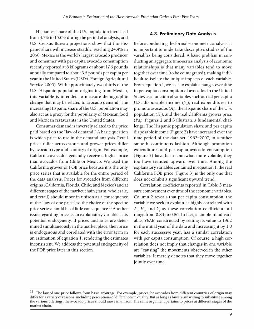
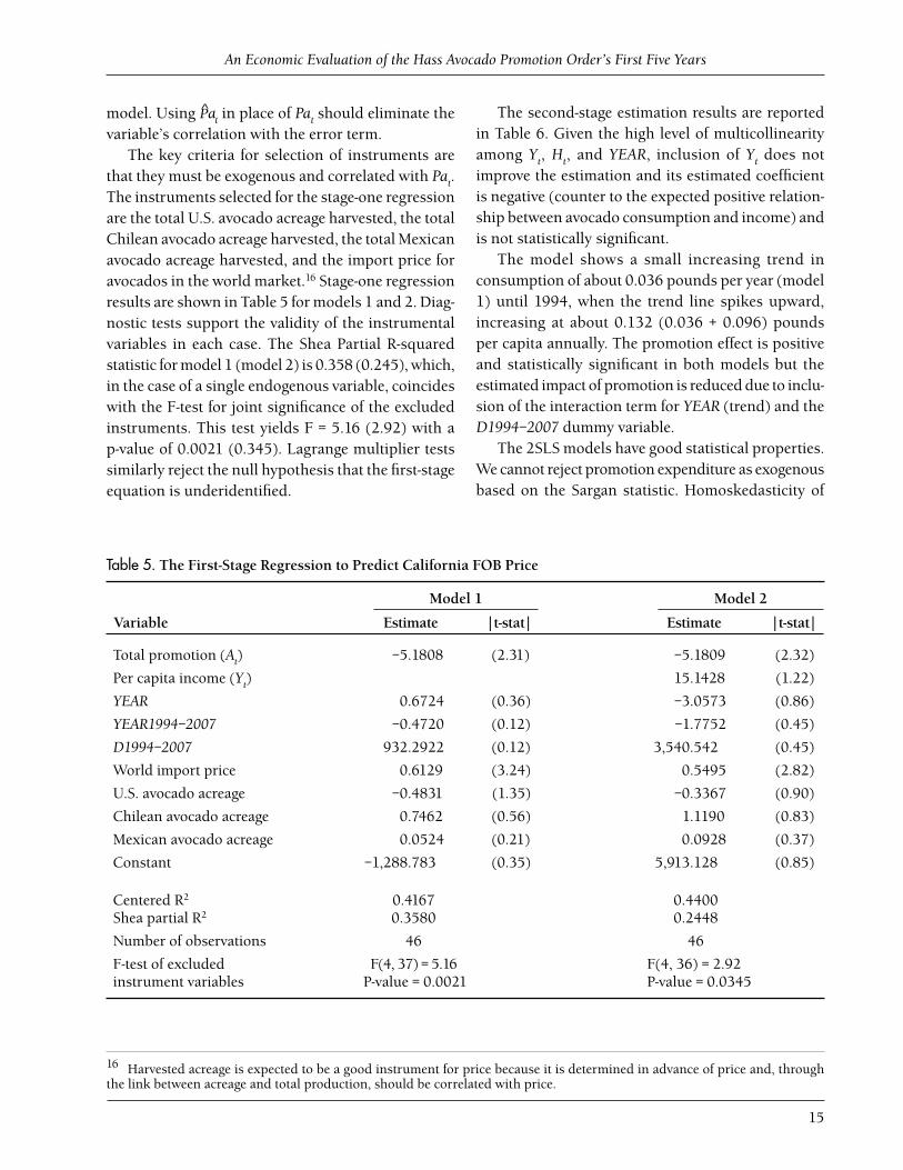
Before conducting the formal econometric analysis, it is important to undertake descriptive studies of the variables being considered. A basic problem in con-ducting an aggregate time-series analysis of economic relationships is that many variables tend to move together over time (to be cointegrated), making it dif-fi cult to isolate the unique impacts of each variable. From equation 1, we seek to explain changes over time in per capita consumption of avocados in the United States as a function of variables such as real per capita U.S. disposable income (Yt), real expenditures to promote avocados (At), the Hispanic share of the U.S. population (Ht), and the real California grower price (Pat). Figures 2 and 3 illustrate a fundamental chal-lenge. The Hispanic population share and per capita disposable income (Figure 2) have increased over the time period of the data set, 1962–2007, in a rather smooth, continuous fashion. Although promotion expenditures and per capita avocado consumption (Figure 3) have been somewhat more volatile, they too have trended upward over time. Among the explanatory variables contained in equation 1, the real California FOB price (Figure 3) is the only one that does not exhibit a signifi cant upward trend.
Correlation coeffi cients reported in Table 3 mea-sure comovement over time of the economic variables. Column 2 reveals that per capita consumption, the variable we seek to explain, is highly correlated with At, Ht, and Yt as these correlation coefficients all range from 0.83 to 0.86. In fact, a simple trend vari-able, YEAR, constructed by setting its value to 1962 in the initial year of the data and increasing it by 1.0 for each successive year, has a similar correlation with per capita consumption. Of course, a high cor-relation does not imply that changes in one variable are “causing” the movements observed in the other variables. It merely denotes that they move together jointly over time.
11 The law of one price follows from basic arbitrage. For example, prices for avocados from different countries of origin may differ for a variety of reasons, including perceptions of differences in quality. But as long as buyers are willing to substitute among the various offerings, the avocado prices should move in unison. The same argument pertains to prices at different stages of the market chain.

Giannini Foundation Research Report 351
10
year
Figure 2. Annual Per Capita Avocado Consumption, U.S. Per Capita Disposable Income, and the Percentage of the Population That Is Hispanic, 1962–2007
Quantity Consumed per Capita (pounds)
18
16
14
12
10
8
6
4
2
0
Percentage of the Population That Is Hispanic
U.S. Per Capita Disposable Income (dollars)
‘62 ‘64 ‘66 ‘68 ‘70 ‘72 ‘74 ‘76 ‘78 ‘80 ‘82 ‘84 ‘86 ‘88 ‘90 ‘92 ‘94 ‘96 ‘98 ‘00 ‘02 ‘04 ‘06
Figure 3. Annual Per Capita Avocado Consumption, FOB Price, and Promotion Expenditure, 1962–2007
‘62 ‘64 ‘66 ‘68 ‘70 ‘72 ‘74 ‘76 ‘78 ‘80 ‘82 ‘84 ‘86 ‘88 ‘90 ‘92 ‘94 ‘96 ‘98 ‘00 ‘02 ‘04 ‘06year
Total Expenditure (million dollars)
California Avocado Commission Promotion Expenditure (million dollars)
Quantity Consumed Per Capita (pounds)
California Price (cents/pound in real terms)
14
13
12
10
9
8
7
6
5
4
3
2
1
0

An Economic Evaluation of the Hass Avocado Promotion Order’s First Five Years
11
change over time. In other words, there may be struc-tural breaks in the data. This possibility is especially relevant for avocados given the signifi cant changes that have occurred in the industry over the 1962–2007 period of analysis in terms of rapidly escalating imports and the availability of product year round. Examination of the plot of per capita consumption over time in Figure 3 reveals two potential disruptions in the upward trend in per capita consumption—an upward shift in consumption between 1980 and 1981 and a downward shift in consumption between 1993 and 1994. Furthermore, following the decline in per capita consumption between 1993 and 1994, the upward trend in consumption from 1994 onward has a higher trajectory than those of the preceding years, no doubt refl ecting, at least in part, the progressive opening of U.S. markets to Mexican imports that began in 1997. A fundamental issue in the demand modeling is how to handle these structural shifts in consumption and the revised trend in consumption that began in 1994. If we do not account for these shifts through separate intercept-shift and trend variables and instead allow the changes in per capita consump-tion to be explained by the variables in equation 1, the estimated impact of the promotion variable is much greater, as is its statistical signifi cance. These results are presented next.
Also important to observe is that Yt and Ht are both highly correlated with YEAR as the correlation coef-fi cients are 0.97 and 0.99 respectively. In essence, over the 1962–2007 period of our data, Ht and Yt each have increased over time in a manner that can be almost perfectly predicted with a linear trend variable. Of course, Ht and Yt are also highly correlated with each other. Real promotion expenditures (At), while quite highly correlated with Ht, Yt, and YEAR, exhibit some independent comovement that is manifested by cor-relation coeffi cients with these three variables ranging from 0.74 to 0.77.12 This is favorable information given the purposes of the study because the independence of movement of At creates the potential to isolate the impact of promotion on avocado consumption rela-tive to impacts of the other variables. However, the extremely high correlation among Ht, Yt, and YEAR means that there is no opportunity to isolate their individual impacts.
4.4. Structural Breaks in Per Capita Consumption
Among the challenges in estimating an annual demand model is that the fundamental economic relationships linking the variable of interest, per capita consumption in our case, to potential explanatory variables may
12 Formal tests for the time-series properties of the model variables were also conducted. These included tests of the null hypothesis that a variable is stationary (i.e., a variable that reverts to a constant mean and does not exhibit a deterministic trend) against the alternative hypothesis that the variable has a unit root (i.e., the variable has no mean and follows a “random walk”). Detailed results of these tests are available from the authors. Briefl y, the California grower price, Pat, has no signifi cant trend and is covariance-stationary (i.e., stationary without a deterministic trend). All of the other variables (per capita consumption, real promotion expenditure, real per capita disposable income, and percent of the population that is Hispanic) have a statistically signifi cant trend that is apparent from examination of Figures 2 and 3. Per capita consumption and real promotion expendi-ture are trend-stationary (stationary after removal of a linear trend) while real per capita disposable income and percent of the population that is Hispanic each contain a unit root.
Table 3. Correlation Coeffi cients for the Demand Model
Qat Pat YEAR At Ht Yt
Per capita consumption (Qat) 1.00
Real California price (Pat) –0.50 1.00
YEAR 0.83 –0.15 1.00
Real total promotion expenditures (At) 0.86 –0.25 0.74 1.00
Hispanic share of population (Ht) 0.84 –0.15 0.97 0.75 1.00
Real per capita disposable income (Yt) 0.83 –0.12 0.99 0.77 0.95 1.00

Giannini Foundation Research Report 351
12
4.5. Estimated Annual Demand Relationships
Various demand functions based on equation 1 are estimated using 46 annual observations for the mar-keting years 1962 through 2007. The key objective is to determine the impact of total advertising and promo-tion programs on annual U.S. demand for avocados. Results from the alternative estimations are presented in Table 4. All of the estimations reported in Table 4 are conducted via ordinary least squares (OLS).
Several conclusions immediately follow from examination of Table 4. First, the overall explanatory power of the model is very high as measured by the adjusted R-square statistic, which measures the pro-portion of total variation in per capita consumption from 1962 through 2007 that is “explained” by the variables included in the model. Adjusted R-squares vary from about 0.92 to nearly 0.99 for the alternative models presented in the table.
Second, price is inversely related to per capita consumption in a way that is signifi cant statistically and robust to alternative model specifi cations. This result is, of course, consistent with prior studies and simply affi rms the law of demand but is gratifying nonetheless as an indication of an econometric model that is working properly. The estimated price elasticity of demand, evaluated at the data means, ranges from –0.41 to –0.46 depending on the model specifi cation. Thus, demand is in the inelastic range, meaning that a 1% increase in production causes roughly a 2% decrease in the FOB price when other factors are held constant.13
Third, high correlation (multicollinearity) among the variables Yt, Ht, and YEAR makes it impossible to estimate the individual effects of these variables on consumption. Recall that each of these variables is almost perfectly correlated with the other two. Thus, although we know from economic theory, past research, and basic information on the avocado industry that per capita consumption is likely to be positively related to per capita income and to the His-panic share of the U.S. population, it is not possible to isolate these two effects or, for that matter, to separate
their effects from a simple trend variable that could be capturing the effects of both Yt and Ht and other omitted variables affecting consumption.
This multicollinearity among Yt, Ht, and YEAR manifests itself in terms of estimated effects for each of these variables being unstable and highly sensitive to model specifi cation. For example, model 3 shows an inverse (and statistically insignifi cant) effect between Ht and Qat and also between YEAR and Qat. But these results are due merely to the statistical program imputing all of the impact of these three upward-trending variables to Yt in this model. In essence, due to their high multicollinearity, this attribution of impact is almost arbitrary. This can be seen in terms of the sensitivity of the results for these variables to minor changes in the model specifi cation. Importantly, because our main interest is in evaluating the effect of promotion, this inability to separate impacts due to Yt, Ht, and YEAR does not constitute a signifi cant limitation on the analysis.
Fourth, promotion has had a positive effect on demand that is statistically signifi cant for all models presented in Table 4. However, the magnitude of the promotion impact hinges on whether we account separately for the shift in per capita consumption that occurred between 1993 and 1994 and the increasing trend line for per capita consumption that began in 1994 and continues through the data set. The downward shift in per capita consumption is captured by the dummy variable D1994–2007, which is negative and statistically signifi cant in models 3 and 4. The greater trend upward in consumption that begins in 1994 is captured by the trend variable YEAR1994–2007, which is 1994 in the year 1994, increases by 1.0 for each subsequent year, and is zero for all years preceding 1994. Importantly, this change in trend cannot be explained by the other three vari-ables in the model (Yt, Ht, and YEAR) that are each trending upward smoothly through time. All three of those variables are included in model 3 and Yt and Ht are included in model 4. YEAR1994–2007 is positive and statistically signifi cant despite the presence of these other variables.
13 Though the estimate of price-inelastic demand in this study is lower (more inelastic) than those from prior studies, the es-timate remains consistent with the other studies of avocado demand due to higher rates of avocado consumption in the United States that began in the 1990s and have continued to the present, moving consumption down the demand curve into more inelastic regions.

An Economic Evaluation of the Hass Avocado Promotion Order’s First Five Years
13
The one variable in the model that can account, at least partially, for this increase in the consumption trend line is total promotion, which also exhibits an increasing rate of trend beginning about this same time and escalates especially rapidly with the creation of the HAPRIO. Thus, introducing separate shift (D1994–2007) and trend (YEAR1994–2007) variables to account for this evident change in per capita consumption eliminates roughly half of the estimated impact of the promotion variable. This is demon-strated by a comparison of the results from models 1 and 2 with the results of models 3 and 4. Promotion effects are nonetheless positive and statistically signifi -cant even in models 3 and 4. The estimated elasticity of demand with respect to promotion ranges from 0.148 to 0.372 depending on the model specifi cation.
The upper end of this range is high relative to prior estimates for the avocado industry and relative to other promotion studies generally. The lower end of the range is very consistent with prior estimates for avocados and in general.
We do not consider it possible to obtain a reliable separate estimate of the impact of promotion expen-ditures funded by HAB (i.e., expenditures in the last fi ve years) using an annual model. The main problem is that the creation of HAB was stimulated in large part by the rapid increase in avocado imports into the United States and the growing free-rider problem caused by importers not contributing to advertising programs funded through CAC. Thus, HAB’s naissance and commencement of funding programs under its auspices are associated with rapidly rising per capita
Table 4. Estimated Annual Demand Models: Ordinary Least Squares
Model 1 Model 2 Model 3 Model 4
Base Model Base Model + TrendModel 2 + Structural Break for 1994–2007
Model 3 without YEAR
Variable Estimate |t-stat| Estimate |t-stat| Estimate |t-stat| Estimate |t-stat|
California FOB price (Pat)
–0.0120[–0.414]
(7.48) –0.0125[–0.431]
(7.32) –0.0132[–0.455]
(8.69) –0.0131[–0.451]
(8.66)
Per capita income (Yt)
0.0739[0.592]
(1.56) 0.1782[1.429]
(1.43) 0.1904[1.526]
(2.88) 0.1389[1.114]
(3.97)
Hispanic share of population (Ht)
0.0609 (1.87) 0.0798 (2.06) –0.0103 (0.15) 0.2878 (0.56)
Total promotion (At)
0.1192[0.372]
(5.79) 0.1110[0.347]
(4.93) 0.0475[0.148]
(2.04) 0.0562[0.176]
(2.66)
YEAR –0.0230 (0.91) –0.0001 (0.92)
YEAR1994–2007 0.0902 (3.59) 0.0795 (3.58)
D1994–2007 –180.2921 (3.60) –158.9093 (3.59)
Constant 0.1850 (0.58) 44.485 (0.91)
Adjusted R2 0.9192 0.9188 0.9879 0.9879
Note: Absolute t-statistics are indicated in parentheses; elasticities evaluated at data means are in brackets.

Giannini Foundation Research Report 351
14
consumption of avocados in the United States. Any variables created to measure HAB’s influence on consumption (apart from the general infl uence over time of promotion as measured by At) will necessarily capture the rising trend in consumption much in the same way that it is captured presently by the variable YEAR1994–2007 in models 3 and 4. The creation of HAB occurred essentially simultaneously with the rapid increase in imports and associated increase in domestic consumption. As a result, we cannot impute a causal relationship from HAB’s creation and com-mencement of its funding programs to the increase in per capita consumption. Again, the industry’s ability to withstand the rapid escalation of imports without enduring drastic decreases in real prices demonstrates that demand grew substantially over this period and the analysis suggests that this demand growth is at least partially due to promotion.
4.6. Diagnostic Checks of Annual Demand Models
Here we report briefl y on diagnostic tests of the mod-els reported in Table 4. These tests are important in determining the confi dence that we can have in the estimated results.14 The ability to attach confi dence intervals to estimated effects and conduct statisti-cal tests (such as whether the effect of promotion is statistically different from zero) depends on the properties of the estimated residuals (actual per capita consumption in year t minus predicted per capita consumption in year t). The tests confi rm that the estimated residuals are homoskedastic (i.e., they have a constant variance) and distributed normally. Both are desirable properties that support the use of the model for hypothesis tests.
The residuals do, however, reveal some evidence of serial correlation, i.e., the expected value of the error in period t is a function of the error in period t – 1. The estimated coeffi cients are consistent in the presence of serial correlation but the estimated stan-dard errors (used to construct the t-statistics) need
to be adjusted to correct for the presence of serial correlation. A more insidious problem is that serial correlation of the errors may create problems of endo-geneity of the explanatory variables.15 Elimination of serial correlation in the errors may thus eliminate some endogeneity problems.
Among the explanatory variables in the model, two are candidates for being endogenous: Pat and At. The California FOB price may be endogenous because it could be determined contemporaneously with consumption through the ordinary workings of the market. Promotion expenditures could be endogenous because the total budget for promotion is determined by the check-off rate multiplied by the total production of avocados that are subject to the check-off. Realistically, there is a lag between realiza-tion of production and consumption, collection of the check-off funds, preparation of marketing budgets, and actual expenditures on promotion so it is reason-able to believe that promotion expenditures during year t were determined for the most part by production in year t – 1. Therefore, At is exogenous unless errors are serially correlated.
Our strategy is to address the endogeneity of the California FOB price using the two-stage least squares (2SLS) estimation procedure because good instruments for it are available as described in the next subsection. Unless there is strong evidence of autocorrelated residuals in the 2SLS estimation, we can be relatively confi dent that At is exogenous for the reasons noted.
4.7. Two-Stage Least Squares Estimation
Based on the OLS results, two models were consid-ered in the 2SLS estimation. Model 1 includes only YEAR to capture the linear trend effect present in all three variables. Model 2 adds Yt as an explanatory variable. The fi rst-stage estimation involves regressing Pat on a set of exogenous instruments. The second stage involves using the predicted value, P̂at, in place of actual Pat and re-estimating the annual demand
14 Details on various diagnostic tests are available from the authors.15 Endogeneity is more likely in the presence of serially correlated errors because an explanatory variable with a value in period t that is determined, say, by events in period t – 1 (and would thus be uncorrelated with the error term in period t in the absence of serial correlation) becomes correlated with the error term in period t and, hence, endogenous if the error term is serially correlated.
An Economic Evaluation of the Hass Avocado Promotion Order’s First Five Years
15
model. Using P̂at in place of Pat should eliminate the variable’s correlation with the error term.
The key criteria for selection of instruments are that they must be exogenous and correlated with Pat. The instruments selected for the stage-one regression are the total U.S. avocado acreage harvested, the total Chilean avocado acreage harvested, the total Mexican avocado acreage harvested, and the import price for avocados in the world market.16 Stage-one regression results are shown in Table 5 for models 1 and 2. Diag-nostic tests support the validity of the instrumental variables in each case. The Shea Partial R-squared statistic for model 1 (model 2) is 0.358 (0.245), which, in the case of a single endogenous variable, coincides with the F-test for joint signifi cance of the excluded instruments. This test yields F = 5.16 (2.92) with a p-value of 0.0021 (0.345). Lagrange multiplier tests similarly reject the null hypothesis that the fi rst-stage equation is underidentifi ed.
The second-stage estimation results are reported in Table 6. Given the high level of multicollinearity among Yt, Ht, and YEAR, inclusion of Yt does not improve the estimation and its estimated coeffi cient is negative (counter to the expected positive relation-ship between avocado consumption and income) and is not statistically signifi cant.
The model shows a small increasing trend in consumption of about 0.036 pounds per year (model 1) until 1994, when the trend line spikes upward, increasing at about 0.132 (0.036 + 0.096) pounds per capita annually. The promotion effect is positive and statistically signifi cant in both models but the estimated impact of promotion is reduced due to inclu-sion of the interaction term for YEAR (trend) and the D1994–2007 dummy variable.
The 2SLS models have good statistical properties. We cannot reject promotion expenditure as exogenous based on the Sargan statistic. Homoskedasticity of
16 Harvested acreage is expected to be a good instrument for price because it is determined in advance of price and, through the link between acreage and total production, should be correlated with price.
Table 5. The First-Stage Regression to Predict California FOB Price
Model 1 Model 2
Variable Estimate |t-stat| Estimate |t-stat|
Total promotion (At) –5.1808 (2.31) –5.1809 (2.32)
Per capita income (Yt) 15.1428 (1.22)
YEAR 0.6724 (0.36) –3.0573 (0.86)
YEAR1994–2007 –0.4720 (0.12) –1.7752 (0.45)
D1994–2007 932.2922 (0.12) 3,540.542 (0.45)
World import price 0.6129 (3.24) 0.5495 (2.82)
U.S. avocado acreage –0.4831 (1.35) –0.3367 (0.90)
Chilean avocado acreage 0.7462 (0.56) 1.1190 (0.83)
Mexican avocado acreage 0.0524 (0.21) 0.0928 (0.37)
Constant –1,288.783 (0.35) 5,913.128 (0.85)
Centered R2 0.4167 0.4400Shea partial R2 0.3580 0.2448
Number of observations 46 46
F-test of excluded F(4, 37) = 5.16 F(4, 36) = 2.92instrument variables P-value = 0.0021 P-value = 0.0345

Giannini Foundation Research Report 351
16
Table 6. Estimated Annual Demand Models: Two-Stage Least Squares
Model 1 Model 2
Variable Estimate |t-stat| Estimate |t-stat|
Predicted California FOB price –0.0117 (5.64) –0.0109 (3.86)
Per capita income (Yt) –0.0698 (0.53)
Total promotion (At) 0.0492 (2.34) 0.0527 (2.32)
YEAR 0.0362 (8.20) 0.0494 (1.92)
YEAR1994–2007 0.0964 (5.99) 0.0988 (5.86)
D1994–2007 –192.778 (5.99) –197.587 (5.86)
Constant –69.899 (8.05) –95.385 (1.93)
Centered R2 0.96 0.96Number of observations 46 46
residuals is not rejected based on the Pagan-Hall test and the hypothesis that the residuals are not auto-correlated of order 1 cannot be rejected under any versions of the Cumby-Huizinga tests.
Finally, based on the Ramsey/Peseran-Taylor Reset test, we cannot reject the null hypothesis that the true relationship among the variables is linear.17
4.8. Summary
As illustrated in Figures 1 and 4, imports of avocados into the United States increased dramatically begin-ning in the early 1990s and have continued to increase since. The evidence from this study and prior studies suggests that avocado demand in the United States is price inelastic. Thus, a given percentage increase in supply will cause a greater and opposite percentage change in price. Rapid supply growth in the presence of inelastic demand can be a disastrous combination
for an industry in the absence of demand growth. Yet, as the record shows (Figure 3), the real farm price in California has not fallen appreciably during this period of rapidly escalating imports, meaning that demand has expanded suffi ciently to keep real prices relatively stable.18
In general, demand for food in the United States grows very slowly. In a high-income nation, most people have suffi cient food to eat. Therefore, as their incomes and expenditures grow, little of the incre-mental expenditure goes for food. Unquestionably, avocado demand in the United States has expanded during this period at a much faster rate than demand for food generally. The only variable in our model that is capable of explaining the increasing trend line is promotion. For example, per capita income and the Hispanic share of the population do not exhibit a similar increase in trend lines.
17 Evaluations of commodity promotion programs often specify a nonlinear effect between promotion expenditure and demand. The economic basis for this specifi cation is that promotion must eventually have a diminishing return. Otherwise, in theory, it would be possible to expand demand indefi nitely by spending ever increasing amounts of money to promote the product. However, such diminishing returns may not be observed if the actual amount of expenditure is less than the amount that coincides with the onset of diminishing returns. We estimated various models with a nonlinear relationship between promotion expenditure and per capita consumption but none improved the model’s performance. This outcome is consistent with the results from the Ramsey/Peseran-Taylor Reset test.18 To be more precise, a regression of real California FOB price for 1994 through 2007 on a constant and a linear trend results in the following equation: P̂at = 58.86 – 1.095YEAR. The absolute t-statistic on the YEAR coeffi cient is 1.63. Thus, the real price is estimated to have fallen by about 1¢ per year but the effect is not statistically signifi cant at 90% or higher confi dence levels.

An Economic Evaluation of the Hass Avocado Promotion Order’s First Five Years
17
Figure 4. Avocado Supply, Imports, and Domestic Production in the United States, 1962–2007
Notes: Total U.S. avocado consumption equals the sum of avocado production in California and Florida and total avocado imports minus total avocado exports. Total U.S. avocado production equals the sum of avocado production in California and Florida.
‘62 ‘64 ‘66 ‘68 ‘70 ‘72 ‘74 ‘76 ‘78 ‘80 ‘82 ‘84 ‘86 ‘88 ‘90 ‘92 ‘94 ‘96 ‘98 ‘00 ‘02 ‘04 ‘06
800
700
600
500
400
300
200
100
0
million pounds
Total Imports to the United States
Imports from Chile
Imports from Mexico
year

Giannini Foundation Research Report 351
18
5. BENEFIT-COST ANALYSIS
The econometric analysis reported in section 4 presents strong evidence that generic pro-motion of avocados has worked to increase
the demand for avocados in the United States. The additional question to ask, however, is whether the promotion expenditures have paid off in the sense of yielding benefi ts to producers from demand enhance-ment that exceed the money expended to fund the programs. We address that question in this section.
5.1. Benefit-Cost Analysis in Promotion-Evaluation Studies
Two types of benefi t-cost ratios are relevant in promo-tion-evaluation analyses—average benefi t-cost ratios (ABCRs) and marginal benefi t-cost ratios (MBCRs). For producers, the ABCR from a promotion program consists of the total incremental profi t to produc-ers generated by the program over a specifi ed time interval divided by the total incremental cost borne by producers to fund the program. Both the profi t and cost streams should be properly discounted or compounded to a common point in time. The ABCR is the key measure of whether a program succeeded with an ABCR that is greater than or equal to 1.0 defi n-ing success.19 The MBCR measures the incremental profi t to producers generated from a small expansion or contraction of a promotion program. That is, the MBCR determines whether expansion of the promo-tion program would increase producer profi ts. An MBCR that is greater than 1.0 indicates a program that could have been profi tably expanded.
In general, the ABCR does not equal the MBCR because promotion is usually modeled as having a nonlinear effect on demand. For example, the square-root function is often used to represent the relationship between promotion and demand and this functional form guarantees a declining effect of marginal promotion dollars on sales (e.g., Alston et al. 1997). Thus, the ABCR is greater than the MBCR for the square-root model. As discussed in section 4, we
utilize a linear model to depict the functional relation-ship between demand and promotion expenditures and this relationship is not rejected by econometric tests. For the linear model, the ABCR equals the MBCR and, thus, the two questions—was the program profi t-able and could it have been profi tably expanded—are one and the same.
Our strategy is to simulate the impact of a small hypothetical increase in HAB’s assessment rate from the current level of $0.025 to $0.030 per pound (an increase of one-half cent per pound) and estimate the benefi ts and costs to avocado growers from that assessment expansion. The ratio of estimated benefi ts to costs is then the estimated MBCR. Given that the functional relationship is linear, it is also an estimate of the entire program’s ABCR.
The simulation framework is depicted in Figure 5. The model begins with demand and supply func-tions for avocados that depict the current market. Thus, demand, D, is total U.S. demand as estimated in section 4 on a per capita basis. Supply, S, is total supply to the U.S. market from all sources. The precise “shape” of this supply relationship is a matter of some importance for the simulation model and will be dis-cussed shortly. Under the current program, total U.S. consumption given functions S and D is QA and price is PA. Implementation of a one-half cent expansion in the program assessment has the effect of increasing producer costs by one-half of a cent, which shifts sup-ply upward to curve S′ as depicted in Figure 5.
The additional funds generated by the program expand the level of demand by an amount equal to the incremental funds generated by the assessment multiplied by the estimated marginal impact of the promotion expenditure on demand. The incremental funds are simply the change in assessment multiplied by total shipments to the U.S. market and the esti-mated marginal impact is the regression coeffi cient for the promotion variable, At, which is reported for alternative model specifi cations in Tables 4 and 6. The new demand curve is illustrated in Figure 5 by D′. The
19 Because the streams of both benefi ts and costs are discounted or compounded at an interest rate intended to represent the industry’s opportunity cost in terms of alternative investments, the benefi t-cost ratio is automatically adjusted for the opportunity cost of the funds used to support promotion.

An Economic Evaluation of the Hass Avocado Promotion Order’s First Five Years
19
new market equilibrium is found at the intersection of curves S′ and D′ at point A in Figure 5. The equilibrium price has risen to P′ and sales have risen to Q′.
Producer benefi ts from the hypothetical expansion of the promotion program are measured in terms of producer surplus, PS, which is the same as producers’ variable profi ts (i.e., the producer surplus equals the producer price multiplied by output minus the vari-able production costs associated with producing and selling the output). In Figure 5, PS in the absence of the promotion program is measured by the revenue rectangle PAxQA minus the area below the supply curve (the triangle 0CQA), which represents the total variable costs associated with producing and selling output QA.
We seek to measure the change in producer surplus associated with the hypothetical expansion of the promotion program. In Figure 5, PS after the pro-gram expansion is PS′ = P′Q′ – 0BQ′ but we must also account for the additional promotion expenditure, which is the rectangle PA′P′AB = (P′ – PA′)Q′. Thus, the net increase in surplus to producers from expansion of the promotion program is ΔPS = PS′ – (P′ – PA′)Q′, which is represented by the shaded area in Figure 5.
Three pieces of information are necessary to estimate ΔPS: (1) estimates of the marginal impact of
promotion expenditures on demand, (2) estimates of the slope or price elasticity, εD, of demand, and (3) estimates of the slope or price elasticity, εS, of supply of avocados to the U.S. market. We have estimates of the fi rst two from the econometric models sum-marized in Tables 4 and 6 but lack an estimate of εS. Most promotion evaluation studies do not attempt to estimate the elasticity of the supply relationship. Sup-ply functions are diffi cult to estimate empirically and the elasticity varies by the length of run (time frame) under consideration. For example, supply becomes more elastic (responsive to price) in the long run as more productive inputs become variable to producers. Supply analysis is particularly diffi cult for perennial crops because the analyst must normally specify a dynamic model containing equations for plantings, removals, bearing acreage as a function of plantings and removals, and yield.
Carman and Craft (1998) analyzed supply response in the California avocado industry. Avocado supply to the United States is now complicated rela-tive to the time period analyzed by Carman and Craft by the fact that both Chile and Mexico are important suppliers to the U.S. market as well as to their own domestic markets and other export markets. Thus, the Chilean and Mexican supply to the U.S. market
is a residual supply that is based on total production and domestic demand in each country and demand from all importing coun-tries except the United States.
The alternative and increas ing ly popular approach to studying the supply relationship is to estimate benefi t-cost ratios for a range of plausible values for εS. If the conclu-sions are robust across the range of supply elasticity values chosen, there is little need to worry about choosing among the plau-sible alternative values. Examples of the alternative
Figure 5. Avocado Promotion Simulation Model
QA Q′
PA
S′S
D′D
P′P′A
0.5
BC
A
Pat
Giannini Foundation Research Report 351
20
approach include Alston et al. (1997) for California table grapes, Alston et al. (1998) for California prunes, and Crespi and Sexton (2005) for California almonds. In considering a range of plausible values for εS, note that short-run supply of a perennial crop is highly inelastic because it is the product of bearing acreage and yield, neither of which is likely to be infl uenced much by current price. Thus, the supply of avocados from California is likely to be highly inelastic. The supply to the United States emanating from Chile and Mexico, however, is apt to be more elastic because the total supply in each country can be allocated to domestic consumption or to various export markets. Thus, an increase in price in the United States due to successful promotion, for example, is likely to cause Chilean and Mexican shippers to increase supply to the United States. Based on these considerations, we specifi ed three alternative values for εS: 0.5, 1.0, and 2.0.
Among the available demand models shown in Tables 4 and 6, we selected two: model 2 from Table 4 (OLS) and model 1 from Table 6 (2SLS). Both models have good statistical properties and, because model 2 from Table 4 has a high promotion impact relative to model 1 in Table 6, the choices effectively provide an upper and lower bound to the MBCR given the econometric analysis.
Benefi ts and costs are estimated for each year of HAB’s existence, 2003–2007. The model was imple-mented by “forcing” the demand and supply functions to intersect at the actual values for real price and quan-tity for each year, generating curves D and S, which intersect at quantity QA and price PA in Figure 5.20 Curve S was then shifted vertically to S′ by the half-cent excise tax. Curve D was shifted horizontally to D′ by the estimated promotion coeffi cient multiplied by the funds generated by the incremental assessment, producing the equilibrium at point A in Figure 5 and enabling us to compute the hypothetical changes in P and Q and the change in producer surplus in the manner described in prior paragraphs.
The results of the benefit-cost simulation are reported in Table 7. Six sets of estimates are reported—
20 In other words, the demand curve with the estimated slope coeffi cient from the chosen econometric model was shifted by its estimated error in year t so that the estimated function precisely fi t the observed real price and quantity in year t.21 Note that Carman and Craft’s (1998) estimate of the ABCR for CAC’s promotion programs was 2.84.
one for each combination of the three supply elasticities and two demand models chosen. For each simulation model, Table 7 reports the estimated change in real FOB price in cents per pound and the change in per capita consumption in pounds for each year of the program’s existence. Total net producer benefi ts are reported for each model by compounding the annual benefi ts and costs from the hypothetical program at a 3% real rate of interest. The benefi t-cost ratio reported in each table is computed by adding the program cost to the net benefi t to produce the gross benefi t and dividing the gross benefi t by the total cost:
MBCR = ABCR =ΔPS + Assessment Cost
Assessment Cost
The greater the elasticity of the supply function, the lower the estimated dollar benefi t and benefi t-cost ratio are. This result refl ects the important principle that an expansion of supply in response to a promo-tion-induced increase in demand limits the benefi t of the demand expansion. The greater supply attenuates the price increase that would otherwise occur. The estimated dollar benefi t and the benefi t-cost ratio are also lower for the 2SLS model because that model’s estimated promotion coeffi cient is only 44% as great as the one in model 2 under the OLS. The estimated benefi t-cost ratios range from 1.12 to 6.73. That each exceeds 1.0 is important as it is thus highly likely that (1) the promotion program supported by HAB during its fi rst fi ve years yielded net benefi ts to producers and (2) the programs could have been profi tably expanded during the period of analysis (2003–2007).21 To place these benefit-cost ratios in perspective, the most conservative ratio of 1.12 indicates that the 2.5¢ per pound assessment paid by each avocado producer returned 2.8¢ per pound for a net return of 0.3¢ per pound. At the other end of the spectrum (greater demand response to promotion and inelastic supply), the benefi t-cost ratio of 6.73 indicates that the 2.5¢ per pound assessment returned 16.8¢ per pound for a net return of 14.3¢ per pound.

An Economic Evaluation of the Hass Avocado Promotion Order’s First Five Years
21
Table 7. Simulation Model Results
Table 4, Model 2 (OLS) Table 6, Model 1 (2SLS)
Supply Elasticity = 0.5
ΔP2003 3.69 ΔP2003 –0.01
ΔP2004 3.47 ΔP2004 0.55
ΔP2005 3.79 ΔP2005 0.86
ΔP2006 2.86 ΔP2006 1.10
ΔP2007 3.87 ΔP2007 1.02
ΔQ2003 0.04 ΔQ2003 –0.01
ΔQ2004 0.06 ΔQ2004 0.00
ΔQ2005 0.08 ΔQ2005 0.01
ΔQ2006 0.11 ΔQ2006 0.03
ΔQ2007 0.10 ΔQ2007 0.02
ΔPS 123,618,306.10 ΔPS 26,505,692.01
Benefi t-cost ratio 6.73 Benefi t-cost ratio 1.49
Supply Elasticity = 1.0
ΔP2003 2.59 ΔP2003 0.17
ΔP2004 2.34 ΔP2004 0.53
ΔP2005 2.48 ΔP2005 0.72
ΔP2006 1.82 ΔP2006 0.84
ΔP2007 2.49 ΔP2007 0.81
ΔQ2003 0.06 ΔQ2003 –0.01
ΔQ2004 0.07 ΔQ2004 0.00
ΔQ2005 0.10 ΔQ2005 0.01
ΔQ2006 0.12 ΔQ2006 0.03
ΔQ2007 0.11 ΔQ2007 0.02
ΔPS 81,911,011.99 ΔPS 22,447,492.78
Benefi t-cost ratio 4.43 Benefi t-cost ratio 1.26
Supply Elasticity = 2.0
ΔP2003 1.74 ΔP2003 0.30
ΔP2004 1.55 ΔP2004 0.52
ΔP2005 1.60 ΔP2005 0.62
ΔP2006 1.20 ΔP2006 0.68
ΔP2007 1.59 ΔP2007 0.67
ΔQ2003 0.07 ΔQ2003 –0.01
ΔQ2004 0.08 ΔQ2004 0.00
ΔQ2005 0.11 ΔQ2005 0.01
ΔQ2006 0.13 ΔQ2006 0.03
ΔQ2007 0.13 ΔQ2007 0.02
ΔPS 53,847,986.33 ΔPS 20,021,232.90
Benefi t-cost ratio 2.90 Benefi t-cost ratio 1.12

Giannini Foundation Research Report 351
22
This section presents analysis of sales (demand) for avocados at the retail account level. Due to an inability to obtain disaggregate expen-
ditures for HAB, CAIA, and MHAIA, this analysis is based on the effects of CAC’s promotion program on retail sales of avocados.
6.1. The Data
The data used in the demand analysis at the retail level include scanner data on retail prices and sales for avo-cados and CAC promotion data on advertising plans and expenditures. Retailer scanner data for this study were acquired from IRI (Information Resources, Inc.) by CAC for two periods: August 4, 2002, to October 31, 2004, (Panel I) and November 12, 2006, to November 2, 2008 (Panel II). The data have a panel structure that combines retail account and size (e.g., small avocados sold at one San Francisco retail chain as a cross-section unit and with a week-long time period). A “retail account” refers to a particular market-retail chain combination, such as Safeway in San Francisco. There are 51 retail chains in panel I and 43 in panel II. A complete data series of a cross-section unit without missing values has 118 weekly observations for panel I and 104 for panel II. The retailer scanner data set con-tains weekly sales volumes in units, dollar values of sales, and retail prices in dollars per unit for different sizes and varieties of avocados. Panel 1 includes 90 major retail accounts across 38 retail markets in 26 states/regions of the United States. Panel II includes 78 major retail accounts across 41 retail markets in 29 states/regions of the United States.
Retail prices and sales are recorded by price look-up (PLU) codes that identify the size and variety of the avocados sold at retail. However, the origin of the avocados is not identifi ed. There are three PLU codes (4470, 4225, and 4046) for the size (extra large, large, and small) of Hass avocados and four PLU codes for other varieties of avocados. These four-digit PLU codes are for conventionally grown avocados; organically grown avocados are coded by adding a “9” in front of the regular four-digit PLU codes. This study focuses on large and small sizes of conventionally grown
Hass avocados that were carried by most of the retail accounts and comprised more than 90% of the total category sales in the data. There are many missing values for the other PLU codes, including extra large Hass avocados, which were not consistently carried by retailers. Hereafter, “avocados” refers to Hass avo-cados. Table 8 provides the summary statistics for the disaggregate data.
CAC provided information on media types, geo-graphic locations, timing, and expenditures for the advertising programs that it conducted during the 2003 and 2004 marketing years. The media types used in CAC’s promotion programs are radio advertising, outdoor displays, and magazine advertising. CAC’s advertising programs were conducted in eleven or twelve selected markets during late January or early February to July each year. These same markets have been chosen for CAC’s advertising programs for more than ten years. They are Los Angeles, San Diego, San Francisco, Sacramento, Phoenix, Dallas, San Antonio, Houston, Denver, Portland, Seattle, and Atlanta. The markets were selected by CAC because they represent areas with high rates of avocado sales per capita and are located in states in which avocado imports from Mexico were prohibited until recently. Retail scanner data were available for all promotion markets except San Diego and Sacramento.
CAC provided data on its weekly expenditures on radio and outdoor promotions in each selected pro-motion market. Radio promotions are conducted four times per year for three-week periods between Febru-ary and mid-July. Outdoor promotions are held during four-week intervals between radio promotions in all of the selected markets except Atlanta and involve displays of billboards and posters. For example, CAC conducted radio advertising for three weeks from January 26 to February 14, followed by a four-week break without promotion. Radio advertising then resumed for three weeks (from March 7 to 28), was followed by outdoor promotion for four weeks (from March 29 to April 24), and then resumed for another three weeks (starting on April 25). All selected markets have the same time schedule for promotion.
6. DEMAND ANALYSIS AT THE RETAIL LEVEL
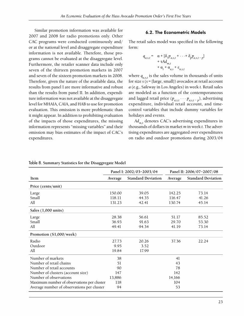
An Economic Evaluation of the Hass Avocado Promotion Order’s First Five Years
23
Similar promotion information was available for 2007 and 2008 for radio promotions only. Other CAC programs were conducted continuously and/or at the national level and disaggregate expenditure information is not available. Therefore, those pro-grams cannot be evaluated at the disaggregate level. Furthermore, the retailer scanner data include only seven of the thirteen promotion markets in 2007 and seven of the sixteen promotion markets in 2008. Therefore, given the nature of the available data, the results from panel I are more informative and robust than the results from panel II. In addition, expendi-ture information was not available at the disaggregate level for MHAIA, CAIA, and HAB to use for promotion evaluation. This omission is more problematic than it might appear. In addition to prohibiting evaluation of the impacts of those expenditures, the missing information represents “missing variables” and their omission may bias estimates of the impact of CAC’s expenditures.
6.2. The Econometric Models
The retail sales model was specifi ed in the following form:
qa,s,t = α + [δ1pa,s,t + . . .+ δppa,s,t – p] + τAdm,t + αt + αa,s + εa,s,t
where qa,s,t is the sales volume in thousands of units for size s (s = {large, small}) avocados at retail account a (e.g., Safeway in Los Angeles) in week t. Retail sales are modeled as a function of the contemporaneous and lagged retail price (pa,s,t
. . . pa,s,t – p), advertising expenditure, individual retail account, and time-control variables that include dummy variables for holidays and events.
Adm,t denotes CAC’s advertising expenditures in thousands of dollars in market m in week t. The adver-tising expenditures are aggregated over expenditures on radio and outdoor promotions during 2003/04
Table 8. Summary Statistics for the Disaggregate Model
Panel I: 2002/03–2003/04 Panel II: 2006/07–2007/08
Item Average Standard Deviation Average Standard Deviation
Price (cents/unit)
Large 150.00 39.05 142.25 73.14Small 118.11 44.35 116.47 41.26All 131.23 42.41 130.74 45.14
Sales (1,000 units)
Large 28.38 56.61 51.17 85.52Small 36.93 91.63 29.70 53.30All 49.41 94.34 41.19 73.14
Promotion ($1,000/week)
Radio 27.73 20.26 37.36 22.24Outdoor 9.95 3.52All 19.84 17.99
Number of markets 38 41Number of retail chains 51 43Number of retail accounts 90 78Number of clusters (account size) 147 142Number of observations 13,886 14,166Maximum number of observations per cluster 118 104Average number of observations per cluster 94 53

Giannini Foundation Research Report 351
24
but include only expenditures on radio promotions during 2007/08. Alternatively, expenditures on radio and outdoor promotions can be introduced as separate explanatory variables in Panel I to estimate differential promotion effects for different media types on avocado demand.
Advertising may have a dynamic effect on demand, increasing sales in the current period and into the future. Such effects may be captured by specifying a distributed lag structure for advertising expenditures (Erdem and Keane 1996; Ackerberg 2001, 2003). How-ever, the nature of CAC’s promotions made it diffi cult to apply such models because the weekly expenditure in each treatment market during the promotion peri-ods was essentially constant. As a result, the data do not provide suffi cient variations between periods to estimate a distributed lag structure.
We fi rst present a framework for program evalua-tion based on a binary treatment variable (the presence or absence of a promotion campaign) and then extend this method to the amount of promotion expenditure, which is a continuous treatment variable. When the promotion variable is binary (i.e., advertising is pres-ent in the market (D = 1) or is absent (D = 0)), the approach of Difference in Difference (DID) is used. The fact that CAC selected a subset of markets for its promotion programs from among the total group on which scanner data were available enables us to construct both treatment and control groups for the program evaluation. The DID approach estimates counterfactual outcomes for the retail accounts in the selected markets that were exposed to CAC’s promo-tion programs. The DID framework for identifying the “treatment effects” of CAC’s promotions on retail sales can be presented by the following linear model:
q(a,t) = δ(t) + η(a) + ψD(a,t) + υ(a,t)
where q(a,t) denotes retail sales of avocados at retail account a at time t. Let the pretreatment period, t = 0, be the period when there was no promotion and let
the treatment period, t = 1, be the period when CAC conducted its promotions. D(a,t) denotes whether or not a retail account was exposed to CAC’s promo-tions at time t. Suppose that only q(a,t) and D(a,t) are observed. We refer to retail accounts that were exposed to CAC’s promotion programs (when D(a,1) = 1) as “treated” and those that were not exposed to the promotions (when D(a,1) = 0) as “controls.” The term D(a,0) equals zero for both the treated and the control group because there was no promotion at t = 0. The coeffi cient ψ represents the treatment effect of CAC’s promotion programs, δ(t) denotes the time-specifi c component, η(a) represents the account-specific effects, and υ(a,t) is the individual transitory error term with a zero mean at both t = 0 and t = 1. The advantage of the panel data set is that it enables us to control idiosyncratic characteristics of individual retailers or markets by use of fi xed effects.
Under the assumption that CAC’s selection for treatment is not correlated with the error term,22 we can obtain the difference in expected retail sales with and without CAC’s promotions for the retail accounts in the treated and control markets as:
E[q(a,1)|D(a,1) = 1] – E[q(a,0)|D(a,1) = 1] = E[q(a,1) – q(a,0)|D(a,1) = 1] = [δ(1) – δ(0)] + [η(a) – η(a)] + ψ[D(a,1) – D(a,0)] = δ(1) – δ(0) + ψ
E[q(a,1)|D(a,1) = 0] – E[q(a,0)|D(a,1) = 0] = E[q(a,1) – p(a,0)|D(a,1) = 0] = [δ(1) – δ(0)] + [η(a) – η(a)] = δ(1) – δ(0).
Notice that the use of a simple comparison of retail sales before and after promotion to evaluate the promotion effect is likely to be biased by tem-poral trends in retail sales or by factors other than the promotion that occurred during both periods. They are represented in the preceding equations by the term δ(1) – δ(0). The DID approach is applied to
22 The set of markets selected for promotion by CAC and HAB have been quite stable since 1997. They represent cities with large market shares for avocado sales and are located in states in which importation of Mexican avocados had been prohibited historically. Thus, market selection is affected by market-specifi c characteristics that do not change during the study period and is not correlated with the individual transitory error term. The market-specifi c characteristics, therefore, can be controlled by fi xed effects.
An Economic Evaluation of the Hass Avocado Promotion Order’s First Five Years
25
construct a counterfactual against which to measure the promotion effect. Therefore, the treatment effect of CAC’s promotion, ψ, can be identifi ed in the following form:
ψ = {E[q(a,1)|D(a,1) = 1] – E[q(a,0)|D(a,1) = 1]} – {E[q(a,1)|D(a,1) = 0] – E[q(a,0)|D(a,1) = 0]}.
Our approach is to measure the promotion vari-able as a continuous variable consisting of the weekly promotion expenditure for each promotion market. In this case, the before-treatment level is represented by the mean level of retail sales and the after-treatment level is represented by deviation of sales from the mean level. The estimated coeffi cient of the promo-tion variable presents the treatment effect of CAC’s promotions—that is, the difference in deviations of retail sales from individual means between promo-tion and nonpromotion markets. The comparison of retail sales between promotion and nonpromotion markets is made by holding average retail sales at the individual retail account level constant. The promo-tion effects, therefore, can be estimated by a “within” model. The evaluation of promotion effects, then, is based on deviations at the individual chain level. However, average retail sales in promotion markets may also increase as a result of CAC’s promotions. We can estimate the effects of the promotion program on average retail sales using a “between effects” model that compares sales in promotion and nonpromotion markets.
In the following, we present results from four econometric models: a pooled model, a within model, a between-effects model, and a random-effects model. The pooled and random-effects models utilize varia-tions over time and in cross-section. The between-effects model uses only variations between individual chains
in cross-section. The within model uses deviations over time for the dependent and explanatory variables from their time-averaged values.
6.3. Results
We provide a brief discussion of the overall results for the within model, which are summarized in Table 9. Tables 10 and 11 focus specifi cally on promotion impacts estimated across several econometric models. The seasonal patterns of retail demand for avocados were quite stable over the study period. Avocado demand did not vary signifi cantly during the same month or the same holiday/event across different years. The estimates for the year indicator or dummy variables show that retail sales grew steadily over the years, a determination that is consistent with results from the aggregate model. Retail sales were greatest during the months of May, June, and July and then began to decline in August or September.
Retail demand for avocados is signifi cantly greater during particular holidays and events. Super Bowl Sunday generated the most sales, followed by Cinco de Mayo, Christmas/New Year’s Day, Independence Day, and Labor Day. Retail sales grew signifi cantly over time for Cinco de Mayo with sales growth more than doubling in 2007 and 2008 during that week compared to 2003 and 2004.23
The results indicate that retail demand for avocados at the individual chain level is price elastic. The estimated elasticities are –2.034 during 2003/04 and –2.238 during 2007/08.24 Lagged retail prices had signifi cant and positive effects on retail sales in the current period.25 However, retail sales responded mainly to changes in the contemporaneous retail price.
23 Li (2007) demonstrates that retail prices and margins were signifi cantly lower during some holidays/events associated with high demand for avocados (e.g., Christmas/New Year’s Day, Super Bowl Sunday, and Cinco de Mayo), indicating that retailers are using avocados as sale items during these periods of peak demand, thereby further stimulating demand.24 Note that demand at the level of the individual retail chain is expected to be much more elastic than demand at the market level. High price elasticity at the chain level refl ects competition between chains for price-conscious consumers and also the response of both store-loyal consumers and price-conscious consumers to price promotions for avocados. In essence, these estimated elasticities demonstrate that avocados are a product that responds well to price promotions. Due to their perishable nature, they are an effective product for promotions in a second dimension because they cannot be stockpiled by consumers.25 This result is also intuitive. Even though avocados are perishable, the estimated impact of lagged prices shows that people are willing and able to defer purchases in period t – 1, for example, if prices are high in hopes of obtaining a better price in period t.

Giannini Foundation Research Report 351
26
Table 9. Estimation Results for the Retail Sales Model: Within Model
Dependent Variable: Retail Sales (1,000 units)
Panel I: 2003/04 Panel II: 2007/08
Coeffi cient Standard Error Coeffi cient Standard Error
Price (cents/unit) t –0.508*** (0.088) –0.736*** (0.123) t − 1 0.155*** (0.042) 0.252*** (0.096) t − 2 0.135*** (0.024) 0.096*** (0.043)
Price elasticity at means t –2.034 (0.126) –2.238 (0.140) t − 1 1.621 (0.028) 0.764 (0.085) t − 2 0.540 (0.009) 0.291 (0.017)
Promotion ($1,000) 0.014 (0.060) –0.139 (0.080)
Christmas /New Year 7.06*** (1.82) 6.17*** (1.30)Super Bowl 17.59*** (3.86) 15.94*** (4.52)Valentine’s/Presidents’ Day 0.73 (1.21) –0.43 (2.10)Oscar Awards 1.29 (1.25) –4.53* (2.33)Cinco de Mayo 4.52** (2.11) 11.12*** (4.03)Easter 1.52 (1.40) –0.74 (1.22)Mothers’ Day –1.20 (1.50) –0.44 (1.87)Memorial Day 2.70* (1.45) –1.14 (2.03)Fathers’ Day –3.52 (3.24) 0.61 (1.87)Independence Day 4.11*** (1.35) 5.12*** (1.36)Labor Day 5.19*** (1.70) 2.32*** (0.88)Thanksgiving –1.51 (2.93) –7.42*** (1.88)
2002 (base) 0.0 0.02003 0.97 (1.41)2004 4.78** (2.25)
2007 (base) 0.0 0.02008 2.88 (2.15)
January –1.53 (1.18) –0.59 (2.01) February –1.60 (1.34) 3.30 (2.67) March –0.64 (1.44) 3.69* (1.95)April –0.29 (1.50) 1.71 (1.82)May 3.68*** (1.39) 8.62*** (2.73)June 7.74** (3.16) 5.26** (2.30)July 0.00 (1.41) 6.34*** (2.01)August 1.17 (1.50) 3.85** (1.49)September 4.34*** (1.63) 0.06 (1.12)November 1.57 (1.75) –0.45 (1.68)December –1.21 (1.75) –6.10*** (1.50)Constant –4.11*** (1.35) 90.06 (9.78)
R2 0.108 0.062Number of observations 15,360 13,838Maximum no. of observations per cluster 118 104Number of clusters 147 142
Note: Asterisks denote statistical signifi cance levels with one, two, and three stars denoting statistical signifi cance at 90%, 95%, and 99%, respectively.

An Economic Evaluation of the Hass Avocado Promotion Order’s First Five Years
27
An alternative model framework included lags of retail sales of a variety of lengths but the lagged sales had no important effects either in terms of magnitude or statistical signifi cance. These results indicate the absence of state dependence in weekly retail sales of avocados, or the absence of a consumption habit effect for avocados, as measured on a weekly basis.26
Turning now to promotion, the measured impact of CAC’s promotion program on retail sales for avocados is comprised of two effects. First, CAC’s promotion may contribute to higher average retail sales in pro-motion markets relative to nonpromotion markets. However, the estimated coeffi cient of the promotion variable from the between-effects model consists of both the effect of promotion and the effect of other unobserved factors on average retail sales. These unobserved factors, which may contribute to differ-ences in average retail sales between promotion and nonpromotion markets, need to be controlled to attain clean identifi cation of the effect of promotion.
Second, the effect of the promotion program on retail sales is measured by how much retail sales deviate from mean levels as the promotion expen-diture increases or as the promotion program is conducted in a week. This effect is estimated by the within model by controlling the difference in average retail sales between promotion and nonpro-motion markets. Clearly, the overall promotion effect includes both the effect on average retail sales and the effect on deviations of retail sales from the aver-age in promotion markets. Both the pooled and the random-effects models utilize variations in promotion both in cross-section and over time to estimate the overall promotion effect. The random-effects model is preferred to the pooled model in the presence of unobserved heterogeneity. Nevertheless, both provide valuable information.
Tables 10 and 11 present the estimated effects of promotion on retail sales by the pooled, between-effects, within, and random-effects models for the data in Panel I and Panel II, respectively. Estimation I, which
is reported in the top portion of each table, does not control unobserved factors that may contribute to the difference in average retail sales between promotion and nonpromotion markets. As a result, the estimated promotion effect from the pooled, between-effects, and random-effects models could be biased. Estima-tion II introduces a dummy variable to control the difference in average retail sales between promotion and nonpromotion markets in the pooled, between-effects, and random-effects models. Estimation III uses dummy variables for individual promotion markets to control differences in average retail sales between each promotion and nonpromotion market.27
Consider fi rst the estimates from Panel I, which are shown in Table 10. The estimated promotion effects from the between-effects model show that average weekly retail sales for each size of avocado at retail accounts were 1,472 units greater in promo-tion markets than in nonpromotion markets for each $1,000 of weekly promotion expenditure (estimation III). The average weekly promotion expenditure was $20,419 in a promotion market. Therefore, average weekly retail sales increased by an estimated 30,057 units for each size of avocado sold at retail accounts in promotion markets. Introducing dummy variables to control unobserved factors that may contribute to differences in average retail sales between promotion and nonpromotion markets reduces the size of the estimated promotion effect signifi cantly (compare the promotion coeffi cients in estimation I versus esti-mation III). The introduction of additional variables decreases effi ciency in the estimations and increases standard errors. The increase in average retail sales in promotion markets due to promotion is positive but is not statistically signifi cant for estimations II and III.
Second, the results from the within model indicate that sales at a retail account in a promotion market increased slightly as promotion expenditure increased during promotion periods but the effect was not statistically signifi cant.
26 The other rationale to include lagged retail sales in the model is that serial correlation may exist in retail sales. If that is the case, excluding the lagged retail sales could generate omitted variable bias. This did not appear to be an issue for the estimation. The post-estimation tests show that residuals are not serially correlated and overidentifi cation tests show that the set of variables is exogenous.27 In other words, estimation III contains a separate {0,1} indicator variable to identify market-specifi c effects on sales (see the bottom portion of Table 10).

Giannini Foundation Research Report 351
28
Table 10. The Effects of Promotion on Retail Sales from Panel I: 2003/04
Pooled Between Within Random Effects
Estimate Std Error Estimate Std Error Estimate Std Error Estimate Std Error
Estimation I
Retail price t –0.654*** 0.128 –0.701*** 0.180 –0.508*** 0.088 –0.509*** 0.088
t − 1 0.092* 0.052 0.155*** 0.042 0.154*** 0.042
t − 2 –0.003 0.064 0.135*** 0.024 0.134*** 0.024
Promotion expenditure 0.792** 0.322 2.741*** 1.107 0.014 0.060 0.017 0.060
Small size –9.959 7.786 –15.059 12.019 –1.077 10.675
R2 0.115 0.167 0.108 0.072Root mean square error 72.811 63.634 32.482 32.482Intraclass correlation 0.803Λ 0.000 1.000 0.954
Estimation II
Retail price t –0.621*** 0.116 –0.659*** 0.181 –0.509*** 0.088
t −1 0.102** 0.051 0.155*** 0.042
t −2 0.036 0.056 0.134*** 0.024
Promotion expenditure 0.059 0.386 0.288 1.806 0.014*** 0.060
Promotion market 36.510*** 12.019 31.060* 18.128 39.006*** 11.671
Small size –9.245 7.760 –14.782 11.940 –2.000*** 10.087
R2 0.158 0.184 0.141Root mean square error 71.016 63.208 32.482Intraclass correlation 0.801Λ 0.000 0.954
Estimation III
Retail price t –0.591*** 0.102 –0.581*** 0.170 –0.509*** 0.088
t − 1 0.116** 0.048 0.155*** 0.042
t − 2 0.065 0.045 0.134*** 0.024
Promotion expenditure 0.035 0.069 1.472 3.701 0.014 0.060
Promotion market
Phoenix 16.951 13.343 5.825 26.913 21.829* 12.018
Los Angeles 69.981*** 25.560 39.899 67.035 73.630*** 25.476
San Francisco 39.372* 23.723 25.232 39.694 40.201* 23.523
Atlanta –7.070 8.219 –27.905 53.288 –2.742 6.531
Portland 2.226 8.329 –2.324 29.755 3.070 7.553
Dallas 4.710 9.940 –10.090 28.089 9.278 9.572
Houston 48.944* 28.158 35.689 28.709 54.332* 30.497
San Antonio 289.623 196.875 280.932*** 38.019 296.148 201.896
Small size –4.831 7.487 –10.423 10.421 –0.834 8.631
R2 0.364 0.433 0.355RMSE 61.763 54.025 32.482Intraclass correlation 0.748Λ 0.000 0.946
Note: Asterisks denote statistical signifi cance levels with one, two, and three stars denoting statistical signifi cance at 90%, 95%, and 99%, respectively.

An Economic Evaluation of the Hass Avocado Promotion Order’s First Five Years
29
Table 11. The Effects of Promotion on Retail Sales from Panel II: 2007/08
Pooled Between Within Random Effects
Estimate Std Error Estimate Std Error Estimate Std Error Estimate Std Error
Estimation I
Retail price t –0.759*** 0.121 –0.272** 0.134 –0.736*** 0.123 –0.736*** 0.122
t − 1 0.245** 0.097 0.252*** 0.096 0.252*** 0.096
t − 2 0.083 0.058 0.096** 0.043 0.096** 0.043
Radio expenditure 1.130*** 0.278 16.419*** 2.167 –0.139 0.080 –0.134* 0.080
Small size –30.349*** 11.080 –25.143*** 9.686 –29.703*** 10.967
R2 0.117 0.350 0.193 0.100Root mean square error 69.867 53.523 31.489 31.706Intraclass correlation 0.743Λ 0.000 1.000 0.942
Estimation II
Retail price t –0.745*** 0.117 –0.274** 0.136 –0.736*** 0.122
t −1 0.254** 0.100 0.252*** 0.096
t −2 0.099* 0.058 0.096** 0.043
Radio expenditure 0.352** 0.176 16.169*** 3.608 –0.134* 0.080
Radio promotion market 55.327*** 12.019 1.378 16.013 –0.405 13.922
Small size –29.911*** 7.760 –25.206** 9.749 –29.705 10.984
R2 0.236 0.350 0.098Root mean square error 64.991 53.716 31.646Intraclass correlation 0.744Λ 0.000 0.942
Estimation III
Retail price t –0.685*** 0.102 –0.174 0.123 –0.735*** 0.088
t − 1 0.290*** 0.048 0.252*** 0.042
t − 2 0.163*** 0.045 0.097** 0.024
Radio expenditure –0.140 0.069 –22.684 36.705 –0.136* 0.060
Radio market
Phoenix 49.559*** 17.283 93.606 71.562 50.197*** 15.955
Los Angeles 118.715*** 30.768 298.736 291.426 115.488*** 31.392
San Francisco 191.403*** 54.709 290.859* 160.341 187.585*** 55.119
Atlanta 4.303 16.164 126.789 185.952 –6.675 14.974
Portland 15.702 13.438 40.357 50.450 20.182* 11.263
Dallas 3.562 5.363 74.942 116.306 2.980 5.025
Houston 45.722** 23.012 116.805 115.186 44.471** 30.497
Seattle 17.154 15.017 51.899 62.819 22.606 14.211
Small size –22.650*** 7.558 –21.489** 8.559 –26.449*** 8.220
R2 0.454 0.532 0.448RMSE 54.987 46.773 31.646Intraclass correlation 0.687Λ 0.000 0.933
Note: Asterisks denote statistical signifi cance levels with one, two, and three stars denoting statistical signifi cance at 90%, 95%, and 99%, respectively.

Giannini Foundation Research Report 351
30
Third, the estimated promotion effects from the random-effects model were the same as those from the within model after effects of individual promotion markets were controlled in estimation II and III. This suggests that promotion on the whole increased aver-age retail sales for promotion markets over those in nonpromotion markets. Promotion effects from week to week in each promotion market were small. This is likely due to the promotion effects merging over time, increasing average retail sales as a whole. Therefore, the majority of the promotion effect was identifi ed via the between-effects model rather than by the within model.28 This conclusion is consistent with the results of Erdem and Keane (1996), who were able to apply a distributed lag structure to discern the impact of advertising on detergent sales and concluded that advertising had weak short-run effects but a strong cumulative effect in the long run.
Table 11 presents the estimation results from Panel II (2007/08). First, the estimated promotion effects (estimation II) from the between-effects model show that average weekly retail sales for each size of avocado at retail accounts in promotion markets were 16,169 units greater than those in nonpromotion markets for each $1,000 of average weekly promotion expenditure. The estimated impact of these radio promotions is eleven times greater than the estimated impact of CAC’s promotion program (which included both radio and outdoor promotion) during the 2002/03–2003/04 crop years. The average weekly promotion expenditure was $37,360 in a promotion market. Therefore, average weekly retail sales increased by an estimated 604,474 units for each size of avocado sold at retail accounts in promotion markets.
Estimation II controls unobserved factors that may contribute to differences in average retail sales between promotion and nonpromotion markets. The results show that the difference was primarily and signifi cantly explained by the difference in average retail sales due to promotion. These results are differ-ent from those for 2003/04 (Table 10), which show that the estimated promotion effects were reduced signifi cantly after controlling the unobserved factors
that may account for differences in average sales between promotion and nonpromotion markets.
Estimation III includes dummy variables for each promotion market in the data to control differences in average retail sales between promotion markets. The estimated coeffi cient for the radio promotion expen-diture is negative and not statistically signifi cant in estimation III. This is mostly due to inevitable multi-collinearity problems because (1) the radio promotion expenditure is highly collinear with the set of dummy variables for promotion markets and (2) introduction of additional variables decreases estimation effi ciency. Nonetheless, the estimated coeffi cients for promotion markets provide valuable information by identifying the markets in which average retail sales were signifi -cantly higher. Note that the estimates may represent some effect of radio programs because the promotion variable is highly correlated with the dummy variables for promotion markets. The estimates also may rep-resent the effect of other promotion programs that are not included in the model due to lack of available data. The coeffi cient estimates for individual promo-tion markets are markedly higher for 2007/08 than for 2003/04. The markets associated with the highest average sales in 2007/08 were Los Angeles, Atlanta, San Francisco, Houston, and Phoenix while the high-est sales in 2003/04 were San Antonio (data were not available for San Antonio during 2007/08), Los Angeles, Houston, and San Francisco.
Second, the results from the within and random-effects models indicate that radio promotions had an insignifi cant effect on retail sales during the promo-tion periods both in terms of the magnitude of the estimated effects and their statistical signifi cance. This may be because the effects of individual radio promotions were consolidated over time and increased average sales in the overall market and/or because the effects of radio programs were blended with the effects of other promotion programs that were conducted but are omitted from the estimation (due to lack of avail-able data), such as programs that were conducted in the treatment cities during 2007/08 by CAIA, MHAIA, and/or HAB.
28 In results not reported here but available from the authors upon request, we investigated decomposing the impact of CAC’s expenditures by media type—radio advertising versus outdoor advertising. Results suggest a greater effectiveness for radio pro-motions relative to outdoor advertising but the effects were not statistically signifi cant.

An Economic Evaluation of the Hass Avocado Promotion Order’s First Five Years
31
Taken together, the results suggest that radio promotion signifi cantly increased average retail sales in promotion markets compared with average retail sales in nonpromotion markets. The estimated promo-tion effects in 2007/08 are also markedly higher than the promotion effects during 2003/04.
The various models reported in Tables 10 and 11 estimated promotion effects from different perspectives but the most relevant results are those for estimation II from the between-effects model. Those effects are comprised of two elements: a signifi cant increase in sales during the promotion period (the wave) and a sales increase stretched during and beyond the pro-motion period (level). The results from panels I and II consistently indicate that the second effect (increase in the average level) dominates. The fi rst effect, mea-sured by the within and random-effects models, is small because (1) promotion expenditures did not vary much from week to week and/or (2) because the effects of promotion were carried over time and, hence, the promotion effects were consolidated to increase average retail sales (the average level).
A comparison of the results from estimations I and II suggests that the heterogeneity between promotion and nonpromotion markets needs to be controlled and, hence, that estimation II is preferable to estimation I. The results from estimation III must be viewed with some caution due to the problem of multicollinearity. The value of estimation III is the resulting ability to see comparative or relative promotion effects between markets and between two panel periods rather than having to observe only absolute estimates.
6.4. The Effects of the California Avocado Commission’s Promotions on Retail
and Shipping-Point Prices
The fi ndings for retail sales for avocados suggest, on balance, that CAC’s promotion program had a posi-tive effect on retail sales for avocados. We now seek to determine the impacts, if any, of the program on retail prices and prices at the shipping point. This analysis is conducted only on Panel I during 2003/04 because expenditure data were not available for both radio and outdoor programs during 2007/08.
Table 12 presents the estimated effects of CAC’s promotion program on the retail and shipping-point price for avocados. Both models use weekly dummy variables as time-control variables. Panel 1 in Table 12 contains the estimated impact of incremental $1,000 expenditures by CAC in the targeted market while panel 2 estimates the cumulative impact in terms of total expenditure during each of the promotion periods.
If arbitrage at the shipping level is effi cient between promotion and nonpromotion markets and between promotion and nonpromotion weeks or periods, CAC’s promotion program should have no signifi cant effect on shipping-point (FOB) prices to alternative destination markets. Successful promotions in tar-geted markets increase demand in those markets, which should cause shippers to expand shipments to those markets relative to nonpromotion markets. This reallocation of supply between markets should continue until the shipping-point prices to all desti-nation markets are equated if arbitrage by shippers is effi cient. A similar argument applies to intertem-poral arbitrage designed to have shipments in place at destination markets to coincide with promotion periods. The results for the shipping-point price of avocados shown in Table 12 reveal a small positive estimated impact of promotion on prices to target markets. Shipping-point prices to promotion mar-kets during promotion periods were 0.116¢ per unit higher (panel 2) than shipping-point prices during nonpromotion periods and to nonpromotion markets. However, this estimated impact is not statistically signifi cant for either radio or outdoor promotion by CAC, which is consistent with the effi cient arbitrage hypothesis.
A possible concern for industry generic promotion relates to retailer responses to promotions. Successful promotions targeted to consumers increase demand for avocados. That increase in demand can be refl ected in increased retail sales, higher retail prices, or a com-bination of both. To the extent that retailers increase prices and margins to capture the higher demand generated by industry promotions, their actions vitiate the effectiveness of the programs from the industry’s perspective. The increase in sales that is necessary to

Giannini Foundation Research Report 351
32
increase the price received by growers and shippers will not occur. Conversely, if retailers did not capture the benefi ts of increases in demand for avocados due to CAC’s promotion program through higher prices, we would expect the benefi t to accrue at the grower-shipper level in the form of higher FOB prices.
An interesting possibility supported by some research is that retailers may reduce retail prices in response to a positive demand shock for a product, most likely as a way to entice customers to the store to then purchase additional items. Evidence of lower retail prices for avocados in response to CAC’s promo-tion program would mean that retailers’ actions are
reinforcing (instead of offsetting) the impacts of CAC’s promotion. The results in Table 12 show that retail prices during promotions were 0.363¢ (0.405¢) per unit lower than retail prices in nonpromotion periods and in nonpromotion markets in 2003 (2004). But the effect is not statistically signifi cant due to the insignifi -cance of the promotion coeffi cient.29 Thus, there is no evidence that retailers capture some of the demand expansion induced by CAC promotion through higher retail prices and some very weak evidence that they may contribute to the effectiveness of the program by lowering prices to support industry promotions.
Table 12. The Effects of California Avocado Commission Promotions on Retail Price and Shipping-Point Price
1. Estimation Results
Retail Price (cents/unit, weekly)
Shipping-Point Price(cents/unit, weekly)
Estimate Standard Error Estimate Standard Error
Promotion (pooled) –0.019 0.020 0.006 0.024
Radio –0.019 0.021 0.028 0.018
Outdoor –0.023 0.079 0.083 0.062
2. The Estimated Effects of CAC’s Promotion during 2003/04
Retail Price (cents/unit, weekly)
Shipping-Point Price(cents/unit, weekly)
2003 2004 2003 2004
Radio Radio 1 –0.369 –0.396 0.553 0.592
Radio 2 –0.396 –0.402 0.593 0.602
Radio 3 –0.382 –0.387 0.571 0.579
Radio 4 –0.240 –0.364 0.359 0.545
Average –0.347 –0.387 0.519 0.580
Average
Radio –0.275 –0.303 0.147 0.161
Outdoor –0.159 –0.167 0.085 0.089
Promotion –0.363 –0.405 0.116 0.130
Note: Asterisks denote statistical signifi cance levels with one, two, and three stars denoting statistical signifi cance at 90%, 95%, and 99%, respectively.
29 These effects are found by multiplying the estimated coeffi cient on pooled promotion contained in the top half of the table by the mean promotional expenditure in the targeted markets.

An Economic Evaluation of the Hass Avocado Promotion Order’s First Five Years
33
7. EVALUATION OF THE HASS AVOCADO BOARD’S NETWORK MARKETING CENTER PROGRAM
HAB conducts an active internet information program through its Network Marketing Center to share information to promote
orderly marketing. As stated in its fi rst annual report (2003):
The primary goal behind the INFOTECH plank of HAB’s Strategy is to develop “Stra-tegic Intelligence” that will enable avocado marketers to share information essential to orderly marketing throughout the full 12-month season and ameliorate seasonal transition points and concomitant market instability between sources. This initiative is designed to help ALL sellers in the U.S. market develop a much-needed framework to ensure orderly fl ow of fruit and market stability. The benefi ts from such an end state would inure to consumers, supermarket retailers and those suppliers selling Hass avocados in the U.S. (p. 11–12)
All participants in the Hass avocado marketing chain have access to the HAB website (AvoHQ.com) where they are able to share harvest and shipment planning information. The 2006/07 annual report (page 3) indi-cates that HAB’s technology infrastructure supported more than 2,500 users and use has continued to grow since then. This ongoing information exchange is intended to smooth shipments to major U.S. markets, prevent surplus and shortage situations, and promote stable FOB and retail pricing.
7.1. Variability of Prices and Quantities over Time
Empirical evaluation of the benefi ts of an information program is diffi cult and the activities of HAB are no exception. We can, however, examine some industry statistics related to HAB’s goal of an orderly fl ow of fruit and market stability that provide an indication of progress toward meeting program goals. We mea-sure the variability of prices and quantities over time using the standard deviation of weekly prices and quantities for California and imported avocados. We
fi rst examined the standard deviation of California FOB avocado prices for the most recent ten-year period (1998–2007). While there was not an evident trend over time, the weekly standard deviation of the FOB price for the most recent fi ve years averaged 0.2045 while the same average for the fi rst fi ve years was 0.2843. At the same time, the weekly standard deviation of California shipments increased from an annual average of 2,293,841 pounds for the fi rst fi ve years (1998–2002) to 4,303,944 pounds for the most recent fi ve years (2003–2007). This indicates that, while the size of California shipments has become more variable, efforts to coordinate imports with Cali-fornia shipments have smoothed total weekly avocado shipments and prices during the marketing year. The most recent fi ve-year comparison of California ship-ments with total weekly shipments (California plus imports) is shown in Table 13. While rising imports have the potential to introduce additional quantities and price variability into the U.S. market, the opposite has occurred. Imports have been timed to maintain a rather steady fl ow of avocados to retail markets, which tends to stabilize prices at both the FOB and the retail level. A portion of the smoothing of quantities and prices despite signifi cantly increased imports can and should be attributed to the active HAB informa-tion program.
Previous research on specialty agricultural com-modities has demonstrated that decreased price variability can benefi t both producers and consumers.
Table 13. Standard Deviation of Weekly California and Total Avocado Shipments, 2003–2007
Total: California Year California Plus Imports
2003 3,359,560 1,479,939
2004 5,020,240 2,693,992
2005 4,593,614 2,052,438
2006 6,399,061 3,330,162
2007 3,483,128 1,990,026
Five-year average 4,303,944 2,309,312

Giannini Foundation Research Report 351
34
Market conditions present in the U.S. avocado indus-try that can lead to this result are: (1) food retailers that have market power in setting their retail prices, (2) a perishable product, and (3) retail chains that purchase the product directly from grower-shippers with operations that are small relative to the chain buyers. Under these conditions, buyers can use large or temporarily large supplies to bid down shipping-point prices and increase their margins (Sexton and Zhang 1996). These same conditions can also lead to asymmetric price transmission from the producer to the retail level as evidenced by retail prices responding more quickly and more fully to FOB price increases than to FOB price decreases.30
Li (2007) analyzed the price transmission process for avocados for increases and decreases in shipping-point prices. She summarized the results of her extensive analysis of asymmetric price adjustments for California avocados as follows:
The [retail] price adjustment rates were 76% to an increase in shipping price and 29% to a decrease in shipping price, and the adjustment was made slower in response to an increase in shipping price than to a decrease in shipping price. Asymmetry in price adjustment to changes in shipping price suggests that retail-ers were able to manipulate price adjustments to increases and decreases in shipping price to attain higher profi ts. (p. 333)
Thus, retail prices for avocados respond more fully to shipping-point price increases than to shipping-point price decreases. As a result, retail price margins for avocados tend to increase with larger and more frequent price changes or decrease with smaller and less frequent price changes. Price instability promotes higher retailer margins at the expense of both produc-ers and consumers while increased price stability tends to decrease annual average retailer margins with benefi ts fl owing to both producers and consumers. Thus, information programs that smooth the fl ow of avocados to U.S. markets and the price of those avo-cados benefi t both producers and consumers.
7.2. Costs of the Hass Avocado Board’s Information Program
The annual costs of HAB’s information program are listed by category in each HAB annual report (2003–2007) and are summarized in Table 14. Annual expenditures for the information program ranged from $340,179 to $1,090,228 over fi ve years with an average annual cost of just under $750,000. Total fi ve-year costs for the categories of information, analysis, and the Network Marketing Center fell in a rather tight range of $530,514 to $536,936. Almost 57% of the total cost for the fi rst fi ve years ($2,125,915) was in the interaction category.
Table 14. Annual and Total Costs of the Hass Avocado Board’s Information Programs by Cost Category, 2003–2007
Year
Cost Category 2003 2004 2005 2006 2007 Grand Total
Information $28,619 $219,553 $71,104 $123,434 $94,226 $536,936
Analysis $0 $44,843 $168,976 $197,375 $120,281 $531,475
Interaction $286,560 $658,956 $378,566 $404,241 $397,592 $2,125,915
Network marketing center $0 $166,876 $66,163 $179,052 $118,423 $530,514
Total information $340,179 $1,090,228 $684,809 $904,102 $730,522 $3,749,840
Source: Hass Avocado Board annual reports, 2003–2007.
30 Studies that have found asymmetry in price transmission for food products include Kinnucan and Forker (1987) for dairy products; Pick, Karrenbrock, and Carman (1990) for citrus; Zhang, Fletcher and Carley (1995) for peanuts; and Carman and Sexton (2005) for fl uid milk in the western United States.
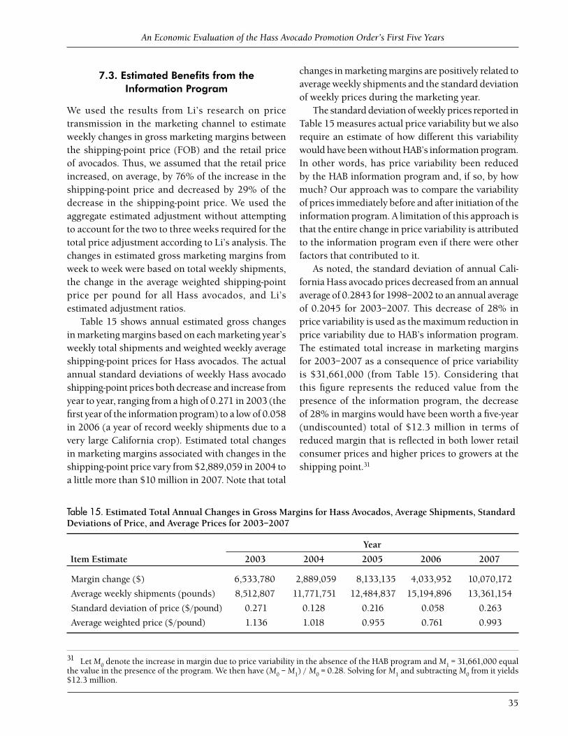
An Economic Evaluation of the Hass Avocado Promotion Order’s First Five Years
35
7.3. Estimated Benefits from theInformation Program
We used the results from Li’s research on price transmission in the marketing channel to estimate weekly changes in gross marketing margins between the shipping-point price (FOB) and the retail price of avocados. Thus, we assumed that the retail price increased, on average, by 76% of the increase in the shipping-point price and decreased by 29% of the decrease in the shipping-point price. We used the aggregate estimated adjustment without attempting to account for the two to three weeks required for the total price adjustment according to Li’s analysis. The changes in estimated gross marketing margins from week to week were based on total weekly shipments, the change in the average weighted shipping-point price per pound for all Hass avocados, and Li’s estimated adjustment ratios.
Table 15 shows annual estimated gross changes in marketing margins based on each marketing year’s weekly total shipments and weighted weekly average shipping-point prices for Hass avocados. The actual annual standard deviations of weekly Hass avocado shipping-point prices both decrease and increase from year to year, ranging from a high of 0.271 in 2003 (the fi rst year of the information program) to a low of 0.058 in 2006 (a year of record weekly shipments due to a very large California crop). Estimated total changes in marketing margins associated with changes in the shipping-point price vary from $2,889,059 in 2004 to a little more than $10 million in 2007. Note that total
changes in marketing margins are positively related to average weekly shipments and the standard deviation of weekly prices during the marketing year.
The standard deviation of weekly prices reported in Table 15 measures actual price variability but we also require an estimate of how different this variability would have been without HAB’s information program. In other words, has price variability been reduced by the HAB information program and, if so, by how much? Our approach was to compare the variability of prices immediately before and after initiation of the information program. A limitation of this approach is that the entire change in price variability is attributed to the information program even if there were other factors that contributed to it.
As noted, the standard deviation of annual Cali-fornia Hass avocado prices decreased from an annual average of 0.2843 for 1998–2002 to an annual average of 0.2045 for 2003–2007. This decrease of 28% in price variability is used as the maximum reduction in price variability due to HAB’s information program. The estimated total increase in marketing margins for 2003–2007 as a consequence of price variability is $31,661,000 (from Table 15). Considering that this fi gure represents the reduced value from the presence of the information program, the decrease of 28% in margins would have been worth a fi ve-year (undiscounted) total of $12.3 million in terms of reduced margin that is refl ected in both lower retail consumer prices and higher prices to growers at the shipping point.31
Table 15. Estimated Total Annual Changes in Gross Margins for Hass Avocados, Average Shipments, Standard Deviations of Price, and Average Prices for 2003–2007
Year
Item Estimate 2003 2004 2005 2006 2007
Margin change ($) 6,533,780 2,889,059 8,133,135 4,033,952 10,070,172
Average weekly shipments (pounds) 8,512,807 11,771,751 12,484,837 15,194,896 13,361,154
Standard deviation of price ($/pound) 0.271 0.128 0.216 0.058 0.263
Average weighted price ($/pound) 1.136 1.018 0.955 0.761 0.993
31 Let M0 denote the increase in margin due to price variability in the absence of the HAB program and M1 = 31,661,000 equal the value in the presence of the program. We then have (M0 – M1) / M0 = 0.28. Solving for M1 and subtracting M0 from it yields $12.3 million.

Giannini Foundation Research Report 351
36
The division of the total benefi t, as well as the assessment cost to fund the information program, between consumers and producers depends on the value of consumers’ price elasticity of demand, εD, relative to producers’ price elasticity of supply, εS, for avocados to the U.S. market. As noted in section 5, we have good estimates of εD from the econometric analysis in section 4 but lack a reliable method by which to estimate εS in the current market environ-ment. Thus, section 5 reported benefi t-cost ratios for alternative values of εS of 0.5, 1.0, and 2.0. The share of a change in margin going to consumers in terms of lower price is
ΔP = εS .εS – εD
For purposes of this calculation, we computed εD at the average of price and quantity for the past ten years. Although the estimates vary depending on the specifi c econometric model estimated, all produced a value of εD ≈ –0.25 during this period. Thus, the producers’ share of the benefi t and the cost from the information program varies from about 11% to 33% depending on the value assumed for εS. Assuming that the entire margin reduction can be attributed to HAB’s informa-tion program, the total net benefi t is the $12.3 million gross benefi t minus the $3.75 million program cost, resulting in $8.55 million of net benefi t. Producers’ share of this net benefi t is then in the range of $0.94 to $2.82 million dollars with the remainder of the net benefi t going to U.S. avocado consumers.
An Economic Evaluation of the Hass Avocado Promotion Order’s First Five Years
37
8. CONCLUSIONS
This study has focused on the impact of HAB promotion programs on demand for avocados. The estimated elasticity of promotion ranged
from a high of 0.37 to a low of 0.15 depending on model specifi cation. It appears that the trend variables accounted not only for the effects of “tastes and prefer-ences” but also for some of the effects of promotion. Thus, the low estimate of the promotion elasticity is undoubtedly too low and is viewed as conservative.
Simulations of benefi t-cost ratios using the highest and lowest estimated promotion response and supply elasticities of 0.5, 1.0, and 2.0 indicate that producer-funded promotion programs not only expanded demand for avocados but provided a positive return on funds spent. The estimated benefi t-cost ratios range from 1.12 to 6.73. More importantly, each exceeds 1.0, meaning that (1) the promotion programs supported by HAB during its fi rst fi ve years yielded net benefi ts to producers and (2) the programs could have been profi tably expanded during the 2003–2007 period of analysis. Given the range of promotion and supply elasticities used for the simulations, our best estimate of the benefi t-cost ratio for HAB promotion programs is somewhere in the middle of the simulated range of 1.12 to 6.73—most likely, in an interval between 2.5 and 4.0.
The orderly marketing objective of HAB’s informa-tion program implies a smooth matching of weekly supply and demand with stable prices. Both produc-ers and consumers benefi t from price stability when retail prices respond more to FOB price increases than to price decreases as occurs with avocados. A comparison of weekly avocado prices for the fi ve years
preceding the creation of HAB with the fi rst fi ve years of its operation shows that price variability decreased an average of 28%. Estimated total producer and consumer benefi ts from HAB’s information program may have been as much as $12.3 million. Subtracting $3.75 million for program costs leaves a net benefi t of $8.55 million. Producers’ share of this net benefi t is estimated to be in the range of $0.94 to $2.82 million with the remainder of the net benefi t going to U.S. avocado consumers.
Analysis of avocado promotion programs in major retail markets suggests that radio promotion signifi cantly increased average retail sales in promo-tion markets over the same sales in nonpromotion markets. Previous results also suggested that radio is a more effective medium than outdoor advertising but the difference in effect was not statistically signifi cant. The opportunity to conduct an evaluation based on available retail scanner data was limited by the indus-try’s inability to systematically provide disaggregate promotion expenditure information.
A potential problem with producer-funded con-sumer promotion programs is that retailers may respond to increased demand by raising retail prices, thereby curtailing the demand expansion. Analysis of retail pricing behavior for avocados indicates, however, that this does not seem to have occurred sys-tematically and, thus, was not a problem limiting the impact of promotion. Instead, there is weak evidence that retailers may contribute to the effectiveness of the programs by lowering prices to support industry promotions.

Giannini Foundation Research Report 351
38

An Economic Evaluation of the Hass Avocado Promotion Order’s First Five Years
39
REFERENCES
Ackerberg, D.A. “Empirically Distinguishing Informa-tive and Prestige Effects of Advertising.” RAND Journal of Economics 32 (2001):316–333.
Ackerberg, D.A. “Advertising, Learning, and Con-sumer Choice in Experience Good Markets: An Empirical Appraisal.” International Economic Review 44 (2003):1007–1040.
Alston, J.M., J.A. Chalfant, J.E. Christian, E. Meng, and N.E. Piggott. The California Table Grape Commission’s Promotion Program: An Evaluation. Davis CA: Giannini Foundation of Agricultural Economics Monograph 43, 1997.
Alston, J.M., H.F. Carman, J.A. Chalfant, J.M. Crespi, R.J. Sexton, and R.J. Venner. The California Prune Board’s Promotion Program: An Evaluation. Davis CA: Giannini Foundation of Agricultural Economics Research Report 344, 1998.
Alston, J.M., J.M. Crespi, H.M. Kaiser, and R.J. Sexton. “The Economics of Commodity Promotion Pro-grams: Summary and Synthesis.” The Economics of Commodity Promotion Programs: Lessons from California. H.M. Kaiser et al., eds., pp. 387–415. New York NY: Peter Lang Publishing, Inc., 2005.
California Avocado Commission. “Annual Report.” Irvine CA, 2003/04–2007/08. Available at www.avocado.org/industry/commission/annual-reports.
California Avocado Commission. “Business Plan.” Irvine CA, 2004/05–2006/07. Available at www.avocado.org/industry/commission/annual-reports.
Carman, H.F. “Offsetting Price Impacts from Imports with Generic Advertising and Promotion Programs: The Hass Avocado Promotion and Research Order.” Review of Agricultural Economics 28(4) (2006):463–481.
Carman, H.F., and R. Cook. “An Assessment of Potential Economic Impacts of Mexican Avocado Imports on the California Industry.” Proceedings of the ISHS XIIIth International Symposium on Horticultural Economics. Leiden, The Netherlands: Interna-tional Society for Horticultural Science, 1996, pp. 227–234.
Carman, H.F., and R.K. Craft. An Economic Evaluation of California Avocado Industry Marketing Programs, 1961–1995. Davis CA: Giannini Foundation of Agricultural Economics Research Report 345, 1998.
Carman, H.F., and R.D. Green. “Commodity Supply Response to a Producer Financed Advertising Program: The California Avocado Industry.” Agribusiness 9 (1993):605–621.
Carman, H.F., and R.J. Sexton. “Supermarket Fluid Milk Pricing Practices in the Western United States.” Agribusiness 21(4) (2005):509–530.
Chilean Avocado Importers’ Association. “Annual Financial Statement.” Washington DC, 2003–2007.
Cook, R. “The Avocado Market: A Growth Market in a Mature Food Industry.” Avocado Brainstorming Session, University California, Davis, Department of Agricultural and Resource Economics, 2003. Available at http://ucce.ucdavis.edu/fi les/data-store/234-65.ppt.
Crespi, J.M., and R.J. Sexton. “Evaluating the Effective-ness of California Almond Promotion: How Much Did the Litigation Cost Producers?” The Economics of Commodity Promotion Programs: Lessons from California. H.M. Kaiser, et al., eds., pp. 167–190. New York NY: Peter Lang Publishing, Inc., 2005.
Erdem, T., and M.P. Keane. “Decision-making under Uncertainty: Capturing Dynamic Brand Choice Processes in Turbulent Consumer Goods Mar-kets.” Marketing Science 15 (1996):1–20.
Hass Avocado Board. “Annual Report.” Irvine CA, 2003–2007.
Hass Avocado Board. “Domestic Marketing Plan.” Irvine CA, 2004/05–2006/07.
Kaiser, H.M., J.M. Alston, J.M. Crespi, and R.J. Sex-ton, eds. The Economics of Commodity Promotion Programs: Lessons from California. New York NY: Peter Lang Publishing, Inc., 2005.
Kinnucan, H.W., and O. Forker. “Asymmetry in Farm Retail Price Transmission for Major Dairy Prod-ucts.” American Journal of Agricultural Economics 69 (1987):285–292.

Giannini Foundation Research Report 351
40
Kinnucan, H.W., and Y. Zheng. “National Benefi t-cost Estimates for the Dairy, Beef, Pork, and Cotton Promotion Programs.” The Economics of Commod-ity Promotion Programs: Lessons from California. H.M. Kaiser, et al., eds., 255–284. New York NY: Peter Lang Publishing, Inc., 2005.
Li, L. “Retailer Pricing Behavior for a Fresh Produce Commodity: The Case of Avocados.” Ph.D. disser-tation, University of California, Davis, 2007.
Mexican Hass Avocado Importers’ Association. “Hass Avocado Marketing Campaign Plan.” Prepared by the Preston/Tully Group, Inc., Fallston MD, 2003–2007.
Mexican Hass Avocado Importers’ Association. “Letter of Agreement and Budget Allocation between MHAIA and the Preston/Tully Group, Inc.” Fall-ston MD, 2003–2007.
Pick, D., J. Karrenbrock, and H. Carman. “Price Asymmetry and Marketing Margin Behavior: An Example for California-Arizona Citrus.” Agribusiness 6 (1990):75–84.
Sexton, R.J., and M. Zhang. “A Model of Price Deter-mination for Fresh Produce with Application to California Iceberg Lettuce.” American Journal of Agricultural Economics 78(4) (1996):924–934.
U.S. Department of Agriculture. Regulatory Impact and Regulatory Flexibility Analyses: The Potential Economic Impact of Expanded Importation of Hass Avocados from Mexico. Washington DC: Animal and Plant Health Inspection Service, 2001.
U.S. Department of Agriculture. “Proposed Rule to Allow Fresh Hass Avocados Grown in Approved Orchards in Approved Municipalities in Michoa-can, Mexico, to Be Imported into All States Year-Round.” Animal and Plant Health Inspection Service, APHIS Docket no. 03-022-3, Washington DC, May 19, 2004.
U.S. Department of Agriculture. Animal and Plant Health Inspection Service. Importation of “Hass” Avocado Fruit (Persea Americana) from Mexico: A Risk Analysis. Washington DC: Animal and Plant Health Inspection Service, Plant Protection and Quarantine, 2003.
U.S. Department of Agriculture, Foreign Agricultural Service. “World Avocado Situation and Out-look” World Horticultural Trade & U.S. Export Opportunities. Washington DC, 2005.
Wolfe, K., and C. Ferland. “Estimated Fresh Salsa Mar-ket Potential for Georgia and Bordering States.” University of Georgia Department of Agricultural and Applied Economics report FR-03-01, 2003. Available at www.agecon.uga.edu/~caed/SalsaIndustry.pdf.
Zhang, P., S. Fletcher, and D. Carley. “Peanut Price Transmission Asymmetry in Peanut Butter.” Agribusiness 11(1) (1995):13–20.

The University of California prohibits discrimination or harassment of any person on the basis of race, color, national origin, religion, sex, gender identity, pregnancy (including childbirth, and medical conditions related to pregnancy or childbirth), physical or mental disability, medical condition (cancer-related or genetic characteristics), ancestry, marital status, age, sexual orientation, citizenship, or service in the uniformed services (as defi ned by the Uniformed Services Employment and Reemployment Rights Act of 1994: service in the uniformed services includes membership, application for membership, performance of service, application for service, or obligation for service in the uniformed services) in any of its programs or activities.University policy also prohibits reprisal or retaliation against any person in any of its programs or activities for mak-ing a complaint of discrimination or sexual harassment or for using or participating in the investigation or resolution process of any such complaint.University policy is intended to be consistent with the provisions of applicable State and Federal laws.Inquiries regarding the University’s nondiscrimination policies may be directed to the Affi rmative Action/Equal Oppor-tunity Director, University of California, Agriculture and Natural Resources, 1111 Franklin Street, 6th Floor, Oakland, CA 94607, (510) 987-0096.
For information on obtaining copies of this publication, see the back cover.

Giannini Foundation Research Report 351
GIANNINI FOUNDATION RESEARCH REPORT SERIES
The Giannini Foundation Research Report Series (ISSN 0899–3068) is designed to communicate research to specifi c professional audiences interested in applications. The fi rst Research Report
was issued in 1961 as No. 246, continuing the numbering of the Giannini Foundation Mimeographed Report Series, which the Research Report replaced.
The Giannini Foundation of Agricultural Economics was founded in 1930 from a grant made by the Bancitaly Corporation to the University of California in tribute to its organizer and past president, Amadeo Peter Giannini of San Francisco. The broad mission of the foundation is to promote and support research and outreach activities in agricultural economics and rural development relevant to California. In line with those goals, the foundation encourages research in various areas of interest to agricultural and resource economists and supports dissemination of research fi ndings to other researchers and to the public. Foundation membership includes agricultural economists (faculty and Cooperative Extension specialists) at the Department of Agricultural and Resource Economics, Davis, and at the Department of Agricultural and Resource Economics, Berkeley. Associate members include forestry economists in the College of Natural Resources, Berkeley, and economists in the Department of Environmental Sciences at Riverside.
This and other Giannini Foundation publications are available in PDF format online at http://giannini.ucop.edu/publications.htm. Hard copies of this report may be ordered from University of California Agriculture and Natural Resources Communication Services.
Peter BerckGiannini Foundation Series EditorUniversity of California, Berkeley
Julian AlstonAssociate Editor
University of California, Davis
Julie McNamaraManaging Editor
University of California, Davis
Angie EricksonTechnical Editor
University of California, Berkeley
Natalie KarstProduction
University of CaliforniaAgriculture and Natural Resources (ANR)
Communication Services6701 San Pablo Avenue, 2nd FloorOakland, California 94608–1239
Telephone: 800.994.8849 / 510.642.2431Fax: 510.643.5470
E-mail: [email protected]
Visit the ANR Communication Services Web site at http://anrcatalog.ucdavis.edu
Visit the Giannini Foundation Web site at http://giannini.ucop.edu