An Econometric Analysis of Residential Electric Appliance

An Econometric Analysis of Residential Electric Appliance Holdings and ConsumptionAuthor(s): Jeffrey A. Dubin and Daniel L. McFaddenSource: Econometrica, Vol. 52, No. 2 (Mar., 1984), pp. 345-362Published by: The Econometric SocietyStable URL: http://www.jstor.org/stable/1911493Accessed: 17/10/2009 20:24

Your use of the JSTOR archive indicates your acceptance of JSTOR's Terms and Conditions of Use, available athttp://www.jstor.org/page/info/about/policies/terms.jsp. JSTOR's Terms and Conditions of Use provides, in part, that unlessyou have obtained prior permission, you may not download an entire issue of a journal or multiple copies of articles, and youmay use content in the JSTOR archive only for your personal, non-commercial use.

Please contact the publisher regarding any further use of this work. Publisher contact information may be obtained athttp://www.jstor.org/action/showPublisher?publisherCode=econosoc.

Each copy of any part of a JSTOR transmission must contain the same copyright notice that appears on the screen or printedpage of such transmission.

JSTOR is a not-for-profit service that helps scholars, researchers, and students discover, use, and build upon a wide range ofcontent in a trusted digital archive. We use information technology and tools to increase productivity and facilitate new formsof scholarship. For more information about JSTOR, please contact [email protected].

The Econometric Society is collaborating with JSTOR to digitize, preserve and extend access to Econometrica.

http://www.jstor.org

http://www.jstor.org/stable/1911493?origin=JSTOR-pdf

http://www.jstor.org/page/info/about/policies/terms.jsp

http://www.jstor.org/action/showPublisher?publisherCode=econosoc

Econonmetrica, Vol. 52. No. 2 (Mar-ch. 1984)

AN ECONOMETRIC ANALYSIS OF RESIDENTIAL ELECTRIC APPLIANCE HOLDINGS AND CONSUMPTION'

BY JEFFREY A. DUBIN AND DANIEL L. McFADDEN

Recent micro-simulation studies of the demand for clectricity hy residences have attempted to modlel jointly the demand for appliance and the denmanid for electricity by appliance. Within this context it becomes important to test the statistical exogeneity of appliance dummy variables typically included in demand for electricity equations. If, as the theory would suggest, the demand for durables and their use are related decisions by the consumer, specifications which ignore this fact will lead to biased and inconsistent estimates of price and income elasticities.

The present paper attempts to test this bias using a subsample of the 1975 survey of 3249 households carried out by the Washington Center for Metropolitan Studies (WCMS) for the Federal Energy Administration. We discuss and derive a unified model of the demand for consumer durables and the derived demand for electricity.

To determine the magnitude of the bias resulting from estimating a unit electricity" consumption (UEC) equation bv ordinary least squares when unobserved factors influence both choice of appliances and intensity of use. we intr-oduce and cstimate a joint water-heat space-heat choice model, and concluide with the consistent estimation and specification of demand for electricity equations.

1. INTRODUCT ION

THE ECONOMETRIC SPECIFICATION AND ESTIMATION of the demand for electricity have posed a rich set of problems for the econometrician. Early studies recognized that the demand for electricity was derived through the use of energy using durables. Somewhat later it was recognized that the long and short run responses to price changes might differ greatly as households adjusted their appliance portfolios.2 Recently, micro-simulation studies have attempted to model jointly the demand for appliances and the demand for electricity by appliance, termed unit electricity consumption (UEC).3 Within thlis latter context it becomes important to test the statistical exogeneity of appliance dummy variables typically included in demand for electricity equations. If, as the theory would suggest, the demand for durables and their use are r elated decisions by the consumer, specifications which ignore this fact will lead to biased and inconsis-

'This research has been supported by NSF Grant No. 79-20052. We are indebted to Cambridge Systematics. Inc. for provision of data and unpublished research reports. We have henefited from discussions with D. Brownstone, A. Goett, J. Hausman. R. Parks, and S. Sen. This paper revises and extends a paper presented by McFadden to an EPRI Workshop on the Choice and Utilization of Energy-Using Durables, November, 1979.

2Classical studies of aggregate electricity consumption given appliance stock are 1-louthakker 123], Houthakker and Taylor [241, and Fisher and Kaysen [II]. A number of other studies postulate an adaptive adjustment of consumption to long-run equilibrium, which can be attributed to long-run adjustments in holdings of appliances; see Taylor [32].

3Cross-section studies with this structure are McFadden-Kirschner-Puig [30], the residential forecasting model of the California Energy Conservation and Development Commnission [5]. and the micro-simulation model developed by Cambridge Systematics/West for the Electric Power Research Institute.

345

346 J. A. DUBIN AND D. L. McFADDEN

tent estimates of price and income elasticities. As these long-run simulations are very costly and important for future energy policy, it would appear useful to test commonly used demand equations for specification error. This problem has been noted and discussed in McFadden, Kirschner, and Puig [30].

The present paper attempts to test this bias using a subsample of the 1975 survey of 3249 households carried out by the Washington Center for Metropoli- tan Studies (WCMS) for the Federal Energy Administration. Matched with these observations were the actual rate schedules faced by each household. The use of disaggregated data in this form is desirable as we can avoid the confounding effects of either misspecification due to aggregation bias or misspecification due to approximations of rate data.

The demand systems derived below are simultaneous equations with dummy endogenous variables. Functional forms have been chosen which offer relatively easy implementation while maintaining economic consistency between discrete decisions on durable purchase and continuous decisions on usage. We use econometric methods adapted from Heckman [20]. Related studies are the papers by Lee and Trost [26] on housing demand and by Hay [19] on wage earnings.

In Section 2 we discuss and derive a unified model of the demand for consumer durables and the derived demand for electricity. In Section 3 we introduce and estimate a joint water-heat space-heat choice model. In Section 4 we conclude with the estimations and specification tests of demand for electricity equations under alternative assumptions. Variable definitions and constructions are discussed in an Appendix.

2. UTILITY MAXIMIZING MODELS FOR DISCRETE/CONTINUOUS CHOICE

In this section we specify a unified model of the demand for electricity consistent with discrete appliance choice. Within this model we illustrate several technical points relating to the economic theory of the demand for electricity. Particular functional forms are chosen that attempt to remain within the spirit of previous work in this area. Finally, we indicate the source of the simultaneous equation bias mentioned above.

Economic analysis of the demand for consumer durables suggests that such demand arises from the flow of services provided by durables ownership. The utility associated with a consumer durable is then best characterized as indirect. Durables may vary in capacity, efficiency, versatility, and of course will vary correspondingly in price. Although durables differ, the consumer will ultimately utilize the durable at an intensity level that provides the "necessary" service. Corresponding to this usage will be the cost of the derived demand for the fuel that the durable consumes. The optimization problem posed is thus quite complex. The consumer unit in the spirit of the theory must weigh the alternatives of each appliance against expectations of future use, future energy prices. and current financing decisions.

ELECTRIC APPLIANCE HOLDINGS 347

We first outline several econometric models consistent with utility maximiza- tion which could be used to describe appliance choice and electricity consumption. In the present analysis, block rate structure will be ignored, and electricity treated as a commodity available in any quantity at a fixed marginal (= average) price.4 Also, appliance holding decisions will be analyzed as if they are contemporaneous with usage decisions, and do not involve intertemporal considerations -a realistic assumption only if there are perfect competitive rental markets for consumer durables. The approach we use combines the method of development of discrete choice models from conditional indirect utility functions employed in McFadden [29] and the method developed by J. Hausman [16] for recovery of indirect utility functions from econometric partial demand systems.

The consumer faces a choice of m mutually exclusive, exhaustive appliance portfolios, which can be indexed i = 1 . . . mn. Portfolio i has a rental price (annualized cost) ri. Given portfolio i, the consumer has a conditional indirect utility function

(1) u = V(i. J, -r, pi P2 I i i,')

where pi is price of electricity, P2 is price of alternative energy sources, ? is income, s1 is observed attributes of portfolio i, Ei is unobserved attributes of portfolio i, r, is price of portfolio i, q is unobserved characteristics of the consumer, and all prices and income are deflated by an index of nonenergy commodity prices. Electricity and alternative energy consumption levels, given portfolio i, are (by Roy's identity)

(2) = a V(i, v-

rj,p1,p2,SiEi,(q))/ap - l d V(~~~~~i, v -ri P, pP2 I -i "i I /8v

(3) x -a

V(YJ' -

ri,Pi P2 iESiJ1)/

P2

() 2 a v (i, y -rj ? pi l P2 ?'Si E i ? 1 )/aY

The probability that portfolio i is chosen is

(4) P= Prob {E( . e em ,q) V(i, y - ri , P , P2 Si i 7)

A th nery an Psuficen) fort o i e i}

Any function Vr with the necessary and sufficient properties of an indirect utility

4For a discussion of the treatment of rate structure in demand for electricity. see Dubin [8]. 5A neoclassical consumer will base appliance purchase, replacement, and retirement decisions on

the life-cycle capital and operating costs of alternative appliance portfolios. The first econometric problem in analyzing appliance choice is that the components of life-cycle appliance cost are usually not all observable. A second difficulty is that contemporary energy prices may be a poor indicator of the operating cost expectations of a household. A third, and more fundamental, difficulty in analyzing appliance choice decisions lies in the question of the interaction of supply and demand. These issues are discussed in Dubin [7].


function can be used to construct econometric forms for joint discrete/continuous choice.6

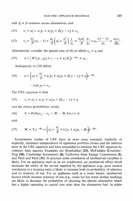
A second method of obtaining a discrete/continuous demand system is to start from a parametric specification of the UEC equation, treat Roy's identity as a partial differential equation whose solution defines a conditional indirect utility function, and then define the discrete choice probabilities from the indirect utility function. This procedure can be carried through for functions in which UEC levels exhibit some incorme elasticity.

First consider systems in which the UEC equation is linear in income,

(5) x = -Bj( y ri) + tmi(p1 l P2) + pli

with m/ linear in parameters and the distribution of v1i depending in general on discrete choice i. A general solution for an indirect utility function yielding this demand equation is

( 6) A ( '[(Pt l P 2) +.Y - ri + I'il/j]e P 2 P? 2i )

where

(7) M'(P I P2) = fm'(Q p2)e''@P''- dt

and 4 is a function which is increasing in its first argument.7 The demand for substitute energy satisfies

(8) x2= M2i(P ' P2) --e 2/1

where M' = M'1/)p, and 4)2/4'i = (a4/ap2)/(8;4/0p1) is evaluated at the argu- ments in (6).

Consider a special case of (6) in which '2i = P2 is the same for all i. The discrete choice probabilities satisfy

(9) P = ProbP [ Mi(P nP2)+. r + I81A//e A

> rbjM '(P I P2) +? V --- lj +

A special case of this system which yields simple functional form is

(10) u = In a ' + +cPi + ar+ I y-) + vlije43P} - aIn P2

6A function V( 1, P, P2) of normalized income and prices is the indirect utility function of some locally nonsatiated utility function if and only if it is lower semicontinuous, quasi-convex, increasing in i', nonincreasing in (pi, p2). and has V(tX,XpI,pP2) nondecreasing in X.

'Additional restrictions on 41 and Mi will be imposed by the lower semicontinuity, monotonicity. and quasi-convexity of the indirect utility function.


with f3i = /3 common across alternatives, and

(11l) x=-a' + a'p + p2+(y-ra)+,

(12) x2 = ~a5 - l)+ (ao+f$4 + - +a5a a___+ av (i2) 3 ( /? ) P2 / P2 P2 + ,2

Alternatively, consider the special case of (6) in which vli = q and

(13) U =[Mi(p, ' P2) +Y - ri + ii//3i]e -iP' + '2i

Analogously to (10) define

(14) a= (ap,+ , bPi + aTP2 + 83(y-ri) + 7)e

a5ln P2 + V2i

The UEC equation is then

(15) x =a aI+ ap, +i2P2 + 3(y- ri) + 7

and the choice probabilities satisfy

(16) Pi-Prob(v21- V2i< Wi Wj forlj # i)

with

(17) WY=VKe-&' =(a' + +a'p3)

Econometric studies of UEC have in most cases assumed, implicitly or explicitly, statistical independence of appliance portfolio choice and the additive error in the UEC equation and have proceeded to estimate the UEC equation by ordinary least squares. Examples are Houthakker [23], McFadden-Kirschner- Puig [30], Cambridge Systematics [6], California State Energy Commission [5], and Parti and Parti [31]. In practice some correlation of unobserved variables is likely. For an appliance such as an air conditioner, an unobserved effect which increases the utility of the service supplied by the appliance (e.g., poor natural ventilation in a housing unit) is likely to increase both its probability of selection and its intensity of use. For an appliance such as a water heater, unobserved factors which increase intensity of use (e.g., tastes for hot water clothes washing) are likely to decrease the probability of choosing the electric alternative which has a higher operating to capital cost ratio than the alternative fuel. In either


case, ordinary least squares estimation of the UEC equation induces a classical bias due to correlation of an explanatory variable and the equation error.8

In our empirical work, we adopt the specifications (15)-(17) with modifica- tions to accommodate varying climate and household characteristics and employ statistical procedures which are consistent in the presence of the suspect correlation.

3. A SPACE AND WATER HEAT CHOICE MODEL

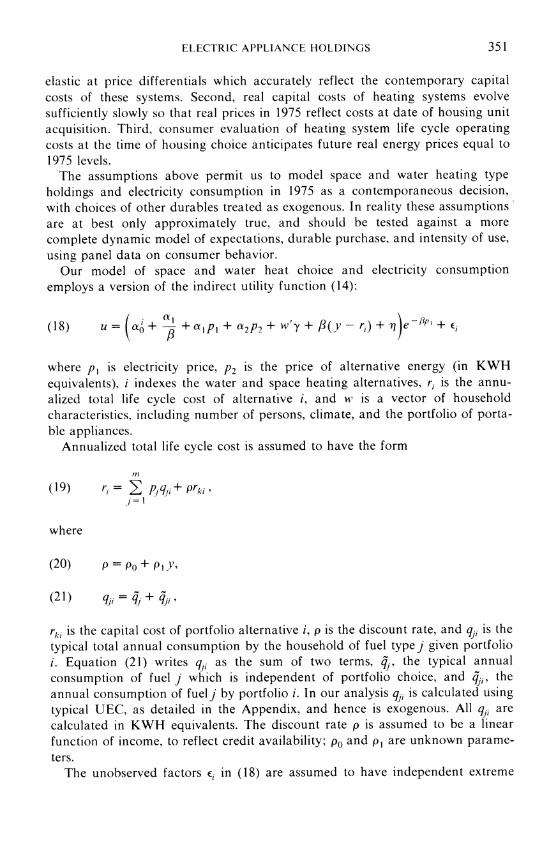
Household demand for electricity is determined by choice of space and water heating fuel type. ownership of electrical appliances such as an air conditioner, range, dishwasher, clothes dryer, and color T.V., and the intensity of use of these devices. Table I summarizes typical saturations and UEC's.

Our analysis isolates the space and water heating choice, treating the portfolio of other appliances owned by the household as statistically exogenous. The space and water heating choice is usually associated with selection of a housing unit. This choice is often made at a different point in time than purchase or retrofit decisions on portable appliances, so that a hypothesis of behavioral independence is plausible.

We make the following assumptions on housing market behavior: First, the supply of housing units of each heating fuel type is assumed to be perfectly

TABLE I

TypicAi. APPIJANCE SATURATIONS AND UEC

Appliance Saturation" O ECF'

Electric space heat .23 6440c Electric water heat .23 343Id Dishwasher .49 1453c Central air conditioner .39 2856f Room air conditioner .37 413 Freezer .56 1340 Electric range .67 780 Color TV .81 480 Electric dryer .56 1030

'From WCMS survey, 1975. subsample of 313 houscholds. bAnnual consumption in KWH, from BLS survey, 1972, fitted by regres-

sion of consumption on household appliance dunimies. (These estimates are suLbject to the potential bias discussed in the text.)

'the average number of heating degree days per year is 4318. dExcludes hot water consumption by a dishwasher. IUEC determined by hot water consumption if electiic water heat. fThe average number of cooling degree days per year is 1229. gAverage number of room air conditioners/number of householkis.

8Alternatively, an ordinary least squares regression of individually metered consumption by appliance for a sample of households who have chosen portfolios containinig this appliance induces a sample selection bias, with positive UEC residuals and low electricity prices more common in appliance holding households.


elastic at price differentials which accurately reflect the contemporary capital costs of these systems. Second, real capital costs of heating systems evolve sufficiently slowly so that real prices in 1975 reflect costs at date of housing unit acquisition. Third, consumer evaluation of heating system life cycle operating costs at the time of housing choice anticipates future real energy prices equal to 1975 levels.

The assumptions above permit us to model space and water heating type holdings and electricity consumption in 1975 as a contemporaneous decision, with choices of other durables treated as exogenous. In reality these assumptions' are at best only approximately true, and should be tested against a more complete dynamic model of expectations, durable purchase, and intensity of use, using panel data on consumer behavior.

Our model of space and water heat choice and electricity consumption employs a version of the indirect utility function (14):

(18) u = a, + a2P2 + w y + ,B(y-r) + q e -I@PI + (

where p, is electricity price, P2 is the price of alternative energy (in KWH equivalents), i indexes the water and space heating alternatives, ri is the annualized total life cycle cost of alternative i, and w is a vector of household characteristics, including number of persons, climate, and the portfolio of portable appliances.

Annualized total life cycle cost is assumed to have the form

InP

(19) r1= E q>i+ prai, 1=11

where

(20) p Po + Ply,

(21) qj= qj + Qii

rk, is the capital cost of portfolio alternative i, p is the discount rate, and qj1 is the typical total annual consumption by the household of fuel type j given portfolio i. Equation (21) writes qji as the sum of two terms, q7, the typical annual consumption of fuel j which is independent of portfolio choice, and qj,, the annual consumption of fuelj by portfolio i. In our analysis q11 is calculated using typical UEC, as detailed in the Appendix, and hence is exogenous. All q.. are calculated in KWH equivalents. The discount rate p is assumed to be a linear function of income, to reflect credit availability; Po and p, are unknown parameters.

The unobserved factors E in (18) are assumed to have independent extreme


value distributions,

(22) Prob(, < e = exp( - e - Y7/ X )

where -y =.577 ... is Euler's constant. The distribution of 'q conditional on (. ..E, ,]) iS assumed to have mean (X2 a/X)','_ R1i, and variance a2( -

Em_1 R,2) where 5E4t_U Ri = 0 and ,1 Rs,2 < I. Then Ri is the correlation of q and ,, ,E has unconditional mean zero and unconditional variance X2/2, and i1 has

unconditional mean zero and unconditional variance j`. The expected value of E, given that portfolioj is clhosen satisfies

|-In P A/ r'_1_ if i=j, (23) E[;I86(e)= I] _p

K -PIn Pi -Xr 3/7 if V/

where 8 (e) is an indicator random variable which is one if and only if j is the chosen alternative.

It then follows that

(24) E(-q 8j(()= l)= R[ P nP R l 1

The portfolio choice probabilities have a nonliriear multinomial logit form

(25) Pi = Prob[ u > 1i, forj v i]

= Prob [- < ( -- A/ 3(p(q, - q11) + p?(q2( - ))

-/3p(rk, - rk,))eP forjP f i

exp [( a' - 13(pq I + p2q21) -Iprk-)(e fe )/O]

exp [a( - A (P I q i.;q + p2q2J) -3prk/)(e HP )/]

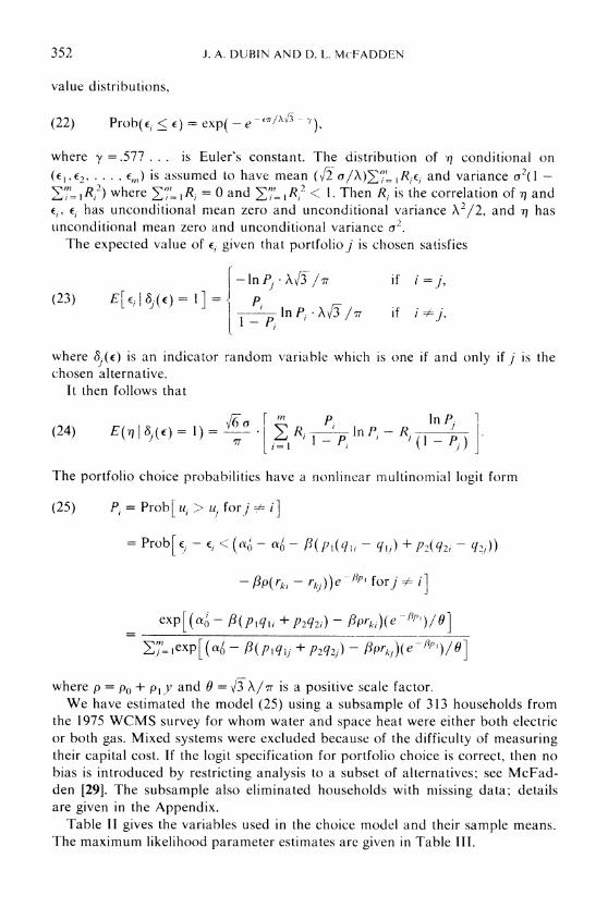
where p = po + pi y and 0 = H 3 X/ST is a positive scale factor. We have estimated the model (25) using a subsample of 313 households from

the 1975 WCMS survey for whom water and space heat were either both electric or both gas. Mixed systems were excluded because of the difficulty of measuring their capital cost. If the logit specification for portfolio choice is correct, then no bias is introduced by restricting analysis to a subset of alternatives; see McFad- den [29]. The subsample also eliminated households with missing data; details are given in the Appendix.

Table II gives the variables used in the choice model and their sample means. The maximum likelihood parameter estimates are given in Table III.


TABLE II

VARIABLES IN THE WATER-SPACE HEAT CHOICE MODEL

Means by Alternative

Electric Gas space and space and

Variable Mnemonic water water

Choice Dummy Choice .2332 .7668 Annual operating cost ($) piopa 392.8 208.0 Capital cost ($) PICPb 996.1 1136.0 Capital Cost- Income PICPY 17160. 20100.

($ 103$) Gas availability index GASA V751 .7294 0

in alternative one Marginal price of electricity WMPE751 .02194 0

in alternative one Electricity price ($/KWH) Pe p P, WMPE75 .02194 .02194 Gas price ($/KWH equivalent) Pg, P2, MPG75 .006449 .006449 Annual typical electric demand qli 17570. 6432.

(KWH) Annual typical gas demand q2i 0. 11138.0

(KWH equivalent) Income (103) y 14.97 17.55

b plCp rk,

TABLE III

ESTIMATED WATER-SPACE HEAT CHOICE MODEL

Alternative Frequency Proportion

Electric water and space 73 23.32 Gas water and space 240 76.68

313 100.00

Estimated Standard Asymptotic Explanatory Variable Coefficient Error t-Statistic

Capital Cost (PICP) - 0.0229 0.0084 - 2.73 Capital Cost * Income (103)

(PICP Y) 0.621 0.244 2.55 Annual Operating Cost

(PIOP) - 0.0604 0.026 - 2.29 Gas availability in

alternative one (GASA V751) -7.16 3.49 -2.05

Alternative one dummy (C1) -1.32 2.32 -0.57

Marginal price of electricity in alternative one (WMPE751) 496.77 228.20 2.18

Utility scale factor Exp((-,8)* WMPE75) - 39.09 14.30 - 2.73

Log Likelihood: at convergence - 102.4 with alternative

dummy only - 217.0


Note that the coefficients of PIOP, PICP, and PICPIY are -,8//, &Po/9H, and - /3p1/9, respectively. From the estimates of these parameters and their asymptotic covariances, one obtains the linear-in-income predicted discount factor

(26) A

= 0.3793 - 0.01028 (Annual Income)

(0.0780) (0.00289)

with annual income in thousands of 1975 dollars and standard errors in paren- theses. The negative estimate of p, implies that the discount rate declines with income. This result is consistent with a similar finding of Hausman [17]. The formula yields a predicted discount factor of 0.205 at the sample mean income of $16,948. Classical economic consumers who are not credit constrained can be expected to have discount factors equal to the real interest rate plus depreciation rate, roughly 0.10 to 0.15. This range is attained for households with incomes over $22,300. Households below this income level appear to be credit constrained. However, it should be noted that failure of consumers to correctly anticipate energy price increases between the time of housing choice and 1975, or an imperfectly elastic housing market in which the capital cost variable PICP overestimates the implicit capital cost component in the price of houses with systems which have higher expected operating costs in 1975 than at the time of construction, both introduce specification errors which bias upward the estimate of p.

Observe from Table III that we have defined a'= (yo GASA V75 + YIPe + 72) C l i . It then follows that the elasticity of demand for alternative i with respect to the price of electricity satisfies

(27) aInpe Pe o e3(Cl -P0 + 0) I Pjlnt eK9)

( 0 )( yI ee)e<jP

Noting that (y,1/) and (-,8//) are respectively the coefficients of WMPE751 and PIOP in Table III and that /3 is estimated in the utility scale factor term e-:P.! the elasticities calculated at the means of right-hand side variables are -0.473 for electric water and space heat and +0.144 for gas. For the price of gas, the elasticity is given by the analogue of (27) with 4ej replaced by gas consumption (in KWH equivalents); the elasticity of Pi with respect to the price of gas is

(28) e P -, ( ,

For the electric and gas portfolios these are + 1.41 and -0.43 respectively.


4. THE DEMAND FOR ELECTRICITY

Application of Roy's identity to (18), taking into account the dependence of life cycle cost r1 on the price of electricity in (19), but treating the discount rate p as exogenous to the household, yields annual electricity demand conditioned on space and water heating choice i,

(29) x = q1 a +? I (1pI + a 2P2 +WY +/3( r ) + rq.

A more convenient form for estimation is

m m (30) x- = q aj68 + a + a21 + wt'y + /3 , - E POP/ )

m

-3p0 jPICj djI+ 2

j=l =

where & is a dummy variable which is one when i =j. The postulated distribution of qj and E1 implies Eq = 0 and

(31) E(q i) =U]6 1 -Pj in I I-2 nPi

M l R1T j (R 1 ,I ) Pi j( i

mn GN 6Rj ] I p.

One can estimate (29) using ordinary least squares, and by three alternative methods which are consistent in the presence of correlation of the residual qj and the choice dummies :

(i) INSTRUMENTAL VARIABLE METHOD: The estimated probability, Pi, from the discrete choice model is used as an instrument for &: the list of instruments ispi,p2, w,y-ZJVPIOPj P I, 7PICPjP, and PI, ... P. n

(ii) REDUCED FORM METHOD: Ordinary least squares is applied to the equation

m m

(32) x - ai= E Pj+ alp, + a2P2 + w 'Y + - PIoP PI

m

-p PICPj Pj +i j(T

(iii) CONDITIONAL EXPECTATION CORRECTION METhIoD: Ordinary least squares


TABLE IV

VARIABLES ENTERING THE ELECTRICITY DEMAND EQUATION

Variable Mnemonic Mean

Income less energy cost (chosen alternative)($) NETINC 16710. Capital cost (chosen alternative)($) PICPI 1044. Gas availability index if alternative one chosen GASA V751 .1509 Marginal price of electricity if alternative

one chosen WMPE751 .004526 If alternative one chosen A 1 .2332 If homeowner OWN .9457 Gas availability index GASA V75 .7294 Number of persons in household PERSONS 3.78 Number of rooms ROOMS 6.265 Marginal price of electricity ($/KWH) WMPE75 0.02194 Marginal price of gas ($/KWH equivalent) MPG75a 0.00645 Annual electricity consumption (KWH)

Households choosing alternative 1 - 24240. Households choosing alternative 2 8645.

aConversion factor equals 4.6597 x 10-2 so that marginal price of gas in dollars per KWH equivalent is (4.6597 x 10-2) x (marginal price of gas in dollars per therm). Details are given in the Appendix.

is applied to the equation

m m

(33) x - qli= a8i+ lp+a 2P2 + W' y + y _ E PIOPj. S* j= j

-,BP>LPICP j8i + --'+IP J= j jl =AYj

I _ p. + +i +42

where the terms involving estimated probabilities permit a consistent estimate of E(-q I i).

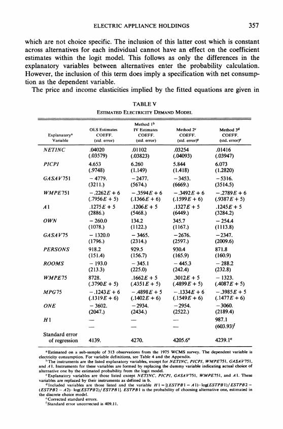
Table IV lists the variables included in the estimation of (30) and gives their sample means. Table V gives the ordinary least squares estimates of (30) as well as the estimates from the three procedures outlined above. These procedures utilized a corrected covariance matrix whose form was derived using the methods of Amemiya [2].9

Note that the dependent variable in (33) is net consumption defined above as the difference between annual electricity consumption and "typical electric usage" of appliances which are not included in the modeled portfolio decision. As a consequence, explanatory dummy variables indicating ownership of an electric clothes dryer, electric range, air conditioning system, color television, etc., are excluded from the demand specification.

Using net consumption as the dependent variable follows our definition of the annualized total cost ri. Recall that ri is defined as the operating plus discounted capital cost for alternative i plus the charge for typical fuel usage by appliances

9Dubin [9] presents the form of the corrected covariance matrix for each consistent procedure. Details are available on request.


which are not choice specific. The inclusion of this latter cost which is constant across alternatives for each individual cannot have an effect on the coefficient estimates within the logit model. This follows as only the differences in the explanatory variables between alternatives enter the probability calculation. However, the inclusion of this term does imply a specification with net consumption as the dependent variable.

The price and income elasticities implied by the fitted equations are given in

TABLE V

ESTIMATED ELECTRICITY DEMAND MODEL

Method lb

OLS Estimates TV Estimates Method 2c Method 3d

Explanatorya COEFF. COEFF. COEFF. COEFF. Variable (std. error) (std. error) (std. error)e (std. error)e

NETINC .04020 .01102 .03254 .01416 (.03579) (.03823) (.04093) (.03947)

PICPI 4.653 6.260 5.844 6.073 (.9748) (1.149) (1.418) (1.2820)

GASA V751 - 4779. -2477. - 3453. -5316. (3211.) (5674.) (6669.) (3514.5)

WMPE751 -.2262E + 6 -.3594E + 6 -.3492E + 6 -.2789E + 6 (.7956E + 5) (.1366E + 6) (.1599E + 6) (.9387E + 5)

A l .1275E + 5 .1206E + 5 .1327E + 5 .1245E-+ 5 (2886.) (5468.) (6449.) (3284.2)

OWN - 260.0 134.2 345.7 - 254.4 (1078.) (1122.) (1167.) (1113.8)

GA SA V75 - 1320.0 - 3465. -2676. -2347. (1796.) (2314.) (2597.) (2009.6)

PERSONS 918.2 929.5 930.4 871.8 (151.4) (156.7) (165.9) (160.9)

ROOMS - 193.0 - 345.1 - 445.3 - 288.2 (213.3) (225.0) (242.4) (232.8)

WMPE75 8728. .1662E + 5 .3012E + 5 - 1323. (.3790E + 5) (.4351 E + 5) (.4899E + 5) (.4087E + 5)

MPG75 -.1243E + 6 -.4898E + 5 -.1334E + 6 -.3985E + 5 (.1319E + 6) (.1402E + 6) (.1549E + 6) (.1477E + 6)

ONE - 3602. - 2934. -2954. -3060. (2047.) (2434.) (2522.) (2189.4)

HI - - 987.1 - ~~~~(603.93)1

Standard error of regression 4139. 4270. 4205.6e 4239.1e

a Estimated on a sub-sample of 313 observations from the 1975 WCMS survey. The dependent variable is electricity consumption. For variable definitions, see Table 4 and the Appendix.

bThe instruments are the listed explanatory variables, except for NETINC, PICPI, WMPE751 GASAV751, and A 1. Instruments for these variables are formed by replacing the dummy variable indicating actual choice of alternativc one by the estimated probability from the logit model.

cExplanatory variables are those listed except NETINC, PICPI, GASAV751, WMPE751, and Al. These variables are replaced by their instruments as defined in b.

d Included variables are those listed and the variable H I = [(ESTPB I - A I) - log(ESTPB l)/ESTPB2 -

(ESTPB2 - A2) log(ESTPB2)/ESTPB 1]. ESTPB I is the probability of choosing alternative one, estimated in the discrete choice model.

eCorrected standard errors. fStandard error uncorrected is 409.11.


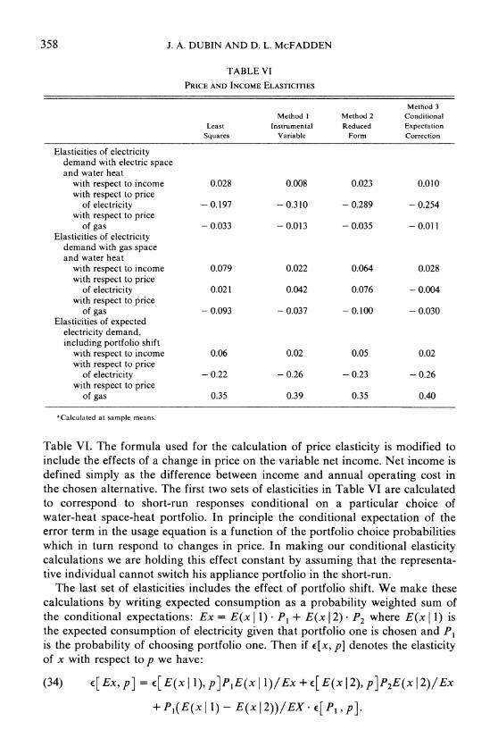
TABLE VI

PRICE AND INCOME ELASTICITIES

Method 3 Method I Method 2 Conditional

Least Instrumental Reduced Expectation Squares Variable Form Correction

Elasticities of electricity demand with electric space and water heat

with respect to income 0.028 0.008 0.023 0.010 with respect to price

of electricity - 0.197 - 0.310 - 0.289 -0.254 with respect to price

of gas - 0.033 - 0.013 - 0.035 -0.011 Elasticities of electricity

demand with gas space and water heat


of electricity 0.021 0.042 0.076 - 0.004 with respect to price

of gas -0.093 -0.037 -0.100 - 0.030 Elasticities of expected

electricity demand, including portfolio shift


of electricity - 0.22 -0.26 -0.23 - 0.26 with respect to price

of gas 0.35 0.39 0.35 0.40

aCalculated at sample means.

Table VI. The formula used for the calculation of price elasticity is modified to include the effects of a change in price on the variable net income. Net income is defined simply as the difference between income and annual operating cost in the chosen alternative. The first two sets of elasticities in Table VI are calculated to correspond to short-run responses conditional on a particular choice of water-heat space-heat portfolio. In principle the conditional expectation of the error term in the usage equation is a function of the portfolio choice probabilities which in turn respond to changes in price. In making our conditional elasticity calculations we are holding this effect constant by assuming that the representa- tive individual cannot switch his appliance portfolio in the short-run.

The last set of elasticities includes the effect of portfolio shift. We make these calculations by writing expected consumption as a probability weighted sum of the conditional expectations: Ex = E(x I 1) * P1 + E(x 1 2) P2 where E(x 1 1) is the expected consumption of electricity given that portfolio one is chosen and P1 is the probability of choosing portfolio one. Then if c[x, p] denotes the elasticity of x with respect to p we have:

(34) E[Ex, p] = c[E(xI 1), p]PIE(xI l)/Ex+e[E(x12),P]P2E(xI2)/Ex

+ PI(E(x I 1) - E(x I 2))/EX- * [P1 , p].


Each of the consistent procedures produced elasticities which are quantita- tively similar. Portfolio shifts are the primary contributor to the price sensitivity of average demand calculated from (34).

Comparing the final group of elasticities, we see that the elasticity of income is both smaller than the ordinary least squares estimates and considerably smaller than previous studies have shown. Own price elasticity is larger in magnitude for methods one and three than those given by ordinary least squares. Finally, we note that the cross-elasticity of the demand for electricity with respect to the price of gas (in KWH equivalents) is larger when estimated by consistent procedures one and three compared to the least squares estimates. Again the price sensitivity comes almost entirely from portfolio shift. Based on a qualitative comparison, reasonable point estimates for average demand under the consistent methods would be +0.02 for income elasticity, -0.26 for own price elasticity, and + 0.39 for cross-price-elasticity.

We have performed two tests of the independence of the choice variables and the error in (29). Method one, the instrumental variable method, was compared to the least squares estimates using the Wu-Hausman statistic.'0 The statistic T = ( - Es)'( VIV - VLS '(YIV - YLS) computed for the estimates in Table V on the suspected endogenous variables PICPI, GA SA V75 1, WMPE75 1, and A I is 15.07. (NETINC is excluded because to the limits of numerical accuracy it is perfectly correlated with its instrument.) Under the null hypothesis, this statistic is asymptotically Chi-squared with four degrees of freedom and thus exceeds the 95 per cent critical level of 9.49.

The second specification test compares the results of the least squares and Heckman methods of estimation and is identical to the Wald test of the significance of the "Heckman type" correction term."1 Recall that the variable H 1 entered as the conditional expectation correction factor in procedure three has coefficient (- aF6 R2/1r). This implies that the consistently estimated value of R2 is -0.299 with a standard error (corrected) of 0.179. The unadjusted standard error (given in Table V, footnote f) is correct for the null hypothesis of no correlation between q and . Under the null hypothesis of no correlation, the coefficient of H 1 would be zero. The asymptotic t statistic for the Wald test of this hypothesis is 2.41 which exceeds the 95 per cent critical level.'2

'0For details regarding this test see Hausman [15] and Hausman and Taylor [181. We wish to thank an anonymous referee for directing our attention to this identity derived in

Holly [22]. We should emphasize that the Heckman estimation method embodies specific assumptions regarding the joint distribution of q and e while the instrumental variable and reduced form methods are more robust in this sense. The appropriate degrees of freedom for Wu-Hausman tests using these latter estimation methods is four which is the number of dummies and their interactions whose exogeneity is under test.

The single degree of freedom in the Wu-Hausman test utilizing the Heckman estimation method reflects the imposition of the implicit distributional assumptions.

'2An alternative method of obtaining consistent estimates of the correlation coefficient R2 is to run an auxilary regression of the squared fitted residuals from procedures one, two, or three against an expression for conditional expectation given portfolio choice, evaluated at the estimated choice probabilities. The point estimates of R2 are -0.369, -0.337, and -0.332 respectively. These estimates are close to the estimate of - 0.299 obtained earlier from the coefficient of H1. Details of the calculation are available from the authors on request.


One might thus infer that an unobserved effect which increases the attractive- ness of all gas heat alternative tends to decrease simultaneously usage of electricity. This pattern could be produced, for example, by an unobserved marginal cost of electricity component.

We therefore reject the null hypothesis that the unobserved factors influencing portfolio choice are independent of the unobserved factors influencing intensity of use. If these results are confirmed in further analysis, one must conclude that estimation of UEC by least squares decomposition of total demand has the potential for severe bias, and that appropriate statistical methods, such as the instrumental variables procedure, are feasible and have satisfactory statistical properties.

Californiia Institute of Technology and

Massachusetts Institute of Technology

Manuscript received June, 1981; final revision received March, 1983.

APPENDIX

This section presents an account of variable construction and definition for the two-alternative all electric versus all gas water heat space heat choice model. The WCMS data survey with matched rate structure and temperature information consisted of 1502 observations. To have comparable information for both the water-heat space-heat model and the demand for electricity equation we selected a sample of 313 observations for which there were no missing observations and for which: (i) income, rate, and cost data were strictly positive (this included the marginal prices of electricity and gas in 1975 as well as space-heating capital costs as calculated by Hittman Associates for CSI/WEST); (ii) annual consumption of electricity in 1975 was positive; (iii) housing units used either gas or electric water-heat fuel and either gas or electric space-heat fuel but were selected so that the same fuel choice was made for both appliances in the portfolio; (iv) the date of housing construction was not before 1950.

WATER HEAT AND SPACE HEAT OPERATING COSTS

The definition of operating costs for water heaters and space heaters by fuel type is as follows:

Gas:

$/year = ($/therm-in)(therm-in/Btu-in)

(Btu-in/Btu-out)(Btu-out/KWH-out)

(KWH-out/KWH-in)(KWH-in/day)(days/year),

Electric:

$/year = ($/KWH-in)(KWH-in/day)(days/year),

where $/therm-in is marginal price of gas in 1975, $/KWH-in is marginal price of electricity in 1975, therm/Btu = 1/100000, Btu/KWH = 3413, Btu-in/Btu-out = 1/72, KWH-out/KWH-in =.983, KWH-in/day is average consumption. Average consumption for electric water heating depends on the number of residents. (See p. 5-13 of EPRI report EA-682, "Patterns of Energy Use by Electrical Appliances.")

Average consumption for electric space heat per day is related to the number of rooms in the


residence as well as the number of heating degree days. Heating degree days are the number of degrees the daily average temperature is below 65 degrees fahrenheit. Normally heating is not required when the outdoor temperature averages above 65 degrees. Using (BLS) data the following relationship was constructed:

KWH-in for electric 1] 9 - (.00217)(ANNUAL HDD) day space heat

+ (.000833)(ROOMS. ANNUAL HDD).

Note: Sample means and definitions for all variables may be found in Table II. The operating cost used in our econometric analysis differed in one minor respect. As discussed in

the text it proved useful to add the annual operating cost for base consumption of all other electric using appliances to the space heat operating cost. As this cost is constant across alternatives its inclusion allows one to think of the household as choosing a certain space heat-water heat portfolio as well as the portfolio of all other electric utilizing durables. This latter portfolio of durables is predetermined across the choices we are modelling.

Using the MRI survey we have constructed an electric utilization base rate which depends on the presence of appliance durables measured at their average or base usage rates. Thus, we have defined:

QEBASE = 2496 + (82.8 +.93 - CDD +.51 * ROOMS - CDD)

(Central Air Conditioning) + (- 144.6 + .447 * CDD)

- (Number of Room Air Conditioners) + 1340 . FOODFRZ

+ 780 - ELECRNGE + 480 CLRTV + 1030 * ECLTHDR

WATER HEAT AND SPACE HEAT CAPITAL COSTS

Capital costs for water heaters were not available within the WCMS data set. Estimates were obtained from the National Construction Estimator (Craftsman Book Co., Solano Beach, CA., 1978). These constructions again follow the specifications of CSI WEST (1979). They are then related to 1975 prices with a consumer price index adjustment.

Space heating capital costs for each fuel type were available within the WCMS matched data set. These numbers had been calculated using a residential thermal load model developed by Hittman Associates.

REFERENCES

[11 AMEMIYA, T.: "Regression Analysis when the Dependent Variable is Truncated Normal," Econometrica, 41(1973), 997-1016.

21 : "The Estimation of a Simultaneous Equation Generalized Probit Model," Econometrica, 46(1978), 1193-1206.

[3] AMEMIYA, T., AND G. SEN: "The Consistency of the Maximum Likelihood Estimator in a Disequilibrium Model," Tech. Report 238, Institute for Math. Studies in Social Sciences, Stanford, 1977.

[4] ANDERSON, K.: "Residential Energy Use: An Econometric Analysis," RAND Corporation, 1973.

[5] CALIFORNIA STATE ENERGY CONSERVATION: "California Energy Demand 1978-2000," Working Paper, 1979.

[6] CAMBRIDGE SYSTEMATICS/WEST: "An Analysis of Household Survey Data in Household Time- of-Day and Annual Electricity Consumption," Cambridge Systematics/West, Working Paper, 1979.

[71 DUBIN, J.: "Economic Theory and Estimation of the Demand for Consumer Durable Goods and Their Utilization: Appliance Choice and the Demand for Electricity," Massachusetts Institute of Technology Energy Laboratory Discussion Paper No. 23, MIT-EL 82-035WP, 1982.

[8] : "Rate Structure and Price Specification in the Demand for Electricity," mimeo, Massachusetts Institute of Technology, 1980.

[9] : "Two-Stage Single Equation Estimation Methods: An Efficiency Comparison," mimeo, Massachusetts Institute of Technology, 1981.


[10] DLJNCAN, G.: "Formulation and Statistical Analysis of the Mixed Continuous/Discrete Variable Model in Classical Production Theory," Econometrica, 48(1980), 839-852.

[11] FISHER., F., AND C. KAYSEN: A Study in Econometrics: The Demand for Electricity in the U.S. Amsterdam: North Holland, 1962.

[12] GOETT, A.: "A Structured Logit Model of Appliance Investment and Fuel Choice," Cambridge Systematics/West. Working Paper, 1979.

[13] GOLDFELD, S., AND R. QUANDT: "The Estimation of Structural Shifts by Switching Regressions," Annals of Economic and Social Measurement, 2(1973), 475-485.

[14] : "Techniques for Estimating Switching Regression" in Studies in Non-Linear Estimation, ed. by S. Goldfeld and R. Quandt. Cambridge: Ballinger, 1976.

[15] HAUSMAN, J.: "Specification Tests in Econometrics," Econometrica, 46(1978), 1251-1271. [16] -- : "Exact Consumer's Surplus and Deadweight Loss," American Economic Review,

71(1979), 663-676. [17] : "Individual Discount Rates and the Purchase and Utilization of Energy-Using

Durables," The Bell Journal of Economics, 10(1979), 33-54. [18] HAUSMAN, J., AND W. TAYLOR: "A Generalized Specification Test," Economic Letters, 8(1981),

239-245. [19] HAY, J.: "An Analysis of Occupational Choice and Income," Ph.D. Dissertation, Yale Univer-

sity, 1979. [20] HECKMAN, J.: "Dummy Endogenous Variables in a Simultaneous Equation System," Economet-

rica, 46(1978), 931-960. [21] : "Sample Selection Bias as a Specification Error," Econometrica, 47(1979), 153-162. [22] HOLLY, A.: "A Remark on Hausman's Specification Test," Econometrica, 50(1982), 749-759. [23] HOUTHAKKER, H.: "Some Calculations of Electricity Consumption in Great Britain," Journal of

the Royal Statistical Society, Series A, 114(1951), 351-371. [24] HOUTHAKKER, H., AND L. TAYLOR: Consumer Demand in the U.S., 2nd edition. Cambridge:

Harvard University Press, 1970. [25] LEE, L. F.: "Simultaneous Equations Models with Discrete and Continuous Variables," in

Structural Analysis of Discrete Data, ed. by C. Manski and D. McFadden. Cambridge: MIT Press, 1981.

[26] LEE, L. F., AND R. TROST: "Estimation of Some Limited Dependent Variable Models with Applications to Housing Demand," Journal of Econometrics, 8(1978), 357-382.

[27] MADDALA, G., AND F. NELSON: "Maximum Likelihood Methods for Markets in Disequilib- rium," Econometrica, 42(1974), 1013-1030.

[281 McFADDEN, D.: "Conditional Logit Analysis of Qualitative Choice Behavior," in Frontiers in Econometrics, ed. by P. Zarembka. New York: Academic Press, 1973.

[29] : "Econometric Models of Probabilistic Choice," in Structural Analysis of Discrete Data, ed. by C. Manski and D. McFadden. Cambridge: MIT Press, 1981.

[30] MCFADDEN, D., D. KIRSCHNER, AND C. PUIG: "Determinants of the Long-run Demand for Electricity," in Proceedings of the American Statistical Association, 1978.

[31] PARTI, M., AND C. PARTI: "The Total and Appliance-Specific Conditional Demand for Electric- ity in the Household Sector." Bell Journal of Economics, 11(1980), 309-321.

[32] TAYLOR, L.: "The Demand for Electricity: A Survey," Bell Journal of Economics, 6(1975), 74-110.

An Econometric Analysis of Residential Electric Appliance

Documents

Transcript of An Econometric Analysis of Residential Electric Appliance