An ecological stock-flow-fund modelling

framework

Yannis Dafermos, University of the West of England Giorgos Galanis, New Economics Foundation

Maria Nikolaidi, University of Greenwich

Abstract: This paper develops an ecological stock-flow-fund (ESFF) modelling framework that integrates the flow-fund model of Georgescu-Roegen (1971, 1979) with the stock-flow consistent modelling approach of Godley and Lavoie (2007). The ESFF framework combines various fundamental features of post-Keynesian and ecological economics, most notably the consideration of macroeconomy as an open subsystem of the closed ecosystem, the impact of aggregate demand on economic growth and employment, the biophysical limits to economic activity, the effects of finance on growth and the importance of the laws of thermodynamics. It is argued that the ESFF framework provides a quite rich platform for the analysis of the complex interactions between the macroeconomy and the ecosystem. Key words: Ecosystem, macroeconomy, laws of thermodynamics, ecological stock-flow-fund modelling. JEL codes: E1, E44, Q57

Preliminary and incomplete

Paper prepared for the 18th Conference of the Research Network Macroeconomics and Macroeconomic Policies (FMM), Berlin, 30 October-1 November 2014.

Address for correspondence: Yannis Dafermos, University of the West of England, Coldharbour Lane, Bristol, BS16 1QY, UK, e-mail: Yannis.Dafermos@uwe.ac.uk Acknowledgements: We are grateful to Sebastian Berger for constructive discussions and for drawing our attention to the work of Nicholas Georgescu-Roegen. We are also grateful to Andrew Mearman for valuable comments. An earlier version of this paper was presented at the 19th SCEME Seminar in Economic Methodology, Bristol, UK, May 2014. We wish to thank the participants for helpful comments. This research is part of the ‘Great Transition Project’ of the New Economics Foundation. The financial support from the Network for Social Change is gratefully acknowledged. The usual disclaimers apply.

1

1. Introduction

Over the last years the synthesis of ecological and post-Keynesian economics has been identified

as an important inquiry that can open the avenue for a fruitful combined examination of

economic and ecological issues (e.g. Holt and Spash, 2009; Mearman, 2009; Kronenberg, 2010;

Spash and Ryan, 2012; Fontana and Sawyer, 2013). Ecological economics provides a solid

framework for the analysis of the economy-ecosystem interactions. This framework is based on

the conceptualisation of the economy as an open subsystem of the closed ecosystem and the

detailed analysis of the implications of the First and the Second Law of Thermodynamics. Post-

Keynesian economics provides a quite rich explanation of the dynamics of modern capitalist

economics by putting at the centre of its analysis the importance of aggregate demand, the non-

neutral role of money and finance, the impact of fundamental uncertainty on economic

decisions and the links between income distribution and economic activity. Ecological

economics lacks the solid macroeconomic framework of post-Keynesian economics. Post-

Keynesian economics almost totally ignores the ecological constraints of macroeconomic

activity. Therefore, the synthesis of these two branches of economics would be a significant step

forward.

Although the importance of this synthesis has been recognised by a plethora of scholars, only a

few attempts have been made in developing an integrated approach in this direction and, even

more, in developing a modelling framework that combines ecological and post-Keynesian

economics in a systematic way. The most important of these attempts can be found in Victor and

Rosenbluth (2007), Victor (2012) and Barker et al. (2012) who have presented large-scale

models with Keynesian features that take into account the energy sector and various

environmental issues. Moreover, Jackson (2011), Fontana and Sawyer (2013) and Rezai et al.

(2013) have put forward building blocks for modelling frameworks that could combine

ecological economics with Keynesian (or post-Keynesian) insights. Although these contributions

are very significant, they can only be considered as the first steps towards the integration of

ecological with post-Keynesian economics. For example, in the aforementioned contributions

the role of money and finance, which is fundamental in post-Keynesian economics, is not

explicitly incorporated. Moreover, the full implications of the fact that the macroeconomy is an

open subsystem of the closed ecosystem are not analysed in an integrated way.

This paper develops a new modelling framework that synthesises post-Keynesian and ecological

approaches. This framework integrates the post-Keynesian stock-flow consistent (SFC)

2

modelling approach, developed by Godley and Lavoie (2007), with the flow-fund model of

Georgescu-Roegen (1971, ch. 9; 1979). The stock-flow consistent approach makes a coherent

analysis of the stocks and flows in the macroeconomy and the financial system allowing thereby

a consistent formulation of the links between the real and the financial spheres of the economy.

The flow-fund model of Georgescu-Roegen is an analytical framework that describes in detail

the energy and matter flow interactions of the economy with the environment as well as the role

of funds in the economic processes. The formulation of these interactions takes explicitly into

account the First and the Second Law of Thermodynamics. By combining and extending these

approaches, our ecological stock-flow-fund (ESFF) modelling framework incorporates

fundamental features of both post-Keynesian and ecological economics, most notably the

consideration of macroeconomy as an open subsystem of the closed ecosystem, the impact of

aggregate demand on economic growth and employment, the biophysical limits to economic

activity, the effects of finance on growth and the importance of the laws of thermodynamics.

The paper is organised as follows. Section 2 describes the main features of the ESFF modelling

framework. Section 3 presents the matrices and the equations of a simplified ESFF model.

Section 4 outlines some potential applications of our framework. Section 5 concludes.

2. Main features of the ESFF modelling framework

Over the last decade or so, stock-flow consistent (SFC) modelling has become a very popular

technique in post-Keynesian macroeconomics. Following the contributions of Godley (1999),

Lavoie and Godley (2001-2) and Godley and Lavoie (2007), various post-Keynesian

macroeconomists have used SFC models to analyse a plethora of macroeconomic issues.1 SFC

models rely on the use of balance sheet and transactions matrices which allow the explicit

consideration of the dynamic interactions between flows (e.g. interest, profits, wages) and stocks

(e.g. loans, deposits, equities). The integration of accounting into dynamic macro modelling

permits the detailed exploration of the links between the real and the financial spheres of the

macroeconomy and illuminates the non-neutral role of money and finance.

However, a prominent drawback of the SFC models is the absence of any analysis of the

transformation of matter and energy that takes place due to the economic processes. In SFC

models it is assumed that the energy and matter that are necessary for production and

1 See, for example, Le Heron and Mouakil (2008), Zezza (2008), van Treeck (2009), Dafermos (2012) and Nikolaidi (2014). See also Caverzasi and Godin (2014) for a recent review of the post-Keynesian stock-flow consistent modelling literature.

3

consumption are available without limit. Therefore, provided that there are no capital or labour

constraints, the output of the economy is demand-determined and, hence, if an adequate policy

mix is implemented, economic growth is theoretically feasible for an infinite period of time.

This feature comes in stark contrast with the fundamental propositions of ecological economists

that the macroeconomy is an open subsystem of the closed ecosystem2 and that economic

activity unavoidably respects the laws of thermodynamics.3 Ecological economists point out

that, in line with the First Law of Thermodynamics, the macroeconomy continuously uses

energy and matter inflows from the ecosystem and continuously produces waste which is an

outflow to the ecosystem. Moreover, it is argued that by converting low-entropy materials (e.g.

fossil fuels) into high-entropy materials (e.g. waste), macroeconomic activities tend to increase

the entropy in the ecosystem. This stems from the Second Law of Thermodynamics and suggests

that current economic activity reduces the ability of the macroeconomy to reproduce itself in the

future.

The flow-fund model of Georgescu-Roegen (1971, ch. 9; 1979) provides an adequate platform for

the consideration of these ecological limits. Using as a basis the First and the Second Law of

Thermodynamics, this model explicitly formulates the transformation of energy and matter that

takes places due to the economic processes. It also presents in detail the energy and matter links

between the various economic processes. Therefore, the biophysical limits to economic activity

are explicitly considered.

In the flow-fund model of Georgescu-Roegen the conceptualisation of production and

consumption relies on the distinction between the stock-flow resources and the fund-service

resources (see also Mayumi, 2001 and Daly and Farley, 2011). The stock-flow resources (such as

fossil fuels and minerals) are materially transformed into what they produce, can theoretically

be used at any rate desired and can be stockpiled for future use. The fund-service resources

(such as labour and capital) are not embodied in the output produced, can be used only at

specific rates and cannot be stockpiled for future use. The distinction between these two types of

resources is significant basically for two reasons. First, it points out that production needs both

fund-service and stock-flow resources, and there is no possibility to substitute the one with the

other. In conventional presentations of the production function this is not the case as capital,

2 In thermodynamics, an open system is a system that exchanges both energy and matter with its surrounding environment. A closed system exchanges only energy, not matter. An isolated system exchanges neither energy nor matter. 3 For a presentation of the laws of thermodynamics and their implications for economics see e.g. Amir (1994), Baumgärtner (2002) and Daly and Farley (2011).

4

labour and natural resources are described as ‘factors of production’ without a clarification of

their different role; it is also argued that perfect substitutability is possible. Second, the

distinction between stock-flow and fund-service resources is crucial for our understanding of

biophysical limits: it emphasises that while people cannot use the services of fund resources at

the rate that they wish, they can do so with the stock-flow resources. This implies that the stock-

flow resources can be exhausted in a short period of time if people decide to increase

substantially the associated flow rate.

The ESFF framework put forward in this paper is a synthesis of the post-Keynesian SFC models

and the flow-fund model of Georgescu-Roegen. This synthesis allows us to combine the

aforementioned advantages of these two approaches. The ESFF modelling framework relies on

four matrices: 1) the energy-matter flow-fund matrix; 2) the energy-matter stock matrix; 3) the

transactions flow matrix; 4) the balance sheet matrix. The first matrix is an extension of

Georgescu-Roegen’s (1979, p. 1042) flow-fund matrix and captures the energy and matter flows

in the ecosystem as well as the funds are necessary for the various economic and natural

processes. The second matrix represents the stock of matter and energy in the ecosystem. The

third and the fourth matrix describe the changes in the stocks and flows of the macroeconomic

and financial systems, following the traditional formulations in SFC literature.

3. Matrices and equations

The ESFF modelling framework will be presented by postulating a highly simplified

macroeconomy and a highly simplified ecosystem. In particular, we consider a closed

macroeconomy in which there is no government and no central bank. Firms make conventional

and green investment by using their retained profits and by taking out loans from commercial

banks. Households do not take on debt. Commercial banks distribute all their profits to

households. There is one type of good in the economy that can be used for both consumption

and investment purposes. Firms produce this good by employing controlled energy and

controlled matter from the ecosystem. Controlled energy is produced by using energy in situ.

Controlled matter is produced by using matter in situ. Firms recycle a part of their waste which

is then used as an inflow in the production of the investment and consumption goods.

Depreciation of capital is assumed away. There are no durable goods and no houses. Households

consume all the goods within one period. The price level is set equal to unity; this implies that

real and nominal variables coincide.

5

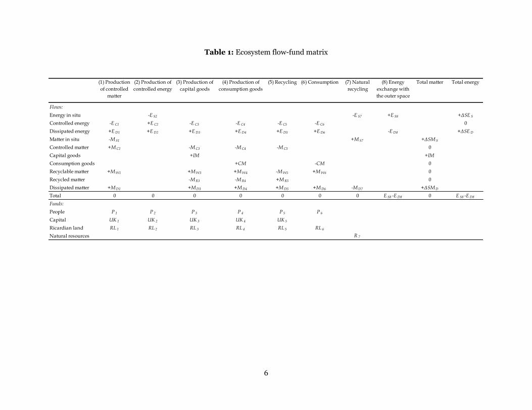
Table 1 depicts the ecosystem flow-fund matrix. The matrix illustrates the changes in the matter

and energy of the ecosystem as a result of economic and natural processes. It also shows the

funds that are necessary for each process. The upper part of the matrix indicates flows of energy

and matter. These flows are expressed in kilograms (they could also be expressed in kilojoules).

Symbols with a plus sign illustrate inflows to the ecosystem. Symbols with a minus sign indicate

outflows from the ecosystem. The lower part of the matrix captures funds.

The matrix presents the following economic and natural processes:

(1) Production of controlled matter: It produces controlled matter using matter in situ and

controlled energy.

(2) Production of controlled energy: It produces controlled energy using energy in situ.

(3) Production of capital goods: It produces capital goods using controlled energy, controlled

matter and recycled matter.

(4) Production of consumption goods: It produces consumption goods using controlled energy,

controlled matter and recycled matter.

(5) Recycling: It produces recycled matter using recyclable matter, controlled energy and

controlled matter. This recycling is conducted by firms.

(6) Consumption by households.

(7) Natural recycling: It produces matter in situ using dissipated matter and controlled energy.

This recycling stems from nature’s waste absorption capacity.

(8) Energy exchange with the outer space: It captures the fact that the ecosystem exchanges

energy with the outer space.

The first 7 columns in the upper part of the flow-fund matrix sum to zero. This is due to the First

Law of Thermodynamics which suggests that energy and mass are conserved in these processes.

The last two columns in Table 1 show the changes in the total matter and total energy of the

ecosystem. Since the ecosystem is a closed thermodynamic system, the total matter does not

change (and, hence, the respective column sums to zero) but the total energy does change (and,

therefore, the respective column does not sum to zero). Importantly, the flow-fund matrix is

also in line with the Second Law of Thermodynamics: dissipated energy and matter are

produced in the economic process leading to an increase in the entropy of the ecosystem.

6

Table 1: Ecosystem flow-fund matrix

(1) Production

of controlled

matter

(2) Production of

controlled energy

(3) Production of

capital goods

(4) Production of

consumption goods

(5) Recycling (6) Consumption (7) Natural

recycling

(8) Energy

exchange with

the outer space

Total matter Total energy

Flows:

Energy in situ -E S2 -E S7 +E S8 +ΔSE S

Controlled energy -E C1 +E C2 -E C3 -E C4 -E C5 -E C6 0

Dissipated energy +ED1 +ED2 +ED3 +ED4 +ED5 +ED6 -ED8 +ΔSED

Matter in situ -M S1 +M S7 +ΔSM S

Controlled matter +MC1 -MC3 -MC4 -MC5 0

Capital goods +IM +IM

Consumption goods +CM -CM 0

Recyclable matter +MW1 +MW3 +MW4 -MW5 +MW6 0

Recycled matter -MR3 -MR4 +MR5 0

Dissipated matter +MD1 +MD3 +MD4 +MD5 +MD6 -MD7 +ΔSMD

Total 0 0 0 0 0 0 0 E S8 -ED8 0 E S8 -ED8

Funds:

People P 1 P 2 P 3 P 4 P 5 P 6

Capital UK 1 UK 2 UK 3 UK 4 UK 5

Ricardian land RL 1 RL 2 RL 3 RL 4 RL 5 RL 6

Natural resources R 7

7

The lower part of the matrix indicates that people, capital and Ricardian land (i.e. land as a

location and physical substrate) are the necessary funds for the first five processes. In our

simplified framework, capital is not used as a fund in the consumption process. Natural

resources are the only fund in natural recycling.

Table 2 depicts the ecosystem stock matrix. This matrix shows the stock of matter and stock of

energy in the ecosystem, expressed in kilograms (these stocks could also be expressed in

kilojoules). The stock of matter and energy changes due to the inflows and outflows represented

in Table 1. Since the ecosystem is a closed thermodynamic system, the stock of total matter

remains unchanged, while the respective stock of total energy varies.

Table 2: Ecosystem stock matrix

Matter Energy

Matter in situ SM S

Capital stock KM

Dissipated matter SMD

Energy in situ SE S

Dissipated energy SED

Total SM SE

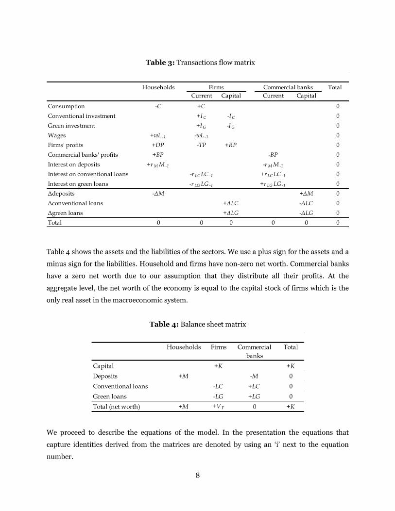
Table 3 and 4 represent the macroeconomic system. Table 3 is the transactions flow matrix. This

matrix shows the transactions that take place between the various sectors of the economy. For

each sector inflows are denoted by a plus sign and outflows are denoted by a minus sign. At the

aggregate level, monetary inflows should be equal to monetary outflows.

8

Table 3: Transactions flow matrix

Households Total

Current Capital Current Capital

Consumption -C +C 0

Conventional investment +IC -IC 0

Green investment +IG -IG 0

Wages +wL -1 -wL -1 0

Firms' profits +DP -TP +RP 0

Commercial banks' profits +BP -BP 0

Interest on deposits +r M M -1 -r M M -1 0

Interest on conventional loans -r LC LC -1 +r LC LC -1 0

Interest on green loans -r LG LG -1 +r LG LG -1 0

Δdeposits -ΔM +ΔM 0

Δconventional loans +ΔLC -ΔLC 0

Δgreen loans +ΔLG -ΔLG 0

Total 0 0 0 0 0 0

Firms Commercial banks

Table 4 shows the assets and the liabilities of the sectors. We use a plus sign for the assets and a

minus sign for the liabilities. Household and firms have non-zero net worth. Commercial banks

have a zero net worth due to our assumption that they distribute all their profits. At the

aggregate level, the net worth of the economy is equal to the capital stock of firms which is the

only real asset in the macroeconomic system.

Table 4: Balance sheet matrix

Households Firms Commercial

banks

Total

Capital +K +K

Deposits +M -M 0

Conventional loans -LC +LC 0

Green loans -LG +LG 0

Total (net worth) +M +V F 0 +K

We proceed to describe the equations of the model. In the presentation the equations that

capture identities derived from the matrices are denoted by using an ‘i’ next to the equation

number.

9

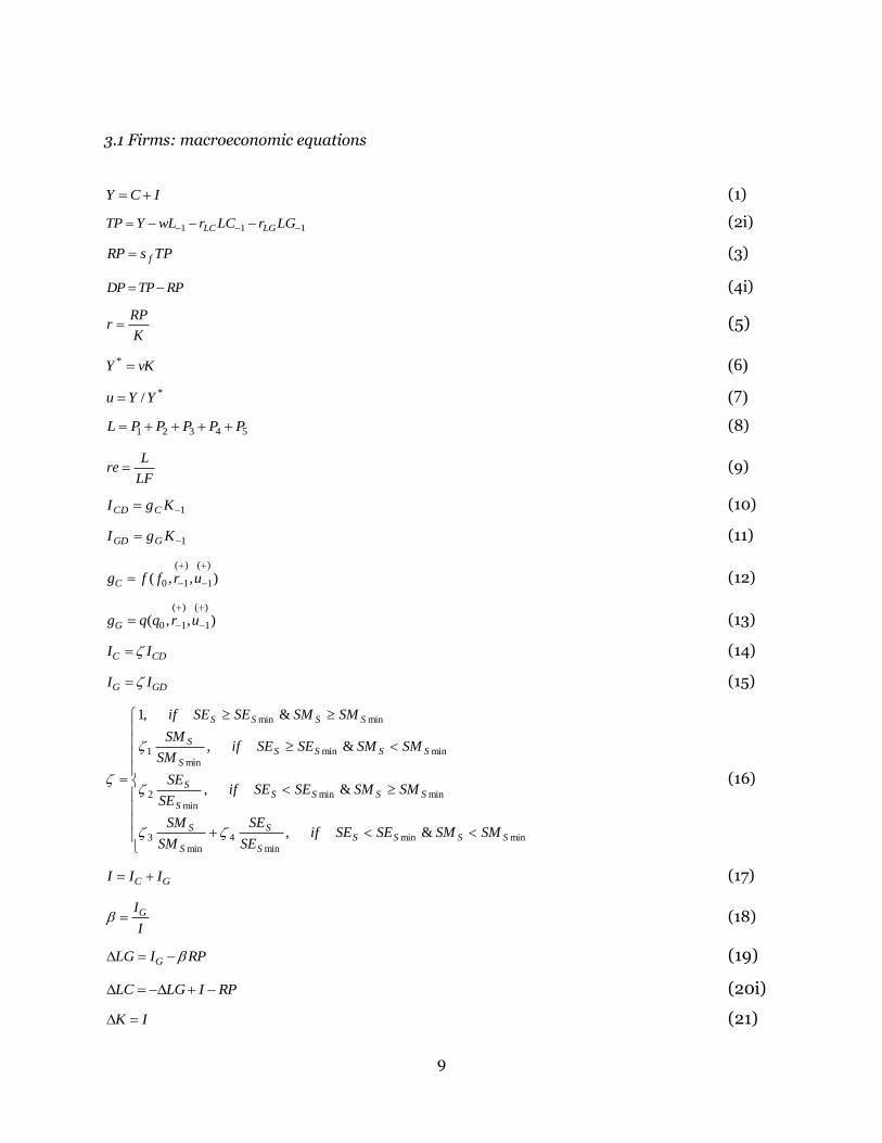
3.1 Firms: macroeconomic equations

Y C I (1)

1 1 1LC LGTP Y wL r LC r LG (2i)

TPsRP f (3)

DP TP RP (4i)

RPr

K (5)

vKY * (6)

*/ YYu (7)

1 2 3 4 5L P P P P P (8)

Lre

LF (9)

1 KgI CCD (10)

1 KgI GGD (11)

( ) ( )

0 1 1( , , )Cg f f r u

(12)

( ) ( )

0 1 1( , , )Gg q q r u

(13)

C CDI I (14)

G GDI I (15)

minminmin

4min

3

minminmin

2

minminmin

1

minmin

&,

&,

&,

&,1

SSSSS

S

S

S

SSSSS

S

SSSSS

S

SSSS

SMSMSESEifSE

SE

SM

SM

SMSMSESEifSE

SE

SMSMSESEifSM

SM

SMSMSESEif

(16)

C GI I I (17)

GI

I (18)

GLG I RP (19)

LC LG I RP (20i)

K I (21)

10

Equation (1) shows that the output of the economy ( Y ) is equal to the number of consumption

goods ( C ) plus the number of investment goods ( I ). The total profits of firms (TP ) are given by

equation (2i); w is the wage rate, L is the number of employed workers, LCr is the interest rate

on conventional loans, LGr is the interest rate on green loans, LC is the amount of conventional

loans and LG is the amount of green loans. Firms’ retained profits ( RP ) are a proportion ( fs ) of

their total profits (equation 3). The distributed profits of firms ( DP ) are determined as a

residual (equation 4i). Equation (5) gives the rate of retained profits ( r ); K is the total capital

stock of firms. The full-capacity output ( *Y ) is a function of the capital stock (equation 6); v is

the full-capacity output-to-capital ratio. The rate of capacity utilisation ( u ) is given in equation

(7). The total number of employed workers is equal to the sum of the people ( 54321 PPPPP )

that are used as a fund in the economic processes conducted by firms (equation 8). The rate of

employment ( re ) is given by equation (9); LF is the labour force.

Firms make two types of investment: (a) conventional investment ( CDI ) that does not affect

energy and matter efficiency (this efficiency is defined below); (b) green investment ( GDI ) that

increases energy and matter efficiency. In line with the conventional post-Keynesian

formulations of investment function, both investment rates rely on the rate of profit and the rate

of capacity utilisation (see equations 12 and 13). However, while the conventional investment

rate ( Cg ) is basically associated with the ‘animal spirits’ of entrepreneurs, reflected in 0f , the

green investment rate ( Gg ) is associated with some other factors, reflected in 0q . These factors

might pertain to environmental policy, the interest rate on green loans, the scarcity of matter

and energy in situ and the prices of natural resources.

Equations (14)-(16) show that the demand for investment goods, which is shown in equations

(10) and (11), is satisfied only when the stock of matter in situ ( SSM ) and the stock of energy in

situ ( SSE ) are above (or equal to) some certain thresholds ( minSSM and minSSE ). When

minSS SMSM and/or minSS SESE , only a proportion of the demanded investment goods is

produced ( 4,3,2,1,1 ii ). This happens because the available energy and matter in the

11

ecosystem is not enough to support the production of the investment goods and, thus, firms

cannot (or avoid to) satisfy all the demand.4

Equation (17) gives total investment. Equation (18) defines the ratio ( ) of green investment to

total investment. For simplicity, it is assumed that this ratio determines the proportion of

retained profits used for financing green investment. The rest finance is provided through green

loans that firms take out from banks (see equation 19). Equation (20i) shows the change in

conventional loans.5 The change in capital stock is given in equation (21).

3.2 Production of controlled matter

5431 CCCC MMMM (22i)

1111 CS MM (23)

1121 CC ME (24)

1131 CW MM (25)

1141 CD MM (26)

111111 DWCSCD MMMMEE (27i)

221111

11

1

SC

C

ME

Me (28)

)()(

11

GIwe (29)

)()(

114

GIy (30)

Equation (22i) shows that the controlled matter that firms need to produce ( 1CM ) is equal to the

controlled matter that is essential for the production of capital goods, consumption goods and

recycled matter ( 3CM , 4CM and 5CM , respectively). Equations (23)-(26) express the technology

that is used in the production of controlled matter; )4,3,2,1(,01 ii are technical coefficients.6

1SM is the matter in situ and 1CE is the controlled energy, both of which should be used as

inflows in order to produce 1CM . 1WM and 1DM are the recyclable waste matter and the

4 Equations (14)-(16) is a formulation of the general idea that economic growth can be restricted in the long run by

the biophysical limits. 5 By combining equations (17), (19) and (20i), we get: (1 )CLC I RP . 6 Equations (23)-(26) show relationships between masses but they implicitly reflect relationships between moles.

See Baumgärtner (2002) for some examples.

12

dissipated matter which are by-products of the process. The dissipated energy ( 1DE ), which is an

additional by-product of the process, is determined as a residual so as to ensure that the First

Law of Thermodynamics is satisfied (equation 27i).

The matter and energy efficiency of the process ( 1e ) is captured by equation (28). This

efficiency is defined as the ratio of controlled matter to the inflow of energy and matter (see

Ayres and van den Bergh, 2005 for similar definitions). Equation (27i) implies 11 e . It is

postulated that the change in efficiency relies positively on green investment (equation 29).

Moreover, green investment reduces the dissipated matter produced per kilogram of controlled

matter (equation 30).

3.3 Production of controlled energy

654312 CCCCCC EEEEEE (31i)

2212 CS EE (32)

222 CSD EEE (33i)

212

22

1

S

C

E

Ee (34)

)()(

22

GIwe (35)

Equation (31i) gives the controlled energy ( 2CE ) that is necessary to be produced by firms. This

is determined by the inflow of controlled energy which is essential for the other five economic

processes. Equation (32) shows that the energy in situ ( 2SE ) is determined according to the

technical coefficient 021 . Dissipated energy ( 2DE ) is determined as a residual (see equation

33i). The energy efficiency in the production of controlled energy ( 12 e ) is defined in equation

(34). Equation (35) illustrates that green investment improves energy efficiency.

3.4 Production of capital goods

IIM (36)

53 RR MM (37)

IMEC 313 (38)

13

3323 RC MIMM (39)

IMMW 333 (40)

IMM D 343 (41)

333333 DRWCCD MMMIMMEE (42i)

32313333

1

RCC MME

IMe (43)

)()(

33

GIwe (44)

)()(

334

GIy (45)

Equation (36) shows the mass of investment goods in kilograms ( IM ); denotes the kilograms

per good. Equation (37) illustrates that a proportion ( ) of the total recycled matter ( 5RM ) is

used as an inflow ( 3RM ) in the production of capital goods. Equations (38)-(41) capture the

technology that is used in the production of investment goods; )4,3,2,1(,03 ii are technical

coefficients. 3CE and 3CM are the controlled energy and the controlled matter that should be

used as inflows in order to produce IM . 3WM and 3DM are the recyclable waste matter and the

dissipated matter which are by-products of the process. The dissipated energy ( 3DE ), which is

an additional by-product of the process, is determined as a residual (equation 42i). Equation

(43) defines the energy and matter efficiency in the production of capital goods ( 13 e ). The

change in this efficiency is a positive function of green investment (equation 44). Moreover,

green investment reduces the dissipated matter produced per kilogram of investment good

(equation 45).

3.5 Production of consumption goods

CCM (46)

354 RRR MMM (47i)

CMEC 414 (48)

4424 RC MCMM (49)

CMMW 434 (50)

CMM D 444 (51)

444444 DRWCCD MMMCMMEE (52i)

14

42414444

1

RCC MME

CMe (53)

)()(

44

GIwe (54)

)()(

444

GIy (55)

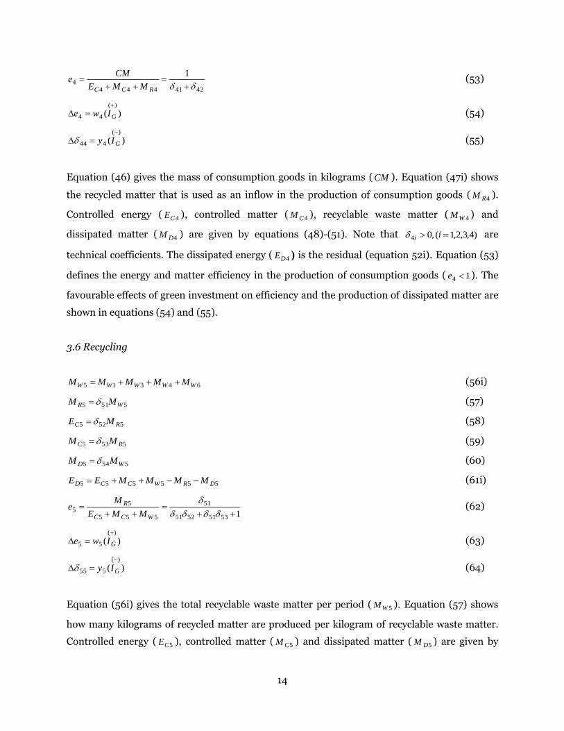
Equation (46) gives the mass of consumption goods in kilograms ( CM ). Equation (47i) shows

the recycled matter that is used as an inflow in the production of consumption goods ( 4RM ).

Controlled energy ( 4CE ), controlled matter ( 4CM ), recyclable waste matter ( 4WM ) and

dissipated matter ( 4DM ) are given by equations (48)-(51). Note that )4,3,2,1(,04 ii are

technical coefficients. The dissipated energy ( 4DE ) is the residual (equation 52i). Equation (53)

defines the energy and matter efficiency in the production of consumption goods ( 14 e ). The

favourable effects of green investment on efficiency and the production of dissipated matter are

shown in equations (54) and (55).

3.6 Recycling

64315 WWWWW MMMMM (56i)

5515 WR MM (57)

5525 RC ME (58)

5535 RC MM (59)

5545 WD MM (60)

555555 DRWCCD MMMMEE (61i)

153515251

51

555

55

WCC

R

MME

Me (62)

)()(

55

GIwe (63)

)()(

555

GIy (64)

Equation (56i) gives the total recyclable waste matter per period ( 5WM ). Equation (57) shows

how many kilograms of recycled matter are produced per kilogram of recyclable waste matter.

Controlled energy ( 5CE ), controlled matter ( 5CM ) and dissipated matter ( 5DM ) are given by

15

equations (58)-(60). Note that )4,3,2,1(,05 ii are technical coefficients. Identity (61i) shows

the dissipated energy ( 5DE ). The energy and matter efficiency ( 15 e ) is captured by equation

(62). Equations (63) and (64) show that 5e and 55 are affected by green investment.

3.7 People and capital fund-services in the production processes

iiii ple (65)

i

ii

QP

(66)

iiii khe (67)

i

ii

QUK

(68)

For equations (65)-(68) we have that 5,4,3,2,1i . Moreover: 11 CMQ , 22 CEQ , IMQ 3 ,

CMQ 4 and 55 RMQ . Labour productivity ( i ) is given by equation (65); il denotes the

energy and matter inflows used per person hour and ip denotes the hours per person employed.

Note that ii le is the useful output per person hour. This expresses the service rate of people (as a

fund in the production process). The number of people ( iP ) who work in each production

process is determined according to equation (66).

Capital productivity ( i ) is given by equation (67); ih denotes the energy and matter inflows

used per capital hour and ik denotes the hours per utilised capital. Note that ii he is the useful

output per capital hour. This expresses the service rate of capital (as a fund in the production

process). The utilised capital ( iUK ) in each production process is determined according to

equation (68).

3.7 Households: macroeconomic equations

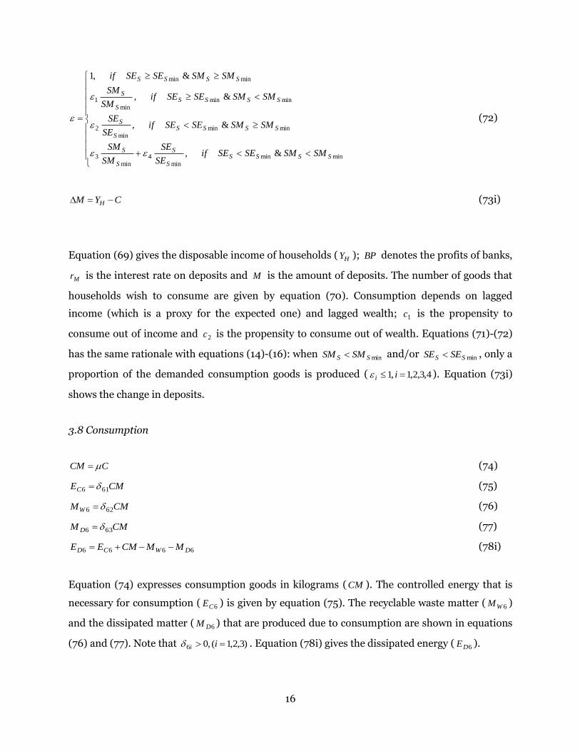
1 1H MY wL DP BP r M (69)

1 1 2 1D HC c Y c M (70)

DC C (71)

16

minminmin

4min

3

minminmin

2

minminmin

1

minmin

&,

&,

&,

&,1

SSSSS

S

S

S

SSSSS

S

SSSSS

S

SSSS

SMSMSESEifSE

SE

SM

SM

SMSMSESEifSE

SE

SMSMSESEifSM

SM

SMSMSESEif

(72)

HM Y C (73i)

Equation (69) gives the disposable income of households ( HY ); BP denotes the profits of banks,

Mr is the interest rate on deposits and M is the amount of deposits. The number of goods that

households wish to consume are given by equation (70). Consumption depends on lagged

income (which is a proxy for the expected one) and lagged wealth; 1c is the propensity to

consume out of income and 2c is the propensity to consume out of wealth. Equations (71)-(72)

has the same rationale with equations (14)-(16): when minSS SMSM and/or minSS SESE , only a

proportion of the demanded consumption goods is produced ( 4,3,2,1,1 ii ). Equation (73i)

shows the change in deposits.

3.8 Consumption

CM C (74)

CMEC 616 (75)

CMMW 626 (76)

CMM D 636 (77)

6666 DWCD MMCMEE (78i)

Equation (74) expresses consumption goods in kilograms ( CM ). The controlled energy that is

necessary for consumption ( 6CE ) is given by equation (75). The recyclable waste matter ( 6WM )

and the dissipated matter ( 6DM ) that are produced due to consumption are shown in equations

(76) and (77). Note that )3,2,1(,06 ii . Equation (78i) gives the dissipated energy ( 6DE ).

17

3.10 Banks: macroeconomic equations

1 1 1LC LG MBP r LC r LG r M (79i)

1LC Mr spr r (80)

2LG Mr spr r (81)

LGLCM (82-redmac)

The profits of banks are equal to the interest on both conventional and green loans minus the

interest on deposits (equation 79i). The interest rate on loans is equal to the interest rate on

deposits plus a spread (see equations 80 and 81); 1spr and 2spr denote the spreads for

conventional and green loans, respectively. Equation (82-redmac) is the redundant equation of

the macroeconomic system described in Table 3: it is logically implied by all the other equations

of this system.

3.11 Natural processes

DD SMM 7 (83)

SM

SM D10 (84)

7717 DS ME (85)

777 SDS EMM (86i)

8SE (87)

DD SEE 8 (88)

Equation (83)-(86i) capture the recycling that stems from nature’s waste absorption capacity.

Equation (83) shows that in each period the natural resources have the capacity to absorb (and

transform into matter in situ) only a (small) proportion ( 10 ) of the stock of dissipated

matter; 7DM is the dissipated matter that is recycled by nature. According to equation (84), the

capacity of the nature to recycle dissipated matter reduces as the stock of dissipated matter

increases relative to the total stock of matter. The energy in situ that is necessary for recycling

( 7SE ) is given by equation (85). Equation (86i) shows the matter in situ that is created from

natural recycling ( 7SM ).

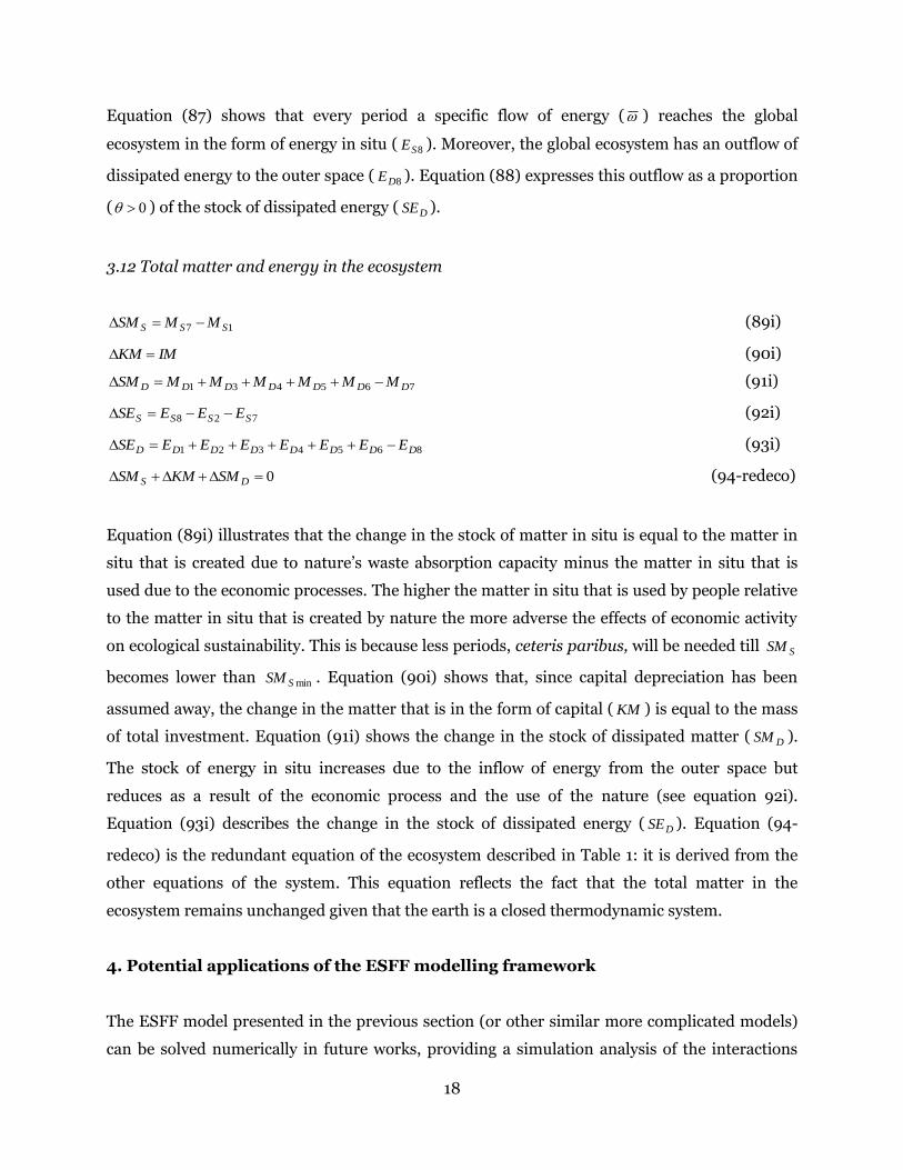
18

Equation (87) shows that every period a specific flow of energy ( ) reaches the global

ecosystem in the form of energy in situ ( 8SE ). Moreover, the global ecosystem has an outflow of

dissipated energy to the outer space ( 8DE ). Equation (88) expresses this outflow as a proportion

( 0 ) of the stock of dissipated energy ( DSE ).

3.12 Total matter and energy in the ecosystem

17 SSS MMSM (89i)

IMKM (90i)

765431 DDDDDDD MMMMMMSM (91i)

728 SSSS EEESE (92i)

8654321 DDDDDDDD EEEEEEESE (93i)

0 DS SMKMSM (94-redeco)

Equation (89i) illustrates that the change in the stock of matter in situ is equal to the matter in

situ that is created due to nature’s waste absorption capacity minus the matter in situ that is

used due to the economic processes. The higher the matter in situ that is used by people relative

to the matter in situ that is created by nature the more adverse the effects of economic activity

on ecological sustainability. This is because less periods, ceteris paribus, will be needed till SSM

becomes lower than minSSM . Equation (90i) shows that, since capital depreciation has been

assumed away, the change in the matter that is in the form of capital ( KM ) is equal to the mass

of total investment. Equation (91i) shows the change in the stock of dissipated matter ( DSM ).

The stock of energy in situ increases due to the inflow of energy from the outer space but

reduces as a result of the economic process and the use of the nature (see equation 92i).

Equation (93i) describes the change in the stock of dissipated energy ( DSE ). Equation (94-

redeco) is the redundant equation of the ecosystem described in Table 1: it is derived from the

other equations of the system. This equation reflects the fact that the total matter in the

ecosystem remains unchanged given that the earth is a closed thermodynamic system.

4. Potential applications of the ESFF modelling framework

The ESFF model presented in the previous section (or other similar more complicated models)

can be solved numerically in future works, providing a simulation analysis of the interactions

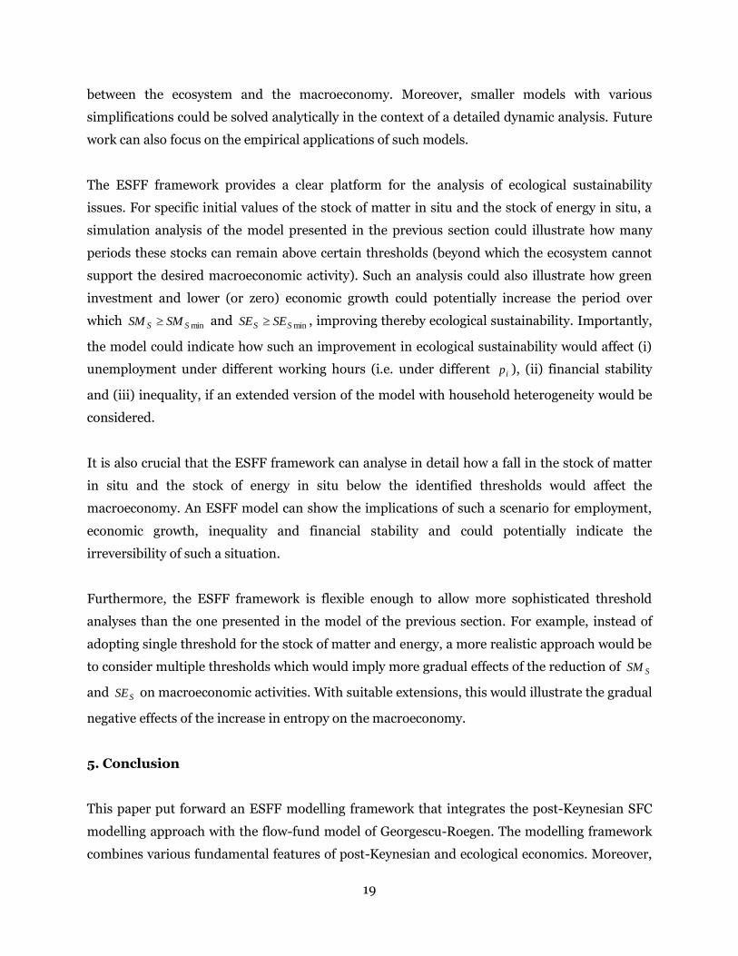
19

between the ecosystem and the macroeconomy. Moreover, smaller models with various

simplifications could be solved analytically in the context of a detailed dynamic analysis. Future

work can also focus on the empirical applications of such models.

The ESFF framework provides a clear platform for the analysis of ecological sustainability

issues. For specific initial values of the stock of matter in situ and the stock of energy in situ, a

simulation analysis of the model presented in the previous section could illustrate how many

periods these stocks can remain above certain thresholds (beyond which the ecosystem cannot

support the desired macroeconomic activity). Such an analysis could also illustrate how green

investment and lower (or zero) economic growth could potentially increase the period over

which minSS SMSM and minSS SESE , improving thereby ecological sustainability. Importantly,

the model could indicate how such an improvement in ecological sustainability would affect (i)

unemployment under different working hours (i.e. under different ip ), (ii) financial stability

and (iii) inequality, if an extended version of the model with household heterogeneity would be

considered.

It is also crucial that the ESFF framework can analyse in detail how a fall in the stock of matter

in situ and the stock of energy in situ below the identified thresholds would affect the

macroeconomy. An ESFF model can show the implications of such a scenario for employment,

economic growth, inequality and financial stability and could potentially indicate the

irreversibility of such a situation.

Furthermore, the ESFF framework is flexible enough to allow more sophisticated threshold

analyses than the one presented in the model of the previous section. For example, instead of

adopting single threshold for the stock of matter and energy, a more realistic approach would be

to consider multiple thresholds which would imply more gradual effects of the reduction of SSM

and SSE on macroeconomic activities. With suitable extensions, this would illustrate the gradual

negative effects of the increase in entropy on the macroeconomy.

5. Conclusion

This paper put forward an ESFF modelling framework that integrates the post-Keynesian SFC

modelling approach with the flow-fund model of Georgescu-Roegen. The modelling framework

combines various fundamental features of post-Keynesian and ecological economics. Moreover,

20

it pays particular attention to the consistent formulation of the stocks and flows in the

macroeconomic system as well as to the integrated formulation of the stock-flow and fund-

service resources. In so doing, it allows a detailed analysis of the complex interactions between

the macroeconomy and the ecosystem. As outlined in section 4, the ESFF framework can be

used for various types of analyses that are related with the investigation of ecological

sustainability, macroeconomic viability and financial stability.

References

Amir, S., 1994. The role of thermodynamics in the study of economic and ecological systems.

Ecological Economics, 10, 125-142.

Ayres, R.U., van den Bergh, J.C.J.M., 2005. A theory of economic growth with material/energy

resources and dematerialization: interaction of three growth mechanisms. Ecological

Economics, 55, 96-118.

Barker, T., Anger, A., Chewpreecha, U., Pollitt, H., 2012. A new economics approach to

modelling policies to achieve global 2020 targets for climate stabilisation. International

Review of Applied Economics, 26 (2), 205-221.

Baumgärtner, S., 2002. Thermodynamics of waste generation, in Bisson, K., Proops, J. (eds),

Waste in Ecological Economics. Edward Elgar, Cheltenham, UK and Northampton, MA, USA.

Caverzasi, E., Godin, A., 2014. Post-Keynesian stock-flow consistent modelling: a survey.

Cambridge Journal of Economics, forthcoming.

Dafermos, Y., 2012. Liquidity preference, uncertainty, and recession in a stock-flow consistent

model. Journal of Post Keynesian Economics, 34 (4), 749-776.

Daly, H. E., Farley, J., 2011. Ecological Economics: Principles and applications. Island Press,

2nd edition.

Fontana, G., Sawyer, M., 2013. Post-Keynesian and Kaleckian thoughts on ecological

macroeconomics. Intervention: European Journal of Economics and Economic Policies, 10

(2), 256 - 267.

Georgescu-Roegen, N., 1971. The Entropy Law and the Economic Process. Harvard University

Press, Cambridge, UK.

Georgescu-Roegen, N., 1979. Energy analysis and economic valuation. Southern Economic

Journal, 45 (4), 1023-1058.

Godley, W., 1999. Money and credit in a Keynesian model of income determination. Cambridge

Journal of Economics, 23 (2), 393-411.

21

Godley, W., Lavoie, M., 2007. Monetary Economics: An Integrated Approach to Credit, Money,

Production and Wealth. Palgrave Macmillan, Basingstoke, UK.

Holt, R. P. F., Spash, C. L., 2009. Post Keynesian and ecological economics: alternative

perspectives on sustainability and environmental economics, in Holt, R.P.F., Pressman, S.,

Spash, C.L. (eds), Post Keynesian and Ecological Economics: Confronting Environmental

Issues. Edward Elgar, Cheltenham, UK and Northampton, MA, USA.

Jackson, T., 2011. Prosperity without growth: Economics for a finite planet. Routledge, UK and

USA.

Kronenberg, T., 2010. Finding common ground between ecological economics and post-

Keynesian economics, Ecological Economics, 69, 1488–1494.

Lavoie M., Godley, W., 2001-2. Kaleckian models of growth in a coherent stock-flow monetary

framework: a Kaldorian view. Journal of Post Keynesian Economics, 24 (2), 277-311.

Le Heron, E., Mouakil, T., 2008. A Post-Keynesian stock-flow consistent model for dynamic

analysis of monetary policy shock on banking behaviour. Metroeconomica 59 (3), 405-440.

Mayumi, K., 2001. The Origins of Ecological Economics: The bioeconomics of Georgescu-

Roegen. Routledge, London, UK.

Mearman, A., 2009. Recent developments in Post Keynesian methodology and their relevance

for understanding environmental issues, in Holt, R.P.F., Pressman, S., Spash, C.L. (eds), Post

Keynesian and Ecological Economics: Confronting Environmental Issue, Edward Elgar,

Cheltenham, UK and Northampton, MA, USA. .

Nikolaidi, M., 2014. Margins of safety and instability in a macrodynamic model with Minskyan

insights. Structural Change and Economic Dynamics, forthcoming.

Rezai, A., Taylor, L., Mechler, R., 2013. Ecological macroeconomics: an application to climate

change. Ecological Economics, 85, 69-76.

Spash, C. L., Ryan, A. 2012. Economic schools of thought on the environment: investigating

unity and division. Cambridge Journal of Economics, 36 (5), 1091–1121.

van Treeck, T., 2009. A synthetic, stock-flow consistent macroeconomic model of

‘financialisation’’. Cambridge Journal of Economics, 33 (3), 467–493.

Victor, P.A., 2012. Gorwth, degrowth and climate change: a scenario analysis. Ecological

Economics, 84, 206-212.

Victor, P.A., Rosenbluth, G., 2007. Managing without growth, Ecological Economics. 61, 492-

504.

Zezza, G., 2008. U.S. growth, the housing market, and the distribution of income. Journal of

Post Keynesian Economics, 30 (3), 375-401.